Retailer Overconfidence in Demand Uncertainty and Its Supply Chain Implications

Highlights

Please indicate how your work links to systems science via your contributions to systems practice, theory, and/or methodology.

• It models a two-echelon supply chain as an interactive system in which a retailer’s overconfidence (overprecision) endogenously reshapes the manufacturer’s wholesale price response, and classifies the resulting outcomes into three cost-driven regimes with distinct pricing, ordering, and profit configurations.
• It derives a closed-form equilibrium and exact comparative statics under multiplicative stochastic demand, and further performs a factorial mechanism decomposition that separates the order quantity, wholesale price, retail price, and double-marginalization channels through which a behavioral bias propagates within the channel system.

What are the main findings and/or the implications of the main findings?

• The retailer’s overconfidence is not always self-harming: under binary demand with medium production cost and moderate demand volatility, the retailer’s profit first rises and then falls with the level of overconfidence, so an optimal strictly positive degree of overconfidence exists; the manufacturer generally benefits, except under excessive overconfidence in the intermediate regime.
• A win-win region exists in which moderate overconfidence raises both the retailer’s and the manufacturer’s profits and can even improve total supply chain profit-implying that manufacturers need not always discourage a moderately overconfident retail partner, although this beneficial effect is confined to the binary demand structure and does not extend to continuous demand.

Abstract

This paper studies a two-echelon supply chain in which an overconfident retailer interacts with a rational manufacturer, where the retailer’s overconfidence manifests as the underestimation of the uncertainty of market demand. The retailer is modeled as a price-setting newsvendor who makes a single ordering decision before demand is realized, and their overconfidence is captured by a mean-preserving contraction of the perceived demand distribution. The objective is to examine how this behavioral bias affects the retailer’s optimal pricing and ordering decisions and how it propagates to the manufacturer’s wholesale price decision and to the profits of the retailer, the manufacturer, and the supply chain. Prior studies of overconfident newsvendors have primarily adopted an additive demand specification and concluded that a retailer’s overconfidence is unilaterally detrimental to itself the consequences under multiplicative demand, where uncertainty concerns the market scale rather than idiosyncratic demand noise, remain underexplored. For the binary demand specification adopted in this paper, the equilibrium in a Stackelberg channel with multiplicative demand falls into three regimes—overstocking, intermediate, and understocking—determined by the unit production cost, within which the effects of the retailer’s level of overconfidence on the decisions and profits of both channel members are characterized. The analysis yields three main results. First, the retailer is not always worse off with overconfidence: in the intermediate regime, where the production cost is moderate, their profit first increases and then decreases with the level of overconfidence, so that an optimal, strictly positive degree of overconfidence exists whenever the demand volatility is not too high. Second, the manufacturer generally benefits from the retailer’s overconfidence, except in the intermediate regime with excessive overconfidence. Third, a win-win region exists in which moderate overconfidence increases both the retailer’s and the manufacturer’s profits, and mild overconfidence may even improve the profit of the whole supply chain. By identifying the conditions under which a cognitive bias improves rather than merely distorts channel performance, this paper contributes to the behavioral operations literature and suggests that discouraging a moderately overconfident retail partner is not obviously profitable within the model.

1. Introduction

Overconfidence is one of the most common traits in people. It is generally conceptualized in three dimensions [1]: (a) overestimation of one’s actual performance, (b) overplacement of one’s performance relative to others, and (c) excessive precision in one’s belief, which is also called overprecision, referring to underestimating uncertainty. In this paper, overconfidence is defined as overprecision, following the miscalibration taxonomy of Moore and Healy. A retailer is said to be overconfident if they underestimate the variability of the market, i.e., if their subjective demand distribution exhibits a smaller variance than the true one. This paper models demand in multiplicative form, $D(p,\epsilon )=\epsilon (a-p)$, where the random factor $\epsilon$ captures market intensity or arrival rate uncertainty rather than idiosyncratic demand noise. The retailer is modeled as a newsvendor who faces a single selling season with uncertain demand and sets both the retail price and the order quantity before demand is realized.

The multiplicative formulation is empirically and structurally distinct from the additive one. As argued by Mills (1959) [2] and Karlin and Carr (1962) [3], and summarized by Petruzzi and Dada (1999) [4], under additive demand a more variable demand necessarily lowers the optimal price (Mills’s inequality), whereas under multiplicative demand the optimal price moves in the opposite direction. This asymmetry has nontrivial implications for behavioral newsvendor models: when overprecision replaces additive noise with a perceived mean-preserving contraction, the induced distortion propagates through a structurally different decision channel (price sensitivity, not location). Consequently, results obtained under additive demand are not directly transferable to multiplicative settings, and a separate treatment is required.

This paper addresses three research questions:

• Behavioral equilibrium. Under multiplicative demand, how does an overprecise retailer reshape their own optimal price, order quantity, and the manufacturer’s optimal wholesale price relative to the unbiased benchmark?
• Counterintuitive welfare. Under which parameter configurations (production cost c, demand volatility $\delta$, overprecision level $\alpha$) can a moderate level of retailer overconfidence strictly improve the retailer’s own profit, the manufacturer’s profit, and the integrated supply chain profit? Is such improvement a win-win or is it restricted to one party at the expense of the other?
• Mechanism. Through which economic channel—the retailer’s reduced order sensitivity to wholesale price, the manufacturer’s strategic wholesale price response, the interaction between retail price and realized sales, or partial mitigation of double marginalization—does the beneficial effect arise?

2. Literature Review

This paper is situated in the broader literature on behavioral operations management (BOM), which relaxes the assumption of full rationality and studies how bounded rationality, cognitive biases, and judgment under uncertainty shape operational decisions (Bendoly, Donohue, & Schultz, 2010 [5]; Gino & Pisano, 2008 [6]; Donohue, Özer, & Zheng, 2019 [7]). Within this stream, a substantial body of experimental work has documented systematic deviations from the normative newsvendor optimum—most notably the pull-to-center effect (Schweitzer & Cachon, 2000 [8])—and has attributed these deviations to behavioral factors such as loss aversion (Long & Nasiry, 2015 [9]), reference dependence (Ho, Lim, & Cui, 2010 [10]), and overconfidence (Ren & Croson, 2013 [11]). More recently, research has moved from individual decision biases to their supply chain consequences, examining how biased downstream decisions propagate upstream and affect contracting and coordination (Croson & Donohue, 2006 [12]; Li, 2019 [13]; Chen et al., 2024 [14]). The present paper contributes to this latter stream by analyzing how a retailer’s overprecision in demand uncertainty reshapes equilibrium wholesale pricing, retail pricing, and ordering in a Stackelberg channel under multiplicative demand.

This paper is mainly related to two streams in the literature. The first stream is that which experimentally studies the biased decision-making behavior in the newsvendor setting. Several experiments prove that retailers in the newsvendor model are not rational and point out that there is a “pull to center” effect. That is to say, biased newsvendors will over-order in low-profit situations and under-order in high-profit situations. Ho et al. (2010) [10] show the “pull to center” bias in the multilocation newsvendor model and propose a behavioral theory to predict the newsvendor’s actual order behavior. Feng and Zhang (2017) [15] experimentally investigate a competitive newsvendor problem and show that orders systematically deviate from the Nash equilibrium. They exhibit a pull-to-center pattern similar to that in the classic non-competitive newsvendor experiments: average orders fall below the Nash equilibrium in the high-margin condition and above the Nash equilibrium in the low-margin condition. Ren and Croson (2013) [11] review previous experimental works that have shown that people make suboptimal decisions in newsvendor problems. They are the first ones to discuss the idea of overconfidence in the traditional newsvendor model and argue that suboptimal decisions are caused by overconfidence. They conducted an experiment using a classic newsvendor model, where participants were asked to order products in a classic newsvendor setup. Although all participants know the demand distribution, the average orders are too low in the high-profit (the marginal cost is low) case and too high in the low-profit (the marginal cost is high) case. For this, they introduce the idea of overconfidence by giving a mean-preserving but variance-reducing transformation of the true consumer demand. Then, they compare the orders placed by overconfident newsvendors with the unbiased optimal result. The result shows that overconfident newsvendors under-order (relative to the optimal one) in high-profit conditions and over-order in low-profit conditions. This is exactly the pattern observed in previous experiments. Therefore, overconfidence gives an explanation for biased decision-making behavior.

Throughout this paper, the terms retailer and newsvendor are used interchangeably: the retailer’s single-period ordering problem is modeled by the canonical newsvendor framework, the standard paradigm for retail inventory decisions under demand uncertainty [8].

The second stream concerns overconfidence in a supply chain. Xu et al. (2019) [16] analyze the impact of retailer overconfidence on a supply chain where one rational retailer and one overconfident retailer compete with each other, both of whom purchase from the same manufacturer. They find that the higher the level of overconfidence, the higher the selling price that the overconfident retailer charges, and that the overconfident retailer benefits the rational retailer, but does not necessarily hurt the supply chain. Li et al. (2017) [17] study two competitive and overconfident newsvendors and find that an overconfident retailer can benefit itself, although when only one retailer is considered overconfidence may hurt the retailer itself ([11]).

The paper most closely related to ours is Li (2019) [13], which studies a supply chain with a manufacturer and a retailer. The manufacturer first decides the wholesale price w and the retailer then decides the order quantity q and the retail price p. The manufacturer produces products with a unit production cost c. The demand function of the retailer is additive, $D=X-bp$, where X equals a low value $x_l$ with probability $1-\theta$ or a high value $x_h$ with probability $\theta$ with $x_l<x_h$. Li discusses four settings in which the manufacturer and the retailer are or are not overconfident. In general, Li finds that overconfidence can reduce the double marginalization effect so that, compared to a centralized channel managed by an unbiased firm, the profits of an overconfident decentralized channel and the manufacturer can both be higher. Li also finds that although the retailer’s overconfidence always leads to self-harm, the manufacturer’s overconfidence may actually benefit the manufacturer, depending on the production cost.

The difference in results between Li (2019) [13] and the present paper is rooted in a structural property of the two demand specifications. Under additive demand, $D(p,ϵ)=X-bp$, the retail price affects only the location of the demand distribution, while its variance is independent of the price; consequently, the retailer’s overprecision (a mean-preserving variance contraction) shifts only the order quantity through the critical fractile, and the resulting quantity distortion is never compensated by a favorable pricing response; hence, the retailer is always worse off. Under multiplicative demand, $D(p,ϵ)=ϵ(a-p)$, the price scales the entire demand distribution, and the variance of demand is decreasing in the price. Overprecision therefore alters the retailer’s price sensitivity: the overconfident retailer’s order quantity responds less elastically to the wholesale price, which induces the manufacturer to concede a lower wholesale price in the intermediate regime (Proposition 2(1)). This price concession—which is absent in the additive setting—is the channel through which a moderate level of overconfidence can raise the retailer’s profit. In short, the multiplicative specification endows overconfidence with a strategic, contractual role that the additive specification does not exhibit.

This work complements Li’s work [13] by investigating an overconfident price-setting newsvendor in a supply chain with multiplicative demand. According to the value of the production cost c, there are three cases, i.e., the overstocking case (c is low), the understocking case (c is high), and the intermediate case (c is medium). The terms “overstocking”, “intermediate” and “understocking” are formally defined in Section 3.2.

(1) The results indicate that the retailer’s profit increases with $\alpha$ when $\alpha$ is smaller than some level ${\alpha }_1$ when intermediate while Li finds that the retailer’s profit always decreases in $\alpha$. (2) The manufacturer’s profit decreases with $\alpha$ if $\alpha$ is larger than some level ${\alpha }_2$ when intermediate and increases with $\alpha$ when understocking and overstocking, while Li only finds that the manufacturer’s profit increases with $\alpha$ when understocking. The levels ${\alpha }_1$ and ${\alpha }_2$ relate to the variance of the market. Hence, the analysis reveals that the overconfident retailer does not always harm itself: when the production cost is medium and the volatility of the demand is not too high, the retailer can benefit from the overconfidence when dealing with a rational manufacturer.

Recent work examines the link between retailer overprecision and the bullwhip effect. Zhou et al. (2025) [18] show in a three-echelon sustainable supply chain that retailer overconfidence significantly amplifies upstream order variability, particularly under high demand uncertainty and high cost, and they establish that the effect operates through both signal-processing bias and reinforcement of upstream safety-stock decisions. This is consistent with the classical finding by Sterman (1989) [19] and Croson and Donohue (2006) [12] that behavioral biases in the retail echelon are a major contributor to demand variance amplification.

In the present paper, by contrast, the bullwhip effect does not arise because the chain has only two echelons and a single period and there is no repeated ordering, no forecast updating across periods, and no inter-temporal information propagation, so the retailer’s overconfidence is not amplified upstream. Whether the beneficial effect survives a longer propagation chain remains an open question. The beneficial effect of moderate overconfidence is therefore a local (per-pair) phenomenon: it concerns the manufacturer’s strategic response to a biased signal, not the propagation of the signal through additional echelons. It is conjectured that the beneficial effect may weaken as the chain lengthens, because the manufacturer’s price concession is no longer a free response when the manufacturer is itself overconfident or faces an overconfident upstream tier, but a formal extension is beyond the scope of the current paper.

The paper makes three contributions to the behavioral supply chain literature.

First, it is the first analytical study to characterize a price-setting, overprecise newsvendor facing multiplicative demand in a Stackelberg channel. Whereas Li (2019) [13] studies the additive-demand case and concludes that retailer overconfidence always reduces the retailer’s own profit, we show—analytically and via comparative statics—that under multiplicative demand with binary demand uncertainty, an intermediate level of overconfidence can increase the retailer’s profit in the ’intermediate’ region. This finding challenges the general behavioral conclusion that overprecision is unilaterally detrimental to the biased decision-maker, subject to the important boundary condition that the beneficial effect is specific to the binary demand structure (Appendix B).

Second, it identifies a win-win region in which moderate retailer overconfidence simultaneously benefits the retailer, the manufacturer, and the integrated channel, contingent on a medium production cost and a demand volatility below a critical threshold. This is a novel welfare configuration in the behavioral operations literature, although—as Appendix B establishes—it arises only under the binary demand structure and not under continuous demand.

Third, it provides a mechanism decomposition (Section 4.3) that separates the demand-side effect (order quantity adjustment) from the supply-side effect (wholesale price response) and shows that the beneficial effect arises primarily from the manufacturer’s strategic wholesale price concession, not from the retailer’s improved order efficiency.

The results in this paper are derived within a deliberately parsimonious two-echelon Stackelberg setting with a single wholesale-price contract. As such, the ’chain profit’ referenced in our results refers exclusively to the sum of the manufacturer’s and the retailer’s profits; it does not encompass upstream suppliers, downstream logistics providers, or final consumers. The generalizability of the positive overconfidence effect to multi-echelon settings (Chen et al., 2000 [20]; Croson et al., 2014 [21]; Ancarani et al., 2016 [22]) is an open empirical and theoretical question that can be treated as a future research direction in Section 5.2.

The remainder of the paper is organized as follows. In Section 3, the supply chain with the unbiased retailer is analyzed as the base model. In Section 4, the supply chain with the overconfident retailer and the influence of overconfidence is studied. In Section 5, conclusions are made.

3. The Supply Chain with an Unbiased Retailer

Before we analyze the overconfident retailer, we first study the unbiased retailer as the base model.

3.1. The Model

Consider a supply chain that consists of an upstream manufacturer and a downstream retailer for one product. At the beginning of the selling season, before demand is observed, the manufacturer determines a wholesale price w, after which the retailer orders from the manufacturer a quantity q. Then, the manufacturer produces at marginal cost c. The retailer’s order is delivered instantaneously and the retailer sells the product to consumers at a retail price p. If the realized demand is greater than the order quantity, excess demand is lost. Otherwise, the leftover inventory is salvaged at unit value s. The objectives of both the manufacturer and the retailer are to maximize their expected profits. Thus, the interaction between the manufacturer and the retailer is a Stackelberg game.

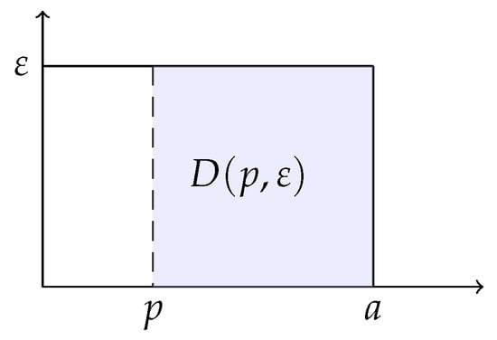
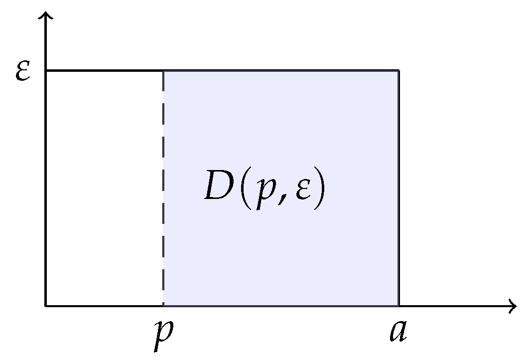
Consumers are heterogeneous in that they may have a different valuation for the product—a consumer’s valuation of the product is how much he or she is willing to pay for the product. Consumers are uniformly distributed between 0 and a according to their product evaluations. Let $\epsilon$ be the density of consumers, that is, the number of consumers for any given value of consumers. We assume $\epsilon$ is a random variable. See Figure 1 for an illustration of the distribution of consumers.

Figure 1. The distribution of consumers.

Consumers with a valuation greater than or equal to p will buy this product. So, the demand for the product is $D(p,\epsilon )=\epsilon (a-p)$. For such a multiplicative model, the uncertainty of demand can be shown as the uncertainty of the market intensity.

We further assume that the consumer density $\epsilon$ follows a Bernoulli distribution,

$$\epsilon =\left\{\begin{array}{c}1-\delta ,\mathrm{with}\mathrm{probability}{\displaystyle \frac{1}{2}},\hfill \\ 1+\delta ,\mathrm{with}\mathrm{probability}{\displaystyle \frac{1}{2}},\hfill \end{array}\right.$$

(1)

where $\delta \in [0,1]$. The Bernoulli specification is adopted for three reasons. First, it is the simplest nontrivial representation of market uncertainty that retains the essential trade-off of the newsvendor problem: a high-demand state ($ϵ=1+\delta$) and a low-demand state ($ϵ=1-\delta$) with equal probability. Similar high-or-low market demand has been used in papers. Second, it enables fully closed-form equilibrium expressions, which are essential for the comparative statics and the identification of the optimal overconfidence levels in Propositions 3 and 4. Third, although real market demand is seldom literally binary, the Bernoulli model captures the structure of demand uncertainty, the mean and the variance, which are exactly the dimensions on which overprecision operates.

Therefore, the product demand is price dependent and stochastic as follows:

$$D(p)=\left\{\begin{array}{c}(1-\delta )(a-p),\mathrm{with}\mathrm{probability}{\displaystyle \frac{1}{2}};\hfill \\ (1+\delta )(a-p),\mathrm{with}\mathrm{probability}{\displaystyle \frac{1}{2}}.\hfill \end{array}\right.$$

$s<c<w<a$ is assumed throughout the analysis. The parametric restriction is structural rather than merely convenient, and each inequality has a clear economic meaning. (i) $s<c$: The salvage value is below the manufacturer’s unit cost; otherwise the retailer could always recover the full ordering cost from salvaging, eliminating the newsvendor trade-off and making the model degenerate. (ii) $c<w$: The wholesale price exceeds the unit cost, which is the manufacturer’s participation constraint; with $w\le c$, the manufacturer would earn a non-positive profit and exit the market. (iii) $w<a$: The wholesale price is below the maximum consumer valuation, which guarantees a positive expected demand ($a-w>0$) and hence a profitable retail operation; if $w\ge a$, no consumer would buy and the market collapses. Together, these inequalities ensure that both channel members have positive equilibrium profits.

3.2. Unbiased Retailer’s Problem

The pricing and ordering decisions of an unbiased retailer based on a given wholesale price w are examined.

Note that the realized demand is either $(1-\delta )(a-p)$ or $(1+\delta )(a-p)$. So, for a fixed retail price p, the demand for the product is at least $(1-\delta )(a-p)$. The retailer can always sell at least $(1-\delta )(a-p)$ products providing that their stock is enough. Choosing an order quantity smaller than $(1-\delta )(a-p)$ means that the retailer gives up the profit by $p-w$ per unit. Therefore, the retailer chooses an order quantity of at least $(1-\delta )(a-p)$.

The demand is at most $(1+\delta )(a-p)$. If the retailer chooses an order quantity that is greater than $(1+\delta )(a-p)$, the stock exceeding $(1+\delta )(a-p)$ cannot be sold regardless of the demand. The overstock will cost the retailer $w-s$ per unit. So, the retailer chooses an order quantity of at most $q=(1+\delta )(a-p)$. In summary, the order quantity q should be in the interval $\left[(1-\delta )(a-p),(1+\delta )(a-p)\right]$.

Given the retail price p and the order quantity q, the expected profit of the retailer is

$${\pi }_r(p,q)={\displaystyle \frac{1}{2}}pq+{\displaystyle \frac{1}{2}}\left\{p(1-\delta )(a-p)+s[q-(1-\delta )(a-p)]\right\}-wq.$$

(2)

The first term above is sales when the high demand density is realized, i.e., $q=(1+\delta )(a-p)$. The second term is sales plus the salvage value from the leftover inventory when the low demand density is realized, i.e., $q=(1-\delta )(a-p)$. The third term is the ordering cost.

The retailer faces the problem of choosing a pair of $\{p,q\}$ to maximize ${\pi }_r(p,q)$.

The first-order derivative of ${\pi }_r(p,q)$ with respect to q is

$${\displaystyle \frac{\partial {\pi }_r(p,q)}{\partial q}}={\displaystyle \frac{1}{2}}p+{\displaystyle \frac{1}{2}}s-w.$$

Consequently, when $p<2w-s$, $\partial {\pi }_r(p,q)/\partial q<0$, which means that ${\pi }_r(p,q)$ is decreasing in q. The retailer should choose to order $(1-\delta )(a-p)$. Similarly, when $p\ge 2w-s$, the retailer should order $(1+\delta )(a-p)$. In summary, the optimal order quantity given retail price p is

$$q^{*}(p)=\left\{\begin{array}{c}(1-\delta )(a-p),p<2w-s;\hfill \\ (1+\delta )(a-p),\mathrm{otherwise}.\hfill \end{array}\right.$$

(3)

Substituting (3) into (2), the retailer’s best profit function given price p is obtained:

$${\pi }_r(p)=\left\{\begin{array}{cc}(1-\delta )(a-p)(p-w),\hfill & p<2w-s;\hfill \\ (a-p)[p-w-\delta (w-s)],\hfill & \mathrm{otherwise}.\hfill \end{array}\right.$$

Next, we characterize the optimal price of the retailer. For ease of exposition, we denote

$$w_0={\displaystyle \frac{2-\sqrt{1-\delta }}{3+\delta }}a+\left(1-{\displaystyle \frac{2-\sqrt{1-\delta }}{3+\delta }}\right)s,$$

(4)

which is a weighted sum of a and s. The weight of a, ${\displaystyle \frac{2-\sqrt{1-\delta }}{3+\delta }}$, is increasing from ${\displaystyle \frac{1}{3}}$ at $\delta =0$ to ${\displaystyle \frac{1}{2}}$ at $\delta =1$.

Lemma 1.

Given a wholesale price w, the optimal retail price for the retailer is

$$p^{*}(w)=\left\{\begin{array}{cc}{p}_H={\displaystyle \frac{1}{2}}[a+(1+\delta )w-\delta s],\hfill & w\le w_0;\hfill \\ p_L={\displaystyle \frac{1}{2}}(a+w),\hfill & w>w_0.\hfill \end{array}\right.$$

The proofs of lemmas and propositions are given in Appendix A.

From Lemma 1, the retailer chooses between two prices, $p_H$ or $p_L$, according to the wholesale prices. The manufacturer can influence the retailer’s behavior through the wholesale price.

Applying Lemma 1 to Equation (3), the retailer’s best order quantity is obtained. When $w>w_0$, $p^{*}=p_L$ and so $q^{*}(p_L)=(1-\delta )(a-p_L)={\displaystyle \frac{1}{2}}(1-\delta )(a-w):=q_L$; when $w\le w_0$, $p^{*}=p_H$ and so $q^{*}(p_H)=(1+\delta )(a-p_H)={\displaystyle \frac{1}{2}}(1+\delta )[a-w-\delta (w-s)]:=q_H$. Obviously, $q_H>q_L$. Hence, given the wholesale price w, the retailer’s optimal order quantity is as follows.

$$q^{*}(w)=\left\{\begin{array}{cc}{q}_H={\displaystyle \frac{1}{2}}(1+\delta )[a-(1+\delta )w+\delta s],\hfill & w\le w_0;\hfill \\ q_L={\displaystyle \frac{1}{2}}(1-\delta )(a-w),\hfill & w>w_0.\hfill \end{array}\right.$$

(5)

Moreover, given the wholesale price w, the optimal profit of the retailer is

$${\pi }_r^{*}(w)=\left\{\begin{array}{cc}{\displaystyle \frac{1}{4}}{[a+\delta s-(1+\delta )w]}^2,\hfill & w\le w_0;\hfill \\ {\displaystyle \frac{1}{4}}(1-\delta ){(a-w)}^2,\hfill & w>w_0.\hfill \end{array}\right.$$

(6)

In general, given the manufacturer’s wholesale price w, the retailer’s optimal order quantity and profit are given in (5) and (6), respectively. When $w\le w_0$, the order quantity equals the maximum demand $(1+\delta )(a-p_H)$ and so the inventory can always satisfy the demand. We refer to this situation as the overstocking order. When $w>w_0$, the order quantity equals the minimum demand $(1-\delta )(a-p_L)$ and so there will never be leftover inventory. We refer to this situation as the understocking order. Hence, with regard to different wholesale prices, the retailer will choose either an overstocking or an understocking order. When $w=w_0$, the retailer makes the same profit with two different pricing and ordering strategies, in which case ordering more is naturally better. So, we assume that the retailer will choose the price $p_H$ and $q_H$ when $w^{*}=w_0$.

3.3. Manufacturer’s Problem

In this section, we examine the manufacturer’s pricing decision.

The profit function of the manufacturer is

$${\pi }_m(w)=(w-c)q^{*}(w)=\left\{\begin{array}{cc}{\displaystyle \frac{1}{2}}(1+\delta )(w-c)\left[a-w-\delta (w-s)\right],\hfill & w\le w_0;\hfill \\ {\displaystyle \frac{1}{2}}(1-\delta )(w-c)(a-w),\hfill & w>w_0.\hfill \end{array}\right.$$

(7)

First, we show the following lemma, where

$$\begin{array}{cc}\hfill f_1(\delta )=& {\displaystyle \frac{4-2\sqrt{1-\delta }}{3+\delta }}-{\displaystyle \frac{1}{1+\delta }},\hfill \\ \hfill f_2(\delta )=& {\displaystyle \frac{2\sqrt{1-\delta }-1+\delta \left[2+4\sqrt{1-\delta }+\delta (2\sqrt{1-\delta }-1)\right]-2\sqrt{\delta (1+\sqrt{1-\delta }+\delta )(1-{\delta }^2)(3+\delta )}}{(\delta -1)(3+\delta )}}.\hfill \end{array}$$

(8)

Lemma 2.

For $\delta \in (0,1)$, $f_1(\delta )<f_2(\delta )$.

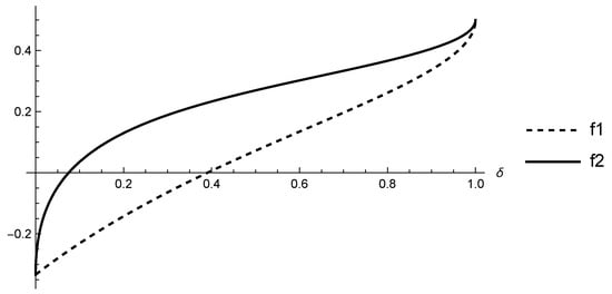
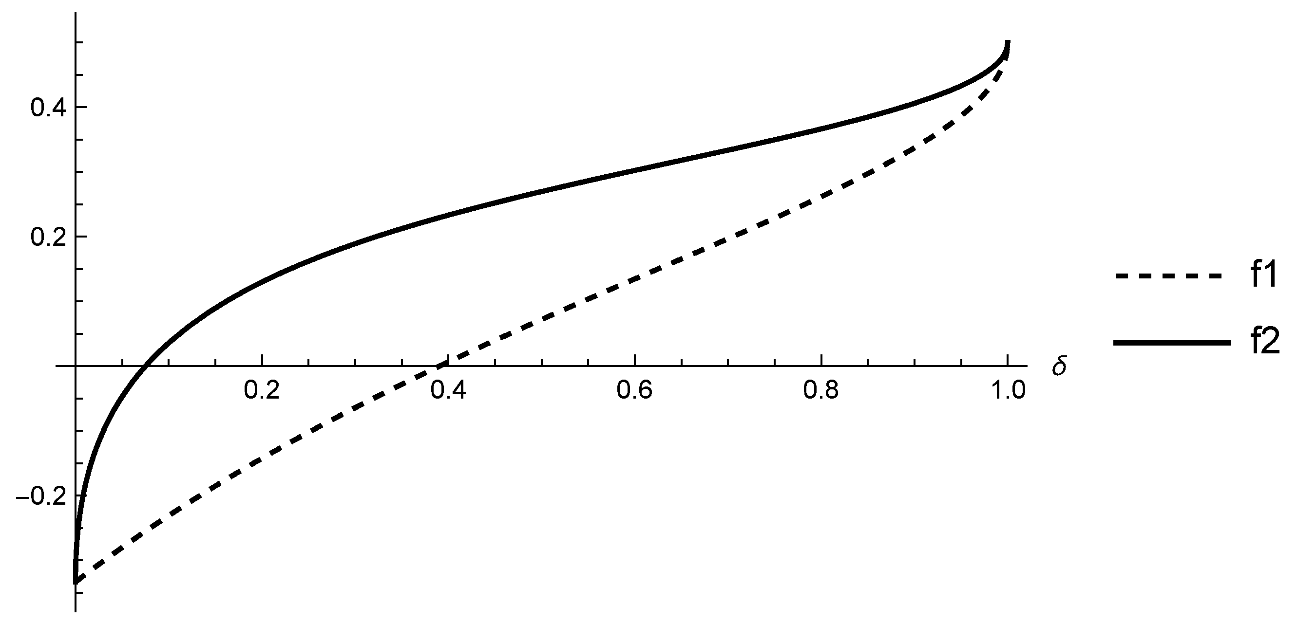
We illustrate $f_1(\delta )$ and $f_2(\delta )$ in Figure 2, where we can see that both $f_1(\delta )$ and $f_2(\delta )$ are increasing and $f_1(\delta )<f_2(\delta )$.

Figure 2. $f_1(\delta )$ and $f_2(\delta )$.

We further let

$$\begin{array}{c}\hfill c_1=[1-f_1(\delta )]s+f_1(\delta )a,\\ \hfill c_2=[1-f_2(\delta )]s+f_2(\delta )a.\end{array}$$

(9)

Surely, $c_2>c_1$. $c_1$ is the first (lower) cost threshold of the unbiased model. $c_2$ is the second (upper) cost threshold of the unbiased model. Now we characterize the optimal wholesale price for the manufacturer in the following lemma.

Lemma 3.

The manufacturer’s optimal wholesale price is

$$\begin{array}{c}\hfill w^{*}=\left\{\begin{array}{cc}{\displaystyle \frac{1}{2}}(c+{\displaystyle \frac{a+\delta s}{1+\delta }}),\hfill & c\le c_1;\hfill \\ w_0={\displaystyle \frac{2-\sqrt{1-\delta }}{3+\delta }}a+(1-{\displaystyle \frac{2-\sqrt{1-\delta }}{3+\delta }})s,\hfill & c_1<c\le c_2;\hfill \\ {\displaystyle \frac{1}{2}}(c+a),\hfill & c>c_2.\hfill \end{array}\right.\end{array}$$

(10)

Substituting $w^{*}$ into Lemma 1, Equations (5)–(7), we obtain the equilibrium results given in Equations (11)–(13). Taking the retailer’s decision into consideration, we get the optimal pricing decision of the retailer. The optimal decisions for both the manufacturer and the retailer depend on which interval the manufacturer’s product cost belongs to.

Formally, the retailer’s optimal ordering policy is characterized by two extreme quantities: $q_H=(1+\delta )(a-p_H)$ (the overstocking order, which can always satisfy demand but may leave unsold inventory) and $q_L=(1-\delta )(a-p_L)$ (the understocking order, which never leaves leftover inventory but forgoes potential sales in high-demand states). The intermediate regime $c_1<c\le c_2$ corresponds to a third configuration in which the manufacturer’s optimal wholesale price $w_0$ keeps the retailer exactly indifferent between these two orders (Lemma 1); we refer to it as the intermediate (threshold) regime.

Why do the three situations occur as the production cost varies?

(1) Low cost ($c\le c_1$): With a large margin, the manufacturer can afford to concede price for volume—charging a low wholesale price to induce the retailer to stock heavily, earning through quantity. Part of the demand risk is borne by the manufacturer (implicitly, through the low wholesale price). (2) High cost ($c>c_2$): The margin is thin and the concession is no longer affordable; the manufacturer switches to price extraction—raising the wholesale price to $(a+c)/2$, so the retailer orders only the minimum demand and the stockout risk in high-demand states is shifted entirely onto the retailer. (3) Intermediate cost ($c_1<c\le c_2$): The manufacturer is at a critical balance—the two strategies (low price for volume vs. high price for margin) yield comparable profits, and the optimum falls exactly at $w_0$, the price that leaves the retailer indifferent.

The three regimes emerge because the retailer’s binary ordering response, combined with the manufacturer’s two-segment profit function, is successively pushed across the two thresholds $c_1$ and $c_2$ as the production cost c varies around the switching point $w_0$. At bottom, the pattern reflects how the allocation of inventory risk between the upstream and downstream channel members flips with the cost.

The equilibrium outcomes of the unbiased retailer and the manufacturer are as follows:

(1)

$c\le c_1$,

$$\begin{array}{cc}\hfill w^{*}& ={\displaystyle \frac{1}{2}}(c+{\displaystyle \frac{a+\delta s}{1+\delta }}),\hfill \\ \hfill p^{*}& ={\displaystyle \frac{1}{4}}(3a+c+\delta c-\delta s),\hfill \\ \hfill q^{*}& ={\displaystyle \frac{1}{4}}(1+\delta )(a+\delta s-\delta c-c),\hfill \\ \hfill {\pi }_m^{*}& ={\displaystyle \frac{1}{8}}{[a-(1+\delta )c+\delta s]}^2,\hfill \\ \hfill {\pi }_r^{*}& ={\displaystyle \frac{1}{16}}{[a-(1+\delta )c+\delta s]}^2.\hfill \end{array}$$

(11)

(2)

$c_1<c\le c_2$,

$$\begin{array}{cc}\hfill w^{*}& ={\displaystyle \frac{2-\sqrt{1-\delta }}{3+\delta }}a+(1-{\displaystyle \frac{2-\sqrt{1-\delta }}{3+\delta }})s,\hfill \\ \hfill p^{*}& ={\displaystyle \frac{(3+\sqrt{1-\delta }+\delta )a+(1+\sqrt{1-\delta }-\delta )s}{2(2+\sqrt{1-\delta })}},\hfill \\ \hfill q^{*}& ={\displaystyle \frac{(1+\sqrt{1-\delta }-\delta )(1+\delta )(a-s)}{2(2+\sqrt{1-\delta })}},\hfill \\ \hfill {\pi }_m^{*}& ={\displaystyle \frac{(1+\sqrt{1-\delta }-\delta )(1+\delta )(a-s)[a-(2+\sqrt{1-\delta })c+s+\sqrt{1-\delta }s]}{2{(2+\sqrt{1-\delta })}^2}},\hfill \\ \hfill {\pi }_r^{*}& ={\displaystyle \frac{{(1+\sqrt{1-\delta }-\delta )}^2{(a-s)}^2}{4{(2+\sqrt{1-\delta })}^2}}.\hfill \end{array}$$

(12)

(3)

$c>c_2$,

$$\begin{array}{cc}\hfill w^{*}& ={\displaystyle \frac{1}{2}}(a+c),\hfill \\ \hfill p^{*}& ={\displaystyle \frac{1}{4}}(3a+c),\hfill \\ \hfill q^{*}& ={\displaystyle \frac{1}{4}}(1-\delta )(a-c),\hfill \\ \hfill {\pi }_m^{*}& ={\displaystyle \frac{1}{8}}(1-\delta ){(a-c)}^2,\hfill \\ \hfill {\pi }_r^{*}& ={\displaystyle \frac{1}{16}}(1-\delta ){(a-c)}^2.\hfill \end{array}$$

(13)

The manufacturer has three choices for the wholesale price depending on the interval to which the production cost belongs. Keeping Lemma 1 in mind, comparing $w^{*}$ with $w_0$, we know that $c\le c_1$ corresponds to the overstocking case and $c>c_2$ corresponds to the understocking case. When $c_1<c\le c_2$, $w^{*}=w_0$, the retailer is indifferent between two ordering quantities. And the retailer chooses the overstocking order policy because ordering more does not hurt. If the wholesale price is slightly higher, the retailer will choose the understocking order and vice versa.

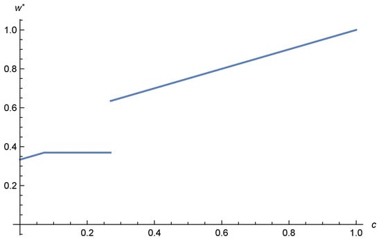
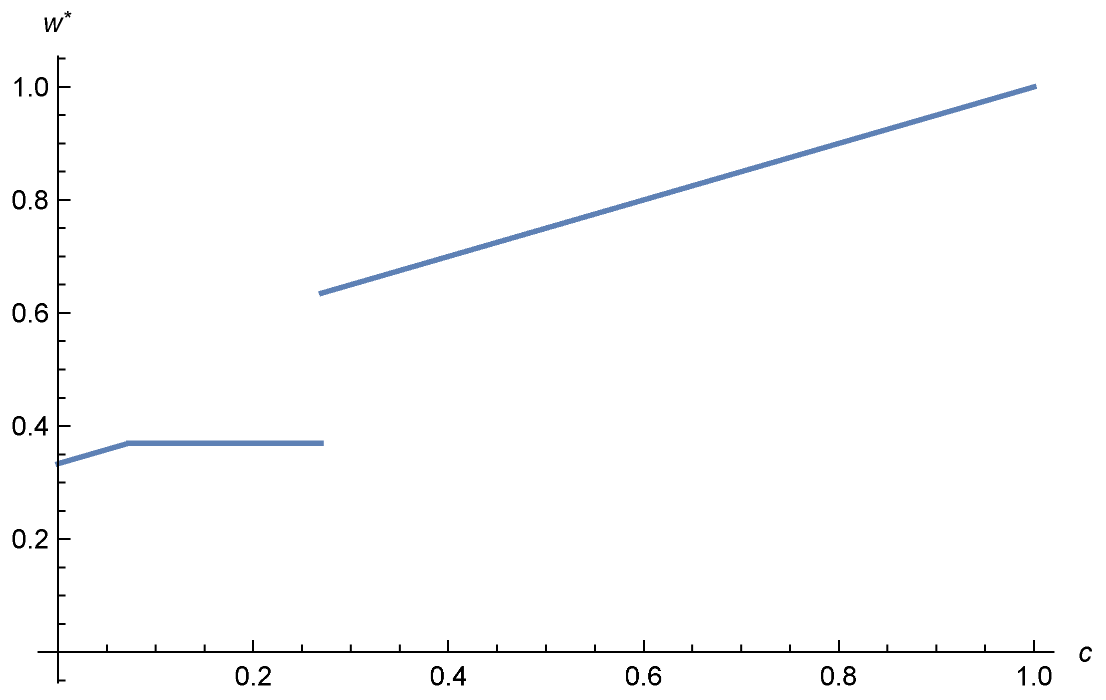
It is obvious that the optimal wholesale price in the overstocking case $w^{*}={\displaystyle \frac{1}{2}}(a+c-{\displaystyle \frac{\delta (a-s)}{1+\delta }})$ is lower than that in the understocking case $w^{*}={\displaystyle \frac{1}{2}}(a+c)$. It is easy to see that $w^{*}$ increases in $c\le c_1$ and $c>c_2$, but is a constant in $c\in (c_1,c_2]$. Then, a natural question is whether $w^{*}$ is increasing at $c=c_1$ and $c=c_2$. Numerically, the change in $w^{*}$ with c is shown in Figure 3 with $a=1$, $s=0$, and $\delta =0.5$. The wholesale price jumps at $c=c_2$.

Figure 3. The optimal wholesale price when $a=1,s=0$, and $\delta =0.5$.

The following proposition gives some properties of the optimal $w^{*}$, $p^{*}$, and $q^{*}$.

Proposition 1.

(1) The wholesale price $w^{*}$ decreases in δ for $c\le c_1$, increases in δ for $c\in (c_1,c_2]$, and is independent of δ for $c>c_2$.

(2) The retail price $p^{*}$ increases in δ for $c\le c_2$ and is independent of δ for $c>c_2$.

(3) The order quantity $q^{*}$ is concave in δ for $c\le c_2$ and decreases in δ for $c>c_2$.

In the overstocking case ($c\le c_1$), the optimal wholesale price $w^{*}={\displaystyle \frac{1}{2}}(c+{\displaystyle \frac{a+\delta s}{1+\delta }})$ consists of two parts: one related to the production cost and the other a mark-up that decreases with demand volatility. In this case, the manufacturer shares the risk of demand uncertainty. When demand volatility is high, the risk to the retailer is large, and the manufacturer shares the risk by decreasing the wholesale price. The reason $p^{*}$ increases in $\delta$ is that higher volatility means more risk for the retailer and that a higher retail price helps the retailer withstand the risk.

In the intermediate case ($c_1<c\le c_2$), both $w^{*}$ and $p^{*}$ are increasing in $\delta$. In this situation, the wholesale price is determined by the market scale a and the salvage value s with weights depending on the demand volatility $\delta$. That $w^{*}=w_0$ is the wholesale price that makes the retailer indifferent between the two ordering quantities (see the proof of Lemma 1). The higher the volatility, the larger the difference between the profits obtained by the retailer with the overstocking or understocking order will be. Since increasing the wholesale price will narrow the difference, $w^{*}$ is increasing in $\delta$. Thus, the greater the volatility, the higher the wholesale price will be. The optimal price $p^{*}$ changes for the same reason as in the overstocking case, that is, higher volatility implies greater risk to the retailer, and a higher retail price helps the retailer to withstand the risk.

In the understocking case ($c>c_2$), the wholesale and retail prices do not respond to the volatility level, but the order quantity is decreasing in $\delta$. This is because the order quantity is the minimum demand of the product, and the minimum demand is decreasing in $\delta$.

4. The Supply Chain with an Overconfident Retailer

In this section, we study the supply chain with an overconfident retailer. We want to see how the overconfident retailer influences the decisions and profits of the retailer itself, the manufacturer, and the supply chain.

4.1. Overconfident Retailer’s Profit

Compared with an unbiased retailer, an overconfident retailer perceives market uncertainty as ${\epsilon }_{oc}:=\alpha \mu +(1-\alpha )\epsilon$ for some $\alpha \in [0,1]$, with $\mu =E(\epsilon )=1$. The real market uncertainty is given in Equation (1). The value of parameter $\alpha$ measures the level of overconfidence of the retailer: the greater the value of $\alpha$ is, the greater the overconfidence of the retailer will be. In the extreme case, $\alpha =0$ means that the retailer is unbiased and $\alpha =1$ means that the retailer thinks of the demand as constant. This setting is used in many papers, e.g., [13].

From Equation (1),

$${\epsilon }_{oc}=\left\{\begin{array}{c}1-(1-\alpha )\delta ,\mathrm{with}\mathrm{probability}{\displaystyle \frac{1}{2}};\hfill \\ 1+(1-\alpha )\delta ,\mathrm{with}\mathrm{probability}{\displaystyle \frac{1}{2}}.\hfill \end{array}\right.$$

Therefore, the demand perceived by the overconfident retailer is $D_{oc}(p)={\epsilon }_{oc}(a-p)$. Hence, an overconfident retailer perceives demand volatility as being reduced from $\delta$ to $(1-\alpha )\delta$. So, the higher the overconfidence, the more the demand volatility will be reduced.

Although the overconfident retailer perceives the demand differently from an unbiased retailer, the retailer does not realize this. Thus, the overconfident retailer behaves following the same logic as the unbiased retailer and their decisions on price and the order quantity are the same as those of an unbiased retailer with demand as $D_{oc}(p)$. This treatment follows the canonical overprecision modeling in Ren and Croson (2013) [11] and Li (2019) [13]; in particular, the overprecision parameter $\alpha$ is treated as a stable trait of the decision-maker, not as a state variable updated through Bayesian learning. We acknowledge that this is a simplification: in a multi-period setting with realized-demand feedback, a Bayesian retailer would update their posterior distribution, gradually shrinking the gap between perceived and true variance. Such dynamic learning is outside the scope of the present single-period model and is identified as a promising future research direction in Section 5.2.

Hence, all the results obtained in the last section become those for the setting with the overconfident retailer, except that $\delta$ is replaced by ${\delta }^{\prime }=(1-\alpha )\delta$. For example, the overconfident retailer perceives the demand as

$$D_{oc}(p)=\left\{\begin{array}{c}(1-{\delta }^{\prime })(a-p),\mathrm{with}\mathrm{probability}{\displaystyle \frac{1}{2}};\hfill \\ (1+{\delta }^{\prime })(a-p),\mathrm{with}\mathrm{probability}{\displaystyle \frac{1}{2}}.\hfill \end{array}\right.$$

Similarly to Lemma 1 in Section 3.2, the overconfident retailer’s pricing strategy given the wholesale price w is

$$p_{oc}^{*}(w)=\left\{\begin{array}{cc}{p}_{ocH}={\displaystyle \frac{1}{2}}[a+(1+{\delta }^{\prime })w-{\delta }^{\prime }s],\hfill & w\le w_m,\hfill \\ p_{ocL}={\displaystyle \frac{1}{2}}(a+w),\hfill & w>w_m,\hfill \end{array}\right.$$

where $w_m$ is exactly $w_0$ in (4) with ${\delta }^{\prime }$, i.e.,

$$w_m={\displaystyle \frac{2-\sqrt{1-{\delta }^{\prime }}}{3+{\delta }^{\prime }}}a+\left(1-{\displaystyle \frac{2-\sqrt{1-{\delta }^{\prime }}}{3+{\delta }^{\prime }}}\right)s.$$

(14)

From Equation (5), the order quantity given wholesale price w is

$$q_{oc}^{*}(w)=\left\{\begin{array}{cc}{q}_{ocH}={\displaystyle \frac{1}{2}}(1+{\delta }^{\prime })[a-(1+{\delta }^{\prime })w+{\delta }^{\prime }s],\hfill & w\le w_m;\hfill \\ q_{ocL}={\displaystyle \frac{1}{2}}(1-{\delta }^{\prime })(a-w),\hfill & w>w_m.\hfill \end{array}\right.$$

(15)

Based on $q_{oc}^{*}(w)$, the manufacturer’s profit is still ${\pi }_m(w)=(w-c)q_{oc}^{*}(w)$, similar to (7). So, the manufacturer’s optimal wholesale price is exactly $w^{*}$ given in (4) with ${\delta }^{\prime }$, i.e.,

$$\begin{array}{c}\hfill w_{oc}^{*}=\left\{\begin{array}{cc}{\displaystyle \frac{1}{2}}(c+{\displaystyle \frac{a+(1-\alpha )\delta s}{1+(1-\alpha )\delta }}),\hfill & c\le c_l;\hfill \\ {\displaystyle \frac{2-\sqrt{1-(1-\alpha )\delta }}{3+(1-\alpha )\delta }}a+(1-{\displaystyle \frac{2-\sqrt{1-(1-\alpha )\delta }}{3+(1-\alpha )\delta }})s,\hfill & c_l<c\le c_h;\hfill \\ {\displaystyle \frac{1}{2}}(a+c),\hfill & c>c_h.\hfill \end{array}\right.\end{array}$$

(16)

where $c_h$ and $c_l$ are, respectively, $c_2$ and $c_1$ in (10) with ${\delta }^{\prime }$, i.e.,

$$c_l=f_1({\delta }^{\prime })a+[1-f_1({\delta }^{\prime })]s,c_h=f_2({\delta }^{\prime })a+[1-f_2({\delta }^{\prime })]s.$$

(17)

$c_l$ is the lower cost threshold in the overconfident model. $c_h$ is the upper cost threshold in the overconfident model.

Let $p_{oc}^{*}=p_{oc}(w_{oc}^{*})$, $q_{oc}^{*}=q_{oc}(w_{oc}^{*})$, and ${\pi }_{moc}^{*}=(w_{oc}^{*}-c)q_{oc}^{*}$. Hence, $w_{oc}^{*}$, $p_{oc}^{*}$, $q_{oc}^{*}$, and ${\pi }_{moc}^{*}$ are the same as those given in Equations (11)–(13), except that $\delta$ is replaced by ${\delta }^{\prime }$.

When $c\le c_l$, similar to the unbiased retailer, the manufacturer’s optimal wholesale price makes the retailer choose the overstocking order quantity $(1+{\delta }^{\prime })(a-p_{oc}^{*})$. When $c>c_h$, the optimal wholesale price makes the retailer choose the understocking order quantity $(1-{\delta }^{\prime })(a-p_{oc}^{*})$. When $c_l<c\le c_h$, the retailer chooses the intermediate order quantity $(1+{\delta }^{\prime })(a-p_{oc}^{*})$.

In the following proposition, we study the sensitivity of $w_{oc}^{*}$, $p_{oc}^{*}$, and $q_{oc}^{*}$ to the parameter $\alpha$, which are rewritten as functions of $\alpha$: $w_{oc}^{*}(\alpha )$, $p_{oc}^{*}(\alpha )$, and $q_{oc}^{*}(\alpha )$, respectively.

Proposition 2.

(1) The wholesale price $w_{oc}^{*}(\alpha )$ is increasing in α for $c\le c_l$, decreasing in α for $c\in [c_l,c_h)$, and is independent of α for $c>c_h$.

(2) The retail price $p_{oc}^{*}(\alpha )$ is decreasing in α for $c\le c_h$ and is independent of α for $c>c_h$.

(3) The order quantity $q_{oc}^{*}(\alpha )$ is concave for $c\le c_h$ and increases in α for $c>c_h$.

The above proposition immediately follows from Proposition 1 by noting that $w_{oc}^{*}$, $p_{oc}^{*}$, and $q_{oc}^{*}$ are exactly $w^{*}$, $p^{*}$, and $q^{*}$ given in Equations (11)–(13) with $\delta$ replaced by ${\delta }^{\prime }=(1-\alpha )\delta$.

Both $p_{oc}^{*}(w)$ and $q_{oc}^{*}(w)$ are determined by the retailer who believes the uncertainty level is ${\delta }^{\prime }$. However, the overconfident retailer’s realized profit is different, because the uncertainty level in the realized demand is still $\delta$, instead of ${\delta }^{\prime }$. Let ${\pi }_{roc}(p,q|w)$ denote the overconfident retailer’s realized profit when the price is p and the order quantity is q, given the wholesale price w. Then, similar to (2),

$${\pi }_{roc}(p,q|w)={\displaystyle \frac{1}{2}}\{p(1-\delta )(a-p)+s[q-(1-\delta )(a-p)]\}+{\displaystyle \frac{1}{2}}pq-qw.$$

(18)

Let ${\pi }_{roc}^{*}(\alpha )={\pi }_{roc}(p_{oc}^{*},q_{oc}^{*}|w_{oc}^{*})$ be the retailer’s optimal profit. After some algebraic computations, we can obtain the expression of ${\pi }_{roc}^{*}$.

$${\pi }_{roc}^{*}=\left\{\begin{array}{cc}-{\displaystyle \frac{1}{32}}\{a-c[1+(1-\alpha )\delta ]+\delta s(1-\alpha )\}\hfill & \hfill \\ \left\{c\right[1+(1-\alpha )\delta ](2+\delta \alpha )-a(2-3\delta \alpha )-\delta s[2+(2+\delta -\alpha \delta )\alpha \left]\right\},\hfill & c\le c_l\hfill \\ -{\displaystyle \frac{{(a-s)}^2\{-2[\sqrt{(\alpha -1)\delta +1}+1]+({\alpha }^2-1){\delta }^2+\delta [2\sqrt{(\alpha -1)\delta +1}-\alpha +3]\}}{4{(\sqrt{(\alpha -1)\delta +1}+2)}^2}},\hfill & c_l<c\le c_h\hfill \\ -{\displaystyle \frac{1}{32}}(a-c)\{c(2-2\delta +3\delta \alpha )-4\delta s\alpha -a[2-\delta (2+\alpha )]\},\hfill & c>c_h\hfill \end{array}\right.$$

(19)

In the following proposition, we characterize the change in the retailer’s profit with the level of overconfidence $\alpha$.

Proposition 3.

The retailer’s profit ${\pi }_{roc}^{*}(\alpha )$ decreases with α, except that, for $c_l<c\le c_h$, ${\pi }_{roc}^{*}(\alpha )$ increases with $\alpha \le {\alpha }_1(\delta )$ for some ${\alpha }_1(\delta )\in (0,1)$; in particular, ${\alpha }_1(\delta )=1$ when $\delta \le {\displaystyle \frac{2}{5}}$.

${\alpha }_1(\delta )$ is the retailer’s profit-maximizing (optimal) overconfidence level.

In the overstocking case, by Proposition 2, overconfidence causes the retailer to set a lower retail price and the manufacturer to charge a higher wholesale price. The profit margin decreases. Overconfidence makes the retailer worse off.

In the intermediate case, also from Proposition 2, overconfidence makes the retailer set a lower retail price and, further, the manufacturer charges a lower wholesale price. This gives the retailer an opportunity to benefit. Proposition 3 shows that overconfidence will make the retailer better off when the level of overconfidence is not too large, but worse off otherwise.

In the understocking case, the overconfident retailer orders too many products, while the wholesale price and the retail price are independent of $\alpha$. Hence, the mismatch between inventory and demand makes the retailer worse off.

Intuitively, the overconfidence will hurt the retailer, since they cannot judge the market uncertainty and deviate from optimal decisions. However, the above propositions show that the retailer’s overconfidence can either hurt or benefit the retailer itself according to the level of overconfidence and the manufacturer’s production cost. In detail, the retailer’s overconfidence hurts the retailer itself, except when the production cost is medium and the level of overconfidence is not too large, the retailer’s overconfidence benefits itself.

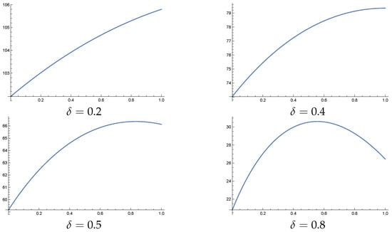
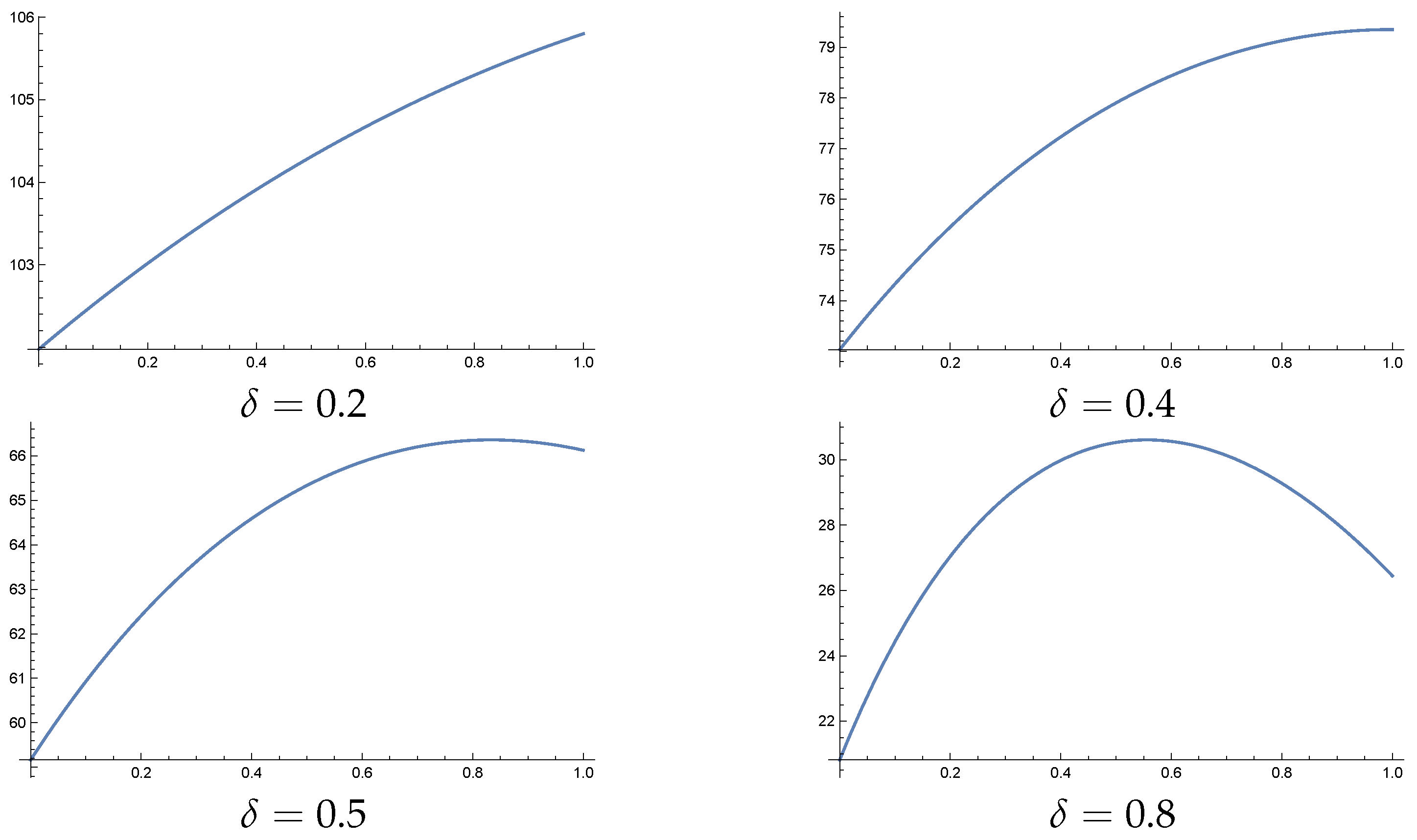
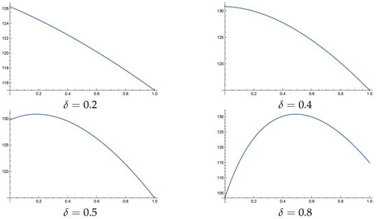
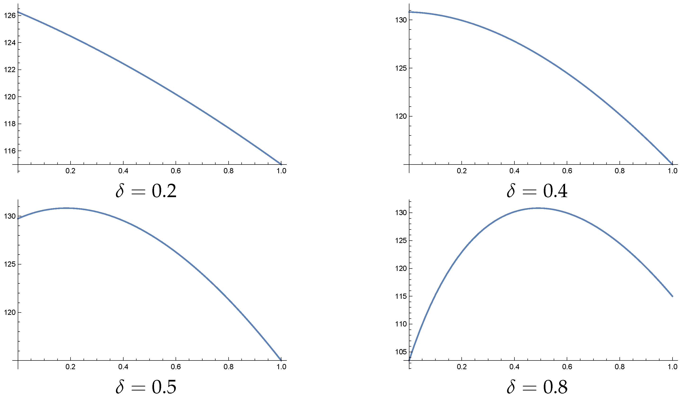
Figure 4 gives a numerical analysis (with $a=35$, $c=2$ and $s=0.5$) for the change in the retailer’s profit with $\alpha$ at different values of $\delta$ when $c_l<c\le c_h$. The results are consistent with those given in Proposition 3. We find that when $\delta <{\displaystyle \frac{2}{5}}$, the retailer’s profit always increases with the level of overconfidence, i.e., the optimal level of overconfidence for the retailer is ${\alpha }_1(\delta )=1$. When $\delta >{\displaystyle \frac{2}{5}}$, ${\alpha }_1(\delta )<1$ and the retailer’s profit first increases with $\alpha$ and then decreases with $\alpha$. We further find that the optimal level of overconfidence ${\alpha }_1(\delta )$ is decreasing in $\delta$. That is, with the increase of $\delta$ the maximum point of the retailer’s profit (i.e., the optimal level of overconfidence) shifts from right to left. This is also to say that when market volatility increases, the retailer’s optimal level of overconfidence decreases.

Figure 4. Changes in the retailer’s profit with $\alpha$ for different values of $\delta$ when $c_l<c\le c_h$.

4.2. The Manufacturer’s Profit

The manufacturer’s profit ${\pi }_{moc}^{*}=(w_{oc}^{*}-c)q_{oc}^{*}$, written as a function of $\alpha$, is as follows:

$${\pi }_{moc}^{*}=\left\{\begin{array}{cc}{\displaystyle \frac{1}{8}}{\{a-[1+(1-\alpha )\delta ]c+\delta s\}}^2,\hfill & c\le c_l\hfill \\ {\displaystyle \frac{[1+\sqrt{1-(1-\alpha )\delta }-(1-\alpha )\delta ][1+(1-\alpha )\delta ](a-s)[a-(2+\sqrt{1-(1-\alpha )\delta })c+s+\sqrt{1-(1-\alpha )\delta }s]}{2{(2+\sqrt{1-(1-\alpha )\delta })}^2}},\hfill & c_l<c\le c_h\hfill \\ {\displaystyle \frac{1}{8}}[1-(1-\alpha )\delta ]{(a-c)}^2,\hfill & c>c_h\hfill \end{array}\right.$$

(20)

In the following proposition, we characterize the change in the manufacturer’s profit with the retailer’s level of overconfidence $\alpha$.

Proposition 4.

The manufacturer’s profit function ${\pi }_{moc}^{*}(\alpha )$ is increasing in α for $c\le c_l$ and $c>c_h$. For $c_l<c\le c_h$, ${\pi }_{moc}^{*}(\alpha )$ increases with $\alpha \le {\alpha }_2(\delta )$ but decreases with $\alpha \ge {\alpha }_2(\delta )$. Here, ${\alpha }_2(\delta )\in [0,1]$ with ${\alpha }_2(\delta )=0$ when $\delta \le {\delta }_0$ for some ${\delta }_0\in [0,1]$.

${\alpha }_2(\delta )$ is the manufacturer’s profit-maximizing (optimal) level of overconfidence.

Note that in (15) we give the response of the retailer’s order quantity to wholesale price. Then,

$$\begin{array}{c}\hfill {\displaystyle \frac{\partial q_{ocH}}{\partial w}}=-{\displaystyle \frac{1}{2}}{[1+(1-\alpha )\delta ]}^2,w\le w_m;\\ \hfill {\displaystyle \frac{\partial q_{ocL}}{\partial w}}=-{\displaystyle \frac{1}{2}}[1-(1-\alpha )\delta ],w>w_m.\end{array}$$

(21)

When $w\le w_m$, as the wholesale price increases, overconfidence mitigates the decrease in order quantity. When $w>w_m$, as the wholesale price increases, overconfidence intensifies the decrease of the order quantity.

From Proposition 2, in the overstocking case, with the increase of the level of overconfidence of the retailer $\alpha$, the manufacturer’s wholesale price increases, while from Equation (21) the retailer’s order quantity also increases. So, the manufacturer is better off from increasing $\alpha$. Similarly, in the understocking case, the wholesale price is irrelevant to the retailer’s level of overconfidence, but the retailer will order more, and so the manufacturer will benefit.

In the intermediate case, also from Proposition 2, though the wholesale price is decreasing in $\alpha$, the overconfidence may increase the order quantity. From (21), the higher the value of $\alpha$, the smaller the rate of increase in the order quantity relative to w is. Thus, when $\alpha$ is low, the increase of the order quantity outweighs the decrease in the wholesale price. So, the manufacturer’s profit increases with $\alpha$. When the retailer is too overconfident, they presume the volatility to be too small and the change in order quantity induced by the change in the wholesale price is small, so the manufacturer may be worse off. The decrease of the wholesale price plays an important role in the increase of the order quantity. That is because when the retailer is too overconfident, they become insensitive to the change in the wholesale price.

In general, when the manufacturer’s production cost is low (i.e., $c\le c_l$) or high (i.e., $c>c_h$), an overconfident retailer benefits the manufacturer. Hence, when choosing a retailer, the manufacturer should choose one who is more likely to be overconfident. However, when $c\in (c_l,c_h]$ there are some complex but interesting things, as numerically illustrated in Figure 5 with $a=35,s=0.5$ and $c=2$ for different values of $\delta$. We find from the figures that ${\delta }_0\approx 0.45$ and the manufacturer’s profit decreases with $\alpha$ when $\delta \le {\delta }_0$ but first increases with $\alpha \le {\alpha }_2(\delta )$ and then decreases with $\alpha \ge {\alpha }_2(\delta )$ when $\delta >{\delta }_0$. Furthermore, we find from the numerical results that ${\alpha }_2(\delta )$ increases with $\delta$, which is the reverse of that of the optimal confidence level for the retailer ${\alpha }_1(\delta )$. We take many other values for a, s, and c, and find that these patterns remain robust.

Figure 5. Changes in the manufacturer’s profit with $\alpha$ for different values of $\delta$ when $c_l<c\le c_h$.

It is interesting to compare the monotonicity of the profits of the manufacturer and the retailer given in Propositions 2 and 3 as follows. The manufacturer’s profit increases with $\alpha$ while the retailer’s profit decreases with $\alpha$, which is intuitive. Interestingly, however, when $c_l<c\le c_h$ and $\delta \in [{\displaystyle \frac{2}{5}}\bigvee {\delta }_0,1]$, the profits of both the manufacturer and the retailer increase with $\alpha \le {\alpha }_2(\delta )\wedge {\alpha }_1(\delta )$ but decrease with $\alpha \ge {\alpha }_2(\delta )\vee {\alpha }_1(\delta )$. In these two intervals of $\alpha$, the overconfidence of the retailer increases or decreases both the retailer’s and the manufacturer’s profits.

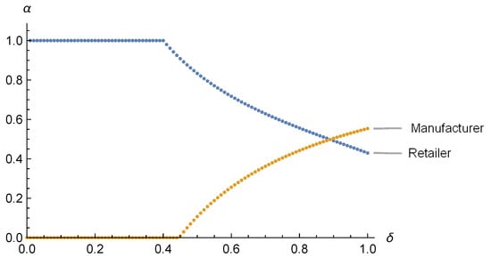
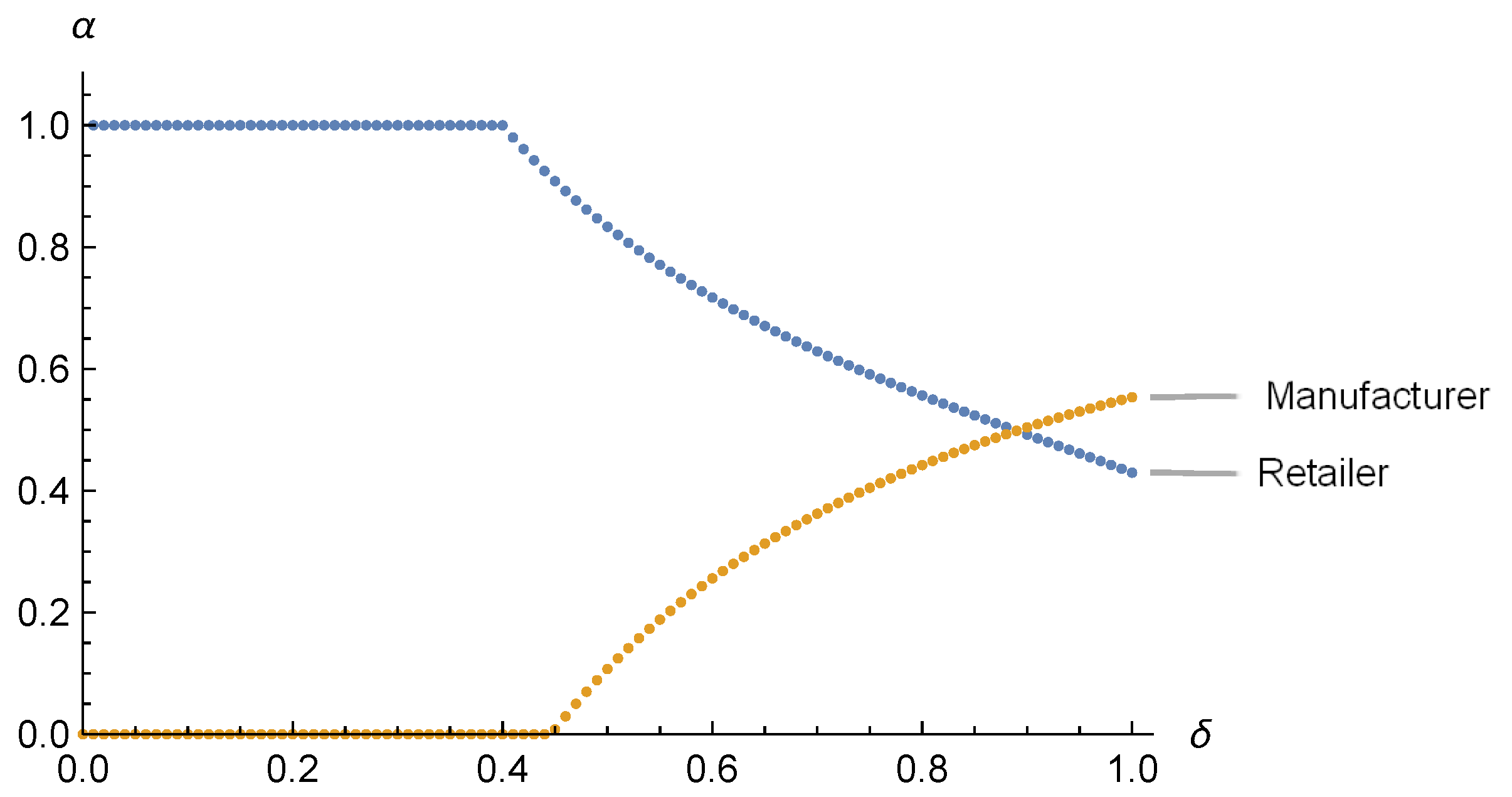
Furthermore, in Figure 6 we compare the optimal confidence levels ${\alpha }_1(\delta )$ for the retailer and ${\alpha }_2(\delta )$ for the manufacturer in regard to $\delta$ in the intermediate case. It is shown that ${\alpha }_1(\delta )=1$ for $\delta \le {\displaystyle \frac{2}{5}}$ and then decreases from ${\alpha }_1({\displaystyle \frac{2}{5}})=1$ to ${\alpha }_1(1)\approx 0.43$, while ${\alpha }_2(\delta )=0$ for $\delta \le {\delta }_0\approx 0.45$ and then increases from ${\alpha }_2({\delta }_0)=0$ to ${\alpha }_2(1)\approx 0.58$. There are two findings.

Figure 6. Retailer’s and manufacturer’s optimal levels of overconfidence given different values of $\delta$ when $c\in (c_l,c_h]$.

First, Figure 6 reveals that the intuitive regions (below the ${\alpha }_2(\delta )$ curve for the manufacturer and above the ${\alpha }_1(\delta )$ curve for the retailer) are both small, while the non-intuitive region is relatively large. We will discuss the win-win region more extensively in Section 4.3.

Second, consistent with the results above, the win-win configuration arises only when $\delta$ is not small.

Now, we consider the chain profit, which is defined as the sum of the profits of the retailer and the manufacturer.

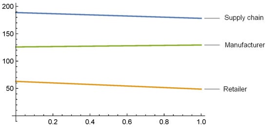
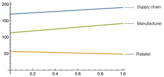
We perform some numerical analysis. In the overstocking case (i.e., $c\le c_l$), Figure 7 shows that both the chain profit and the retailer’s profit decrease with the level of overconfidence $\alpha$, mainly because the retail price decreases with the level of overconfidence by Proposition 2. In the understocking case (i.e., $c\ge c_h$), Figure 8 shows that both the chain profit and the manufacturer’s profit increase with the level of overconfidence $\alpha$ because the minimum demand is overestimated and consumers are better served.

Figure 7. The chain profit with $\alpha$ when $c\le c_l$.

Figure 8. The chain profit with $\alpha$ when $c>c_h$.

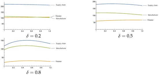
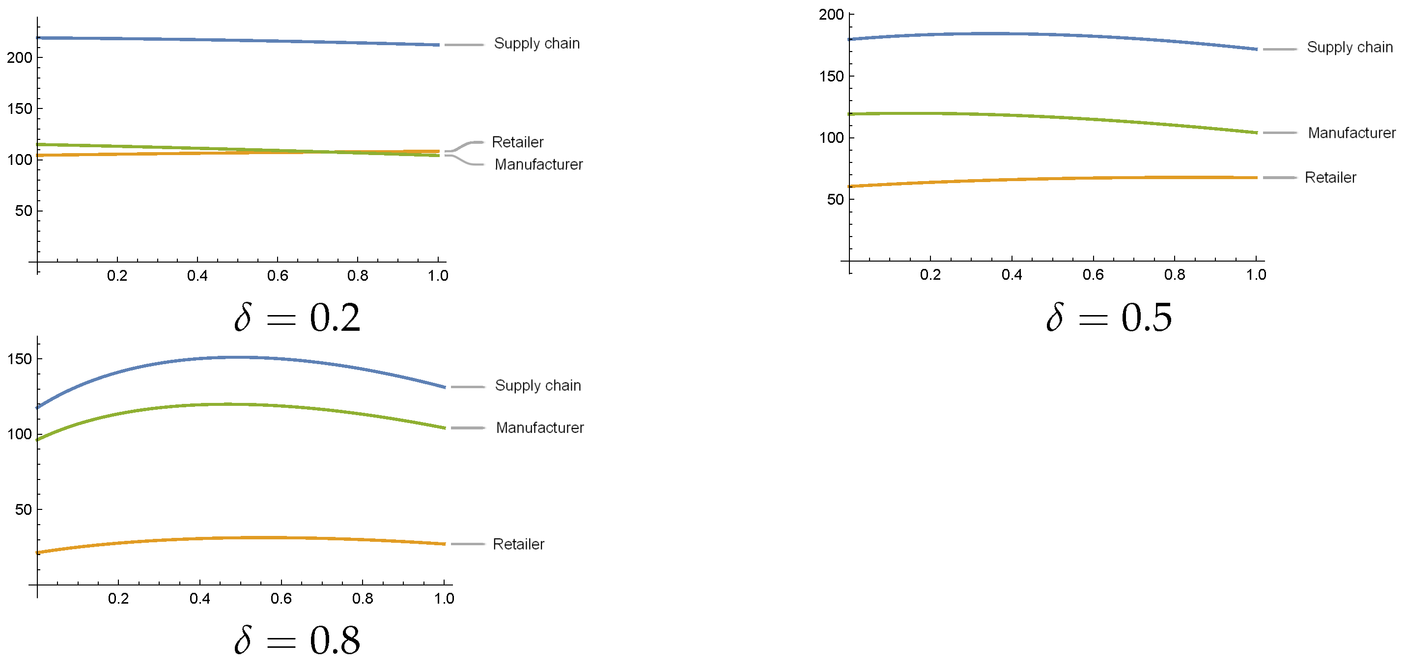
However, in the intermediate case, the situation is quite complicated, as numerically illustrated in Figure 9 with $a=35,s=0.5$ and $c=2$ for different values of $\delta$. The supply chain has the opportunity to be better because of the overconfidence. In numerical analysis, when $\delta$ is small, such as when $\delta =0.2$, the profit of the supply chain always decreases in $\alpha$, while when $\delta$ is large, such as when $\delta =0.8$, the supply chain’s profit first increases and then decreases in $\alpha$. As the volatility of the demand increases, the level of overconfidence affects the change in the supply chain’s profit more significantly.

Figure 9. The profit changes with $\alpha$ when $c_l<c\le c_h$ for different values of $\delta$.

The robustness of our results with respect to the demand specification is examined in Appendix B, where the Bernoulli distribution in (1) is replaced by a continuous uniform distribution $ϵ\sim U[1-\delta ,1+\delta ]$, which matches the Bernoulli specification in its mean ($E\left[ϵ\right]=1$) and in the endpoints of its support ($1\pm \delta$), but not in its variance: the variance of the uniform distribution is ${\delta }^2/3$, whereas that of the binary distribution is ${\delta }^2$. To rule out the possibility that the differences reported below are driven by this variance gap rather than by the change in distributional form, Appendix B additionally reports a variance-matched uniform specification, $\epsilon \sim U[1-\sqrt{3}\delta ,1+\sqrt{3}\delta ]$ (which has variance ${\delta }^2$), and shows that the conclusions are unchanged. The retailer’s equilibrium under uniform demand is fully characterized: the optimal stocking factor follows the critical fractile, the optimal price solves a cubic equation, and the manufacturer’s problem is solved numerically (Appendix B). The comparative statics deliver a clear and honest boundary of our central claim. Under continuous demand, overconfidence is unambiguously self-harming for the retailer (her realized profit is strictly decreasing in $\alpha$, ${\alpha }_1\equiv 0$) and unambiguously beneficial for the manufacturer (${\alpha }_2\equiv 1$) across the entire parameter grid: because the retailer’s order is always interior, there is no boundary-ordering threshold at which the manufacturer would concede a lower wholesale price, and the manufacturer instead exploits the retailer’s reduced price sensitivity by charging a higher wholesale price. The beneficial effect of moderate overconfidence documented in Propositions 3 and 4 is therefore specific to the binary demand structure. This interpretation is corroborated by the asymmetric binary extension in Appendix B.4, which preserves the main-text pattern (${\alpha }_1>0$ and a decreasing wholesale price in $\alpha$), showing that the symmetric probability 1/2 is not the operative assumption. In light of these findings, we state our conclusions for binary demand and emphasize that extending them to continuous-demand or multi-state environments is a promising direction for future research.

4.3. Economic Mechanism of the Win-Win Region

The results in Propositions 2–4 establish that in the intermediate regime ($c_l<c\le c_h$), a moderate level of retailer overconfidence can simultaneously increase the retailer’s, the manufacturer’s, and the integrated channel’s profits. We now decompose the channels through which this counterintuitive effect arises.

4.3.1. Four Candidate Mechanisms

We identify four candidate economic channels that could, in principle, generate a positive effect of overconfidence on chain profit.

(i)

Order-quantity channel. Overprecision causes the retailer to perceive a lower demand variance. Holding wholesale price constant, the retailer’s perceived optimal order quantity converges to the unconditional mean demand-the ‘pull-to-center’ effect. In the intermediate regime, the unbiased optimum is closer to the maximum demand; under-ordering therefore reduces the mismatch between the realized demand and the order quantity, and the salvage value recovers part of the previously wasted inventory.

(ii)

Wholesale-price channel. The manufacturer, anticipating the overconfident retailer’s reduced order elasticity (see Equation (21): $\partial q_H^{oc}/\partial w=-{\displaystyle \frac{1}{2}}{\left[1+(1-\alpha )\delta \right]}^2$ vs. the unbiased $\partial q/\partial w=-{\displaystyle \frac{1}{2}}{(1+\delta )}^2$), optimally lowers the wholesale price in the intermediate regime (Proposition 2(1)). The price concession is a strategic gift to the overconfident retailer, induced by the retailer’s behavioral bias.

(iii)

Retail-price channel. In the intermediate regime, the overconfident retailer’s optimal price $p_{oc}^{*}$ is lower than $p^{*}$ (Proposition 2(2)), which expands realized sales.

(iv)

Double-marginalization channel. A decentralized wholesale-price contract creates double marginalization (Spengler, 1950 [23]). Because overprecision partially aligns the retailer’s perceived marginal revenue with the chain-optimal one, it relaxes the wedge between decentralized and centralized decisions, reducing the double marginalization loss. Li (2019) [13] first observed this channel in the additive setting; the present paper confirms that it persists in the multiplicative setting with a stronger qualitative force.

4.3.2. Numerical Decomposition

To identify the contribution of each of the four channels defined in Section 4.3.1, we adopt a factorial counterfactual design. Two decisions determine the outcome of the game: the manufacturer’s wholesale price w and the retailer’s pair of decisions $(p,q)$. Each of these can be set at its unbiased level (the equilibrium values under $\alpha =0$) or at its overconfident level (the equilibrium values under $\alpha ={\alpha }_1(0.75)$). The baseline (row 1) sets both at the unbiased level. Row 2 reports the full-equilibrium configuration in which both are set at their overconfident levels, with all three member-level channels (i) + (ii) + (iii) active. To isolate the individual channels, row 3 sets only the retailer’s decisions at their overconfident levels while the wholesale price remains at w*, jointly capturing the demand-side channels (i) + (iii); row 4 sets only the wholesale price at its overconfident level while the retailer remains unbiased, isolating the wholesale-price channel (ii).

Because the retailer’s overconfidence simultaneously distorts their two decisions—they form a single overconfident belief ${\delta }^{\prime }=(1-\alpha )\delta$ and use it for both pricing and ordering—the joint demand-side effect (i) + (iii) is further decomposed by two additional counterfactuals that fix one of the retailer’s decisions at its unbiased level while the other is overconfident (rows 5–6 of Table 1): fixing the retail price at its unbiased level isolates the order-quantity channel (i), and fixing the order quantity at its unbiased level isolates the retail-price channel (iii). Each of rows 4–6 therefore activates a distinct subset of the member-level channels, and together rows 2–6 provide a complete identification of the three member-level mechanisms.

Table 1. Mechanism decomposition of retailer overconfidence at $(a,s,c,\delta )=(35,0.5,7,0.75)$ with $\alpha ={\alpha }_1(0.75)\approx 0.59$; the baseline row reports the absolute profit levels of the unbiased benchmark, and the centralized row reports ${\pi }_C$; all other entries are percentage changes relative to the unbiased benchmark.

Scenario	Active Channels	$\Delta {\mathit{\pi }}^{\mathit{R}}$	$\Delta {\mathit{\pi }}^{\mathit{M}}$
Baseline unbiased	—	33.42	66.85
Overconfidence, full	(i) + (ii) + (iii)	+3.02%	+3.19%
$w=w^{*}$ , retailer overconfident	(i) + (iii)	$-31.50\%$	$-26.77\%$
$w=w_{oc}^{*}$, retailer unbiased	(ii) only	+30.00%	$-1.96\%$
Order-quantity channel only	(i)	$+7.89\%$	$+3.19\%$
Retail-price channel only	(iii)	$+2.25\%$	$-1.96\%$
Centralized benchmark	removes (iv)	${\pi }^C=133.69$	DM loss $-9.40\%$

Finally, the double-marginalization channel (iv) is a chain-level construct: it measures the distance between the decentralized chain profit and the centralized (integrated) optimum. We quantify it separately by comparing the chain profit with the centralized benchmark ${\pi }^C$ (row 7 of Table 1).

The decomposition is computed at $(a,s,c,\delta )=(35,0.5,7,0.75)$, so that $\delta >2/5$ and the equilibrium lies in the intermediate regime with an interior profit-maximizing overconfidence level ${\alpha }_1(0.75)\approx 0.59$ (consistent with Proposition 3). All entries are percentage changes relative to the unbiased benchmark.

Three observations follow. First, the wholesale-price channel (ii) is the dominant positive channel for the retailer: holding the retailer’s behavior unbiased and shifting only the wholesale price to its overconfident level $w_{oc}^{*}$ raises the retailer’s profit by $+30.00\%$, whereas the order-quantity channel (i) contributes a positive but small $+7.89\%$ and the retail-price channel (iii) contributes $+2.25\%$. The dominant role of channel (ii) is also reflected in the equilibrium: $w^{*}$ decreases by $6.81\%$ (from 13.61 to 12.68), the manufacturer’s wholesale-price concession that Proposition 2(1) identifies as the operative mechanism. Second, the full effect is a win-win: at $\alpha ={\alpha }_1(0.75)$, the retailer’s and the manufacturer’s profits increase simultaneously ($+3.02\%$ and $+3.19\%$, respectively), and the chain profit rises by $+3.13\%$. Third, the channels interact nonlinearly: the isolated effects do not add up to the full effect, because when the wholesale price is held at the unbiased level while the retailer is fully overconfident (row 3, $-31.50\%$), the overconfident retailer’s joint price-and-order distortion is not compensated by any concession; in the full equilibrium, the concession channel more than offsets this distortion. The double-marginalization channel (iv) is quantified separately: relative to the centralized optimum ${\pi }^C=133.69$, the chain profit under “Overconfidence, full” is 103.41; the double-marginalization loss falls from 33.42 to 30.28, which is a reduction of $9.40\%$.

4.3.3. Why Does the Manufacturer Gain?

In the intermediate regime, the wholesale price concession is more than offset by the retailer’s order expansion induced by the perceived lower variance (Proposition 2(3): $q_{oc}^{*}$ is increasing in $\alpha$ in the relevant sub-region). The volume effect dominates the price effect, and the manufacturer captures a positive profit increment despite the lower w. This contrasts with the overstocking region, where the manufacturer gains through both higher w and higher q, and the understocking region, where w is fixed and only the volume effect operates.

4.4. Managerial Implications

The analytical results in Propositions 2–4 yield a set of model-based implications for channel management. We emphasize at the outset that these implications are conditional: they are derived within the two-echelon, single-period, wholesale-price setting with Bernoulli demand and the variance-reducing overprecision representation of Section 3.1, and they have not been empirically validated. We therefore phrase them as tendencies suggested by the model, to be confirmed under the institutional and informational conditions of the focal supply chain, rather than as universal prescriptions.

(1)

For the manufacturer. The model indicates that the manufacturer’s profit is increasing in the retailer’s overconfidence level in the overstocking and understocking regimes ($c\le c_l$ and $c>c_h$), and increasing up to ${\alpha }_2(\delta )$ in the intermediate regime. Under the model’s assumptions, this suggests that, all else equal, a manufacturer selecting distribution partners could benefit from a partner with a moderate degree of overconfidence, and that debiasing an overconfident partner is not obviously profitable—an insight that runs against the conventional prescription of eliminating behavioral biases (Ancarani & Di Mauro, 2016 [22]). In the intermediate regime with excessive overconfidence ($\alpha >{\alpha }_2(\delta )$), the model predicts a decline in the manufacturer’s profit; a menu of wholesale-price contracts that incentivizes more rational ordering could in principle address this region, although the design and welfare effects of such contracts are beyond the scope of the present analysis.

(2)

For the retailer. The model shows that overconfidence is self-harming in the overstocking and understocking regimes and beneficial only in the intermediate regime with $\alpha \le {\alpha }_1(\delta )$. To the extent that a retailer cannot eliminate their bias, the model suggests two ways of mitigating its cost: in the understocking regime, ordering fewer units would reduce the inventory–demand mismatch; in the overstocking regime, committing to smaller orders in negotiations would tend to elicit a lower wholesale price from the manufacturer. In the intermediate regime, the model predicts that a small degree of overconfidence is profit-maximizing for the retailer, implying that the conventional bias-elimination prescription is not strictly optimal in this region. Whether these adjustments remain desirable in practice—where forecasting systems, contract menus, and competitive interactions differ from the model—requires empirical assessment.

(3)

For contract design. The analysis identifies the channel through which overconfidence affects contracting: the overconfident retailer’s reduced price sensitivity induces a wholesale-price concession, which is the main driver of the win-win region (Section 4.3). Within the model, this suggests that simple wholesale-price contracts may suffice to align incentives when the retailer is moderately overconfident, whereas more complex contracts (revenue sharing, two-part tariffs) could become relevant mainly when overconfidence is excessive. Extending the analysis to such contracts is identified as a promising direction.

5. Conclusions

This paper explores how an overconfident retailer influences the supply chain. The retailer inaccurately forecasts the demand because of their overconfidence, which affects their decisions and, in turn, the manufacturer’s decisions. We have several main findings.

First, the equilibrium falls into three regimes-overstocking, intermediate, and understocking-depending on the production cost, and the retailer’s level of overconfidence affects the pricing and ordering decisions in a regime-dependent way (Propositions 1–2). Second, the retailer is not always worse off with overconfidence: in the intermediate regime with a moderate production cost and demand volatility not too high, their profit first increases and then decreases with the level of overconfidence, so that an optimal, strictly positive degree of overconfidence ${\alpha }_1(\delta )$ exists (Proposition 3). Third, the manufacturer generally benefits from retailer overconfidence except in the intermediate regime with excessive overconfidence (Proposition 4), and a win-win region exists in which moderate overconfidence raises the profits of both channel members and the integrated chain.

This paper extends the behavioral operations literature on overconfidence in three ways: (i) it moves the analysis from additive to multiplicative demand, where the price scales demand variance and overprecision alters the retailer’s price sensitivity; (ii) it identifies a win-win region and interior optimal overconfidence levels that do not arise under additive demand (Li, 2019 [13]); and (iii) it provides a mechanism decomposition showing that the manufacturer’s strategic wholesale price concession is the dominant driver of the beneficial effect.

For manufacturers, the model indicates that the manufacturer’s profit is generally increasing in the retailer’s overconfidence level, except in the intermediate regime with excessive overconfidence, where the model predicts a decline; a manufacturer could therefore benefit from a moderately overconfident retail partner, and debiasing interventions are not obviously profitable within the model’s conditions. For retailers, the model predicts that overconfidence is self-harming in the extreme regimes—ordering fewer units would mitigate the loss—whereas in the intermediate regime a small degree of overconfidence is profit-maximizing. For contract design, the wholesale-price concession is identified as the channel through which overconfidence relaxes double marginalization, suggesting that simple wholesale-price contracts may perform adequately with moderately overconfident retailers; whether these implications carry over to other contractual, informational, and competitive environments requires empirical validation.

5.1. Boundary Conditions and Limitations

The present results should be interpreted within the following boundaries:

(i)

The supply chain is a two-echelon channel (one manufacturer, one retailer). The chain profit is the sum of these two parties’ profits.

(ii)

The contract is a wholesale-price contract. Other contracts (revenue sharing, two-part tariff, buyback) may yield qualitatively different patterns.

(iii)

Demand uncertainty is idiosyncratic and single-period. Inter-temporal demand dynamics, forecast updating across periods, and information propagation through multiple echelons are not modeled.

(iv)

The retailer is overconfident but the manufacturer is rational. Symmetric or bilateral overconfidence is outside the scope.

(v)

The overconfidence representation is the variance-reducing, mean-preserving contraction ${ϵ}^{oc}=\alpha \mu +(1-\alpha )ϵ$. Alternative operationalizations (e.g., overestimation of demand level, miscalibration of the entire distribution shape) may yield different results.

These conclusions are internal to the model: they follow from the analytical and numerical results under the specified parameter values. Translating them into managerial prescriptions for real supply chains requires (i) empirical validation in field or experimental settings, (ii) recognition of the contract and information-sharing environment of the focal firm, and (iii) acknowledgment that the present model does not capture inter-temporal learning, multi-echelon propagation, or competitive interaction among retailers. We therefore frame our managerial implications as conditional rather than universal statements.

In short, the analysis identifies a theoretically possible and mechanically explicable region in which overprecision is not uniformly detrimental, but the practical relevance of the finding should be assessed in conjunction with the institutional and informational characteristics of the focal supply chain.

5.2. Future Research

(a)

Dynamic learning and AI-enabled debiasing. The present model assumes that $\alpha$ is exogenous and stable. In practice, retailers operating with AI-driven demand forecasting systems (Salinas et al., 2020 [24]; Islam, Hassanzadeh Amin and Wardley 2024 [25]) or with real-time point-of-sale data sharing (Walmart’s Retail Link is the canonical case) can update their perceived demand distribution in light of repeated forecast errors. A natural extension is to model ${\alpha }_t$ as a state variable that evolves according to a Bayesian or reinforcement-learning rule, and to study the conditions under which the beneficial effect of moderate overconfidence survives a debiasing trajectory.

(b)

Information sharing. When the manufacturer and retailer share real-time demand information (e.g., via Vendor-Managed Inventory, CPFR, or blockchain-based traceability), the retailer’s perceived variance will move closer to the truth. Studying how the win-win region shifts under different information-sharing regimes is a natural next step.

(c)

Multi-echelon extension. As discussed in Section 2, the relationship between the retailer’s overprecision and upstream propagation is a behavioral bullwhip question recently studied by Zhou et al. (2025) [18]. Embedding our wholesale-price response mechanism in a multi-echelon setting is a logical extension.

(d)

Alternative contracts and behavioral heterogeneity. The present analysis assumes a wholesale-price contract and unilateral retailer overconfidence. Extending to revenue-sharing, two-part tariffs, and buyback contracts, as well as to bilateral or competing-retailer overconfidence, will determine whether the win-win region survives in richer contractual and competitive environments.

Appendix A.1. Proof of Lemma 1

Proof of Lemma 1.

Firstly, note that ${\pi }_r(p)$ is a piecewise function and is continuous in p for $p\in (w,a)$. For ease of exposition, we define ${\pi }_r^L$ and ${\pi }_r^H$ as the two pieces in the expression of ${\pi }_r(p)$, i.e.,

$$\begin{array}{cc}\hfill {\pi }_r^L=& (1-\delta )(a-p)(p-w),\hfill \\ \hfill {\pi }_r^H=& (a-p)[p-w-\delta (w-s)].\hfill \end{array}$$

Both ${\pi }_r^L$ and ${\pi }_r^H$ are quadratic functions of p. It is easy to prove that ${\pi }_r^L(p)$ increases in $p\in (w,{\displaystyle \frac{1}{2}}(a+w)]$ but decreases in $p\in ({\displaystyle \frac{1}{2}}(a+w),a)$. Also, ${\pi }_r^H(p)$ increases in $p\in \left(w,{\displaystyle \frac{1}{2}}[a+w+\delta (w-s)]\right]$ and decreases in $p\in ({\displaystyle \frac{1}{2}}[a+w+\delta (w-s)],a)$.

We characterize the optimal retail price by considering the following three cases based on the value of w.

Case 1: $w<{\displaystyle \frac{a+2s}{3}}$.

In this case, ${\displaystyle \frac{1}{2}}[a+w+\delta (w-s)]>{\displaystyle \frac{1}{2}}(a+w)>2w-s$. Then, for $p\in (w,2w-s]$, ${\pi }_r(p)={\pi }_r^L(p)$ is increasing. For $p\in \left[2w-s,{\displaystyle \frac{1}{2}}[a+w+\delta (w-s)]\right]$, ${\pi }_r^H(p)$ is increasing, but for $p\in ({\displaystyle \frac{1}{2}}[a+w+\delta (w-s)],a]$, ${\pi }_r(p)={\pi }_r^H(p)$ is decreasing. So the optimal value of ${\pi }_r$ is achieved at $p={\displaystyle \frac{1}{2}}[a+w+\delta (w-s)]$.

Case 2: $w>{\displaystyle \frac{a+(2-\delta )s}{3-\delta }}$.

In this case, ${\displaystyle \frac{1}{2}}(a+w)<{\displaystyle \frac{1}{2}}[a+w+\delta (w-s)]<2w-s$. Then, ${\pi }_r(p)={\pi }_r^L(p)$ is increasing in $p\in [w,{\displaystyle \frac{1}{2}}(a+w)]$, but decreasing in $p\in ({\displaystyle \frac{1}{2}}(a+w),2w-s]$. Moreover, ${\pi }_r(p)={\pi }_r^H(p)$ is decreasing in $p\in (2w-s,a]$. So, the optimal value of ${\pi }_r$ is achieved at $p={\displaystyle \frac{1}{2}}(a+w)$.

Case 3: ${\displaystyle \frac{a+2s}{3}}\le w\le {\displaystyle \frac{a+(2-\delta )s}{3-\delta }}$.

In this case, ${\displaystyle \frac{1}{2}}(a+w)\le 2w-s\le {\displaystyle \frac{1}{2}}[a+w+\delta (w-s)]$. Then ${\pi }_r(p)={\pi }_r^L(p)$ is increasing in $p\in [w,{\displaystyle \frac{1}{2}}(a+w)]$, and decreasing in $p\in ({\displaystyle \frac{1}{2}}(a+w),2w-s]$. ${\pi }_r(p)={\pi }_r^H(p)$ is increasing in $p\in [2w-s,{\displaystyle \frac{1}{2}}[a+w+\delta (w-s)]]$, but is decreasing in $p\in ({\displaystyle \frac{1}{2}}[a+w+\delta (w-s)],a]$. So, the maximized profit of ${\pi }_r(p)$ in $p\in [s,2w-s]$ is achieved at $p={\displaystyle \frac{1}{2}}(a+w)$; the maximized profit of ${\pi }_r(p)$ in $p\in [2w-s,a]$ is achieved at $p={\displaystyle \frac{1}{2}}[a+w+\delta (w-s)]$.

To derive the best retail price, it is sufficient to compare the retailer’s profits at these two points:

$$\begin{array}{cc}\hfill \Delta {\pi }_r(w)& ={\pi }_r^H\left({\displaystyle \frac{1}{2}}[a+w+\delta (w-s)]\right)-{\pi }_r^L\left({\displaystyle \frac{1}{2}}(a+w)\right)\hfill \\ \hfill & ={\displaystyle \frac{1}{4}}{[a+\delta s-(1+\delta )w]}^2-{\displaystyle \frac{1}{4}}(1-\delta ){(a-w)}^2\hfill \\ \hfill & ={\displaystyle \frac{1}{4}}\delta [(3+\delta )w^2-2(2a+s+\delta s)w+a^2+2as+\delta s^2].\hfill \end{array}$$

$\Delta {\pi }_r(w)$ is a quadratic function of w, opening upward. In addition, $\Delta {\pi }_r({\displaystyle \frac{a+2s}{3}})\ge 0$ and $\Delta {\pi }_r({\displaystyle \frac{a+(2-\delta )s}{3-\delta }})\le 0$. So, there is a unique solution to $\Delta {\pi }_r(w)=0$ in the interval $[{\displaystyle \frac{a+2s}{3}},{\displaystyle \frac{a+(2-\delta )s}{3-\delta }}]$. Solving $\Delta {\pi }_r(w)=0$ for w, we obtain the smaller root $w=w_0$, as defined in (4).

It follows that for $w\in [{\displaystyle \frac{a+2s}{3}},w_0)$, $\Delta {\pi }_r(w)\ge 0$, that is, ${\pi }_r^H\left({\displaystyle \frac{1}{2}}[a+w+\delta (w-s)]\right)\ge {\pi }_r^L\left[{\displaystyle \frac{1}{2}}(a+w)\right]$ (the equality holds only when $\delta =0$). Therefore, the optimal value of ${\pi }_r$ is achieved at $p={\displaystyle \frac{1}{2}}[a+w+\delta (w-s)]$. Otherwise, when $w\in (w_0,{\displaystyle \frac{a+(2-\delta )s}{3-\delta }}]$, the optimal value of ${\pi }_r$ is achieved at $p={\displaystyle \frac{1}{2}}(a+w)$.

When $w=w_0$, the retailer is indifferent to these two prices. For ease of exposition, we assume that the retailer will choose $p={\displaystyle \frac{1}{2}}[a+w+\delta (w-s)]$ when $w=w_0$.

Combining the three cases above together, we proved Lemma 1. □

Appendix A.2. Proof of Lemma 2

Proof of Lemma 2.

It suffices to show $f_2(\delta )-f_1(\delta )>0$. Note that

$$\begin{array}{cc}\hfill & f_2(\delta )-f_1(\delta )\hfill \\ \hfill =& {\displaystyle \frac{-\sqrt{\delta (3+\delta )(1-\delta )}}{(1-\delta )(1+\delta )(3+\delta )}}\left[\sqrt{\delta (3+\delta )}(\sqrt{1-\delta }+2+2\delta )-2(1+\delta )\sqrt{(1+\delta +\sqrt{1-\delta })(1+\delta )}\right].\hfill \end{array}$$

(A1)

It is obvious that the fractional part of Equation (A1) is negative for $\delta \in (0,1)$. Hence, it suffices to show that the term in the brackets is also negative for $\delta \in (0,1)$, which is equivalent to

$${\displaystyle \frac{\sqrt{\delta (3+\delta )}}{1+\delta }}<{\displaystyle \frac{2\sqrt{(1+\delta +\sqrt{1-\delta })(1+\delta )}}{\sqrt{1-\delta }+2+2\delta }}$$

(A2)

for $\delta \in (0,1)$. For ease of exposition, let $d_1(\delta )$ and $d_2(\delta )$ be the left and right sides of the above inequality, respectively, i.e.,

$$\begin{array}{cc}\hfill d_1(\delta )=& {\displaystyle \frac{\sqrt{\delta (3+\delta )}}{1+\delta }},\hfill \\ \hfill d_2(\delta )=& {\displaystyle \frac{2\sqrt{(1+\delta +\sqrt{1-\delta })(1+\delta )}}{\sqrt{1-\delta }+2+2\delta }}.\hfill \end{array}$$

Their derivatives are, respectively,

$$\begin{array}{cc}\hfill {\displaystyle \frac{\partial d_1(\delta )}{\partial \delta }}=& {\displaystyle \frac{3-\delta }{2{(1+\delta )}^2\sqrt{\delta (3+\delta )}}}>0,\hfill \\ \hfill {\displaystyle \frac{\partial d_2(\delta )}{\partial \delta }}=& {\displaystyle \frac{3-\delta }{2\sqrt{(1+\delta )(1+\delta +\sqrt{1-\delta })}{(2+2\delta +\sqrt{1-\delta })}^2}}>0.\hfill \end{array}$$

For $\delta \in [0,1]$, $\sqrt{(1+\delta )(1+\delta +\sqrt{1-\delta })}>\sqrt{\delta (3+\delta )}$ and ${(2+2\delta +\sqrt{1-\delta })}^2>{(1+\delta )}^2$, so $\partial d_1/\partial \delta >\partial d_2/\partial \delta >0$. So, both $d_1(\delta )$ and $d_2(\delta )$ are increasing in $\delta \in (0,1)$ and $d_1(\delta )$ increases faster than $d_2(\delta )$. In addition, $d_1(0)=0$, $d_2(0)={\displaystyle \frac{2}{3}}\sqrt{2}$, and $d_1(1)=d_2(1)=1$. If there is some $\delta \in (0,1)$ satisfying $d_1(\delta )\ge d_2(\delta )$, then $d_1(1)>d_2(1)$. This is contrary to $d_1(1)=d_2(1)=1$. So, $d_1(\delta )<d_2(\delta )$ for all $\delta \in (0,1)$. Thus, from (9), $f_1(\delta )<f_2(\delta )$ for all $\delta \in (0,1)$. □

Appendix A.3. Proof of Lemma 3

Proof of Lemma 3.

From (7), we first search for the optimal solution of ${\pi }_m(w)$ in $w\ge w_0$ and $w\le w_0$, respectively. For the case of $w>w_0$, ${\pi }_m(w)={\displaystyle \frac{1}{2}}(1-\delta )(w-c)(a-w)$. Solving the first-order condition yields $w_1=(a+c)/2$. It is easy to see $w_0\le (a+s)/2<(a+c)/2$. So, the optimal solution of ${\pi }_m(w)$ in $w>w_0$ is $w_1=(a+c)/2$.

Next, for the case of $w\le w_0$, ${\pi }_m(w)=(1+\delta )(w-c)\left[a-w-\delta (w-s)\right]/2$. Solving the first-order condition for w yields $w_2=(c+{\displaystyle \frac{a+\delta s}{1+\delta }})/2$. It is easy to see that ${\pi }_m(w)$ is concave. So, when $w_2<w_0$, ${\pi }_m(w)$ is increasing in $w\in [c,w_2]$ but decreasing in $w\in [w_2,w_0]$ and so the optimal solution of ${\pi }_m(w)$ in $w\le w_0$ is $w_2$. When $w_2\ge w_0$, ${\pi }_m(w)$ is increasing in $w\in [c,w_0]$ and so the optimal solution of ${\pi }_m(w)$ in $w\le w_0$ is $w_0$.

Note that $w_2>w_0$ is equivalent to $c>f_2(\delta )a+[1-f_2(\delta )]s$, i.e., $c>c_1$. Then, we characterize the optimal wholesale price for the manufacturer in the following two cases.

Case 1: $c>c_1$.

From the above analysis, we know that in this case the optimal value of ${\pi }_m(w)$ in $w\in (c,w_0]$ is $w_0$, and that in $w\in (w_0,a]$ is $w_1$. Then, we only compare ${\pi }_m(w_0)$ with ${\pi }_m(w_1)$ as follows:

$$\begin{array}{cc}\hfill \Delta {\pi }_m=& {\pi }_m(w_1)-{\pi }_m(w_0)\hfill \\ \hfill =& {\displaystyle \frac{1}{8}}(1-\delta ){(a-c)}^2+{\displaystyle \frac{(1+\delta )(a-s)}{2{(3+\delta )}^2}}\left[1+\sqrt{1-\delta }+\delta (-1+\sqrt{1-\delta })\right]\hfill \\ \hfill & ·\left[a(-2+\sqrt{1-\delta })+c(3+\delta )-(1+\sqrt{1-\delta }+\delta )s\right].\hfill \end{array}$$

We can see that $\Delta {\pi }_m$ is a quadratic function of c, opening upward, and $\Delta {\pi }_m=0$ has two roots $c_2$ and $c_1$, as defined by (9). Moreover,

$${\displaystyle \frac{\partial \Delta {\pi }_m}{\partial c}}{|}_{c=a}={\displaystyle \frac{(1+\delta )[1+\sqrt{1-\delta }-(1-\sqrt{1-\delta })\delta ](a-s)}{2(3+\delta )}}$$

It is easy to prove that $1+\sqrt{1-\delta }>(1-\sqrt{1-\delta })\delta$ for $\delta \in [0,1]$, and so ${\displaystyle \frac{\partial \Delta {\pi }_m}{\partial c}}{|}_{c=a}>0$. Also,

$${\displaystyle \frac{\partial \Delta {\pi }_m}{\partial c}}{|}_{c=s}={\displaystyle \frac{\sqrt{1-\delta }[2{(1+\delta )}^2-(1-\delta )\sqrt{1-\delta }](a-s)}{4(3+\delta )}}\ge 0$$

because $2{(1+\delta )}^2-(1-\delta )\sqrt{1-\delta }>0$ for $\delta$. By the assumption of $s<c<a$, the larger root of $\Delta {\pi }_m(c)=0$, i.e., $c_2$ defined in Equation (9), determines the sign of $\Delta {\pi }_m$.

Hence, when $c_1<c\le c_2$, we have ${\pi }_m(w_1)\le {\pi }_m(w_0)$. Then, the optimal wholesale price for the manufacturer is $w_0$.

When $c>c_2$, we have ${\pi }_m(w_1)>{\pi }_m(w_0)$. Then, the optimal wholesale price for the manufacturer is $w_1$.

Case 2: $c\le c_1$

In this case, the optimal solution of ${\pi }_m(w)$ in $w\in (c,w_0]$ is $w_2$, and that in $w\in (w_0,a]$ is still $w_1$. Consequently, we have ${\pi }_m(w_2)>{\pi }_m(w_0)$. It is obvious that $c\le c_1\le c_2$ and ${\pi }_m(w_1)\le {\pi }_m(w_0)$. So, ${\pi }_m(w_2)>{\pi }_m(w_0)\ge {\pi }_m(w_1)$. Thus, the optimal wholesale price for the manufacturer is $w_2$.

Overall, the optimal wholesale price is given by (10). □

Appendix A.4. Proof of Proposition 1

Proof of Proposition 1.

The property of $w^{*}$ is true due to ${\displaystyle \frac{\partial w^{*}}{\partial \delta }}={\displaystyle \frac{s-a}{2{(1+\delta )}^2}}<0$ for $c<c_1$ and ${\displaystyle \frac{\partial w^{*}}{\partial \delta }}=-{\displaystyle \frac{\left(\delta +4\sqrt{1-\delta }-5\right)(a-s)}{2\sqrt{1-\delta }{(\delta +3)}^2}}>0$ for $c\in (c_1,c_2)$. Similarly, we can prove the property of $p^{*}$.

For the property of $q^{*}$, for $c\le c_1$, ${\displaystyle \frac{\partial q^{*}}{\partial \delta }}=a+\delta (2s-2c)-2c+s$ and ${\displaystyle \frac{{\partial }^2{q}^{*}}{\partial {\delta }^2}}=-\delta (2c-2s)<0$. So, $q^{*}$ is concave and is increasing in $\delta <{\displaystyle \frac{a-2c+s}{2(c-s)}}$ while decreasing in $\delta >{\displaystyle \frac{a-2c+s}{2(c-s)}}={\delta }_1^{*}$. Notice that when $a>4c-3s$, ${\displaystyle \frac{a-2c+s}{2(c-s)}}>1$ and so $q^{*}$ always increases in $\delta$ for $c<c_1$.

For $c\in (c_1,c_2]$, we let $x=\sqrt{1-\delta }$. Then, $\delta =1-x^2$ and as a function of x we have $q^{*}={\displaystyle \frac{a-s}{2(2+x)}}(x+x^2)(2-x^2)$. So, ${\displaystyle \frac{\partial q^{*}}{\partial x}}={\displaystyle \frac{a-s}{2{(2+x)}^2}}\{4+8x-4x^2-10x^3-3x^4\}$ after some algebraic computations. Thus, it can be proved that there is some $x^{*}\in (0,1)$ such that ${\displaystyle \frac{\partial q^{*}}{\partial x}}>0$ for $x<x^{*}$ and $<0$ for $x>x^{*}$. This implies that there is some ${\delta }_2^{*}\in (0,1)$ such that ${\displaystyle \frac{\partial q^{*}}{\partial \delta }}>0$ for $\delta <{\delta }^{*}$ and $<0$ for $\delta >{\delta }^{*}$. □

Appendix A.5. Proof of Proposition 3

Proof of Proposition 3.

(1) When $c\in [s,c_l)$, from Equation (19),

$$\begin{array}{cc}\hfill {\displaystyle \frac{\partial {\pi }_{roc}^{*}(\alpha )}{\partial \alpha }}=& {\displaystyle \frac{1}{32}}\delta (-3a^2+6ac-3c^2+2ac\delta -2c^2\delta +c^2{d}^2-2a\delta s+2c\delta s-2c{d}^{2}s+d^2{s}^2)\hfill \\ \hfill & +{\displaystyle \frac{1}{32}}\delta (-4ac\delta -4c^2{d}^2+4a\delta s+4c\delta s+8c{d}^{2}s-4\delta s^2-4d^2{s}^2)\alpha \hfill \\ \hfill & +{\displaystyle \frac{1}{32}}\delta \left[3{\delta }^2{(c-s)}^2\right]{\alpha }^2\hfill \end{array}$$

(A3)

which is obviously a quadratic function of $\alpha$, opening upward. Moreover,

$$\begin{array}{cc}\hfill {\displaystyle \frac{\partial {\pi }_{roc}^{*}(\alpha )}{\partial \alpha }}{|}_{\alpha =0}=& {\displaystyle \frac{1}{32}}\delta (-3a^2+6ac-3c^2+2ac\delta -2c^2\delta +c^2{d}^2-2a\delta s+2c\delta s-2c{d}^{2}s+d^2{s}^2)<0,\hfill \\ \hfill {\displaystyle \frac{\partial {\pi }_{roc}^{*}(\alpha )}{\partial \alpha }}{|}_{\alpha =1}=& {\displaystyle \frac{1}{32}}\delta \{-3a^2+c^2(-3-2d)+6c\delta s-4\delta s^2+a[c(6-2d)+2\delta s]\}<0.\hfill \end{array}$$

(A4)

Hence, ${\pi }_{roc}^{*}(\alpha )$ is decreasing in $\alpha$.

(2) When $c\ge c_h$, again from Equation (19),

$${\displaystyle \frac{\partial {\pi }_{roc}^{*}(\alpha )}{\partial \alpha }}=-{\displaystyle \frac{1}{32}}(a-c)(a\delta +3c\delta -4\delta s)<0.$$

Hence, ${\pi }_{roc}^{*}(\alpha )$ is decreasing in $\alpha$ for $c\ge c_h$.

(3) When $c\in [c_l,c_h)$, again from Equation (19),

$$\begin{array}{cc}\hfill & {\pi }_{roc}^{\prime }(\alpha )=\hfill \\ \hfill & -{\displaystyle \frac{{(a-s)}^2\delta [{\alpha }^2{\delta }^2+2\alpha \delta \left(2\sqrt{1-(1-\alpha )\delta }-\delta +1\right)-(\delta +1)\left(\sqrt{1-(1-\alpha )\delta }-\delta +1\right)]}{4\sqrt{1-(1-\alpha )\delta }{\left(\sqrt{1-(1-\alpha )\delta }+2\right)}^3}}\hfill \end{array}$$

(A5)

and

$$\begin{array}{cc}\hfill {\pi }_{roc}^{″}(\alpha )=& -{\displaystyle \frac{1}{8{(2+\sqrt{1+\delta (-1+\alpha )})}^2}}{(a-s)}^2\{-4[1+\sqrt{1+\delta (-1+\alpha )}]\hfill \\ \hfill & +\delta [6+4\sqrt{1+\delta (-1+\alpha )}-2\alpha ]+{\delta }^3(-2+\alpha ){(-1+\alpha )}^2+3{\delta }^2(-1+\alpha )\alpha \}.\hfill \end{array}$$

(A6)

It is easy to see that ${\pi }_{roc}^{{*}^{″}}(\alpha )<0$. So, ${\pi }_{roc}^{{*}^{\prime }}(\alpha )$ is decreasing in $\alpha$. Moreover, ${\pi }_{roc}^{{*}^{\prime }}{(\alpha )|}_{\alpha =0}={\displaystyle \frac{\delta (\delta +1)(\sqrt{1-\delta }-\delta +1){(a-s)}^2}{4\sqrt{1-\delta }{\left(\sqrt{1-\delta }+2\right)}^3}}>0$ and ${\pi }_{roc}^{{*}^{\prime }}{(\alpha )|}_{\alpha =1}={\displaystyle \frac{\delta }{108}}(2-5\delta ){(a-s)}^2$. This implies that there is a unique ${\alpha }_1(\delta )$ such that ${\pi }_{roc}^{{*}^{\prime }}(\alpha )>0$ for $\alpha <{\alpha }_1(\delta )$ and ${\pi }_{roc}^{{*}^{\prime }}(\alpha )<0$ for $\alpha >{\alpha }_1(\delta )$, that is, ${\pi }_{roc}^{*}(\alpha )$ increases for $\alpha <{\alpha }_1(\delta )$ but decreases for $\alpha >{\alpha }_1(\delta )$. Especially, when $\delta \le {\displaystyle \frac{2}{5}}$, ${\displaystyle \frac{\partial {\pi }_{roc}^{*}(\alpha )}{\partial \alpha }}{|}_{\alpha =1}>0$, so ${\displaystyle \frac{\partial {\pi }_{roc}^{*}(\alpha )}{\partial \alpha }}>0$ for all $\alpha \in [0,1]$, and thus ${\alpha }_1(\delta )=1$. □

Appendix A.6. Proof of Proposition 4

Proof of Proposition 4.

 

First, we have ${\pi }_{moc}^{*}(\alpha )=(w_{oc}^{*}-c)q_{oc}^{*}(w_{oc}^{*})$.

(1) When $c\in [s,c_l]$, ${\pi }_{moc}^{*}(\alpha )={\displaystyle \frac{1}{8}}{[a-c-(1-\alpha )\delta (c-s)]}^2$, which is increasing in $\alpha$ due to $c>s$. When $c\ge c_h$, ${\pi }_{moc}^{*}(\alpha )={\displaystyle \frac{1}{8}}[1-(1-\alpha )\delta ]{(a-c)}^2$, which is obviously increasing in $\alpha$.

(2) When $c\in (c_l,c_h]$, ${\pi }_{moc}^{*}(\alpha )=g_m\left[(1-\alpha )\delta \right]$, where

$$g_m(\delta )={\displaystyle \frac{(1+\sqrt{1-\delta }-\delta )(1+\delta )(a-s)[a-(2+\sqrt{1-\delta })c+s+\sqrt{1-\delta }s]}{2{(2+\sqrt{1-\delta })}^2}}.$$

(A7)

Let $x=\sqrt{1-\delta }$. Then $\delta =1-x^2$ and so

$$g_m^{*}(x):=g_m(1-x^2)={\displaystyle \frac{(a-s)(2-x^2)(x+x^2)[a+s(1+x)-c(2+x)]}{2{(2+x)}^2}}$$

(A8)

For the monotonicity of $g_m^{*}(x)$, we have

$$\begin{array}{cc}\hfill & {\displaystyle \frac{\partial g_m^{*}(x)}{\partial x}}\hfill \\ \hfill =& -{\displaystyle \frac{a-s}{2{(2+x)}^3}}\{a(2x^2+x-2)[2+x(4+x)]+s(1+x)[x(5+3x)(x^2+2x-2)-4]\hfill \\ \hfill & +c[8-x(x^2+2x-2)(10+10x+3x^2)]\}\hfill \\ \hfill =& -{\displaystyle \frac{a-s}{2{(2+x)}^3}}h(x)\hfill \end{array}$$

(A9)

where $h(x)=(2x^4+9x^3+6x^2-6x-4)a+(3x^5+14x^4+15x^3-6x^2-14x-4)s-(3x^5+16x^4+24x^3-20x-8)c$. Now,

$$\begin{array}{cc}\hfill h^{\prime }(x)=& (8x^3+27x^2+12x-6)a+(15x^4+56x^3+45x^2-12x-14)s\hfill \\ \hfill & -(15x^4+64x^3+72x^2-20)c,\hfill \\ \hfill h^{″}(x)=& (24x^2+54x+12)a+(60x^3+168x^2+90x-12)s-(60x^3+192x^2+144x)c,\hfill \\ \hfill h^{‴}(x)=& (48x+54)a+(180x^2+336x+90)s-(180x^2+384x+144)c\hfill \\ \hfill =& -180(c-s)x^2+(48a+336s-384c)x+54a+90s-144c.\hfill \end{array}$$

(A10)

Hence, $h^{‴}(x)$ is concave with $h^{‴}(0)=54a+90s-144c$ and $h^{‴}(1)=102a+606s-708c$. Since a is the scale of the market and c is the unit cost, a is sufficiently large relative to c such that $h^{‴}(0)>0$ and $h^{‴}(1)>0$. Then, $h^{‴}(x)>0$.

Hence, $h^{″}(x)$ is increasing in $x\in [0,1]$. Now, $h^{″}(0)=12(a-s)>0$ and so $h^{″}(x)>0$ for all x. This implies that $h^{\prime }(x)$ is increasing. Since $h^{\prime }(0)=-6a-14s+20c<0$ while $h^{\prime }(1)=41a+90s-131c>0$ for large enough a, there is a unique $x_0\in (0,1)$ such that $h^{\prime }(x)<0$ for $x\in [0,x_0)$, $h^{\prime }(x_0)=0$, and $h^{\prime }(x)>0$ for $x\in (x_0,1]$.

Therefore, $h(x)$ is decreasing in $x\in [0,x_0)$ but increasing in $x\in (x_0,1]$. Now, $h(0)=-4a-4s+8c<0$ and $h(1)=7a+8s-15c>0$ for large enough a. So, there is a unique $x^{*}\in (x_0,1)$ such that $h(x)<0$ for $x<x^{*}$ but $h(x)>0$ for $x>x^{*}$. Note that a represents the base market size of the product, c is the cost of the product, and s is the salvage value of the product. Thus, a is much larger than s and c and so it is adequate to have $-4a-4s+8c<0$ and $7a+8s-15c>0$.

So, ${\displaystyle \frac{\partial g_m^{*}(x)}{\partial x}}>0$ for $x<x^{*}$ but ${\displaystyle \frac{\partial g_m^{*}(x)}{\partial x}}<0$ for $x>x^{*}$. This implies that $g_m^{*}(x)$ is increasing in $x\in [0,x^{*}]$ but decreasing in $x\in [x^{*},1]$. Since ${\pi }_{moc}^{*}(\alpha )=g_m((1-\alpha )\delta )=g_m^{*}(\sqrt{1-(1-\alpha )\delta })$, we conclude that ${\pi }_{moc}^{*}(\alpha )$ is increasing in $\alpha \le {\alpha }_2(\delta ):={\displaystyle \frac{1}{\delta }}({(x^{*})}^2+\delta -1)$ but is decreasing in $\alpha \ge {\alpha }_2(\delta )$. Here, ${\alpha }_2(\delta )\le 1$, but ${\alpha }_2(\delta )\ge 0$ if and only if $\delta \ge 1-{(x^{*})}^2$. Especially, when $\delta \le 1-{(x^{*})}^2$, ${\pi }_{moc}^{*}(\alpha )$ is decreasing in $\alpha$. □

Appendix B.1. Uniform-Demand Robustness Analysis

This appendix checks whether the central results of the paper survive when the Bernoulli specification in (1) is replaced by a continuous uniform distribution of the market intensity, $\epsilon \sim U[1-\delta ,1+\delta ]$, $\delta \in [0,1]$, with $E\left[\epsilon \right]=1$. The overconfidence representation is unchanged: the retailer perceives ${\epsilon }^{oc}=\alpha \mu +(1-\alpha )\epsilon$, $\mu =1$, i.e., a uniform distribution with volatility ${\delta }^{\prime }=(1-\alpha )\delta$. All other elements of the model in Section 3.1 are retained. We report the derivation of the retailer’s equilibrium, the numerical solution of the manufacturer’s problem, and the resulting comparative statics in $\alpha$.

The support-endpoint matching is the natural benchmark for this robustness exercise: in the Bernoulli specification (1) the parameter $\delta$ is defined by the two demand states $1\pm \delta$, and the variance ${\delta }^2$ is only a derived quantity. Replacing the Bernoulli by a continuous distribution while keeping the endpoints $1\pm \delta$ fixed therefore preserves the economic meaning of $\delta$ (the amplitude of the market fluctuation) and changes only the way probability mass is allocated within the same set of conceivable states—precisely the dimension under investigation. A variance-matched uniform, $\epsilon \sim U[1-\sqrt{3}\delta ,1+\sqrt{3}\delta ]$, would simultaneously widen the support by a factor $\sqrt{3}$ and hence alter the worst-case and best-case demand levels, so the comparison would no longer isolate the distributional form. We therefore report the endpoint-matched specification as the main panel and use the variance-matched specification as a supplementary check that holds the variance fixed.

Appendix B.2. Retailer’s Equilibrium Given the Wholesale Price

Let $y=q/(a-p)$ denote the stocking factor and $M(y)=E\left[\min (y,{\epsilon }^{\prime })\right]$. The retailer’s (perceived) expected profit can be written as

$${\pi }_r(p,y)=(a-p)\left[(p-s)M(y)-(w-s)y\right],$$

(A11)

so the first-order condition with respect to y gives the critical fractile $M^{\prime }(y^{*})=(w-s)/(p-s)$, i.e., $F^{\prime }(y^{*})=(p-w)/(p-s)$. For the uniform distribution, this yields

$$y^{*}(p)=1+{\delta }^{\prime }-2{\delta }^{\prime }{\displaystyle \frac{w-s}{p-s}},q^{*}(p)=(a-p)y^{*}(p).$$

(A12)

Substituting $y^{*}(p)$ into (A11) gives the retailer’s profit as a function of p only. By defining $u=(w-s)/(p-s)\in (0,1)$, $A=a-s$, and $B=w-s$, the optimal retail price is characterized by a depressed cubic:

$${\pi }_r(p)=(a-p)(p-w)\left[1-{\delta }^{\prime }{\displaystyle \frac{w-s}{p-s}}\right],$$

(A13)

$${\delta }^{\prime }A{u}^3-\left[A+B(1+{\delta }^{\prime })\right]u+2B=0,p^{*}=s+{\displaystyle \frac{B}{u^{*}}},q^{*}=(a-p^{*})\left(1+{\delta }^{\prime }-2{\delta }^{\prime }{u}^{*}\right),$$

(A14)

where $u^{*}\in (0,1)$ is the unique root of (A14) (existence follows from $g(0)=2B>0$ and $g(1)=-(A-B)(1+{\delta }^{\prime })<0$; the uniqueness is verified numerically). The retailer’s decisions $(p^{*}(w),q^{*}(w))$ and indirect profit ${\pi }_r^{*}(w)$ are therefore available for any w.

Remark A1.

Unlike the Bernoulli case, the optimal order under continuous uniform demand is always interior($y^{*}\in (1-{\delta }^{\prime },1+{\delta }^{\prime })$): there is no boundary switching between overstocking and understocking orders, and hence no threshold wholesale price $w_0$ and no three-regime partition. The equilibrium must be obtained numerically.

Appendix B.3. Equilibrium and Comparative Statics

The rational manufacturer solves ${\max }_{w\in (c,a)}(w-c)q^{*}(w)$; the equilibrium triple $(w^{*},p^{*},q^{*})$ is obtained numerically, and the retailer’s realized profit is evaluated with the true distribution $\tilde{M}(y)=y-{(y-(1-\delta ))}^2/(4\delta )$ in (A11). The analytical expressions were verified against a $\mathrm{20,001}$-point grid search (e.g., at $w=12$, ${\delta }^{\prime }=0.4$: $u^{*}=0.4858$, $p^{*}=24.1715$, ${\pi }_r=106.187$), and the manufacturer’s profit was verified to be unimodal in w.

Proposition A1.

Under uniform demand $\epsilon \sim U[1-\delta ,1+\delta ]$, the retailer’s realized profit is strictly decreasing in the overconfidence level α (${\alpha }_1\equiv 0$), while the manufacturer’s profit is strictly increasing in α (${\alpha }_2\equiv 1$), over the entire parameter grid. The mechanism reverses relative to Proposition 2: The manufacturer’s optimal response to the retailer’s reduced price sensitivity is to raise the wholesale price ($w^{*}$ increases from 14.42 to 18.50 in Table A1) rather than to concede it.

Table A1. Equilibrium under uniform demand at $(a,s,c,\delta )=(35,0.5,2,0.5)$.

$\mathit{\alpha }$	${\mathit{w}}^{*}$	${\mathit{p}}^{*}$	${\mathit{q}}^{*}$	${\mathit{\pi }}_{\mathit{r}}^{\mathbf{oc}}$	${\mathit{\pi }}_{\mathit{m}}$
0.00	14.4196	25.5202	8.9458	75.9594	111.1028
0.50	16.6378	26.1259	8.2984	57.2080	121.4708
1.00	18.5000	26.7500	8.2500	40.9922	136.1250

Table A1. Equilibrium under uniform demand at $(a,s,c,\delta )=(35,0.5,2,0.5)$.

$\mathit{\alpha }$	${\mathit{w}}^{*}$	${\mathit{p}}^{*}$	${\mathit{q}}^{*}$	${\mathit{\pi }}_{\mathit{r}}^{\mathbf{oc}}$	${\mathit{\pi }}_{\mathit{m}}$
0.00	14.4196	25.5202	8.9458	75.9594	111.1028
0.50	16.6378	26.1259	8.2984	57.2080	121.4708
1.00	18.5000	26.7500	8.2500	40.9922	136.1250

Table A2. Tests (P1)–(P3) over the full Cartesian grid $c\in \{1,2,\dots ,30\}$ and $\delta \in \{0.2,0.4,0.5,0.8\}$ (120 cells in total). Every cell of the grid yields a well-defined equilibrium ($s<c<w^{*}<a$), so no cell is excluded by feasibility screening; all 120 cells deliver the uniform pattern reported below. The variance-matched panel at the bottom of the table repeats tests (P1)–(P3) for the specification $\epsilon \sim U[1-\sqrt{3}\delta ,1+\sqrt{3}\delta ]$ (variance ${\delta }^2$, feasible for $\delta \le 1/\sqrt{3}$).

Test	Result
(P1) Interior retailer optimum ${\alpha }_1\in (0,1)$	never: ${\alpha }_1\equiv 0$ (realized profit decreasing in $\alpha$)
(P2) Win-win region	does not exist
(P3) $w^{*}(\alpha )$, $p^{*}(\alpha )$	strictly increasing in $\alpha$; $q^{*}(\alpha )$ mostly decreasing
Variance-matched panel: $\epsilon \sim U[1-\sqrt{3}\delta ,1+\sqrt{3}\delta ]$, $\delta \in \{0.2,0.4,0.5\}$, $c\in \{1,\dots ,30\}$ (90 cells)
(P1) Interior retailer optimum ${\alpha }_1\in (0,1)$	never: ${\alpha }_1\equiv 0$
(P2) Win-win region	does not exist
(P3) $w^{*}(\alpha )$, $p^{*}(\alpha )$	strictly increasing in $\alpha$; $q^{*}(\alpha )$ mostly decreasing

Table A2. Tests (P1)–(P3) over the full Cartesian grid $c\in \{1,2,\dots ,30\}$ and $\delta \in \{0.2,0.4,0.5,0.8\}$ (120 cells in total). Every cell of the grid yields a well-defined equilibrium ($s<c<w^{*}<a$), so no cell is excluded by feasibility screening; all 120 cells deliver the uniform pattern reported below. The variance-matched panel at the bottom of the table repeats tests (P1)–(P3) for the specification $\epsilon \sim U[1-\sqrt{3}\delta ,1+\sqrt{3}\delta ]$ (variance ${\delta }^2$, feasible for $\delta \le 1/\sqrt{3}$).

Test	Result
(P1) Interior retailer optimum ${\alpha }_1\in (0,1)$	never: ${\alpha }_1\equiv 0$ (realized profit decreasing in $\alpha$)
(P2) Win-win region	does not exist
(P3) $w^{*}(\alpha )$, $p^{*}(\alpha )$	strictly increasing in $\alpha$; $q^{*}(\alpha )$ mostly decreasing
Variance-matched panel: $\epsilon \sim U[1-\sqrt{3}\delta ,1+\sqrt{3}\delta ]$, $\delta \in \{0.2,0.4,0.5\}$, $c\in \{1,\dots ,30\}$ (90 cells)
(P1) Interior retailer optimum ${\alpha }_1\in (0,1)$	never: ${\alpha }_1\equiv 0$
(P2) Win-win region	does not exist
(P3) $w^{*}(\alpha )$, $p^{*}(\alpha )$	strictly increasing in $\alpha$; $q^{*}(\alpha )$ mostly decreasing

Appendix B.4. Asymmetric Binary Demand

To isolate which assumption drives the difference, we generalize the Bernoulli specification to an asymmetric binary distribution: $\epsilon =1-{\delta }_1$ with probability $\theta$ and $\epsilon =1+{\delta }_2$ with probability $1-\theta$, with $\theta {\delta }_1=(1-\theta ){\delta }_2$ (mean-preserving). Table A3 reports the equilibrium at $(a,s,c)=(35,0.5,2)$, $\theta =0.3$, ${\delta }_1=0.5$.

Table A3. Equilibrium under asymmetric binary demand ($\theta =0.3$, ${\delta }_1=0.5$).

$\mathit{\alpha }$	${\mathit{w}}^{*}$	${\mathit{p}}^{*}$	${\mathit{q}}^{*}$	${\mathit{\pi }}_{\mathit{r}}^{\mathit{oc}}$
0.00	20.4236	29.8465	6.2579	26.5590
0.70	19.4176	27.8169	7.6449	30.9940
1.00	18.5000	26.7500	8.2500	35.5781

Table A3. Equilibrium under asymmetric binary demand ($\theta =0.3$, ${\delta }_1=0.5$).

$\mathit{\alpha }$	${\mathit{w}}^{*}$	${\mathit{p}}^{*}$	${\mathit{q}}^{*}$	${\mathit{\pi }}_{\mathit{r}}^{\mathit{oc}}$
0.00	20.4236	29.8465	6.2579	26.5590
0.70	19.4176	27.8169	7.6449	30.9940
1.00	18.5000	26.7500	8.2500	35.5781

Remark A2.

Under the asymmetric binary distribution, the main-text pattern survives: the retailer’s profit increases with α (up to ${\alpha }_1\ge 0.7$) and the manufacturer’s wholesale price decreases in α. The beneficial effect of moderate overconfidence therefore hinges on the binary (boundary-ordering) nature of demand, not on the symmetric probability $1/2$.

Appendix B.5. Implications

• Proposition 3’s finding that the retailer can benefit from moderate overconfidence holds under binary demand; it does not extend to continuous demand.
• The wholesale-price concession mechanism (Proposition 2(1) and Section 4.3) is specific to the boundary-ordering regime; under continuous demand the manufacturer optimally exploits the overconfident retailer through a higher w.

References

- Moore, D.A.; Healy, P.J. The trouble with overconfidence. Psychol. Rev. 2008, 115, 502–517. [Google Scholar] [CrossRef] [Scilit] [PubMed]
- Mills, E.S. Uncertainty and price theory. Q. J. Econ. 1959, 73, 116–130. [Google Scholar] [CrossRef] [Scilit]
- Karlin, S.; Carr, C.R. Prices and optimal inventory policy. In Studies in Applied Probability and Management Science; Stanford University Press: Redwood City, CA, USA, 1962; pp. 159–180. [Google Scholar]
- Petruzzi, N.C.; Dada, M. Pricing and the newsvendor problem: A review with extensions. Oper. Res. 1999, 47, 183–194. [Google Scholar] [CrossRef] [Scilit]
- Bendoly, E.; Croson, R.; Goncalves, P.; Schultz, K. Bodies of knowledge for research in behavioral operations. Prod. Oper. Manag. 2010, 19, 434–452. [Google Scholar] [CrossRef] [Scilit]
- Gino, F.; Pisano, G. Toward a theory of behavioral operations. Manuf. Serv. Oper. Manag. 2008, 10, 676–691. [Google Scholar] [CrossRef] [Scilit]
- Donohue, K.; Özer, Ö.; Zheng, Y. Behavioral Operations: Past, Present, and Future. Manuf. Serv. Oper. Manag. 2019, 22, 191–202. [Google Scholar] [CrossRef] [Scilit]
- Schweitzer, M.E.; Cachon, G.P. Decision bias in the newsvendor problem with a known demand distribution: Experimental evidence. Manag. Sci. 2000, 46, 404–420. [Google Scholar] [CrossRef] [Scilit]
- Long, X.; Nasiry, J. Prospect theory explains newsvendor behavior: The role of reference points. Manag. Sci. 2015, 61, 3009–3012. [Google Scholar] [CrossRef] [Scilit]
- Ho, T.H.; Lim, N.; Cui, T.H. Reference dependence in multilocation newsvendor models: A structural analysis. Manag. Sci. 2010, 56, 1891–1910. [Google Scholar] [CrossRef] [Scilit]
- Ren, Y.; Croson, R. Overconfidence in newsvendor orders: An experimental study. Manag. Sci. 2013, 59, 2502–2517. [Google Scholar] [CrossRef] [Scilit]
- Croson, R.; Donohue, K. Behavioral causes of the bullwhip effect and the observed value of inventory information. Manag. Sci. 2006, 52, 323–336. [Google Scholar] [CrossRef] [Scilit]
- Li, M. Overconfident distribution channels. Prod. Oper. Manag. 2019, 28, 1347–1365. [Google Scholar] [CrossRef] [Scilit]
- Chen, X.; Xu, W.; Wu, M. Newsvendor overconfidence and advertising. Omega 2024, 126, 103071. [Google Scholar] [CrossRef] [Scilit]
- Feng, T.; Zhang, Y. Modeling strategic behavior in the competitive newsvendor problem: An experimental investigation. Prod. Oper. Manag. 2017, 26, 1383–1398. [Google Scholar] [CrossRef] [Scilit]
- Xu, L.; Shi, X.; Du, P.; Govindan, K.; Zhang, Z. Optimization on pricing and overconfidence problem in a duopolistic supply chain. Comput. Oper. Res. 2019, 101, 162–172. [Google Scholar] [CrossRef] [Scilit]
- Li, M.; Petruzzi, N.C.; Zhang, J. Overconfident competing newsvendors. Manag. Sci. 2017, 63, 2637–2646. [Google Scholar] [CrossRef] [Scilit]
- Zhou, L.; Lu, S.; Si, D. Research on the bullwhip effect based on retailers’ overconfidence in the sustainable supply chain. Sustainability 2025, 17, 4268. [Google Scholar] [CrossRef] [Scilit]
- Sterman, J.D. Modeling managerial behavior: Misperceptions of feedback in a dynamic decision making experiment. Manag. Sci. 1989, 35, 321–339. [Google Scholar] [CrossRef] [Scilit]
- Chen, F.; Drezner, Z.; Ryan, J.K.; Simchi-Levi, D. Quantifying the bullwhip effect in a supply chain: The impact of forecasting, lead times, and information. Manag. Sci. 2000, 46, 436–443. [Google Scholar] [CrossRef] [Scilit]
- Croson, R.; Donohue, K.; Katok, E.; Sterman, J. Order stability in supply chains: Coordination risk and the role of coordination stock. Prod. Oper. Manag. 2014, 23, 176–196. [Google Scholar] [CrossRef] [Scilit]
- Ancarani, A.; Di Mauro, C.; D’Urso, D. Measuring overconfidence in inventory management decisions. J. Purch. Supply Manag. 2016, 22, 171–180. [Google Scholar] [CrossRef] [Scilit]
- Spengler, J.J. Vertical integration and antitrust policy. J. Political Econ. 1950, 58, 347–352. [Google Scholar] [CrossRef] [Scilit]
- Salinas, D.; Flunkert, V.; Gasthaus, J.; Januschowski, T. DeepAR: Probabilistic forecasting with autoregressive recurrent networks. Int. J. Forecast. 2020, 36, 1181–1191. [Google Scholar] [CrossRef] [Scilit]
- Islam, S.; Hassanzadeh Amin, S.; Wardley, L.J. A supplier selection and order allocation planning framework by integrating deep learning, principal component analysis, and optimization techniques. Expert Syst. Appl. 2024, 235, 121121. [Google Scholar] [CrossRef] [Scilit]
Disclaimer/Publisher’s Note: The statements, opinions and data contained in all publications are solely those of the individual author(s) and contributor(s) and not of MDPI and/or the editor(s). MDPI and/or the editor(s) disclaim responsibility for any injury to people or property resulting from any ideas, methods, instructions or products referred to in the content. |
© 2026 by the authors. Licensee MDPI, Basel, Switzerland. This article is an open access article distributed under the terms and conditions of the Creative Commons Attribution (CC BY) license.