Vector-Based Resilience Assessment for Production Systems: A Geometric Indicator Sensitive to Recovery Trajectory

Highlights

Please indicate how your work links to systems science via your contributions to systems practice, theory, and/or methodology.

• A geometric vector-based framework is proposed to transform scalar availability time series into a resilience indicator that captures both the magnitude of system performance loss and the directional quality of recovery, extending systems theory with a trajectory-sensitive metric applicable to any production system topology.
• The methodology operationalizes the multi-dimensional concept of engineering resilience—integrating robustness and rapidity into a single normalized index—providing a reproducible, self-calibrating tool for the quantitative assessment of system configurations within the asset management decision-making process.

What are the main findings and/or the implications of the main findings?

• Systems with similar mean availability can exhibit substantially different resilience profiles: parallel configurations minimize the depth of availability loss (robustness), while standby configurations accelerate recovery speed (rapidity), a distinction that aggregate availability metrics cannot capture but that the proposed indicator resolves through its area-angle decomposition.
• The decomposition of the resilience index ρ into its robustness and rapidity components provides directly actionable guidance for maintenance prioritization: a deteriorating area ratio signals the need for redundancy or reliability investment, while a deteriorating Angle Factor identifies gaps in maintenance response capability, spare parts logistics, or switchover mechanisms.

Abstract

Resilience assessment in production systems requires metrics that capture not only the magnitude of performance loss but also the dynamic characteristics of recovery. This paper proposes a quantitative resilience indicator, ρ, based on the vector representation of availability time series. This paper tests the hypothesis that geometric vector encoding of availability data provides a more discriminating resilience assessment than scalar aggregate metrics by capturing recovery trajectory characteristics not reflected in mean availability alone. The methodology transforms discrete availability data into geometric vectors, from which disturbance events are encoded as triangles whose properties quantify resilience loss. The indicator combines a normalized area ratio—capturing the depth and duration of the availability drop—with an Angle Factor that penalizes incomplete or slow recoveries through the inclination of a closure vector. The resilience indicator, ρ, is a damage-based metric in which lower values denote better resilience and higher values indicate greater resilience loss. The global resilience of an asset is derived as the arithmetic mean of individual event coefficients, enabling longitudinal benchmarking. The proposal is validated through a case study applied to the ball milling circuit of a sulfide copper concentrator, comparing alternative topological configurations. Results demonstrate that configurations with similar mean availability exhibit distinct resilience profiles. The proposed indicator supports data-driven decision-making in asset management and maintenance strategy design.

1. Introduction

Over the last few decades, the concept of resilience has transcended its origins in ecological science to become a theoretical and practical pillar across multiple disciplines, including systems engineering and critical infrastructure management. In ecology, Holling (1973) defined it as the capacity of an ecosystem to restore equilibrium and functionality following a perturbation [1]. This ecological perspective emphasizes the adaptability and self-organization of natural systems in response to disturbances.

In the realm of engineering, the American Society of Mechanical Engineers (ASME) defines resilience as the ability of a system to recover rapidly and return to full functionality after an interruption [2]. Other authors, such as Tierney and Bruneau, propose a systemic framework where resilience integrates not only structural robustness but also the capacity for resource mobilization to absorb and recover from events [3].

This theoretical body converges on the idea that resilience implies three essential dimensions, often referred to as the “3Rs”:

• Robustness: The ability to withstand an impact without significantly degrading performance.
• Rapidity: The speed or efficiency with which critical functions are restored.
• Redundancy/Adaptability: The existence of alternative configurations and the ability to reorganize resources when a part of the system fails.

Despite the growing importance of resilience in asset management, a universal quantitative indicator for measuring the resilience of complex technical systems remains elusive. Most current approaches rely on qualitative assessments or partial metrics. This gap motivates the following research question: can a vector-based geometric representation of availability time series discriminate between system configurations that exhibit similar mean availability but distinct recovery dynamics, providing actionable guidance for maintenance strategy and topological configuration selection?

This paper proposes a new indicator based on the vector representation of time series. Unlike aggregated metrics, this method directly incorporates the magnitude and variations in system performance, allowing for a detailed modeling of transitions between phases of deterioration, recovery, and stability. Furthermore, the proposed approach facilitates a comparative analysis of resilience levels across diverse systems or assets, while simultaneously enabling longitudinal evaluations over time.

Recent contributions have extended resilience thinking into maintenance optimization and production system assessment. Karar et al. [4] proposed a resilience-based maintenance optimization framework integrating operating context variability—including pandemic-driven disruptions—into risk-weighted budget allocation. Complementarily, Durán and Vergara [5] developed a fuzzy decision-making model to score and rank the resilience of production system components, validated in a mining context. Both works reinforce the view that resilience in engineering systems is a dynamic response to operational conditions, motivating the need for quantitative indicators capable of tracking that response from performance data.

The remainder of this paper is organized as follows: Section 2 presents a brief literature review on resilience frameworks and quantitative metrics in engineering systems. Section 3 formulates the problem statement, describing the dynamics of availability and their relationship with resilience. Section 4 introduces the proposed methodology, including the vector transformation of time series, the definition of cycle and closure vectors, the impact triangle concept, and the formulation of the resilience indicator (ρ), followed by a base case sensitivity study. Section 5 presents a case study applied to a comminution plant in a sulfide copper mine, comparing four alternative configurations—Baseline, Fractional, Parallel, and Standby—using the proposed indicator. Finally, Section 6 summarizes the main conclusions, and Section 7 outlines the limitations of the current approach and directions for future research.

2. Brief Literature Review

The concept of resilience has been widely adopted in engineering to address the increasing complexity of modern systems. However, despite its relevance, a universally accepted quantitative measure remains elusive, with definitions often combining quantitative and qualitative aspects [6].

The literature presents various frameworks to operationalize this concept. Hashimoto et al. [7] proposed a triad of inter-related terms: Reliability (susceptibility to failure), Resilience (speed of recovery), and Vulnerability (severity of consequences). Ji et al. [8] further defined vulnerability as the specific characteristic of “non-resilience.” A prominent framework is the “4Rs” proposed by Bruneau et al. [9], which characterizes resilience through Robustness, Redundancy, Rapidity, and Resourcefulness. Robustness denotes the ability to absorb shocks; Redundancy implies the existence of alternative resources; Rapidity refers to the speed of the recovery process; and Resourcefulness represents the system’s capacity to mobilize resources to restore functionality.

While often equated simply with the speed of recovery, this definition is insufficient as it may neglect the magnitude of the damage. Albasrawi et al. [10] argue that resilience should capture the recovery process as the ratio between recovered and lost functionality. Cholda et al. [11] introduced the concept of “quality of resilience,” summarizing the frequency and extent of interruptions. Furthermore, the target state of recovery is a subject of debate; while some authors emphasize restoring the pre-shock condition, others, such as Wang [12], suggest that resilience should include transformability—the capacity to move to a new, potentially superior equilibrium state. This aligns with the view of Bishop et al. [13], who stress the importance of system structure and cascading effects, comparing system reserves to potential energy that converts to kinetic energy during a disruption to maintain operations.

To quantify these dynamics, Haimes [14] suggested representing resilience as a time-dependent vector of system states. Building on this, Cai et al. [15] proposed a metric based on system availability time series. In this model, resilience depends on the system’s ability to anticipate, absorb, adapt, and recover, which is intrinsically linked to the system’s taxonomy (structure) and available maintenance resources.

Consequently, resilience in engineering is not an isolated attribute but a global measure stemming from local interrelationships, component reliability, and maintenance effectiveness [6,16,17]. By defining a system’s taxonomy—whether components are arranged in series, parallel, or standby—and monitoring its availability over time, it becomes possible to map resilience as a quantitative variable for decision-making [18]. This paper builds upon these foundations, utilizing availability-based metrics to analyze the resilience of a physical asset system.

Among the quantitative resilience metrics proposed in the engineering literature, two are most directly comparable to the indicator developed in this work. The first is derived from the framework of Bruneau et al. [7], which quantifies resilience degradation as the integral of the performance deficit over the recovery period. This formulation is intuitive; however, it treats the area of the deficit as the sole descriptor of the event, without distinguishing whether the system fully recovered to its pre-shock level, partially recovered, or exceeded it. Two events with identical deficit areas but entirely different recovery trajectories yield the same $R_L$ value.

The second relevant metric is the availability-based resilience indicator of Cai et al. [15], which operationalizes resilience through availability time series evaluated via dynamic Bayesian networks. While this approach shares with the present work the use of availability as the primary performance measure, it relies on aggregate availability ratios rather than the geometric properties of the recovery trajectory, making it insensitive to the shape and direction of the recovery path.

The indicator proposed in this paper, $\rho$, addresses these limitations through two mechanisms. First, the normalized area captures the relative magnitude of the availability loss at the event level. Second, and Angle Factor introduces a directional penalty that no metric incorporates. it explicitly distinguishes between a recovery that restores the system to its pre-shock baseline, one that exceeds it, and one that falls short. The sensitivity analysis in Section 4 provides empirical evidence of this discriminating capacity. A series of Settings illustrates cases where the proposed metric differentiates events that area-based metrics would treat equivalently.

3. Problem Statement: The Dynamics of Availability and Resilience

Industrial systems are inherently susceptible to stochastic perturbations, often manifested as unexpected equipment failures or machine breakdowns, directly compromising availability, operational continuity and production levels. A central premise of this research is that the operational performance of physical assets—and the complex systems they comprise—is intrinsically dynamic.

In analyzing these fluctuations, the concept of resilience emerges as a critical system attribute. It is defined here as the capacity of the system and its components to withstand shocks (robustness/reliability) and the ability to recover functionality rapidly following a disturbance (maintainability). Consequently, maintenance can be conceptualized as a primary resilience agent; its effectiveness directly determines the system’s ability to avoid availability drops and to accelerate the restoration of full functionality [19].

4. Methodology

This section deploys the methodology to obtain and apply the proposed resilience indicator based on vector representation of the availability time series to measure the impact of maintenance strategies or alternative configurations of systems or isolated physical assets’ resilience.

By conceptualizing a system as an interconnected network of components organized in diverse configurations (e.g., series, parallel, and redundancies), it becomes evident that a failure in a specific component (i.e., a machine) propagates through the system-level availability in distinct patterns, resulting in either partial degradation or total functional collapse. In this context, the maintenance function plays a dual role: it acts preventively to avert the inception of failures (reliability) and correctively to minimize downtime when disruptions occur (maintainability).

To quantify system-level availability and characterize its stochastic behavior over time, this study employs a Reliability Block Diagram (RBD) to map the logical interdependencies between components [20]. This structural modeling, integrated with the foundational configurations and the mathematical formulations, is detailed in Table 1.

Table 1. Availability estimations.

Configuration Type	Equation
Series	$A_{sys}={\displaystyle \prod _{i=1}^n}{A}_i=A_1\cdot A_2\cdot \dots \cdot A_n$
Parallel	$A_{sys}=1-{\displaystyle \prod _{i=1}^n}\left(1-A_i\right)$
Redundancy	$A_{sys}={\displaystyle \sum _{i=k}^n}\left({\displaystyle \genfrac{}{}{0pt}{}{n}{i}}\right)A^i{\left(1-A\right)}^{n-i}$

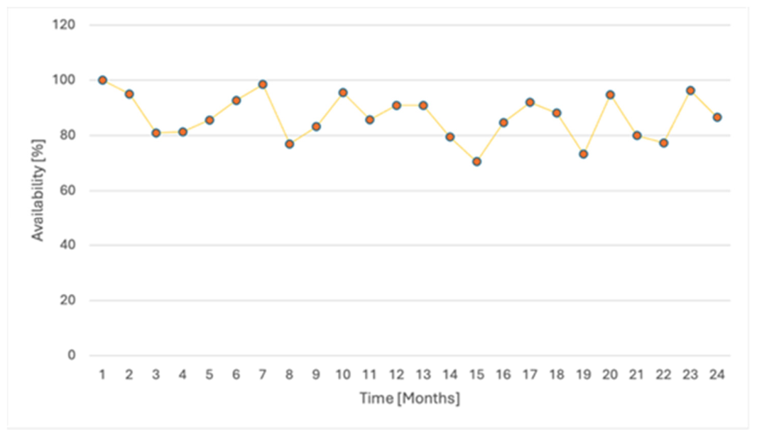
Figure 1 illustrates this temporal dynamic of the system’s availability. Under normal conditions, the system operates at a nominal level; however, when a failure occurs, the system’s functionality and availability experience a deviation, typically observed as a sudden drop. This decline may drive the availability to a lower state, followed by a recovery phase.

Figure 1. Time series representing the temporal dynamic of the system’s availability.

The methodological process involves a structural segmentation of the availability time series. To quantify resilience, we must first identify “Disturbance Events” by detecting local minima (valleys) in the performance curve. The process follows these stages:

(1)

Point Identification: The time series is treated as a set of discrete coordinates, where represents time and availability.

(2)

Peaks and Valleys Detection: Utilizing a peak-detection logic (referred to here as “detecting peaks”), the algorithm identifies significant drops in availability and their consecutive recuperation.

(3)

Vector Construction:

• Period Vectors: These connect successive points of high performance or the onset of a disturbance.
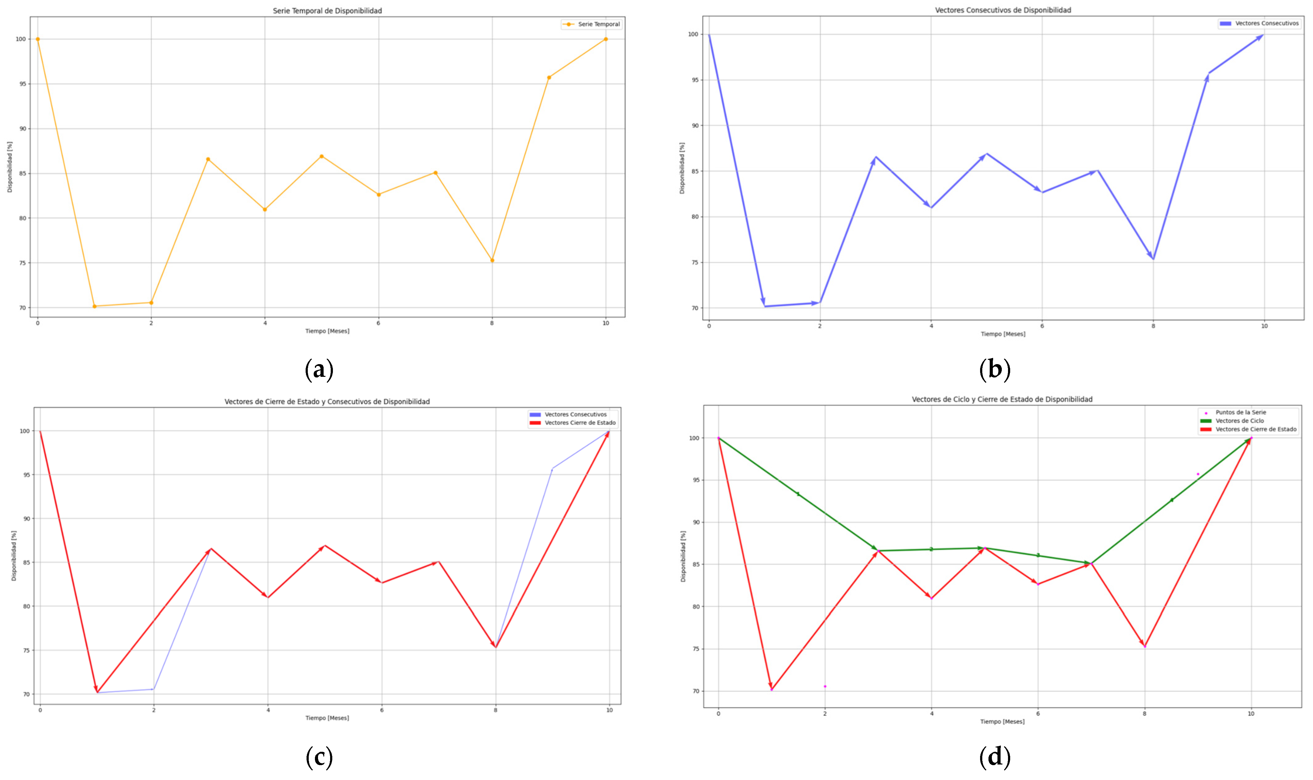
• Cycle Vectors: These group consecutive period vectors sharing a common direction, encapsulating the overall system response to a perturbation from the onset of deterioration through full recovery (formally defined in Section 4.2 and depicted in Figure 2).
• Closure Vectors: These represent the recovery phase, connecting the point of maximum disturbance (the valley) back to the subsequent recovery point (formally defined in Section 4.3 and depicted in Figure 2).

Figure 2. Vectorization process, step by step. (a) Original time series. (b) Vectorized time series. (c) Cycle vectorized. (d) Closure vectors.

(4)

Triangulation: The aforementioned vectors constitute the three sides of the triangles. Then, using Heron’s formula, the areas that represent the resilience loss during each specific event are obtained.

The following subsections provide a detailed description of the phases mentioned above.

4.1. Vector Transformation

In the analysis of critical assets or critical systems’ resilience, availability is a determinant factor. The starting point is a time series of raw data ${\left({\mathrm{t}}_{\mathrm{i}},{\mathrm{A}}_{\mathrm{i}}\right)}_{\mathrm{i}=1}^{\mathrm{n}}$. Each pair $({\mathrm{t}}_{\mathrm{i}},{\mathrm{A}}_{\mathrm{i}})$ provides a point-in-time snapshot of the system’s state of availability. Where the involved variables are identified as:

• i: identifier suffix for point in time.
• n: number of raw data.

The objective of the vector transformation is to convert the sequence of points into a geometric representation that simultaneously captures the magnitude and direction of the changes between adjacent values, thereby facilitating the interpretation of the dynamics of the availability behavior.

The application of vector transformation to availability time series offers advantages over traditional aggregate metrics. By treating each availability increment or decrement as a geometric vector with specific magnitude and orientation, the proposed methodology preserves the informational richness of each sampling instant. The vector-based approach is characterized by four fundamental qualities:

• Preservation of Temporal Dynamics: The transformation generates vector variations directly from the original data without requiring modification. This allows for a detailed analysis of all transitions experienced by the asset, maintaining the sequence and intensity of events.
• Geometric Interpretability: The intrinsic properties of a vector—magnitude (representing the intensity of change) and angle (representing the direction of the process)—provide intuitive metrics for engineering decision-making. Geometrically, an upward inclination (0° < θ < 90°) communicates recovery, while a steep downward slope (270° < θ < 360°) indicates degradation. This interpretability facilitates the communication of diagnostics without requiring advanced statistical training.
• Cycle Modeling: Real-world industrial systems rarely experience a single shock followed by a single recovery; they frequently undergo multiple events. The vector approach, proposed here, allows for the delimitation and quantification of each deterioration-recovery cycle independently. This capability enables direct comparisons between different cycles and a detailed analysis of the evolution of resilience over time.
• Scale Flexibility: Changing the temporal resolution (e.g., from daily to monthly granularity, for instance) does not require the recalibration of the metrics. It is sufficient to redefine the sampling step to generate new vectors, ensuring comparability between systems with different data cadences.

4.2. Cycle Vectors

As it was mentioned, two consecutive points (Figure 2a) are transformed into vectors ($\overrightarrow{{\mathrm{v}}_{\mathrm{i}}}$) providing three essential descriptors that characterize the local dynamics of the series (Figure 2b):

Magnitude: Consider the following two relations:

$$\Delta A=A_{i+1}-A_i,$$

(1)

$$\Delta t=t_{i+1}-t_i$$

(2)

The Euclidean norm quantifies the intensity or ‘size’ of the availability change between two consecutive instants. Calculated via the Euclidean norm (Equation (3)) a high value of $\overrightarrow{v_i}$ reveals a slow process of drop and recovery, whereas low magnitudes indicate short disruptions effects.

$$‖{\overrightarrow{v}}_i‖=\sqrt{{\left({\Delta t}_i\right)}^2+{\left({\Delta A}_i\right)}^2}$$

(3)

Sense: In this approach, the ‘sense’ of all vectors is strictly from left to right, given that the temporal coordinate t advances irreversibly towards the future. That is, each vector $\overrightarrow{v_i}$ connects a preceding instant (t_i, A_i) with a subsequent one (t_i+1, A_i+1); consequently, its horizontal component Δt is always positive, and the vector points to the right. This value remains constant for a given vector, reflecting the interval between consecutive data points, where the context is defined by the unit of time measurement employed. This eliminates ambiguities: time does not regress, and there is no need to classify vectors by a vertical ‘sense’ of progression.

Direction: The direction of $\overrightarrow{v_i}$ describes the inclination of the displacement within the time-availability plane and is expressed via the angle θ of the vector $\overrightarrow{{\mathrm{v}}_{\mathrm{i}}}$ that connects a preceding instant (t_i, A_i) with a subsequent one (t_i+1, A_i+1), concentrated within quadrants I and IV. Values between 1° and 90° indicate increases in availability compared to the availability value prior to the perturbation instant, while those between 0° and −90° signal decreases. Angles of 0° and 360° indicate availability stability.

This unified treatment simplifies the analysis and ensures that all vectors reflect the system’s temporal availability progression without exception. Consequently, the behavior of the asset in question is understood primarily through direction (positive or negative slope) and magnitude.

Consecutive vectors that share a common direction are grouped to form the Cycle Vector ($\overrightarrow{w}$). Subsequently, the Cycle Vector (See Figure 2c, red lines) is defined as the minimum unit that encapsulates the overall system response to a perturbation, grouping the entire trajectory from the onset of deterioration to the beginning of recovery and from the beginning of recovery to full recovery (stabilization or a new decline in availability). This means that each perturbation in availability behavior will have two cycle vectors associated with one of three possible states.

A state is defined as a grouping of vectors that share a common direction, determined by their inclination relative to the temporal axis. This inclination is calculated via the vector angle, allowing for classification into three primary states:

• Deterioration: Vectors with negative inclination, signaling a drop in availability.
• Stability: Horizontal vectors, reflecting constant availability.
• Recovery: Vectors with positive inclination, indicating an increase in availability.

The categorization of states depends directly on the vector’s inclination; thus, the angle formed with respect to the time axis is determinant for this classification. Table 2 presents the angular ranges corresponding to each defined state.

Table 2. States According to Angle.

State	Angle
Recovery	0° < θ < 90°
Deterioration	270° < θ < 360°
Stability	θ = 0°; θ = 360°

Note that vectors within the angular range > 90° to <270° are not possible. Values in this range would imply displacement solely along the vertical axis (y-axis) or a backward displacement along the temporal axis, which is impossible given that the horizontal axis represents the passage of time.

This classification transforms the sequence of vectors into a chain of states (deterioration, stability, recovery), simplifying the understanding of system evolution and allowing analysis to focus on critical moments of change. Conversely, a recovery state is associated with the fact that performed maintenance actions begin to consolidate, causing an increase in the availability indicator.

4.3. Closure Vectors

Once the series of states has been established and considering that each disruptive event affecting system availability can be represented by at least one deterioration vector and one recovery vector, a new vector is generated that connects the onset of the deterioration state with the end of the recovery state. This vector is referred to as the closure vector (Figure 2d, green vectors).

The procedure of obtention of each closure vector is represented in Equation (4). The resulting vector concentrates the accumulated change in the entire phase in its magnitude, the predominant trend (ascending in recoveries or descending in drops) in its angle, and the total state duration in its temporal component.

$${\overrightarrow{w}}_{closurej}=\sum _{i=1}^n\overrightarrow{v_i}=\left(\sum _{i=1}^n\Delta t_i,\sum _{i=1}^n\Delta d_i\right)$$

(4)

where the involved variables are identified as:

• j: Identifier suffix for the state closure vector.
• n: Number of consecutive vectors within a state.

The following pseudo-code (Algorithm 1) outlines the logic for identifying these events and constructing the associated vectors using a peak-detection approach.

Algorithm 1 Vectorization of Availability Time Series for Resilience Calculation

1: Input: Time series $T=\{\left(t_0,A_0\right),\left(t_1,A_1\right),\dots ,\left(t_n,A_n\right)\}$ 2: Output: Set of geometric triangles $\mathcal{T}=\{{\Delta }_1,{\Delta }_2,\dots ,{\Delta }_k\}$ 3: 4: procedure ExtractVectors($T$) 5:        $\widehat{A}\leftarrow 100-T.A$ ▷ Invert series to treat drops as peaks 6:        $V\leftarrow \mathrm{detect}\_\mathrm{peaks}\left(\widehat{A},\mathrm{mpd}=1,\mathrm{mph}=5\right)$    ▷ Identify indices of maximum disruption 7:        for each index $i\in V$ do 8:                $P_{\mathrm{start}}\leftarrow \left(t_{i-1},A_{i-1}\right)$    ▷ Pre-event baseline 9:                $P_{\mathrm{m}\mathrm{i}\mathrm{n}}\leftarrow \left(t_i,A_i\right)$    ▷ Vertex of maximum perturbation 10:                $P_{\mathrm{end}}\leftarrow \left(t_{i+1},A_{i+1}\right)$    ▷ Recovery point 11:                Vector Definition: 12:                ${\overrightarrow{v}}_{\mathrm{period}}\leftarrow P_{\mathrm{m}\mathrm{i}\mathrm{n}}-P_{\mathrm{start}}$    ▷ Downward vector (Green) 13:                ${\overrightarrow{v}}_{\mathrm{closure}}\leftarrow P_{\mathrm{end}}-P_{\mathrm{m}\mathrm{i}\mathrm{n}}$    ▷ Recovery vector (Red) 14:                Euclidean Side Lengths: 15:                $a\leftarrow ∥{\overrightarrow{v}}_{\mathrm{period}}∥$ 16:                $b\leftarrow ∥{\overrightarrow{v}}_{\mathrm{closure}}∥$ 17:                $c\leftarrow ∥P_{\mathrm{end}}-P_{\mathrm{start}}∥$ 18:                $\theta \leftarrow \mathrm{atan}2\left({\overrightarrow{v}}_{\mathrm{closure}}.y,\hspace{0.25em}{\overrightarrow{v}}_{\mathrm{closure}}.x\right)$    ▷ Calculate closure angle 19:                ${\Delta }_i\leftarrow \left(a,b,c,\theta \right)$ 20:                add ${\Delta }_i$ to $\mathcal{T}$ 21:        end for 22:        return $\mathcal{T}$ 23: end procedure

The angle θ of the closure vector with respect to the horizontal axis is a critical indicator that can represent the quality of recovery and, therefore, the degree of the asset or system of asset resilience. This angle varies within the range [−90°, 90°]. When the angle is negative, it means that the availability achieved through the recovery process is lower than the availability level prior to the disruptive event. Conversely, when the angle is positive, it indicates that the availability reached as a result of the recovery process exceeds its initial value before the shock. Therefore, the goal is θ → 90°, which would indicate a rapid and significant recovery.

The closure vector representation is an intentional modeling simplification: the recovery trajectory between the disruption onset and the recovery endpoint is abstracted as a straight line, characterized entirely by its magnitude and inclination angle θ. As a consequence, two disruption events sharing identical start and end points but differing in their intermediate recovery dynamics—for instance, a convex profile in which most of the recovery occurs early, versus a concave profile in which recovery accelerates only near the end—yield identical closure vectors and therefore identical values of Fa and ρ. The indicator captures end-state recovery fidelity but does not distinguish trajectory shape. This simplification is considered appropriate for the industrial context addressed in this work for two reasons. First, availability data from production systems are measured at discrete intervals and subject to operational noise, superimposed maintenance events, and Monte Carlo sampling variability. Under these conditions, the intermediate trajectory between disruption and recovery is not a smooth analytical curve but a noisy signal around a central tendency; the closure vector provides a robust estimate of that tendency, less sensitive to measurement noise than any metric attempting to follow the exact intermediate path. Second, from a maintenance management perspective, the operationally relevant question is how much availability was lost and how quickly the system returned to its nominal level—not the precise shape of the path between those two states. The closure vector answers that question directly.

Future extensions of the framework could replace the straight-line closure vector with a parametric curve fit—such as a logistic or Gompertz function—or employ line integrals over the actual recovery path to capture trajectory-dependent recovery dynamics. A complementary shape index, defined as the ratio of the actual recovery area to the triangular area, could also be introduced as a secondary descriptor without modifying the core geometric formulation.

4.4. Impact Triangle and ρ Definition

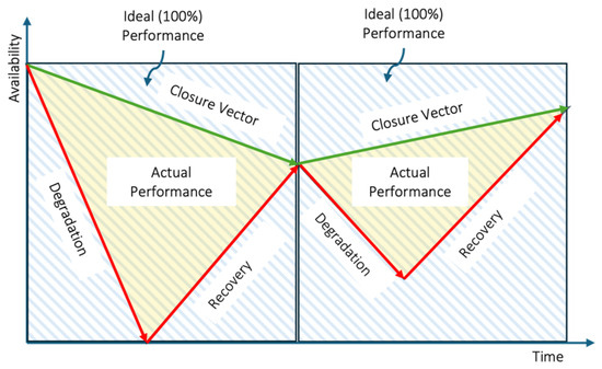
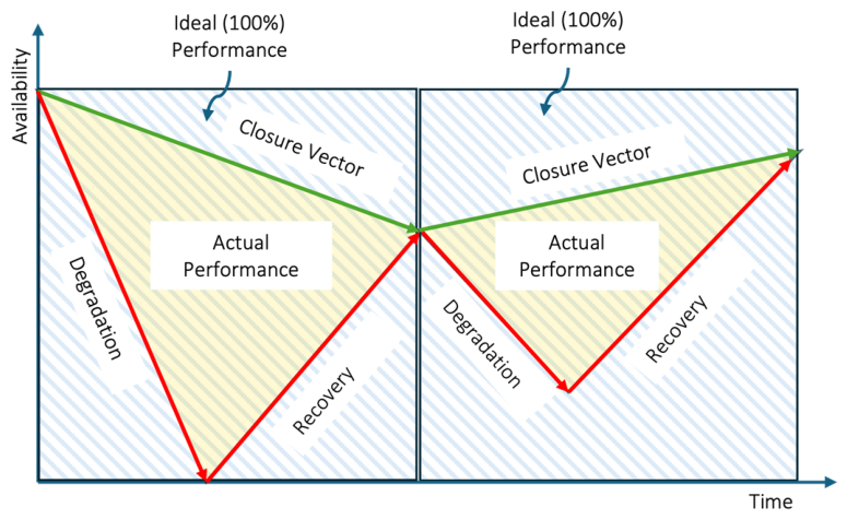
Once all Cycle Vectors (indicated in red) and Closure Vectors (indicated in green) have been defined across the time series, they collectively establish a sequence of closed geometric shapes. Specifically, these intersections define a series of triangles spanning the duration of the study. Within this framework, each individual vector is no longer viewed merely as a directional displacement but is instead treated as a formal side of a triangle. Each segment of the cycle and its corresponding closure vector form the boundaries of these shapes. It is important to note that since the Theta angles ($\theta$) of each identified triangle are non-zero, the resulting figures are characterized as inclined triangles.

The proposed resilience metric is based on the fundamental principle of analyzing triangular areas derived from the vector transformation of the availability time series. Therefore, these areas make it possible to calculate the proportion between the area of each triangle representing the loss of availability and the area of the region associated with a theoretical situation without damage due to disruptive events. This approach has the following advantages:

• The projections of the closure vector correspond to the recovery time in response to the disruptive event.
• It is applicable to systems regardless of whether their performance can be fully restored within the time considered as recovery time.

Once these triangles have been geometrically defined by the cycle and closure vectors, their specific properties can be quantified. To determine the magnitude of the impact or performance within each segment, the area of each triangle is calculated using Heron’s Formula. By utilizing the lengths of the three vectors that constitute the sides of the triangle (a, b, c), the semi-perimeter (s) is first established:

$$s={\displaystyle \frac{a+b+c}{2}}$$

(5)

Then, the triangle area (A) is computed as the square root of the product of the semi-perimeter and its differences with each side, expressed as:

$$A=\sqrt{s\left(s-a\right)\left(s-b\right)\left(s-c\right)}$$

(6)

The proposed metric, based on the vectorial approach, enables a geometric analysis focusing on the impact, duration, and trend of each cycle. These three elements are implicit in the triangle area which is fundamental for quantifying the resilience indicator.

The resilience for a specific event or cycle is calculated as the product of two dimensionless factors derived from geometric analysis: a normalized area ratio that quantifies the extent and depth of the availability loss relative to the most severe event in the series, and an angle-based weighting factor derived from the inclination of the closure vector, which penalizes incomplete or slow recoveries while rewarding rapid restoration beyond the pre-shock baseline. To quantify the performance and resilience of the system, this study introduces a resilience indicator, ${\rho }_i$, which is based in a vectorial approach. The indicator is defined by the following expression:

$${\rho }_i={\displaystyle \frac{A_i^{dmg}}{max\left(A_i^{dmg}\right)}}\cdot \left({\displaystyle \frac{1-\mathit{sin}\theta }{2}}\right)$$

(7)

where ${\mathrm{A}}_i^{dmg}$ represents the evaluated area of the damage triangle and $max\left({\mathrm{A}}_i^{dmg}\right)$ denotes the maximum area of the damage triangle among all the triangles along the entire period under analysis (see Figure 3). Normalizing by max() ties the indicator’s scale to the most severe event within the analyzed period, making ρ_i suitable for intra-system, intra-period comparison—which is the primary objective of the present study. This normalization strategy has two known limitations. First, if the same system is analyzed across different time windows and the maximum damage event differs between windows, ρ values are not directly comparable across periods; for longitudinal benchmarking, max(Aᵈᵐᵍ) should be fixed to a reference value established during an initial calibration period. Second, if two different systems are compared and their respective maximum damage events differ in magnitude, their ρ values are normalized against different references; a value of ρ = 0.4 in system A does not imply the same absolute resilience loss as ρ = 0.4 in system B. Users intending cross-system benchmarking should adopt one of the alternative normalization strategies discussed in Section 7. The term $\left({\displaystyle \frac{1-\mathit{sin}\theta }{2}}\right)$ serves as the Angle Factor, a dimensionless weighting component that penalizes incomplete or slow recoveries based on the inclination of the closure vector. The sine function was selected because sin θ directly represents the vertical component of the unit closure vector in the time-availability plane, providing a geometrically grounded measure of recovery magnitude relative to recovery duration. No additional calibration parameter is introduced, and the function possesses four desirable mathematical properties. First, continuity: sin θ is continuous on ℝ, so Fa is continuous on [−90°, 90°] with no discontinuities or artificial thresholds. Second, strict monotonicity: the derivative dFa/dθ = −cos θ/2 is strictly negative on the open interval (−90°, 90°), meaning that a higher closure vector angle—corresponding to faster and more complete recovery—always produces a lower penalty, without exception. Third, normalization: Fa (90°) = 0 and Fa (−90°) = 1, so the factor maps exactly onto [0, 1] without requiring any post hoc rescaling. Fourth, maximum sensitivity at θ = 0°: since |dFa/dθ| = cos θ/2 is maximized at θ = 0°, the factor is most discriminating precisely in the range of intermediate recovery trajectories, where differentiation between system configurations is most operationally relevant.

Figure 3. Impact triangle concept.

The resilience indicator ${\rho }_i$ is formulated as a damage-based metric, analogous to the resilience loss function of Bruneau et al. [7]. Consequently, higher values of ${\rho }_i$ indicate greater resilience loss (a more severe or poorly recovered disturbance event), while lower values indicate better system resilience. A value of ${\rho }_i=0$ would correspond to an idealized instantaneous recovery that fully restores or exceeds the pre-shock availability level.

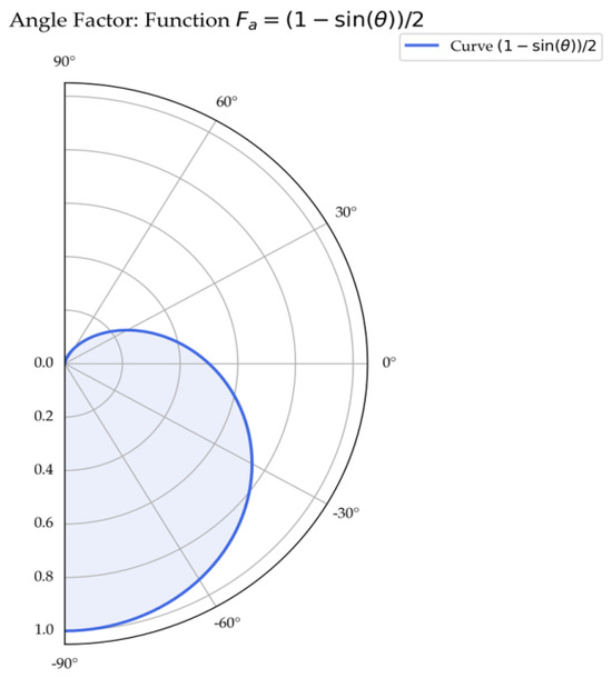
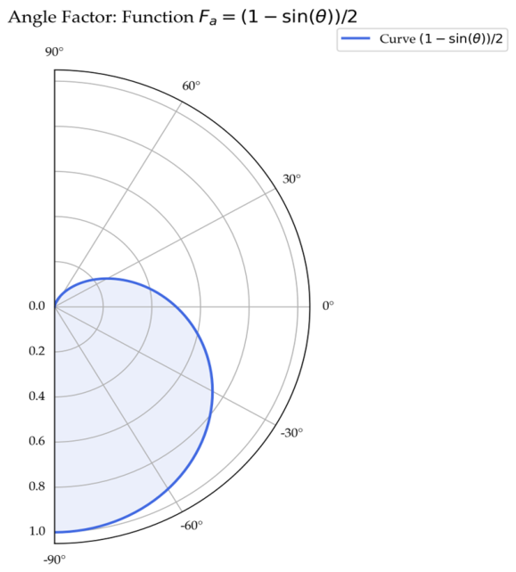
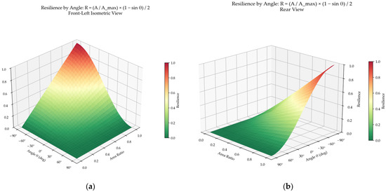
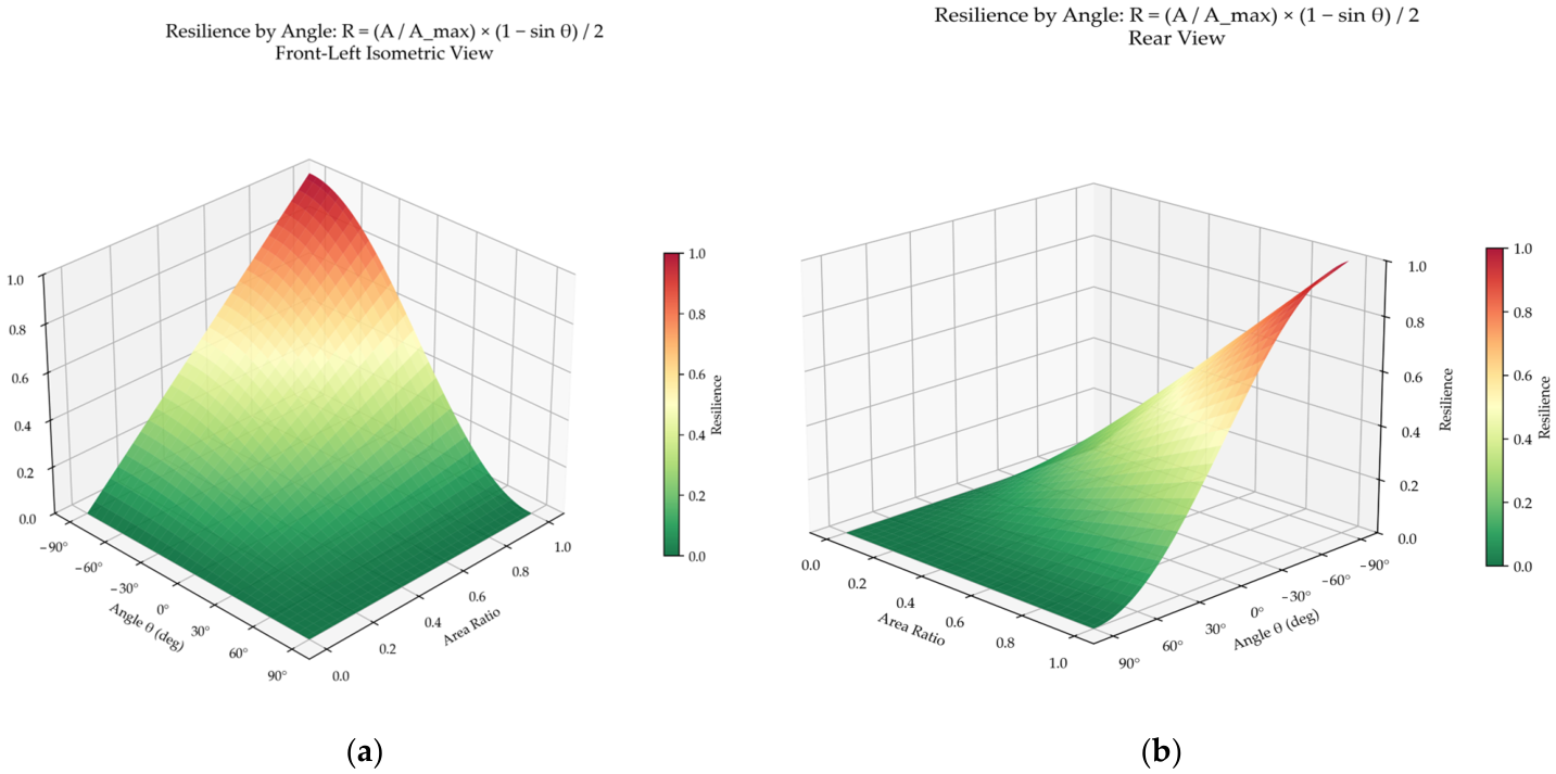
The behavior of the weighting component within the resilience indicator is illustrated in Figure 4. This polar plot maps the response of the Angle Factor, Fa, across an angular range from 90° to −90°. As observed, the function exhibits a non-linear monotonic increase as the angle $\theta$ transitions from positive to negative values. Specifically, at the zenith ($\theta =90°$), the factor nullifies, representing an idealized structural state. The neutral condition ($\theta =0°$) yields a factor of 0.5, serving as the baseline for standard configurations. Conversely, as the angle reaches −90°, the factor attains its maximum value of 1.0, which maximizes the magnitude of the resilience coefficient $\rho$, thereby indicating a critically degraded state. This visual representation confirms that the proposed trigonometric weighting effectively penalizes negative structural configurations while rewarding positive geometric orientations. Figure 5 presents a comprehensive 3D surface plot visualizing the relationship between the resilience index, (plotted on the Z-axis), and its two defining components: the Area Ratio and the $\theta$. This isometric view provides a clear perspective on the indicator’s behavioral domain with a color gradient, ranging from green, representing favorable high-resilience conditions, to red, signifying critical low-resilience states. The response surface reveals that the Area Ratio scales the overall magnitude of the indicator, while the angle factor governs the shape of the decay curve.

Figure 4. Closure vector impact, graphic representation.

Figure 5. Surface plot of the relationship between the resilience index and its two defining components: the Area Ratio and the $\theta$ angle. (a) Front-Left Isometric view. (b) Rear View.

Analyzing the surface graphs, one can observe that the Resilience indicator is maximized at an Area Ratio close to 1.0 and with steep negative fall angles, signifying high-velocity recovery. In addition, a systematic decline in resilience as the angle approaches 90°, marking the threshold where the system possesses zero reactive capacity against the perturbation.

The proposed methodology allows for the dynamic evaluation of resilience throughout the operational life of an asset. As illustrated in Figure 3, the availability time series is characterized by a sequence of “period vectors” (red) and “closure vectors” (green). Each significant disruption in the series forms a distinct geometric unit—a triangle—defined by the deviation between the planned availability and the actual performance recovery.

Individual Event Quantification: For each discrete disruptive event i, an individual resilience coefficient ${\rho }_{\mathrm{i}}$ is calculated (by applying Equation (7)). This value serves as a specific indicator of the system’s response to a specific perturbation at time t. This allows for the identification of specific events where the system exhibited either high vulnerability (high ${\rho }_i$) or robust recovery (low ${\rho }_i$).

Aggregate Resilience for Longitudinal Analysis: While ${\rho }_i$ provides insights into isolated incidents, industrial asset management often requires a single, representative metric to benchmark the overall performance of a system over a sustained period (e.g., a fiscal year or a complete maintenance cycle). In such cases, where the time series includes multiple disruptive events, the global resilience indicator ($\overline{\rho }$) is determined by the arithmetic mean of all individual coefficients calculated for the series:

$$\overline{\rho }={\displaystyle \frac{1}{n}}\sum _{i=1}^n{\rho }_i$$

(8)

where n is the total number of identified triangles within the analyzed timeframe. This aggregate value $\overline{\rho }$ provides a stabilized metric that smooths out stochastic variations, allowing for a high-level comparison between different systems or the tracking of the same system’s degradation over several years.

The computational algorithm for quantifying system resilience is formalized in Algorithm 2. This procedure executes the transition from raw geometric data and triangular representation—derived from the availability time series—into a normalized, longitudinal indicator suitable for asset management benchmarking.

Disruption events are identified automatically from the structure of the availability time series, without requiring user-defined threshold parameters. The algorithm detects local minima—points where availability reaches a value lower than all neighboring observations—followed by the nearest local maximum representing the recovery peak. Each minimum-maximum pair defines one disruption-recovery cycle. The depth of the local minimum relative to the pre-disruption level and the temporal distance to the recovery peak are computed descriptors of each detected event, derived entirely from the data. This procedure is self-calibrating and requires no domain-specific parameter tuning, making it directly applicable to availability series from different industrial contexts without modification. This approach facilitates the transition from event-based analysis to a longitudinal management perspective, enabling the benchmarking of different assets or the evaluation of a single system’s resilience evolution throughout its lifecycle. The following section analyses the indicator’s typical behavior across various post-shock system responses.

Algorithm 2 Calculation of the Resilience Indicator ($\rho$)

1: Input: Set of Triangles $\mathcal{T}=\{{\Delta }_1,{\Delta }_2,\dots ,{\Delta }_k\}$, Maximum Area $A_{max}$ 2: Output: Resilience coefficients$\{{\rho }_1,{\rho }_2,\dots ,{\rho }_k\}$ and Global Mean $\bar{\rho }$ 3: 4: procedure ComputeResilience ($\mathcal{T},\hspace{0.25em}{A}_{max}$) 5:        $Total\_Rho\leftarrow 0$ 6:        $n\leftarrow count\left(\mathcal{T}\right)$ 7:        for each ${\Delta }_i=\left(a,b,c,\theta \right)$ in $\mathcal{T}$ do 8:                1. Calculate Semi-perimeter ($s$): 9:                $s\leftarrow \left(a+b+c\right)/2$ 10:                2. Calculate Evaluated Area ($A_{ev}$) via Heron’s Formula: 11:                $A_{ev}\leftarrow \sqrt{s\left(s-a\right)\left(s-b\right)\left(s-c\right)}$ 12:                3. Determine Weighting Factor ($W$): 13:                $W\leftarrow \left(1-sin\theta \right)/2$ 14:                4. Compute Individual Resilience (${\rho }_i$): 15:                ${\rho }_i\leftarrow \left(A_{ev}/A_{max}\right)\cdot W$ 16:                $Total\_Rho\leftarrow Total\_Rho+{\rho }_i$ 17:                Save ${\rho }_i$ 18:        end for 19:        5. Calculate Global Longitudinal Resilience ($\bar{\rho }$): 20:        $\bar{\rho }\leftarrow Total\_Rho/n$ 21:        return $\left\{{\rho }_i\right\},\hspace{0.25em}\bar{\rho }$ 22: end procedure

4.5. Base Case Study: Assessing the Sensitivity of ${\rho }_i$

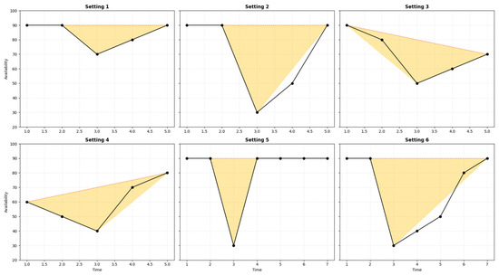
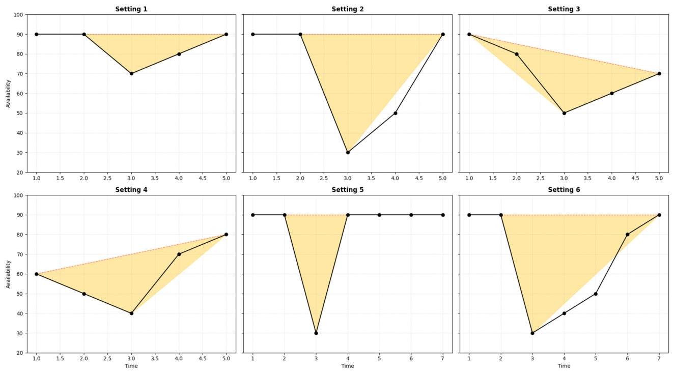
In this initial phase, the behavior of the resilience metric was evaluated against controlled variations in the geometry of availability loss events. Six distinct scenarios (Settings) were considered to observe how the ‘shape’ of the failure effects—and the resulting availability behavior—impacted the final resilience indicator. Figure 6 illustrates the availability patterns in response to a failure event. Table 3 displays the resilience indicator values calculated for each respective case.

Figure 6. Availability patterns addressed by the sensitivity study.

Table 3. Resilience indicator values calculated for each respective setting.

Setting	Event Description	Resilience ($\mathit{\rho }$)
Setting 1	Moderate drop (90% to 70%) with a rapid 4-period recovery.	0.150
Setting 2	Abrupt drop (90% to 30%) with the same rapid recovery time.	0.450
Setting 3	Abrupt drop (90% to 50%) followed by an incomplete recovery stabilizing at 70%.	0.594
Setting 4	Moderate disruption where the system improves to 80% availability from a 60% baseline.	0.006
Setting 5	Deep drop to 30% availability with an exceptionally fast, complete recovery.	0.300
Setting 6	Same depth as Setting 5, but with a more gradual recovery, increasing the event area.	0.750

Lower ρ = better resilience; higher ρ = greater resilience loss.

The six experimental settings provide a granular look at how the proposed resilience indicator ($\rho$) responds to diverse disruptive geometries. By keeping the recovery time constant in several scenarios while varying the depth and stability of the recovery, the metric demonstrates a sophisticated ability to prioritize the “quality” of system restoration over mere survival. The contrast between Settings 1, 2, and 3 highlights the metric’s sensitivity to the final state of the system post-shock:

• Recovery to Baseline: In Setting 1 and 2, despite significantly different drop depths (70% vs. 30% availability), both systems return exactly to their original 90% state. The resulting $\rho$ values (0.150 and 0.450) reflect that the indicator effectively weights the area of lost availability while acknowledging the successful return to a 0° angle.
• System Degradation: Setting 3 presents a critical case where the system fails to reach its pre-shock level, stabilizing at 70% instead of 90%. The negative recovery angle ($\theta$ < 0°) acts as a penalty, reflecting a loss of long-term system integrity despite a seemingly higher $\rho$ (0.594) compared to the deep drop of Setting 2.

Setting 4 offers the most distinct result, where a system initially at 60% availability recovers to a superior 80% state.

• Positive Angular Influence: This scenario results in a recovery angle greater than 0°, which the model interprets as a beneficial adaptation.
• Critical Resilience Threshold: Interestingly, this setting yielded the lowest numerical $\rho$ (0.006). This suggests that while the “quality” of recovery was high (positive angle), the prolonged duration spent at the 40% nadir during the event created an “event area” so substantial that the system’s immediate resilience was nearly compromised.

The comparison between Settings 5 and 6 isolated the variable of recovery speed following identical deep drops to 30%:

• Exceptional Velocity: Setting 5 features an “exceptionally fast” recovery, resulting in a $\rho$ of 0.300. The minimized duration of the disruption is key here, as the system spends very little time in a failed state.
• Gradual Recovery Penalization: Setting 6, with its gradual recovery, produced a much larger event area. Consequently, its resilience score rose to 0.750. This demonstrates that the indicator is highly sensitive to the integral of lost availability over time; the longer a system lingers in a sub-optimal state, the more its resilience indicator is negatively impacted, regardless of achieving a full final recovery.

These six cases confirm that the proposed indicator is not a static measurement of failure depth. Instead, it is a dynamic assessment of absorptive capacity (how much availability is lost) and restorative quality (the angle and speed of the return). The results validate that the most resilient systems are those that minimize the area of disruption and, where possible, leverage the recovery phase to improve the system’s baseline state. In the next section, a case study using actual operational data is presented to illustrate the performance and applicability of the indicator regarding modifications in the configuration of a production system.

5. Case Study: A Comminution Plant

5.1. Milling Area Description

This case study is based on a real mining operation located in northern Chile, specifically focusing on the comminution circuit of a sulfide copper concentrator. The analysis is focused on the milling stage, a critical process for maximizing recovery in subsequent flotation stages. The operational sequence begins with primary crushing and feeding into the Semi-Autogenous Grinding (SAG) mill. The discharge from the SAG mill is then screened; the oversize fraction (pebbles) is recirculated, while the undersize fraction forms a slurry that must be transported under specific hydraulic conditions.

Historically, this specific plant has faced a bottleneck in its milling lines. Operational data indicates that ball mills underperform compared to SAG mills, primarily due to the high failure rate of the hydrocyclone feed pumps. These pumps are critical for maintaining the correct pressure and density in the classification stage; any failure here results in an immediate loss of system availability.

5.2. System Architecture and Modeling

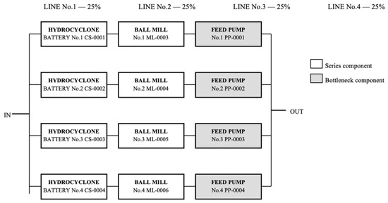
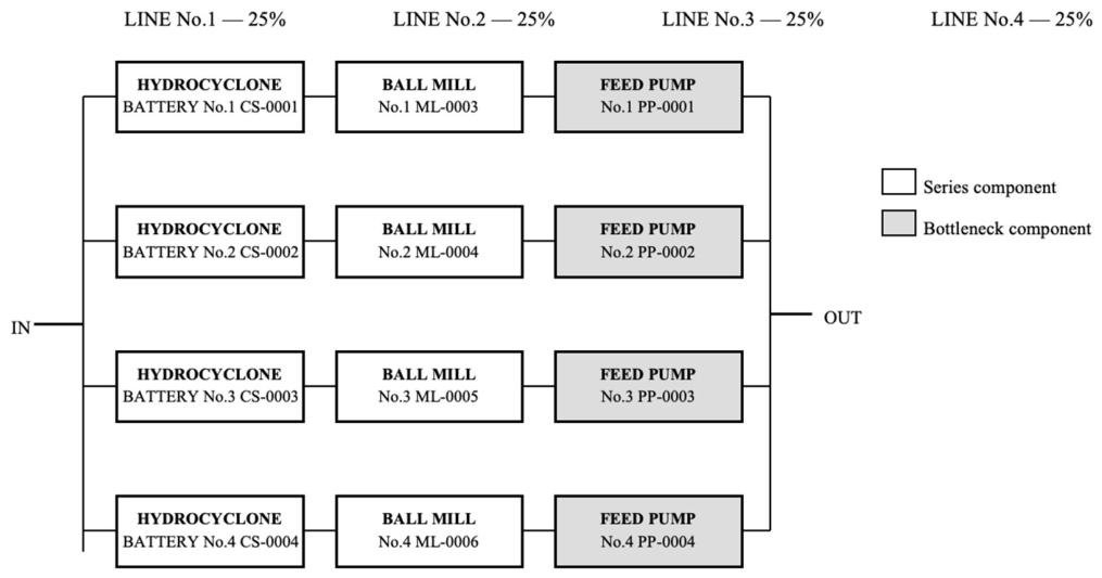
The actual system consists of four independent processing lines, each designed to handle 25% of the total throughput.

To model the system’s logic, each line was represented through a series of functional blocks (RBD). Each asset is identified by a standardized alphanumeric TAG (Figure 7):

Figure 7. Original system configuration.

• ML-01 to ML-04: Ball Mills.
• PP-01 to PP-04: Hydrocyclone Feed Pumps.
• CS-01 to CS-04: Hydrocyclone Batteries.

Reliability, Availability and Maintainability (RAM) parameters were derived from historical plant logs [21,22,23]. The following distributions were utilized for the Monte Carlo simulation:

• Failure behavior: Modeled using Weibull distributions for all components, capturing both infant mortality and wear-out phases.
• Repair Behavior: Modeled using Lognormal distributions for pumps and cyclones, while ball mills followed a Weibull repair profile due to the complexity of mechanical interventions.

A sensitivity analysis using the Jack-Knife technique was implemented to prioritize interventions and assets. This method plots assets based on their Mean Time to Repair (MTTR) against their total number of failures.

• Zone IV (Chronic/Acute): All feed pumps were located here, indicating a higher-than-average failure frequency.
• Zone II (Acute): The ball mills occupied this quadrant, characterized by fewer failures but significantly high repair times due to the magnitude of the equipment (e.g., liner replacements, motor failures).

Based on the identified bottleneck, the study moved from a single-pump serial configuration to three alternative redundancy-based architectures to enhance resilience:

• Fractional Configuration: Two pumps share the load, each operating at 75% of its nominal capacity to reduce individual wear (Figure 8).

  

  Figure 8. Fractioned system configuration.

  Figure 8. Fractioned system configuration.

  
• Parallel Configuration (Active/Active): Both pumps run simultaneously at full capacity. If one fails, the remaining unit can handle the total line demand, ensuring process continuity (Figure 9).

  

  Figure 9. Parallel system configuration.

  Figure 9. Parallel system configuration.

  
• Standby Configuration: A primary pump operates while a second remains in reserve. The backup only enters the critical path if the primary unit fails or requires maintenance (Figure 10).

  

  Figure 10. Standby system configuration.

  Figure 10. Standby system configuration.

  

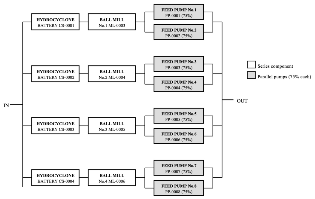
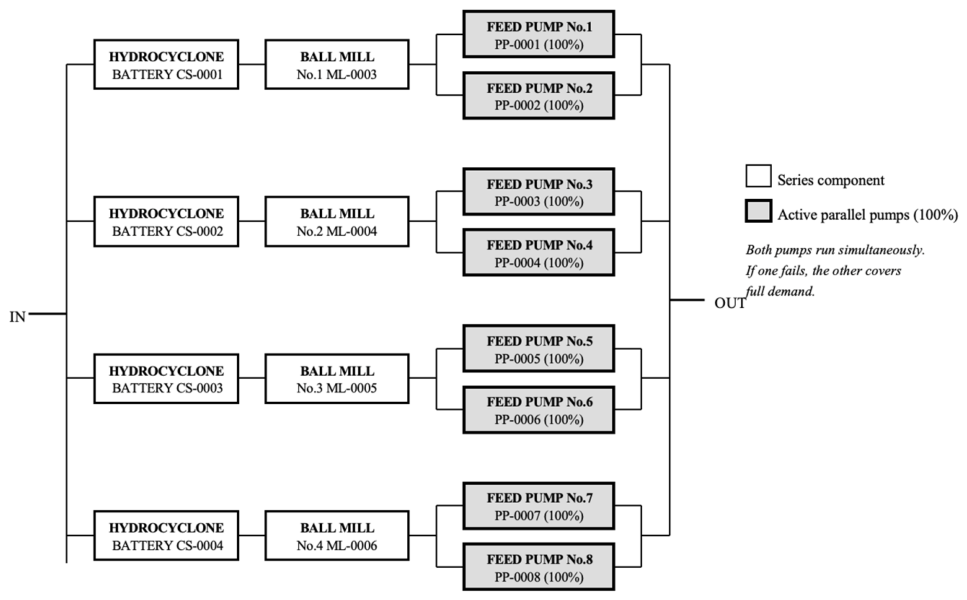
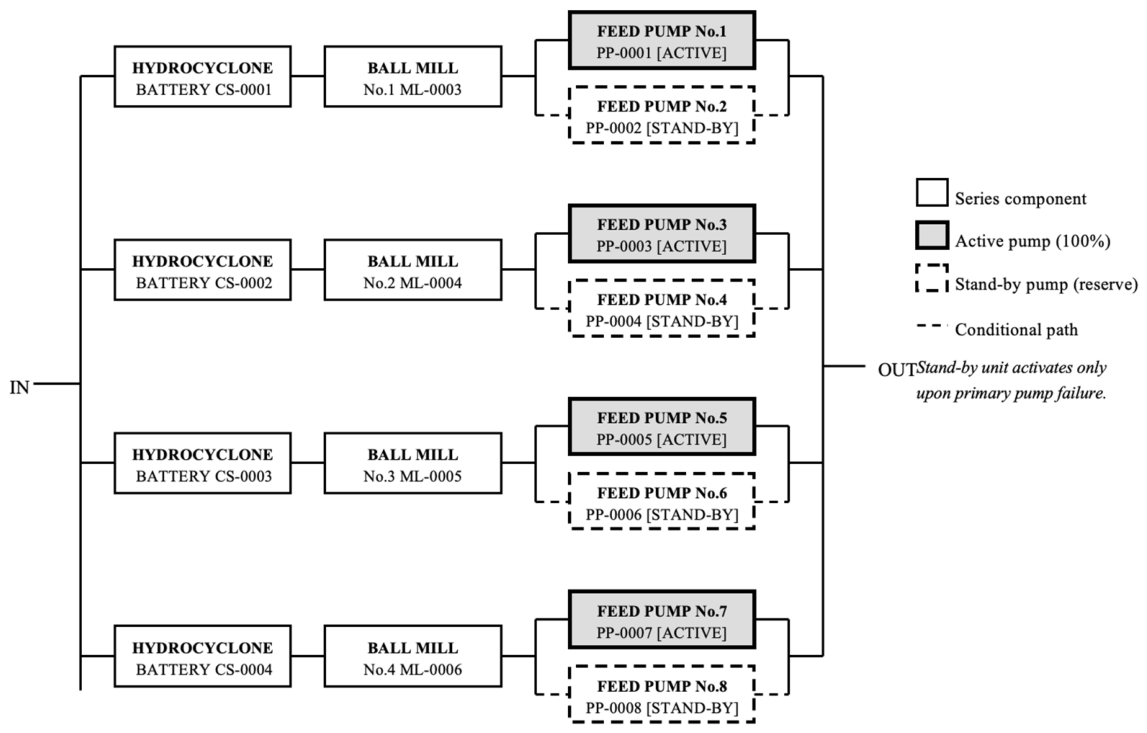
For each scenario, system availability performance was simulated over a 12-month horizon discretized into monthly evaluation intervals. The resilience index was computed per maintenance cycle as the normalized area between the simulated availability curve and an ideal upper bound, capturing both the depth and duration of availability degradation events.

For these hypothetical configurations, maintenance scheduling was structured to optimize resources and maximize operational availability while minimizing process disruption. The addition of a new asset enables the revision and implementation of new maintenance strategies:

5.2.1. Plant Shutdown Strategy (Mills)

The plan focuses on two semi-annual major plant shutdowns dedicated to the four ball mills (ML-01 to ML-04). These shutdowns concentrate technical resources on liner replacements, which define the grinding system’s critical path.

5.2.2. Pumping Line Intervention Logic

A staggered, parallel execution strategy was designed for the feed pumps (PP-01 to PP-04):

• Simultaneous Execution: Two pumping lines are overhauled concurrently to optimize maintenance crews.
• Operational Staggering: A two-month offset is established between the first and second pair of lines, ensuring continuous backup capacity and preventing repair shop saturation.
• Major Shutdown Synchronization: Pump overhauls are scheduled to coincide with mill shutdowns whenever frequency permits, utilizing mill downtime to replace pumps without causing additional production losses.
• Fractional and Parallel Offset: Within the same operating line, fractional and parallel configuration tasks are offset by one week from the primary intervention. This buffer balances the workload and facilitates staggered commissioning tests.
• Standby Units Policy: No scheduled maintenance is planned for standby units due to their minimal mechanical wear from low operation. Maintenance is limited to visual inspections prior to status changes (standby to operational), avoiding unnecessary tasks that do not add system reliability.

5.3. Resilience Quantification

Once the alternative configurations were constructed, using the aforementioned RBDs and reliability and maintainability distributions, along with the adaptation of maintenance plans to these new configurations, RAM [21,22,23] analyses were performed via Monte Carlo experiments [24,25,26], and the series of systemic availability values were obtained for each of these configurations. Using these availability time series, resilience indicators were calculated to analyze which of the proposed configurations would allow the system to gain greater resistance and recovery capacities. Table 4 displays the values of these indicators.

Table 4. Resilience Indicator for each of the alternative configurations.

Settings	Cycle 1	Cycle 2	Cycle 3	Cycle 4	Cycle 5	$\overline{\rho }$
Baseline	0.001	0.184	0.012	0.044	—	0.0603
Fractional 50%	0.079	0.022	0.078	—	—	0.0597
Fractional 70%	0.003	0.086	0.019	0.006	0.062	0.0352
Parallel	0.002	0.129	0.004	0.149	—	0.0710
Standby	0.002	0.217	0.006	0.079	—	0.0760

Lower $\overline{\mathit{\rho }}$ = better resilience.

5.4. Discussion

The resilience indices of Table 4 are interpreted below along three practical dimensions: (1) concentration of resilience loss—whether ρ is dominated by a single event or distributed across cycles; (2) its drivers—depth of availability drop (robustness deficit) versus slowness of recovery (rapidity deficit); and (3) the maintenance action each profile suggests. All configurations fall within the resilient-to-acceptable performance range (ρ < 0.40), confirming that the evaluated topologies represent genuine engineering alternatives rather than clearly inferior choices.

Relevant application domains include manufacturing systems—where the indicator complements OEE metrics with recovery dynamics—power systems, transportation networks, healthcare equipment management, and cyber-physical infrastructures, each characterized by availability time series amenable to the same geometric treatment.

Baseline Configuration

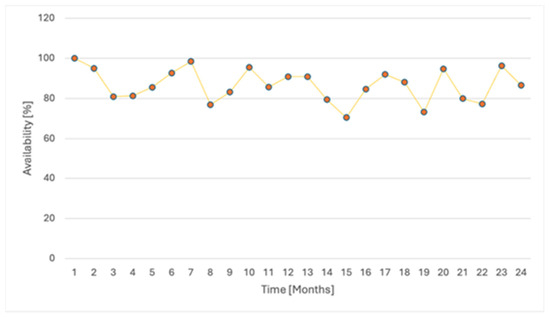
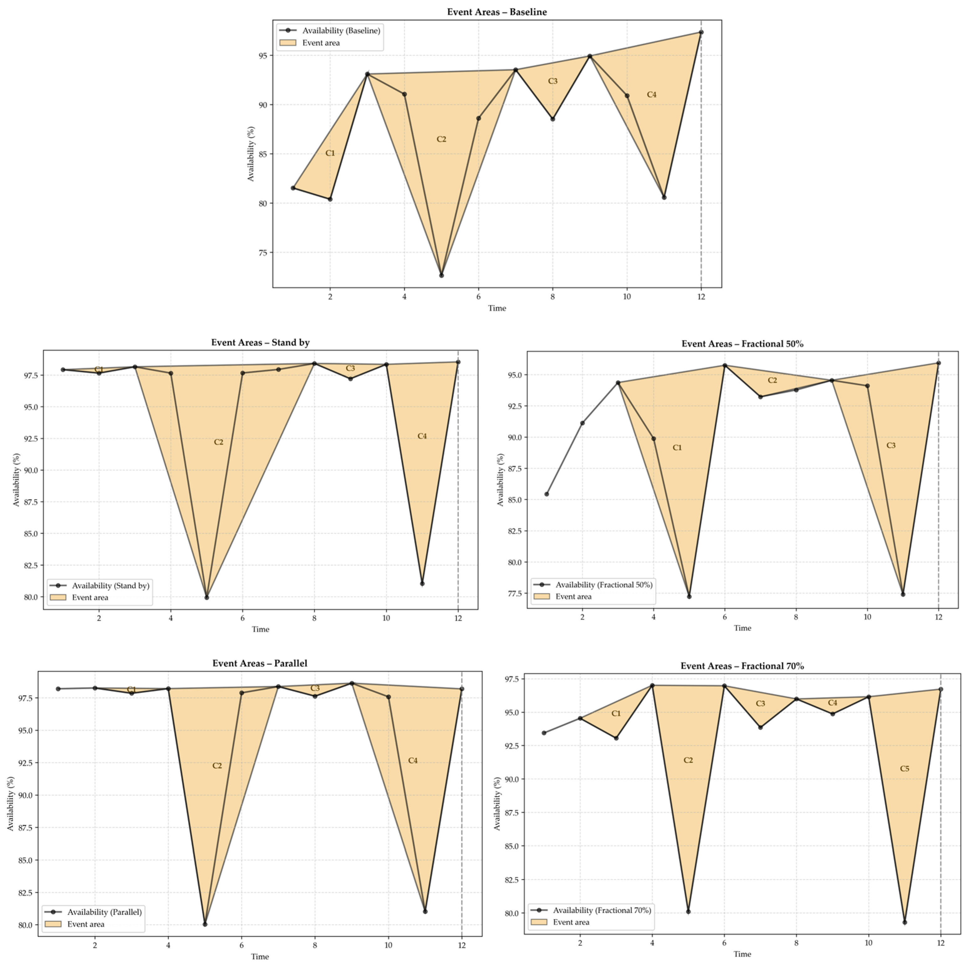
Under the baseline configuration, system availability fluctuates between approximately 72% and 97% across the 12-month simulation horizon (Figure 1). The most pronounced availability drop occurs at month 5, corresponding to the first major planned shutdown of all ball mills. Subsequent recovery is partial, and additional drops are observed at months 8 and 11, aligned with pump preventive maintenance windows. The event areas, represented by the shaded regions in Figure 11, highlight the cumulative availability loss attributable to each maintenance cycle.

Figure 11. Availability behavior for alternative scenarios.

The resilience analysis for the baseline scenario identifies Cycle 2 as the most impactful maintenance event, yielding a resilience index of 0.184 (Figure 11). Cycles 1, 3, and 4 exhibit substantially lower indices (0.001, 0.012, and 0.044, respectively), indicating that the first major plant shutdown concentrates the bulk of productive loss for this configuration.

The concentration of resilience loss in Cycle 2 identifies the simultaneous ball mill shutdown as the dominant vulnerability. Improvement efforts should target the recovery time of that specific event—through spare parts pre-positioning or phased restart sequencing—rather than the overall failure rate.

Fractional 50% Configuration

The fractional 50% scenario demonstrates a different availability profile relative to the baseline. Initial months (1–3) exhibit a progressive ramp-up from approximately 85% to 94%, reflecting system settling under partial pump loading. The lowest availability point (approximately 77%) is also recorded at month 5 due to the ball mill shutdown, but the recovery trajectory is faster and the inter-cycle dips are less severe (Figure 11). Availability stabilizes above 93% for most of the second half of the simulation horizon.

The resilience index distribution for the fractional 50% scenario shows a more balanced profile across cycles (Figure 11). Cycle 1 exhibits the highest index (0.079), attributed to the system initialization transient. Cycles 2 and 3 display lower values (0.022 and 0.078), while the overall distribution indicates that no single maintenance event dominates the resilience loss, in contrast to the baseline scenario.

The balanced cycle distribution implies no single dominant intervention point. A generalized incremental maintenance strategy across all pump lines is more appropriate than a focused corrective action.

Fractional 70% Configuration

At 70% fractional pump loading, the availability profile is generally higher than the 50% case during the first four months, reaching approximately 97% at month 4 (Figure 11). However, the major shutdown at month 5 drives a sharper drop to approximately 80%, followed by rapid recovery. A second notable dip occurs at month 11, associated with the November pump maintenance. The initial months (1–3) show lower availability than months 4 onward, which is consistent with the time required for the system to reach a steady operational state under this loading fraction.

The resilience index for the fractional 70% configuration reveals five distinct maintenance cycles, with Cycle 2 being the most impactful (0.086) and Cycle 4 the least (0.006). Cycle 5 presents an index of 0.062, reflecting the November shutdown overlap. The distribution suggests that the fractional 70% configuration effectively distributes resilience loss across multiple cycles, without the concentration peak observed in the baseline.

The lowest mean ρ (0.0352) combined with distributed cycle indices identifies this configuration as the best balance between resilience performance and maintenance resource distribution, making it the preferred option under constrained maintenance budgets.

Parallel Configuration

The parallel configuration achieves the highest baseline availability among all scenarios evaluated, consistently exceeding 97–98% during non-maintenance periods (Figure 11). The availability curve remains stable for the first three months before the ball mill shutdown at month 5 causes a drop to approximately 80%. Recovery is rapid and complete within a single time step. A second dip at month 11 mirrors the behavior of other configurations, though from a higher baseline level. The low variability between peaks and troughs in this scenario reflects the redundancy benefits of the full parallel pump arrangement.

Resilience indices for the parallel configuration (Figure 11) show Cycle 4 as the most impactful event (0.149), followed by Cycle 2 (0.129). Cycles 1 and 3 present low values (0.002 and 0.004, respectively). The presence of high resilience indices in two non-consecutive cycles suggests that the parallel arrangement, while providing high steady-state availability, may be more sensitive to the accumulation of simultaneous maintenance demands during the second half of the year.

The concentration of loss in two non-consecutive second-half cycles suggests sensitivity to overlapping maintenance demands. Staggering pump overhauls to avoid simultaneous intervention in the July–November window would reduce both Cycle 2 and Cycle 4 indices without requiring any topological change.

Standby Configuration

The standby configuration exhibits availability behavior closely resembling the parallel scenario, with sustained values between approximately 97% and 98.5% outside of maintenance windows (Figure 9). The month-5 and month-11 dips follow the same pattern, with troughs of approximately 80% and 81%, respectively. The minimal variation during non-maintenance periods confirms that the cold standby reserve effectively supplements system capacity without imposing significant additional failure exposure.

Resilience indices for the standby configuration (Figure 11) reveal Cycle 2 as the dominant event (0.217), the highest resilience index recorded across all scenarios—recalling that higher ρ values indicate greater loss. This result reflects that, despite high steady-state availability, the system’s response to the first major planned shutdown produces a disproportionately large area under the degradation curve when standby units are not committed to active production. Cycles 1, 3, and 4 show lower values (0.002, 0.006, and 0.079, respectively). This profile identifies the switching mechanism as the critical intervention point. Investment in automatic switchover systems and regular activation testing would reduce the Cycle 2 index more effectively than any other action. The standby configuration concentrates its vulnerability at a predictable and manageable point—a more favorable risk profile than distributed unpredictable loss.

5.5. Comparative Analysis of Resilience Vectors

The Standby configuration emerged as the most resilient in cycles 1 and 3. Its success lies in the switching logic: since repairs occur “off-line,” the system minimizes its time in a degraded state and returns to baseline availability almost immediately.

In contrast, the Parallel configuration showed its strength in Cycle 2, where it surpassed Standby. Its active redundancy creates a stable “plateau” that absorbs disruptive events with lower depth.

More broadly, the proposed indicator supports configuration selection and maintenance prioritization in any production system by decomposing resilience loss into its two constituent dimensions: the normalized area ratio, which quantifies the depth and duration of the availability drop, and the Angle Factor, which characterizes the quality and speed of recovery. This decomposition allows practitioners to determine whether a system’s resilience deficit is driven by insufficient robustness—requiring investment in redundancy or failure prevention—or by insufficient rapidity—requiring improvement in maintenance response capability, spare parts logistics, or switchover mechanisms. The indicator thus transitions asset management from static availability averages toward a dynamic, trajectory-sensitive diagnostic that is directly actionable without requiring additional analytical tools.

Although validated in a mining context, the proposed indicator is transferable to any system for which an availability time series can be constructed. The geometric framework operates on normalized availability data and makes no assumptions about the underlying failure distribution, making it domain-agnostic by construction. Across different domains, the primary requirement is a reliable availability time series with sufficient temporal resolution to resolve individual disruption-recovery cycles; the event detection procedure and geometric computation remain unchanged.

6. Conclusions

This research addressed the challenge of quantifying engineering resilience through a novel approach based on the vector representation of time series. By transforming a set of scalar availability data into geometric vectors, we established a metric that captures not only the magnitude of performance loss but also the dynamic characteristics of recovery.

Therefore, the proposed indicator successfully integrates two critical dimensions of resilience: Robustness, measured via the normalized area ratio that quantifies the extent and depth of the availability loss relative to the most severe event in the series, and Rapidity, measured via the Angle Factor (FA), which evaluates the quality of recovery.

The application to the milling plant case study demonstrated that resilience is a function of system topology. The results showed that while Parallel configurations maximize robustness (minimizing the drop), Standby configurations maximize rapidity (accelerating recovery). In both cases, better performance is reflected by lower values of ρ, the damage-based resilience loss index proposed in this work. The vector indicator provides the quantitative evidence needed to trade off these conflicting objectives based on operational priorities. Thus, the vector method proved to be more sensitive to the “shape” of the recovery, distinguishing between slow, gradual recoveries and rapid, step-change restorations.

Beyond its theoretical contribution, the proposed indicator delivers value at three levels of engineering decision-making. At the strategic level, comparing ρ across redundancy configurations provides quantitative evidence for system architecture selection during the design phase, replacing qualitative judgment with a trajectory-sensitive metric that captures both the depth and the dynamics of availability loss (Investment decisions). At the tactical level, tracking ρ across successive observation periods enables early detection of gradual resilience degradation—a system whose individual event indices grow consistently over time is signaling deteriorating maintenance effectiveness before that deterioration manifests as a significant availability loss. At the operational level, decomposing ρ into its robustness component (normalized area ratio) and rapidity component (Angle Factor) directs corrective resources precisely: a deteriorating area ratio points to redundancy gaps or reliability interventions, while a deteriorating Angle Factor points to maintenance response capability—crew availability, spare parts logistics, or switchover speed (maintainability). Together, these three levels position the proposed indicator as a practical complement to traditional availability metrics in asset management, maintenance planning, and resilience-oriented system design.

7. Limitations and Future Work

While the proposed methodology offers significant advancements, certain limitations must be acknowledged to guide future research:

• Self-calibrating event detection: The automatic detection of disruption events via local minima and maxima is self-calibrating by design, but its performance depends on the temporal resolution of the availability data. Series sampled at coarse intervals may merge events that finer sampling would resolve as distinct cycles. Future work should examine the effect of sampling resolution on event detection completeness, particularly for systems with rapid, successive disruptions.
• Univariate Focus: The current model relies solely on availability as a proxy for performance. Future iterations should expand the vector space to include multi-dimensional variables, such as energy consumption, production quality, and maintenance costs, creating a multi-variate resilience tensor.
• The normalization of ρ_i by max(Aᵈᵐᵍ) is appropriate for intra-system comparison but limits comparability across different systems or observation periods, since the reference event may differ in magnitude. Four alternative normalization strategies are identified for future exploration. First, normalization by nominal availability A₀—using the damage area corresponding to a total availability loss during the observation period as reference—enables cross-system comparison but requires a well-defined nominal availability level and may conflate resilience performance with operating margin. Second, normalization by the 95th percentile of the observed damage area distribution provides robustness against atypical outlier events that would otherwise compress all remaining values toward zero, at the cost of requiring a sufficient sample of events for reliable percentile estimation. Third, normalization by the total area of the observation period—the product of period duration and mean availability—eliminates dependence on any individual event but introduces sensitivity to disruption frequency, such that a system with many small events may yield the same normalized index as one with few large events. Fourth, normalization by an externally defined Maximum Damage Magnitude Threshold (MDMT) derived from contractual service level agreements or engineering tolerance criteria anchors the indicator to operational requirements, allows ρ > 1 when the threshold is exceeded as a natural alarm signal, and enables cross-industry benchmarking, but requires that such thresholds be formally defined in advance. The selection among these alternatives depends on the comparison objective: intra-system longitudinal tracking, cross-system benchmarking, or regulatory compliance monitoring.
• Line of Sight (LoS) Simplification: The “closure vector” approach simplifies the trajectory between the start and end of a disruption. Future work should explore using line integrals to capture the full path dependency of complex, multi-stage recovery processes.
• Dynamic Thresholds: The current normalization relies on fixed maximums (Mmax). Developing dynamic or adaptive thresholds using machine learning could improve the indicator’s applicability to non-stationary systems where the “nominal” baseline evolves over time.
• Domain Generalization: The present study validates the proposed indicator in a single industrial context—a sulfide copper concentrator milling circuit. While the method is transferable by construction to any system characterized by an availability time series, empirical validation across diverse domains remains an open research direction. Priority applications include manufacturing systems where OEE data are readily available. Domain-specific considerations—particularly regarding the definition of nominal availability, the treatment of planned versus unplanned degradation, and the assumption of event independence—should be examined systematically in each new application context.

Declared Extensions and Ongoing Work

Three analyses emerge from the limitations discussed above as the immediate research agenda of this framework. First, is a sensitivity analysis of the configuration rankings under the four alternative normalization strategies characterized in this section, designed to identify which conclusions are normalization-invariant. Second, a systematic benchmarking of the proposed indicator ρ against traditional scalar resilience metrics—including mean availability and damage-area (Bruneau-type) resilience loss—across controlled scenarios constructed to expose the blind spots of averaging metrics, particularly configurations with similar mean availability but different recovery dynamics. Third, an assessment of the practical impact of the straight-line closure-vector simplification through the complementary shape index introduced in Section 4.3, with emphasis on early-recovery-critical applications. The availability time series and computation scripts underlying the present case study are available from the corresponding author upon reasonable request to enable independent replication and comparison in the interim.

References

- Holling, C.S. Resilience of Ecological Systems. Annu. Rev. Ecol. Syst. 1973, 4, 1–23. [Google Scholar] [CrossRef] [Scilit]
- ASME Innovative Technologies Institute, LLC. All Hazards Risk and Resilience: Prioritizing Critical Infrastructures Using the RAMCAP Plus® Approach; ASME: Washington, DC, USA, 2009. [Google Scholar]
- Tierney, K.J.; Bruneau, M. Conceptualizing and Measuring Resilience. TR News: All-Hazards, Preparedness, Response, and Recovery. 2007. Available online: https://onlinepubs.trb.org/onlinepubs/trnews/trnews250_p14-17.pdf (accessed on 6 July 2026).
- Karar, A.N.; Labib, A.; Jones, D. A Resilience-Based Maintenance Optimisation Framework Using Multiple Criteria and Knapsack Methods. Reliab. Eng. Syst. Saf. 2024, 241, 109674. [Google Scholar] [CrossRef] [Scilit]
- Durán, O.; Vergara, B. Maintenance Strategies Definition Based on Systemic Resilience Assessment: A Fuzzy Approach. Mathematics 2022, 10, 1677. [Google Scholar] [CrossRef] [Scilit]
- Bhamra, R.; Dani, S.; Burnard, K. Resilience: The Concept, a Literature Review and Future Directions. Int. J. Prod. Res. 2011, 49, 5375–5393. [Google Scholar] [CrossRef] [Scilit]
- Hashimoto, T.; Stedinger, J.R.; Loucks, D.P. Reliability, Resiliency, and Vulnerability Criteria for Water Resource System Performance Evaluation. Water Resour. Res. 1982, 18, 14–20. [Google Scholar] [CrossRef] [Scilit]
- Ji, C.; Wei, Y.; Poor, H.V. Resilience of Energy Infrastructure and Services: Modeling, Data Analytics, and Metrics. Proc. IEEE 2017, 105, 1354–1366. [Google Scholar] [CrossRef] [Scilit]
- Bruneau, M.; Chang, S.E.; Eguchi, R.T.; Lee, G.C.; O’Rourke, T.D.; Reinhorn, A.M.; Shinozuka, M.; Tierney, K.; Wallace, W.A.; von Winterfeldt, D. A Framework to Quantitatively Assess and Enhance the Seismic Resilience of Communities. Earthq. Spectra 2003, 19, 733–752. [Google Scholar] [CrossRef] [Scilit]
- Albasrawi, M.N.; Jarus, N.; Joshi, K.A.; Sarvestani, S.S. Analysis of Reliability and Resilience for Smart Grids. In Proceedings of the Proceedings—International Computer Software and Applications Conference; IEEE Computer Society: Washington, DC, USA, 2014. [Google Scholar]
- Cholda, P.; Tapolcai, J.; Cinkler, T.; Wajda, K.; Jajszczyk, A. Quality of Resilience as a Network Reliability Characterization Tool. IEEE Netw. 2009, 23, 11–19. [Google Scholar] [CrossRef] [Scilit]
- Wang, J.Y. Resilience Thinking’in Transport Planning. Civ. Eng. Environ. Syst. 2015, 32, 180–191. [Google Scholar] [CrossRef] [Scilit]
- Bishop, M.; Carvalho, M.; Ford, R.; Mayron, L.M. Resilience Is More than Availability. In Proceedings of the Proceedings New Security Paradigms Workshop, Marin County, CA, USA, 12–16 September 2011. [Google Scholar]
- Haimes, Y.Y. On the Definition of Resilience in Systems. Risk Anal. 2009, 29, 498. [Google Scholar] [CrossRef] [Scilit] [PubMed]
- Cai, B.; Xie, M.; Liu, Y.; Liu, Y.; Feng, Q. Availability-Based Engineering Resilience Metric and Its Corresponding Evaluation Methodology. Reliab. Eng. Syst. Saf. 2018, 172, 216–224. [Google Scholar] [CrossRef] [Scilit]
- Durán, O.; Aguilar, J.; Capaldo, A. Evaluating Maintenance Strategies Using a Resilience Index in a Seawater Desalination Plant. Desalination 2021, 500, 114855. [Google Scholar] [CrossRef] [Scilit]
- Durán, O.; Aguilar, J.; Capaldo, A.; Arata, A. Fleet Resilience: Evaluating Maintenance Strategies in Critical Equipment. Appl. Sci. 2020, 11, 38. [Google Scholar] [CrossRef] [Scilit]
- Sterbenz, J.P.G.; Hutchison, D.; Çetinkaya, E.K.; Jabbar, A.; Rohrer, J.P.; Schöller, M.; Smith, P. Redundancy, Diversity, and Connectivity to Achieve Multilevel Network Resilience, Survivability, and Disruption Tolerance Invited Paper. Telecommun. Syst. 2014, 56, 17–31. [Google Scholar] [CrossRef] [Scilit]
- Bukowski, L.; Werbinska-Wojciechowska, S. Towards Maintenance 5.0: Resilience-Based Maintenance in AI-Driven Sustainable and Human-Centric Industrial Systems. Sensors 2025, 25, 5100. [Google Scholar] [CrossRef] [Scilit] [PubMed]
- Catelani, M.; Ciani, L.; Venzi, M. RBD Model-Based Approach for Reliability Assessment in Complex Systems. IEEE Syst. J. 2019, 13, 2089–2097. [Google Scholar] [CrossRef] [Scilit]
- Pirbhulal, S.; Gkioulos, V.; Katsikas, S. A Systematic Literature Review on RAMS Analysis for Critical Infrastructures Protection. Int. J. Crit. Infrastruct. Prot. 2021, 33, 100427. [Google Scholar] [CrossRef] [Scilit]
- Komal; Sharma, S.P.; Kumar, D. RAM Analysis of Repairable Industrial Systems Utilizing Uncertain Data. Appl. Soft Comput. J. 2010, 10, 1208–1221. [Google Scholar] [CrossRef] [Scilit]
- Sharma, R.K.; Sharma, P. Integrated Framework to Optimize RAM and Cost Decisions in a Process Plant. J. Loss Prev. Process Ind. 2012, 25, 883–904. [Google Scholar] [CrossRef] [Scilit]
- Zio, E.; Pedroni, N. Reliability Estimation by Advanced Monte Carlo Simulation. Springer Ser. Reliab. Eng. 2010, 36, 3–39. [Google Scholar] [CrossRef] [Scilit]
- Hu, X.; Chen, X.; Parks, G.T.; Yao, W. Review of Improved Monte Carlo Methods in Uncertainty-Based Design Optimization for Aerospace Vehicles. Prog. Aerosp. Sci. 2016, 86, 20–27. [Google Scholar] [CrossRef] [Scilit]
- Wang, J.; Wang, Y.; Zhang, Y.; Liu, Y.; Shi, C. Life Cycle Dynamic Sustainability Maintenance Strategy Optimization of Fly Ash RC Beam Based on Monte Carlo Simulation. J. Clean. Prod. 2022, 351, 131337. [Google Scholar] [CrossRef] [Scilit]
Disclaimer/Publisher’s Note: The statements, opinions and data contained in all publications are solely those of the individual author(s) and contributor(s) and not of MDPI and/or the editor(s). MDPI and/or the editor(s) disclaim responsibility for any injury to people or property resulting from any ideas, methods, instructions or products referred to in the content. |
© 2026 by the authors. Licensee MDPI, Basel, Switzerland. This article is an open access article distributed under the terms and conditions of the Creative Commons Attribution (CC BY) license.