An Environment Information-Based Behavior-Constrained Cellular Automaton Model for Three-Phase Traffic Dynamics at Urban Work Zone Bottlenecks

Abstract

With the continuous development of cities, road reconstruction has become increasingly common. Work zones have become a typical type of urban road bottleneck. This paper develops an Environment Information-Based Behavior-Constrained Cellular Automaton (EIBC) model within the framework of Kerner’s three-phase traffic theory. The model is used to describe how mandatory lane-changing influences traffic flow near an urban work zone. It also considers the disturbance effect of transport trucks. Simulation results show that the proposed model can qualitatively reproduce synchronized flow and related congestion patterns reported in the literature. The model can also reflect the disturbance effect of transport trucks under work zone conditions. Therefore, the EIBC model provides a mechanism-oriented framework for interpreting traffic phase evolution near urban work zone bottlenecks. It may also support the discussion of traffic organization in such scenarios.

1. Introduction

With the advancement of urbanization in China, urban construction and transportation infrastructure projects inevitably occupy limited road resources. Construction activities disrupt normal traffic order, reduce road capacity and alter the operational characteristics of existing traffic flow, thereby exerting a significant impact on the operational efficiency of the traffic system and road safety. Therefore, investigating the influence mechanism of work zones on the characteristics of road traffic flow and conducting reasonable traffic organization and optimization based on this mechanism have become a hot topic in the field of traffic engineering [1,2,3].

Focusing on the impact of work zones on road capacity, existing studies have conducted extensive research from perspectives such as empirical modeling, simulation analysis, and mechanistic simulation. Yeom et al. [4] proposed a new capacity model for highway road-occupying work zones based on factors including lane closure severity index, barrier type, area type, lateral clearance and day–night construction. Huang et al. [5] used VISSIM simulation to analyze changes in work zone capacity under different conditions for the scenario of closing one lane on a two-way, four-lane highway and proposed corresponding speed limit schemes to improve safety. Heiden et al. [6] considered the influences of traffic, geometric, and control conditions and constructed a work zone capacity model using deterministic and stochastic methods. Strömgren et al. [7] integrated factors such as heavy vehicle percentage, road class, available lane width, and opposing-lane occupation and proposed a model applicable to capacity calculation under different traffic conditions. For urban roads, Cheng et al. [8] established a three-lane cellular automaton model based on field-measured data. They analyzed work zone capacity and layout schemes. They also proposed organizational design suggestions for different traffic flow levels. Hou et al. [9] conducted a preliminary division of the influence scope of work zones and analyzed work zone traffic safety issues under adverse driving conditions. Existing studies have largely evaluated work zone impacts from a capacity-oriented perspective. However, under lane-closure and mandatory lane-changing conditions, they still lack an explicit mechanistic characterization of the formation and evolution of traffic states in the vicinity of urban work zone bottlenecks.

In terms of theoretical frameworks, Kerner proposed the three-phase traffic flow theory [10,11,12,13,14] based on the analysis of long-term field-measured data from German motorways, such as the A1, A3, A5, and A44. Although the three-phase traffic flow theory was initially developed to explain the spatiotemporal patterns of freeway traffic flow, it has gradually been applied to the study of urban traffic flow patterns in recent years [15,16,17]. Since work zones essentially constitute a typical type of fixed bottleneck, introducing the three-phase theory into work zone traffic research is expected to provide a more explanatory analytical perspective for the phase transition evolution chain of congestion induced by work zones.

Among existing models, the Cellular Automata model (CA model for short) is one of the most widely used. Weng et al. [18] used the CA model to estimate delays caused by work zones. Hou et al. [19] captured real driving characteristics in work zones through an improved CA model and eliminated unrealistic deceleration behaviors. Nirmale et al. [20] proved the importance of the multi-anticipative effect for describing driving behaviors under heterogeneous and disordered traffic conditions through a discrete-continuous multi-vehicle anticipation model. Zhou et al. [21] integrated the multi-anticipative effect into the existing model and reproduced empirically consistent synchronized flow and related congestion patterns. Chen et al. [22] explored the operational characteristics of mixed traffic flow under different lane-management measures by a CA model. Xiu et al. [23] developed a dual-lane NaSch model with intersections and investigated the impact of moving bottlenecks on traffic flow. In addition, the CA model has also been widely applied to the study of heterogeneous traffic flow [24,25,26,27,28,29,30,31]. However, many existing CA models still use relatively simple update rules, especially in single-lane or dual-lane scenarios. When these models are extended to multi-lane traffic, the influences of traffic regulations and environment-related driving information are often represented in a simplified way. As a result, it is still difficult to describe some key bottleneck mechanisms in a clear way, especially the formation and evolution of synchronized flow near urban work zones.

Recent microscopic traffic studies have also shown that driving behavior in complex urban scenarios is often shaped by multiple coupled factors rather than by a single isolated stimulus. For example, external interruptions may induce distinct short-term and long-term car-following responses, and the coupled effects of interruption type and preceding-vehicle type can significantly alter microscopic driving behavior [32]. In addition, studies on urban conflict areas have emphasized that static traffic rules and infrastructure constraints should be represented together with dynamic surrounding-vehicle interactions within a unified framework [33]. In heterogeneous traffic, front–rear interactions, vehicle-type heterogeneity, and disturbance propagation have also been shown to play an important role in stability and behavioral adaptation [34]. These findings suggest that, for urban work zone bottlenecks, a microscopic model should explicitly incorporate environment-related driving information, heterogeneous vehicle interactions, and behavior-dependent responses to mandatory lane-changing disturbances.

Although developed outside the direct work zone context, recent transportation-system studies have likewise shown that behaviorally realistic response mechanisms, uncertainty, and infrastructure-allocation decisions can be integrated within unified analytical frameworks [35,36,37]. For example, bounded rationality and lane-expansion decisions have been jointly modeled in battery electric vehicle transportation networks, operational decisions under demand and fuel-price uncertainty have been analyzed through stochastic programming in liner-shipping networks, and capacity-adjustment decisions have been jointly optimized in transportation hubs [35,36,37]. These broader methodological developments further support the need for integrated, behavior-aware modeling when analyzing complex urban bottleneck traffic systems.

This study develops an Environment Information-Based Behavior-Constrained Cellular Automaton (EIBC) model for an urban work zone bottleneck within the framework of Kerner’s three-phase traffic theory. The model incorporates local traffic rules and environment-related driver perception into lane-changing and speed-adjustment rules and refines mandatory lane-changing behavior for heterogeneous traffic composed of cars, normal trucks, and transport trucks. It is used to analyze congestion-pattern formation upstream of a partial lane closure and the disturbance effect of transport truck entry.

The model is intended as a mechanism-oriented framework rather than a fully calibrated predictive model. Therefore, the simulated spatiotemporal structures are compared with empirical pattern categories reported in three-phase traffic theory at the qualitative pattern level, rather than through site-specific trajectory calibration. The main novelties are threefold: first, the model extends work zone CA modeling from capacity- or delay-oriented analysis to phase-evolution analysis near a bottleneck; second, it embeds work zone environmental constraints, such as speed limits, lane-use restrictions, warning and transition areas, buffer waiting, and closed-lane constraints, into both lateral and longitudinal behaviors; third, it represents heterogeneous mandatory lane-changing interactions and treats transport trucks as controlled external disturbance sources under open boundary conditions.

The rest of this paper is organized as follows. Section 2 briefly introduces the concepts of Kerner’s three-phase traffic theory that are needed in this study. Section 3 presents the EIBC model. Section 4 discusses the simulation results under different conditions. It focuses on congestion nucleation and the evolution of synchronized flow near the work zone bottleneck. It also includes a supplementary discussion on transport trucks as external disturbance sources. Section 5 concludes this paper.

2. Key Concepts of Kerner’s Three-Phase Traffic Theory

This section briefly introduces the key concepts of Kerner’s three-phase traffic theory that are needed for the discussion in the following sections. It does not aim to provide a full review of the theory. Instead, it only summarizes the concepts that are directly related to traffic evolution near work zone bottlenecks in this study.

2.1. Three Traffic Phases and Phase Transitions

Free flow (F) corresponds to an operational state with low density and weak interactions between vehicles. When road conditions permit, vehicle speed is mainly determined by external conditions, such as drivers’ desired speed and speed limits. The influence of preceding vehicles is limited, and car-following constraints are also insignificant. As density increases, traffic flow typically rises and reaches an extreme value in empirical data. Near this point, the average speed decreases relatively, and the flow rate reaches the upper limit under free-flow conditions. If density continues to increase or disturbances intensify, the system may experience traffic breakdown, and the traffic state transitions from free flow to congested flow.

Synchronized flow (S) typically occurs near road bottlenecks. It has several distinct features. The downstream front of the congested area remains relatively fixed near the bottleneck. At this front, vehicles accelerate from the low speed in the congested area and enter the downstream free flow. At the upstream front, vehicles decelerate from the upstream free flow and enter the synchronized-flow region [38]. Unlike the assumption in two-phase theory that congested flow corresponds to a single fundamental diagram branch, synchronized flow usually exhibits a two-dimensional scatter in the macroscopic flow rate–density relationship. This means that the flow rate and speed can take a wide range of values, showing obvious multi-valuedness at similar density levels. In addition, the average speed difference between lanes during the synchronized-flow phase tends to decrease, which leads to a certain degree of inter-lane speed synchronization.

A Wide Moving Jam (WMJ) is a localized jam with a stable spatiotemporal structure and propagates upstream at an approximately constant speed. In this paper, J and WMJ are used interchangeably. Spatially, a WMJ is bounded by a downstream jam front and an upstream jam front. At the downstream jam front, vehicles accelerate from the low-speed state inside the jam and enter the higher-speed flow downstream. At the upstream jam front, vehicles decelerate from the higher-speed flow upstream and enter the jam [38]. The key distinguishing feature of a WMJ is its strong self-sustainability and robustness. Even when it encounters a bottleneck, the jam structure can be maintained. The jam continues to propagate upstream and is not locked to the bottleneck location.

Transitions between these three phases (F, S, and J) are caused by certain competitive behaviors and effects [38]. The F → S phase transition is not triggered by a deterministic capacity threshold but is manifested as a typical nucleation behavior. Under the spatiotemporal competitive mechanism between discontinuous over-acceleration and speed adaptation in free flow at the bottleneck, speed adaptation dominates within a certain random time, thereby triggering the F → S phase transition. In the S phase, the over-acceleration effect may dominate after a certain random time. This dominance can induce a reverse phase transition (S → F) and restore free flow at the bottleneck. In the spatiotemporal diagram, this process appears as an intermittent F → S → F sequence and also appears as dissolved synchronized-flow regions. Similarly, the over-deceleration effect and the growth of narrow moving jams account for the generation of moving jams in the transition from synchronized flow to wide moving jams (S → J).

2.2. Variety of Congested Patterns at Bottleneck

As a result of traffic breakdown at an isolated road bottleneck, various synchronized-flow patterns (SPs) can occur in the vicinity of the bottleneck. There are three main types of SPs [38]: (1) Moving SP (MSP); (2) Widening SP (WSP); (3) Localized SP (LSP).

MSP refers to a localized congested spatiotemporal pattern. Its distinct characteristic is that both the upstream and downstream fronts of an MSP can propagate along the road. The propagation direction is jointly determined by the internal flow rate distribution within the MSP and the upstream and downstream free-flow conditions. Therefore, an MSP does not necessarily expand continuously. It may move upstream or downstream as a whole. It usually does not remain at a fixed location for a long time before reaching an adjacent effective bottleneck. By contrast, the downstream front of a WSP is fixed at the bottleneck. The upstream front propagates upstream over time. As a result, the synchronized-flow region expands continuously in the upstream direction. Similarly, the downstream front of the LSP is fixed at the bottleneck, but its upstream front does not show continuous upward movement. The congested region is usually confined to a relatively small area upstream of the bottleneck and maintains the localized characteristic as a whole.

In real-world traffic, composite synchronized flow is also relatively common. A composite SP may include different variants of the basic SP types. Free-flow intervals may emerge at the bottleneck, and one SP type may also transform into another over time. For example, an LSP may evolve into an MSP or a WSP, and repeated S → F transitions at or near the bottleneck may generate intermittent alternations between synchronized flow and free flow. Therefore, composite SPs should be understood as time-varying combinations and transformations of the basic synchronized-flow-pattern types rather than as isolated fixed structures.

Another common spatiotemporal congested traffic pattern is the general congested traffic pattern (GP) [39]. The congested area of GP includes both synchronized flow and wide moving jams (WMJs). It is typically observed as clusters of WMJs propagating upstream within a synchronized-flow background. In this sense, GP can be interpreted as a further development of synchronized-flow patterns, in which moving jams emerge, grow, and become embedded in the synchronized-flow background.

These pattern categories are used in the following sections only as qualitative labels for interpreting the simulated spatiotemporal structures near the work zone bottleneck. Under extreme bottleneck conditions, a mega-wide moving jam (mega-jam) phenomenon may also occur. Kerner et al. [39] pointed out that a heavy bottleneck may form on a road. This bottleneck reduces the average flow rate upstream of the congested pattern to a very low level. Under this condition, multiple WMJs in congested traffic tend to merge continuously while propagating upstream. Eventually, these merging WMJs can form a mega-jam with an extremely large longitudinal width. The longitudinal width of this mega-jam often increases over time. This heavy bottleneck is often associated with factors such as severe weather, accidents, or large-scale construction.

Finally, it should be emphasized that all the congested patterns mentioned here are merely different forms of phases and their spatiotemporal superpositions, rather than new phases.

3. The EIBC Model

3.1. Road Model

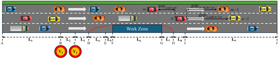
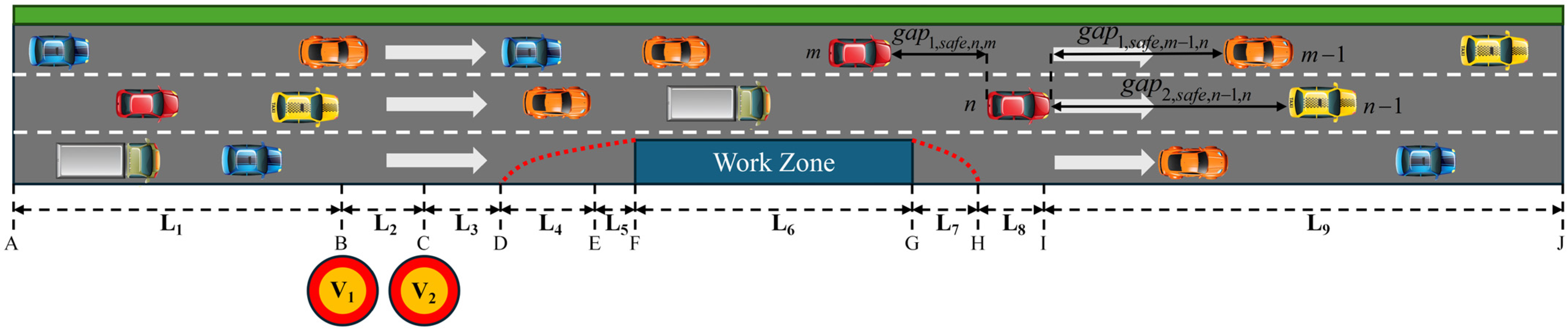
This study establishes an urban arterial road with a total length of 2 km as the road model where vehicles travel from left to right. Lane 3 is partially closed due to construction. Figure 1 shows the road map with the work zone. In accordance with relevant specifications [40], sections AB and HJ are normal driving sections with lengths of L₁ = 500 m and L₉ = 900 m respectively. Section BD serves as the warning area where speed limit signs V₁ = 50 km/h and V₂ = 40 km/h are installed at points B and C to ensure driving safety and prepare for subsequent lane changing to avoid the work zone. Among them, the length of section BC is L₂ = 150 m, and the length of section CD is L₃ = 150 m. Section DE is the upstream transition area. It has a length of L₄ = 100 m to meet the requirements for tapered sections. Vehicles in this area should change from lane 3 to lane 2 as soon as possible. If vehicles do not complete lane changing in section DE, they should brake and wait in the buffer section EF before changing to lane 2. Section EF has a length of L₅ = 50 m. This length ensures that vehicles do not collide with the work zone during braking. Section FG corresponds to the work zone with a length of L₆ = 50 m. A gate is installed at its midpoint to facilitate the access of transport trucks on lane 2 to the work zone. Section GH is the downstream transition area. It has a length of L₇ = 50 m to meet the requirements for reverse tapered sections. Lane 3 is reopened for traffic in this area. However, to ensure safety, the speed limit is removed after section HI with a length of L₈ = 50 m, and the speed is restored to 60 km/h.

Figure 1. Schematic layout of the study road segment with a work zone, showing the segment partitioning (L₁–L₉) and key locations (A–J).

3.2. Safe Distance

The safe distance is the required spacing between a leading vehicle and a following vehicle. This spacing prevents rear-end collisions when the leading vehicle performs emergency braking. It depends on the braking capacities of both the leading and following vehicles as well as the reaction time of the driver of the following vehicle. Therefore, the value of the safe distance varies under different car-following combinations. In this paper, to approximate real-world scenarios, a heterogeneous traffic flow composed of three types of vehicles is adopted, and the specific types and parameters are provided in Table 1.

Table 1. Vehicle types and relevant parameters.

Parameters	Car	Normal Truck	Transport Truck
Length	4 m	6.5 m	8 m
Maximum Acceleration	4 m/s2	2 m/s2	1.5 m/s2
Emergency Braking Deceleration	5 m/s2	3 m/s2	2.5 m/s2

The safe-distance criterion used in this study is constructed with reference to the formulation proposed by Gipps et al. [41]. In this paper, the Gipps-based idea is not directly used as a continuous trajectory update model. Instead, it is used to build a safety-oriented spacing criterion within the discrete CA framework. The resulting quantity is then used to evaluate car-following safety and lane-changing safety under different vehicle combinations:

$$ga{p}_{Lane,safe,n-1,n}=v_n(t){\mathsf{\tau }}_n+{\displaystyle \frac{v_n^2(t)}{2b_n}}-{\displaystyle \frac{v_{n-1}^2(t)}{2b_{n-1}}}$$

(1)

where $ga{p}_{Lane,safe,n-1,n}$ is the safe distance between the leading and following vehicles in the current lane, $ga{p}_{Lane,safe,m-1,n}$ and $ga{p}_{Lane,safe,n,m}$ are the safe distance between the vehicle in the current lane and the leading and following vehicles in the adjacent lanes. $v_n(t)$ is the speed of vehicle $\mathrm{n}$ at time $\mathrm{t}$, and $v_{n-1}(t)$ is the speed of vehicle $n-1$ at time $t$. $b_n,\hspace{0.33em}{b}_{n-1}$, as shown in Table 1, respectively represent the emergency braking deceleration of vehicle $n,n-1$, and ${\mathsf{\tau }}_{\mathrm{n}}$ is the driver’s reaction time under different car-following combinations. There are nine types of car-following combinations in this paper corresponding to nine reaction times, and the specific parameters are provided in Table 2.

Table 2. Reaction time under different car-following combinations [42].

	Car as Leader	Normal Truck as Leader
Car as follower	1.8 s	1.9 s
Normal Truck as follower	1.9 s	2 s
Transport Truck as follower	2 s	2.1 s

3.3. Lane-Changing Rules

The lane-changing rules for each section in Figure 1 are described below. These rules are based on three aspects. The first is safety. The second is potential speed and space benefit. The third is the traffic regulations in the work zone environment. In this paper, the traffic rules follow the relevant specifications [40]. Lane 1 only allows cars along the entire section. In the normal sections of lane 2, only cars are allowed. Only in section BG are normal trucks and transport trucks on lane 3 permitted to enter lane 2 for obstacle avoidance, and they shall return to lane 3 in a timely manner after point G. Therefore, lane-changing decisions in the proposed model are not triggered by a single condition. They are determined by the joint effects of local safety conditions, possible operational benefits, and section-dependent behavioral constraints.

Case 1: For the entire section of lane 1, as well as the normal sections, downstream transition zones, and termination zones on lanes 2 and 3 (i.e., Sections AB and GJ), lane-changing decisions are described by a two-phase mechanism and executed with a certain probability.

Phase 1 (preventive lane changing):

$$ga{p}_{Lane,n-1,n}\ge ga{p}_{Lane,safe,n-1,n}$$

(2)

Incentive criteria:

$$ga{p}_{Lane,n-1,n}-ga{p}_{Lane,safe,n-1,n}<v_n(t)-v_{n-1}(t)$$

(3)

$$ga{p}_{Lane,m-1,n}>ga{p}_{Lane,n-1,n}+{\alpha }_1$$

(4)

Safety criterion:

$$ga{p}_{Lane,n,m}\ge ga{p}_{Lane,safe,n,m}$$

(5)

Phase 2 (high-risk lane changing):

$$ga{p}_{Lane,n-1,n}<ga{p}_{Lane,safe,n-1,n}$$

(6)

Incentive criteria:

$$v_{n-1}(t)<v_n(t)$$

(7)

$$ga{p}_{Lane,m-1,n}\ge {\gamma }_1(ga{p}_{Lane,n-1,n}+{\alpha }_1)$$

(8)

Safety criterion: Equation (5) is adopted here.

In Case 1, a two-phase lane-changing mechanism is introduced to describe driver decisions under different risk levels. The two phases represent two typical trigger states during driving. Phase 1 corresponds to an early adjustment stage. At this stage, the immediate risk is still limited, but the driver may already perceive a possible loss of speed or space. Phase 2 corresponds to a stronger response stage. At this stage, the safety risk becomes more obvious, and the lane-changing demand becomes more urgent. Therefore, the two phases together describe how drivers respond to both potential risk and increasing risk.

It should be emphasized that there exists a scenario where both lane 1 and lane 3 meet the lane-changing conditions for the cars on lane 2 in case 1. On normal sections, the lane with a larger spacing will be selected for lane changing with a certain probability, as shown in Appendix A. On abnormal sections (i.e., Section BG), all vehicles are no longer allowed to enter lane 3.

Phase 1 represents an early adjustment stage. At this stage, the immediate safety risk is still limited. However, the current vehicle may already detect a possible loss of spacing or speed advantage. Equation (2) means that the current spacing is still larger than the safe distance. Equation (3) means that this spacing may shrink quickly when the current vehicle travels faster than the leading vehicle. To avoid unnecessary lane-changing triggers caused by small disturbances, Equation (4) introduces a stimulation factor. This factor is used as a behavioral control variable rather than a directly calibrated empirical quantity. It raises the trigger threshold and makes the lane-changing decision more selective. For leading vehicles of different types, different stimulation values are used to reflect different levels of perceived urgency.

Phase 2 represents a stronger adjustment stage. At this stage, the safety risk has become more obvious. Equation (6) shows that the actual spacing is smaller than the safe distance. Equation (7) shows that the current vehicle is still moving faster than the leading vehicle. These two conditions indicate that the rear-end collision risk is increasing. Therefore, Equation (8) introduces a discount coefficient, where ${\gamma }_1\hspace{0.33em}=\hspace{0.33em}0.9$, to reduce the trigger threshold. This setting allows the model to respond more sensitively in high-risk situations. It reflects the fact that safety becomes more important when the traffic condition becomes critical.

Case 2: Warning zone and upstream transition zone

For the lane changing from lane 3 to lane 2, the rules are modified as follows:

Incentive criteria:

$$ga{p}_{Lane,m-1,n}>\max (ga{p}_{changing},Lengt{h}_{vehicle})$$

(9)

Safety criterion:

$$ga{p}_{Lane,n,m}>{\gamma }_{2}ga{p}_{Lane,safe,n,m}$$

(10)

External stimulation on lane 3 increases as the numbers of low-speed and queued vehicles grow. Therefore, less stimulation is needed to reach the lane-changing threshold. In this scenario, the spatial benefit in Equation (9) and the safety guarantee in Equation (10) are used to define the minimum stimulation threshold. $ga{p}_{changing}$ is the minimum spacing that should be achieved on the adjacent lanes, and ${\gamma }_2$ is the discount coefficient. In the warning zone and upstream transition zone, $ga{p}_{changing}$ is set to 10 m and 7 m respectively, and ${\gamma }_2$ is set to 0.85. $Lengt{h}_{vehicle}$ is shown in Table 1. The parameter $ga{p}_{changing}$ denotes the minimum spacing that should be available on the adjacent lane before a mandatory lane-changing maneuver is considered behaviorally acceptable. It should be noted that $ga{p}_{changing}$ is not used as a collision-avoidance safe distance. Collision-avoidance safety is still evaluated by the Gipps-based safe-distance criterion in Equation (1) and by the spacing constraint with the following vehicle in the adjacent lane. Therefore, $ga{p}_{changing}$ should be interpreted as a section-dependent spatial-benefit and gap-acceptance threshold rather than as a substitute for the dynamic safety-distance calculation.

In the warning zone, vehicles are still relatively far from the lane closure and have more time and space to complete lane changing. Their lane-changing behavior is mainly preventive. Therefore, a larger value of $ga{p}_{changing} = 10 \mathrm{m}$ is adopted to avoid unnecessary lane changes caused by small spacing fluctuations. In the upstream transition zone, vehicles are closer to the closed lane section, and the mandatory lane-changing demand becomes stronger. Drivers are expected to accept a smaller available gap under this stronger external constraint. Therefore, a smaller value of $ga{p}_{changing} = 7 \mathrm{m}$ is adopted to represent more tolerant gap acceptance near the work zone bottleneck. These two values are representative behavioral settings for the studied work zone scenario rather than universally calibrated empirical constants.

Meanwhile, lane changing from lane 2 to lane 3 is prohibited, and the probability of lane changing from lane 3 to lane 2 is increased. Lane changing is activated for both normal trucks and transport trucks. The remaining lane-changing rules and probabilities remain unchanged until the downstream transition zone resumes its original state.

Case 3: Buffer zone on lane 3

Incentive criteria:

$$ga{p}_{Lane,m-1,n}>Lengt{h}_{\mathit{vehicle}}$$

(11)

Safety criterion:

$$ga{p}_{Lane,n,m}>v_m(t)$$

(12)

The stimulation caused by low-speed driving, stopping, or queuing has already exceeded the threshold. Therefore, lane changing occurs once the minor conditions in Equations (11) and (12) are met. Equation (11) requires spacing greater than the vehicle length, and Equation (12) ensures no collision with the following vehicle after the lane change, where $v_m(t)$ represents the speed of the following vehicle in the adjacent lane and the probability of lane changing from lane 3 to lane 2 is further increased. The parameter values of lane changing probabilities in cases 1 to 3 are listed in Appendix A.

3.4. Longitudinal Position Updating Rules

Compared with traditional CA models, such as the Nagel–Schreckenberg (NaSch) model, the proposed model does not use a fixed acceleration pulse for cars and normal trucks at each time step [43,44]. Instead, the speed change of these vehicles is determined adaptively. This design is based on a driving utility function that balances speed benefit and safety priority. Therefore, the longitudinal update process is more flexible in the studied work zone scenario. For transport trucks, the model still uses a simpler speed-update rule in section BG. This setting is used to reflect their larger mass and lower frequency of speed adjustment before entering the work zone.

Reward function:

$$R(a)=\left\{\begin{array}{l}\eta [v_0^2-{(v_{actual}-v_{desire})}^2] \mathrm{if} \eta \ge 0 or \eta <0 and v_{actual} < v_{desire} \hfill \\ \eta [v_0^2+{(v_{actual}-v_{desire})}^2] \mathrm{if} \eta <0 and v_{actual} \ge v_{desire} \hfill \end{array}\right.$$

(13)

where $\eta =ga{p}_{actual}-ga{p}_{safe}$, $ga{p}_{actual}$ is the distance between the vehicle and the nearest obstacle ahead, where the obstacle can refer to other vehicles or the work zone. $ga{p}_{safe}$ is the safe distance from the obstacle ahead, which can be calculated by Equation (1). $v_0$ is the normal road speed limit. $v_{actual}$ is the current actual operating speed of the vehicle, and $v_{desire}$ is the current road speed limit.

Equation (13) is used to calculate the acceleration $a_{reward}$ within a certain spatial range. $a_{reward}$ is the point that maximizes $R(a)$ in the interval $[a(t-1)-\epsilon ,a(t-1)+\epsilon ]$, where $a(t-1)$ is the acceleration at time $t-1$ with $a(0)=0 \mathrm{m}/{\mathrm{s}}^2$ and $\epsilon$ is a value introduced to limit excessive changes in acceleration, and here, $\epsilon =1 \mathrm{m}/{\mathrm{s}}^2$ is adopted. If beyond a certain spatial range (i.e., $ga{p}_{actual}>50\mathrm{m}$), the maximum acceleration $a_{\mathrm{acc},\max }$ of the corresponding vehicle in Table 1 is adopted.

Therefore, the longitudinal position updating rules of the CA model in this paper are as follows.

Select acceleration/deceleration:

$$a(t)=\left\{\begin{array}{l}\min (a_{acc,\max },a_{reward}) if a_{reward}>0 and ga{p}_{actual}\le 50 \mathrm{m} \hfill \\ \max (a_{dec,\max },a_{reward}) if a_{reward}<0 and ga{p}_{actual}\le 50 \mathrm{m} \hfill \\ a_{acc,\max } if ga{p}_{actual}>50 \mathrm{m} \hfill \end{array}\right.$$

(14)

Speed update:

$$v(t+1)=v(t)+a(t)$$

(15)

Position update:

$$x(t+1)=x(t)+v(t+1)$$

(16)

where, $x(t)$ is the position of the vehicle at time $t$, and $x(t+1)$ is the position of the vehicle at time $t+1$.

4. Simulation Results and Discussions

4.1. Simulation Configurations

This study examines the characteristics of the proposed model and investigates traffic impacts under the coupled effects of transport trucks and the work zone. Simulations are conducted under both periodic boundary conditions and open boundary conditions. The length of a single cell is set to $L_{\mathrm{c}ell}=0.5 \mathrm{m}$, and road settings refer to Section 3.1. Vehicle-related parameters are listed in Table 1.

The behavior-related parameters used in the model should be interpreted as representative control variables for a typical urban work zone scenario rather than as fully calibrated empirical constants. The stimulation thresholds are used to describe the level of perceived urgency required to activate early lane-changing adjustment. Larger threshold values indicate more conservative responses, whereas smaller values indicate earlier responses to environmental or car-following disturbances. The discount coefficients are introduced to relax the trigger thresholds under higher-risk conditions, so that the model can represent more sensitive driver reactions when the available spacing becomes insufficient or when the vehicle approaches the closed-lane section. The minimum spacing requirements in the warning and upstream transition zones are used as section-dependent spatial-benefit and gap-acceptance thresholds, while collision-avoidance safety is still governed by the Gipps-based safe-distance criterion. The lane-changing probabilities are used to represent the stochastic execution of lane-changing decisions after the deterministic incentive and safety conditions are satisfied. Therefore, these parameters control behavioral tendency and disturbance intensity in the numerical experiment, rather than providing a site-specific calibration for a particular field work zone.

4.2. Simulation Results in the Periodic Boundary Condition

The periodic boundary condition is used here as a benchmark setting to examine the endogenous traffic-phase characteristics generated by the proposed EIBC model. Under this condition, the total number of vehicles in the system is fixed, and the influence of stochastic upstream arrival and downstream discharge is excluded. Therefore, the periodic boundary results are mainly used to identify the fundamental diagram, metastable behavior, and typical F → S and S → J transition mechanisms under controlled density conditions. They should not be interpreted as a complete representation of real urban work zone operation, which is better described by the open boundary simulations in Section 4.3.

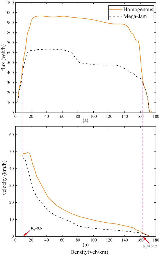
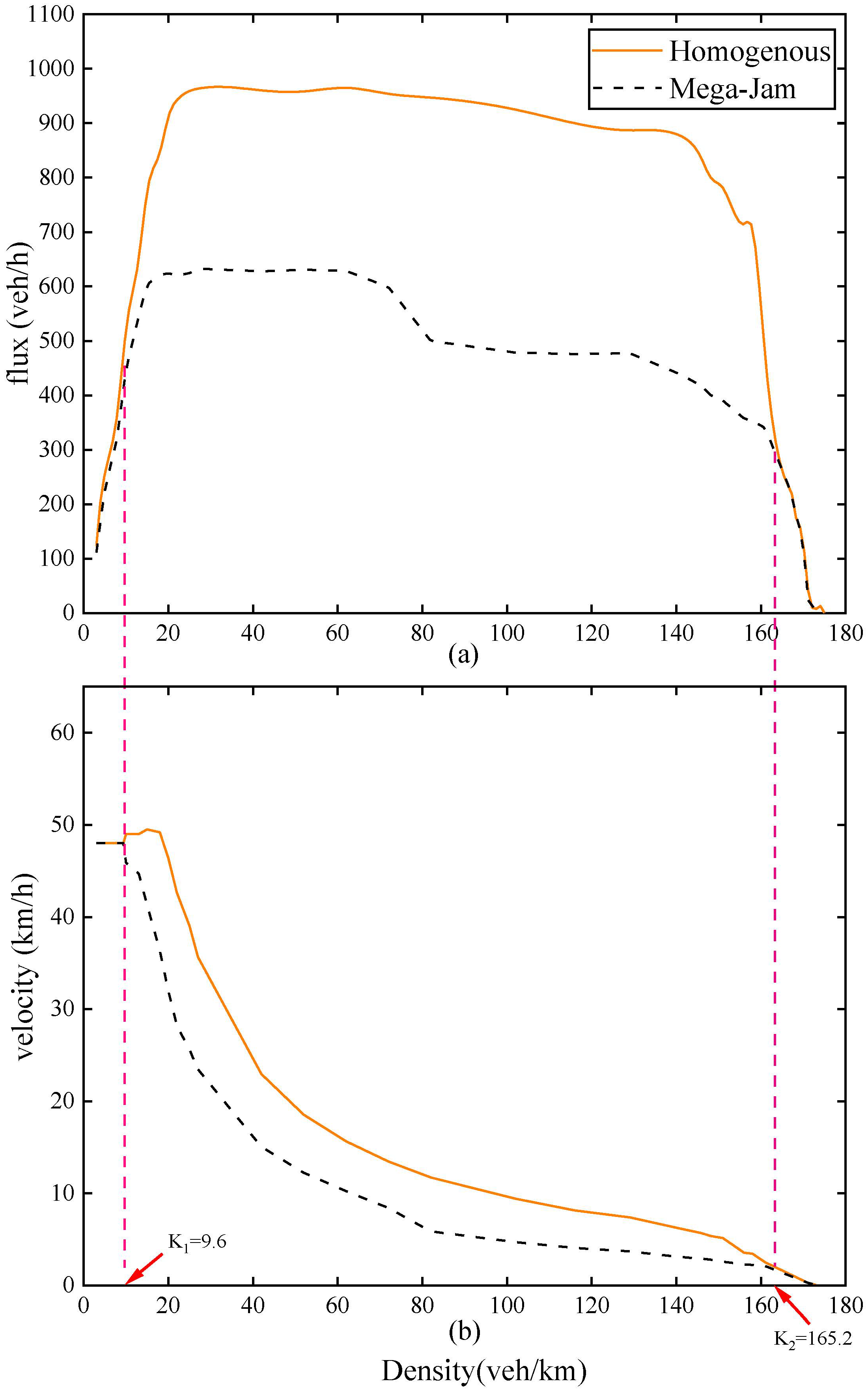
The periodic boundary condition means that, after a vehicle exits the end of the road, it will re-enter the system from the starting point. In this paper, the model is run under two types of initial conditions for periodic boundaries: initial uniform distribution and initial dense distribution. Only cars are used to create a homogeneous background traffic flow and generate a benchmark fundamental diagram without vehicle-type disturbances. This setting allows the hysteresis characteristics caused by the model’s endogenous mechanism to be identified more clearly. To plot the fundamental diagram, the normalized density is gradually increased from 0 to 1 in steps of 0.01. A simulation experiment of 10,000 s is conducted at each density level. The traffic system is not stable at the beginning of the simulation, so a warm-up period is required. Therefore, the first 4000 s of data are discarded in each experiment, and only flow, speed, and density in the subsequent stable stage are recorded. The fundamental diagram produced by the model is shown in Figure 2a,b. The orange curve corresponds to the results under the initial uniform distribution, and the black curve corresponds to the results under the initial dense distribution.

Figure 2. Fundamental diagram. (a) is averaged flow–density diagram, and (b) is averaged velocity–density diagram.

Under the low-density condition where K < K₁, vehicles on lane 3 must change to lane 2 in a timely manner in order to pass the work zone. Meanwhile, there is sufficient space on lane 1 and lane 2 for all vehicles to operate at the maximum speed limit required by the area. Under this scenario, after a period of warm-up and the system stabilizes, vehicles will concentrate on lane 1 and lane 2 and travel in a stable free-flow state, as shown in Figure 3. In contrast, there are no longer any vehicles traveling on lane 3 after the system becomes stable. Therefore, no sustained trajectories are observed on lane 3 near the closed section.

Figure 3. Time–space plot at K = 7 veh/km with uniformly distributed initial conditions: (a) Lane 1; (b) Lane 2.

When density enters [K₁, K₂], free flow can still be maintained on average, but the traffic state becomes metastable. Near the fixed bottleneck created by the work zone, synchronized flow (S) is more likely to be triggered by nucleation. This nucleation can cause local traffic breakdown, corresponding to an F → S phase transition. This mechanism causes the two-dimensional scatter region in Figure 2 to exhibit a phenomenon of splitting from the middle within this density range. The upper branch corresponds to the evolutionary path under the initial uniform distribution. It shows a mixed state where free flow and S coexist, as shown in Figure 4. The lower branch corresponds to the evolutionary path under the initial dense distribution. It shows a mixed state where S and WMJ coexist, as shown in Figure 5.

Figure 4. Time–space plot at K = 27.17 veh/km with uniformly distributed initial conditions: (a) Lane 1; (b) Lane 2; (c) Lane 3.

Figure 5. Time–space plots at K = 27.17 veh/km with densely distributed initial conditions and at K = 171 veh/km. (a) Lane 1; (b) Lane 2; (c) Lane 3; (d) Lane 1; panels (a–c) are obtained from simulations at K = 27.17 veh/km with densely distributed initial conditions, and panel (d) is obtained from simulations at K = 171 veh/km.

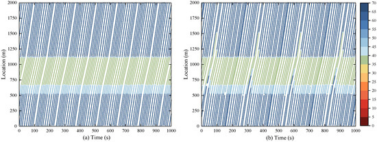
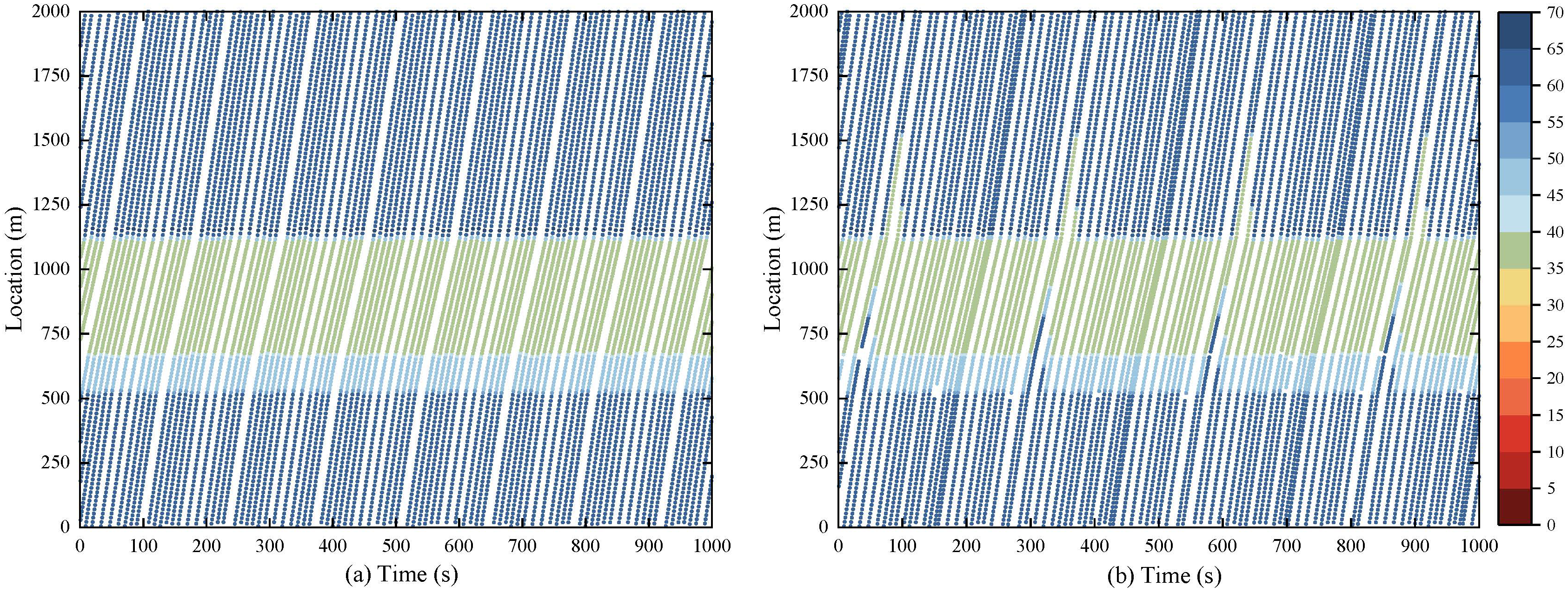
As shown in Figure 4, the lane reduction at the work zone triggers a low-speed zone upstream of the bottleneck from 950 m to 1000 m. Its downstream front is basically locked to the bottleneck position. At this front, vehicles accelerate from S to downstream free flow. At the upstream front, vehicles decelerate from upstream free flow to enter S. This forms a typical F and S coexisting state. Further comparison of each lane shows that lane 1 continuously bears merging disturbances and lacks effective diversion channels. Therefore, lane 1 is more prone to compressed available gaps and speed restrictions under medium-density operating conditions. At most spatiotemporal positions adjacent to the work zone, the speed adaptation effect is more likely to prevail over the over-acceleration effect. This increases the probability of F → S nucleation and promotes the evolution of S-type congestion patterns. This is manifested as the generation of multiple SPs in Figure 4a. As S propagates upstream, the direct impact of the geometric constraints of the work zone on upstream traffic gradually weakens, enabling the over-acceleration effect to dominate at certain random spatiotemporal positions. The MSP in Figure 4a can be interpreted as an MSP formed by the phased dominance of the speed adaptation effect. It undergoes random S → F reversion during further upstream propagation and eventually dissolves into free flow. The composite SP in Figure 4a can be understood as an intermittent alternation of SPs. This alternation is caused by temporal variations in flow rate and disturbance input at the bottleneck. This interpretation is consistent with Kerner’s explanation of the formation mechanism of composite SPs [44].

By contrast, the low-speed zone of lane 2, as shown in Figure 4b, is also attached to the upstream of the bottleneck, but its upstream boundary mainly exhibits fluctuations within a limited range and is more localized overall without continuously expanding upstream like lane 1. The reasons are as follows. Lane 2 continuously receives speed disturbances and additional inflow from mandatory merging from lane 3. However, under the initial uniform distribution in this density interval, lane 1 retains relatively sufficient available space. This enables part of the traffic pressure on lane 2 to be released through the transfer of vehicles to lane 1, thereby reducing the growth intensity of disturbance nuclei and inhibiting the continuous expansion of the S region. Speed limit signs are installed at the starting point of the warning zone at Point B in Figure 1. They induce excessive deceleration with a certain probability. Therefore, LSPs are more likely to form at this location. As for lane 3, as shown in Figure 4c, its spatiotemporal structure is mainly dominated by the queue process of merging–waiting–dissipating due to the constraints of construction closure and mandatory lane-merging rules. The missing or broken trajectories near the closed zone should be understood as a direct result of geometric constraints and control rules, rather than a characterization of the internal structure of S itself.

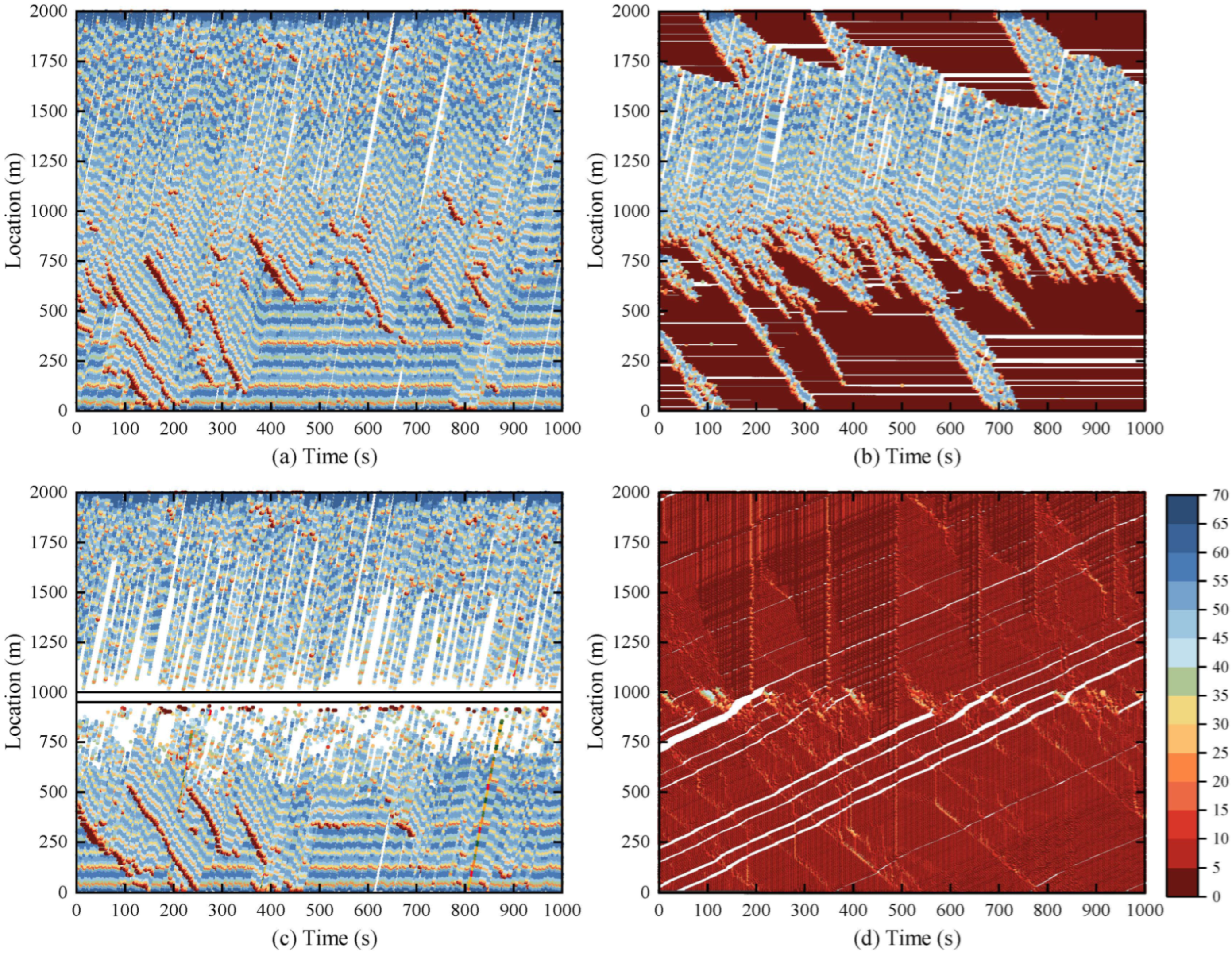
Figure 5 presents the spatiotemporal evolution characteristics of road traffic flow under the condition of initial dense distribution. Compared with the initial uniform distribution scenario, the number of vehicles queuing to merge near the work zone on lane 3, as shown in Figure 5c, is significantly reduced. This is because the initial vehicle spacing is smaller, stimulating vehicles on lane 3 to initiate lane changing earlier. Figure 5b shows that lane 2 exhibits the spatiotemporal structure of WMJs. Figure 5a shows that lane 1 is mainly characterized by large-scale synchronized flow. Lane 1 is also superimposed with a coupled GP spatiotemporal mode embedded with local congestion clumps. This difference can be explained from two aspects. One aspect is the enhanced disturbance sensitivity induced by the initial dense state. The other aspect is the continuous external disturbances introduced by mandatory lane merging at the work zone. Under the initial dense condition, vehicle spacing is smaller, and car-following coupling is stronger. Therefore, the system is more prone to forming a metastable S background near the bottleneck. The construction closure forces vehicles on lane 3 to merge into lane 2 continuously. Lane 2 receives high-intensity mandatory additional inflow and corresponding speed disturbance input from lane 3. This process is usually accompanied by significant deceleration and yielding behaviors. Therefore, it becomes easier to form disturbance nuclei dominated by excessive deceleration in the S background of lane 2. This can trigger the S → J phase transition.

When congestion clumps reach a certain intensity, they become self-sustaining and propagate upstream at an approximately constant speed. They ultimately form a WMJ-dominant structure on lane 2, as shown in Figure 5b. In contrast, due to the smaller initial vehicle spacing and the absence of mandatory lane-merging impacts, Lane 1 is less affected by the congestion and flow redistribution of lane 2, thus maintaining a large-scale S. During periods dominated by random disturbance and the excessive deceleration mechanism, the S → J nucleation process may occur within the S background. This process can further form a GP coupled spatiotemporal pattern in which S and local congestion clumps coexist, as shown in Figure 5a. When K > K₂, the system stably enters a severe congestion state dominated by WMJs. This state is insensitive to the initial distribution form regardless of whether the initial distribution is uniform or dense, and large-scale and persistent WMJ structures will emerge. The dominant congestion patterns of each lane show strong consistency in the macro-spatiotemporal structure under high-density conditions. Therefore, the spatiotemporal evolution of lane 1 can reflect the key characteristics of the system entering the WMJ-dominated state. Thus, Figure 5d only presents a representative speed spatiotemporal diagram of lane 1 under high-density operating conditions. In the figure, the low-speed congestion area extensively occupies the study section for a long period of time. A typical upstream-propagating diagonal band structure is observed. This structure indicates that this density has developed into a WMJ-dominated congestion state covering the full road section.

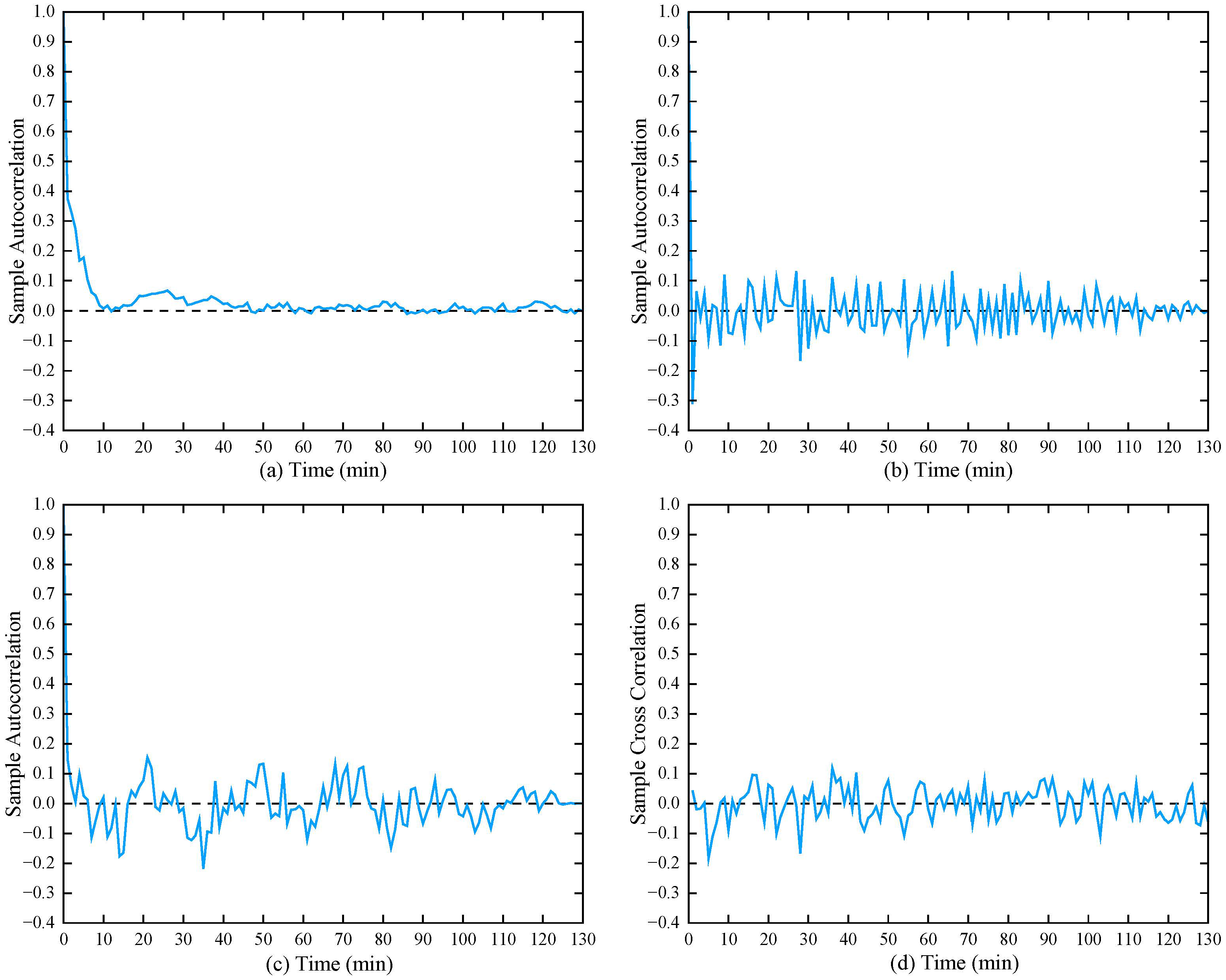
To further verify the evolutionary characteristics of S identified in Figure 4 from a statistical perspective, the present study adopts the autocorrelation and cross-correlation analysis methods proposed in [45]. Virtual detectors are deployed at point D, as shown in Figure 1. Time series of traffic flow, spatial average speed, and density are collected continuously for 130 min under the operating condition of K = 27.17 veh/km. As shown in Figure 6, when the lag time is in a large range, the autocorrelation coefficients of density, flow, and speed decay rapidly fluctuate slightly around 0. Meanwhile, the cross-correlation coefficient between flow and speed does not exhibit a stable and significant deviation but fluctuates randomly around 0. At this density level, the macroscopic variables of the traffic system do not show stable periodicity or strong coherent relationships on a long-time scale. This is consistent with the characterization of the statistical characteristics of S in [45]. The aforementioned correlation analysis provides statistical support that the spatiotemporal structure shown in Figure 4 belongs to the S state. It also shows that the evolution of congested states in the proposed model is consistent with Kerner’s three-phase traffic flow theory framework.

Figure 6. Panels (a), (b), and (c) show the autocorrelation functions of density, flow, and speed, respectively. Panel (d) shows the cross-correlation function between flow and speed.

4.3. Simulation Results in the Open Boundary Condition

Under the open boundary condition, this study aims to distinguish the impacts of the work zone and transport trucks on traffic flow evolution. The overall road operating conditions are kept as consistent as possible. Therefore, the system average density is controlled near the interval from K₁ to K₂ through the inlet deployment mechanism. Specifically, random deployment rules are set at point A of the road entrance, as shown in Figure 1, and conventional vehicles (cars and normal trucks) are injected into the system with a deployment probability $p_{create}$ when the entrance meets spatial constraint conditions such as the minimum safety gap. Meanwhile, a fixed number n (n = 0, 1, 2, 3) of transport trucks are deployed at the entrance of lane 3 at 500 s into the simulation time period corresponding to the spatiotemporal diagram. Transport truck initial speed is uniformly set to 36 km/h, and they will wait for T seconds at the entrance of the work zone before entering it, where T is set to 20 s to avoid further density increase leading the system to enter the severe congestion state where K > K₂. The deployment probability is set to 0.4 when K < K₂ and 0.1 when K ≥ K₂, thereby achieving effective constraint on the section density. The initial speed of conventional vehicles is set to $v_0=v_{ga\mathrm{u}ss}$, where $v_{ga\mathrm{u}ss}$ is the random free speed following a gaussian distribution (truncated at the speed limit). The above settings ensure controllable density and boundary input. Under these conditions, the independent effect of the work zone and the coupling effect between the work zone and transport trucks can be investigated. These effects are examined in terms of traffic flow phase transitions and the evolution of congestion structures.

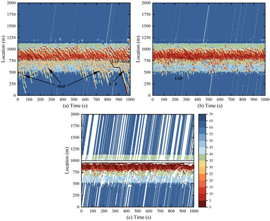
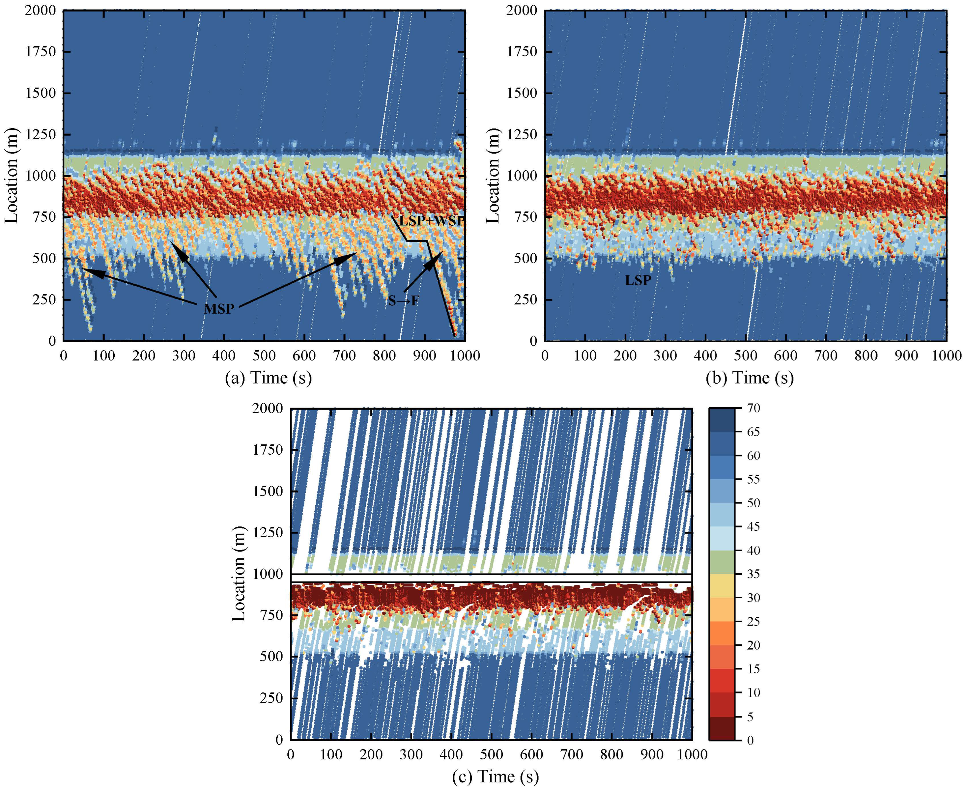
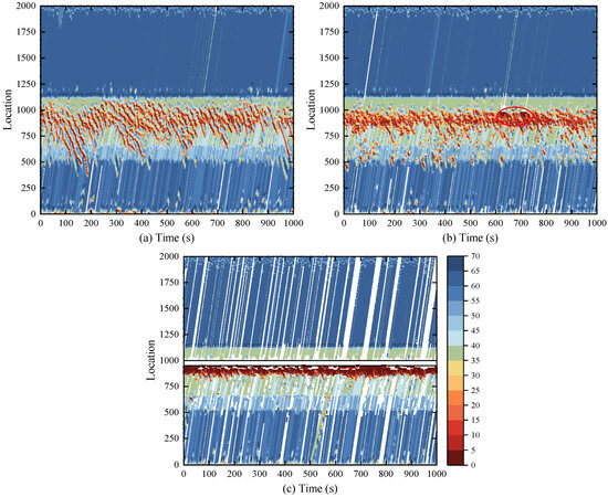
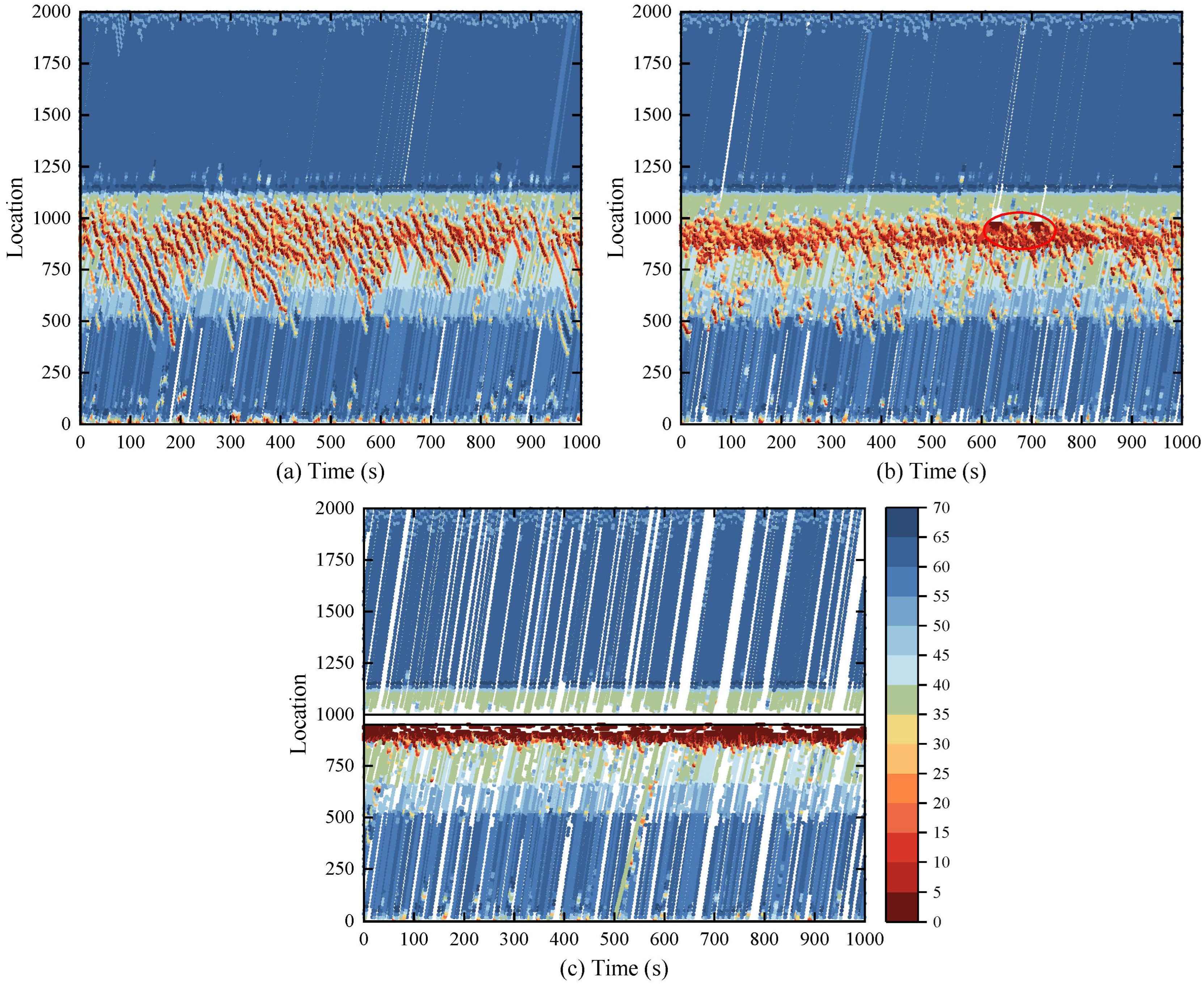
Within the time interval of 0–500 s, the non-free flow generated on lane 1 in Figure 7 is attributed to the inability to dissipate the spillover of pressure from lane 2. Compared with periodic boundary conditions, open boundary conditions feature a more random number of deployed vehicles and an uneven spatiotemporal distribution of inter-vehicle distances. Additionally, considering the randomness of the spatiotemporal competition between the speed adaptation effect and the over-acceleration effect, the non-free flow of lane 1 within the same regional range (500 m–1000 m) exhibits different traffic flow patterns.

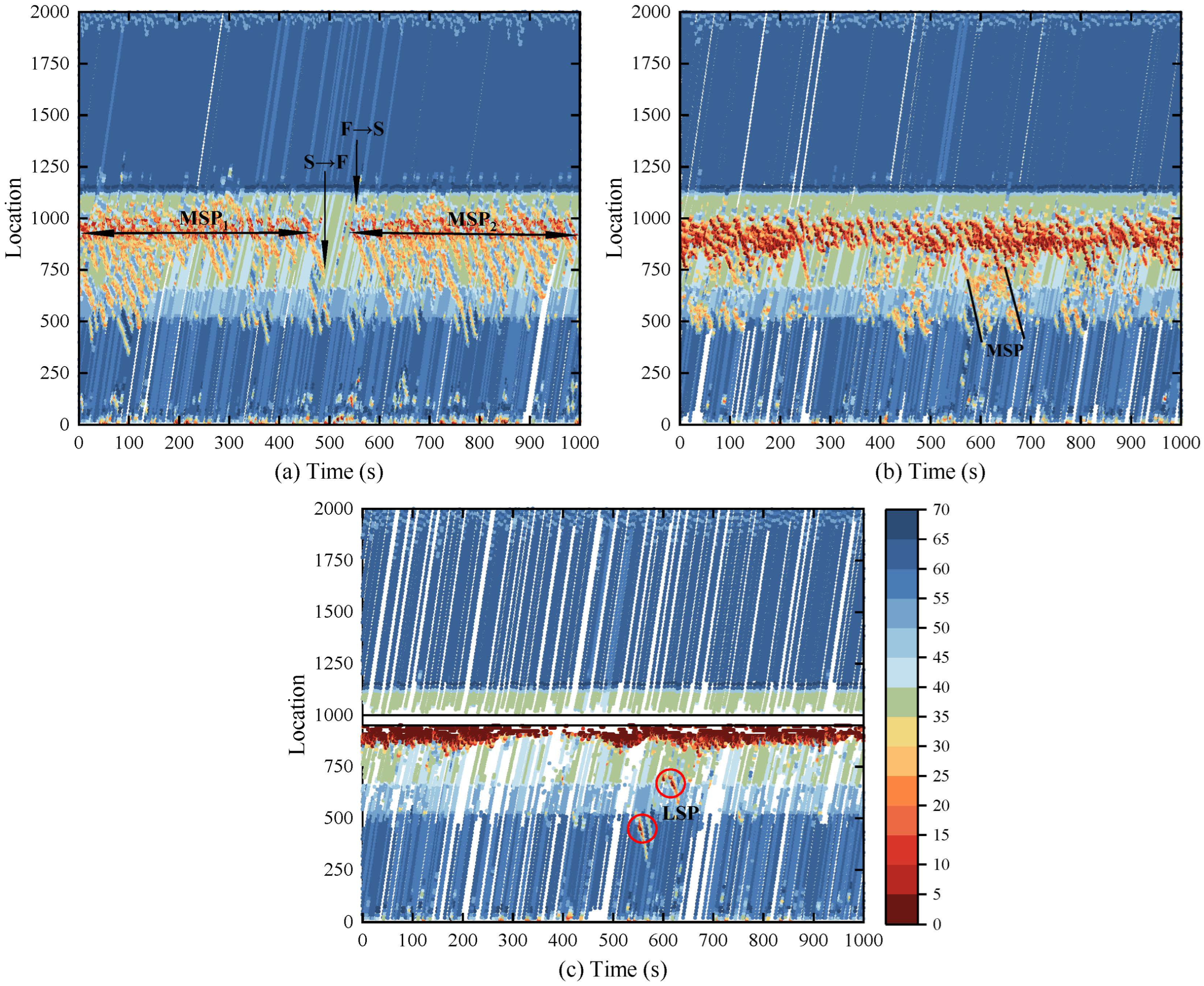
Figure 7. Time–space plots under work zone effects with n = 0: (a) Lane 1; (b) Lane 2; (c) Lane 3.

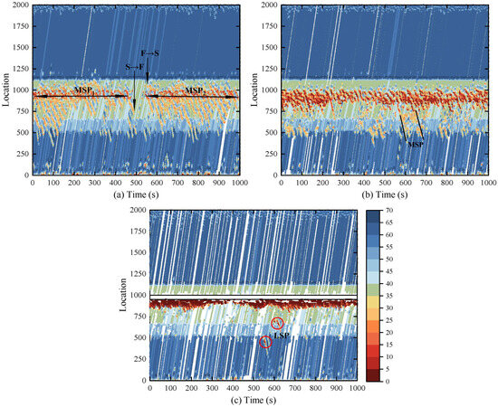
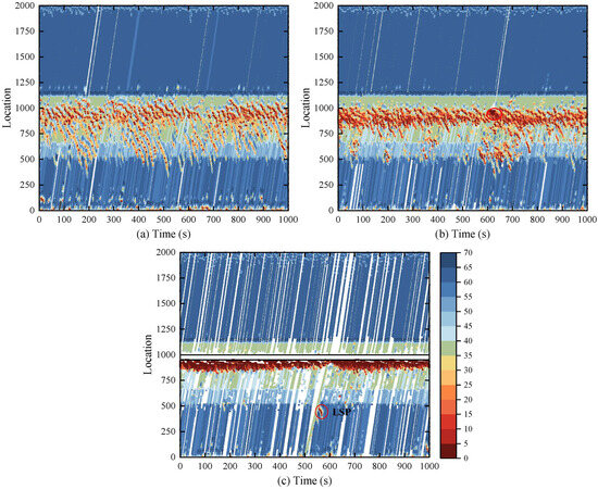
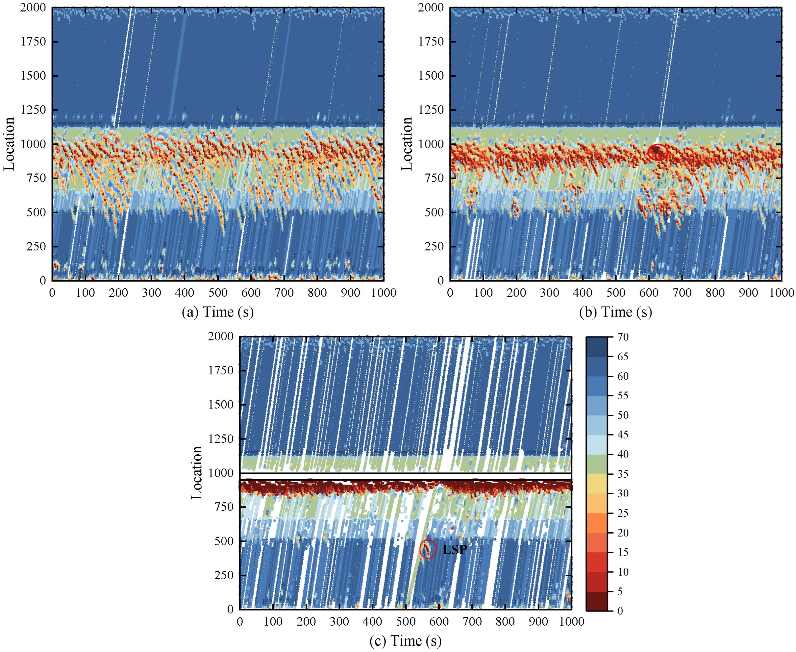
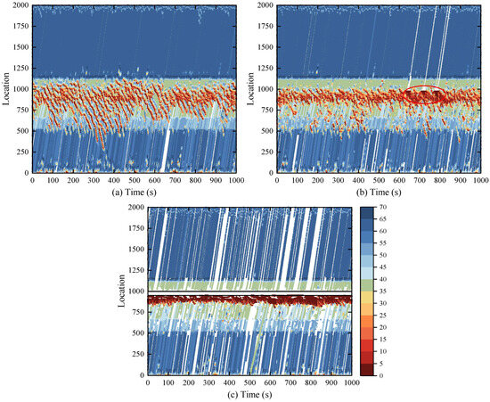
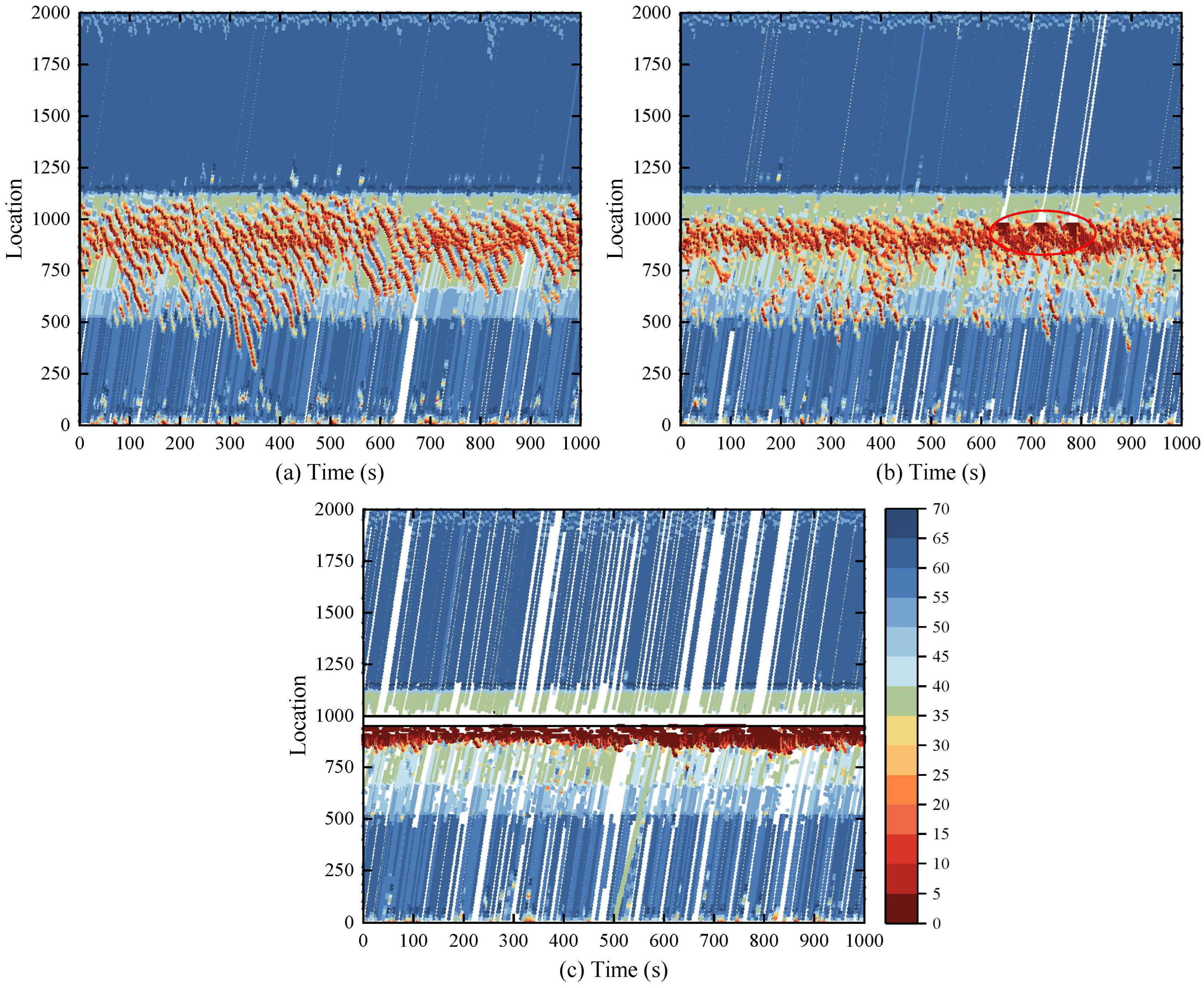
The following comparisons are qualitative in nature. They are intended to examine whether the proposed model can reproduce spatiotemporal pattern types that are consistent with empirical observations reported in the three-phase traffic theory literature. Therefore, the results should be interpreted as qualitative consistency validation of the underlying mechanism rather than as direct trajectory-level empirical validation. Figure 7a shows that two dissolvable MSPs are observed within this range. These MSPs are accompanied by S → F and F → S transitions. This is consistent with the results in Figure 9.6 of [39] based on real traffic data. Compared with the results shown in Figure 7a, low-intensity, low-speed nuclei are gradually generated in the synchronized flow depicted in Figure 8a, and these nuclei will gradually dissolve into the S. However, the low-speed nuclei in Figure 9a and Figure 10a have higher intensity and continuously develop, resulting in a large number of GPs.

Figure 8. Time–space plots under work zone effects with n = 1: (a) Lane 1; (b) Lane 2; (c) Lane 3.

Figure 9. Time–space plots under work zone effects with n = 2: (a) Lane 1; (b) Lane 2; (c) Lane 3.

Figure 10. Time–space plots under work zone effects with n = 3: (a) Lane 1; (b) Lane 2; (c) Lane 3.

Figure 7b shows that lane 2 exhibits MSPs with a wider scope and longer duration within the range of 500 m to 750 m. This is the combined result of the spatiotemporal dominance of the speed adaptation effect and the upstream propagation of downstream congestion. Similar phenomena can be observed in Figure 8b and Figure 10b, but the latter two are more characterized by spontaneous nucleation-type phase transitions.

Figure 7c shows that the LSP on lane 3 is mainly caused by mandatory speed reduction and lane-merging waiting at the work zone. During lane-merging waiting, leading vehicles decelerate and induce a chain reaction in following vehicles. As a result, local synchronized flow is generated. Figure 8c shows that the LSP is triggered by the operation of transport trucks. This phenomenon is consistent with the results in Figure 7 of [28]. Transport trucks may merge into the work zone and temporarily compress acceptable gaps. They also block part of the traffic flow. Therefore, lane-changing demand to lane 1 increases. As the number of merged vehicles increases, the growth intensity and duration of disturbance nuclei in lane 2 increase accordingly. Therefore, S → J phase transitions are more likely to occur and expand within a certain spatiotemporal range. The above results verify the ability of the EIBC model to characterize microscopic interactions and congestion structures at work zone bottlenecks under more realistic open system conditions. The results also provide a reference basis for optimizing lane-merging organization and managing the entry of transport trucks.

To further clarify the empirical relevance of the simulated patterns, the main spatiotemporal structures obtained under the proposed EIBC model are compared qualitatively with the empirical pattern categories reported in the three-phase traffic theory literature. The comparison is not intended as a trajectory-level calibration against a specific field dataset. Instead, it examines whether the simulated traffic states reproduce the characteristic morphology and evolution mechanisms of empirically observed congested patterns.

First, the self-sustained low-speed bands shown in Figure 5b,d propagate upstream while maintaining a relatively stable spatiotemporal structure. This feature is consistent with the definition of wide moving jams, whose downstream front is not fixed at the bottleneck and can continue to propagate upstream through the traffic stream. Second, the bottleneck-attached low-speed regions on lane 3 in Figure 7c and Figure 8c are consistent with localized synchronized patterns. Their downstream fronts remain constrained by the work zone bottleneck, while the upstream extent remains limited within a local range. Third, the dissolvable synchronized-flow regions shown in Figure 7a,b exhibit moving synchronized-pattern characteristics because they are accompanied by alternating F → S and S → F transitions and may dissipate during upstream propagation. Finally, the more developed congestion structures in Figure 9a and Figure 10a can be interpreted as general congested patterns, in which local moving jams emerge and propagate within a synchronized flow background.

This qualitative comparison indicates that the EIBC model can reproduce not only traffic breakdown near the work zone bottleneck but also the main spatiotemporal pattern types associated with synchronized-flow evolution. Therefore, the model provides a mechanism-oriented representation of empirical three-phase traffic phenomena under urban work zone constraints.

4.4. Sensitivity Analysis of Key Behavioral Parameters

To further clarify the role of the newly introduced behavioral control variables in the proposed EIBC model, this study conducts a local sensitivity analysis under the representative open boundary work zone scenario. The analysis focuses on two parameters, namely ${\gamma }_1$ and $\alpha$. This choice is made because these two variables directly govern the two-phase lane-changing mechanism introduced in the model. Specifically, ${\gamma }_1$ controls the threshold relaxation in the high-risk lane-changing stage, whereas $\alpha$ scales the stimulus-related threshold in the early adjustment stage. By contrast, the remaining thresholds and probabilities are retained here as representative scenario settings. Therefore, the present sensitivity analysis is intended to examine the robustness of the core behavioral mechanism rather than to provide a full-parameter calibration study.

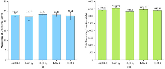
For each parameter setting, three indicators are examined: the F → S nucleation probability, the mean speed at Detector D during the analysis period, and the equivalent hourly total lane-change rate during the analysis period. The tested cases include the baseline setting, a lower and a higher ${\gamma }_1$, and a lower and a higher $\alpha$ scaling factor. The results are summarized in Table 3 and Figure 11a,b.

Table 3. Local sensitivity analysis of key behavioral parameters under the representative open boundary work zone scenario.

Setting	${\mathit{\gamma }}_1$	$\mathit{\alpha }$	F → S Nucleation Probability	Mean Speed at Detector D (km/h)	Total Lane-Change Rate (Events/h)
Baseline	0.9	1	1	23.02 ± 0.79	3435.89 ± 43.72
Low ${\gamma }_1$	0.85	1	1	22.17 ± 1.99	3534.73 ± 54.15
High ${\gamma }_1$	0.95	1	1	23.33 ± 0.78	3311.20 ± 34.67
Low $\alpha$	0.9	0.9	1	23.19 ± 0.82	3459.51 ± 48.08
High $\alpha$	0.90	1.10	1.00	22.61 ± 1.79	3385.11 ± 45.21

Figure 11. Sensitivity analysis under the representative open boundary work zone scenario: (a) mean speed at Detector D during the analysis period; (b) equivalent hourly total lane-change rate during the analysis period. Error bars denote standard deviations across repeated simulation runs.

As shown in Table 3, the F → S nucleation probability remains equal to 1.00 for all five settings. This indicates that, under the present open boundary input condition, the system is already located in a robust nucleation regime. Therefore, within the tested parameter range, the parameter variation does not change whether synchronized flow is nucleated. Instead, it mainly affects the operational characteristics of traffic after nucleation has already occurred.

Among the tested parameters, ${\gamma }_1$ exhibits the strongest influence. When ${\gamma }_1$ is reduced from 0.90 to 0.85, the mean speed at Detector D during the analysis period decreases from 23.02 ± 0.79 km/h to 22.17 ± 1.99 km/h, whereas the equivalent hourly total lane-change rate increases from 3435.89 ± 43.72 events/h to 3534.73 ± 54.15 events/h. By contrast, when ${\gamma }_1$ is increased to 0.95, the mean speed rises to 23.33 ± 0.78 km/h, and the equivalent hourly total lane-change rate decreases to 3311.20 ± 34.67 events/h. This tendency suggests that ${\gamma }_1$ exerts the strongest control over post-nucleation traffic operation among the tested parameters. A smaller ${\gamma }_1$ lowers the effective threshold in the unsafe lane-changing stage, makes reactive lane-changing maneuvers more likely near the bottleneck, and consequently enhances the lateral disturbance input to the traffic stream. A larger ${\gamma }_1$ produces the opposite effect, suppresses such high-risk lane-changing reactions, and results in a more stable local operating state.

The influence of $\alpha$ is weaker but still meaningful. When $\alpha$ is reduced from 1.00 to 0.90, the mean speed at Detector D increases slightly to 23.19 ± 0.82 km/h, and the equivalent hourly total lane-change rate also increases slightly to 3459.51 ± 48.08 events/h. When $\alpha$ is increased to 1.10, the mean speed decreases to 22.61 ± 1.79 km/h, and the equivalent hourly total lane-change rate decreases to 3385.11 ± 45.21 events/h. This result suggests that $\alpha$ mainly acts as a secondary regulator of the early adjustment stage. A smaller $\alpha$ facilitates earlier lane-changing adjustments before the traffic state becomes more critical. Under the present scenario, these earlier adjustments slightly improve the local speed level, even though the total lane-changing activity also increases. By contrast, a larger $\alpha$ makes the early response more conservative and tends to worsen the local operating state near the bottleneck.

In addition, the larger speed standard deviations under the low ${\gamma }_1$ and high $\alpha$ settings imply that these two parameter combinations lead to a more disturbance-sensitive traffic state. By comparison, the high ${\gamma }_1$ case not only yields the highest Detector D speed but also shows a relatively small standard deviation, which indicates a more stable local operating condition. Overall, the present sensitivity analysis shows that the behavioral parameters mainly regulate the intensity of post-nucleation traffic interactions under the representative open boundary work zone scenario. Within the tested parameter range, the sensitivity strength can be summarized as ${\gamma }_1>\alpha$.

Finally, it should be emphasized that the current scenario is already located in a robust F → S nucleation regime. Therefore, the present analysis mainly reveals the dependence of post-nucleation traffic operation on the behavioral control variables, rather than probability-level differences in whether nucleation occurs. A broader sensitivity study closer to the nucleation threshold may be conducted in future work to further distinguish probability-level effects.

5. Conclusions

This paper develops an improved cellular automaton model called EIBC for the analysis of traffic evolution near an urban work zone bottleneck. The model incorporates traffic-rule constraints and environment-related driving information into the lane-changing and speed-adjustment processes. Simulations are carried out under two boundary conditions on a three-lane urban road with a construction zone. The results show that the EIBC model can qualitatively capture the interaction between speed adaptation and over-acceleration near the bottleneck. The model can also reproduce the corresponding synchronized-flow-related congestion patterns under the studied scenario. In this sense, the proposed model provides a mechanism-oriented framework for interpreting traffic evolution near urban work zones within the context of Kerner’s three-phase traffic theory.

This paper also discusses transport trucks as a secondary external disturbance source under open boundary conditions with controllable input. The results show that a small number of transport trucks can trigger local synchronized-flow disturbances near the work zone. Under certain operating conditions, they can increase the growth intensity of disturbance nuclei. They can also prolong low-speed operation and enlarge the affected area. This finding suggests that work zone management should pay attention to heavy-vehicle entry timing and scheduling, in addition to lane occupancy and lane-merging organization.

This study still includes several idealized assumptions. The layout of each functional zone in the work zone is fixed, and the analysis is conducted for a three-lane urban road with a partial closure of lane 3 and prescribed speed-limit and rules. The current model also does not consider differences in information availability under vehicle-to-vehicle communication conditions. In addition, the parameter settings are used to describe a representative scenario rather than a fully calibrated field case. Therefore, the conclusions should be interpreted at two different levels. At the mechanism level, the results suggest that mandatory lane changing near a fixed work zone bottleneck can trigger localized synchronized flow; that the competition between speed adaptation and over-acceleration can generate F → S, S → F, and S → J transitions; and that transport truck entry can act as a secondary disturbance source that amplifies low-speed nuclei near the bottleneck. These mechanisms are expected to be relevant to similar lane-closure bottleneck scenarios. By contrast, the specific critical densities, the spatial range and duration of the congested patterns, and the quantitative influence of transport trucks are closely related to the three-lane road layout, the functional-zone lengths, the speed-limit settings, the lane-use rules, and the prescribed truck-entry assumptions adopted in this paper. Future work can consider more diverse work zone layouts, heterogeneous traffic compositions, broader global sensitivity analysis under near-threshold inflow conditions, and empirical calibration using field trajectories or connected-vehicle data. Furthermore, information-driven lane-changing and longitudinal control rules can be extended under connected-vehicle conditions to improve the engineering applicability of the model.

References

- Yu, M.; Zheng, C.; Ma, C. Analysis of Injury Severity of Rear-End Crashes in Work Zones: A Random Parameters Approach with Heterogeneity in Means and Variances. Anal. Methods Accid. Res. 2020, 27, 100126. [Google Scholar] [CrossRef] [Scilit]
- Duan, K.; Yan, X.; Ma, L.; Hang, J.; Li, X. A Multistage Analytic Model of the Longitudinal and Lateral Acceleration during Lane Changing in Work Zone Areas with the Aid of a Driving Simulator Experiment. Transp. Lett. 2022, 14, 28–38. [Google Scholar] [CrossRef] [Scilit]
- Thapa, R.; Hallmark, S.; Smadi, O.; Goswamy, A. Assessing Driving Behavior Upstream of Work Zones by Detecting Response Points in Speed Profile: A Naturalistic Driving Study. Traffic Inj. Prev. 2019, 20, 854–859. [Google Scholar] [CrossRef] [Scilit]
- Yeom, C.; Hajbabaie, A.; Schroeder, B.J.; Vaughan, C.; Xuan, X.; Rouphail, N.M. Innovative Work Zone Capacity Models from Nationwide Field and Archival Sources. Transp. Res. Rec. 2015, 2485, 51–60. [Google Scholar] [CrossRef] [Scilit]
- Huang, N.C.; Wang, P. Discussion on Traffic Capacity and Speed Limit in Work Zone on Highway. In 2015 International Forum on Energy, Environment Science and Materials; Atlantis Press: Shenzhen, China, 2015; pp. 1422–1427. [Google Scholar]
- von der Heiden, N.; Geistefeldt, J. Capacity of Freeway Work Zones in Germany. Transp. Res. Procedia 2016, 15, 233–244. [Google Scholar] [CrossRef] [Scilit]
- Strömgren, P.; Olstam, J. A Model for Capacity Reduction at Roadwork Zone. Transp. Res. Procedia 2016, 15, 245–256. [Google Scholar] [CrossRef] [Scilit]
- Cheng, W.; Zhang, P.; Zhu, H.; Shen, X.; Ye, L. Analysis of Construction Area’s Impacts on Traffic Flow: A Case Study on Hangzhou Bay Bridge in China. Phys. A 2023, 610, 128393. [Google Scholar] [CrossRef] [Scilit]
- Hou, G.; Chen, S. Study of Work Zone Traffic Safety under Adverse Driving Conditions with a Microscopic Traffic Simulation Approach. Accid. Anal. Prev. 2020, 145, 105698. [Google Scholar] [CrossRef] [Scilit]
- Kerner, B.S. Congested Traffic Flow: Observations and Theory. Transp. Res. Rec. 1999, 1678, 160–167. [Google Scholar] [CrossRef] [Scilit]
- Kerner, B.S. Theory of Congested Traffic Flow: Self-Organization without Bottlenecks. In Transportation and Traffic Theory: Proceedings of the 14th International Symposium on Transportation and Traffic Theory, Jerusalem, Israel, 19–23 July 1999; Ceder, A., Ed.; Pergamon (Elsevier Science Ltd.): Oxford, UK, 1999; pp. 147–171. [Google Scholar]
- Kerner, B.S.; Rehborn, H. Experimental Properties of Complexity in Traffic Flow. Phys. Rev. E 1996, 53, R4275. [Google Scholar] [CrossRef] [Scilit]
- Kerner, B.S. Experimental Features of Self-Organization in Traffic Flow. Phys. Rev. Lett. 1998, 81, 3797. [Google Scholar] [CrossRef] [Scilit]
- Kerner, B.S.; Klenov, S.L.; Schreckenberg, M. Traffic Breakdown at a Signal: Classical Theory versus the Three-Phase Theory of City Traffic. J. Stat. Mech. Theory Exp. 2014, 2014, P03001. [Google Scholar] [CrossRef] [Scilit]
- Kerner, B.S.; Klenov, S.L.; Hermanns, G.; Hemmerle, P.; Rehborn, H.; Schreckenberg, M. Synchronized Flow in Oversaturated City Traffic. Phys. Rev. E 2013, 88, 054801. [Google Scholar] [CrossRef] [Scilit]
- Hermanns, G.; Hemmerle, P.; Rehborn, H.; Koller, M.; Kerner, B.S.; Schreckenberg, M. Microscopic Simulation of Synchronized Flow in Oversaturated City Traffic: Effect of Driver’s Speed Adaptation. Transp. Res. Rec. 2015, 2490, 47–55. [Google Scholar] [CrossRef] [Scilit]
- Kaufmann, S.; Kerner, B.S.; Rehborn, H.; Koller, M.; Klenov, S.L. Aerial Observations of Moving Synchronized Flow Patterns in Over-Saturated City Traffic. Transp. Res. Part C Emerg. Technol. 2018, 86, 393–406. [Google Scholar] [CrossRef] [Scilit]
- Weng, J.; Meng, Q. Incorporating Work Zone Configuration Factors into Speed-Flow and Capacity Models. J. Adv. Transp. 2015, 49, 371–384. [Google Scholar] [CrossRef] [Scilit]
- Hou, G.; Chen, S. An Improved Cellular Automaton Model for Work Zone Traffic Simulation Considering Realistic Driving Behavior. J. Phys. Soc. Jpn. 2019, 88, 084001. [Google Scholar] [CrossRef] [Scilit]
- Nirmale, S.K.; Pinjari, A.R.; Sharma, A. A Discrete-Continuous Multi-Vehicle Anticipation Model of Driving Behaviour in Heterogeneous Disordered Traffic Conditions. Transp. Res. Part C Emerg. Technol. 2021, 128, 103144. [Google Scholar] [CrossRef] [Scilit]
- Zhou, S.; Ling, S.; Zhu, C.; Tian, J. Cellular Automaton Model with the Multi-Anticipative Effect to Reproduce the Empirical Findings of Kerner’s Three-Phase Traffic Theory. Phys. A 2022, 596, 127162. [Google Scholar] [CrossRef] [Scilit]
- Chen, T.; Wang, Z.; Xiang, J.; Li, H. Analysis of Mixed Traffic Flow Characteristics Based on Cellular Automata Model under Lane Management Measures. Phys. A 2024, 654, 130177. [Google Scholar] [CrossRef] [Scilit]
- Xiu, W.; Luo, S.; Li, K.; Zhao, Q.; Wang, L. Optimization of Cellular Automata Model for Moving Bottlenecks in Urban Roads. Appl. Sci. 2025, 15, 3547. [Google Scholar] [CrossRef] [Scilit]
- Yang, D.; Qiu, X.; Yu, D.; Sun, R.; Pu, Y. A Cellular Automata Model for Car–Truck Heterogeneous Traffic Flow Considering the Car–Truck Following Combination Effect. Phys. A 2015, 424, 62–72. [Google Scholar] [CrossRef] [Scilit]
- Kong, D.; Sun, L.; Li, J.; Xu, Y. Modeling Cars and Trucks in the Heterogeneous Traffic Based on Car–Truck Combination Effect Using Cellular Automata. Phys. A 2021, 562, 125329. [Google Scholar] [CrossRef] [Scilit]
- Liu, L.; Zhu, L.; Yang, D. Modeling and Simulation of the Car-Truck Heterogeneous Traffic Flow Based on a Nonlinear Car-Following Model. Appl. Math. Comput. 2016, 273, 706–717. [Google Scholar] [CrossRef] [Scilit]
- Lyu, Z.; Hu, X.; Zhang, F.; Liu, T.; Cui, Z. Heterogeneous Traffic Flow Characteristics on the Highway with a Climbing Lane under Different Truck Percentages: The Framework of Kerner’s Three-Phase Traffic Theory. Phys. A 2022, 587, 126471. [Google Scholar] [CrossRef] [Scilit]
- Hu, X.; Yu, F. Objective Description of Heterogeneous Traffic Flow Patterns of Passenger Cars and Trucks on Long Downhill Sections in Kerner’s Three-Phase Traffic Theory Framework. Phys. A 2025, 659, 130331. [Google Scholar] [CrossRef] [Scilit]
- Li, Y.; Ni, Y.; Sun, J.; Ma, Z. Modeling the Illegal Lane Changing Behavior of Bicycles on Road Segments: Considering Lane Changing Categories and Bicycle Heterogeneity. Phys. A 2020, 541, 123302. [Google Scholar] [CrossRef] [Scilit]
- Hu, X.; Huang, M.; Guo, J. Feature Analysis on Mixed Traffic Flow of Manually Driven and Autonomous Vehicles Based on Cellular Automata. Math. Probl. Eng. 2020, 2020, 7210547. [Google Scholar] [CrossRef] [Scilit]
- Vranken, T.; Sliwa, B.; Wietfeld, C.; Schreckenberg, M. Adapting a Cellular Automata Model to Describe Heterogeneous Traffic with Human-Driven, Automated, and Communicating Automated Vehicles. Phys. A 2021, 570, 125792. [Google Scholar] [CrossRef] [Scilit]
- Zong, F.; Wang, S.-Q.; Qin, Y.-Z.; Zeng, M. Analyzing the Short- and Long-term Car-following Behavior in Multiple Factor Coupled Scenarios. Expert Syst. Appl. 2025, 272, 126724. [Google Scholar] [CrossRef] [Scilit]
- Zong, F.; Yue, S.; Zeng, M.; Liu, Y.; Tang, J. Environment Reconstruction and Trajectory Planning for Automated Vehicles Driving through Signal Intersection. Phys. A 2025, 660, 130323. [Google Scholar] [CrossRef] [Scilit]
- Zong, F.; Yue, S.; Zeng, M.; He, Z.; Ngoduy, D. Platoon or Individual: An Adaptive Car-Following Control of Connected and Automated Vehicles. Chaos Solitons Fract. 2025, 191, 115850. [Google Scholar] [CrossRef] [Scilit]
- Chen, K.; Yi, X.; Xin, X.; Shan, H. Spatial evolution of liner bunkering hubs in Asia–Europe: Green fuel adoption under demand and fuel price uncertainty. Transp. Policy 2026, 178, 103956. [Google Scholar] [CrossRef] [Scilit]
- Chen, K.; Guo, J.; Xin, X.; Zhang, T.; Zhang, W. Port sustainability through integration: A port capacity and profit-sharing joint optimization approach. Ocean Coast. Manag. 2023, 245, 106867. [Google Scholar] [CrossRef] [Scilit]
- Xin, X.; Zhang, T.; Xiang, Z.; Liu, M. Battery electric vehicle transportation network robust pricing-infrastructure location model with boundedly rational travelers. Appl. Energy 2025, 386, 125606. [Google Scholar] [CrossRef] [Scilit]
- Kerner, B.S. Statistical Physics of Synchronized Traffic Flow: Spatiotemporal Competition between S→F and S→J Instabilities. Phys. Rev. E 2019, 100, 012303. [Google Scholar] [CrossRef] [Scilit]
- Kerner, B.S. Understanding Real Traffic; Springer International Publishing: Cham, Switzerland, 2021. [Google Scholar]
- National Bureau of Standards. Road Traffic Signs and Markings; Standards Press of China: Beijing, China, 2019. [Google Scholar]
- Gipps, P.G. A Behavioural Car-Following Model for Computer Simulation. Transp. Res. Part B Methodol. 1981, 15, 105–111. [Google Scholar] [CrossRef] [Scilit]
- Aghabayk, K.; Sarvi, M.; Young, W. Investigating Heavy-Vehicle Interactions During Car-Following Process; Paper No. 12-1126; Australasian Transport Research Forum (ATRF): Adelaide, Australia, 2012; Available online: https://trid.trb.org/View/1129072 (accessed on 19 April 2026).
- Nagel, K.; Schreckenberg, M. A Cellular Automaton Model for Freeway Traffic. J. Phys. I Fr. 1992, 2, 2221–2229. [Google Scholar] [CrossRef] [Scilit]
- Hu, X.; Qiao, L.; Hao, X.; Lin, C.; Liu, T. Research on the Impact of Entry Points on Urban Arterial Roads in the Framework of Kerner’s Three-Phase Traffic Theory. Phys. A 2022, 605, 127962. [Google Scholar] [CrossRef] [Scilit]
- Neubert, L.; Santen, L.; Schadschneider, A.; Schreckenberg, M. Single-Vehicle Data of Highway Traffic: A Statistical Analysis. Phys. Rev. E 1999, 60, 6480. [Google Scholar] [CrossRef] [Scilit]
Disclaimer/Publisher’s Note: The statements, opinions and data contained in all publications are solely those of the individual author(s) and contributor(s) and not of MDPI and/or the editor(s). MDPI and/or the editor(s) disclaim responsibility for any injury to people or property resulting from any ideas, methods, instructions or products referred to in the content. |
© 2026 by the authors. Licensee MDPI, Basel, Switzerland. This article is an open access article distributed under the terms and conditions of the Creative Commons Attribution (CC BY) license.