


Abstract
This study uses multidimensional indicators of macroeconomics, supply and demand, cost, and market microstructure to construct an intelligent framework integrated with optimized Exponentially Weighted Moving Average (EWMA) denoising for price forecasting and black early warning for egg futures in China from 2014 to 2023. Black early warning serves as a non-parametric early warning method that identifies abnormal price increases and falls based on historical fluctuation thresholds. As the first livestock future contract listed in China, accurate egg price forecasting is crucial for risk prevention and market control and regulation. First, LASSO regression was used to screen the core driving factors of egg futures prices. Nine key indicators were identified and input into the hybrid Temporal Convolutional Network–Gated Recurrent Unit (TCN-GRU) prediction model. To address the high-frequency noise in the original price series, two-dimensional optimization was performed on traditional EWMA denoising to achieve more adaptive noise filtering. By applying the black early warning method, the obtained future egg price fluctuations were more consistent with the actual situation. In addition, empirical analysis of multi-horizon forecasting and early warning for t + 1, t + 5, and t + 10 was carried out to further verify the model’s prediction accuracy. The results show that compared with the single TCN model, the single GRU model, and the TCN-GRU model without denoising, the TCN-GRU model integrated with optimized EWMA denoising achieves better prediction performance on the test set. In terms of the early warning matching rate, it reaches 83.33% for the t + 1 horizon, and the prediction accuracy for the t + 5 and t + 10 horizons decreases regularly but remains stable above 60%. In contrast, the highest early warning matching rate of the model without denoising is only 22.22% across all horizons, which has no practical early warning value. The early warning signals generated by the optimized EWMA denoising-based TCN-GRU model can effectively identify abnormal sharp rises and falls in egg futures prices, providing effective support for hedging and risk management for market participants. The study’s limitations are discussed, as well as future research directions. The findings provide a basis for decision making for agricultural producers and future investors and support the development of China’s agricultural product market.
1. Introduction
The futures market is a core component of modern financial systems because it facilitates price discovery, risk transfer, and intertemporal allocation for key commodities. For agricultural products in particular, well-functioning futures markets help producers, processors, and distributors hedge against pronounced price swings caused by weather shocks, policy interventions, and global demand fluctuations. In China, eggs play an important role in household nutrition and food security. The egg futures contract listed on the Dalian Commodity Exchange in November 2013 is the first livestock product futures contract in the domestic market, and its price fluctuations are directly tied to market participants’ interests across upstream and downstream industrial chains. Constructing an accurate system for future egg price forecasting and early warnings for abnormal fluctuation holds great practical significance for the healthy development of China’s agricultural product futures market.
A growing body of research has examined forecasting and early warning for agricultural spot and futures prices using both traditional time-series models (such as ARIMA, GARCH-type, and gray models) and intelligent or hybrid methods that combine machine learning with domain knowledge. Existing work has found that incorporating macroeconomic indicators, supply–demand fundamentals, and market microstructure variables can substantially improve forecast accuracy and risk assessment. However, research on egg futures prices is characterized by three limitations: first, systematic factor selection for egg futures prices remains relatively scarce, and a standardized system of core influencing indicators has not yet been established; second, the application of deep neural architectures that simultaneously capture both local and long-term temporal dependencies in price series is inadequate, and the predictive potential of hybrid deep learning models has not been fully exploited; and third, there is a lack of research that effectively integrates accurate price forecasting with a transparent and operable early warning system. Most existing early warning practices adopt forecasting results from a single time horizon, and noise processing methods for original price series exhibit poor adaptability, resulting in a low early warning accuracy rate.
To fill these gaps, this paper constructs an intelligent forecasting and black early warning framework integrated with an optimized Exponentially Weighted Moving Average (EWMA) denoising method for China’s future egg market. Black early warning serves as a non-parametric early warning method that regards the causes of early warning signals as a “black box” and classifies rise and fall risk levels based on price volatility and dynamic statistical thresholds. The constructed framework integrates four core modules: LASSO-based variable selection, a Temporal Convolutional Network–Gated Recurrent Unit (TCN-GRU) hybrid model, optimized EWMA denoising, and a non-parametric black early warning scheme. We used daily data from 2014 to 2023 and conducted multi-horizon forecasting and early warning analysis for t + 1, t + 5, and t + 10 horizons, converting predicted price fluctuations into three discrete warning states: positive warning, no warning, and negative warning.
Compared to existing studies, this paper makes three contributions to the literature. First, it proposes an optimized EWMA denoising method with strict causal constraints to address the limitations of traditional denoising methods. By fine-tuning the smoothing coefficient and designing a recursive denoising procedure, this approach solves the problems of empirically set smoothing coefficients and potential future information leakage in conventional EWMA. The proposed method realizes time-series denoising without information leakage, which is more consistent with real forecasting logic and better adapted to high-frequency fluctuations in egg futures prices, providing an optimal balance between noise filtering and retention of the core price trend.
Second, in this study, a TCN-GRU hybrid forecasting framework is constructed, integrating local features and long-term dependencies. Existing deep learning models either focus on local fluctuations or long-term trends and cannot simultaneously capture the characteristics of “high short-term noise and strong long-term cycles” in egg futures. By combining the local feature extraction ability of TCN with the long-term temporal dependency modeling ability of GRU, forecasting performance for nonlinear and non-stationary price series is improved.
Third, this paper establishes a data-driven black early warning system without normality assumptions. Most existing early warning studies rely on the normality assumption, which is difficult to adapt to leptokurtic and fat-tailed agricultural futures. Based on the KS test and the sliding interquartile range method to determine early warning thresholds, this paper constructs a non-parametric black early warning system that significantly improves the accuracy and applicability of abnormal fluctuation identification.
In summary, through denoising, forecasting, and early warning, technical applicability, causal rigor, and early warning reliability are improved.
The remainder of the paper is structured as follows. Section 2 reviews the relevant literature on agricultural price forecasting and early warning methods. Section 3 introduces the research data and variable selection methods adopted in this study, and Section 4 describes the TCN-GRU hybrid model integrated with optimized EWMA denoising and the black early warning method. Section 5 presents the empirical results and the early warning application analysis, comparing the forecasting performance of different models and verifying the early warning effectiveness of the model with denoising processing. Section 6 summarizes the findings, expounds on the policy implications, and details the limitations of this study.
2. Literature Review
The futures market is crucial for price discovery, risk transfer, and resource allocation, especially for agricultural commodities whose prices are highly sensitive to weather shocks, biological cycles, feed costs, disease outbreaks, policy interventions, and demand fluctuations [1,2,3,4,5,6]. Compared to industrial commodities, agricultural futures often exhibit stronger seasonality, sharper short-term volatility, and more pronounced nonlinear dynamics, which make accurate forecasting substantially more challenging. In this context, improving the predictability of agricultural futures prices is not only a technical issue in time-series modeling but also critical for producers’ income stability, market risk management, and food security governance. Recent studies have shown that agricultural commodity price forecasting is increasingly shifting from traditional linear econometric methods to machine learning, deep learning, and hybrid frameworks that can better capture nonlinear relationships and high-dimensional information [7,8].
Given the importance of agricultural products for producers’ and others’ livelihoods, price forecasting has always been of central concern. There is a large corpus of national and international literature on agricultural product and futures prices. Across studies, three main forecasting methods are used: traditional, intelligent, and combined forecasting models. Traditional forecasting models include ARIMA model [9], SARIMA model [10], the gray model [11], and the exponential smoothing forecasting model [12]. Intelligent forecasting models include support vector machine [13], BP neural network [14], prediction models, such as LSTM-GARCH [15], Attention-LSTM [16], EEMD-NAGU [17], and ABC-based semi-heterogeneous forecast combinations [18].
The existing literature on agricultural price forecasting can be categorized into four strands. The first strand relies on traditional econometric and statistical models, including ARIMA family models, GARCH-type volatility models, and exponential smoothing methods [19], which provide useful benchmarks but often perform less satisfactorily when the underlying series exhibits strong nonlinearity and structural instability. The second strand applies machine learning models, such as support vector regression, back-propagation neural networks, and tree-based algorithms, to improve nonlinear fitting [20]. The third strand uses hybrid or decomposition-based frameworks, combining signal processing, feature engineering, and deep learning to better handle noisy and non-stationary commodity price data [21]. Recent studies on agricultural commodity prices show that hybrid deep learning models often outperform single-model specifications in predictive accuracy. The fourth strand concerns early warning and anomaly detection research, which shifts the focus from point prediction to the identification of abnormal market states and decision-oriented risk signals. These four strands are insufficiently integrated in the context of egg futures. Existing studies rarely combine rigorous variable screening, causality-preserving denoising, hybrid deep learning forecasting, and interpretable early warning mechanisms within a single coherent framework.
In China, eggs are an important source of animal protein and play a significant role in residents’ food supply. The egg futures contract listed on the Dalian Commodity Exchange in November 2013 was the first livestock futures contract in China, marking an important step in the development of the country’s agricultural derivatives market. Since then, egg futures have become a key instrument for risk hedging and price reference across upstream and downstream segments of the egg industry. Because the industry is characterized by relatively short production cycles, strong feed cost transmission, biological supply constraints, and close substitution effects with other animal protein products, such as pork, egg futures prices tend to fluctuate under the joint action of macroeconomic conditions, supply–demand fundamentals, cost-side shocks, and market trading sentiment. Given these features, a forecasting framework based on univariate historical prices may be insufficient. More informative systems should incorporate multidimensional explanatory variables and a modeling architecture capable of handling nonlinear and non-stationary sequences. Recent studies have documented the importance of Chinese agricultural futures in price discovery and related forecasting applications, including research on live hogs and other commodity futures.
A growing body of literature has investigated agricultural price forecasting from several methodological perspectives [8]. Traditional approaches, such as ARIMA, SARIMA, GARCH-type models, exponential smoothing, and gray forecasting, remain widely used because of their interpretability and relatively low data requirements. However, these methods usually rely on linearity or weak nonlinearity assumptions and often have difficulty capturing structural breaks, asymmetric shocks, and complex dynamic dependencies in agricultural price series. With the rapid development of data science, intelligent forecasting methods, including support vector machines, neural networks, recurrent neural networks, and ensemble learning models, have been increasingly applied to agricultural commodity forecasting [20]. More recently, hybrid deep learning approaches have attracted attention because they can combine the strengths of different architectures and improve predictive performance in noisy and nonlinear environments [21]. Reviews and empirical studies suggest that agricultural commodity price forecasting increasingly uses hybrid and deep learning models [22,23].
Among deep learning architectures, recurrent models such as GRU are particularly suitable for modeling sequential dependence, as their gating mechanisms can selectively retain useful historical information while reducing the complexity associated with more parameter-heavy recurrent structures [24]. Temporal Convolutional Networks (TCNs) provide another effective route for sequence modeling by combining causal convolution, dilated convolution, and residual connections, enabling the extraction of local temporal patterns over long effective memory horizons [25]. Prior methodological studies have shown that TCNs can outperform canonical recurrent architectures in a variety of sequence modeling tasks, while GRU-based models can represent long-range dependence in time-series. Therefore, integrating TCN and GRU is theoretically attractive for agricultural futures forecasting, as the former is effective in learning local fluctuation features and multi-scale temporal patterns whereas the latter is well-suited to capturing global sequential dependence and longer-term dynamic memory [26].
Empirical egg price forecasting remains relatively limited compared to staple grains, energy commodities, and broad financial assets. Existing studies indicate that egg prices are typically characterized by non-stationarity, nonlinearity, and high volatility and that incorporating multidimensional drivers can significantly enhance multi-step forecasting performance [21,27]. However, the literature tends to focus on spot egg prices, broader commodity groups, or generic agricultural commodities [28], and dedicated studies on egg futures—especially within China’s futures market—remain scarce [29]. Furthermore, many studies emphasize point forecasting accuracy but pay less attention to how prediction results can be translated into a practical early warning mechanism for abnormal price rises and falls [30]. From the perspective of market supervision and risk management, point forecasts alone are not sufficient, as market participants and regulators often need an interpretable classification of potential risk states and timely warning signals that can support hedging, monitoring, and contingency responses.
In the existing agricultural economics literature, “black” and “yellow” early warning methods are widely used data-driven signaling schemes that map observed indicators into discrete risk levels using empirically determined thresholds. For instance, Xu et al. [31] combined statistical thresholds with Delphi expert judgment to construct multi-period warning indices for agricultural product production, consumption, and prices. More recent work employs bubble detection indicators and deep-learning-based anomaly detection for agricultural commodity markets [32]. Building on this line of research, the present study adapts the black early warning method—a univariate, non-parametric threshold scheme—to future egg price volatility and integrates it with the proposed TCN–GRU forecasting model.
Another issue is noise processing. Agricultural futures prices are often contaminated by high-frequency fluctuations arising from speculative trading, short-lived sentiment shocks, and microstructure noise. If this noise is not handled appropriately, the forecasting model may overfit transitory disturbances rather than the underlying economic trend [33]. Although denoising and signal decomposition methods have been widely discussed in time-series forecasting, many applications rely on globally processed signals that may inadvertently use future information or introduce excessive complexity that reduces transparency and operational convenience [34,35]. For forecasting tasks that emphasize temporal causality and practical deployment, denoising should not only improve signal quality but also avoid information leakage. This is particularly important when forecasting outputs are used to construct early warning states.
Against this background, this paper develops an intelligent forecasting and black early warning framework for China’s egg futures market by integrating four components [19]: LASSO-based variable screening, an optimized EWMA denoising procedure with causal constraints, a hybrid TCN–GRU forecasting model, and a non-parametric black early warning scheme. The framework is designed to address three interconnected issues: identifying the core drivers of egg futures prices from multidimensional candidate variables; improving forecasting accuracy for a nonlinear, non-stationary, and noisy price series; and transforming forecasting outputs into an operational early warning system for abnormal price fluctuations. Using daily data from 2014 to 2023, this study performs multi-horizon forecasting and warning analysis for the t + 1, t + 5, and t + 10 horizons and classifies predicted market states as positive warning, neutral state, or negative warning according to data-driven thresholds.
Domestic and foreign researchers have formed a relatively complete system of price forecasting and risk warning [7]. The literature includes analyses of multidimensional influences on forecasting, combining the advantages of different models and improving accuracy. However, little attention has been paid to future egg price forecasting. As such, this study takes egg futures as an example, uses Lasso regression to screen factors affecting egg futures prices, and draws on TCN’s feature extraction ability and GRU’s processing capacity to construct a TCN-GRU hybrid model that addresses time-series’ long-term dependency. An optimized EWMA denoising method with causal constraints is employed to smooth the original price series and reduce high-frequency noise before forecasting and early warning. According to the predicted price, the black warning method is used to establish a future egg price warning mechanism.
This paper makes three contributions. First, it proposes an optimized EWMA denoising strategy with strict causal implementation, improving smoothing adaptability and reducing the risk of future information leakage in time-series preprocessing. Second, it constructs a hybrid TCN–GRU forecasting architecture that jointly exploits local feature extraction and long-term dependency modeling, better matching the “high short-term noise and strong temporal dependence” characteristics of egg futures prices. Third, it integrates forecasting and risk signaling into a unified empirical framework by building a non-parametric black early warning system, which enhances the practical value of the forecasting results for market monitoring and risk management. The study contributes not only to the literature on agricultural futures forecasting but also to methodological discussions on how data-driven prediction can be linked to actionable early warning decisions in volatile agricultural markets.
3. Variable Selection and Data Processing
3.1. Variable Selection
Fluctuations in egg futures prices in China are influenced by several multidimensional factors. To ensure that the analysis was not complicated by too many variables and taking into account the availability of the selected indicator data, we drew on Tao Xiong’s [29] research on egg futures, Poghosyan, Isengildina-Massa, and Stewart’s [36] study on cotton futures, Chang, McAleer, and Wang’s [37] research on corn futures, and Deng et al.’s [38] paper on apple futures to select 16 variables that may affect egg futures prices. These include macroeconomic factors, spot supply factors, spot demand factors, cost factors, and future market size factors. The time span of the selected variables is from 2 January 2014 to 29 December 2023. The data were mainly obtained from the National Bureau of Statistics, the Brick Agricultural Economic Statistics Terminal, and other sources, as shown in Table 1.
Table 1.
Summary of factors affecting egg futures prices.
From an economic perspective, these variables capture complementary channels that are known to influence livestock and egg prices. Macroeconomic indicators, such as CPI and egg-specific CPI, summarize broad demand conditions and consumer price pressures. Supply side variables, including total egg production and the number of laying hens, reflect capacity constraints and biological production cycles. Demand-side variables, such as egg and pork retail prices, are used as a proxy for substitution patterns in households’ consumption. Cost variables, particularly feed prices, enter producers’ margin calculations and affect supply decisions with a lag. Finally, future market variables, such as trading volume and turnover, capture market activity and liquidity, which are often associated with short-term price volatility. LASSO regression was then employed to identify the subset of variables that provides the most predictive power for egg futures prices.
3.2. Data Processing
The obtained data have different frequencies and dimensions. Due to differences in data platforms and official data acquisition methods, there are differences in frequencies (annual, monthly, weekly, and daily), and there are also some missing values. In addition, factors including price, output, and index have different dimensions. As such, the data were preprocessed.
3.2.1. Data Completion
In MATLAB 2024b, the cubic spline interpolation function Spline is used to fill the missing values to the daily frequency for each survey variable, and the missing values are interpolated to facilitate the subsequent dimensionality reduction process. Taking the completion of annual data as an example, as shown in Table 2.
Table 2.
Specific interpolation dates and numbers of annual data.
Using cubic spline interpolation to upsample low-frequency series is a pragmatic but imperfect solution. While spline interpolation preserves smooth trends and avoids artificial jumps in annual or monthly indicators, the interpolated paths do not perfectly coincide with the real-time information set available to traders and may introduce spurious intermediate values. Therefore, our empirical setting reflects an idealized information environment rather than a strict real-time forecasting exercise. To avoid overstating the empirical claims, we interpret the results as a methodological illustration of how factor selection, hybrid deep learning, and early warning techniques can be combined to predict egg futures prices. More rigorous mixed-frequency frameworks with explicit publication lags and real-time data are left for future research.
3.2.2. Data Normalization
To eliminate the possible impact of data characteristics, scale, and dimension on model construction, the data were standardized before screening. There are many methods for standardization. For convenience of calculation, we used maximum and minimum standardization through the following formula to normalize all data to the range of [−1, 1] to ensure that the prediction results were not affected by data that are too large or too small.
4. Discussion
We used a regularization parameter by inspecting the trajectory of standardized coefficients along the penalty path and chose the smallest penalty value that yields a stable set of non-zero coefficients. We focused on variable selection and relative importance rather than classical significance tests. Slightly different penalty values lead to qualitatively similar sets of selected variables, indicating reasonable robustness of the chosen factor.
4.1. Lasso Regression
Lasso regression is a feature selection technique based on regularization. Its core mechanism introduces the L1 norm penalty term based on a standard linear regression model. This compresses the regression coefficients through an iterative optimization process. When the coefficients of certain features are compressed to zero, automatic variable screening is achieved. The objective function of Lasso regression is as follows:
In the above equation, denotes the regularization parameter that governs the intensity of the L1-norm penalty, which balances the trade-off between model fitting and coefficient shrinkage. The term represents the response variable for the observation sample, while refers to the regression coefficient. The variable stands for the value of the independent variable corresponding to the observation. The vector collects all regression coefficient weights, indicates the total number of observation samples, and denotes the total number of independent variables included in the model.
In this study, we employ the SPSSAU 26.0 software to implement Lasso regression analysis, and determine the optimal regularization parameter via the coefficient trajectory plot. The parameter K in this context is functionally equivalent to in Equation (2): it controls the strength of the L1-norm penalty term, and is selected to minimize the model’s prediction error while achieving effective variable selection.
4.2. Price Prediction Model
The hybrid TCN model and GRU model aims to utilize two-stage processing to extract local features and global information in time-series, further improving the accuracy of time-series modeling. The key is to combine the advantages of the Temporal Convolutional Network in efficiently capturing local time-series features and a Gated Recurrent Unit in modeling global time-series dependencies. Through two-stage feature extraction and fusion mechanisms, the time-series is accurately analyzed while ensuring model simplicity.
In the first stage of the hybrid model, the dilated causal convolution of the TCN model is used to achieve exponential growth of the receptive field, efficiently capture local time-series features, and ensure a causal relationship between the time-series. In the second stage, the local features extracted from the TCN model are used as the input for the GRU model, which models the global time-series dependency through the reset gate and the update gate and outputs the final nonlinear fitting result. The structure diagram of the TCN-GRU model is shown in Figure 1.
Figure 1.
TCN-GRU model structure.
4.2.1. Temporal Convolutional Network (TCN)
The Temporal Convolutional Network is a new type of convolutional network model that can be used to solve time-series prediction. It uses a one-dimensional full convolutional structure as the basic framework of the network, employs causal convolution to impose time constraints, expands the receptive field through dilated convolution, and alleviates the gradient attenuation problem through residual connections. The model achieves two advantages through a unique structural design: consistent length of input and output sequences and strict adherence to temporal causal constraints to ensure that the prediction process does not introduce future information. The specific model structure is as follows:
- (1)
- Causal Convolution
The introduction of causal convolution in the temporal convolutional network ensures that the basic chronological dependencies of data will not be violated during the construction and training of the model, effectively solving the potential information leakage problem in the traditional time series model. Causal convolution is a convolution operation with time constraints, which ensures that the output of each time step depends only on the current and historical inputs, which conforms to the natural law of event development in practical applications.
- (2)
- Dilated convolution
In the temporal convolutional network, the receptive field of the traditional causal convolutional structure is limited by the linear growth mode, and it is difficult to capture the long-term dependency of the time series. If it is necessary to model the global historical information, a large number of convolutional layers are usually stacked, which not only reduces the efficiency of gradient propagation, but also increases the difficulty of optimization, and ultimately affects the performance of the model. To overcome this limitation, TCN introduces the dilated convolution mechanism to enhance the modeling ability by exponentially expanding the receptive field. While maintaining causality, this structure samples the convolution kernel at intervals according to the preset dilation coefficient and fills the vacant positions with zeros to maintain the length consistency of the input and output sequences. This design enables the network to extract features over a wider time span without changing the number of layers. The dilated convolution structure is shown in Figure 2.
Figure 2.
Dilated convolution structure.
- (3)
- Residual Connection
By introducing a residual structure, the temporal convolutional network effectively alleviates the gradient instability phenomenon during deep network training. In traditional neural networks, as the network depth increases, feature information is prone to degradation during layer-by-layer transmission. To solve this problem, the residual connection adopts a cross-layer information fusion strategy to directly add the initial input of the module to the output after nonlinear transformation, thereby retaining more complete original features. Each residual unit contains a one-dimensional convolution operation, which is used to adjust the channel dimension of the input feature to align it with the output dimension after the extended convolution process to ensure the operability of feature addition. The residual connection structure is shown in Figure 3.
Figure 3.
Residual connection structure diagram.
4.2.2. Gated Recurrent Unit (GRU)
The GRU model, also known as the Gated Recurrent Unit, is a simplified and improved version of the long short-term memory network (LSTM). The GRU model simplifies the original input gate, forget gate, and output gate in the LSTM model into an update gate and a reset gate, effectively reducing complexity. The GRU model structure is shown in Figure 4.
Figure 4.
GRU model structure diagram.
- (1)
- Reset gate
The reset gate is used to decide whether to ignore the information of the past hidden state, which helps to capture short-term dependencies. The reset gate is calculated by the sigmoid activation function, and the output value is strictly limited to the interval [0, 1]. When the value of approaches 0, the model will forget the past hidden state and only use the current input , when the value of the reset gate is close to 1, the model will strengthen the transmission weight of historical information. The reset gate selectively retains historical information and reduces the impact of history on the future. (with weight matrix and offset ) is calculated as:
- (2)
- Update gate
The function of the update gate is to control the update degree of the hidden state, that is, to control the influence of the hidden state of the previous moment on the current hidden state, which helps to capture the long-term dependencies in the sequence. The update gate is calculated by the sigmoid activation function, and the output value is strictly limited to the interval [0, 1]. When the value of approaches 0, it indicates that it relies more on the current input information , when the value of the update gate is close to 1, it means that more previous memories are retained. The update gate selectively retains the current information and reduces the impact of the current on the future. The calculation formula of the update gate (weight matrix and offset ) is:
Based on the current input , candidate hidden states is the “new information” in GRU. The calculation formula is:
The final hidden state is the old hidden state and candidate hidden states . The weighted average of is determined by the update gate, and the calculation formula is:
The meaning of is to filter the information of the hidden state in the previous time step and eliminate irrelevant information in the historical state through the forgetting mechanism. The meaning of is to automatically identify the candidate hidden state and forget . Some redundant content in the image is removed, and the effective features at the current moment are integrated to finally form an output state that integrates historical dependencies and current features.
In implementation, the input to the hybrid model consists of rolling windows of past observations with a fixed length, where each sample contains a sequence of lagged values of the selected factors and the corresponding egg futures price. The TCN module processes the input sequences through two convolutional layers: the first layer adopts dilated causal convolutions with causal padding to ensure that the prediction at time t relies solely on current and past information, while the second layer uses same padding to enhance local feature extraction. The resulting feature maps are then fed into the GRU layer, which captures longer-range temporal dependencies through its inherent gating mechanism.
To enhance the model’s generalization ability, dropout layers are introduced subsequent to both the TCN and GRU layers, and L2 weight regularization is applied to all convolutional layers, GRU layers and fully connected layers. Meanwhile, the Adam optimizer is employed to optimize the model parameters. Rolling cross-validation is adopted for data partitioning in this study, with the training set and test set split independently in each validation round. A contiguous validation set is reserved during the training process, and an early stopping strategy based on the root mean square error (RMSE) of the validation set is used to prevent overfitting. Hyperparameters including the learning rate, number of training epochs, dropout rate, L2 regularization parameter, number and size of convolutional kernels, and batch size are tuned via a random search method to ensure the optimal performance of the model.
4.2.3. Exponentially Weighted Moving Average (EWMA)
The Exponentially Weighted Moving Average (EWMA) is a classic temporal smoothing and denoising method based on time-decaying weights. It assigns higher weights to recent data and exponentially decays lower weights to historical data. By effectively filtering out high-frequency, insignificant noise, it can accurately preserve dynamic trends in prices and key fluctuation nodes. Moreover, it features high computational efficiency and supports recursive implementation, which aligns with the requirements of financial time-series data forecasting.
The essence of EWMA denoising is to perform dynamic weighted smoothing on the original price series, with the smoothing coefficient governing the weight decay rate and denoising effect. Its core calculation formula is as follows:
where denotes the EWMA-denoised egg futures price at time i; is the original observed price at time i; α is the smoothing coefficient with a value range of (0, 1), whose magnitude directly determines the denoising effect and trend-tracking capability. A larger α means a higher weight assigned to current data, leading to a stronger responsiveness of the series to immediate price changes but a weakened noise filtering effect. A smaller α results in a more pronounced smoothing effect and a stronger noise suppression capability, yet it is prone to lagged capture of price trends; represents the EWMA smoothed value at time i − 1, and this recursive design lays a theoretical foundation for avoiding future information leakage in the denoising process.
To address the two major drawbacks of traditional EWMA denoising in time series forecasting—the empirical setting of the smoothing coefficient and the risk of future information leakage caused by global processing—this study carries out targeted optimization in conjunction with the fluctuation characteristics of egg futures prices, making it more suitable for the modeling requirements of this study. The mathematical expression is given as follows:
- (1)
- Fine-tuning of the smoothing coefficient: The traditional EWMA usually adopts an empirical value of α = 0.2. Based on the medium and short-term trend characteristics of egg futures prices, this study fine-tunes the smoothing coefficient to α = 0.18 through multiple empirical tests and rolling validations, achieving an optimal balance between noise suppression and trend-tracking. This adjustment not only effectively eliminates short-term high-frequency invalid fluctuations but also avoids price trend distortion caused by over-smoothing, thus being more consistent with the actual evolution law of egg futures prices.
- (2)
- Recursive denoising design to strictly avoid future information leakage: Temporal forecasting must abide by the causality principle, which means future outcomes can only be derived from historical information. Abandoning the traditional global EWMA processing approach, this study adopts a design of independent denoising for the training set and recursive generation for the test set. The denoised sequence of the training set is generated exclusively from the original prices of the training set via the core formula, while the denoised sequence of the test set takes the EWMA smoothed value at the last time step of the training set as the initial value and is calculated recursively on a time-step basis. Each denoised value of the test set at a given time step depends only on the preceding smoothed value and the current original observed value, which eliminates future information leakage from the source and ensures the denoising process complies with the causal constraints of temporal forecasting.
The smoothing for the training set is calculated solely based on the internal historical data of the training set, and the formula is as follows:
The smoothing value at each step of the test set depends only on the result of the previous moment without any future information involved, and the formula is as follows:
where the initial value (T denotes the last time step of the training set).
4.2.4. Model Evaluation Indicators
This paper uses four indices, namely, coefficient of determination, mean absolute error, root mean square error, and mean absolute percentage error, to evaluate the model’s regression results.
R2 (coefficient of determination) is used to quantify the explanatory power of the model. The closer it is to 1, the better the model explains the target variable. Its calculation method is as follows:
Here, is the real value, represents the predicted value, represents the sample mean, is the error in the predicted value, and is the error caused by the mean.
MAE (mean absolute error) is the arithmetic mean of the absolute values of the prediction deviations of each data point, reflecting the absolute level of the difference between the prediction results and the actual observed values. The smaller the MAE, the higher the degree of consistency between the prediction value and the actual observed value. The calculation method is as follows:
Here, represents the true value and represents the predicted value.
RMSE (root mean square error) is based on the square root of the square mean of the deviation between the predicted value and the actual observed value. It can reflect the overall distribution of the prediction error. The smaller the RMSE value, the higher the degree of consistency between the predicted value and the actual observed value. The calculation method is as follows:
Here, represents the true value and represents the predicted value.
MAPE (mean absolute percentage error) uses the mean calculation method of the ratio of the absolute error of each sample point to the true value. It represents the ratio of the prediction error to the true value. It is usually expressed as a percentage and is suitable for comparison of data of different magnitudes. The smaller the value of MAPE, the higher the degree of agreement between the predicted value and the actual observed value. The calculation method is as follows:
Here, represents the true value and represents the predicted value.
4.3. Black Warning Method
The operation process of the black early warning method mainly includes three core links: clarifying the meaning of warning, analyzing the warning situation and predicting the warning degree. This method does not explain the cause of the warning situation in detail, but regards the cause as a “black box” and only focuses on the output of the warning results. The meaning of warning refers to determining the object or target of the warning research. This is the first step in the early warning process, and it is necessary to clarify the core issues or key indicators of the research. The warning situation refers to the abnormal state or potential crisis of the research object. By monitoring the changes in key indicators, signals that may trigger a crisis are identified. The warning degree is a quantitative description of the severity of the warning situation, which is used to reflect the level of the crisis. The division of the warning degree is usually based on the setting of the warning limit.
Warning limits are the quantitative thresholds that separate different risk levels. Their determination should satisfy two practical requirements. First, the thresholds need to be internally consistent, in the sense that the full range of observed values is covered without gaps or overlaps and that transitions between warning states are well defined. Second, the thresholds should be empirically grounded: they must reflect salient characteristics of the underlying price series and yield warning signals that are consistent with observed episodes of stress in the egg market. In this study, these requirements are addressed by deriving the limits from historical data using a sliding interquartile-range (IQR) procedure.
The division of warning limits is the core of the black warning method. There are many ways to determine the warning limits, including expert experience, regulations and standards, and statistical methods, but the most commonly used method is the statistical method. The statistical analysis method integrates qualitative judgment and quantitative calculation, and relies on historical data to establish a scientific threshold division standard, which has good objectivity and operability.
5. Empirical Analysis
5.1. Construction of the Statistical Benchmark Model
To systematically verify the predictive performance of the proposed TCN-GRU hybrid model and the optimized EWMA denoising scheme, the Autoregressive Integrated Moving Average (ARIMA) model, a well-recognized traditional statistical model in the field of agricultural price forecasting, was used as the benchmark reference. Following the logic of univariate time-series modeling, the model only uses historical data of egg futures prices for prediction. We compared this model to the multivariate input mechanism of the hybrid model to assess the objectivity, completeness, and rigor of the evaluation system.
5.1.1. Specification of the Statistical Benchmark Model
The ARIMA model transforms a non-stationary time-series into a stationary one through differencing processing. It combines the autoregressive (AR) component to capture the lagged dependence of the series itself and the moving average (MA) component to fit random disturbances, making it suitable for linear time-series data prediction. The general form of the model is ARIMA (p,d,q), where p is the autoregressive order, d is the differencing order, and q is the moving average order.
For the egg futures price data in this study, the Augmented Dickey–Fuller (ADF) unit root test verifies that the original sequence is non-stationary (ADF statistic = −2.6915 at d = 0, p = 0.0755 > 0.05), and stationarity is achieved after first-order differencing (ADF statistic = −39.1532 at d = 1, p < 0.001), thus the differencing order d = 1 is determined.
where is the egg futures price at time t, and is the stationary sequence after first-order differencing.
The expression of the ARIMA (p,1,q) model is:
In the formula, is the constant term, is the autoregressive coefficient, is the moving average coefficient, and is the white noise disturbance term that follows a normal distribution.
5.1.2. Implementation of the Statistical Benchmark Model
- (1)
- Data Foundation
Daily closing price data of egg futures from 2 January 2014 to 29 December 2023 were selected for a total of 2433 valid samples after excluding holidays. The samples were temporally divided into a training set (the first 1703 samples) and a test set (the last 730 samples) at a ratio of 7:3, and multiple rounds of verification were conducted via rolling cross-validation.
- (2)
- Parameter Optimization and Validity Verification
In accordance with the norms of time-series modeling, model parameter optimization was completed through three steps: stationarity testing, order selection, and residual verification.
Stationarity test: The ADF unit root test was performed on the original egg futures price sequence. The original sequence was non-stationary and became stationary after first-order differencing, thus the differencing order d = 1 was determined.
Optimal order selection: With the minimization of the Akaike Information Criterion (AIC) as the core objective, the autoregressive order p ∈ [0, 3] and moving average order q ∈ [0, 3] were traversed through grid search. The optimal model was finally determined to be ARIMA(0,1,0), with an AIC value of 18,458.6669 and a Bayesian Information Criterion (BIC) value of 18,463.9795, the minimum values among all candidate models.
Model fitting validity verification: The Ljung–Box test was conducted on the residual sequence of the optimal ARIMA model. The results showed that the p-values for lags 1 to 10 were all greater than 0.05 (ranging from 0.9018 to 0.9847), indicating that the residuals were a white noise sequence. The model fully extracted the linear characteristics of the original sequence, and the fitting effect was valid.
5.1.3. Model Performance Evaluation
Rolling cross-validation was performed on the ARIMA benchmark model, and the results of core performance indicators and directional accuracy rate are as follows: the average coefficient of determination R2 = 0.9092 ± 0.0282, the average root mean square error RMSE = 121.52 ± 19.943 CNY/500 kg, the average mean absolute error MAE = 64.725 ± 7.27 CNY/500 kg, and the average mean absolute percentage error MAPE = 1.5757 ± 0.0801%. Despite the high coefficient of determination and low errors, the model demonstrates insufficient prediction accuracy and weak ability to predict the direction of price rises and falls. The number of samples with consistent predicted and actual price directions is only 81/719, with a directional accuracy rate of 11.27%. This indicates that as a univariate linear model, ARIMA cannot effectively capture the nonlinear trends and directional characteristics of future egg price fluctuations, with obvious predictive limitations.
In summary, although the ARIMA benchmark model exhibits a certain fitting ability in terms of numerical error indicators, its ability to predict the direction of price movements is extremely poor and cannot meet the practical needs of future egg price forecasting and abnormal fluctuation early warning. It thus provides a clear reference benchmark for subsequent verification of the superiority of the TCN-GRU hybrid model and the optimized EWMA denoising scheme.
5.2. Influencing Factors of Egg Futures Prices
5.2.1. Screening of Influencing Factors on Egg Futures Prices
When applying the Lasso regression model, it is necessary to determine the optimal regularization parameter (i.e., the K value in SPSSAU) based on the trajectory diagram. The principle for selecting this parameter is to select the minimum regularization parameter that allows the standardized regression coefficients of all explanatory variables to reach a stable state for the first time. From a statistical perspective, a smaller regularization parameter corresponds to smaller model deviation. When the regularization parameter is 0, Lasso regression is equivalent to traditional ordinary least squares regression. After determining the regularization parameter, the estimation result of the Lasso regression model can be obtained. As shown in Figure 5, when K = 0.25, the standardized regression coefficient of the explanatory variable reaches a stable state.
Figure 5.
Lasso regression trajectory.
In Table 3, we can see that when K = 0.25, the model determination coefficient is 0.846, indicating that the selected explanatory variables can effectively explain 84.6% of the changes in the dependent variable. The F test of the model found that the model passed the F test (F (16,2416) = 830.366, p = 0.000), which means that at least one of the selected influencing factors will have an impact on the egg futures price.
Table 3.
Lasso regression analysis results.
5.2.2. Economic Mechanisms of Influencing Factors on Egg Futures Prices
Based on the LASSO regression results, we identified nine core factors influencing egg futures prices: average egg price in major sales areas, national pork price, yellow corn spot price, CPI, egg CPI, layer farming profit, number of laying hens in stock, total egg production, and egg futures trading volume. The description factors are shown in Table 4.
Table 4.
Screened factors affecting egg futures prices.
The direction of influence and economic mechanisms of these factors are interpreted as follows:
- (1)
- A positive correlation exists between egg spot market price and futures prices.
Driven by market supply and demand, egg spot and futures prices are closely linked. When egg supply is relatively sufficient, the spot price directly guides the futures price. A decline in the spot price leads market participants to lower their expectations of future prices and reduce positions, synchronously driving down futures prices.
- (2)
- A positive correlation exists between egg farming profit and futures prices.
An increase in farming profit usually reflects strong terminal demand for eggs, pushing up the spot price. The fundamental signal of tight supply and demand is effectively captured and priced by the futures market, driving up egg futures prices.
- (3)
- A positive correlation exists between yellow corn spot price and futures prices.
Corn dominates the cost structure of layer farming. A rise in the yellow corn spot price directly increases farmers’ feed costs, prompting producers to raise their expected future egg prices, which is eventually transmitted to the egg futures market and pushes up futures prices.
- (4)
- A positive correlation exists between egg CPI and futures prices.
An upward movement in egg CPI reflects a general strengthening of consumer prices for eggs, raising expectations in the market, which further exerts a positive driving effect on egg futures prices.
- (5)
- A negative correlation exists between the number of laying hens in stock and futures prices.
When the number of laying hens in stock is high, the market expects sufficient or even surplus egg supply in the future, suppressing egg price expectations. This effect is further transmitted to the futures market, leading to a decline in egg futures prices.
- (6)
- A negative correlation exists between CPI and futures prices.
A rise in CPI indicates inflationary pressure in the macroeconomy. To curb inflation, the central bank usually adopts a contractionary monetary policy, such as raising interest rates or the deposit reserve ratio. Higher interest rates increase capital costs and drive speculative capital out of the futures market. Meanwhile, tightening policies suppress aggregate demand and reduce consumption expectations for commodities, including eggs. In this macro context, a higher CPI strengthens policy tightening expectations, which places greater downward pressure on egg futures prices, resulting in a negative correlation.
- (7)
- A positive correlation exists between egg futures trading volume and futures prices.
In the futures market, simultaneous increases in volume and price usually indicate that buyers are in a dominant position. From the supply–demand perspective, this suggests that market demand exceeds supply and buyers are willing to trade at higher prices. From the perspective of market sentiment, trading volume serves as a proxy for investor confidence. Improved trader expectations expand trading volume, thereby supporting higher futures prices.
- (8)
- A positive correlation exists between national pork prices and futures prices.
There is a typical consumption substitution relationship between pork and eggs. Rising pork prices encourage consumers to increase egg consumption, raising egg demand and pushing up egg spot and futures prices.
- (9)
- A negative correlation exists between total egg production and futures prices.
An increase in egg production exacerbates market supply pressure, leading to a drop in the spot price. This supply shock further spills over into the futures market, ultimately causing egg futures prices to decline synchronously.
For the regression coefficients and p values of each variable, we can see that the spot price of soybean meal, the price of white-feathered chickens, the price of laying hen compound feed, the price of commercial laying hens, the national population at the end of the year, the egg futures open interest, and the egg futures trading volume have no impact on the egg futures price.
5.3. Research on Egg Futures Price Trend Prediction Mode
Daily egg futures price data are used as the hybrid model’s output, and the input data are variables screened through LASSO regression. After data processing, a dataset from 2 January 2014 to 31 December 2023 was obtained. Considering missing data during holidays, holidays were excluded, and a total of 2433 days of experimental data were obtained. To ensure reliability, we used data from 18 August 2023 to 31 December 2023 totaling 90 days, as the prediction data to test the prediction effect. The remaining 2343 data points were used as model training data. Before modeling, to eliminate the potential impact of different research variables on the model, the range standardization method was adopted to standardize the data. After the model completed prediction, the output data were inverse-standardized to restore the predicted values to their original dimensions, facilitating a direct comparison of the gap between the actual observed values and the predicted values.
5.3.1. Model Parameter Settings
The prediction accuracy of neural network models depends on the rationality of hyperparameter selection. For the TCN-GRU hybrid model, hyperparameters with a significant include sequence length, number of convolutional kernels, convolutional kernel size, number of GRUs, L2 regularization coefficient, dropout rate, learning rate, and batch size. In this study, the dropout rate was used to control the proportion of randomly deactivated units during training to alleviate overfitting and improve generalization ability.
Given that the traditional control variable method is inefficient and prone to falling into local optima, we adopted a random search algorithm for global hyperparameter optimization. Based on the structural characteristics of the model and data from the literature, the search ranges of 8 core hyperparameters were determined, covering key dimensions such as sequence length, network capacity, regularization strength, and optimizer configuration, as shown in Table 5.
Table 5.
Hyperparameter Search Space Settings.
The number of search iterations is set to n_iter = 25. In each iteration, a set of parameter combinations is randomly sampled, and the average R2 value calculated through rolling validation is used as the performance evaluation metric. The screening criterion is: on the premise of ensuring model convergence, maximize the average R2 of the validation set, while controlling model complexity to avoid overfitting.
After 25 rounds of GPU-accelerated search, the optimal hyperparameter combination of the TCN-GRU model and the corresponding performance indicators are finally determined, as shown in Table 6.
Table 6.
Optimal Hyperparameters and Performance of the TCN-GRU Model.
5.3.2. Model Optimization
The original time-series of egg futures prices is affected by factors such as short-term market trading disturbances and sudden information shocks, resulting in significant high-frequency noise components. This noise interferes with the model’s capture of core price trends and inherent evolutionary patterns, while traditional global data processing is prone to future information leakage, reducing the scientificity and reliability of prediction results. Therefore, we improved the TCN-GRU hybrid model based on three dimensions, denoising method optimization, feature dimension enhancement, and data construction specification, to further enhance its prediction accuracy and empirical rationality.
- (1)
- Design and Implementation of EWMA Denoising
We used the Exponentially Weighted Moving Average (EWMA) to denoise the original egg futures price sequence and performed dual optimizations to address the problems of insufficient smoothing coefficient adaptability and susceptibility to future information leakage in the traditional EWMA method, achieving a balance between noise filtering and trend preservation. The core principle of EWMA is to assign exponentially decaying weights to price data at different time steps, assigning higher weights to recent data and lower weights to historical data. Through dynamic weighted averaging, it effectively filters high-frequency noise and is more suitable for capturing dynamic trends of egg futures prices.
Figure 6 shows a comparison between the original price sequence and the EWMA-denoised sequence. The denoised sequence not only retains core trend characteristics but also effectively filters out high-frequency noise, avoiding trend distortion caused by over-smoothing. Figure 7 shows a schematic diagram of EWMA weight decay, which intuitively reflects the weight preference for recent data.
Figure 6.
Comparison of original sequence and the EWMA-denoised sequence.
Figure 7.
EWMA weight decay trend chart.
The optimization of EWMA in this study is reflected in two aspects: fine-tuning of the smoothing coefficient and a recursive denoising design to avoid future information leakage. Through multiple empirical tests and trend fitting verification, the smoothing coefficient was fine-tuned from the traditional value of 0.2 to 0.18, which achieves a better balance between noise suppression and real-time price trend tracking, effectively eliminating short-term, high-frequency invalid fluctuations while avoiding price trend distortion caused by over-smoothing. In addition, a denoising strategy of independent smoothing for the training set plus recursive generation for the test set was adopted; only the original prices of the training set were used to complete the initial EWMA smoothing calculation, and the denoised prices of the test set were recursively generated from the last EWMA smoothed value of the training set. As such, the smoothed value of the test set price at each step only depends on the previous smoothing results and the current actual price, strictly following the causal constraints of time-series prediction and ensuring the scientificity of the empirical design.
Compared with the original sequence, the price sequence after optimized EWMA denoising is smoother, with high-frequency noise components effectively filtered out. The long-term trends, periodic rise/fall characteristics, and key fluctuation nodes of egg futures prices are accurately preserved without trend shifts or loss of fluctuation features, providing a foundation for subsequent model training.
- (2)
- Lightweight Feature Enhancement
Based on the 9 core features screened through LASSO regression, we constructed trend-derived features from the denoised EWMA price sequence. Through lightweight feature enhancement, the model’s ability to capture price time-series patterns is improved, and all new features are calculated using only historical data without introducing future information. Specifically, 2 trend features were added to construct a two-dimensional feature set of “basic features + trend features”, expanding the feature dimension from 9 to 11. This does not significantly increase the model’s computational complexity but enriches the temporal information expression of the features.
- (i)
- EWMA Price First-Order Difference (price_diff): Reflects the instantaneous trend direction and magnitude of price changes. The calculation formula is:where is the EWMA-denoised price at time i.
- (ii)
- EWMA Price 5-Step Moving Average (price_ma5): Assists the model in capturing short-term smooth price trends. To avoid future information leakage, only the current and previous 4 historical denoised prices are used for averaging. The calculation formula is:
Together, the new trend features and basic features constitute the model’s input feature set, realizing dual characterization of influencing factors and their temporal trends and improving the model’s ability to explain and fit price changes. The dimensions of the enhanced feature set are expanded from 9 to 11. Table 7 lists the complete feature composition.
Table 7.
Composition of the Enhanced Feature Set.
- (3)
- Sliding Window Data Construction Specification
To further avoid information leakage caused by global data processing, this study adopts a sliding window method to construct single-round time-series data, building independent sample sets for model training and testing. The processed feature set and denoised price sequence are segmented using fixed-length sliding windows. Each sample consists of historical feature data within the window and price data at the end of the window, ensuring that during model training and prediction, each output only depends on information within the corresponding historical window. This follows the “predicting the future from history” logic of time-series prediction, improving the reliability and reproducibility of empirical results.
- (4)
- Fine-Tuning the Model’s Structure
Based on the optimal hyperparameters, lightweight fine-tuning was performed on the TCN-GRU model’s structure to balance fitting ability and generalization performance.
TCN module: Add 1 additional convolutional layer (with the number of kernels twice the original FILTERS) to enhance local feature extraction, while retaining BatchNormalization and Dropout to suppress overfitting.
GRU module: Maintain 128 units, optimize the weight initialization strategy to improve the stability of long-range dependency modeling.
Fully connected layer: Add 1 additional 128-dimensional hidden layer (with ReLU as the activation function) to enhance nonlinear fitting ability and avoid model underfitting.
- (5)
- Optimized Model Parameters and Training Strategy
Combining hyperparameter search results and structural fine-tuning requirements, the final parameters of the optimized model were determined, as shown in Table 8.
Table 8.
Optimized TCN-GRU Model Parameter Configuration.
During training, a low learning rate is used in conjunction with an early stopping strategy to avoid training oscillation. Model generalization performance is evaluated through rolling window validation (training window = 1500, test step size = 180), and multiple rounds of cross-validation are performed to ensure result stability.
- (6)
- Performance Verification of the Optimized Model
Based on the rolling cross-validation framework, we systematically verified the training stability and prediction performance of the optimized model, and the results demonstrate that the model exhibits significant advantages in convergence, generalization ability, and prediction accuracy.
The single-round loss curves (Figure 8, Figure 9, Figure 10 and Figure 11) and the multi-round average loss curve (Figure 12) during training jointly confirm the model’s favorable convergence and stability. Training loss decreases rapidly in the initial stage and then gradually converges smoothly, validation loss is highly synchronized with training loss, and both converge to a stable interval after approximately 50 epochs. No typical overfitting phenomenon (where training loss continues to decline while validation loss keeps rising) is observed, nor is there any obvious sign of underfitting. This indicates that under the rolling cross-validation framework with strict causal constraints, the model can fully capture the nonlinear temporal characteristics of egg futures prices while maintaining reliable generalization ability. The small high-frequency fluctuations in the validation loss are highly correlated with the high-noise and non-stationary nature of egg futures prices themselves, reflecting the random disturbances of test set data in a real market environment, which aligns with the practical logic of time-series forecasting.
Figure 8.
Training and Validation Loss Curve—Round 1.
Figure 9.
Training and Validation Loss Curve—Round 2.
Figure 10.
Training and Validation Loss Curve—Round 3.
Figure 11.
Training and Validation Loss Curve—Round 4.
Figure 12.
Average Training and Validation Loss Curve Across All Rounds.
The statistical results of rolling cross-validation (Table 9) further verify the effectiveness of the optimization scheme. The model performs stably across multiple validation rounds, with an average coefficient of determination R2 of 0.9378, representing an improvement of 32.26% compared to the basic TCN-GRU model without denoising; the average mean absolute percentage error (MAPE) is only 1.7739%, a reduction of 3.3798% compared to the basic model. This indicates that the optimized model achieves a comprehensive improvement in prediction accuracy, validating the effectiveness of denoising, feature enhancement, and structural fine-tuning. Figure 13 shows the prediction effect of the optimized model in the final validation round, which intuitively demonstrates the model’s precise fitting ability for trends in egg futures prices.
Table 9.
Detailed Indicators of Rolling Cross-Validation for the Optimized Model.
Figure 13.
The predictive results of the optimized model.
5.3.3. Model Comparison Experiment
To fully demonstrate the advantages of the proposed hybrid model over traditional time-series methods, we first compared it with the ARIMA model, the standard benchmark model in the field of time-series analysis. As a linear forecasting method that relies on the stationarity assumption, ARIMA serves as a core reference for evaluating the performance of nonlinear forecasting models. As shown in Section 5.1, although the ARIMA model performs moderately well in numerical fitting, it only achieves a directional prediction accuracy of 11.27% for price rises and falls and thus can hardly capture the complex nonlinear, non-stationary, and high-noise characteristics of egg futures prices.
On this basis, we designed multiple sets of controlled experiments to systematically verify the adaptability of different data denoising strategies and model structures and to clarify the optimal technical path for egg futures price forecasting. The experiments strictly followed the control variable method, in which only the denoising strategy and model structure are changed while all other experimental conditions remain unchanged, to ensure the scientificity and reliability of the comparison results.
- (1)
- Definition of Experimental Variables
Independent Variable 1: Data denoising strategy
Four levels were set: (i) no denoising (original price sequence); (ii) EWMA denoising (smoothing coefficient α = 0.18, based on the principle of the Exponentially Weighted Moving Average, emphasizing the weight of recent data); (iii) MA + 3σ clipping denoising (5-step moving average smoothing + 3σ criterion outlier correction, dual suppression of noise and extreme values); and (iv) wavelet denoising (db4 wavelet basis, 3-layer decomposition, soft thresholding, preserving trend features based on multi-scale analysis theory).
Independent Variable 2: Model structure
Three levels were set: (i) a single TCN model (focusing on local temporal feature extraction); (ii) a single GRU model (focusing on long-range temporal dependency modeling); and (iii) the TCN-GRU hybrid model (integrating local feature extraction and long-range dependency capture capabilities).
Dependent Variable: Prediction performance metrics.
Four commonly used metrics were adopted to comprehensively characterize the goodness of fit and error level of the model: coefficient of determination (R2), root mean square error (RMSE, unit: CNY/500 kg), mean absolute error (MAE, unit: CNY/500 kg), and mean absolute percentage error (MAPE, unit: %).
- (2)
- Experimental Control Conditions
Data Conditions: All models share the same basic dataset, selecting daily egg futures price data from 2 January 2014 to 31 December 2023 and feature data screened through LASSO regression. After excluding missing values during holidays, a total of 2433 valid samples were obtained. Abandoning the traditional fixed-ratio splitting method, a division strategy of independent prediction set + rolling validation base set was adopted for data from 18 August 2023 to 31 December 2023 totaling 90 days, set as the independent prediction set for final model prediction effect detection; the remaining 2343 samples were used as the rolling cross-validation base set for model hyperparameter optimization and performance comparison. Rolling cross-validation adopts sliding window data segmentation, with unified settings for training window length and test step size. During validation, training and test sets are intercepted in a rolling manner starting from the beginning of the base dataset, and all data segmentation follows the temporal principle without sample overlap, reordering, or future data introduction. Temporal data construction uses sliding windows of uniform length to ensure that the historical information capture range of each sample is consistent, strictly complying with the “predicting the future from history” logic of time-series prediction.
As shown in Table 10, the EWMA denoising strategy exhibits significant performance advantages across all model structures. In the single GRU and single TCN models, the average R2 values corresponding to EWMA denoising reach 0.8006 and 0.806, respectively, which are far higher than those of the no denoising, MA + 3σ clipping denoising, and wavelet denoising strategies, while the RMSE, MAE, and MAPE indicators are also significantly lower. In the TCN-GRU hybrid model, the superiority of EWMA denoising is further highlighted: the average R2 increases to 0.9444, RMSE decreases to 83.883 Yuan/500 kg, and MAPE is only 0.7455%, achieving optimal goodness of fit and prediction accuracy. This indicates that EWMA denoising, through exponential weighting with α = 0.18, effectively smooths short-term noise while better preserving the recent trend characteristics of the price sequence. It adapts well to the local feature extraction and long-range dependency capture capabilities of the TCN-GRU hybrid model, avoiding the trend loss caused by over-smoothing in MA + 3σ clipping denoising and circumventing the complexity of wavelet denoising in high-frequency detail processing. Ultimately, it achieves a dual improvement in goodness of fit and prediction reliability, providing a superior technical path for egg futures price prediction.
Table 10.
Comparison of Prediction Performance for Different Denoising Strategies and Model Structures.
In summary, compared with the traditional linear ARIMA model, the optimized EWMA denoising + TCN-GRU hybrid model constructed in this paper shows significant advantages in capturing nonlinear fluctuations, improving directional prediction accuracy, and identifying abnormal price risks. The comparison results demonstrate that this hybrid deep learning framework is more consistent with the complex price behavior of agricultural futures and possesses stronger practicality and generalization ability.
5.4. Construction of Egg Futures Price Fluctuation Early Warning System
5.4.1. Determination of Black Warning Indicators
The warning indicators in the early warning indicator system should be able to effectively identify the abnormal fluctuation characteristics of egg futures prices. Compared with the monotonically increasing characteristics of absolute price indicators, the growth rate has a volatility characteristic and is a more appropriate warning indicator for egg futures prices. In addition, the growth rate eliminates the influence of the measurement unit, increases the comparability of the data, and facilitates further determination of the warning limit and the warning degree. The egg futures price indicator is converted into the egg futures price volatility, and the conversion formula is
In the above formula and Distribution represents Period and Egg futures prices, For the Therefore, this paper intends to use the volatility of egg futures prices as a warning indicator.
5.4.2. Determination of Warning Limits and Warning Levels
In our application, the sliding interquartile range is applied to the distribution of predicted one-day-ahead price changes over a moving calibration window. Predictions that fall within the interquartile range are classified as neutral, while those below the lower bound and above the upper bound are assigned to negative and positive warning states, respectively. Thus, the three warning levels can be interpreted as unusually large predicted price drops, normal conditions, and unusually large predicted price increases, which can be linked to different risk management actions, such as heightened monitoring or more intensive hedging.
In a relatively complete market system, commodity prices can effectively reveal the dynamic balance of supply and demand. An upward trend in prices indicates that the market is undersupplied, while a downward trend in prices indicates that the market is oversupplied. Both price anomalies essentially reflect that the market is in a state of imbalance between supply and demand. The non-equilibrium state means that market demand or supply is not met, and market players prefer that the market be in an equilibrium state. The equilibrium state does not mean that commodity prices are static but rather that they fluctuate normally within a reasonable range around the theoretical equilibrium value. This fluctuation reflects the dynamic balance of market supply and demand forces. When prices deviate from the equilibrium point for a long time (whether higher or lower), this indicates that there is a warning in the market. Therefore, a two-way early warning indicator system should be adopted to build an effective price risk monitoring system. We divided the warning limit into three intervals, positive warning, no warning, and negative warning, and the corresponding warning levels are positive warning, no warning, and negative warning. This division reflects the abnormal situation of price fluctuations and provides a scientific basis for market early warning.
In determining the warning limit, the determination of the normal fluctuation range is the most critical step. Determination of this threshold is directly related to the accuracy of subsequent warning signal identification. This process is relatively difficult. The sliding interquartile range method and Principles are two commonly used methods for determining warning limits, and their comparative analysis is shown in Table 11.
Table 11.
Sliding interquartile range Law and Principle comparison.
As shown in Table 10, the choice of warning limit method mainly depends on the distribution characteristics of the original sequence. To this end, this study uses the KS test (Kolmogorov–Smirnov test) to test the normality of the original sequence to determine the applicable warning limit determination method. The KS test assumptions are as follows:
Calculation is divided into two dimensions: first, historical volatility is calculated based on the entire historical training price sequence (excluding test period data), which is used to conduct normality tests and determine the calculation method for early warning thresholds; second, volatility is calculated based on the sliding window price sequence of the prediction dataset, which is used to determine the specific values of early warning thresholds. The prediction dataset consists of 90 days of egg futures price data from 18 August 2023 to 31 December 2023. In line with the model sequence length (seq_len = 36), the first 36 days of the dataset are intercepted as the sliding window price sequence, and the volatility within this window is calculated to provide a data basis for early warning thresholds. This study used Python (version 3.11) to perform a KS normality test on the egg futures price series, and obtained a p value of 0.0001 (significant level α = 0.05), p < α, and rejected the null hypothesis, indicating that the egg futures price series does not obey the normal distribution. Based on this statistical test result, this study used the sliding interquartile range method, which is more suitable for non-normal distribution, when determining the warning limit.
Specifically, the sliding interquartile range method is a dynamic statistical method that combines sliding window technology and interquartile range. It can be well applied to time series, especially when detecting outliers or dynamically setting thresholds. Through the sliding window method, the interquartile range and warning threshold can be updated in a rolling manner to capture local changes in data and adapt to price fluctuations. The so-called quartile is a statistic that divides an ordered dataset into four equal-frequency intervals through three critical points. These three critical points are the first quartile, the median, and the third quartile. Given 36 days of observation data, arrange them from small to large as , but
First quartile:
Median:
Third quartile:
Interquartile range:
In , this means that 25% of the observations do not exceed the critical value. marks the middle of the data distribution, and exactly 50% of the sample data fall below this point. marks the 75% upper limit of the data distribution, and only 25% of the observations will exceed this threshold.
In combination with the research requirements of black early warning and the temporal logic of egg futures price prediction, we adopted the sliding interquartile range (IQR) method to determine early warning thresholds based on the 36-day sliding window volatility sequence. The core principle is to divide the reasonable and abnormal fluctuation intervals of volatility through quantiles, with the specific calculation steps as follows.
- (1)
- Calculate the sequential volatility of the 36-day sliding window price sequence to obtain a volatility sequence containing 35 valid observations;
- (2)
- Calculate the first quartile (Q1) and third quartile (Q3) of the volatility sequence, and solve for the interquartile range (IQR). The IQR can effectively reflect the core fluctuation range of the data and avoid interference from extreme values;
- (3)
- Determine the critical thresholds for abnormal fluctuations based on the IQR, where the negative early warning threshold is the critical value for price slumps, calculated as ; the positive early warning threshold is the critical value for price surges, calculated as .
Therefore, the early warning thresholds for egg futures price volatility determined in this study are:
When the egg futures price volatility is lower than the negative early warning threshold, it is determined that the price experiences an abnormal slump fluctuation; when the volatility is higher than the positive early warning threshold, it is determined that the price experiences an abnormal surge fluctuation; when the volatility falls between the two thresholds, it is determined that the price is within the normal fluctuation range. This forms a complete early warning threshold system for egg futures price volatility, providing a quantitative standard for subsequent early warning level judgment and abnormal fluctuation identification.
Set the length of the sliding window to L, and use Equation (17) to calculate the normal fluctuation range. If the volatility of the L + 1th trading day exceeds the normal fluctuation range, it can be considered that the egg futures price on that trading day has abnormal fluctuations. If you want to continue to monitor whether there are abnormal fluctuations in the prices of subsequent trading days, you need to roll the time window forward by one trading day and repeat the above detection process until the abnormal value screening of all time series data is completed.
The warning degree, warning limit and corresponding market status of egg futures price warning are shown in Table 12.
Table 12.
Determination of the range of warning levels and limits.
5.4.3. Results of the Black Warning on Egg Futures Prices
This section takes the 90-day independent prediction set of egg futures prices as the research object, sets three forecasting horizons of t + 1, t + 5, and t + 10, and verifies the improvement effect of denoising optimization on the early warning performance for abnormal egg futures price fluctuations based on the dual dimensions of forecasting accuracy and early warning matching rate.
- (1)
- Empirical Black Early Warning Results of the TCN-GRU Model with Denoising
The detailed forecasting and early warning results of the TCN-GRU model integrated with the optimized EWMA denoising method across all forecasting horizons are presented in Figure 14, Figure 15 and Figure 16.
Figure 14.
Detailed Forecasting and Early Warning Results of the TCN-GRU Model Integrated with Optimized EWMA Denoising for the t + 1 Horizon.
Figure 15.
Detailed Forecasting and Early Warning Results of the TCN-GRU Model Integrated with Optimized EWMA Denoising for the t + 5 Horizon.
Figure 16.
Detailed Forecasting and Early Warning Results of the TCN-GRU Model Integrated with Optimized EWMA Denoising for the t + 10 Horizon.
The denoised model achieves optimal performance in t + 1 short-term early warning, with an early warning matching rate of up to 83.33% among 54 valid samples. Most of the predicted early warnings are consistent with the actual ones, enabling the model to accurately identify normal and abnormal states in short-term price fluctuations. With the extension of the forecasting horizon to t + 5 and t + 10, the model’s forecasting accuracy experiences a moderate decline, yet the early warning matching rate remains above 55%; it reaches 70% among 50 valid samples for the t + 5 horizon and 64.44% among 45 valid samples for the t + 10 horizon. The model thus maintains stable ability to identify medium- and long-term abnormal price fluctuations, and its early warning signals cover both negative warnings (price slumps) and positive warnings (price surges), showing good consistency with the actual direction of price fluctuations.
- (2)
- Black Early Warning Results of the TCN-GRU Model without Denoising
The detailed forecasting and early warning results of the TCN-GRU model without denoising across all forecasting horizons are presented in Figure 17, Figure 18 and Figure 19.
Figure 17.
Detailed Forecasting and Early Warning Results of the TCN-GRU Model without Denoising for the t + 1 Horizon.
Figure 18.
Detailed Forecasting and Early Warning Results of the TCN-GRU Model without Denoising for the t + 5 Horizon.
Figure 19.
Detailed Forecasting and Early Warning Results of the TCN-GRU Model without Denoising for the t + 10 Horizon.
Models without denoising exhibit significant performance deficiencies across all forecasting horizons: the early warning matching rate is a mere 5.56% among 54 samples in the t + 1 horizon, with a large number of normal price fluctuations misjudged as negative warnings, rendering the early warning signals almost completely ineffective. While the model performance shows a slight improvement with the extension of the forecasting horizon, rising to 10% in the t + 5 horizon and 22.22% in the t + 10 horizon, the prediction error remains at a high level. The early warning accuracy is far below the requirements of practical applications, and the model fails to effectively identify abnormal price fluctuations.
A comparison of the detailed results and core indicators of the models before and after denoising reveals that the optimized EWMA denoising plays a pivotal role in improving the performance of the black early warning system for egg futures prices:
In terms of forecasting accuracy: the RMSE, MAE and MAPE of the denoised model across all horizons are significantly lower than those of the non-denoised model, with the RMSE in the t + 1 horizon dropping by 71.9%. This effectively filters out the interference of high-frequency noise in the original price sequence, enabling the model to accurately capture the core trends of egg futures prices.
In terms of early warning accuracy: the early warning matching rate of the denoised model rises to over 60% across all horizons and even reaches a high of 83.33% in the t + 1 horizon, an increase of 77.77 percentage points compared with the non-denoised model. It can effectively distinguish between normal and abnormal price fluctuations, providing reliable support for market risk prevention and control.
In terms of periodic stability: the performance attenuation of the denoised model is gentler with the extension of the forecasting horizon, and it maintains a stable identification capability for medium and long-term early warnings. In contrast, the non-denoised model is continuously affected by noise interference, resulting in ineffective performance across all forecasting horizons.
In summary, the optimized EWMA denoising scheme not only significantly improves the short-term early warning performance of the TCN-GRU model but also enhances the model’s stability in medium and long-term early warnings. It thus provides an efficient and feasible technical path for the black early warning of agricultural futures prices.
6. Conclusions and Prospects
6.1. Conclusions
Sixteen representative indicators were selected from five dimensions: macroeconomics, spot supply, spot demand, costs, and futures market scale. Through variable screening via LASSO regression, nine core indicators influencing egg futures prices were identified: the Consumer Price Index (CPI), national egg CPI, national total egg production, national layer chicken breeding profit, layer chicken stock, average egg price in major sales areas, national pork price, national second-grade yellow corn spot price, and egg futures turnover. The selection results show that egg futures prices are jointly driven by fundamental supply and demand, breeding costs, and future market activity. LASSO regression effectively eliminates redundant variables, significantly improves the quality of model inputs and computational efficiency, and is highly suitable for predicting multi-factor-driven, high-noise, and nonlinear fluctuation in egg futures prices.
Taking the nine screened indicators as explanatory variables and the daily egg futures prices as the research object, a prediction model was constructed by integrating TCN and GRU models, applying an optimized EWMA denoising method to process the original sequence, and adjusting hyperparameters (including the learning rate, number of training epochs, dropout rate, regularization parameter, number of convolutional kernels, and convolutional kernel size) using a random search algorithm. In terms of methodological adaptability, the Temporal Convolutional Network (TCN) excels at extracting local fluctuation features and short-term dependencies in price series, enabling rapid capture of high-frequency mutations and periodic patterns in futures trading. The Gated Recurrent Unit (GRU) models long-term temporal dependencies and trend evolution well, effectively characterizing persistent changes in egg prices across breeding cycles and consumption seasons. The combined TCN-GRU hybrid model integrates both local feature extraction and long-term dependency modeling and matches the operational characteristics of egg futures prices—where high-frequency volatility coexists with medium- and long-term trends—extremely well. The model exhibited excellent performance in multi-horizon forecasting on the reserved test samples: although the forecasting accuracy showed a regular decline for the t + 5 and t + 10 horizons, it remained stable overall. Compared with the standalone TCN model, standalone GRU model, and TCN-GRU model without denoising, the hybrid model integrated with optimized EWMA denoising achieved a significant reduction in prediction errors, verifying the effectiveness of the TCN-GRU hybrid structure.
Moreover, the optimized EWMA denoising method is highly targeted to the forecasting task in this study. Affected by market sentiment, capital flows, sudden information shocks, and other factors, egg futures prices contain substantial high-frequency noise. Traditional denoising methods often suffer from over-smoothing or information leakage. The adaptive smoothing coefficient and recursive rolling denoising strategy adopted in this study filter out invalid noise while preserving the true price trend to the greatest extent, significantly improving model fitting accuracy at the data level. Multiple comparative experiments confirm that the TCN-GRU model combined with optimized EWMA denoising yields notably lower prediction errors than the single TCN, single GRU, and non-denoised hybrid models. This fully demonstrates that the combination of a denoising strategy and hybrid deep learning structure is highly adaptable to forecasting agricultural futures prices that exhibit nonlinearity, non-stationarity, and high noise.
Based on the daily price changes predicted by the model, egg futures price volatility was used to construct early warning indicators. After verifying the non-normal distribution characteristic of volatility via the Kolmogorov–Smirnov (KS) normality test, the sliding interquartile range method was adopted to determine the range of early warning thresholds. The price volatility of the most recent 36 days was used as the initial sliding window data (with a window length of 36 days), and the warning state was judged by comparing the volatility of the predicted trading day with the warning thresholds, thus constructing a black early warning mechanism for egg futures prices. The empirical results show that the early warning signals under this framework are highly consistent with the actual volatility patterns: the early warning matching rate reaches 83.33% for the t + 1 horizon and remains stably above 60% for both the t + 5 and t + 10 horizons. The framework can effectively identify risks of sharp price surges and slumps, fully meeting the practical needs of short- and medium-term risk monitoring in agricultural futures markets. Through positive, neutral, and negative warning states, the framework reliably captures high-risk periods of abnormal short-term price fluctuations and provides solid support for market risk identification.
Overall, this study follows a logically progressive and highly adaptable methodological chain: from LASSO variable selection, to optimized EWMA denoising, to TCN-GRU hybrid forecasting, and finally to sliding IQR-based black early warning. LASSO resolves the problem of multi-indicator redundancy, optimized EWMA tackles high-frequency noise interference, TCN-GRU handles nonlinear time-series forecasting, and sliding IQR addresses early warning thresholds under non-normal distributions. The complete framework precisely matches the core characteristics of egg futures prices—it is multi-factor-driven, nonlinear, and non-stationary and handles high noise and the coexistence of long-term trends and short-term fluctuations. It significantly outperforms traditional models and single deep learning models in both forecasting accuracy and early warning effectiveness.
In addition, from an economic perspective, the research conclusions and forecasting and early warning framework of this paper have clear practical implications for market participants and agricultural policy-making.
First, for egg producers, traders and breeding enterprises, accurate price forecasting and black early warning signals can help them arrange production, inventory, and hedging strategies more scientifically; effectively avoid operational risks caused by sharp price fluctuations; and stabilize breeding income.
Second, for futures investors and institutional traders, the multi-factor forecasting framework constructed in this study can provide a quantitative basis combining fundamentals and time-series characteristics for trading decisions, improving trend judgment and risk management capabilities.
Third, for agricultural authorities and futures regulators, the egg futures price early warning system can provide real-time and objective data support for market monitoring, risk prevention and control, and price regulation. It helps identify abnormal fluctuations in a timely manner, guard against market risks, maintain the stable operation of the agricultural futures market, and boost the healthy and sustainable development of the egg industry.
This study combines deep learning forecasting with economic logic, which not only improves the accuracy of price forecasting but also provides a feasible methodological reference for risk management in the agricultural industrial chain.
6.2. Limitations and Prospects
Although this study has achieved desirable empirical results in forecasting and early warning of egg futures prices, it still has the following limitations.
- (1)
- Simplified treatment of mixed-frequency data and information lag
This study adopts interpolation and standardization to unify data frequencies, rather than formal mixed-frequency econometric models and real-time data frameworks. The empirical scenario is closer to an idealized information environment, which deviates from the reality of data publication lags and asynchronous information in actual markets.
- (2)
- Lack of quantitative tests for the economic value of the early warning system
This paper does not quantify the practical application value of the early warning system from the perspectives of hedging effect, risk-adjusted return, or actual profit and loss performance. Nor has it conducted comprehensive robustness tests on various denoising methods, model structures, and parameter settings, leading to insufficient discussion on model stability under different specifications.
- (3)
- Limited Applicability and Generalization Ability of the Model, and Insufficient Sensitivity to Market Structural Changes
On the one hand, the model and early warning system constructed in this paper are calibrated based on the industrial cycle, consumption characteristics, futures contract design and market regulatory environment of China’s egg industry, which presents distinct particularities of the Chinese market. Direct application to agricultural futures markets in other countries or regions may lead to deviations, resulting in limited cross-country applicability. On the other hand, the model does not fully consider market structural breaks that may be triggered by factors such as major policy adjustments, public emergencies, innovations in breeding technology and the upgrading of consumption structure. When the market operation mechanism undergoes fundamental changes, the stability of the model’s prediction and early warning may be affected. In addition, although the model performs well in egg futures forecasting, significant differences exist in cost structure, production cycle, supply and demand elasticity, and market microstructure among livestock products, grain and fresh agricultural products. Thus, direct migration of this framework to other agricultural futures varieties requires re-screening of variables and recalibration of thresholds, which cannot be applied directly and leads to weak generalization ability.
Future research can be improved and expanded in the following directions: First, introduce standard mixed-frequency data models and strict real-time data structures to enhance the authenticity and practicality of forecasting scenarios. Second, systematically quantify the economic value of the early warning model from the dimensions of hedging efficiency and risk management performance, and conduct multi-perspective robustness tests. Thirdly, strengthen the model’s adaptability to market structural breaks by fully incorporating various factors that may trigger market changes, such as major policy adjustments and public emergencies, so as to improve the prediction stability of the model under policy changes and external shocks. Meanwhile, extend the model to more agricultural futures varieties, and verify and enhance the cross-market and cross-variety generalization ability of the framework through re-calibrating variables and thresholds. In addition, conduct cross-country comparative studies, optimize the model in combination with the market systems and industrial environments of different countries, and enhance the model’s applicability and interpretability in different market scenarios.
Through the above improvements, the accuracy, stability, and practical application value of agricultural futures price forecasting and risk early warning can be further enhanced.
Author Contributions
In this research, all authors contributed in some way. The following contributions were made by the authors. Conceptualization, Y.Y. and Y.G.; methodology, Y.G.; software, Y.G.; validation, X.S. and W.Z.; formal analysis, X.S. and Z.W.; investigation, X.S. and Z.W.; resources, W.Z.; data curation, W.Z. and Z.W.; writing—original draft preparation, Y.G.; writing—review and editing, Y.Y.; visualization, X.S. and Z.W.; supervision, W.Z.; project administration, Y.Y.; funding acquisition, Y.Y. All authors have read and agreed to the published version of the manuscript.
Funding
This research was funded by National Social Science Foundation of China (25BJY214); National Natural Science Foundation of China (72403110); Humanities and Social Science Foundation of Ministry of Education of China (23YJCZH272); Social Science Foundation of Jiangsu Province(25EYB002); Agricultural Science and Technology Independent Innovation Foundation of Jiangsu Province (CX(24)2009). Humanities and Social Science Foundation of Ministry of Education of China: 23YJCZH053.
Data Availability Statement
All data is available when it is requested.
Acknowledgments
The authors have reviewed and edited the output and take full responsibility for the content of this publication.
Conflicts of Interest
The authors declare that they have no known competing financial interests or personal relationships that could have appeared to influence the work reported in this paper.
References
- Beckmann, J.; Czudaj, R. Volatility Transmission in Agricultural Futures Markets. Econ. Model. 2014, 36, 541–546. [Google Scholar] [CrossRef] [Scilit]
- Keatinge, F.J.D. Influential Factors in the Econometric Modeling of the Price of Wheat in the United States of America. Agric. Sci. 2015, 6, 758–771. [Google Scholar] [CrossRef]
- Cao, G.; He, C.; Xu, W. Effect of Weather on Agricultural Futures Markets on the Basis of DCCA Cross-Correlation Coefficient Analysis. Fluct. Noise Lett. 2016, 15, 1650012. [Google Scholar] [CrossRef] [Scilit]
- Paredes-Garcia, W.J.; Ocampo-Velázquez, R.V.; Torres-Pacheco, I.; Cedillo-Jiménez, C.A. Price Forecasting and Span Commercialization Opportunities for Mexican Agricultural Products. Agronomy 2019, 9, 826. [Google Scholar] [CrossRef] [Scilit]
- Xiao, X.; Tian, Q.; Hou, S.; Li, C. Economic Policy Uncertainty and Grain Futures Price Volatility: Evidence from China. China Agric. Econ. Rev. 2019, 11, 642–654. [Google Scholar] [CrossRef] [Scilit]
- Manogna, R.L.; Mishra, A.K. Forecasting Spot Prices of Agricultural Commodities in India: Application of Deep-Learning Models. Intell. Syst. Account. Financ. Manag. 2021, 28, 72–83. [Google Scholar] [CrossRef] [Scilit]
- Liang, J.; Jia, G. China futures price forecasting based on online search and information transfer. Data Sci. Manag. 2022, 5, 187–198. [Google Scholar] [CrossRef] [Scilit]
- Guindani, L.G.; Oliveirai, G.A.; Ribeiro, M.H.D.M.; Gonzalez, G.V.; de Lima, J.D. Exploring current trends in agricultural commodities forecasting methods through text mining: Developments in statistical and artificial intelligence methods. Heliyon 2024, 10, e40568. [Google Scholar] [CrossRef] [Scilit]
- Yusup, M.; Joko Prasetyo, S.Y.; Wellem, T. Evaluation of Prediction Accuracy in ARIMA and LSTM Algorithms for Agricultural Commodity Prices. In Proceedings of the 2024 3rd International Conference on Creative Communication and Innovative Technology, ICCIT, Tangerang, Indonesia, 7–8 August 2024. [Google Scholar] [CrossRef] [Scilit]
- Salah, A.; Bekhit, M.; Eldesouky, E.; Ali, A.; Fathalla, A. Price Prediction of Seasonal Items Using Time Series Analysis. Comput. Syst. Sci. Eng. 2023, 46, 445–460. [Google Scholar] [CrossRef] [Scilit]
- Zong, J.; Zhu, Q. Apply Grey Prediction in the Agriculture Production Price. In Proceedings of the 2012 Fourth International Conference on Multimedia Information Networking and Security, Nanjing, China, 2–4 November 2012; IEEE Computer Society: Washington, DC, USA, 2012; pp. 396–399. [Google Scholar]
- Weng, Y.-C.; Shy, J.-W. The Comparison of the Forecasting Models of the Raw Material Futures’ Prices. J. Inf. Optim. Sci. 2010, 31, 129–145. [Google Scholar] [CrossRef] [Scilit]
- Purohit, S.K.; Panigrahi, S.; Sethy, P.K.; Behera, S.K. Time Series Forecasting of Price of Agricultural Products Using Hybrid Methods. Appl. Artif. Intell. 2021, 35, 1388–1406. [Google Scholar] [CrossRef] [Scilit]
- Wang, L.; Feng, J.; Sui, X.; Chu, X.; Mu, W. Agricultural Product Price Forecasting Methods: Research Advances and Trend. Br. Food J. 2020, 122, 2121–2138. [Google Scholar] [CrossRef] [Scilit]
- Wang, Y.; Liu, P.; Zhu, K.; Liu, L.; Zhang, Y.; Xu, G. A Garlic-Price-Prediction Approach Based on Combined LSTM and GARCH-Family Model. Appl. Sci. 2022, 12, 11366. [Google Scholar] [CrossRef] [Scilit]
- Gu, Y.H.; Jin, D.; Yin, H.; Zheng, R.; Piao, X.; Yoo, S.J. Forecasting Agricultural Commodity Prices Using Dual Input Attention LSTM. Agriculture 2022, 12, 256. [Google Scholar] [CrossRef] [Scilit]
- Liu, J.; Zhang, B.; Zhang, T.; Wang, J. Soybean Futures Price Prediction Model Based on EEMD-NAGU. IEEE Access 2023, 11, 99328–99338. [Google Scholar] [CrossRef] [Scilit]
- Wang, J.; Wang, Z.; Li, X.; Zhou, H. Artificial Bee Colony-Based Combination Approach to Forecasting Agricultural Commodity Prices. Int. J. Forecast. 2022, 38, 21–34. [Google Scholar] [CrossRef] [Scilit]
- Sediyono, E.; Hartomo, K.D.; Arthur, C.; Utami, I.; Prabowo, R.; Chiong, R. An integrated framework for multi-commodity agricultural price forecasting and anomaly detection using attention-boosted models. J. Agric. Food Res. 2025, 22, 102021. [Google Scholar] [CrossRef] [Scilit]
- Celik, B.A.; Celik, S. Hybrid forecasting of agricultural commodity prices: Integrating machine learning, time series, and stochastic simulation models. Borsa Istanb. Rev. 2025, 25, 1440–1462. [Google Scholar] [CrossRef] [Scilit]
- Avinash, G.; Ramasubramanian, V.; Ray, M.; Paul, R.K.; Godara, S.; Nayak, G.H.; Kumar, R.R.; Manjunatha, B.; Dahiya, S.; Iquebal, M.A. Hidden Markov guided deep learning models for forecasting highly volatile agricultural commodity prices. Appl. Soft Comput. 2024, 158, 111557. [Google Scholar] [CrossRef] [Scilit]
- Theofilou, A.; Nastis, S.A.; Michailidis, A.; Bournaris, T.; Mattas, K. Predicting prices of staple crops using machine learning: A systematic review of studies on wheat, corn, and rice. Sustainability 2025, 17, 5456. [Google Scholar] [CrossRef] [Scilit]
- Wu, B.; Gao, R.; Wang, X.; Zeng, H. Agricultural futures prices combination forecasting with whole-process interpretable method. Appl. Soft Comput. 2025, 185, 114049. [Google Scholar] [CrossRef] [Scilit]
- Chung, J.; Gulcehre, C.; Cho, K.H.; Bengio, Y. Empirical evaluation of gated recurrent neural networks on sequence modeling. arXiv 2014, arXiv:1412.3555. [Google Scholar] [CrossRef] [Scilit]
- Bai, S.; Kolter, J.Z.; Koltun, V. An empirical evaluation of generic convolutional and recurrent networks for sequence modeling. arXiv 2018, arXiv:1803.01271. [Google Scholar] [CrossRef] [Scilit]
- Liu, N.; Bouzembrak, Y.; Van den Bulk, L.M.; Gavai, A.; Heuvel, L.J.v.D.; Marvin, H.J. Automated food safety early warning system in the dairy supply chain using machine learning. Food Control 2022, 136, 108872. [Google Scholar] [CrossRef] [Scilit]
- Xiong, T.; Li, M.; Cao, J. Do futures prices help forecast spot prices? evidence from China’s new live hog futures. Agriculture 2023, 13, 1663. [Google Scholar] [CrossRef] [Scilit]
- Wang, S.; Liang, Z.; Song, H.; Qi, K.; Fan, Y.; Wang, F. Egg Price Forecasting in Shandong Province Based on PCA-GWO-LSTM Model. In Proceedings of the 2024 7th International Conference on Big Data Technologies; Association for Computing Machinery: New York, NY, USA, 2024; pp. 7–14. [Google Scholar]
- Jiang, M.; Mo, L.; Zeng, L.; Zhang, A.; Du, Y.; Huo, Y.; Shi, X.; Al-Qaness, M.A. Multistep prediction for egg prices: An efficient sequence-to-sequence network. Egypt. Inform. J. 2025, 29, 100628. [Google Scholar] [CrossRef] [Scilit]
- Li, M.; Xiong, T. Dynamic price discovery in Chinese agricultural futures markets. J. Asian Econ. 2021, 76, 101370. [Google Scholar] [CrossRef] [Scilit]
- Xu, S.-W.; Wang, Y.; Wang, S.-W.; Li, J.-Z. Research and Application of Real-Time Monitoring and Early Warning Thresholds for Multi-Temporal Agricultural Products Information. J. Integr. Agric. 2020, 19, 2582–2596. [Google Scholar] [CrossRef] [Scilit]
- Xu, H.-C.; Tan, Y.-Z.; Fan, H.-X.; Zhou, W.-X. Early Warning of Bubbles in the Agricultural Commodity Market: Evidence from LPPLS Confidence Indicators. J. Manag. Sci. Eng. 2025, 10, 245–261. [Google Scholar] [CrossRef] [Scilit]
- Tamilselvi, C.; Yeasin, M.; Paul, R.K.; Paul, A.K. Can denoising enhance prediction accuracy of learning models? A case of wavelet decomposition approach. Forecasting 2024, 6, 81–99. [Google Scholar] [CrossRef] [Scilit]
- Madakyaru, M.; Harrou, F.; Sun, Y. Improved data-based fault detection strategy and application to distillation columns. Process Saf. Environ. Prot. 2017, 107, 22–34. [Google Scholar] [CrossRef] [Scilit]
- Thibault, É.; Désilets, F.L.; Poulin, B.; Chioua, M.; Stuart, P. Comparison of signal processing methods considering their optimal parameters using synthetic signals in a heat exchanger network simulation. Comput. Chem. Eng. 2023, 178, 108380. [Google Scholar] [CrossRef] [Scilit]
- Poghosyan, A.; Isengildina-Massa, O.; Stewart, S.L. Futures-Based Forecasts of Cotton Prices: Beyond Historical Averages. J. Agric. Appl. Econ. 2025, 57, 114–134. [Google Scholar] [CrossRef] [Scilit]
- Chang, C.-L.; McAleer, M.; Wang, Y.-A. Modelling Volatility Spillovers for Bio-Ethanol, Sugarcane and Corn Spot and Futures Prices. Renew. Sustain. Energy Rev. 2018, 81, 1002–1018. [Google Scholar] [CrossRef] [Scilit]
- Deng, S.; Huang, X.; Qin, Z.; Fu, Z.; Yang, T. A Novel Hybrid Method for Direction Forecasting and Trading of Apple Futures. Appl. Soft Comput. 2021, 110, 107734. [Google Scholar] [CrossRef] [Scilit]
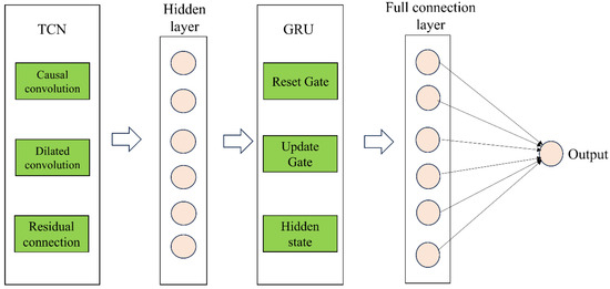
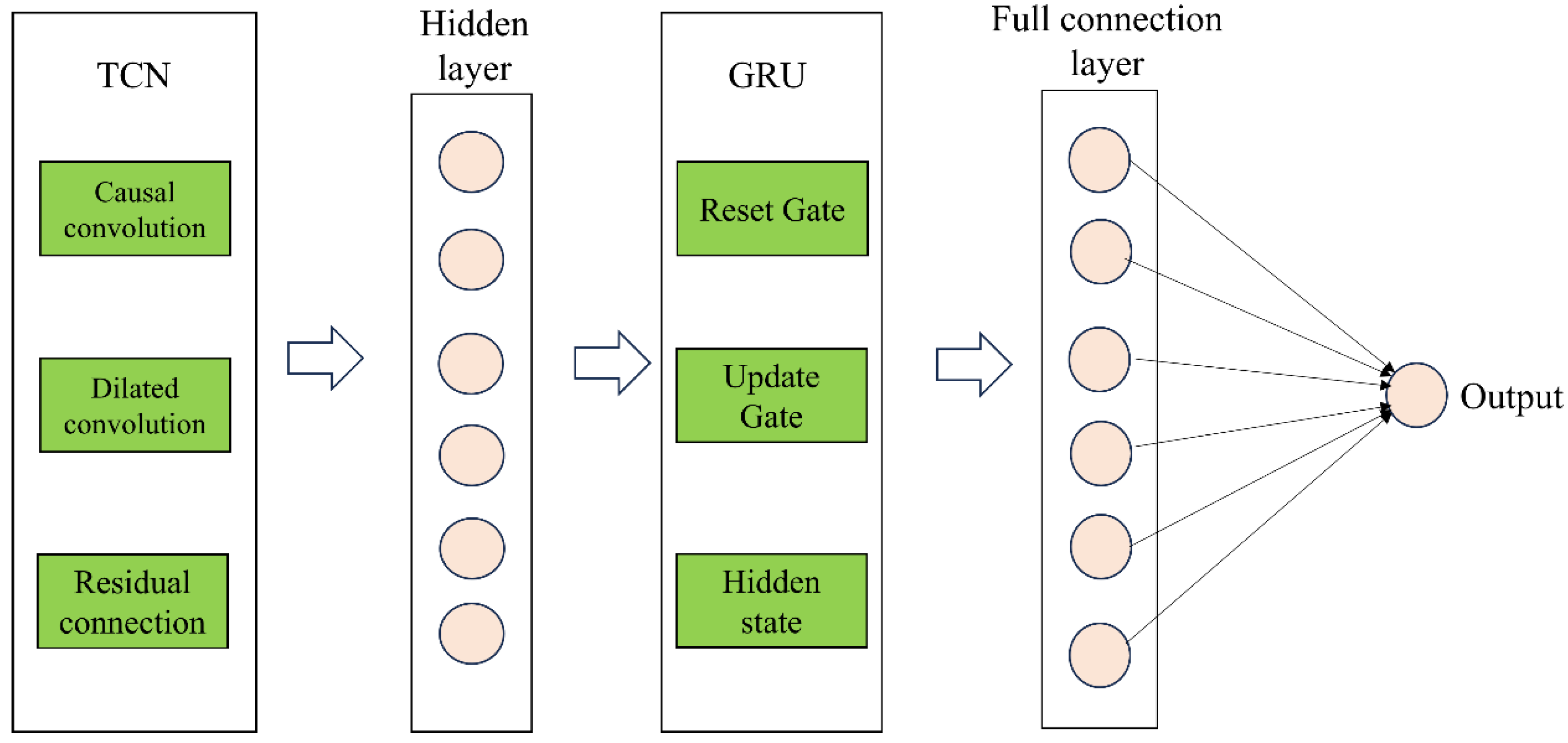
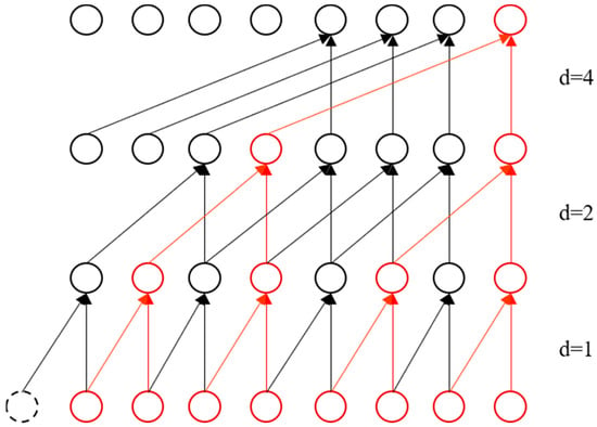
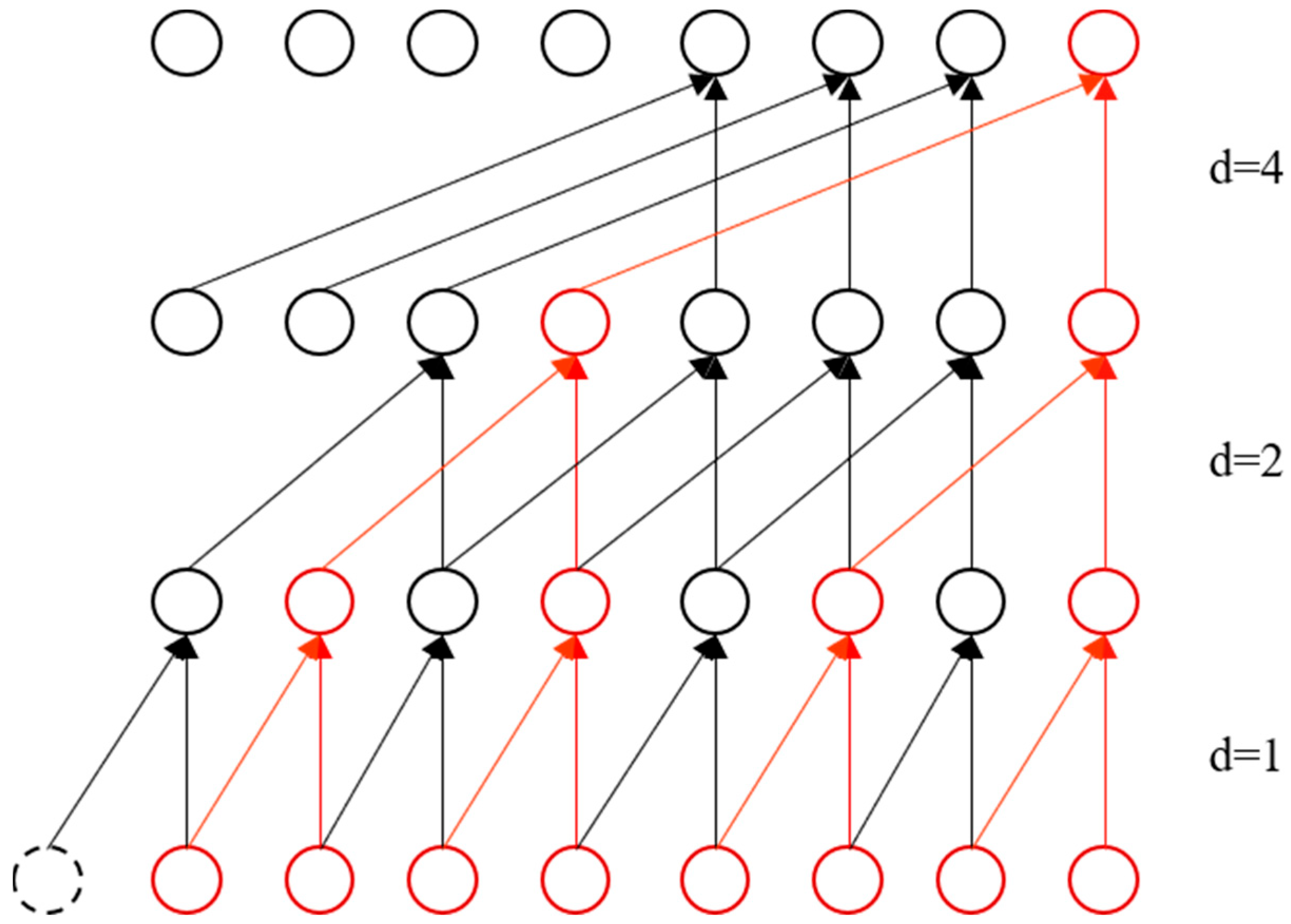
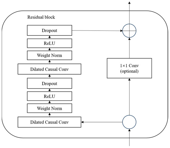
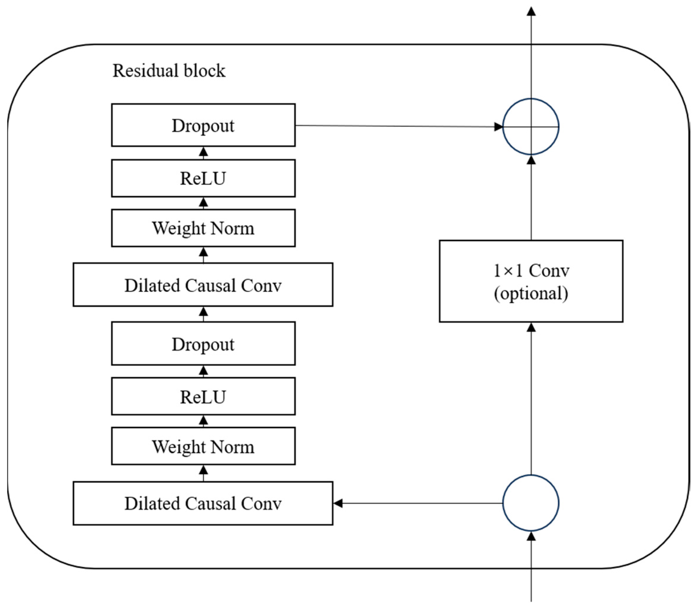
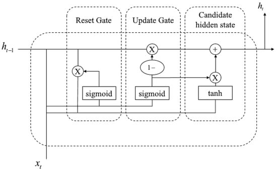
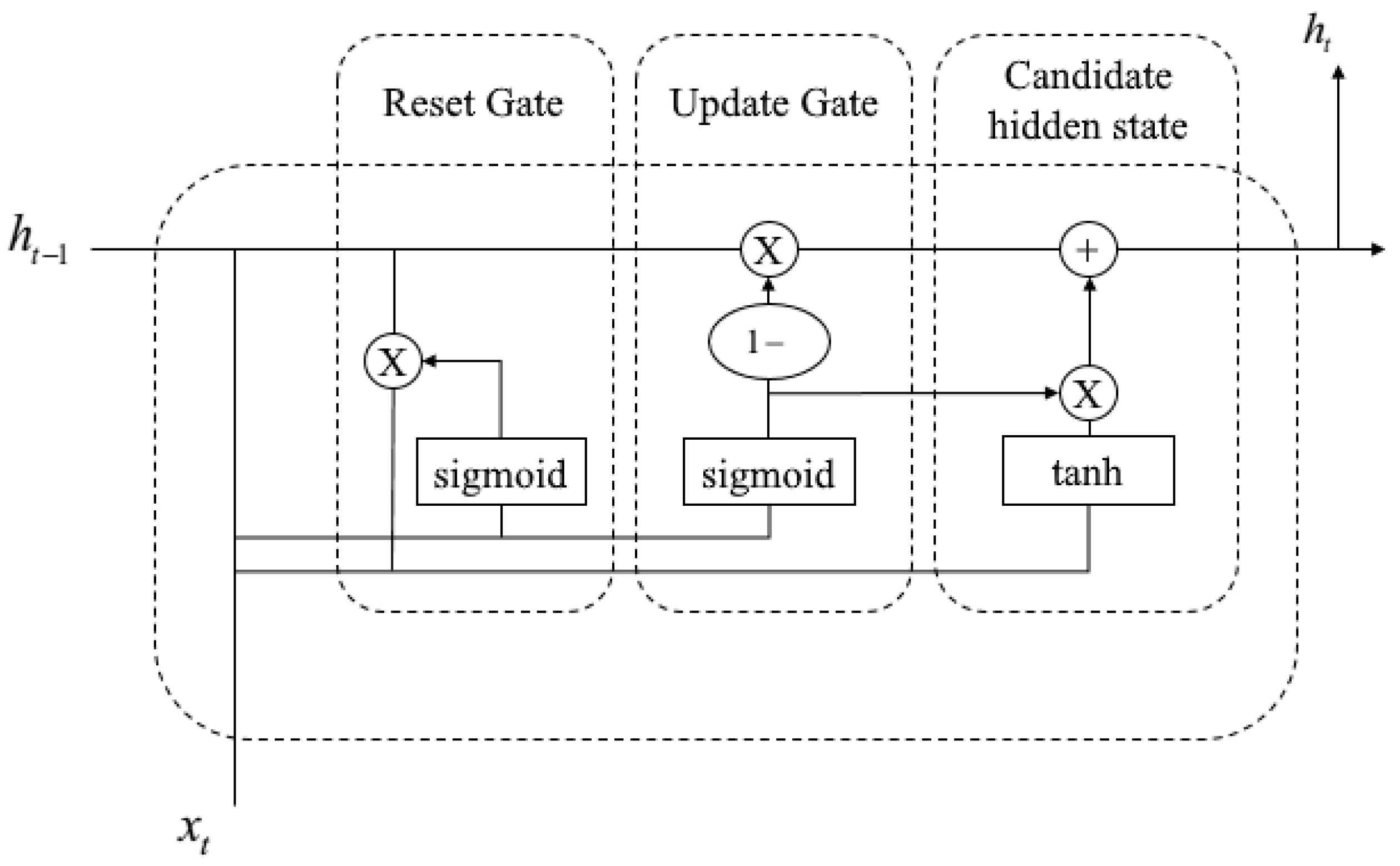
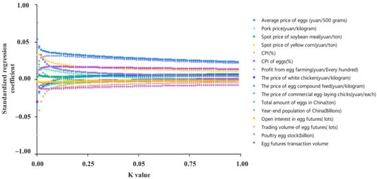
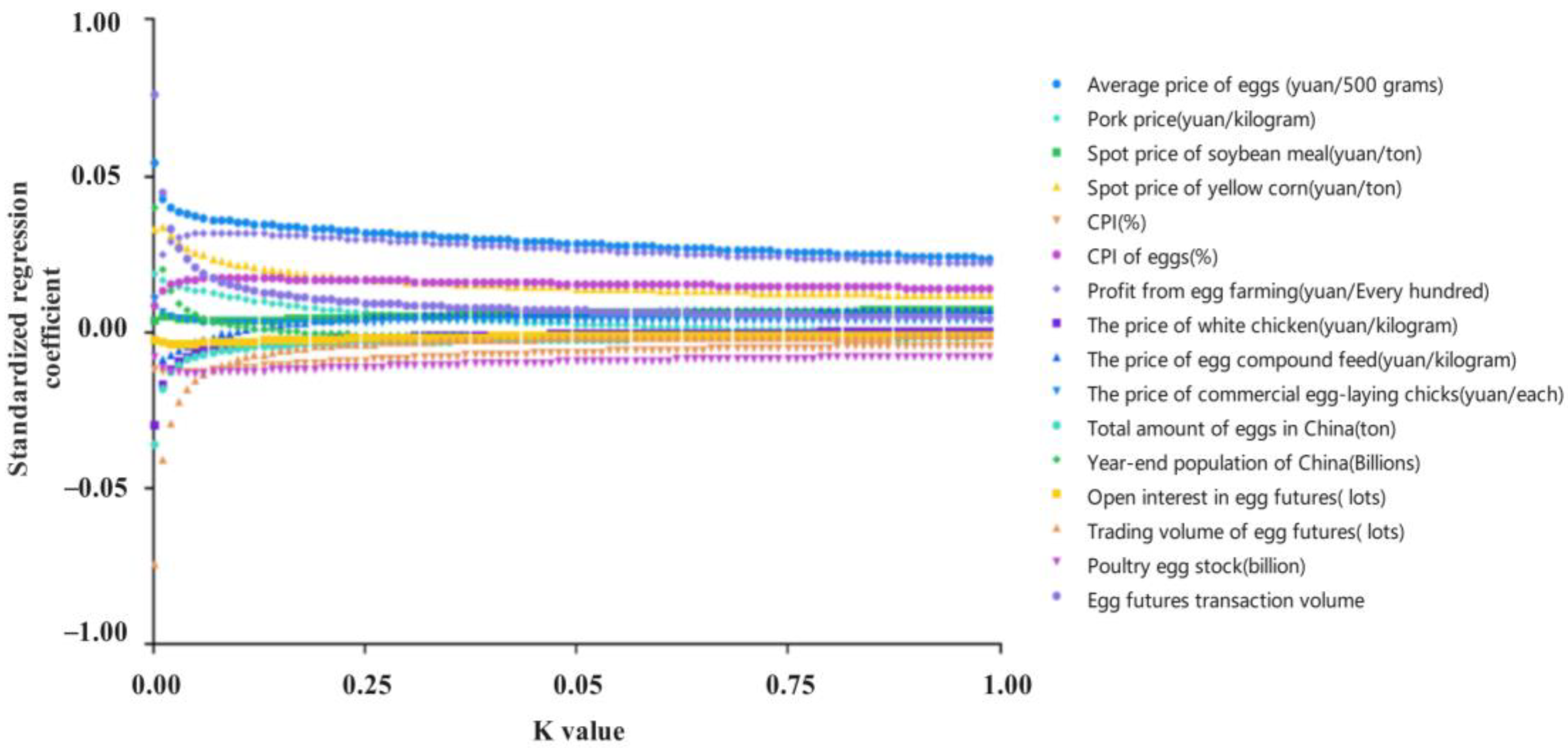
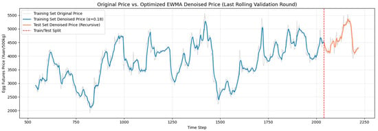
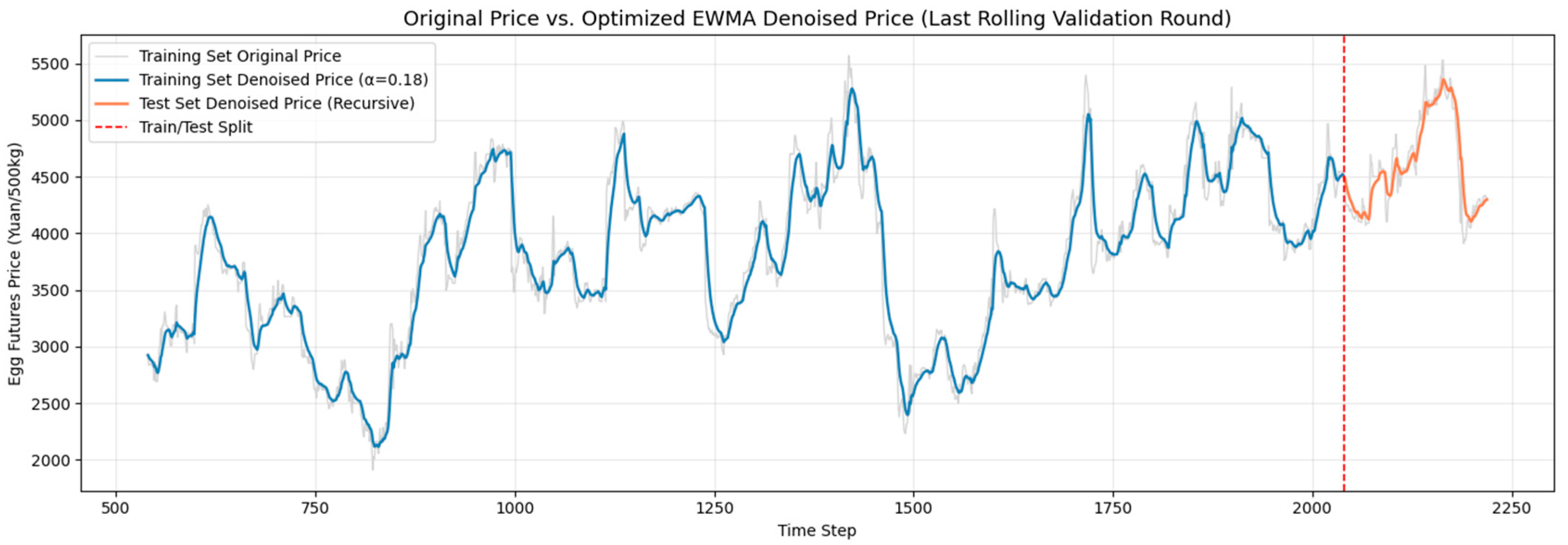
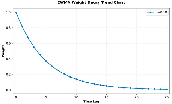
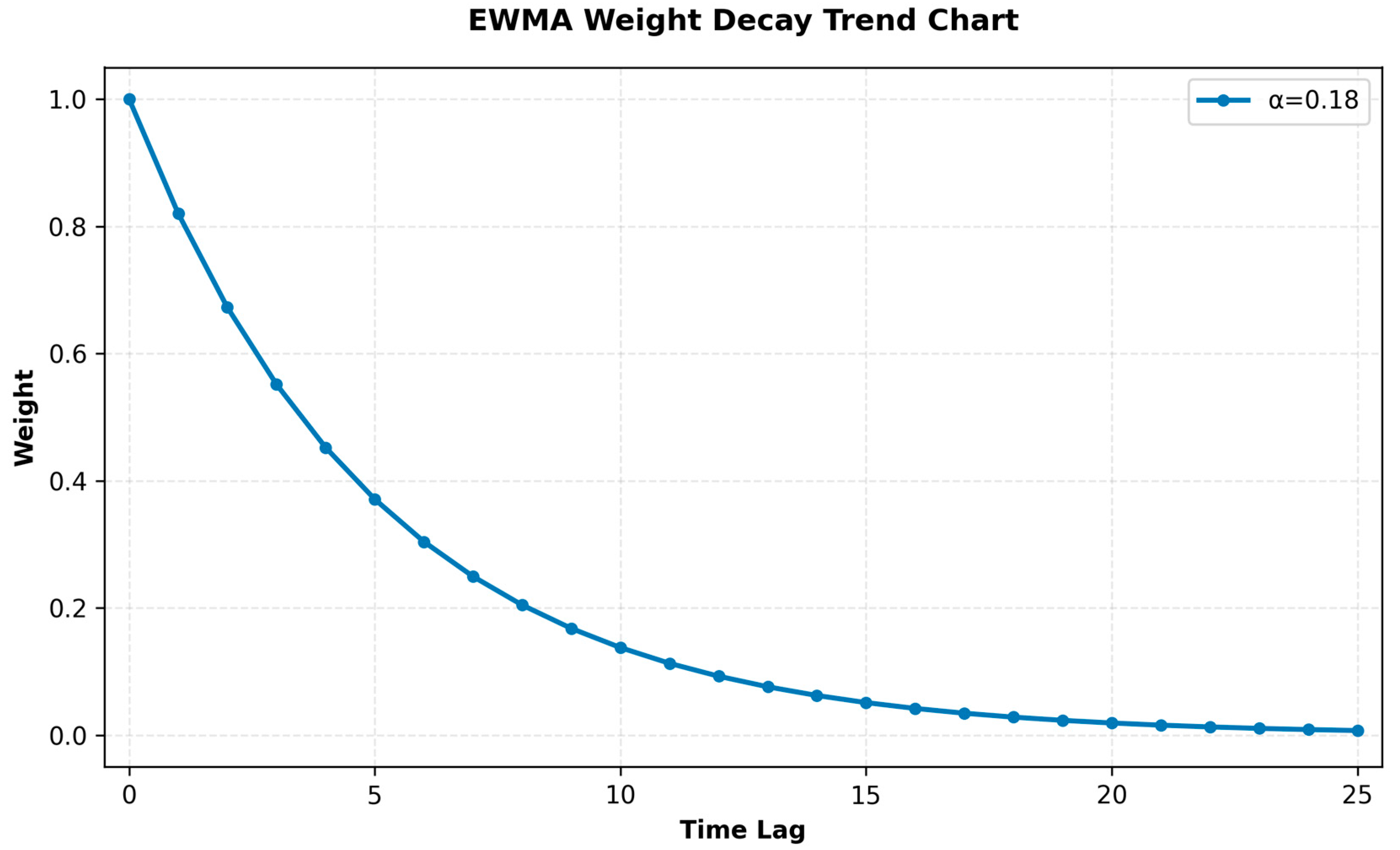
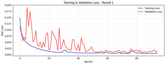
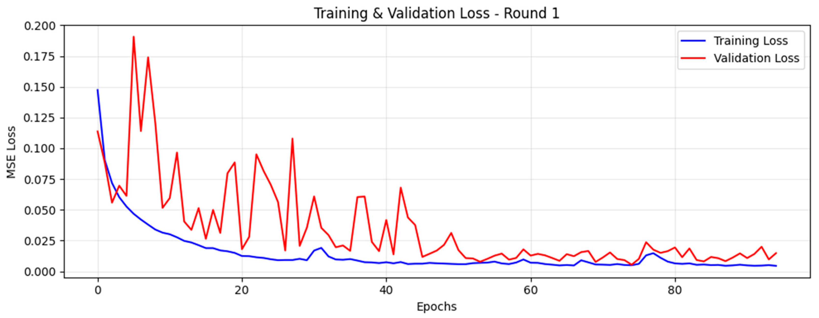
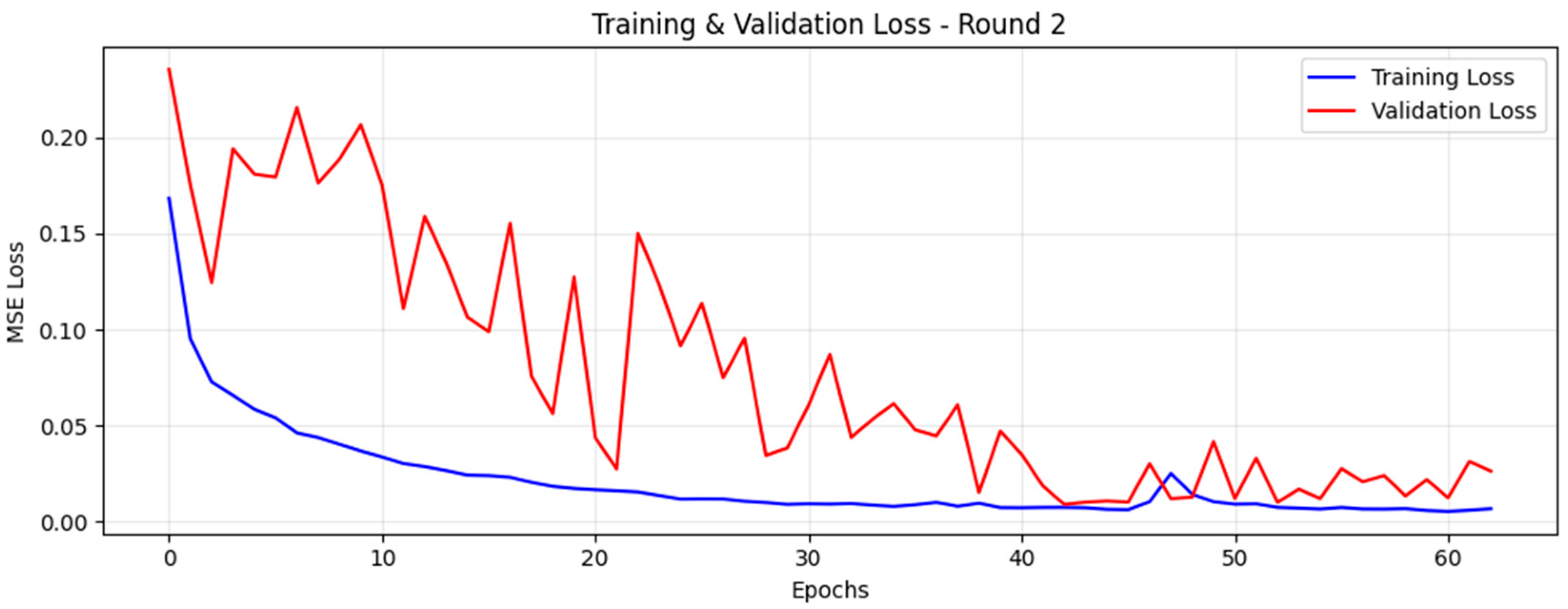
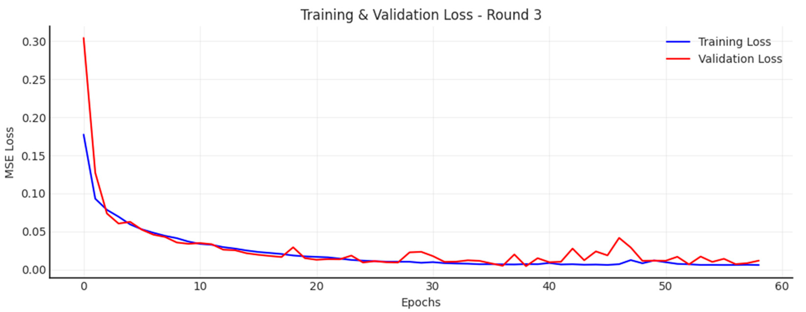
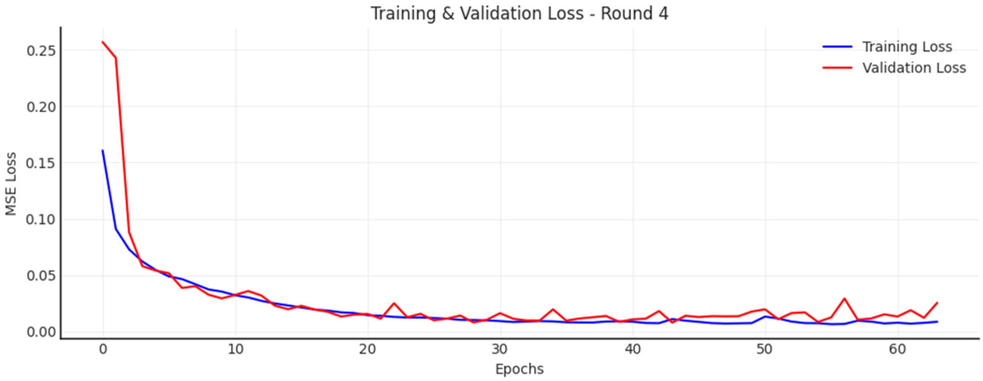
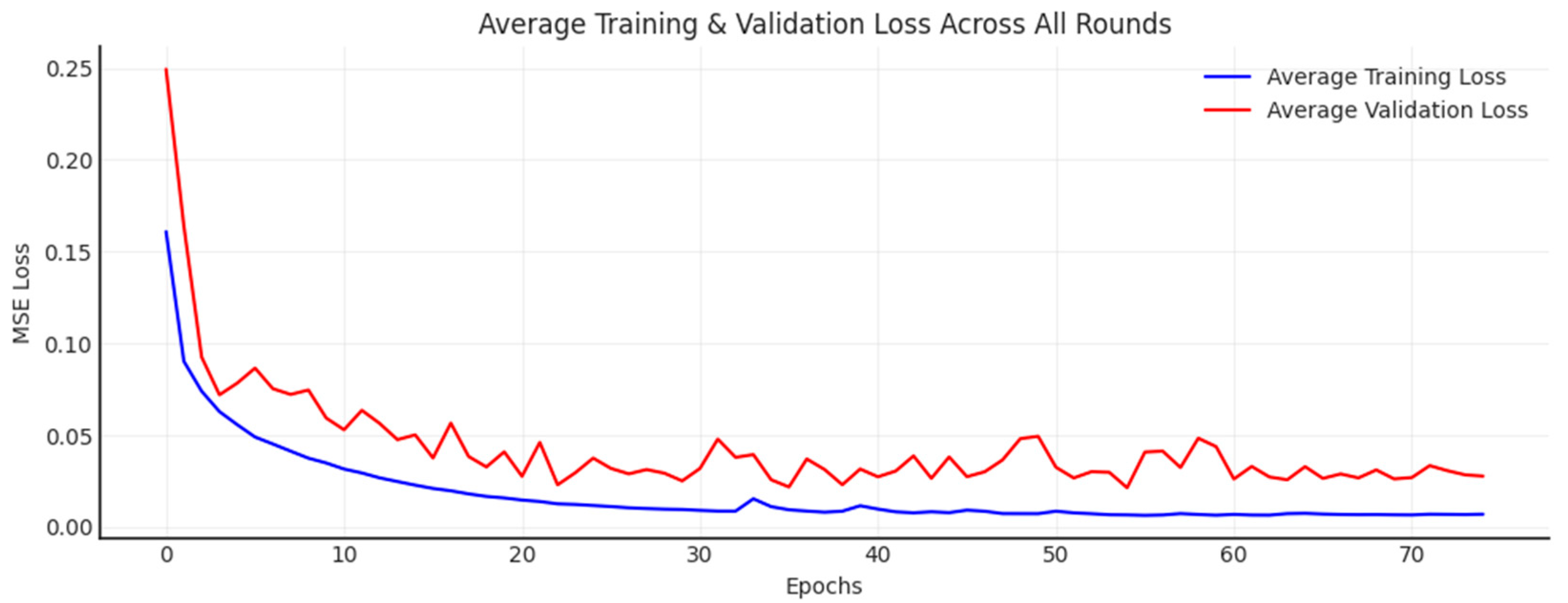
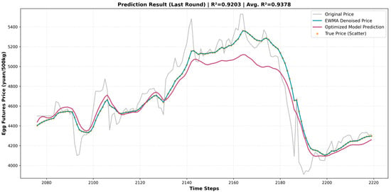
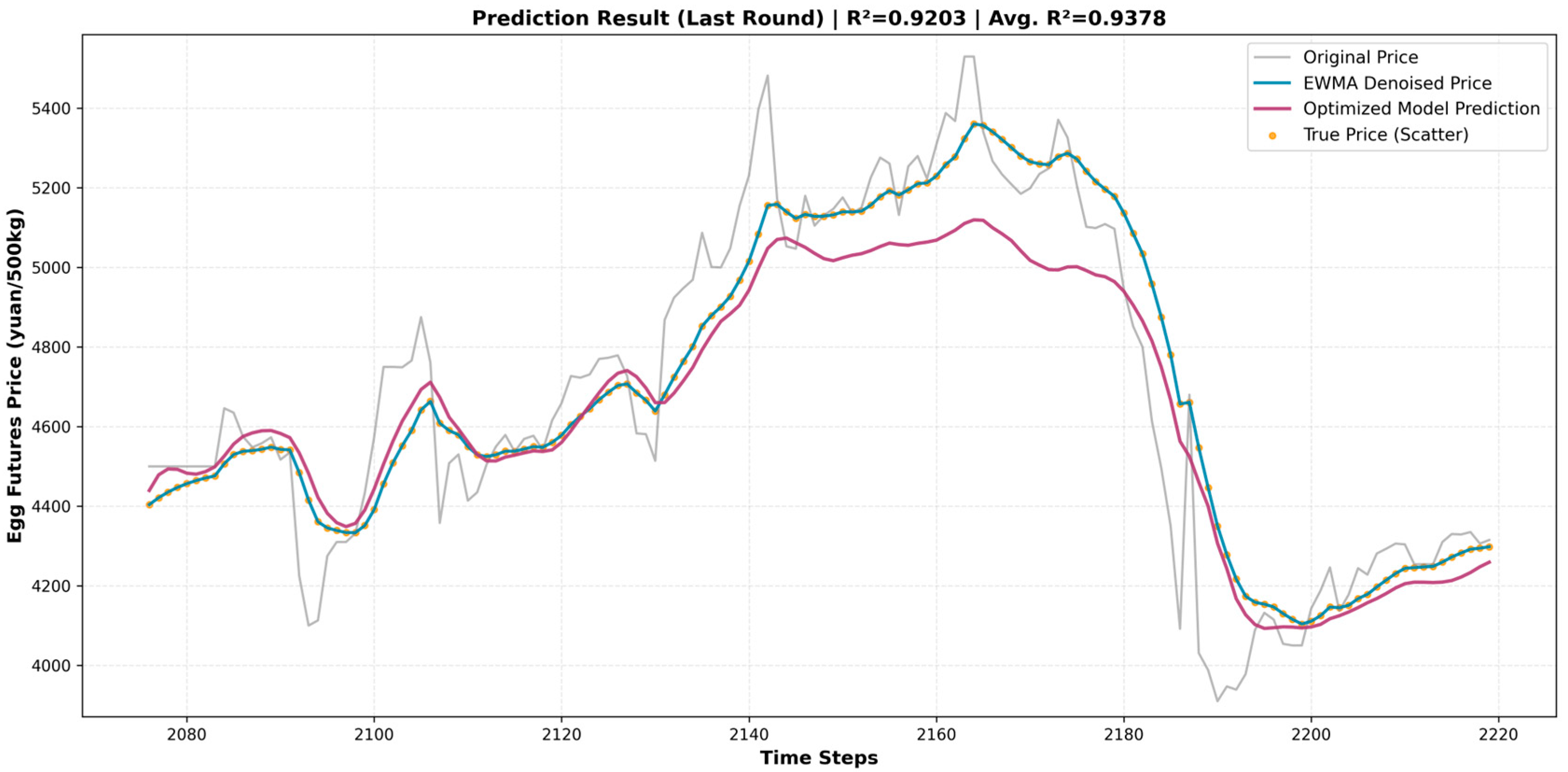
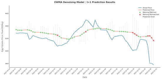
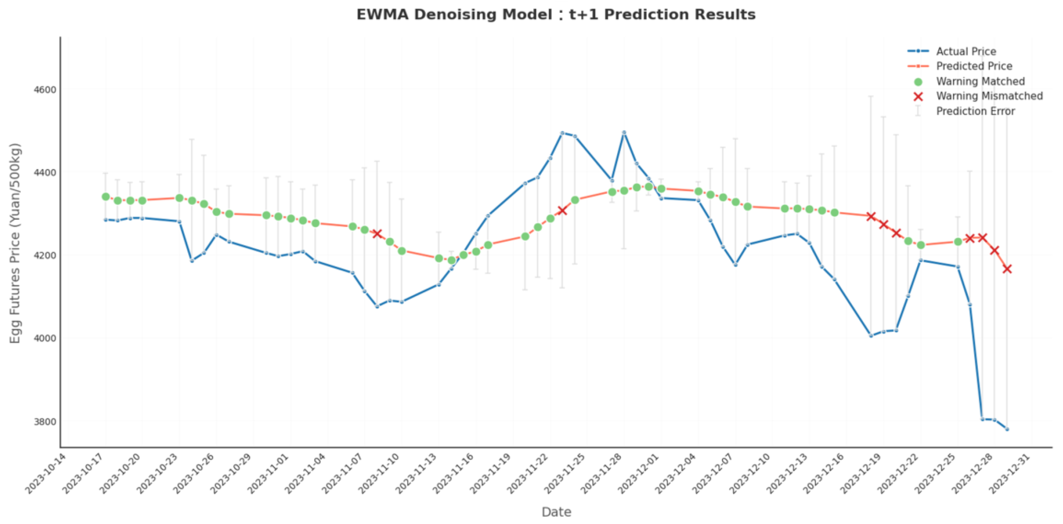
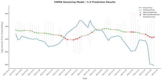
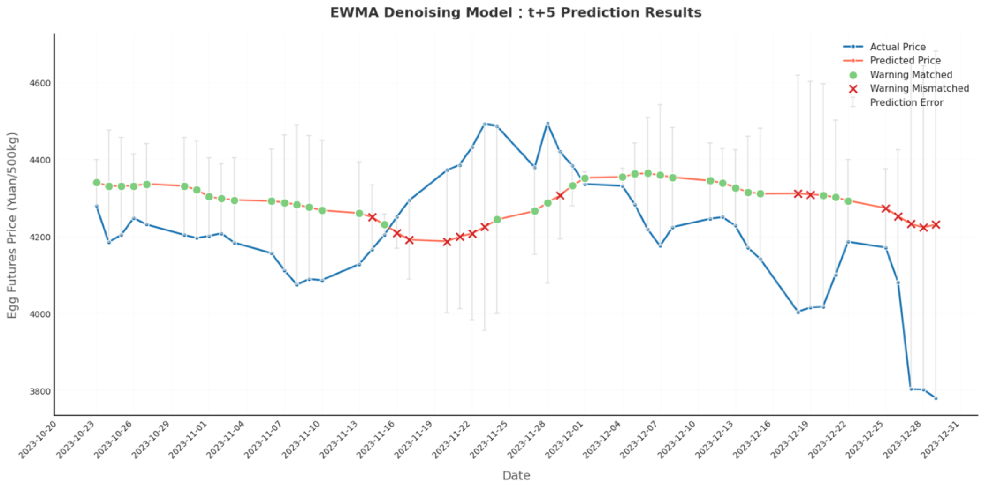
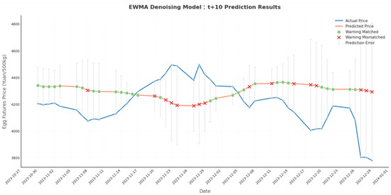
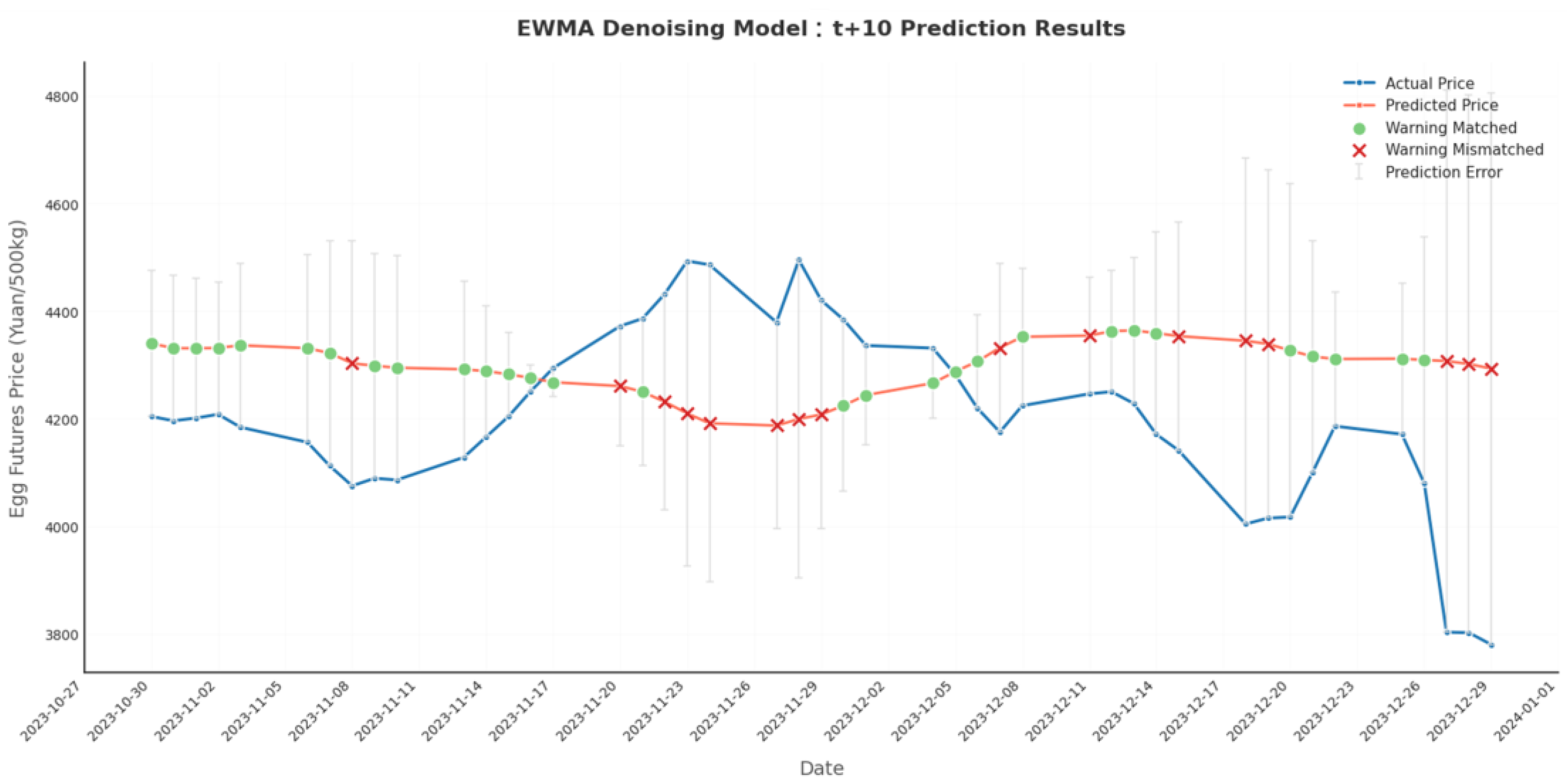
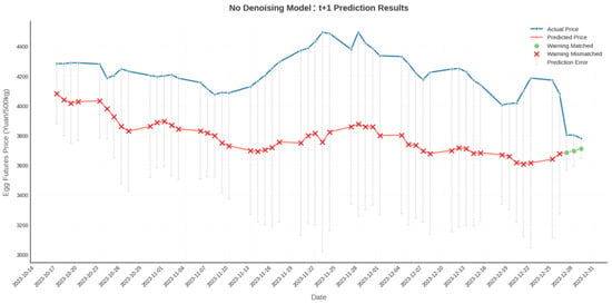
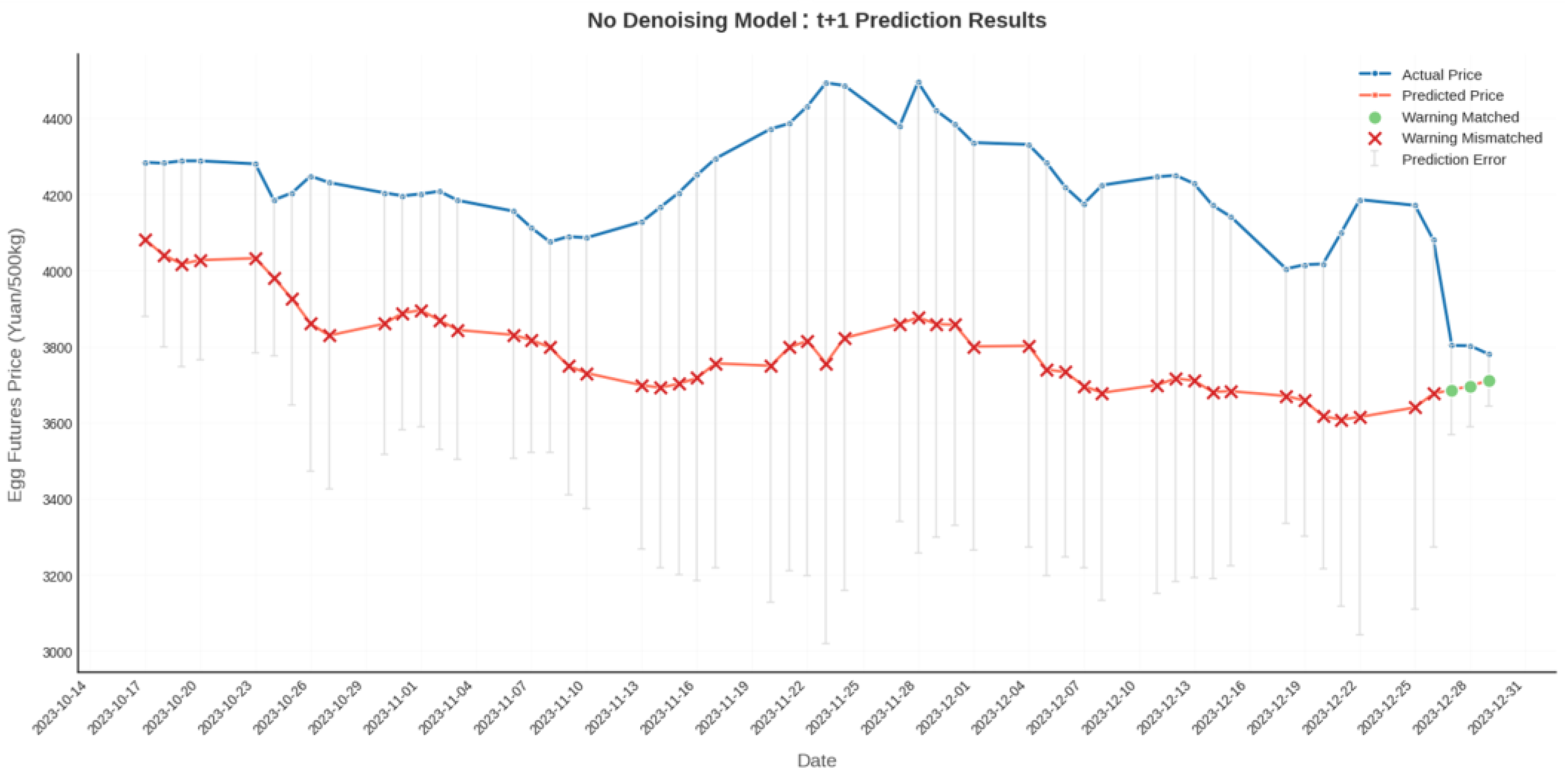
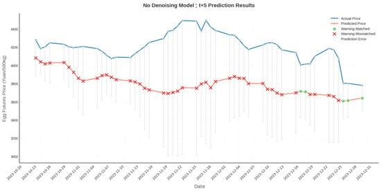
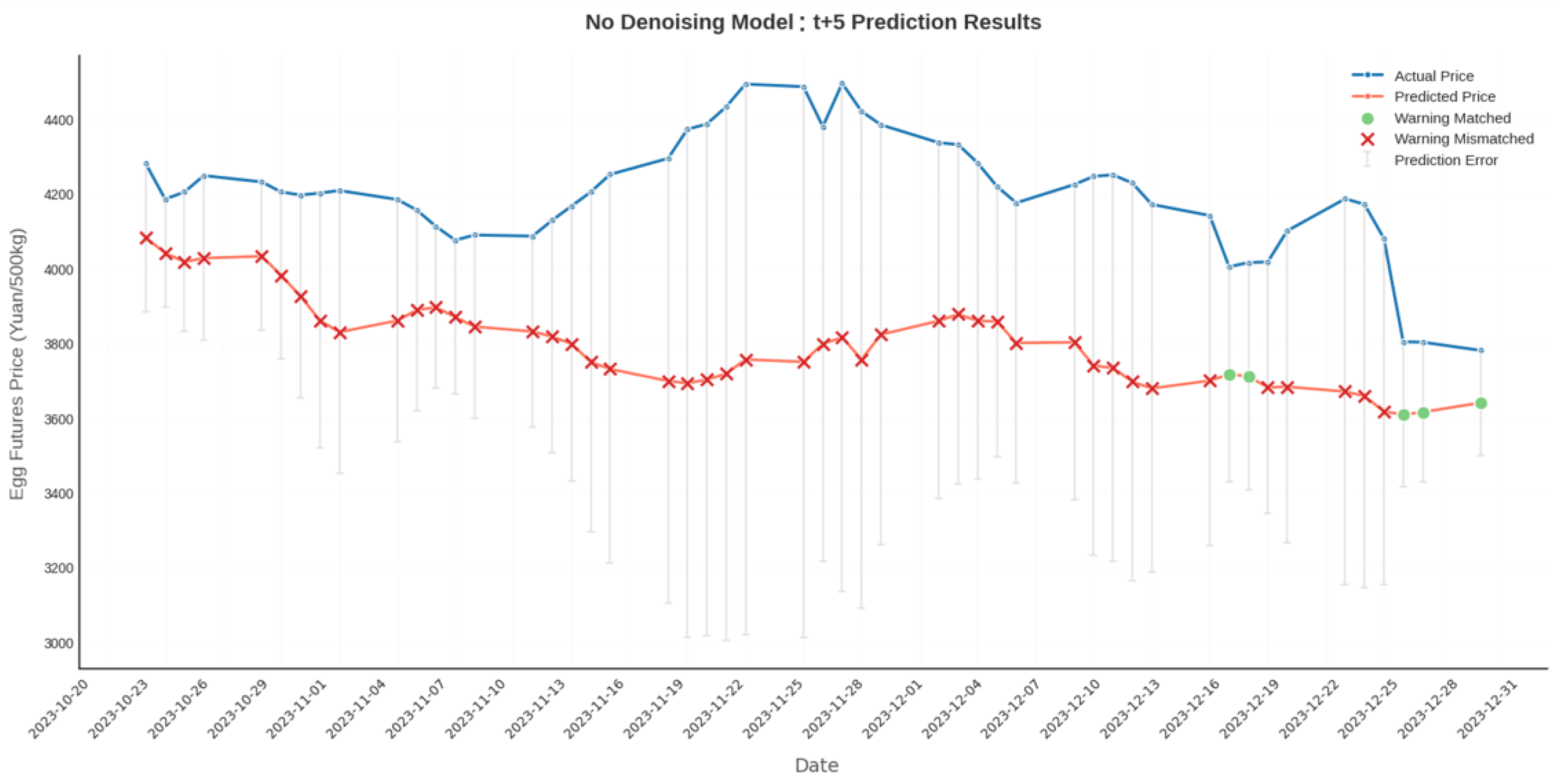
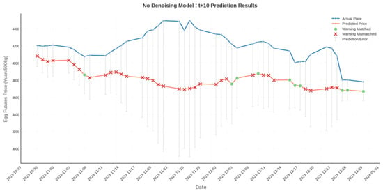
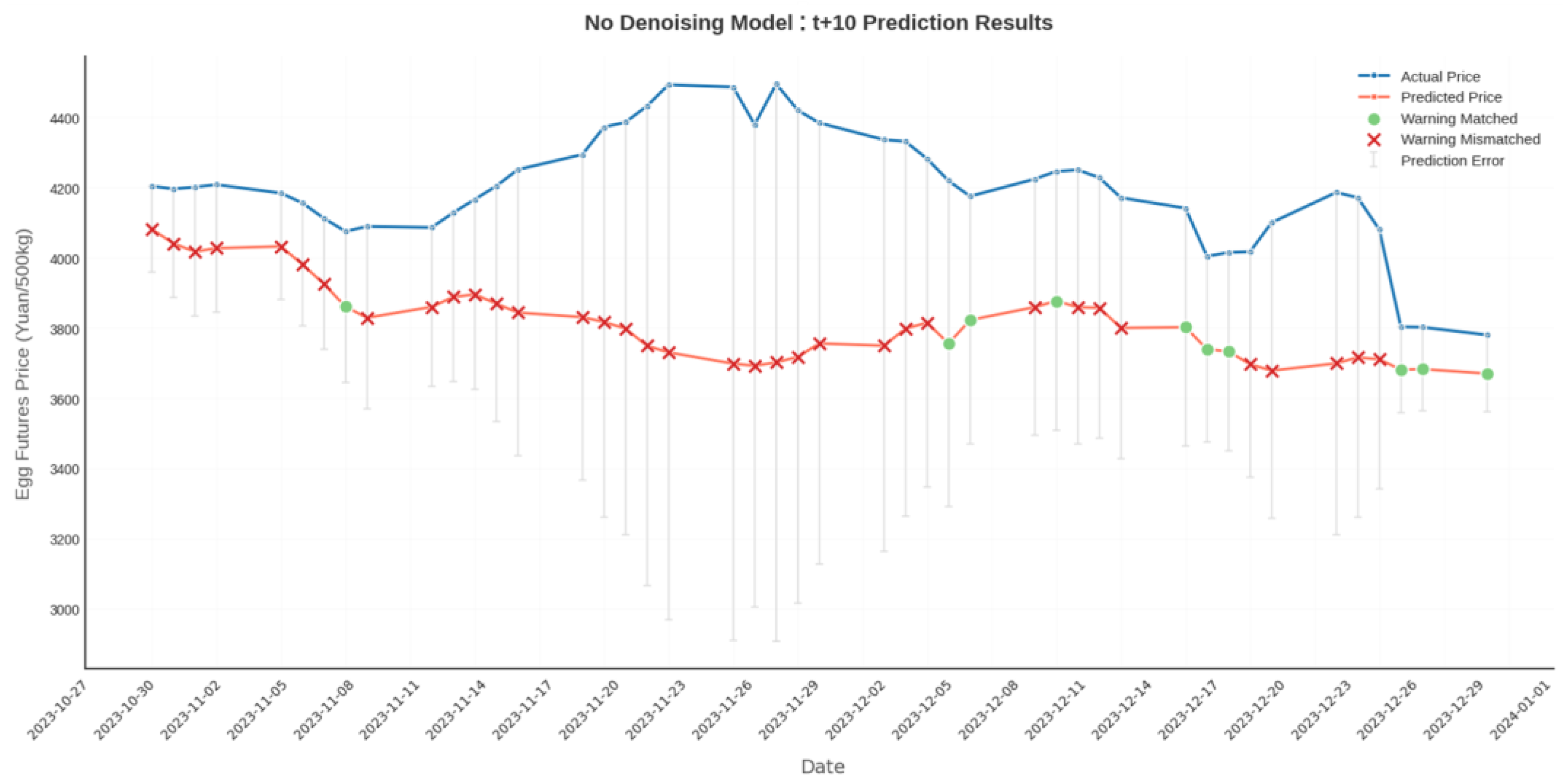

Disclaimer/Publisher’s Note: The statements, opinions and data contained in all publications are solely those of the individual author(s) and contributor(s) and not of MDPI and/or the editor(s). MDPI and/or the editor(s) disclaim responsibility for any injury to people or property resulting from any ideas, methods, instructions or products referred to in the content. |
© 2026 by the authors. Licensee MDPI, Basel, Switzerland. This article is an open access article distributed under the terms and conditions of the Creative Commons Attribution (CC BY) license.