


Abstract
In the context of the rapid advancement of financial technology, the issue of credit card default has become increasingly salient, emerging as one of the crucial risks that financial institutions are eagerly addressing. Traditional credit card default risk prediction models predominantly rely on statistical correlations for feature selection. This approach not only makes it challenging to uncover the genuine causal relationships between variables but also leads to limitations in prediction accuracy and interpretability. To overcome these limitations, this paper presents a novel credit card default risk prediction model that integrates causal feature screening, interaction feature construction, and interpretability enhancement. Initially, by leveraging the information value (IV) and eXtreme gradient boosting (XGBoost), we perform initial feature dimensionality reduction. Subsequently, we introduce the Peter Clark algorithm (PC) augmented with perturbation enhancement and bootstrap sampling to identify a stable set of causal features. Building on this foundation, we proceed to construct higher-order interaction features to bolster the model’s nonlinear modeling capacity. These causal features and their interaction counterparts are then fed into a variety of mainstream machine learning models for training and evaluation purposes. Furthermore, on the basis of the causal feature set identified via the PC algorithm, we construct a causal path diagram. We also incorporate the causal forest double machine learning (causal forest DML) method to estimate the causal effects of features. Additionally, we design a counterfactual explanation mechanism to aid in analyzing the direction and magnitude of the impact of variable interventions on default probability. Empirical tests conducted using four typical credit datasets reveal the following findings: (1) the introduction of causal features generally enhances the model’s performance in terms of the F1 score, area under the curve (AUC), and geometric mean (G-mean). This improvement is especially pronounced in models that are highly reliant on feature quality, such as logistic regression (LR). (2) Causal features offer significant advantages in terms of model interpretability, stability, and compliance, thereby presenting a new research paradigm for credit risk prevention and control in high-risk financial scenarios.
1. Introduction
With the rapid development of financial technology, digital credit has become an important part of global financial services. In China, the development of digital finance has also been rapid, and various digital credit products have been widely used in consumption and payment. However, the rapid development of digital credit has also created many new challenges, especially in the field of credit risk management. Credit default events are constantly emerging, bringing systemic risks and challenges to financial institutions. In fact, in the credit business, credit card default, as one of the most typical risk scenarios, is directly related to the control of nonperforming assets and the profit level of financial institutions. Notably, traditional prediction models generally face the dilemma of insufficient accuracy and lack interpretability when dealing with high-dimensional and nonlinear credit data. Therefore, improving the prediction accuracy of credit card default and the interpretability of models has become a popular and difficult issue in current financial risk research.
In recent years, the application of intelligent algorithms in risk control has continuously increased, which has significantly improved the prediction accuracy of the model. However, these algorithms still have obvious limitations in terms of interpretability and causal reasoning ability, which limits their application value in the formulation of actual credit policies and risk intervention. On the one hand, most mainstream risk prediction methods currently focus on mining the relationship between features and default based on statistical correlation, ignoring the essential difference between correlation and causality. For example, traditional models may identify that “high consumption behavior is highly correlated with default risk”. However, in reality, high consumption is often a manifestation of high-income users who have good repayment ability. Therefore, overreliance on statistical correlation may lead to misjudgment of default risk by the model, weakening the scientific validity and effectiveness of policy intervention. On the other hand, current risk control modeling technology still faces a contradiction between model generalizability and interpretability. Although complex models such as XGBoost and deep neural networks perform well in terms of prediction accuracy, the feature importance indicators output by them have difficulty revealing the causal relationships between features and cannot provide direct guidance for actual risk control strategies. In addition, most traditional models output only the default probability and cannot answer the key question of “how to intervene to reduce default risk”. This limits their application depth in actual credit management scenarios and makes it difficult to meet the regulatory requirements for model interpretability under the Basel III Accord, making compliance with financial institutions’ supervision challenging.
In view of this, this paper focuses on the problem of credit card default risk prediction and aims to integrate causal inference theory with machine learning methods to build a model with higher prediction performance and stronger interpretability. The contributions of this study include the following. First, it overcomes the limitations of traditional modeling, which overly relies on correlation. By using the PC algorithm to identify stable causal features and eliminate pseudo-correlations affected by confounding variables, it transforms from “correlation” to “causality” in modeling and provides a new methodological tool for financial risk management. Second, it innovatively constructs higher-order interactions and nonlinear features on the basis of stable causal variables to improve the model’s generalizability. Third, it combines causal path and effect analysis to transform the model from “prediction” to “interpretation and intervention”, providing a risk intervention chain that meets regulatory requirements and avoids algorithmic compliance disputes. Fourth, multiple public credit datasets are tested, and the results verify the advantages of combining causal features with the LR algorithm.
The rest of this paper is organized as follows: Section 2 is the literature review; Section 3 introduces the theoretical basis and modeling process of the study; Section 4 elaborates on the algorithm comparison experiments and results and analyzes the causal features in terms of path and effect; and Section 5 is the summary of the entire paper and the outlook for future work.
2. Literature Review
This section systematically reviews the current research on credit default prediction. It analyzes the literature from two aspects: credit risk identification and the integration of causal inference with machine learning. This provides a solid theoretical foundation for subsequent research.
2.1. Credit Risk Identification
2.1.1. Traditional Statistical Models
Credit risk identification has long been a central problem in financial risk management. Early studies primarily relied on statistical modeling techniques. For example, Sohn et al. [1] introduced a fuzzy logistic regression model that incorporated fuzzy sets to address uncertainty in qualitative indicators. However, the approach retained the linear assumptions of logistic regression and therefore failed to capture complex nonlinear relationships among variables.
Similarly, Chang et al. [2] combined survival analysis with logistic regression to model dynamic mechanisms through survival functions. Yet, the logistic component remained limited in representing nonlinear interactions among multidimensional features. Zhou et al. [3] further demonstrated that linear support vector machines neglect feature interactions in long-term default prediction, resulting in degraded accuracy.
Overall, traditional statistical models rely primarily on correlation-based variable selection rather than causal mechanisms. This limits their ability to model nonlinearities and higher-order interactions, thereby constraining predictive performance.
2.1.2. Machine Learning—Based Models
In recent years, machine learning techniques—such as random forests (RF), XGBoost, and deep neural networks (DNNs)—have been widely adopted in financial risk control and have demonstrated strong performance in credit default prediction. Zhang et al. [4] developed a multi-model machine learning framework for loan default prediction, validating its practical value in business process management. Dichev et al. [5] further showed that machine learning exhibits strong capabilities in financial transaction risk assessment and decision support.
Despite these advances, two major challenges remain.
- (1)
- Limited Interpretability in High-Stakes Scenarios.
Ensemble methods often improve predictive accuracy but sacrifice interpretability. For instance, Gao et al. [6] proposed a LightGBM-based hybrid model that achieved 84.36% accuracy on the Renrendai platform; however, the split rules in gradient boosting trees lack transparent economic interpretation. Zhang et al. [7] introduced TE-ResNet, which employs a Transformer encoder to automatically extract associations among high-dimensional sparse features and improved AUC by 2.85% on the Tianchi dataset. Nevertheless, attention weights are difficult to map to actionable financial risk semantics. Yan et al. [8] developed WIGNN to enhance interpretability through explicit weight computation and modular design, yet the reinforcement learning strategy and internal graph neural network representations remain largely opaque.
- (2)
- Feature Sensitivity and Robustness Concerns.
Machine learning models depend heavily on feature engineering and are vulnerable to noise and multicollinearity. Chi et al. [9] proposed a stacking ensemble model with Lasso-logistic feature selection; however, the process is sensitive to regularization strength and may exclude critical variables. Chugh et al. [10] combined CBLOF with isolation forest and applied PCA-based preprocessing to address class imbalance, yet noise and multicollinearity in high-dimensional credit card datasets continued to affect stability. Chi et al. [11] proposed DeepFM-KG, integrating knowledge graph embeddings with deep factorization machines to fuse multi-source features and improve predictive accuracy. However, the model relies heavily on high-dimensional sparse features and embedding representations; without causal filtering or redundancy reduction mechanisms, it remains susceptible to noise and multicollinearity.
2.1.3. Modeling with Interpretability Mechanisms
To address the limitations above, recent work has incorporated explicit interpretability mechanisms into model design. For example, Kong et al. [12] proposed CFTNet, which integrates counterfactual generation and reinforcement learning to formulate the prediction process as a Markov decision process. By analyzing model behavior from a causal perspective, the approach enhances interpretability. Zandi et al. [13] introduced temporal attention to assign differentiated weights across time steps, improving interpretability along the temporal dimension, and employed graph attention networks (GATs) to capture relational importance among nodes for local structural explanations. Sun et al. [14] and Kagaba et al. [15] applied post hoc explanation tools such as SHAP and LIME to support global feature attribution and local prediction analysis. Similarly, Arias-Serna M.A. et al. [16] combined interpretable machine learning models with risk assessment pipelines, improving transparency while preserving predictive performance. These efforts reflect a broader shift toward integrating explanation directly into the modeling process.
Despite these advances, several limitations remain. First, most approaches rely on post hoc explanations and do not penetrate deeply into learned representations. Second, different explanation techniques may yield inconsistent feature rankings (e.g., SHAP vs. LIME), undermining reliability.
Integrating causal inference directly into the training process offers a principled alternative. By coupling causal feature identification with model optimization, it becomes possible to improve interpretability, robustness, and transferability simultaneously. This paradigm shift—from correlation-based modeling to mechanism-oriented causal modeling—can enhance transparency and operational reliability in high-stakes financial applications while maintaining predictive accuracy. Table 1 summarizes existing approaches to credit risk identification.
Table 1.
Existing credit risk identification methods.
2.2. Integration of Causal Inference and Machine Learning
The integration of causal inference and machine learning has emerged as a prominent direction in intelligent risk modeling. Causal inference provides a principled framework for identifying underlying mechanisms among variables. In particular, Judea Pearl [17] introduced the three-level hierarchy of causation—association, intervention, and counterfactual—which formalizes questions such as why a variable affects an outcome and whether modifying a feature can reduce default probability.
Existing studies that combine causal inference with machine learning can be broadly categorized into two paradigms.
- (1)
- Causal Validation of Machine Learning—Identified Features
This line of work first applies machine learning to identify predictive features, and then uses causal inference to validate their causal effects, thereby improving credibility and interpretability.
For example, Bakir et al. [18] proposed a “triple validation” framework: a deep neural network predicts non-performing loan ratios, random forests rank feature importance, and DoWhy is used to validate the causal effects of foreign direct investment (FDI) and policy interest rates. Peng et al. [19] employed ensemble learning to predict default risk and then applied DoWhy to assess the causal impact of state ownership, revealing indirect risks associated with implicit guarantees.
Ying et al. [20] used XGBoost for churn prediction, SHAP for feature attribution, and the R-learner to estimate causal effects. In related work, they combined water quality prediction with causal analysis: random forests and SHAP identified key predictors, and causal graphs were used to verify the causal impact of discharge outlets on nitrogen and phosphorus pollution.
Similarly, Noh et al. [21] predicted diabetes risk using catboost-1.1.1 and XGBoost 2.0, constructed a causal network via LiNGAM, and quantified intervention effects with DoWhy 0.11.1., forming an integrated pipeline of prediction, causal discovery, and intervention evaluation for personalized health management.
- (2)
- Machine Learning over Causally Selected Features
The second paradigm reverses the order: causal inference is first used to identify key variables and eliminate spurious correlations, after which machine learning models are trained on the causally filtered feature set to enhance interpretability and generalization.
Song et al. [22] applied causal inference to preselect critical variables, then used CatBoost to predict BPA degradation efficiency, and validated positive causal effects using DoWhy. Founta et al. [23] proposed a closed-loop workflow of causal feature selection, model training, and SHAP-based interpretation. Using the SES algorithm, they extracted causally relevant gene subsets associated with ALS from high-dimensional genomic data, followed by modeling with XGBoost and random forests. Table 2 summarizes representative approaches that integrate causal inference and machine learning.
Table 2.
Current State of Research on the Integration of Causal Inference and Machine Learning.
Compared with the first category of “machine learning-based and causal inference-assisted” methods, the second category of “causal inference-based and machine learning as a modeling tool” methods has stronger interpretability. This is especially true in the financial risk control field, where variable relationships are highly sensitive and a strict interpretation of results is needed. In key risk judgment tasks such as credit scoring and loan default, accurately identifying the causal variables that truly affect default behavior and excluding the interference of confounding variables and pseudo-correlated variables are key to improving model credibility and decision quality. Therefore, causal-driven feature extraction methods have great application potential in risk control systems. However, the application of such methods in credit card default risk prediction is relatively rare at present. Existing research has focused mostly on the fields of medical care, the environment, and gene screening and has not yet formed a closed-loop process of “causal feature screening-machine learning modeling-causal interpretation”, which is systematically applicable to financial scenarios.
On this basis, this paper proposes a credit default risk prediction model that integrates causal feature selection, interaction feature construction, and interpretability. First, on the basis of the PC algorithm, variables that have a stable causal relationship with default are identified. Second, on the basis of the screened causal features, further causal feature engineering and interaction feature mining are carried out to enhance the model’s ability to model complex causal mechanisms. The causal features are subsequently input into various machine learning models for modeling and prediction. The prediction performance of different models under the support of causal features is compared to verify the universality and robustness of the method. Finally, the causal path and its causal effects obtained via the PC algorithm are analyzed to explain which causal variables have a significant impact on default and the extent of their impact, clarify the prediction mechanism and reveal the direction of action and intervention potential of key causal variables. Through the construction of this model, not only can the interference of pseudo-correlated variables be effectively eliminated and its stability enhanced, but it is also more conducive to enhancing the operability and interpretability of the model in actual risk control decision-making, providing theoretical support and a decision-making basis for building a transparent, fair, and reliable credit scoring system.
3. Research Methodology
This section delineates the credit card default risk prediction modeling framework proposed in this study, systematically presenting the core theoretical methodologies and modeling procedures. We first expound the theoretical foundations of model construction from four perspectives: causal feature extraction, interaction feature construction, causal effect estimation, and counterfactual reasoning. We subsequently elucidate the role of each stage within the integrated modeling process to establish a theoretical foundation for subsequent empirical analysis.
3.1. Theoretical Basis
3.1.1. Causal Feature Extraction
The PC algorithm, a constraint-based causal structure learning method, infers directed acyclic graphs (DAGs) among variables from observational data. Within causal modeling, this algorithm identifies features constituting direct causal parent nodes of the target variable, thereby enabling causal feature selection. Its core methodology iteratively eliminates improbable edges through conditional independence tests before orienting the remaining edges to derive a plausible DAG. To enhance feature stability, we implement a multiscale perturbation approach that combines Gaussian noise, salt-and-pepper noise (SPN), and masking techniques for randomized sample perturbation. Concurrently, we employ bootstrap sampling, wherein 80% of the subsamples are randomly drawn from the original data to simulate data uncertainty and distributional drift. This dual strategy evaluates causal edge stability across perturbations. Building upon multiple perturbation-augmented causal graphs, we compute the frequency of each feature appearing as a target variable’s causal parent node. The ten highest-frequency features constitute the final causal feature set (retaining all if fewer than ten stable features exist), ensuring stable causal effects under data perturbations while mitigating spurious correlations. The procedure comprises five steps:
- (1)
- Feature Subset Standardization
Given dataset D = {X1,X2,…,Xp,Y} where Yϵ{0,1} is the target variable and X = {X1,X2,…,XP} denotes the input features, we standardize the features as:
where μj and σj represent feature wise means and standard deviations, respectively, ensuring conditional independence test validity.
- (2)
- Multiperturbation Robustness Enhancement
To fortify causal graph stability under limited samples, we generate perturbed sample sets D(b) via:
where N(0,σ2) denotes Gaussian noise, SaltAndPeppter introduces extreme-value perturbations, and MaskNoise simulates feature missingness through random masking and permutation, collectively testing feature selection robustness.
To ensure that perturbations remain consistent with the statistical properties of financial data, we model three types of noise as approximations of common observational error mechanisms in credit datasets:
Gaussian noise simulates measurement error and statistical fluctuation in continuous financial variables introduced during data collection and normalization (e.g., approximately normal deviations in income or debt-to-income ratios).
Salt-and-pepper noise models extreme values and anomalous records, approximating batch import errors, abnormal transaction entries, or boundary distortions induced by discretization.
Masking perturbations represent missingness and incomplete information, which are prevalent in credit data due to reporting omissions, delayed updates, or unobservable variables.
These three perturbation types correspond to measurement error, outlier shocks, and missing-data mechanisms—three primary sources of bias in real-world data generation. We jointly inject these perturbations under repeated resampling and apply stability selection, retaining only those causal parent nodes that consistently appear across heterogeneous error conditions. This procedure enhances the robustness of causal structure learning against data imperfections. Importantly, the perturbation mechanisms are not intended to replicate the true data-generating process. Rather, they approximate common observational biases and serve as a robustness filtering strategy, not as a substitute for structural identification.
- (3)
- Causal graph learning via the PC algorithm
For each perturbed sample D(b) ϵ Rn×(p+1), the PC algorithm is used to learn its causal structure graph. This algorithm assumes that the data satisfy the Markov condition and stability assumption, progressively eliminating edges through conditional independence tests. Fisher’s Z conditional independence test function is used:
The Z statistic is calculated as follows:
where rij.s is the partial correlation coefficient under the conditioning set S. If p-value(Z) > α, it is concluded that , and the corresponding edge is removed from the graph.
- (4)
- Direct cause extraction from the causal graph
Let the directed acyclic graph learned under the b perturbation be G(b). All the features corresponding to the edges pointing to the target variable Y are extracted:
- (5)
- Voting Fusion and Feature Ranking
Count the frequency fi of each feature appearing as a causal parent node of Y over B samplings. The final score is defined as:
The top 10 features with the highest scores form the stable causal feature set, as shown in Equation (7):
This method surpasses correlation-based feature selection by eliminating noncausal correlates of Y. Crucially, it addresses multicollinearity-induced false positives inherent in traditional approaches. By leveraging conditional independence tests, the PC algorithm hierarchically removes chain correlations mediated by covariates or confounders, retaining only parent nodes with direct causal relationships to Y. The selective extraction of features with directed edges to Y structurally suppresses multicollinearity bias while ensuring causal interpretability. The complete algorithmic workflow is formalized in Table 3.
Table 3.
Stable Causal Feature Selection Algorithm Flow.
It is important to note that the structural discovery capability of the PC algorithm relies on core assumptions such as causal sufficiency and faithfulness. In real-world credit datasets, these assumptions may hold only approximately. To mitigate the risk of structural misidentification, we incorporate perturbation-based augmentation, stability selection, and multi-stage causal validation. The associated limitations and their implications are discussed in detail in subsequent sections.
3.1.2. Interaction Feature Construction
To enhance the model’s ability to express nonlinear and higher-order relationships between features, this paper designs an interaction feature construction and screening module based on causal feature selection. It prioritizes interaction features that have a stable causal relationship with the target variable, supporting interactions between categorical and numerical features, as shown in Table 4.
Table 4.
Interaction feature types.
3.1.3. Causal Effect Estimation
Following causal path identification and effective path screening, we employ the DoWhy framework with the causal forest double machine learning (CausalForestDML) method to quantify treatment effects on default outcomes. CausalForestDML combines causal forests with double machine learning (DML) to estimate heterogeneous treatment effects, making it suitable for modeling conditional average treatment effects (CATEs) under high-dimensional confounding. The method implements a backdoor adjustment strategy by conditioning on covariate set X to block confounding paths between treatment T and outcome Y, producing bias-corrected causal estimates. The two-stage estimation procedure involves the following steps:
First, the conditional expectation of the treatment variable is shown in Equation (8):
The second is the conditional expectation of the outcome variable, as shown in Equation (9):
The CATE for each unit is subsequently estimated via residual regression:
Finally, the average treatment effect (ATE) is obtained via CATE, which is calculated via Equation (11):
This approach leverages random forests’ ability to model high-dimensional nonlinear relationships, making it particularly suitable for financial data characterized by complex feature interactions.
3.1.4. Counterfactual Simulation Verification Based on ATE
Let Yi(1) and Yi(0) denote potential outcomes under treatment and control conditions for unit i with covariates Xi. ATE represents the population-level causal effect:
Within the backdoor adjustment framework, ATE is estimated as:
For continuous treatments, ATE represents the expected outcome change per unit treatment increase:
3.1.5. Counterfactual Intervention Simulation Based on the Logistic Regression Prediction Model
This method involves constructing an interpretable logistic regression prediction model to simulate the impact of counterfactual interventions on a single treatment variable on the default outcome. The process is as follows:
- (1)
- Train a logistic regression mode , where σ is the sigmoid function;
- (2)
- For a treatment variable T, assume that the current observation is X = (T,X-T) Construct a counterfactual sample X′ = (0,X-T) by setting T = 0 while keeping other features unchanged;
- (3)
- Obtain the counterfactual prediction from the model:
- (4)
- Average the changes across all samples to represent the change in the default rate under the simulated intervention:
3.2. Modeling Approach and Process
This paper proposes a modeling framework for credit default risk prediction that integrates causal feature selection, interaction feature construction, and interpretability, as shown in Figure 1. The overall process mainly includes five stages: data preprocessing, feature selection, feature enhancement, model training, and causal interpretation.
Figure 1.
Modeling Framework Flowchart.
- (1)
- Data Preprocessing Stage
This stage begins with data preprocessing, which includes handling missing values and checking for multicollinearity among features. On the basis of the information value (IV), an initial screening of the original input features is subsequently conducted. Features with an IV less than 0.01 are removed because they are considered redundant, whereas those that significantly impact model prediction are retained, ultimately constructing an efficient feature set.
- (2)
- Feature selection stage
Building on the initial screening by IV, this stage further enhances the quality of causal inference by introducing the XGBoost model to select features on the basis of their importance. The gain metric is used to assess the contribution of features during the splitting process. Features with importance scores above the mean are selected, whereas those with minimal contributions to the model are discarded. This process retains core predictive information while reducing feature dimensionality, providing a more refined and meaningful feature set for subsequent causal inference and modeling.
After initial feature selection via XGBoost, the PC algorithm—a constraint-based approach—is applied to learn the causal structure, incorporating a series of stability selection strategies to increase the reliability of the screening process. The implementation comprises three main steps. First, the data are repeatedly resampled and perturbed to generate multiple subsets. Second, the PC algorithm is applied to each subset to identify features that exhibit significant causal relationships with the target variable. Third, the ten features with the highest frequencies of causal edges across all runs are selected to form a stable set of causal features.
- (3)
- Causal interaction feature construction stage
On the basis of the stable causal features, this stage constructs an extended set of features that includes nonlinear transformations and interactions to enhance the model’s ability to express complex nonlinear relationships. The methods employed include various nonlinear transformations of causal features, such as squaring and logarithmic, exponential, and hyperbolic tangent functions, to improve the model’s fitting capability for nonlinear patterns. Additionally, the top 5 most important causal features are selected and combined pairwise to generate product interaction terms, capturing the joint effects between variables.
- (4)
- Multi-Model Building and Hyperparameter Optimization Stage
To target the enhanced feature set, a diverse machine learning model system is constructed, employing various mainstream algorithms, such as logistic regression, CART, random forest, XGBoost, and LightGBM 4.6.0.99, for training. During model training, grid search is introduced in conjunction with cross-validation to systematically optimize the hyperparameter configurations of each model, thereby enhancing their generalization ability on the test set. Model performance is evaluated via metrics such as precision, recall, the F1 score, the AUC, and the geometric mean (G-mean) to comprehensively measure the robustness and predictive power of the models.
- (5)
- Causal effect estimation and interpretability analysis stage
After model training is complete, this stage further enhances model interpretability by generating a causal path diagram via the aforementioned PC algorithm, clearly displaying both direct and indirect paths from variables to the default outcome, thereby strengthening the model’s interpretability. The CausalForestDML method is then employed to estimate the strength of the causal effects of each feature. By introducing a set of covariates to control for confounding factors that may affect the causal relationship between treatment and outcome variables, bias is eliminated, resulting in more accurate causal estimates. On the basis of these estimates, causal effect distribution plots are drawn, and key driving factors are extracted. Finally, to refine the specific impact direction and magnitude of different feature changes on the prediction results, a counterfactual explanation analysis framework is designed on the basis of stable causal features and their interaction terms.
3.3. Core Assumptions of Causal Analysis and Applicability to Real-World Credit Data
The perturbation-enhanced PC algorithm and subsequent causal effect estimation adopted in this study are grounded in the structural causal model (SCM) framework. Their validity depends on several identification assumptions. Given the characteristics of credit data, we clarify these assumptions and discuss their practical plausibility.
- (1)
- Causal Sufficiency
Causal sufficiency assumes the absence of unobserved common causes affecting multiple observed variables. In real-world credit data, latent factors—such as borrower risk preference or unobserved income stability—may not be fully captured. Consequently, this assumption may be partially violated.
To mitigate bias induced by potential confounding, we adopt three robustness strategies:
During causal discovery, we combine bootstrap resampling with multi-scale perturbations to retain only stable causal edges.
During effect estimation, we incorporate high-dimensional covariates and apply a double machine learning framework for backdoor adjustment.
We assess reliability through cross-dataset consistency checks and counterfactual direction validation.
Accordingly, the reported causal findings should be interpreted as quasi-causal explanations conditioned on sufficiently controlled observable covariates.
- (2)
- Markov and Faithfulness Assumptions
The PC algorithm assumes that conditional independence relations among variables can be faithfully represented by a directed acyclic graph (DAG). In credit data, measurement error, discretization, or nonlinear dependencies may induce approximate independencies, potentially affecting edge orientation.
To reduce structural misidentification caused by faithfulness violations, we employ stability selection and retain only parental relations that consistently appear across repeated perturbations and resampling procedures.
- (3)
- Correct Model Specification
Causal effect estimation requires adequate covariate control and sufficient functional approximation capacity. Financial behavioral data often exhibit complex nonlinear patterns. To reduce functional form misspecification bias, we employ a nonparametric CausalForestDML estimator to capture heterogeneous treatment effects.
In summary, we explicitly acknowledge that real-world credit data may not fully satisfy theoretical identification assumptions. Therefore, the discovered causal structures are interpreted as statistically robust structural explanations rather than strict structural causal identifications. This positioning aligns with high-risk financial applications, where interpretability and decision support often take precedence over strict identification.
The perturbation-enhanced strategy is designed to evaluate the stability of causal edges under varying observational biases, rather than to precisely model the true data-generating process. Different noise types approximate measurement error, outliers, and missingness mechanisms, but their magnitudes and distributions remain methodological abstractions. Accordingly, perturbation results are interpreted as robustness evidence rather than direct identification of the true error structure.
3.4. Distinguishing Statistical Association, Causal Interpretation, and Business Implication
To avoid conflating distinct interpretive layers, we organize result interpretation into three levels:
- (1)
- Statistical Association
This level refers to stable correlations or conditional independence structures observed in the sample distribution. Conclusions are derived from conditional independence tests, model performance comparisons, and statistical significance analysis. The interpretation is that a variable contains predictive information, without implying intervention effects.
- (2)
- Causal Interpretation
This level concerns directional effects under specified identification assumptions and covariate controls. Conclusions are based on causal structure learning and effect estimation, supplemented by counterfactual direction consistency checks. The interpretation is that a variable may exert an intervention effect, conditional on the validity of the assumptions.
- (3)
- Business Implication
This level translates causal direction and effect magnitude into operational risk management insights, such as monitoring priorities, segmentation-based intervention, and policy ranking. These interpretations support decision-making and do not constitute statistical or causal identification claims.
Throughout the paper, results are presented sequentially—statistical association causal interpretation business implication—with the scope and limitations of each layer explicitly delineated.
4. Empirical Analysis
This section aims to validate the effectiveness and practicality of the proposed credit default risk prediction model framework, which integrates causal feature selection, interaction feature construction, and interpretability through empirical analysis. First, the datasets and model parameters used in the experiments are introduced. Experiments conducted on multiple datasets demonstrate the performance advantages of the causality-enhanced model over traditional correlation-based models in credit card default prediction, with significance tests performed on the results. Further causal path and effect analyses are conducted to reveal the impact paths and degrees of the extracted causal features on default, and counterfactual explanations are used to verify the consistency and rationality of the ATE estimates, providing theoretical guidance for personalized interventions. Finally, ablation experiments are carried out to verify the contributions of each module to the overall model performance enhancement.
4.1. Data Sources
This section selects multiple representative public credit datasets, covering credit risk records from different volumes, countries, and platforms, to enhance the universality of the modeling method and the robustness of the results. The specific data sources are shown in Table 5.
Table 5.
Dataset description.
Among the four datasets, the CCF_BDCI Individual Loan Default Prediction Dataset originates from the “Individual Loan Default Prediction” task held by the China Fintech Competition (BDCI). It is compiled from desensitized real bank credit data and includes 55,000 loan records with 37 feature variables and labels indicating whether a default has occurred, representing typical domestic credit distribution characteristics. The Give Me Some Credit dataset, published on the American Kaggle platform, contains 150,000 credit records with 11 features and is primarily used for credit scoring tasks. It covers key financial variables such as user income, debt, and repayment history and labels whether users will experience severe delinquency within the next two years. It is widely used in the field of credit risk modeling. The Lending Club dataset comes from the well-known American P2P lending platform Lending Club and features rich feature dimensions and high-quality label information. It includes approximately 2,260,701 lending samples with 151 feature dimensions and is suitable for constructing various types of default prediction models. The Prosper dataset, also from another mainstream American P2P lending platform, Prosper, has a data volume of 113,937 records with approximately 81 features. It documents loan applications, credit status, loan structure, and repayment performance and can be used to supplement and compare credit behavior patterns in the Lending Club dataset.
By integrating the above multisource datasets, this paper aims to observe the model’s generalization ability across different data distributions, feature structures, and credit risk scenarios, thereby more comprehensively evaluating the effectiveness and robustness of the proposed method in the credit card default risk prediction task.
4.2. Model Parameter Settings
To comprehensively evaluate the performance of different machine learning models combined with causal inference in the credit card default risk prediction task, this section employs a grid search to optimize the hyperparameters of each model and performs cross-validation on the training set to obtain the optimal parameter combinations. The parameter configurations for each model are shown in Table 6.
Table 6.
Model parameter configuration.
4.3. Classification Performance Evaluation Metrics
After setting the model parameters, this section introduces several commonly used evaluation metrics to comprehensively assess the classification performance of different models in the credit card default risk prediction task. These metrics characterize classification capabilities from multiple dimensions and are defined as follows:
- (1)
- Precision
Precision measures the proportion of actual defaulters among those predicted as defaulters by the model. A higher precision indicates a greater share of true defaulters among clients identified as high risk, helping to reduce the misclassification of normal clients. It is defined as:
- (2)
- Recall
Recall quantifies the proportion of actual defaulters that are correctly identified by the model. It directly reflects the coverage of default client detection and is especially critical in practical risk control applications. A higher recall helps minimize bad debt risk. It is defined as:
- (3)
- F1 score
The F1 score is the harmonic mean of precision and recall, balancing both metrics. It serves as an important overall measure of model performance when both false positives and false negatives are of concern. It is defined as:
- (4)
- Area under the curve (AUC)
The AUC represents the model’s ability to distinguish between classes across different threshold settings. Specifically, it is the area under the ROC curve and intuitively reflects the model’s ranking ability between positive and negative samples. A value closer to 1 indicates better discriminative performance. It is defined as:
where TPR is the true positive rate and FPR is the false positive rate.
- (5)
- Geometric mean (G-mean)
The G-mean is a widely used metric for binary classification tasks and is designed to assess the model’s balanced recognition of both positive and negative classes. It is particularly suitable for imbalanced data scenarios, as it comprehensively reflects performance on both minority and majority classes. The G-mean is calculated as the geometric mean of sensitivity (recall) and specificity and is expressed as:
In general, a higher G-mean value indicates more balanced recognition of positive and negative classes, avoiding bias toward the majority class and providing an effective evaluation of classification performance in imbalanced datasets.
4.4. Model Performance Comparison
On the basis of the above evaluation metrics, to explore whether the model constructed using causal features and their interaction terms outperforms traditional models that rely solely on correlation-based feature construction in credit card default risk prediction and to verify the effectiveness of the proposed model, this section designs and compares two modeling strategies on the four preprocessed credit card default risk prediction datasets:
Baseline Strategy: Directly input the features after feature selection into the machine learning model for prediction.
Causality-enhanced Strategy: Causal features are extracted via the PC algorithm, and an enhanced feature set with causal interaction terms is constructed before being input into the model for prediction.
In both modeling strategies, all the predictive models use the same parameter configurations to ensure the comparability of the results. The performance of each model under the two strategies is shown in Table 7.
Table 7.
Performance comparison of algorithms on each dataset.
On the basis of a comprehensive analysis of the relevant results from comparative experiments, the following conclusions can be drawn:
- (1)
- Effectiveness of the causal enhancement strategy
Given that datasets D1–D4 all have imbalanced class distributions, the focus here is on the changes in model performance on the three metrics of the F1 score, AUC, and G-mean under different processing strategies. The results show that the causal enhancement strategy not only enhances the interpretability of the model in most cases but also improves performance or maintains stable performance. Compared with those of the baseline strategy, after the causal enhancement strategy is applied, the F1 score and G-mean of each model generally increase slightly, and the AUC also improves. This finding indicates that the causal enhancement strategy can effectively alleviate the adverse effects of data noise and redundant features on model performance, enhance the generalization ability and robustness of the model, and further verify the effectiveness and practical value of causal features and their interaction terms in capturing the deep correlation of variables.
- (2)
- Stability and significance with logistic regression
For different datasets and model combinations, the combination of logistic regression and a causal enhancement strategy results in the most stable and significant performance advantage. Compared with other complex models, the logistic regression model needs to assume a linear relationship between features and target variables, which makes its expression of the nonlinear relationship between features and target variables insufficient, and its performance is highly dependent on the quality of the input features. Under the baseline strategy without introducing causal features, logistic regression has a relative disadvantage in terms of the recall and F1 score, but under the causal enhancement strategy, all its indicators improve significantly, especially with the largest increase in the F1 score in datasets D1 and D2. This phenomenon indicates that the features selected by causal inference have stronger interpretability and causal correlation, which can compensate for the insufficient expression ability of logistic regression and thus significantly improve the model effect. In contrast, complex models such as XGBoost and LightGBM have the ability to automatically select features and model nonlinear relationships. Although they can benefit from causal features, their improvement is relatively limited compared with that of logistic regression.
- (3)
- Importance of causal features in complex models
Although in some model architectures and specific dataset pairing experimental scenarios, the performance improvement caused by the causal enhancement strategy is relatively limited and some indicators even fluctuate slightly, with no significant overall performance change, introducing causal features into these complex models is still highly important. On the one hand, causal features have stronger variable stability and are not easily affected by data perturbation or sample fluctuation. On the other hand, the features extracted by causal inference have greater interpretability, which helps the model meet compliance requirements. In addition, the causal interaction terms used in the causal enhancement strategy not only have practical application value in nonlinear models but also provide clear causal relationship interpretations, providing a solid foundation for interpreting the internal working mechanisms of complex models. Therefore, even in situations where performance improvement is limited, causal features can still increase the reliability and interpretability of the model.
4.5. Significance Test of the Predictive Performance
Section 4.4 has demonstrated that, compared with traditional models that rely solely on correlation features for prediction, models constructed using causal features and their interaction terms can substantially improve the predictive performance across multiple datasets, especially when combined with logistic regression. Moreover, to verify whether the performance improvement observed in Section 4.4 is stable and whether the differences in model performance are statistically significant and to increase the reliability of the conclusions, this section, which is based on the most stable logistic regression + causal enhancement strategy, uses a paired sample t test to examine the F1 values and AUC performance of the two groups of models (with and without causal inference). In addition, to further quantify the actual effect size of the differences, Cohen’s d effect size is calculated here, and the specific results are shown in Table 8.
Table 8.
Results of Significance Test.
A comparative analysis of the F1 values and AUC values for datasets D1–D4 reveals that the causal inference model performs significantly better than the noncausal inference model in terms of both values. The p values of the paired sample t tests are all less than 0.05, and the effect sizes are all greater than 0.8, indicating that the logistic regression + causal enhancement strategy significantly improves model performance.
4.6. Sensitivity Analysis and Method Comparison for Causal Feature Identification
To evaluate the sensitivity of causal feature identification to observational bias and model specification, we conduct a stability analysis under a multi-scale perturbation framework. We further compare our approach with two representative causal structure learning methods: the optimization-based method NOTEARS and the independence-based LiNGAM approach.
Specifically, for each dataset, we perform repeated bootstrap resampling and inject observational perturbations, including Gaussian noise, outlier contamination, and simulated missingness mechanisms. Under each perturbed sample, we apply the PC algorithm, NOTEARS, and LiNGAM to identify the parent set of the target variable.
We quantify feature selection consistency using the average Jaccard similarity and the Nogueira stability score, and we report causal features that appear in more than 50% of runs as stable selections. The results are summarized in Table 9.
Table 9.
Result analysis for Causal Feature Identification.
The results demonstrate substantial performance differences among causal structure learning methods under multi-scale perturbations and resampling. The PC algorithm consistently achieves high feature selection consistency and stability scores across all four datasets, and reliably identifies a stable set of causal parent nodes.
In contrast, NOTEARS fails to recover a stable parent set under the current data configuration, indicating that its structural estimates are sensitive to model specification and distributional characteristics. LiNGAM identifies a small number of stable features on certain datasets, but its overall consistency remains lower than that of PC.
These findings suggest that in the presence of measurement noise, mixed variable distributions, and latent structural uncertainty, a perturbation-enhanced PC strategy based on conditional independence testing can recover causal feature sets with stronger and more stable statistical support.
4.7. Causal Pathway and Causal Effect Analysis
After establishing the significant performance improvement of the causal enhancement strategy on the model, to gain a deeper understanding of the internal mechanisms of prediction and explore how causal variables influence default, as well as the degree and direction of their impact, this section employs the PC algorithm and the CausalForestDML method to further analyze the causal pathways and effects among variables.
4.7.1. Causal Pathway Analysis
To enhance the transparency and interpretability of the model, this section analyzes the direct and indirect causal pathways among variables through the construction of causal graph models. The feature extraction situations under the baseline strategy and the causal enhancement strategy are shown in Table 10.
Table 10.
Feature extraction situations under different strategies.
In the study of credit card default prediction, traditional models often overlook the complex causal relationships among features, which limits the interpretability and transferability of the models. On the basis of the causal features and their interaction terms extracted by the causal enhancement strategy, this paper constructs causal pathway diagrams to intuitively reveal the direct and indirect impact pathways of each feature on the default outcome. This approach strengthens the model’s interpretability, guides feature engineering and strategy optimization, and enhances the model’s robustness in heterogeneous data environments. The causal pathway diagrams drawn according to the extracted causal features and interaction features are shown in Figure 2. In these diagrams, red represents the target node (whether to default), green represents causal features, and yellow represents constructed causal interaction features. These visualizations allow us to intuitively determine which variables are the key factors directly leading to default and which variables indirectly affect default through mediating variables. The results of the direct and indirect impact pathways are summarized in Table 11. For the sake of brevity, only the results for the D1 dataset are presented here. The causal path diagrams and path result tables for the other datasets are provided in Appendix A (Figure A1, Figure A2 and Figure A3 and Table A1).
Figure 2.
Causal Pathway Diagram for Dataset D1.
Table 11.
Results of the direct and indirect paths affecting the defaults in D1 dataset.
4.7.2. Causal Effect Analysis
After identifying the causal pathways and screening for effective pathways, it is necessary to transform the abstract causal pathways into quantifiable impact levels and clarify the driving direction of causal variables on default risk, thereby providing a theoretical basis for policy formulation. On the basis of the causal pathway diagrams extracted in the previous section, this section uses the DoWhy framework and the CausalForestDML method from EconML to estimate the causal effects of influencing variables one by one. During the causal effect estimation stage, the CausalForestDML method is used to estimate the effect value for each direct pathway. This method has strong robustness in dealing with high-dimensional covariates and nonlinear relationships, making it suitable for complex variable interactions in financial data. The specific results are shown in Table 12.
Table 12.
Summary of the causal effects of influencing factors on the four datasets.
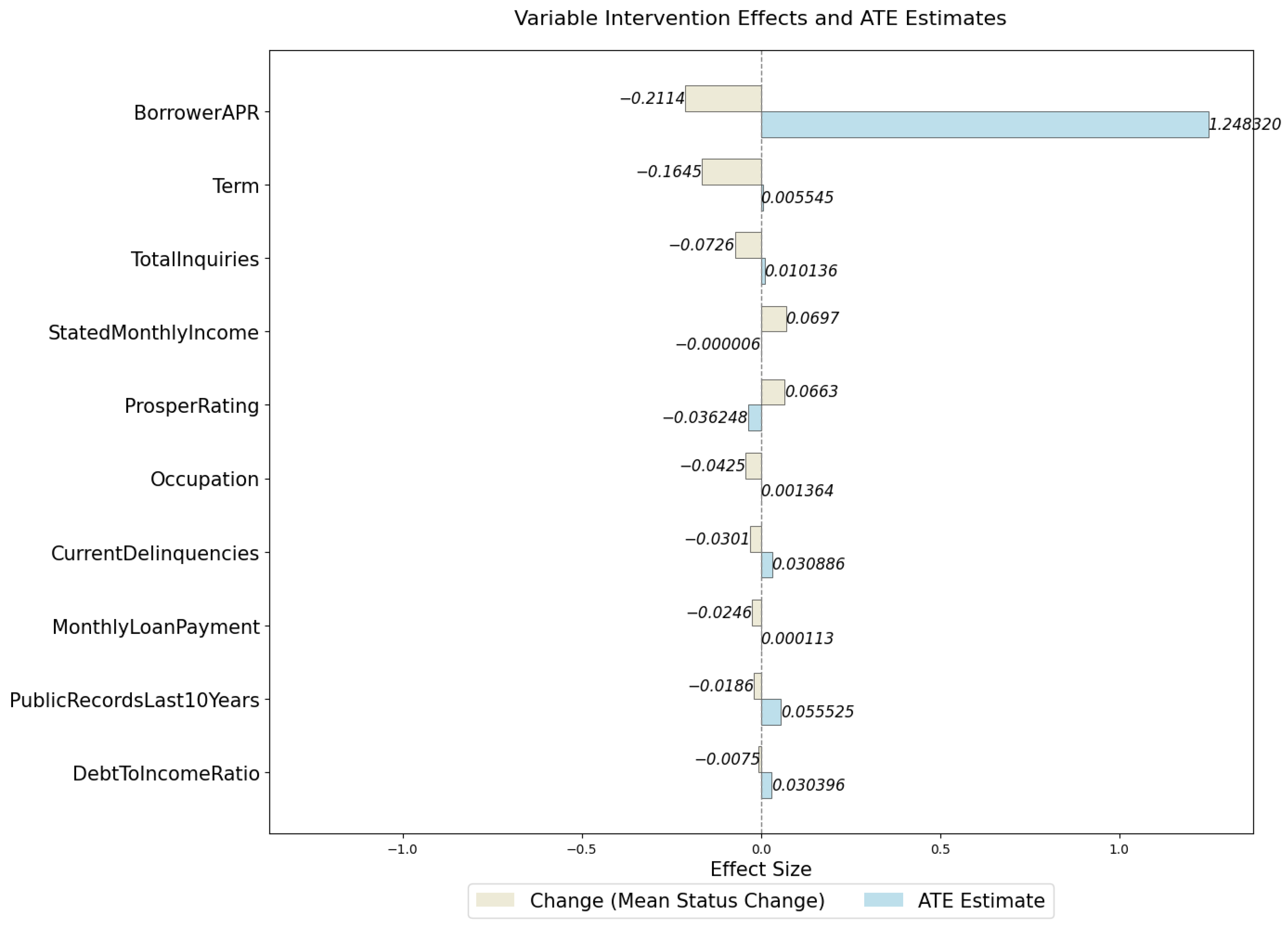
To visualize the direction of causal effects, we use stacked bar charts. The main text reports results for dataset D1 (Figure 3), while complete visualizations for datasets D2–D4 are provided in Appendix A (Figure A4, Figure A5 and Figure A6). For D1, early_return_amount exhibits the most significant negative causal effect, indicating that partial early repayment substantially reduces default risk. Results in Appendix A show consistent and interpretable patterns across the remaining datasets. In D2, Number_Of_Times_90_Days_Late has a strong positive causal effect, suggesting that a history of severe delinquency is a primary driver of default. In D3, both int_rate and term positively affect default probability, implying that higher interest rates and longer maturities increase risk exposure. In D4, Prosper_Rating and Monthly_Loan_Payment demonstrate pronounced positive causal effects, reflecting the critical roles of credit rating and repayment burden in shaping default outcomes. Overall, the estimated causal directions are economically meaningful and structurally consistent across the four datasets, particularly with respect to core risk factors.
Figure 3.
Causal Effect Graph of Influencing Factors in Dataset D1.
It is important to distinguish among three levels of interpretation. Performance improvements and statistical significance support predictive associations at the statistical level only. Causal effect estimation, under the stated identification assumptions, provides directional interpretation of variable impacts. Business implications are derived from a synthesis of these two layers of evidence. Each operates at a different level of explanation and has a distinct scope of applicability.
4.7.3. Counterfactual Explanations and Analysis of Key Feature Impacts
After completing the overall causal effect analysis, it is necessary to further verify the consistency and rationality of the average treatment effect (ATE) estimates and to refine the specific impact directions and magnitudes of different feature changes on the prediction results. This allows us to demonstrate “how the default probability would change if a key feature value of a customer (such as reducing their Number_Of_Times_90_Days_Late) were altered” and “which variable to intervene in would be most effective”, thereby providing a direct basis for personalized risk intervention. On the basis of stable causal features and interaction terms, this section designs a counterfactual explanation analysis framework. By generating counterfactual instances for default risk prediction results, not only can the impact of feature perturbations on changes in default probability be intuitively displayed, but key factors affecting the default outcome and potential intervention directions can also be identified in combination with causal pathways. This series of analyses completes causal effect estimation via the CausalForestDML method, providing more detailed, transparent, and actionable interpretive support for credit risk modeling.
To increase the credibility of causal effect estimates, this section employs the DoWhy framework to estimate ATE for each treatment variable while introducing counterfactual simulations to validate the estimation results. In each experimental round, the ATE is first calculated through the causal model to measure the expected average change in the outcome variable Y when the treatment variable T increases by one unit. A logistic regression prediction model is subsequently constructed to simulate the intervention scenario where the treatment variable is artificially set to 0 while keeping other variables constant to obtain the average change in the default rate before and after the intervention. The specific experimental results are shown in Table 13.
Table 13.
Counterfactual explanation analysis results.
Based on the estimates reported in Table 12, we construct counterfactual explanation plots to visualize intervention effects. For brevity, the main text presents only the intervention results for the D1 dataset (Figure 4), while the corresponding results for D2–D4 are provided in Appendix A Figure A7, Figure A8 and Figure A9. As shown in the figures, although the magnitude of the average treatment effect (ATE) estimated by DoWhy differs from the change in default probability simulated via logistic regression, both methods yield consistent directional effects for the causally identified variables. In other words, the sign of the risk shift under intervention remains stable across estimation frameworks. This consistency suggests that the inferred intervention variables exert robust and directionally coherent effects on default outcomes.
Figure 4.
Counterfactual Explanation for Dataset D1.
Notably, since counterfactual simulations rely on linear prediction models such as logistic regression, they essentially provide an approximate estimation of the intervention outcomes under the assumption of a linear model. Therefore, when there are nonlinear intervention paths or complex interactions between the treatment variable and the outcome variable, the simulation process may not fully capture the nonlinear response of the true causal effect, leading to significant numerical differences from the ATE estimated by the double machine learning method in the DoWhy framework.
Nevertheless, the results of counterfactual simulations still hold important reference value. On the one hand, the simulation process is visually clear and can provide an intuitive explanation of “how the impact on the outcome variable would change if the variable were artificially set to 0”; on the other hand, given the consistency in the intervention direction, even if there are numerical deviations, counterfactual simulations can still verify the robustness of the causal direction and assist in judging whether the treatment variable has a stable effect on the outcome variable. Therefore, using counterfactual simulations as a supplementary validation for the DML estimation results helps enhance the interpretability and application value of causal conclusions.
4.7.4. Counterfactual Intervention on a Specific Variable
To further demonstrate the model’s intervention-level interpretability, we construct an individual-level counterfactual analysis using the interest rate variable (Interest) from the CCF dataset as an example. Specifically, we simulate a proportional reduction in the interest rate while holding all other covariates constant, and compare the predicted default probabilities before and after the intervention.
We first train a global surrogate prediction model based on the causally selected features used in the primary model. This surrogate approximates the response surface between feature variations and default risk. From the empirical data, we then select representative defaulted individuals whose interest rates exceed the sample median. For each selected individual, we generate a counterfactual instance by reducing the interest rate by 50%, and compute the corresponding change in predicted default probability. The simulation results are presented in Figure 5.
Figure 5.
Individual Counterfactual Simulation Results.
The results indicate that, conditional on other risk factors remaining fixed, a reduction in the interest rate leads to a substantial decrease in predicted default probability at the individual level. The magnitude of risk reduction exhibits heterogeneity across individuals. The direction of these changes is consistent with the estimated causal effects reported earlier, providing intervention-based validation of the structural influence of interest rates on default risk.
We emphasize that this counterfactual analysis serves to illustrate the model’s intervention interpretability. Its conclusions rely on the underlying identification assumptions and the surrogate model approximation, and should be interpreted as a quantitative demonstration of structural risk trends rather than as prescriptive policy guidance.
4.8. Ablation Study
4.8.1. Experimental Setup
To further verify the actual contributions of each feature processing step to model performance, this paper designs a systematic ablation study based on the optimal and most stable logistic regression + causal feature enhancement scheme. By progressively removing or adding feature selection modules, the incremental effects of each step on the final prediction outcomes are quantitatively assessed. The specific design is as follows:
Experiment 1: Models are built and evaluated directly via all the features after initial preprocessing, without IV value screening, XGBoost screening, stable causal feature selection, or interaction feature construction.
Experiment 2: The initial feature screening step based on IV values is removed, and all original features are used for subsequent processes.
Experiment 3: IV screening is retained, but the XGBoost feature importance screening is skipped, proceeding directly to causal feature selection.
Experiment 4: After XGBoost screening, the PC algorithm screening and causal interaction feature construction are skipped, and models are built using the remaining features.
Experiment 5: Models are built after IV screening, XGBoost feature importance screening, PC algorithm screening, and causal interaction feature construction.
The performance of each control group is compared with that of the complete modeling process to quantify the marginal improvement effects of each module on the final predictive capability.
In the ablation study, the following three types of metrics are comprehensively used to systematically evaluate model performance:
F1 score: A measure that considers both precision and recall in the context of class imbalance.
AUC: An assessment of the model’s ability to distinguish between classes at different decision thresholds.
G-mean: An evaluation of the model’s balanced performance on both positive and negative classes.
4.8.2. Analysis of Ablation Study Results
The results of the ablation study are shown in Table 14.
Table 14.
Comparison of Ablation Study Results.
On the basis of Table 12, the numerical comparisons of F1 scores, AUC values, and G-means across different experiments are illustrated in Figure 6. It can be intuitively observed from the figure that different feature processing modules contribute to model performance improvements to varying degrees. A systematic analysis of the ablation study results across the four datasets is provided below:
Figure 6.
Line charts of changes in the core metrics across different experiments on the four datasets.
- (1)
- Causal feature selection and interaction feature construction are key to model performance enhancement
In Experiment 4, where the PC algorithm’s causal feature selection and interaction feature construction were removed, the model performance generally declined significantly. Particularly in Dataset D2, the F1 score decreased by 0.062, and it was also notably lower than that in Experiment 5 (the complete modeling process) for the other datasets. This result indicates that stable feature selection and interaction feature construction under causal pathways significantly enhance the model’s ability to capture complex causal relationships, effectively improving the model’s discriminative and generalization capabilities. This is the most critical part of the entire feature engineering process.
- (2)
- IV Initial screening has a limited impact on model performance improvement
Compared with Experiment 1, the core metrics for distinguishing between default and nondefault samples in Experiment 2 showed minimal changes across all datasets. This suggests that the noise reduction effect of IV value screening is limited in the current data environment. Potential explanations include the following: First, the proportion of irrelevant or noisy variables in the original feature set may be inherently low. Second, subsequent XGBoost feature importance screening and PC algorithm selection demonstrate robust redundancy elimination capabilities, thereby reducing the marginal contribution of preliminary IV screening.
- (3)
- XGBoost feature importance screening provides an optimal initial feature set for causal screening
When Experiment 3 is compared with Experiment 5, in Datasets D1 and D3, the model F1 scores decrease by 0.0101 and 0.0123, respectively. Although the changes were small but consistent, this finding indicates that the role of XGBoost screening in improving feature quality is limited. However, its value lies mainly in providing a more compact and strongly correlated input feature set for PC causal structure learning, thereby indirectly enhancing the effectiveness of causal inference.
- (4)
- Dataset D3 has the smallest performance variations across different experimental groups.
In Experiments 1 to 5, the F1 scores, AUC values, and G-means values of Dataset D3 show almost no significant fluctuations. This suggests that the original features of this dataset already have a high information density, and further feature engineering cannot significantly improve the model’s performance.
In summary, the ablation study fully validates the central role of causal feature selection and interaction feature construction in complex data modeling. It also reveals that the marginal effects of traditional screening methods vary with different data characteristics. This finding provides important evidence for optimizing feature engineering strategies.
5. Conclusions
This paper presents a unified framework for credit default prediction that integrates causal feature selection, interaction-aware feature construction, and interpretability. The framework improves predictive performance, stability, and transparency, and is validated on multiple real-world credit datasets. The main findings are summarized as follows.
- (1)
- Causal feature identification via perturbation-enhanced PC.
Unlike conventional screening methods based on information value or correlation, we employ a perturbation-enhanced PC algorithm to uncover causal relationships among variables. By combining multi-scale sample perturbations with bootstrap resampling, we identify stable causal parents of the target variable and effectively eliminate spurious correlations.
- (2)
- Interaction construction over stable causal features.
High-order interaction terms are constructed on top of the stable causal feature set to improve the model’s ability to capture nonlinear mechanisms. Only interactions along validated causal paths are retained, reducing redundancy and mitigating multicollinearity. Experiments across multiple datasets show that this strategy consistently identifies causally relevant variables strongly associated with default behavior.
- (3)
- Model generality and robustness evaluation.
We evaluate the proposed features using Logistic Regression, CART, Random Forest, XGBoost, and LightGBM, with hyperparameters tuned via grid search and cross-validation. To address class imbalance, performance is assessed using F1-score, AUC, and G-mean. Results indicate that the causal enhancement strategy improves performance in most models, with the largest gains observed in Logistic Regression, suggesting that causal feature extraction significantly strengthens the expressive power of traditional linear models.
- (4)
- Causal effect estimation and counterfactual explanation.
We construct a causal identification and effect estimation pipeline by combining causal path analysis with CausalForestDML. This enables quantification of both direct and indirect effects of key variables on default probability. A counterfactual explanation mechanism is further introduced to simulate how changes in critical variables alter predicted outcomes, providing actionable decision support.
- (5)
- Statistical validation and ablation analysis.
Paired-sample t-tests and Cohen’s d effect sizes are used to evaluate the statistical significance of the causal enhancement strategy. Ablation studies quantify the contribution of each module. Logistic Regression with causal enhancement significantly outperforms baselines across four datasets, with causal feature selection and interaction construction identified as the primary drivers of improvement.
Despite these results, several limitations remain:
- (1)
- Dependence on the PC algorithm.
Causal discovery relies on the PC algorithm, which is sensitive to sample size, distributional properties, and conditional independence assumptions. Future work may integrate multiple causal discovery methods to improve structural robustness [24].
- (2)
- Limited automation in interaction construction.
Interaction features are generated through rule-based procedures, without automated search or advanced nonlinear modeling. Incorporating deep learning or structure search mechanisms [25] could further enhance high-order feature representation.
- (3)
- Operationalization of explanations.
While interpretability is improved, explanatory outputs are not yet fully translated into actionable policy recommendations. Future work can leverage counterfactual reasoning to establish a closed-loop framework linking features, interventions, and changes in default probability, thereby providing stronger support for credit decision-making.
Author Contributions
Conceptualization, T.C. and J.H.; methodology, R.Z.; software, R.Z.; validation, J.H.; formal analysis, R.Z.; data curation, T.C.; writing—original draft preparation, T.C. and R.Z.; writing—review and editing, J.H.; visualization, R.Z. All authors have read and agreed to the published version of the manuscript.
Funding
This research was funded by Major Program of National Philosophy and Social Science Foundation of China (grant number: 22&ZD162).
Data Availability Statement
The data used to support the findings of this study are available from the corresponding author upon request.
Conflicts of Interest
The authors declare no conflicts of interest.
Appendix A
Table A1.
Results of the direct and indirect paths affecting the defaults in D2–D4 dataset.
Figure A1.
Causal Pathway Diagram for Dataset D2.
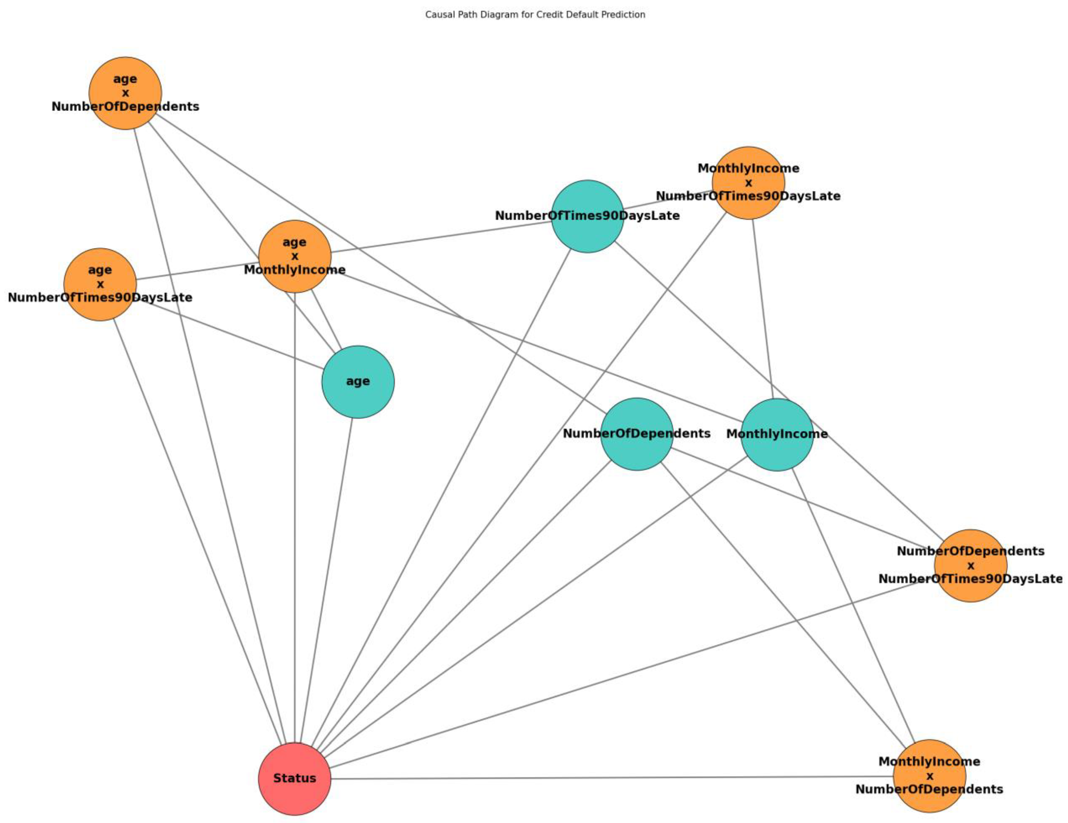
Figure A2.
Causal Pathway Diagram for Dataset D3.
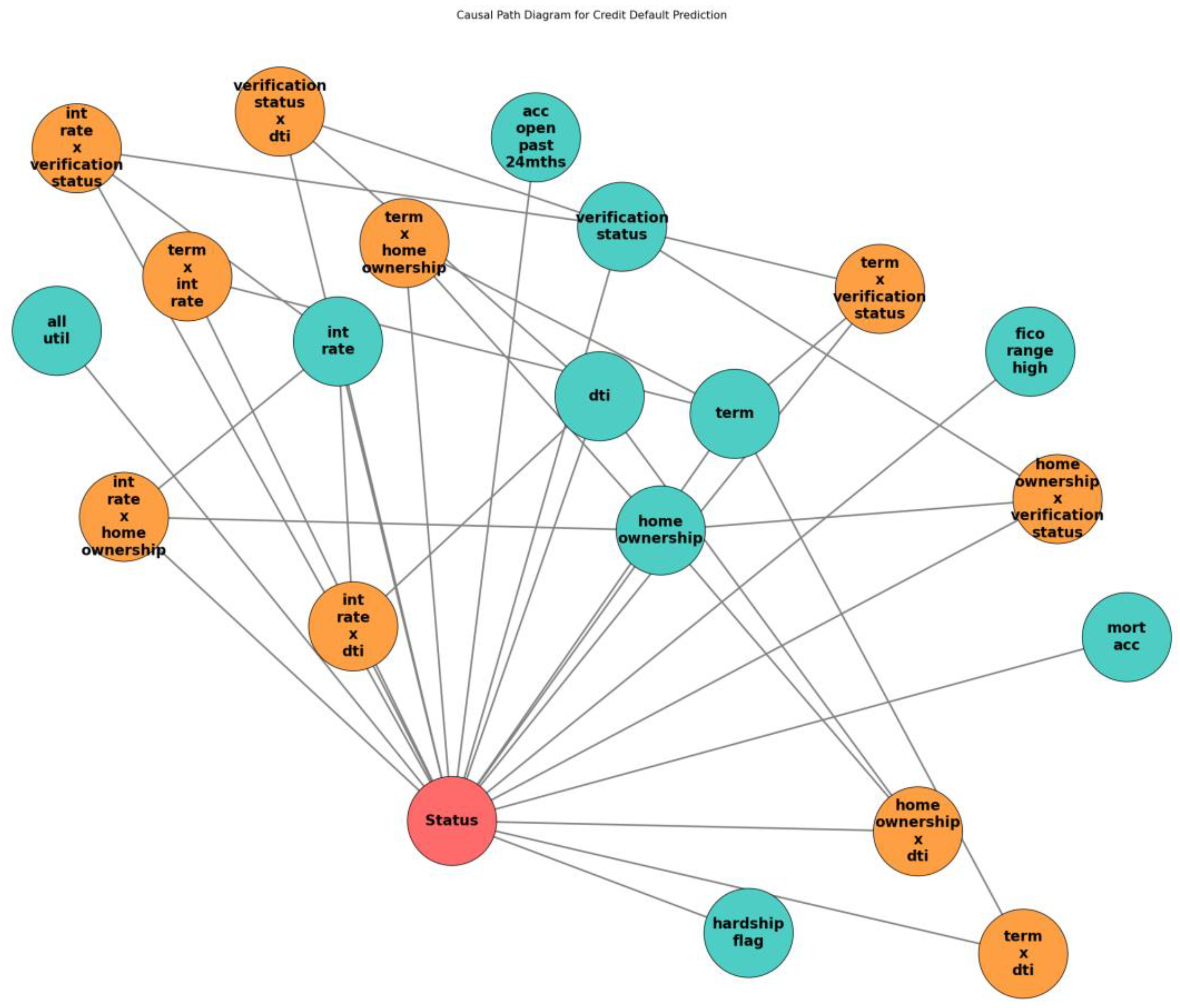
Figure A3.
Causal Pathway Diagram for Dataset D4.
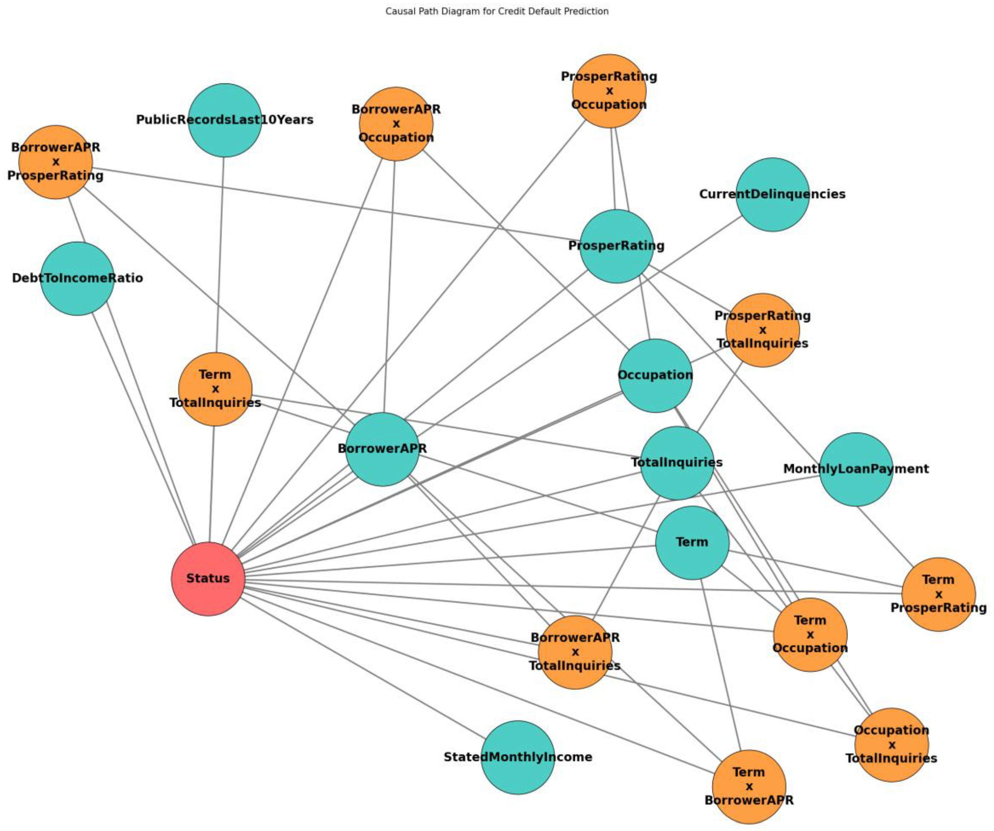
Figure A4.
Causal Effect Graph of Influencing Factors in Dataset D2.
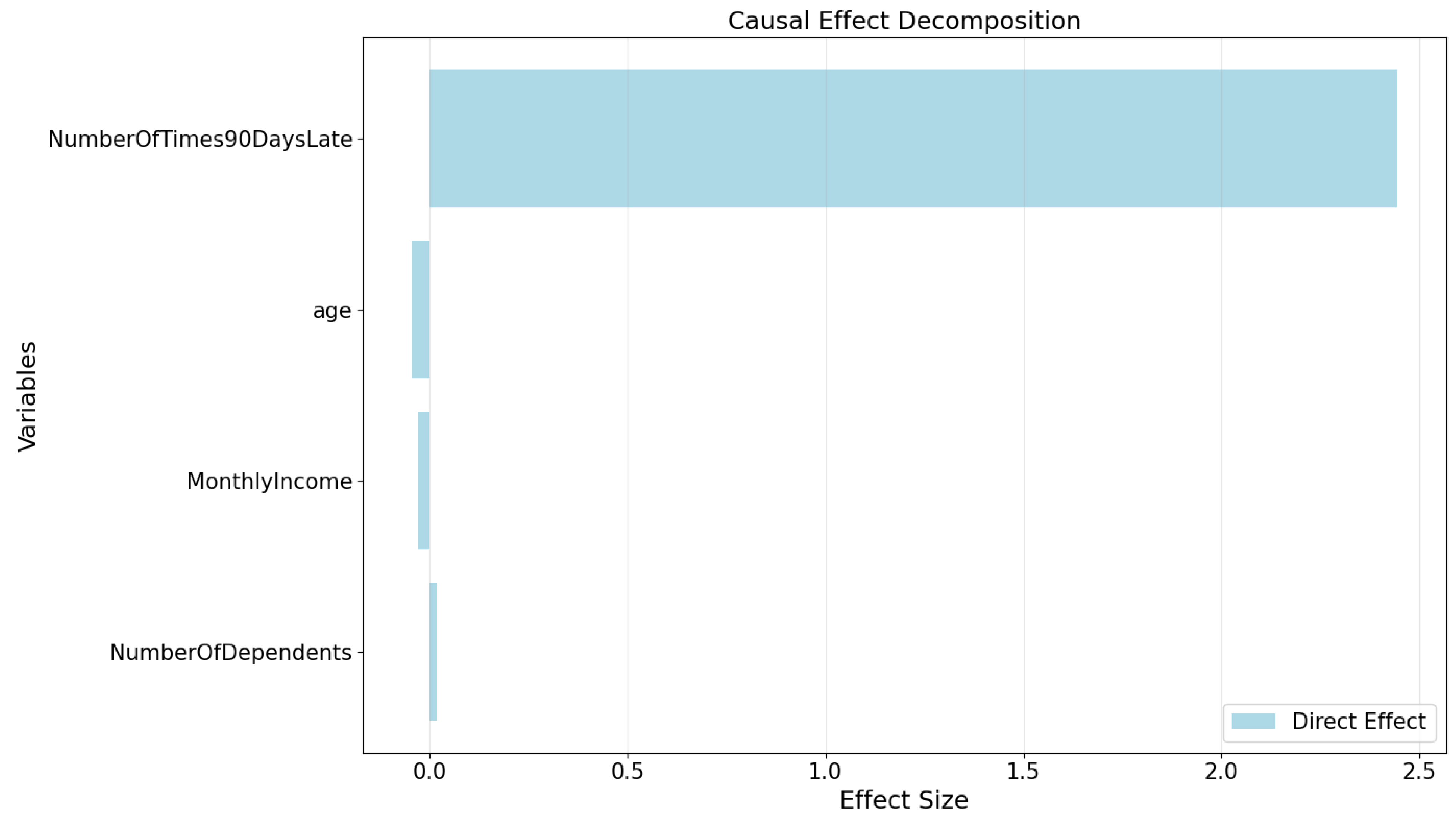
Figure A5.
Causal Effect Graph of Influencing Factors in Dataset D3.
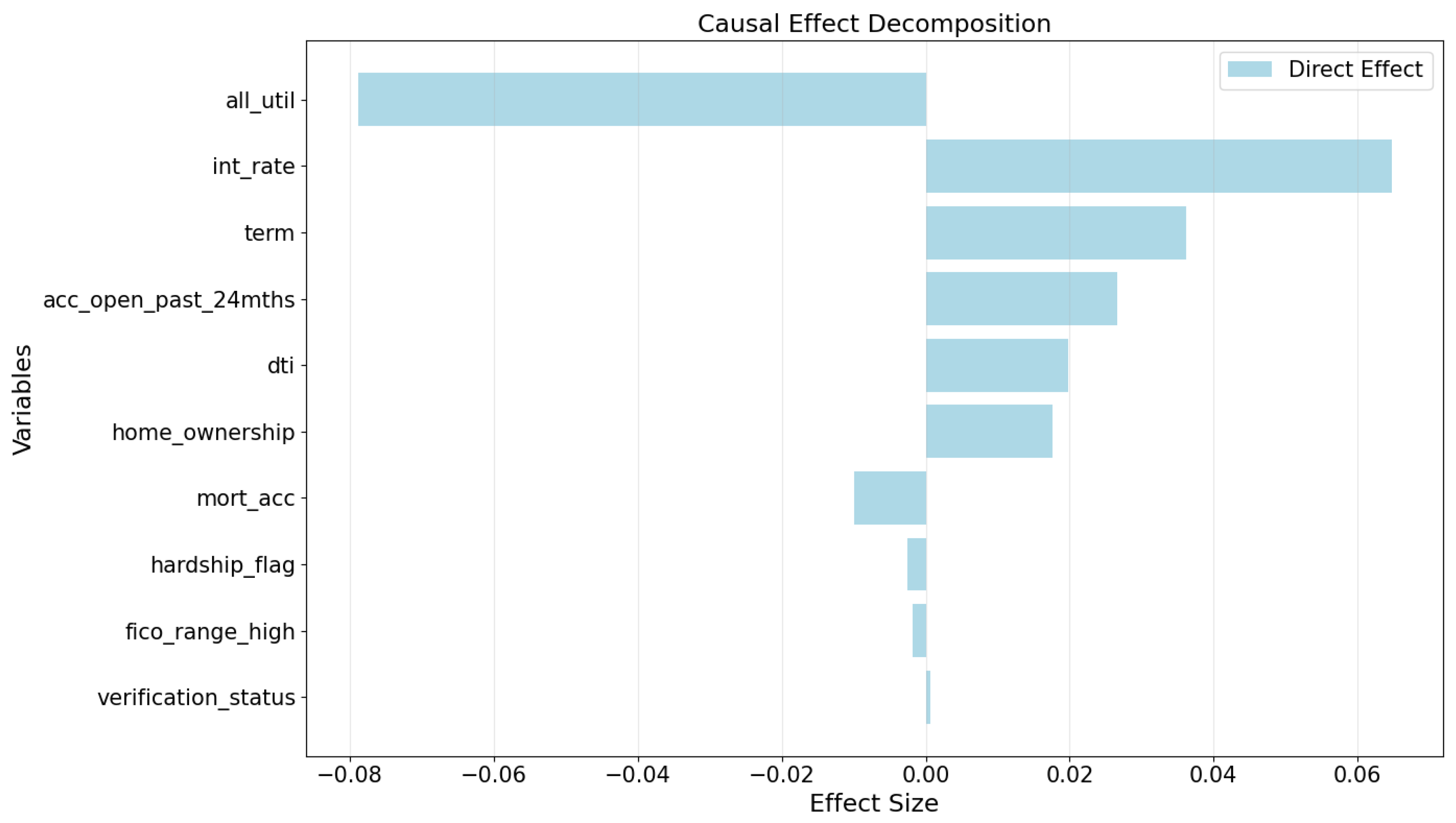
Figure A6.
Causal Effect Graph of Influencing Factors in Dataset D4.
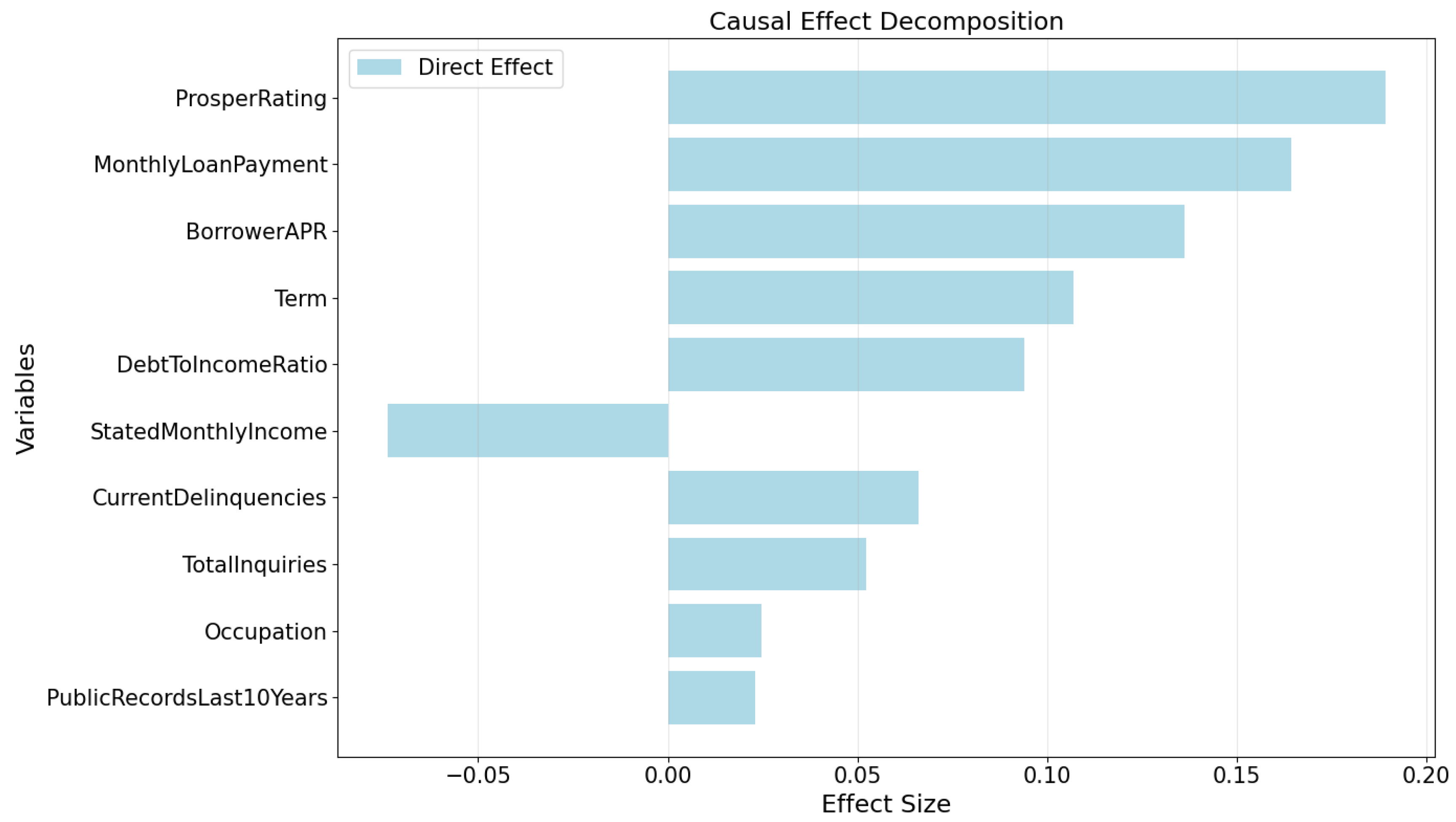
Figure A7.
Counterfactual Explanation for Dataset D2.
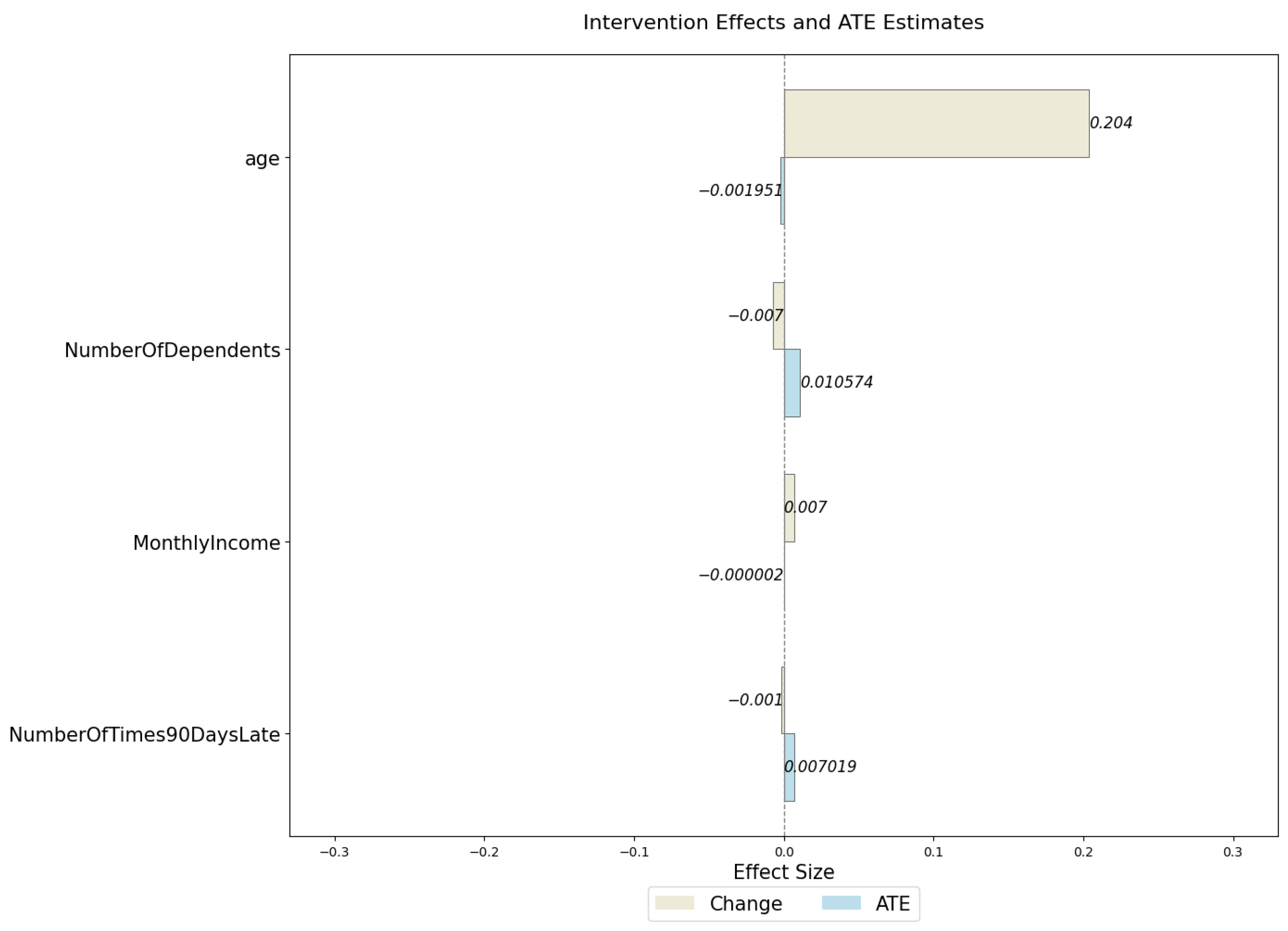
Figure A8.
Counterfactual Explanation for Dataset D3.
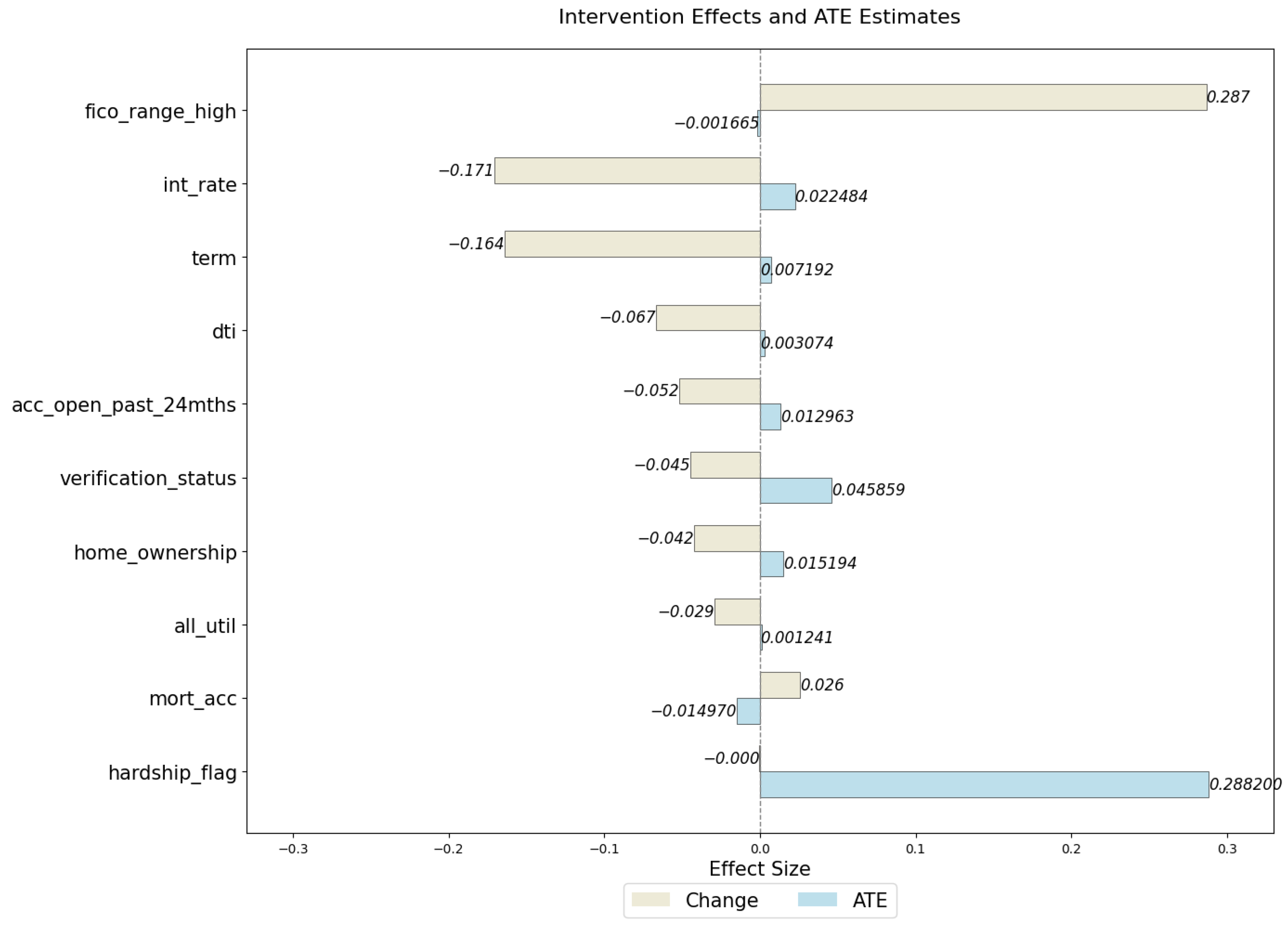
Figure A9.
Counterfactual Explanation for Dataset D4.
References
- Sohn, S.Y.; Kim, D.H.; Yoon, J.H. Technology credit scoring model with fuzzy logistic regression. Appl. Soft Comput. 2016, 43, 150–158. [Google Scholar] [CrossRef] [Scilit]
- Chang, Y.; Chang, K.; Lin, Y. Establishment of business loan default prediction model by integrating survival analysis with logistic regression. Sci. Iran. 2024, 31, 2139–2147. [Google Scholar] [CrossRef] [Scilit]
- Zhou, Y.; Su, X. Credit Risk Prediction of Enterprises Based on Optimal Index Combination. J. Syst. Manag. 2021, 30, 817–838. (In Chinese) [Google Scholar]
- Zhang, X.; Zhang, T.; Hou, L.; Liu, X.; Guo, Z.; Tian, Y.; Liu, Y. Data-Driven Loan Default Prediction: A Machine Learning Approach for Enhancing Business Process Management. Systems 2025, 13, 581. [Google Scholar] [CrossRef] [Scilit]
- Dichev, A.; Zarkova, S.; Angelov, P. Machine Learning as a Tool for Assessment and Management of Fraud Risk in Banking Transactions. J. Risk Financ. Manag. 2025, 18, 130. [Google Scholar] [CrossRef] [Scilit]
- Gao, B.; Balyan, V. Construction of a financial default risk prediction model based on the LightGBM algorithm. J. Intell. Syst. 2022, 31, 767–779. [Google Scholar] [CrossRef] [Scilit]
- Zhang, Y.; Zhuo, P.; Liu, Z.; Liu, W.; Song, Y. Credit Default Prediction Model Based on Transformer Encoder and Residual Network. Comput. Appl. 2024, 44, 324–329. (In Chinese) [Google Scholar] [CrossRef] [Scilit]
- Yan, Z.P.; Qu, H.W.; Chen, C.; Lv, X.Y.; Zuo, E.G.; Wang, K.; Cai, X.L. WIGNN: An adaptive graph-structured reasoning model for credit default prediction. Eng. Appl. Artif. Intell. 2025, 139, 109597. [Google Scholar] [CrossRef] [Scilit]
- Chi, G.; Wang, S.; Wang, Y. Research on Early Warning of Default Risk of Listed Companies Based on Stacking Method. Syst. Eng.-Theory Pract. 2025, 45, 481–502. (In Chinese) [Google Scholar]
- Chugh, B.; Malik, N.; Gupta, D.; Alkahtani, B.S. A probabilistic approach driven credit card anomaly detection with CBLOF and isolation forest models. Alex. Eng. J. 2025, 114, 231–242. [Google Scholar] [CrossRef] [Scilit]
- Ma, C.; Sun, H.Y.; Wang, S.F.; Lu, S.L.; Li, J.Y. Bond Default Prediction Based on Deep Learning and Knowledge Graph Technology. IEEE Access 2021, 9, 12750–12761. [Google Scholar] [CrossRef] [Scilit]
- Kong, M.; Li, R.; Wang, J.; Li, X.; Jin, S.Z.; Xie, W.Y.; Hou, M.Z.; Cao, C. CFTNet: A robust credit card fraud detection model enhanced by counterfactual data augmentation. Neural Comput. Appl. 2024, 36, 8607–8623. [Google Scholar] [CrossRef] [Scilit]
- Zandi, S.; Korangi, K.; Óskarsdottir, M.; Mues, C.; Bravo, C. Attention-based dynamic multilayer graph neural networks for loan default prediction. Eur. J. Oper. Res. 2025, 321, 586–599. [Google Scholar] [CrossRef] [Scilit]
- Sun, W.X.; Zhang, X.T.; Li, M.H.; Wang, Y. Interpretable high-stakes decision support system for credit default forecasting. Technol. Forecast. Soc. Change 2023, 196, 122825. [Google Scholar] [CrossRef] [Scilit]
- Kagaba, D.; Busingye, C.; Nansamba, B.; Jingo, D.; Marvin, G. Explainable deep ensemble learning for improved credit default prediction. In Proceedings of the 2024 Sixteenth International Conference on Contemporary Computing; Association for Computing Machinery: New York, NY, USA, 2024; pp. 256–270. [Google Scholar]
- Arias-Serna, M.A.; Quiza-Montealegre, J.J.; Móntes-Gómez, L.F.; Uribe Clavijo, L.; Orozco-Duque, A.F. Explainable Machine Learning Models for Credit Rating in Colombian Solidarity Sector Entities. J. Risk Financ. Manag. 2025, 18, 489. [Google Scholar] [CrossRef] [Scilit]
- Pearle, J. Causality: Models, Reasoning, and Inference, 2nd ed.; Cambridge University Press: Cambridge, UK, 2009. [Google Scholar]
- Bakir, M.R.; Cetin, M.A.; Bakirtas, I. Revisiting the macroeconomic determinants of non-performing loans with a deep learning technique with causal inference: Evidence from Türkiye. Borsa Istanb. Rev. 2025, 25, 541–551. [Google Scholar] [CrossRef] [Scilit]
- Peng, M.; Stern, E.R.; Hu, H. Forecasting China bond default with severe class-imbalanced data: A simple learning model with causal inference. Econ. Model. 2025, 144, 106985. [Google Scholar] [CrossRef] [Scilit]
- Li, Y.; Yan, K.Y. Prediction of bank credit customers churn based on machine learning and interpretability analysis. Data Sci. Financ. Econ. 2025, 5, 19–34. [Google Scholar] [CrossRef] [Scilit]
- Noh, M.J.; Kim, Y.S. Diabetes prediction through linkage of causal discovery and inference model with machine learning models. Biomedicines 2025, 13, 124. [Google Scholar] [CrossRef] [Scilit] [PubMed]
- Song, C.Y.; Shi, Y.T.; Li, M.; Wu, L.; Xiong, X.R.; Liu, J.Y.; Xia, D.S. An efficient catalyst screening strategy combining machine learning and causal inference. J. Environ. Manag. 2025, 377, 124665. [Google Scholar] [CrossRef] [Scilit] [PubMed]
- Founta, K.; Dafou, D.; Kanata, E.; Mues, T.; Zanos, T.; Gounaris, A.; Xanthopoulos, K. Gene targeting in amyotrophic lateral sclerosis using causality-based feature selection and machine learning. Mol. Med. 2023, 29, 12. [Google Scholar] [CrossRef] [Scilit] [PubMed]
- Chen, T.; Gu, H.; Chen, Y.; Ni, L. Credit Risk Identification Algorithm Based on BaggingFCBF-TCN. Concurr. Comput. Pract. Exp. 2026, 38, e70498. [Google Scholar] [CrossRef] [Scilit]
- Chen, T.; Yang, X.; Yang, Z.; Fang, J. A credit card fraud detection model based on a stacked temporospatial graph attention residual network. J. Credit Risk 2026, 22, 1–41. [Google Scholar] [CrossRef] [Scilit]
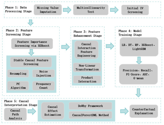
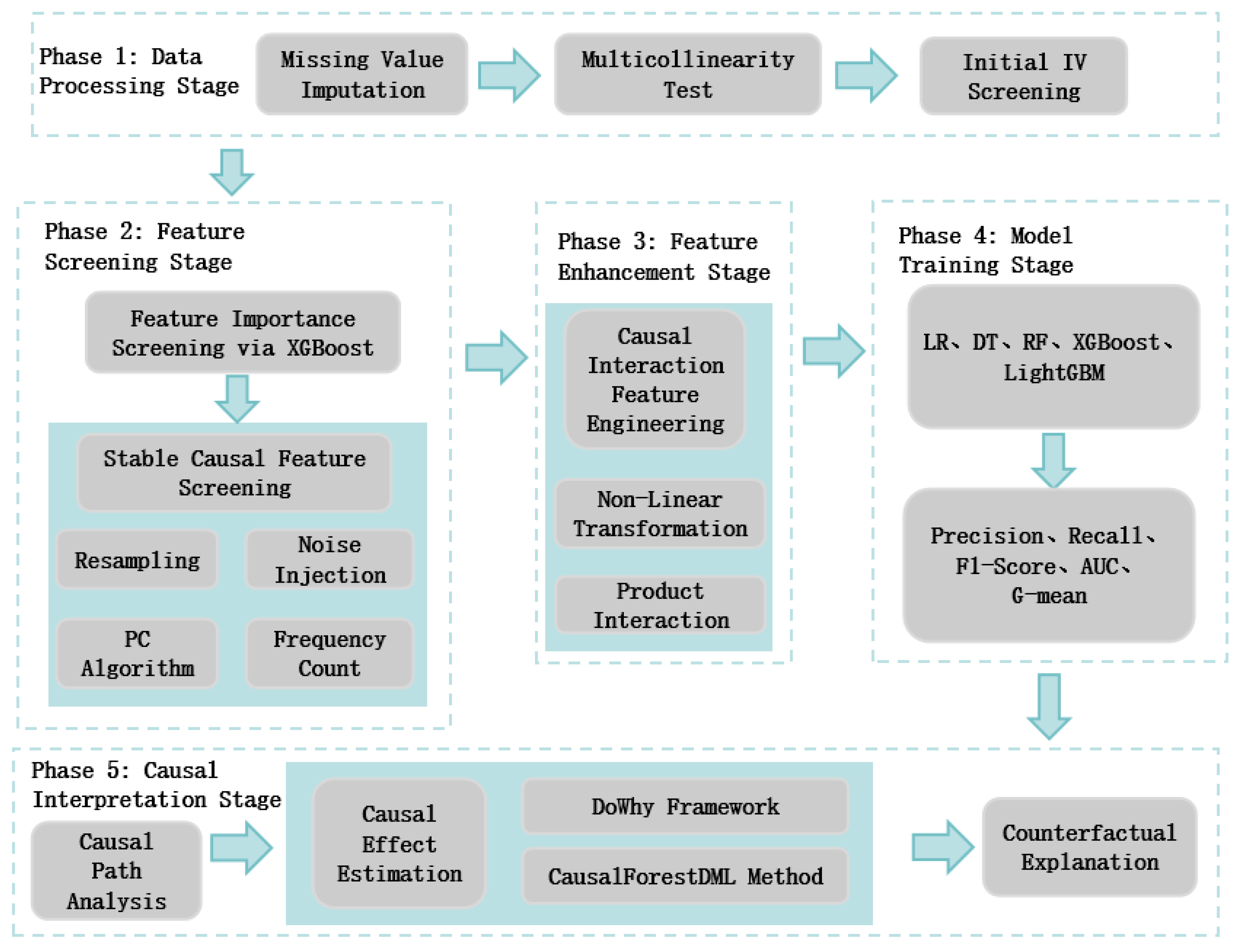
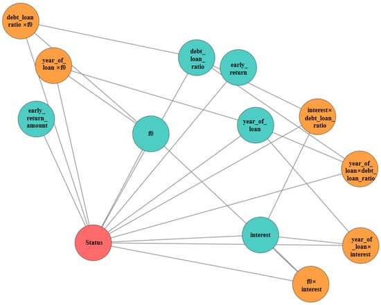
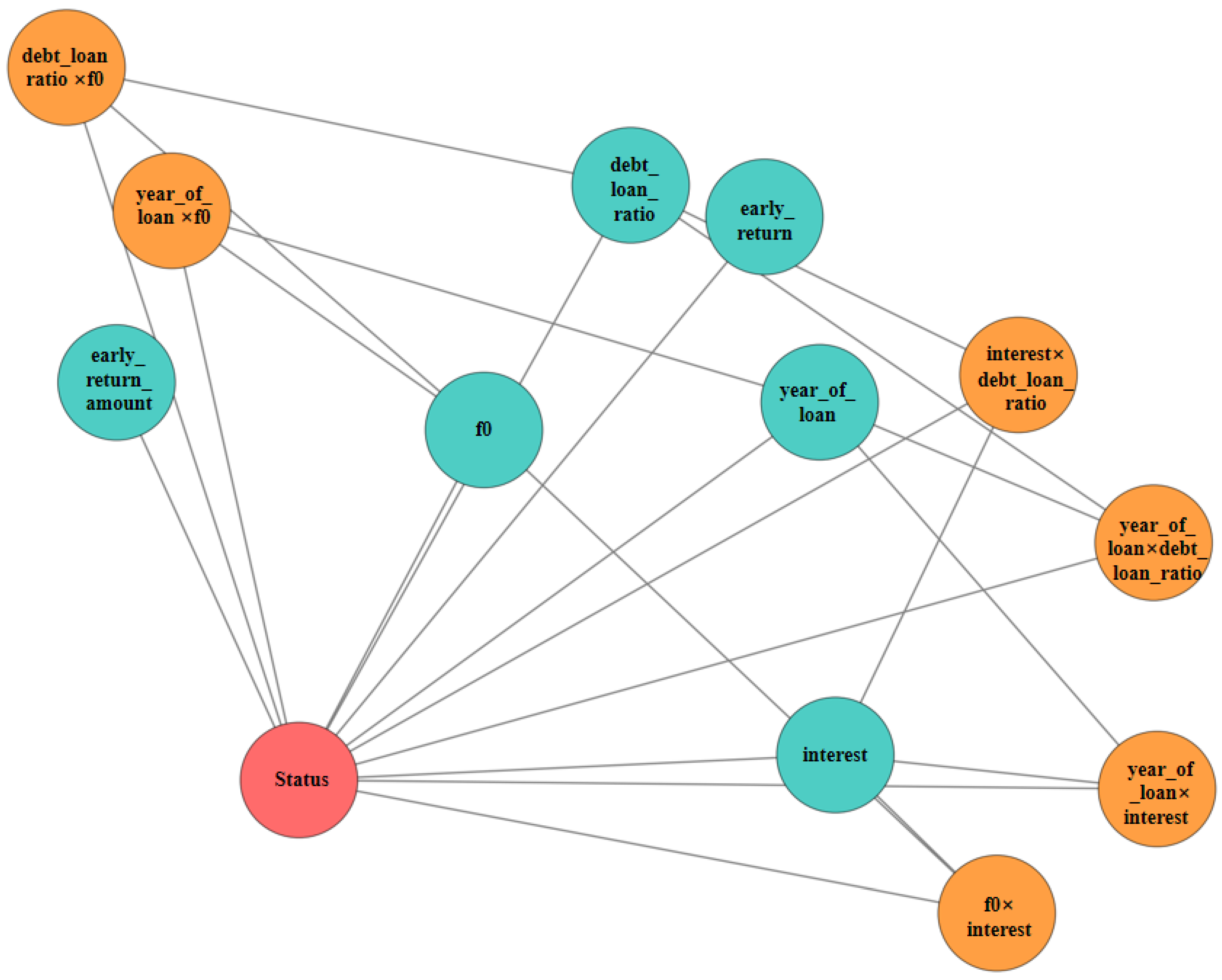
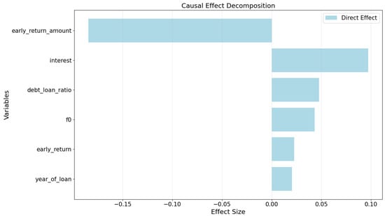
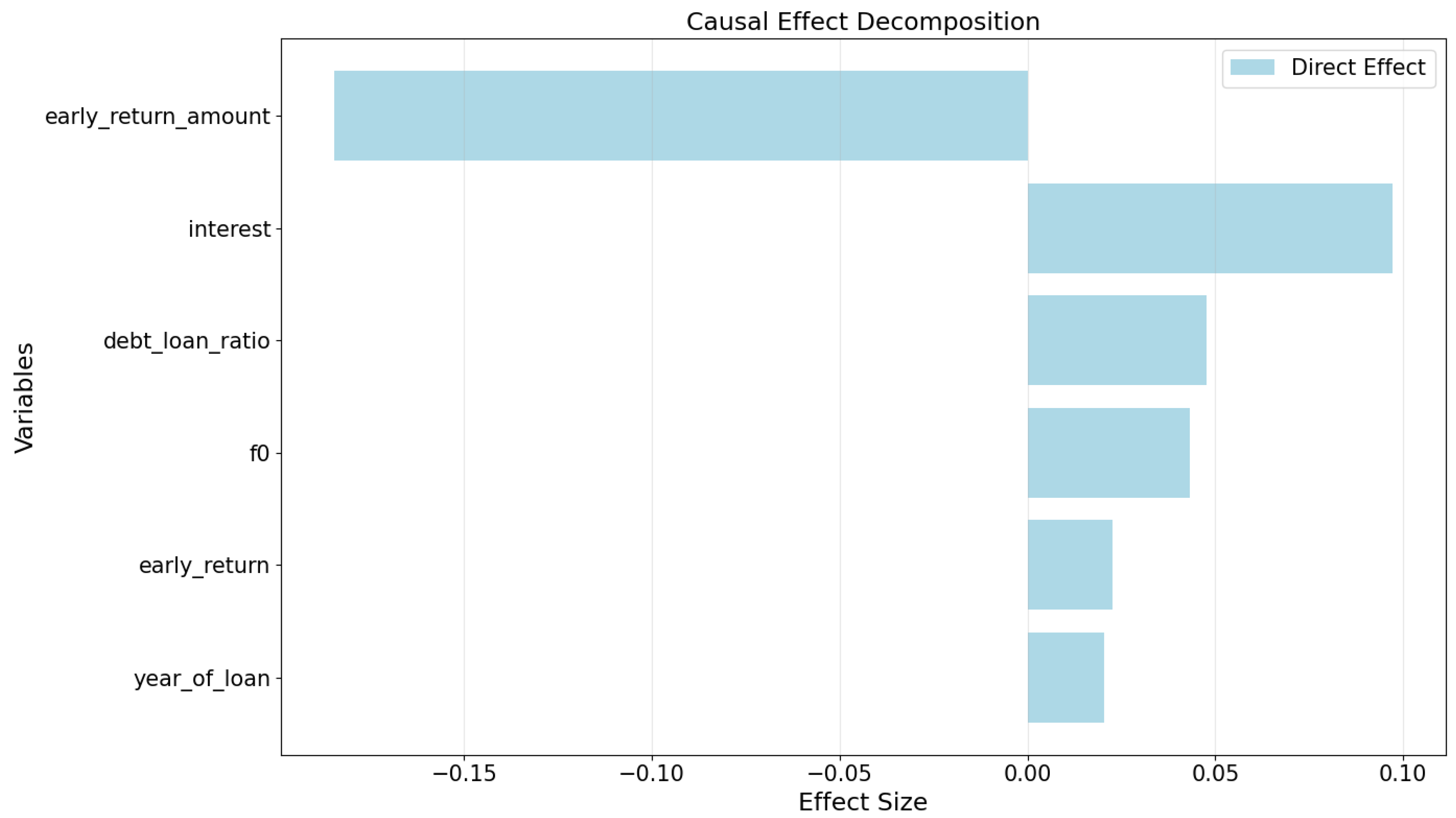
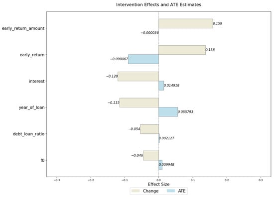
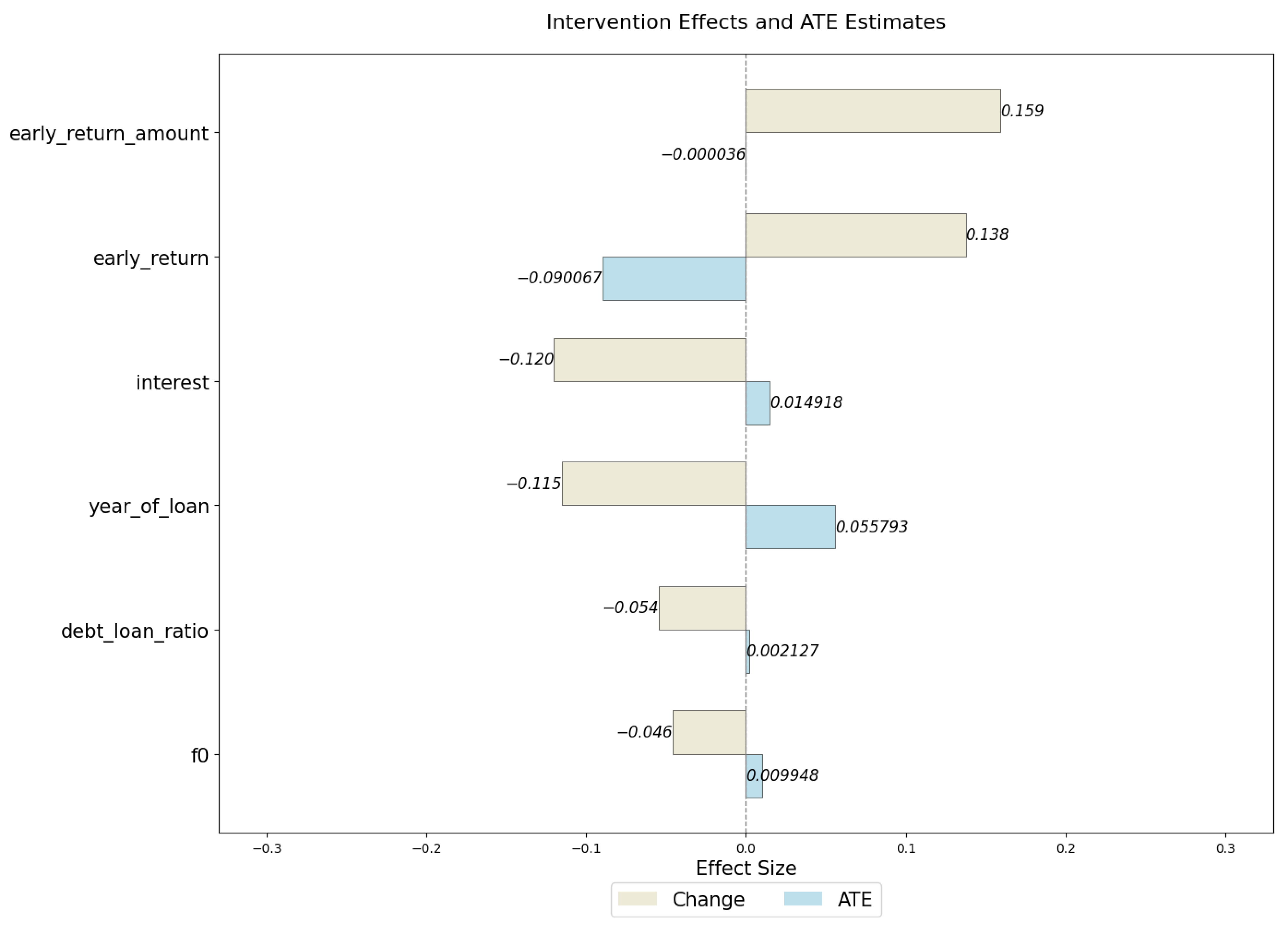
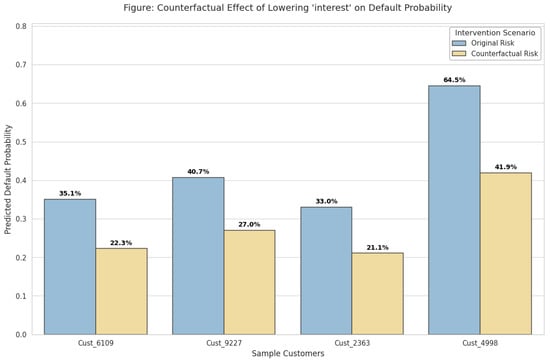
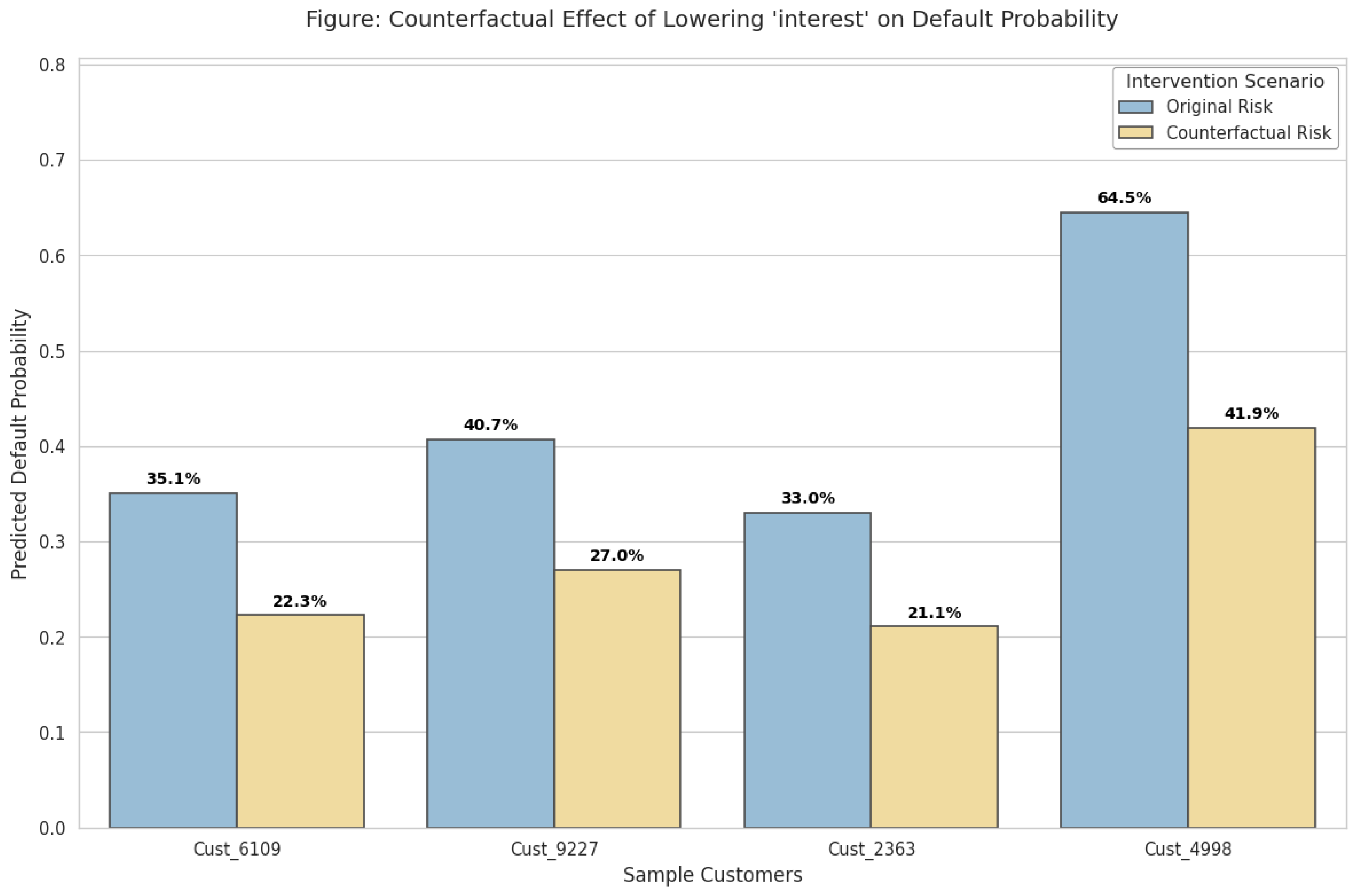
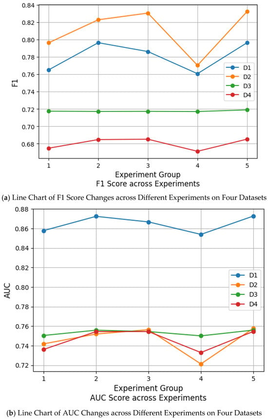
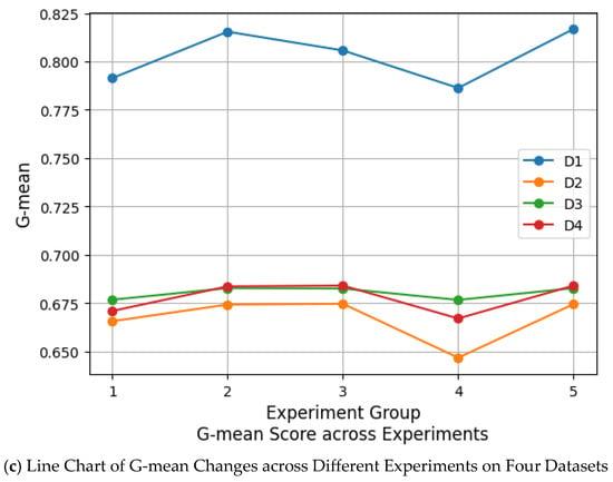
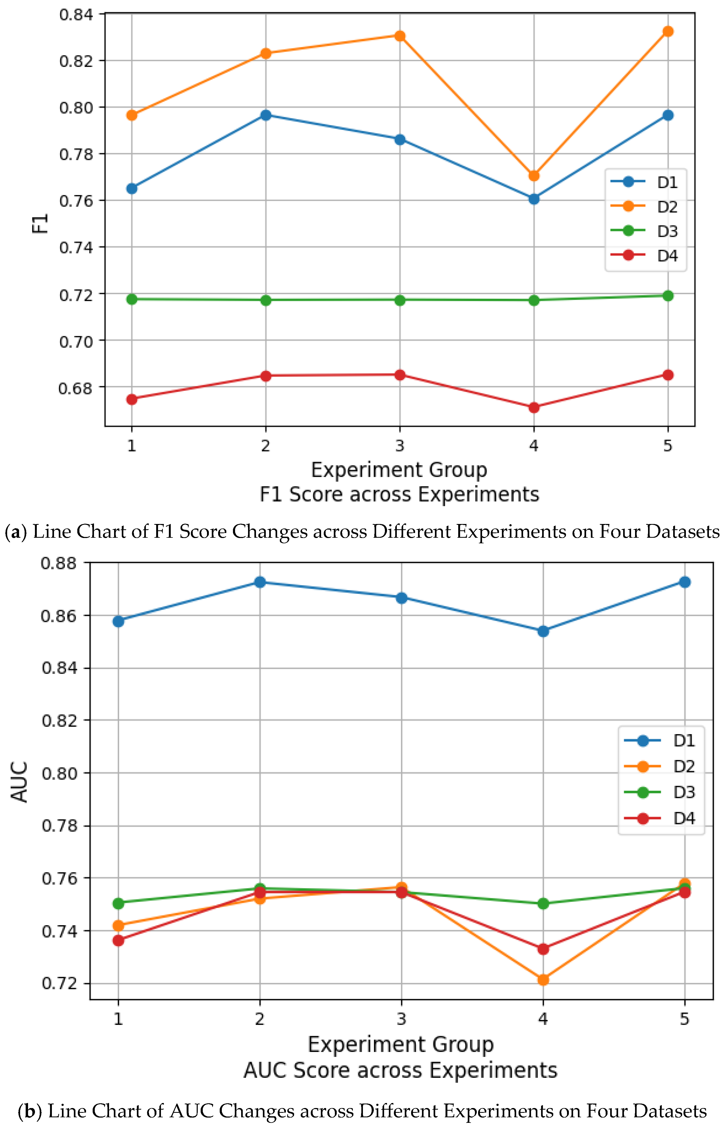
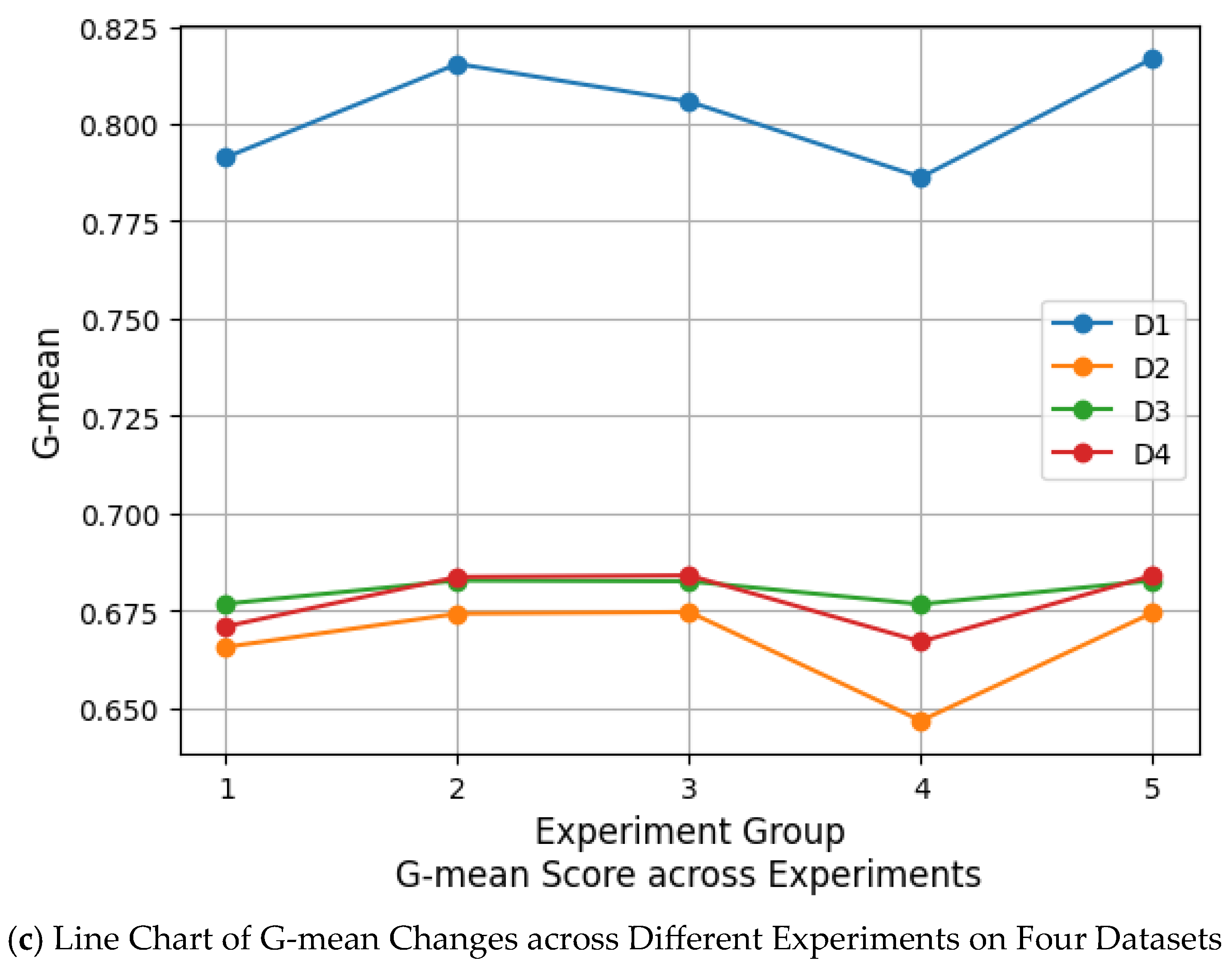

Disclaimer/Publisher’s Note: The statements, opinions and data contained in all publications are solely those of the individual author(s) and contributor(s) and not of MDPI and/or the editor(s). MDPI and/or the editor(s) disclaim responsibility for any injury to people or property resulting from any ideas, methods, instructions or products referred to in the content. |
© 2026 by the authors. Licensee MDPI, Basel, Switzerland. This article is an open access article distributed under the terms and conditions of the Creative Commons Attribution (CC BY) license.