


Highlights
Please indicate how your work links to systems science via your contributions to systems practice, theory, and/or methodology.
- The study frames bridge vibration monitoring as a cyber–physical system involving coupled sensing, cascade communication, gateway storage, temporal reconstruction, and signal-processing layers.
- The proposed evaluation approach emphasizes system-level performance through fixed-grid temporal continuity, valid-window availability, relative timing scope, and bounded vibration-activity indicators.
What are the main findings and/or the implications of the main findings?
- Laboratory and field results show that end-to-end temporal continuity, rather than sensor acquisition alone, is the main operational constraint for the proposed low-cost shared-gateway architecture.
- The selected valid windows showed a within-session contrast between local low-activity and higher-vibration intervals, but the evidence supports temporary vibration-activity monitoring rather than modal identification, diagnosis, warning, or long-term SHM.
Abstract
Municipal bridge management requires accessible monitoring approaches that provide objective information on vibration activity under operational conditions. This study develops and evaluates a low-cost cyber–physical sensing architecture using the Lusitania Bridge in Viña del Mar, Chile, as a case study. The system integrates four ESP32/MPU9250 sensing nodes, cascade Wi-Fi/WebSocket forwarding, a Raspberry Pi 4 gateway with an auxiliary local MPU9250 channel, and structured post-processing. Its contribution is the author-developed system-level integration and bounded field evaluation rather than the novelty of the individual components. In the laboratory shaker test, each remote node occupied 13,560 of 15,001 bins on a fixed 100 Hz grid, corresponding to a 9.61% temporal-continuity deficit; the stored-row rate was 100.023 Hz. Cross-correlation signal lags were within one to two nominal sampling intervals, but these lags are not treated as pure clock-synchronization errors. The field campaign comprised 19 short sessions collected during one experimental day. The mean session-level fixed-grid deficit was 21.04%, with values ranging from 6.83% to 44.09%, showing that end-to-end continuity was the principal operational constraint. Session S18 had the lowest deficit, 6.83%, and 214 valid 30 s windows out of 271 candidates. In S18, a higher-vibration interval showed 0.5–20 Hz band-limited RMS ratios of 1.91–2.86 and band-power increases of 5.6–9.1 dB relative to a low-activity interval. Because the sensors were mounted on the railing and no calibrated reference accelerometer was available, the results support short-duration vibration-activity monitoring and system testing, not global modal identification, damage diagnosis, warning capability, or long-term SHM.
1. Introduction
Bridge infrastructure plays a critical role in territorial connectivity by supporting the movement of people, goods, and services across urban and regional networks [1]. Beyond their transport function, bridges contribute to accessibility and economic integration by connecting territories, reducing travel times, and supporting the continuity of mobility and logistics systems [2]. In Chile, national reports have highlighted the need to strengthen bridge management, inspection, and conservation strategies, particularly considering the long service life of many existing bridges [3]. Bridges are also exposed to traffic demands, environmental actions, corrosion, fatigue, and seismic hazards, which can affect their structural performance throughout their life cycle [4,5]. Without objective information on structural behavior under real operating conditions, infrastructure managers face greater uncertainty when prioritizing inspection, maintenance, reinforcement, or mitigation actions [3,6].
In this context, structural health monitoring (SHM) has emerged as a complementary approach to conventional visual inspection by enabling the measurement and interpretation of structural responses under operational, environmental, or controlled excitation [4,5,7,8]. In bridge applications, vibration-based monitoring is particularly relevant because variations in dynamic response features, including frequencies, damping, mode shapes, acceleration amplitudes, and frequency-domain indicators, can provide evidence of changes associated with stiffness variation, operational effects, deterioration, or abnormal behavior [4,5,7,8,9,10]. However, the practical implementation of SHM remains constrained by instrumentation cost, installation complexity, data-acquisition requirements, synchronization, communication stability, sensor placement, and technical expertise, particularly when conventional or industrial-grade monitoring systems are considered [7,8,11,12].
The increasing availability of low-cost micro-electro-mechanical systems (MEMS) accelerometers, programmable microcontrollers, wireless communication modules, embedded storage, gateway devices, and open-source processing environments has expanded the possibility of deploying more accessible monitoring systems [7,11,13,14,15,16,17,18,19,20,21,22,23,24,25,26]. IoT-based bridge-monitoring systems, wireless sensor networks, MEMS-based acquisition platforms, and low-power wireless accelerometer architectures have demonstrated potential for recording bridge vibrations and supporting laboratory or field monitoring when appropriate sampling, calibration, synchronization, power-management, and deployment procedures are adopted [13,16,17,18,19,20,21,22,23,24,25,26,27]. Nevertheless, field deployment on operational bridges introduces additional challenges related to measurement noise, sensor mounting, sampling configuration, synchronization, environmental variability, power autonomy, line-of-sight conditions, communication topology, data-transmission stability, and gateway reliability [7,8,11,12,16,17,18,19,20,21,22,23,24,25,26,27]. These constraints show that the evaluation of low-cost monitoring systems should not be limited to individual sensors but should also consider the complete system architecture required to acquire, transmit, process, and organize monitoring data under real operating conditions.
Although BIM and digital twin approaches are increasingly discussed in infrastructure management [28,29,30,31], their implementation requires capabilities beyond data acquisition, including model integration, automated updating, interpretation, and decision-support logic. These capabilities were not developed or evaluated in the present study and are therefore treated only as potential future extensions.
Despite growing interest in low-cost and wireless bridge monitoring, two gaps remain relevant for municipal-scale applications. First, integrated systems require further evaluation under real operational conditions, where environmental variability, non-invasive mounting, power limitations, wireless topology, data-transmission constraints, gateway operation, and storage routines can affect record continuity and usable-window availability [7,8,11,12,16,17,18,19,20,21,22,23,24,25,26,27]. Second, previous studies have demonstrated IoT bridge-monitoring systems, wireless sensor networks, MEMS-based acquisition platforms, low-cost accelerometer deployments, and automated modal-analysis workflows [13,16,17,18,19,20,21,22,23,24,25,26,27,32,33]; however, fewer studies report the combined operational performance of a shared-gateway sensing–communication–processing chain through fixed-grid continuity, gap duration, valid-window availability, sampling statistics, and relative temporal consistency. Accordingly, this study focuses on bounded system-level field evidence rather than component novelty, structural diagnosis, or digital-model integration.
This study addresses these gaps by proposing and evaluating a low-cost cyber–physical sensing architecture for bridge vibration-activity monitoring. The architecture integrates MEMS accelerometers, ESP32-based sensing nodes, cascade wireless forwarding, a Raspberry Pi gateway, and structured data processing. It was developed and assessed using a design science research methodology [34] that combined artifact design, controlled laboratory testing, field deployment on the Lusitania Bridge, and performance evaluation based on sampling behavior, fixed-grid temporal continuity, gap statistics, usable-window availability, relative temporal consistency, and vibration-activity response.
The objective of this study is to develop and evaluate a low-cost cyber–physical architecture for temporary or periodic bridge vibration-activity monitoring using the Lusitania Bridge as a case study. The assessment examines data acquisition, sampling behavior, end-to-end temporal continuity, relative inter-node timing, and the contrast between selected low-activity and higher-vibration intervals. It does not evaluate damage diagnosis, global modal identification, structural-condition assessment, or long-term warning capability.
The contribution is an author-developed system integration rather than a new sensor or computer. Four ESP32/MPU9250 nodes were organized in a cascade from N4 through N3 and N2 to N1, which forwarded one 48-byte aggregate Wi-Fi/WebSocket frame through the router/modem to a shared Raspberry Pi 4. The gateway stored session files, while subsequent MATLAB R2022a post-processing reconstructed the fixed grid and generated continuity, time-history, RMS, and PSD indicators. This prototype was evaluated in a laboratory shaker test and 19 short field sessions collected during one experimental day. The claims are limited to bounded vibration-activity monitoring and system-level constraints, not metrological validation, global modes, damage diagnosis, warning capability, or long-term operation.
The remainder of this paper is organized as follows. Section 2 presents the background and research gaps related to bridge SHM, low-cost sensing, wireless field deployment, and the scope boundary of the study. Section 3 describes the research design, system requirements, and evaluation indicators. Section 4 presents the proposed cyber–physical bridge vibration-monitoring architecture and experimental program. Section 5 reports the laboratory and field results. Section 6 discusses the findings, limitations, implications, and future research directions. Section 7 summarizes the conclusions.
2. Background and Research Gap
2.1. Bridge SHM and Vibration-Based Monitoring
Structural health monitoring (SHM) has become a widely studied approach for assessing the condition of bridges through the measurement and interpretation of structural responses under operational or controlled excitation [4,5,7,8,35]. In bridge applications, vibration-based monitoring is particularly relevant because traffic, wind, ambient excitation, and seismic actions can induce measurable dynamic responses that provide information about the structural system [4,5,7,8,9,10,12,27,35,36]. Parameters such as natural frequencies, damping ratios, mode shapes, acceleration amplitudes, and frequency-domain indicators are commonly used to characterize structural behavior and identify changes that may be associated with stiffness variation, damage progression, operational effects, or abnormal behavior [7,8,9,10,32,36].
Operational modal analysis (OMA) has been widely applied in bridge monitoring because it allows dynamic properties to be estimated using ambient or traffic-induced excitation, without requiring controlled input forces [19,20,27,32]. Recent studies have also explored alternative monitoring strategies, including vehicle-based sensing, drive-by methods, crowdsensing-based measurements, wireless sensor networks, and automated modal identification approaches [1,17,18,19,20,33]. These developments show that bridge monitoring is evolving from isolated inspection activities toward more data-driven approaches that can complement condition assessment and maintenance planning.
However, conventional SHM implementation still faces practical limitations, especially in smaller or resource-constrained infrastructure contexts. High-precision commercial instrumentation, wiring requirements, installation procedures, data-acquisition systems, synchronization requirements, power autonomy, communication stability, and specialized technical expertise can increase implementation costs and reduce scalability [7,8,11,12,18,19]. These barriers have motivated research into lower-cost alternatives that can complement conventional inspections and enable broader access to structural monitoring technologies.
Recent bridge-monitoring research has also progressed toward the automated and data-driven interpretation of operational vibration records. Wireless sensor networks have been used for operational modal analysis of in-service bridges, demonstrating the value of distributed acceleration measurements while also highlighting limitations related to radio transmission, field deployment, and measurement duration [11,20]. IoT-based low-power vibration systems have further shown that bridge monitoring can integrate wireless sensors, gateways, and cloud-oriented data-management layers in field conditions [18]. More recent MEMS-based wireless acquisition systems have also been developed for operational modal analysis using multiple battery-powered sensors deployed on bridge structures [19]. In parallel, automated operational modal analysis, crowdsensing-based indirect monitoring, machine-learning-based vibration-response prediction, and transformer-based denoising autoencoders have expanded the analytical capabilities available for bridge monitoring [8,32,33,37,38]. These studies represent more advanced stages of modal identification, indirect monitoring, response prediction, or anomaly/change detection than those evaluated in the present work. Accordingly, the present study is positioned at a prior system-integration level, focusing on low-cost vibration-activity monitoring, end-to-end continuity, usable-window availability, and bounded RMS/PSD-based activity comparison rather than automated modal identification, anomaly detection, damage diagnosis, or predictive response modeling.
2.2. Low-Cost MEMS-Based SHM Systems
Low-cost SHM-related monitoring systems have received increasing attention due to the availability of MEMS accelerometers, open-source microcontrollers, wireless communication modules, embedded storage, gateway devices, and accessible processing tools [7,11,13,14,15,16,18,19,21,22,23,24,25,26]. Previous studies have shown that low-cost accelerometers, IoT platforms, MEMS-based wireless nodes, low-power communication protocols, and multinode acquisition systems can record structural vibrations and support bridge-monitoring applications when adequate sampling, installation, calibration, timing, synchronization, power management, and signal-processing procedures are implemented [13,14,15,16,18,19,21,22,23,24,25,26,27]. These studies indicate that low-cost sensing should be evaluated as part of a complete acquisition, communication, gateway, timing, storage, and data-management chain rather than only as a component-level substitution for conventional instrumentation.
The main advantage of these systems lies in their potential to reduce the economic and technical barriers associated with conventional monitoring solutions. IoT and wireless sensor network approaches can support distributed sensing, gateway-based acquisition, remote access, local storage, low-power operation, and flexible deployment on bridge structures [11,16,17,18,19,22,23,24,25,26,27]. This is relevant for municipal-scale bridges, where full-scale commercial SHM systems may be difficult to justify economically and where temporary or periodic vibration-activity monitoring may provide useful operational information before more advanced diagnostic systems are considered [7,8,11,22,35].
Nevertheless, low-cost sensors also introduce technical limitations. MEMS-based devices and wireless acquisition platforms may exhibit higher noise, lower resolution, sensitivity to mounting conditions, timing limitations, power constraints, communication interruptions, and greater variability among units when compared with industrial-grade accelerometers [7,14,15,16,19,21,23,24,25,26]. For this reason, previous research has emphasized the need for calibration, reference-instrument comparison, synchronization assessment, robust data transmission, local storage or buffering, power management, transparent signal-processing assumptions, and field validation [11,13,14,15,16,18,19,22,23,24,25,26,27]. These issues are particularly important when low-cost systems are expected to support modal identification, damage detection, or maintenance decisions [8,9,10,32,35,36].
2.3. Field Deployment and Wireless Communication Challenges
Although laboratory tests are useful for evaluating sensor behavior under controlled excitation, field deployment introduces additional operational constraints. In real bridges, vibration amplitudes can be low, excitation sources are uncontrolled, environmental conditions vary, and sensor installation is often constrained by accessibility, safety, and non-invasive mounting requirements [7,11,12,16,17,18,19,20,21]. These conditions can affect the quality and interpretability of recorded signals.
Wireless communication adds another layer of complexity. Distributed monitoring systems depend not only on sensing accuracy but also on data-transmission stability, synchronization, sampling consistency, temporal continuity, gateway reliability, power management, local storage, and data-storage robustness [8,11,12,16,17,18,19,20,21,22,23,24,25,26,27]. In urban environments, communication performance may be affected by distance, obstacles, electromagnetic interference, line-of-sight limitations, network congestion, and the topology selected for sensor-to-gateway communication [11,16,17,18,20,23,24,25,26]. Although wireless systems can reduce cabling requirements and facilitate deployment, their performance must be evaluated under field conditions before they can be considered suitable for continuous or semi-continuous monitoring.
Previous studies have demonstrated the feasibility of wireless and low-cost systems for bridge monitoring, including IoT-based vibration monitoring, dense wireless sensor networks, MEMS-based data acquisition for operational modal analysis, synchronous low-cost communication nodes, low-power NB-IoT sensing, continuous wireless MEMS monitoring, and low-cost multinode vibration platforms [11,13,16,17,18,19,20,21,23,24,25,26,27]. However, the extent to which these systems can maintain stable sampling, temporal continuity, coherent inter-node measurements, and usable data records under actual bridge conditions remains a critical evaluation aspect. Therefore, field evaluation should include not only signal interpretation but also system-level indicators such as fixed-grid continuity, effective sampling frequency, gap duration, usable-window availability, relative timing behavior, power autonomy, storage reliability, and operational repeatability of the deployment process.
2.4. Scope Boundary and Potential Future Digital Integration
Digital twin approaches for bridges and civil infrastructure have been increasingly studied as cyber–physical frameworks that connect asset information models, sensing systems, data-processing layers, interoperability mechanisms, and decision-support functions [28,29]. In bridge-management applications, these approaches can support monitoring, visualization, lifecycle information management, anomaly interpretation, and maintenance-oriented decision processes when reliable sensor streams and validated data-integration workflows are available [28,29,30,31].
The present study does not implement or evaluate a BIM model, a BIM-based visualization workflow, or a digital twin. Its empirical scope is restricted to the sensing, wireless communication, gateway, storage, and data-processing architecture tested in the laboratory and on the Lusitania Bridge. Therefore, BIM and digital twin concepts are discussed only as possible future integration pathways, not as demonstrated outputs of the present prototype.
The structured TXT/CSV outputs generated by the architecture could be used as inputs to a separate future integration study. Demonstrating such integration would require additional development and validation, including data mapping to bridge information-model elements, automated ingestion, timestamp alignment, sensor-to-component association, anomaly-detection logic, thresholds, visualization rules, and decision-support procedures.
2.5. Synthesis of Research Gaps and Positioning Against Closest Prior Work
The reviewed literature shows that low-cost and wireless bridge-monitoring research has progressed beyond sensor-level experiments toward IoT systems, wireless sensor networks, MEMS-based data-acquisition platforms, low-power wireless accelerometer architectures, long-term wireless monitoring, synchronous low-cost communication nodes, NB-IoT sensing, low-cost multinode vibration platforms, integrated bridge SHM frameworks, and automated modal-analysis workflows [11,12,13,14,15,16,17,18,19,20,21,22,23,24,25,26,27,32,35]. Therefore, the present study does not claim novelty for MEMS sensing, low-cost microcontrollers, Raspberry Pi platforms, wireless acquisition, bridge field testing, operational modal analysis, or integrated SHM workflows.
Although recent studies on automated operational modal analysis, crowdsensing-based monitoring, long-term wireless monitoring, IoT-based drive-by sensing, low-cost multinode vibration systems, integrated bridge SHM frameworks, and machine-learning-based vibration-response interpretation demonstrate more advanced analytical or deployment capabilities for bridge monitoring, they address different stages of the monitoring pipeline [12,17,19,26,27,32,33,35,36,37,38]. Those works focus on modal-parameter estimation, indirect SHM, response prediction, anomaly/change detection, synchronized data acquisition, drive-by monitoring, continuous wireless monitoring, or integrated diagnostic workflows, whereas the present study evaluates the acquisition, cascade communication, gateway coordination, temporal-continuity assessment, usable-window availability, and bounded activity-comparison layer required before such advanced interpretation methods can be applied reliably.
Table 1 compares the present work with selected studies from different research groups and defines its specific contribution and remaining boundaries.
Table 1.
System-level comparison with selected bridge-monitoring and SHM-related studies and positioning of the present work.
Table 1 shows that the claimed contribution is integrative and empirical rather than a first use of low-cost sensing, wireless communication, IoT-based bridge monitoring, MEMS-based modal-analysis hardware, synchronous low-cost communication, long-term wireless monitoring, or integrated SHM workflows. The methodological design of the present work evaluates an author-developed cascade/shared-gateway workflow under bounded conditions. The 19 field sessions were acquired during one experimental day, and complete simultaneous four-node coverage was not maintained in every session. Because the exact campaign-node firmware, complete wiring/PCB package, and processing code are not publicly distributed, the article presents a documented modular prototype and its measured performance without claiming complete independent reproducibility. Representative raw and processed data are available upon reasonable request.
3. Research Design and Methodology
3.1. Design Science Research Methodology Approach
This study adopts the design science research methodology (DSRM) proposed by Peffers et al. [34] as the methodological framework for developing and evaluating the proposed low-cost cyber–physical bridge vibration-activity monitoring architecture. DSRM is suitable for research aimed at creating and assessing artifacts designed to address identified problems. In this study, the artifact is the complete monitoring architecture composed of MEMS-based sensing nodes, ESP32 microcontrollers, wireless communication, a Raspberry Pi gateway, and structured data-processing routines.
The DSRM framework structures design-oriented research through six activities: problem identification and motivation, definition of the objectives for a solution, design and development, demonstration, evaluation, and communication [34]. This sequence is used in the present study to connect the research gaps identified in Section 2 with the system requirements, design decisions, experimental deployment, evaluation indicators, and scope of the proposed contribution.
The use of DSRM is appropriate because the purpose of this research is to design, implement, demonstrate, and evaluate a technological artifact under controlled and operational conditions. The study assesses the performance and limitations of the sensing, communication, gateway, storage, and processing components. Automated structural diagnosis, maintenance thresholds, BIM integration, and digital twin implementation are outside the evaluated scope and are considered only as possible future developments.
3.2. Application of the DSRM Process to This Study
The DSRM process was adapted to the development and assessment of the proposed bridge vibration-activity monitoring architecture, as shown in Figure 1. The figure maps each DSRM stage to the objective, activities, and evidence considered in this research. This structure clarifies how the study progresses from the identification of research gaps to the definition of system requirements, artifact development, laboratory and field demonstration, performance evaluation, and communication of the contribution.
Figure 1.
Application of Peffers et al.’s DSRM to the proposed low-cost cyber–physical bridge vibration-activity monitoring architecture.
The first activity, problem identification and motivation, was addressed through the literature-based identification of gaps in municipal bridge monitoring. As described in Section 2, these gaps concern the limited system-level field evidence available for integrated low-cost bridge-monitoring architectures and the limited documentation of workflows that jointly evaluate sensing, communication, gateway coordination, temporal continuity, and data processing under operational constraints.
The second activity, definition of the objectives for a solution, translated these gaps into the scope and requirements of the proposed system. The solution was defined as a low-cost cyber–physical architecture for temporary or periodic bridge vibration-activity monitoring. Accordingly, the objectives focused on sensing, wireless communication, data processing, and system-level evaluation.
The third activity, design and development, corresponds to the creation of the research artifact. The artifact integrates MEMS sensing nodes, ESP32 microcontrollers, wireless communication, a Raspberry Pi gateway, and structured data-processing routines. The design process was iterative, as laboratory tests, field constraints, and communication limitations informed successive refinements of the system configuration.
The fourth activity, demonstration, involved applying the artifact in two contexts. First, controlled laboratory harmonic excitation tests were used to assess the system under known excitation conditions. Second, the system was deployed on the Lusitania Bridge in Viña del Mar, Chile, to acquire vibration data under operational bridge conditions.
The fifth activity, evaluation, assessed the artifact against the defined requirements. The evaluation focused on fixed-grid temporal continuity, gap and valid-window statistics, effective row rate and timestamp increments, relative signal timing, and the distinction between low-activity and higher-vibration intervals. It also identified the short campaign duration, unavailable per-stage diagnostics, absence of calibrated reference instrumentation, railing mounting, and lack of alert thresholds as scope limitations.
The sixth activity, communication, is addressed through documentation of the methodology, architecture, protocol, laboratory and field results, limitations, and contribution. The output is positioned as a documented, field-evaluated low-cost prototype for temporary or periodic vibration-activity monitoring, not as a replicated commercial SHM system.
3.3. System Requirements and Evaluation Indicators
The system requirements were derived from the research gaps identified in Section 2 and from the objective-definition activity of the DSRM process. The architecture was evaluated as a cyber–physical sensing and data-integration layer, not as a complete damage-diagnosis, predictive-maintenance, or decision-support system.
Six requirements were defined for the proposed architecture. The system had to (1) use accessible low-cost hardware; (2) record triaxial acceleration; (3) operate with multiple distributed nodes; (4) maintain a nominal sampling rate compatible with the intended 0.5–20 Hz activity analysis; (5) forward and organize records through a gateway; and (6) preserve enough fixed-grid continuity and relative timing for time-history, RMS, and bounded PSD post-processing.
Table 2 presents the relationship between these requirements, the evaluation indicators, the evidence used to assess the proposed system, and the scope of each assessment.
Table 2.
System requirements, evaluation indicators, evidence considered, and scope of assessment.
3.4. Data Processing and Performance Assessment
The processing workflow evaluated end-to-end record quality rather than assuming that every missing grid position represented a wireless packet loss. The analysis covered fixed-grid temporal continuity, stored-row rate, timestamp-increment statistics, contiguous gaps, valid analysis windows, relative signal timing, and time- and frequency-domain outputs.
For each session, timestamped acceleration rows were organized on a fixed 100 Hz grid spanning the union of the remote-node records. A bin was counted as occupied when at least one stored row was mapped to it and as vacant otherwise. This mapping distinguishes stored-row counts from temporal coverage because more than one row can map to the same 10 ms bin.
The fixed-grid temporal continuity deficit was computed as the percentage of expected 100 Hz bins that remained vacant:
where Noccupied bins denotes the number of occupied bins on the fixed 100 Hz grid and Nexpected bins denotes the total number of expected bins over the corresponding analysis window. This metric should be interpreted as an end-to-end temporal-continuity indicator. It may reflect acquisition timing irregularities, cascade forwarding interruptions, gateway reception issues, timestamp reconstruction effects, or file-writing events. Because the stored files do not include per-stage counters, acknowledgements, or local node logs, the metric cannot be used to assign the deficit uniquely to wireless packet loss.
Timing performance was evaluated as a relative signal-timing indicator rather than as an absolute clock-synchronization validation. Each remote ESP32-based node generated timestamp information from its local millisecond tick during acquisition and cascade transmission. The Raspberry Pi gateway assigned session-level wall-clock context when records were stored and used five PING/PONG exchanges with N1 approximately every 60 s, with half-round-trip-delay estimation and filtering. N1 propagated timing corrections through the cascade at approximately 10 s intervals. However, the final setup did not use RTC, PPS, GPS, or a hardware trigger, and NTP status was not logged. Therefore, the analysis did not estimate absolute clock offset, clock drift, timestamp latency, or long-term timebase stability.
Relative timing between remote-node signals was assessed using normalized cross-correlation over selected valid windows. The resulting lags were interpreted only as apparent signal-alignment differences within the stored records. They should not be interpreted as pure clock offsets because they can also reflect communication latency, timestamp reconstruction, local mounting effects, structural wave propagation, and signal-to-noise differences. Consequently, timing results were used to support bounded comparisons of time-history patterns, RMS indicators, and PSD estimates, but not phase-sensitive analysis, mode-shape estimation, coherence analysis, transfer-function estimation, or operational modal identification.
Timestamp increments were summarized using their mean, standard deviation, percentiles, and range. These statistics describe stored timestamp behavior, including gaps and reconstruction anomalies, rather than isolated oscillator jitter.
Signal preprocessing for the S18 frequency-domain comparison used the common overlapping time span of N1–N4, whereas session-level continuity used the union grid defined above. Candidate windows contained 3000 samples (30 s) on the nominal 100 Hz grid and advanced in 1 s steps. Every node had to meet at least 85% raw-grid coverage and a maximum contiguous vacant-bin run of 0.25 s. Occupancy and gap statistics were computed before filling missing values and were not increased by interpolation.
Laboratory waveform comparisons used zero-centering. For the S18 RMS/PSD workflow, accepted windows were reconstructed and linearly detrended as detailed in Section 5.4. Filtered-signal RMS was used to select activity intervals, while the reported band-limited RMS values were obtained from the integral of the Welch PSD. No structural-mode extraction, modal-parameter estimation, transfer-function estimation, or coherence analysis was performed.
Frequency-domain characterization was performed using Welch power spectral density estimates over validated windows. The 0.5–20 Hz band was selected as a bounded low-frequency range for comparing vibration-activity content captured by the prototype while avoiding interpretation as a modal-identification band. The upper limit remained below the nominal Nyquist frequency associated with the 100 Hz grid, whereas the lower limit reduced the influence of very-low-frequency drift and quasi-static components. Because the exact MPU9250 digital-low-pass-filter and anti-aliasing configuration used by the campaign-node firmware was not retained, the PSD results are interpreted as comparative frequency-content indicators rather than calibrated spectral measurements.
The laboratory test assessed functional acquisition of an imposed harmonic excitation. The field deployment assessed short-duration vibration activity under operational bridge conditions, where uncontrolled excitation, railing mounting, urban wireless conditions, and prototype interruptions affected performance. The assessment remained limited to the sensing, communication, gateway, storage, and processing workflow. It does not include calibrated measurement accuracy, global modal identification, automated damage detection, structural warning thresholds, long-term deterioration modeling, or quantitative equivalence with industrial-grade SHM.
4. Proposed Cyber–Physical Bridge Vibration-Activity Monitoring Architecture and Experimental Program
4.1. Overview of the Proposed Architecture
The proposed artifact is a low-cost cyber–physical architecture for bridge vibration-activity monitoring. As shown in Figure 2, it contains sensing, cascade wireless communication, and gateway/data-processing layers that acquire triaxial acceleration, forward one aggregate frame through the node chain, store session records, and generate bounded quality and response indicators.
Figure 2.
Three-layer architecture showing remote sensing, cascade N4 → N3 → N2 → N1 Wi-Fi/WebSocket forwarding, router/modem, Raspberry Pi 4 gateway with auxiliary local MPU9250, session storage, and post-processing.
The sensing layer comprises four remote nodes, N1–N4, each with one MPU9250 accelerometer, one ESP32 microcontroller, battery power, and an external Wi-Fi antenna. The campaign nodes were operated at a nominal ±2 g range as reported by the authors; this setting could not be independently verified because the exact campaign-node firmware was not retained. Remote acceleration values were represented in milli-g before conversion to g in the stored files.
Communication followed the cascade path N4 → N3 → N2 → N1 → router/modem → Raspberry Pi rather than four independent node-to-gateway streams. One 48-byte aggregate frame contained a tag, version, shared millisecond tick, four-element arrays of triaxial int16 acceleration, battery ADC and RSSI values, and a checksum. Node identity was implicit in array position; the stored frame did not contain an explicit per-node identifier or sample counter. The gateway stored node-separated TXT records using the fields node, timestamp, ax_g, ay_g, and az_g, and supported common-grid reconstruction and quality analysis.
4.2. Iterative Development of the Monitoring System
The architecture was developed iteratively. Earlier versions exposed limitations in RF collision behavior, timing, outdoor range, and deployment. The final prototype was therefore evaluated explicitly in terms of end-to-end fixed-grid continuity and usable windows rather than attributing every missing grid bin to a single communication cause.
The first version of the system was based on ESP8266 microcontrollers (Espressif Systems, Shanghai, China), MPU6050 sensors (InvenSense, Inc., San Jose, CA, USA), 18650 batteries, and nRF24L01 RF communication modules operating in the 2.4 GHz band. Temporal synchronization was supported by DS3231 real-time clock modules and pulse-per-second correction. Although this configuration demonstrated the feasibility of distributed low-cost data acquisition, field tests revealed limitations associated with simultaneous transmission over a shared RF channel, including packet collisions, disordered reception, and data losses.
A second version incorporated ESP32 microcontrollers (Espressif Systems, Shanghai, China) and MPU9250 sensors while retaining RF communication. It also included a local accelerometer at the gateway and periodic RF timing correction. Tests in different environments showed that outdoor electromagnetic occupancy and range affected operation. The gateway-local sensor was an auxiliary physical channel, not calibrated reference instrumentation.
The final version used Wi-Fi/WebSocket transport and cascade forwarding from N4 through N1 to a router/modem and Raspberry Pi gateway. Each ESP32/MPU9250 node included battery-voltage monitoring, an external antenna, and status indication. This configuration was used in the laboratory and field evaluations reported here.
This iterative development process corresponds to the design-and-development activity of the DSRM process and explains how the final artifact was consolidated from the limitations identified in previous prototypes.
4.3. Final System Architecture
The final architecture comprises four ESP32/MPU9250 remote nodes and a Raspberry Pi 4 Model B gateway with 2 GB RAM (Raspberry Pi Ltd., Cambridge, UK). Local acquisition and forwarding were organized as one aggregate cascade frame with a shared millisecond tick. Because the stored frame identifies N1–N4 by fixed array position, the final protocol did not store explicit per-node identifiers or sample counters.
The Raspberry Pi 4 received and stored the aggregate records and managed session timing. A fifth physical MPU9250 was mounted locally with the gateway and generated the auxiliary gateway-local channel, labeled as GW in the field time-history figures. This channel was included only as a local contextual vibration trace at the gateway location. It was not a calibrated reference accelerometer, its internal mounting orientation was not documented, and it was not used for metrological benchmarking, synchronization validation, modal identification, or PSD comparison.
The final communication path used WebSocket transport over Wi-Fi with cascade forwarding N4 → N3 → N2 → N1 and onward through the router/modem to the gateway. This arrangement reduced the number of independent uplinks but made the shared aggregate frame and the forwarding chain common dependencies for all four remote-node records.
Temporal reconstruction used the shared millisecond tick and the Raspberry Pi wall-clock mapping. The final frame did not contain per-node sample counters, acknowledgements, or durable local buffering, and the campaign did not use local node logging. Consequently, the available files cannot distinguish missing acquisition, cascade forwarding, gateway reception, timestamp correction, or file-writing events. Figure 3 shows the field arrangement and approximate cascade distances.
Figure 3.
Final field configuration: (a) open prototype sensing node mounted upright on the eastern railing; (b) Raspberry Pi 4 gateway and auxiliary local MPU9250 installed on the bridge below the modem; and (c) schematic cascade N4 → N3 → N2 → N1 → router/modem → gateway. Approximate map-derived distances are 20, 20, 18, and 14 m along successive links; positions were not surveyed and the plan is not to scale.
The node firmware, Raspberry Pi WebSocket/session/storage software (custom Python code), and MATLAB R2022a processing routines were developed by the authors. The archived gateway code specifies Python 3.8+ compatibility but no release number; the campaign runtime version could not be verified. Project-specific code is not publicly distributed, and the exact campaign-node firmware plus complete production schematics and bill of materials were not retained. The article therefore documents the protocol and measured behavior without claiming full independent reproducibility; representative raw and processed data are available upon reasonable request.
4.4. Hardware and Software Components
Each remote node used one ESP32 microcontroller, one accelerometer module purchased as GY-9250/MPU-9250 (specified IC manufacturer: InvenSense, Inc., San Jose, CA, USA), one 18650 battery-based rechargeable supply and charging module, battery-voltage monitoring, an external Wi-Fi antenna, a custom PCB, and a prototype mechanical support. The nodes were open, non-weatherproof prototypes rather than sealed enclosures. Exact battery capacity, antenna model, node mass, autonomy, and the campaign MPU9250 output-data-rate and digital-low-pass-filter settings were not retained. N1–N4 used the nominal minimum MPU9250 range, ±2 g, as reported by the authors, but only the gateway-local channel could be verified directly from archived code.
Table 3 lists the core prototype hardware, its function, rounded reference prices, and role within the low-cost strategy. The accounting separates the four complete sensing nodes, Raspberry Pi 4 gateway, and gateway-local MPU9250, and states the items excluded from the cost estimate.
Table 3.
Main hardware components of the proposed low-cost bridge vibration-monitoring architecture.
The remote nodes were treated as functional low-cost sensing units rather than calibrated measurement instruments. The nominal MPU9250 range used during the campaign was reported as ±2 g by the authors; however, the exact campaign-node firmware and the complete MPU9250 output-data-rate and digital-low-pass-filter configuration were not retained for independent verification. The gateway-local MPU9250 configuration could be verified from archived gateway code as ±2 g with a nominal conversion factor of 16,384 counts/g, but this auxiliary channel was not calibrated and was not used as reference instrumentation. Consequently, the hardware description supports functional interpretation of the prototype, but not calibrated measurement accuracy or metrological equivalence with commercial accelerometers.
Remote-node acquisition was nominally configured at 100 Hz. In the shaker record, the mean stored-row interval was 10.00 ms, with a standard deviation of 8.76 ms; the 5th, 50th, and 95th percentiles were 3, 10, and 12 ms, respectively, with a range from −18 to 637 ms. For S18 N1–N4, the mean was 10.01 ms, with a standard deviation of 23.22 ms; the 5th, 50th, and 95th percentiles were 3, 10, and 11 ms, respectively, with a range from −73 to 1960 ms, including five nonpositive increments and 19 gaps above 100 ms. These statistics describe stored timestamp behavior, including gaps and reconstruction anomalies, rather than isolated oscillator jitter.
Processing imported the TXT records, organized timestamps, constructed a fixed 100 Hz grid, quantified occupied and vacant bins and contiguous gaps, screened 30 s windows, compared time histories and RMS values, and estimated Welch PSDs. The exact campaign-node MPU9250 digital filter and anti-aliasing configuration was unavailable, and no separate post-acquisition anti-alias filter can substitute for that missing hardware configuration record; this limits high-frequency interpretation.
The available prototype documentation does not constitute a complete production package, because the exact campaign-node firmware, complete PCB files, and versioned processing code were not retained. Therefore, the study documents the prototype as a bounded research implementation and reports its measured laboratory and field behavior without claiming full independent reproducibility.
4.5. Laboratory Test Configuration
The functional laboratory test used an APS 420 Electro-SEIS shaker (APS Dynamics, Inc., San Juan Capistrano, CA, USA) driven at approximately 1.001 Hz. The four nodes were secured to the same rigid base at different levels of a 3D-printed PLA support. The shaker command was independent of the monitoring system, and no calibrated reference accelerometer or traceable input-amplitude measurement was acquired.
The laboratory objective was to verify simultaneous triaxial acquisition, fixed-grid continuity, reconstruction of the imposed harmonic activity, and relative signal timing at a nominal remote-node rate of 100 Hz. The test was not designed as a metrological calibration or benchmark. Therefore, it does not provide sensitivity calibration factors, bias estimates, calibrated noise density, usable dynamic range, frequency-response curves, amplitude or phase error relative to a reference sensor, cross-axis sensitivity, sensor-to-sensor uncertainty, or traceable measurement uncertainty.
The laboratory support was not intended to reproduce the dynamic characteristics of the Lusitania Bridge. It provided a shared rigid mechanical input for functional comparison of the prototype nodes. Accordingly, the test supports only internal consistency of acquisition and harmonic-response reconstruction, not bridge behavior or metrological validation.
After fixed-grid projection, normalized cross-correlation was calculated during vibration bursts with N1 as the signal reference. The resulting lags combine timing, physical phase, mounting, and signal-processing effects; they are not a pure clock-offset measurement. No dedicated common-input timing test measured initial clock offset and drift independently. The laboratory setup is shown in Figure 4.
Figure 4.
Laboratory test configuration using the APS 420 Electro-SEIS shaker and the proposed sensing nodes: (a) overall view of the laboratory test using the APS 420 Electro-SEIS shaker and the structural element mounted on the vibrating table; and (b) detail of the low-cost sensing nodes fixed to the tested element during the shaker experiment.
4.6. Field Deployment on the Lusitania Bridge
The system was deployed on the Lusitania Bridge in Viña del Mar as an accessible urban operational case study. The campaign archive did not contain as-built drawings or verified engineering data sufficient to report the structural system, spans, materials, support conditions, deck–rail connection, or surveyed coordinates. Therefore, this study does not use the recordings to infer global bridge modes or structural condition.
The four remote nodes were mounted upright on posts of the eastern tubular railing using high-strength double-sided tape. They were not installed on the deck, girders, bearings, piers, or other primary load-bearing components. Consequently, the field measurements represent local railing-mounted vibration responses under operational conditions rather than direct measurements of the global dynamic response of the bridge superstructure. No co-located deck sensor, calibrated reference accelerometer, surveyed sensor coordinates, or railing-to-deck transfer function was available during the campaign. Therefore, the recorded amplitudes and frequency components cannot be assumed to represent global deck response, bridge modes, or structural condition.
The field axis convention was X longitudinal to the bridge/traffic direction, Y vertical, and Z transverse to the railing. This convention describes sensor orientation only; because the nodes were on the railing, the measured amplitudes and frequencies cannot be assumed to represent the global deck response.
N1 was near the northern access, N2 and N3 occupied intermediate railing positions, and N4 was toward the south. Distances reconstructed from the archived deployment map were approximately 14 m from the gateway/router to N1, 18 m from N1 to N2, 20 m from N2 to N3, and 20 m from N3 to N4. These values were not surveyed and the plan is not to scale; session-specific line-of-sight conditions were not logged.
The field deployment comprised 19 short sessions during one experimental day. As this was the first campaign with the prototype, interference and operational anomalies occurred. The aggregate stored files provide no per-stage counters, acknowledgements, or local-node logs, so every vacant fixed-grid bin cannot be assigned uniquely to sensing, cascade forwarding, reception, timing reconstruction, or writing. Results are therefore reported as end-to-end temporal continuity, and multi-node response comparisons are limited to concurrently usable windows such as those in S18.
5. Results
5.1. Overview of the Performance Assessment
The results evaluate the bounded sensing–communication–gateway–storage–processing workflow and short-duration vibration activity. They do not evaluate structural damage diagnosis, warning thresholds, global modal parameters, or long-term SHM.
Results are presented as follows: laboratory fixed-grid continuity and stored-row behavior; relative signal lag and harmonic reconstruction; session-by-session field continuity; detailed analysis of S18 under favorable record quality; low- versus higher-vibration frequency-domain comparison; and a requirements-based summary.
5.2. Laboratory Test Results
5.2.1. Data Continuity and Effective Sampling Frequency
The four remote nodes were analyzed over a 150.006 s laboratory record using a fixed 100 Hz grid containing 15,001 expected bins. Stored row counts were 15,004 for N1–N2 and 15,005 for N3–N4, corresponding to a mean row rate of 100.023 Hz. Each node occupied 13,560 fixed-grid bins and left 1441 bins vacant, giving a 9.61% grid-based temporal-continuity deficit. The stored-row count is larger than the occupied-bin count because multiple timestamped rows can map to the same 10 ms bin. Table 4 reports both measures to avoid interpreting the deficit as proven wireless packet loss.
Table 4.
Fixed-grid temporal-continuity and stored-row indicators for the laboratory shaker test.
The identical occupied/vacant-bin pattern across N1–N4 is consistent with their shared aggregate frame and common tick. This indicates a common end-to-end timing pattern, but does not identify the missing stage or prove wireless loss. The maximum fixed-grid gap was 0.63 s, and 56 of 121 candidate 30 s windows, equivalent to 46.28%, met the continuity screening criteria. The corresponding X-axis time histories are shown in Figure 5.
Figure 5.
Laboratory shaker test response along the X-axis for sensing nodes N1–N4.
5.2.2. Relative Signal Timing Among Sensing Nodes
Normalized cross-correlation during detected shaker bursts was used to estimate relative X-axis signal lags with respect to N1. Because the nodes shared a rigid support but occupied different tiers, these estimates combine clock alignment, physical phase, mounting, and waveform effects.
The estimated relative signal lags were concentrated within one to two nominal 10 ms intervals: approximately −10 ms for N2, mostly −10 to −20 ms for N3, and approximately −20 ms for N4. These values demonstrate bounded waveform alignment for the functional test, not clock accuracy or suitability for phase-sensitive modal analysis. The node-wise lag ranges are summarized in Table 5.
Table 5.
Cross-correlation relative signal lags with respect to N1 during laboratory vibration bursts.
The four nodes preserved sufficient relative timing to reconstruct the imposed harmonic waveform and support common-grid time-history and RMS comparisons. A one- to two-sample signal lag is not accepted here as validation for phase, coherence, mode-shape estimation, or operational modal analysis. The burst-wise relative lags are summarized in Figure 6.
Figure 6.
Burst-wise relative X-axis signal lags of N2, N3, and N4 with respect to N1; the values are not a pure clock-synchronization measure.
5.2.3. Harmonic Response Recorded During the Shaker Test
The shaker records captured the imposed approximately 1.001 Hz harmonic activity along the predominant X direction. After zero-centering, five excitation bursts were distinguishable from stationary intervals, and the four nodes showed similar waveform periodicity. The X-axis RMS coefficient of variation among nodes ranged from 4.0% to 12.5% across the bursts, with 6.5% for the strongest burst. This value is a setup-dependent measure of internal variability rather than measurement uncertainty.
The stationary-record standard deviations for X/Y/Z were 1.53/1.50/2.25 mg for N1, 1.55/1.30/2.16 mg for N2, 2.20/1.78/3.35 mg for N3, and 3.49/3.08/5.33 mg for N4. These descriptive values include sensor, mounting, acquisition, and environmental effects and must not be interpreted as calibrated noise density or cross-axis sensitivity. The Y- and Z-axis time histories are shown in Figure 7.
Figure 7.
Laboratory time-history records obtained from the four remote nodes under imposed harmonic excitation. The figure is used to inspect simultaneous acquisition and relative signal alignment under controlled conditions; it is not a calibrated metrological benchmark.
Overall, the laboratory evidence supports simultaneous triaxial acquisition, a stored-row rate near 100 Hz, bounded fixed-grid continuity, and functional reconstruction of the imposed waveform. It does not establish absolute sensitivity, bias, noise density, usable dynamic range, frequency response, amplitude or phase error, cross-axis sensitivity, or measurement uncertainty.
5.3. Field Campaign Results on the Lusitania Bridge
5.3.1. Monitoring Sessions and Data Continuity
The field campaign comprised 19 short sessions. N1–N4 correspond to the four remote cascade nodes used for the system-level assessment. The GW trace shown in the field time-history figures corresponds to the auxiliary gateway-local MPU9250 channel described in Section 4.3. This auxiliary channel was not used as a calibrated reference and was excluded from the fixed-grid continuity, RMS, and PSD comparisons reported for the remote sensing nodes.
The arithmetic mean session-level deficit was 21.04%, with a pooled duration-weighted value of 21.34%. Session values ranged from 6.83% in S18 to 44.09% in S2. All sessions contained at least some valid 30 s windows, but valid-window availability varied from 5.17% to 78.97%, which is inadequate for uninterrupted monitoring and continuous modal analysis.
Stored rows may exceed expected bins when several timestamps map to one grid position. Therefore, the deficit uses unique occupied bins rather than raw row-count differences. A valid 30 s window required at least 85% fixed-grid coverage for every remote node and a maximum contiguous gap no greater than 0.25 s. Candidate windows advanced in 1 s steps; valid-window percentages therefore describe overlapping candidates, not independent recording durations.
Table 6 presents the full session-by-session record-quality results for all four remote nodes.
Table 6.
Session-by-session fixed-grid temporal-continuity indicators for the four remote nodes during the field campaign.
The session-level results show that continuity limitations were not uniformly distributed across the campaign. Some sessions retained a relatively high proportion of valid 30 s windows, whereas others were suitable only for episodic time-history or RMS-based inspection. Therefore, higher-deficit sessions were not used for phase-sensitive analysis, modal identification, or campaign-wide structural interpretation. Instead, they were retained to document the operational robustness and limitations of the prototype under real deployment conditions. This distinction is important because the objective of the field campaign was not only to analyze the best-quality record, but also to evaluate how the complete sensing–communication–gateway–storage–processing chain behaved under different field conditions.
The logs do not isolate acquisition, forwarding, reception, timestamp correction, and file-writing losses, so the observed deficit is an end-to-end engineering metric. In S18, 29 RSSI snapshots gave immediate-hop means of −61.4, −60.1, −59.5, and −58.4 dBm for N1–N4, respectively, with an overall range from −70 to −55 dBm. Because the network was cascaded, these values represent immediate-hop indicators rather than direct node-to-Raspberry-Pi link-quality measurements. Higher-deficit sessions retain episodic time-history and RMS utility only within validated windows and do not support continuous monitoring, phase-sensitive analysis, mode-shape estimation, coherence analysis, or operational modal identification. Figure 8 summarizes the session-level continuity deficits and valid-window availability.
Figure 8.
Session-by-session data-quality assessment for the 19 field records. The upper panel reports the fixed-grid temporal-continuity deficit, and the lower panel reports the percentage of 30 s windows satisfying the coverage and maximum-gap criteria. Session S18 is highlighted as the best-quality field record used for the bounded analyses in Section 5.3 and Section 5.4.
5.3.2. Representative Field Session S18
S18 was selected because it had the lowest fixed-grid deficit, 6.83%, the highest valid-window availability, 214/271 or 78.97%, and concurrent records from all remote nodes. It contained 30,028 expected union-grid bins, stored rows of 30,005/30,003/30,003/30,003 for N1–N4, a mean occupancy of 27,978.5 bins, and a maximum gap of 1.95 s. Selection of this best-quality session enables bounded within-session analysis but is not evidence of campaign-wide or long-term reliability (Table 7).
Table 7.
Record-quality indicators for selected Session S18.
S18 time histories contained distinguishable higher-vibration events during bridge operation. N1–N4 showed corresponding activity patterns across the three axes and no visible saturation, but the railing-mounted records are not treated as calibrated or global structural responses. The X-, Y-, and Z-axis time histories are shown in Figure 9, Figure 10 and Figure 11.
Figure 9.
Time histories of S18 along the X-axis for remote nodes N1–N4 and the gateway-local auxiliary MPU9250 channel (GW). The GW channel is shown only as a local contextual trace and is not a calibrated reference.
Figure 10.
Time histories of S18 along the Y-axis for remote nodes N1–N4 and the gateway-local auxiliary MPU9250 channel (GW). The GW channel is shown only as a local contextual trace and is not a calibrated reference.
Figure 11.
Time histories of S18 along the Z-axis for remote nodes N1–N4 and the gateway-local auxiliary MPU9250 channel (GW). The GW channel is shown only as a local contextual trace and is not a calibrated reference.
5.3.3. Axis-Dependent Response and Inter-Node Consistency
The field response depended on axis and sensor position. The vertical Y component was selected for the detailed activity comparison in Section 5.4, though this choice does not imply that it had the largest time-domain amplitude at every node. Differences among nodes can reflect local railing-post dynamics, mounting, vehicle position, and non-stationary excitation; they must not be interpreted directly as spatial changes in global bridge condition.
Concurrent usable windows showed corresponding event timing across nodes, which supports descriptive within-node low/high activity comparisons. It does not establish structural coherence or modal shapes, and high-deficit sessions require window-by-window qualification.
5.4. Frequency-Domain Analysis of Low-Activity and Higher-Vibration Intervals
The PSD analysis used S18 because it supplied the largest number of valid concurrent windows. The remote-node records were restricted to their common overlapping time span and reconstructed on a 100 Hz grid. Candidate 30 s windows advanced in 1 s steps and required at least 85% raw-grid coverage at every node and a maximum contiguous vacant-bin run of 0.25 s. In S18, remote timestamps had a mean increment of 10.01 ms, standard deviation of 23.22 ms, 5th, 50th, and 95th percentiles of 3, 10, and 11 ms, respectively, and a −73 to 1960 ms range. Therefore, the analysis used screened windows rather than assuming uniformly spaced complete acquisition.
During initial reconstruction, acceleration was linearly interpolated onto the common grid, but interpolated values between source timestamps separated by more than 0.10 s were masked as missing. Within each accepted candidate window, remaining missing values were linearly filled, with nearest-value filling at window boundaries, before linear detrending. Thus, the 0.10 s rule applied to initial reconstruction, not to the final filling of windows accepted under the 0.25 s vacant-bin criterion.
For interval selection, the detrended vertical signal was filtered over 0.5–20 Hz using MATLAB butter (4, [0.5 20]/(100/2), ‘bandpass’) and bidirectional filtfilt. The median of the four nodes’ filtered-signal RMS values defined the activity score. The lowest-scoring valid window, from 14:47:08.885 to 14:47:38.875, was labeled low activity; the highest-scoring valid window that did not overlap it, from 14:44:50.885 to 14:45:20.875, was labeled higher vibration. These labels describe measured activity and do not prove that traffic was the sole input. Raw-grid coverage was 99.6% and 97.8%, with maximum vacant-bin runs of 0.02 s and 0.11 s, respectively. The selected intervals are shown in Figure 12.
Figure 12.
Thirty-second vertical acceleration intervals selected from S18. Dashed gray curves show low activity and colored curves show higher vibration; titles report 0.5–20 Hz RMS.
For the reported spectral indicators, the selected reconstructed signals underwent the same missing-value filling and linear detrending, without the band-pass filter used for window selection. Welch PSDs used a periodic 1024-sample Hann window (10.24 s), a 512-sample overlap (50%), a 4096-point transform, and a sampling frequency of 100 Hz. Reported band-limited RMS was the square root of the trapezoidal integral of the PSD ordinates within 0.5–20 Hz; band-power increases were ten times the base-10 logarithm of the higher-to-low integrated-power ratio.
The lower bound of 0.5 Hz limits the contribution of DC and quasi-static drift to the reported band indicators; the 20 Hz upper bound remains below the nominal 50 Hz Nyquist limit and contains the analyzed activity. This is an analysis band, not a validated modal band. The archived campaign firmware does not document the remote MPU9250 digital-low-pass or anti-alias setting. Neither the selected band nor the post-acquisition selection filter establishes that aliasing is absent within it, and the spectra are interpreted as comparative activity indicators rather than calibrated frequency responses. The corresponding PSD comparison is shown in Figure 13.
Figure 13.
Welch PSD estimates for the low-activity and higher-vibration S18 intervals. Gray dashed curves indicate low activity; colored curves indicate higher vibration. Markers identify the largest local response peak in the 0.5–20 Hz band; peaks are not validated global bridge modes.
The higher-vibration interval increased band-limited RMS from 0.00135 to 0.00386 g for N1, 0.00210 to 0.00401 g for N2, 0.00420 to 0.01104 g for N3, and 0.00556 to 0.01183 g for N4. Higher-to-low RMS ratios were 1.91–2.86, and band-power increases were 9.1, 5.6, 8.4, and 6.6 dB. The largest within-band peaks were 13.21, 10.77, 11.01, and 12.43 Hz for N1–N4, respectively.
The PSD comparison illustrates the within-session contrast between the selected low-activity and higher-vibration intervals. Because the intervals were selected using their RMS-based activity scores, this contrast is descriptive and does not constitute an independent validation of an activity classifier. The node-dependent 10.77–13.21 Hz peaks are interpreted as local railing/mounting response features under non-stationary excitation, not as validated global bridge natural frequencies, modal parameters, or damage indicators.
5.5. Assessment Against System Requirements
Table 8 summarizes the six requirements. Triaxial acquisition and organized processing were demonstrated, while end-to-end continuity was only partially achieved. The selected S18 intervals showed a low-to-higher vibration contrast, with RMS ratios of 1.91–2.86 and band-power increases of 5.6–9.1 dB, but the placement, timing, continuity, and metrological limitations preclude diagnostic claims.
Table 8.
Summary of results against system requirements.
6. Discussion
6.1. Interpretation of System-Level Performance
In the laboratory, each node occupied 13,560 of 15,001 fixed-grid bins, corresponding to a 9.61% temporal-continuity deficit, with stored row counts of 15,004–15,005 and a mean row rate of 100.023 Hz. Relative cross-correlation lags remained within one to two nominal samples. The shared continuity pattern is consistent with the common aggregate frame and millisecond tick, but it does not identify a wireless root cause.
The presence of a 9.61% fixed-grid continuity deficit in the laboratory indicates that the continuity limitation was not exclusively caused by urban field interference. Because the four remote nodes shared the same aggregate frame and millisecond tick, the identical occupied/vacant-bin pattern observed in the laboratory is consistent with a common end-to-end timing or storage pattern rather than four independent sensor failures. However, the available logs do not allow the deficit to be decomposed into acquisition timing, cascade forwarding, gateway reception, timestamp reconstruction, or file-writing contributions. For this reason, the deficit is interpreted as an end-to-end continuity constraint of the prototype rather than as confirmed wireless packet loss.
The laboratory cross-correlation lags of approximately one to two nominal sampling intervals support the bounded waveform comparisons performed under common shaker excitation. They do not independently validate field clock synchronization. Field timing evidence was limited to corresponding activity within qualified concurrent windows, and the RMS/PSD comparison was performed within each node. Suitability for phase-sensitive analyses, including mode-shape estimation, coherence analysis, transfer-function estimation, and operational modal identification, was not validated. For this reason, the field records were not used to estimate modal parameters or infer global bridge dynamic properties.
The shaker experiment is an internal-consistency and functional-acquisition test, not a metrological benchmark. No calibrated reference accelerometer was available, so absolute sensitivity or calibration factors, bias, noise density, usable dynamic range, frequency response, amplitude or phase error, cross-axis sensitivity, and uncertainty cannot be reported. The stationary standard deviations and inter-node burst variability are descriptive and setup dependent.
Across the 19 field sessions, the arithmetic mean fixed-grid deficit was 21.04%, with values ranging from 6.83% to 44.09%. This variability and the low proportion of valid 30 s windows in several sessions identify end-to-end continuity as the main operational constraint. S18 was the best-quality session, not a representative claim for all sessions; it provided 214 valid windows out of 271 candidates and supported a bounded low-versus-higher vibration comparison.
Table 9 compares the functional laboratory evidence and bounded field evidence, including the fixed-grid continuity metric, timing scope, railing placement, metrological limitation, and demonstrated use. Progress toward continuous monitoring or structural diagnosis requires independent improvements beyond the present prototype.
Table 9.
Comparative summary of laboratory and field system performance.
6.2. Contribution and Scope Boundary of the Proposed Architecture
The contribution is integrative and empirical. Four ESP32/MPU9250 nodes forwarded a shared 48-byte aggregate frame from N4 through N3 and N2 to N1, and then to a router/modem and Raspberry Pi 4 for session storage. Subsequent MATLAB/post-processing performed common-grid reconstruction. The study evaluates end-to-end continuity, gap/window availability, stored timestamp behavior, relative signal timing, and local vibration activity under bounded conditions rather than claiming component novelty or diagnostic superiority.
The structured monitoring outputs can support later studies, but the present work does not implement a digital model, automated anomaly detection, or decision support. Any future structural interpretation requires calibrated reference measurements, primary-structure placement, and validated transfer or diagnostic methods.
The article therefore reports a documented modular prototype and bounded field evaluation without claiming component-level novelty, complete independent reproducibility, metrological equivalence, global modal identification, damage diagnosis, warning capability, continuous monitoring, or BIM/digital twin functionality.
6.3. Implications for Low-Cost Bridge Vibration Monitoring in Municipal Contexts
The prototype uses accessible components and a core hardware estimate of approximately USD 409 for four nodes, the Raspberry Pi 4, and the gateway-local MPU9250. This value is not a lifecycle or installed-system cost and is not used to claim quantitative equivalence or superiority over a conventional monitoring system.
The field results show why a low-cost sensor cannot be evaluated in isolation. Cascade transport, gateway timing, storage, fixed-grid reconstruction, mounting, and screening criteria jointly determine usable evidence. Per-stage counters, local buffering, weather protection, and reference instrumentation are required for a stronger engineering system.
In its current form, the architecture is better suited to temporary vibration-activity monitoring, retrospective activity-window screening, and within-node comparisons than to structural-condition diagnosis. Operational vibration detection must not be equated with damage detection, maintenance decisions, or warning capability without calibrated thresholds, validated structural features, primary-structure measurements, and longer records.
6.4. Interpretation of Laboratory and Field Evidence
The laboratory and field evaluations provide complementary evidence. The shared shaker input allowed functional comparison of waveform reconstruction, whereas operational field excitation and railing mounting required window-specific qualification and local-response interpretation.
Axis- and node-dependent amplitudes are interpreted as local railing/mounting responses under operational excitation. The selected vertical-channel intervals showed an activity increase, while the 10.77–13.21 Hz peaks differed by node. Without a deck reference, surveyed coordinates, or a railing-to-deck transfer function, neither amplitudes nor peaks are assigned to global bridge modes.
6.5. Limitations of the Study
First, the 19 field sessions were short and collected on one experimental day. The study therefore does not demonstrate long-term continuity, seasonal stability, durability, damage identification, or warning capability. Variable valid-window availability also prevents continuous modal analysis.
Second, no calibrated reference accelerometer was used during the laboratory or field tests. As a result, the study cannot quantify absolute acceleration accuracy, sensitivity or calibration factors, bias, calibrated noise floor or noise density, usable dynamic range, frequency response, amplitude or phase error, cross-axis sensitivity, sensor-to-sensor metrological variability, or measurement uncertainty. The laboratory test demonstrates functional acquisition and internal consistency under a common harmonic excitation, but it does not establish metrological equivalence with industrial-grade SHM instrumentation. In addition, the exact campaign-node firmware and complete MPU9250 output-data-rate and digital-low-pass-filter settings were not retained, which further limits traceability of the sensing configuration.
Third, the stored shared-frame records lacked per-stage counters, acknowledgements, durable local buffering, and node-side logging. Consequently, the fixed-grid continuity deficit should be interpreted as an end-to-end temporal-continuity metric rather than as a direct wireless packet-loss measurement. The available data do not allow missing bins to be uniquely assigned to sensor acquisition, cascade forwarding, gateway reception, timestamp correction, or file writing. This limits the root-cause analysis of both the laboratory and field continuity deficits.
Fourth, the timing assessment was limited to relative signal alignment within stored records. The remote ESP32 nodes were not synchronized through GPS, PPS, RTC, or a documented NTP-based protocol, and the available logs do not provide clock-offset, drift, jitter, latency, or reset information for each node. Cross-correlation was used only to estimate apparent relative lags between stored signals, not to validate absolute synchronization. This restricts the use of the data for phase-sensitive analysis, mode-shape estimation, coherence analysis, transfer-function estimation, and operational modal identification.
Fifth, sensor placement limited the structural representativeness of the field measurements. The sensors were temporarily mounted on the eastern tubular railing rather than on the deck or primary load-bearing members. No surveyed coordinates, co-located calibrated reference sensor, deck-mounted sensor, or railing-to-deck transfer function was available. As a result, the field records cannot be used to infer global bridge modes, mode shapes, deck response, or structural condition. The field interpretation is limited to local railing-mounted vibration activity during short operational sessions.
Sixth, the study documents a research prototype without claiming a fully independently reproducible implementation. Project-specific firmware, gateway code, complete PCB files, and versioned processing scripts are not publicly distributed, and the exact campaign-node firmware was not retained.
6.6. Future Research Directions
Future work should add node-side circular buffering, acknowledgements, sequence counters at acquisition, forwarding, reception, and writing stages, persistent link diagnostics, and power-management logs to separate the causes of continuity deficits. Previous IoT, NB-IoT, LoRa, wireless MEMS, and low-cost multinode monitoring systems show that communication topology, synchronization strategy, local storage, sampling stability, and power autonomy are central requirements for moving from short experimental deployments toward continuous or semi-continuous monitoring [11,12,16,17,18,19,20,21,23,24,25,26,27]. These additions would allow future studies to distinguish sensor acquisition issues, cascade forwarding interruptions, gateway reception problems, timestamp reconstruction effects, and file-writing events.
The remote sensing nodes should be benchmarked against calibrated reference accelerometers under common shaker input and, where possible, under co-located field conditions. Future validation should quantify sensitivity and calibration factors, bias, noise floor or noise density, usable dynamic range, frequency response, amplitude and phase error, cross-axis sensitivity, sensor-to-sensor variability, and measurement uncertainty. Each firmware version should also archive the exact accelerometer range, output-data-rate, digital-low-pass-filter settings, raw-count conversion, anti-aliasing strategy, timestamp configuration, and local logging behavior.
Future versions should include a dedicated timing-validation protocol. This should incorporate a common hardware trigger or GPS/PPS-based synchronization, node-side timestamp logging, gateway-side reception timestamps, clock-offset and drift estimation, latency characterization, reset detection, and long-duration timing-stability tests. A common-input experiment using a calibrated timing reference would also be required before the system can be used for phase-sensitive modal analysis or multi-node coherence assessment.
Longer campaigns should use weatherproof housings, documented power autonomy, surveyed sensor coordinates, primary-structure mounting or co-located deck/railing measurements, and environmental observations. A simultaneous deck–railing configuration would allow the relationship between local railing responses and primary-structure vibration to be quantified. These steps are required before condition diagnosis or continuous/semi-continuous monitoring can be considered.
Independent reproduction would also benefit from archiving versioned firmware, gateway code, packet definitions, processing scripts, schematics, exact component versions, and representative datasets. The current project code is not public; representative raw and processed data can be requested from the corresponding author.
A later digital-integration stage could explore physical-AI-oriented and interpretable learning methods as a separate analytical layer after the sensing, continuity, timing, metrological, and placement limitations have been addressed. Work on probabilistic mixture model-driven modeling, clustering, and prediction provides a precedent for interpretable representations of physical-system data, including bridge applications [39]. Complementing this direction, Zhang et al. [40] proposed a generalized extreme-value mixture model with full Bayesian generalized maximum-likelihood estimation that incorporates prior physical information to model mixed-skewness input–output distributions and predict extreme values. Their validation used continuous monitoring data from a real bridge. This provides a methodological precedent for probabilistic prediction and risk-assessment modules in future digital twin developments, rather than evidence that such integration has been achieved by the present prototype.
Reviews of integrated bridge SHM and AI-based vibration monitoring place diagnostic and predictive applications beyond data acquisition alone [8,35,36]. Coupling the proposed platform to such methods would require reliable long-term records, calibrated measurements, validated timing, representative sensor placement, and separate validation of the analytical models. Physical AI and digital twin integration therefore remain future research directions outside the contribution evaluated in this study.
7. Conclusions
This study developed and evaluated an author-integrated low-cost sensing–communication–gateway–processing prototype for bridge vibration-activity monitoring on the Lusitania Bridge. The contribution is a bounded system-level laboratory and single-day field evaluation rather than the novelty of the individual components or the validation of a structural diagnostic system.
In the laboratory shaker test, each remote node occupied 13,560 of 15,001 fixed 100 Hz bins, corresponding to a 9.61% temporal-continuity deficit; stored rows numbered 15,004–15,005, with a mean stored-row rate of 100.023 Hz. Relative signal lags were within one to two nominal samples, supporting waveform and RMS comparison but not phase-sensitive analysis. Because no calibrated reference accelerometer was available, the laboratory test should be interpreted as functional verification of acquisition and signal reconstruction, not as metrological validation.
Across 19 short field sessions, the arithmetic mean fixed-grid deficit was 21.04%, with values ranging from 6.83% to 44.09%. S18 had the lowest deficit and provided 214 valid 30 s windows out of 271 candidates. Within this qualified session, higher-to-low activity RMS ratios were 1.91–2.86, and band-power increases were 5.6–9.1 dB. These observations document a within-session contrast between selected local low-activity and higher-vibration intervals, but they do not demonstrate global modal identification, damage diagnosis, warning capability, or campaign-wide continuity.
The principal limitations are the one-day duration of the field campaign, variable end-to-end continuity, absence of calibrated reference instrumentation, lack of absolute synchronization validation, unavailable campaign-node DLPF/anti-aliasing settings, and railing rather than primary-structure sensor placement. Future work should instrument each processing stage, improve buffering and timing validation, benchmark metrological performance, and conduct longer campaigns with surveyed and structurally representative sensor locations.
The current architecture is suitable as a documented research prototype for temporary or periodic vibration-activity monitoring and for studying the engineering requirements of a low-cost shared-gateway sensing network. It should not be used independently for structural-condition diagnosis, maintenance decisions, or warning actions.
Author Contributions
Conceptualization, S.V.C. and E.A.; methodology, S.V.C., S.L.-A., Á.L., P.M.-V. and E.A.; software, S.V.C.; validation, S.V.C., S.L.-A. and Á.L.; formal analysis, S.V.C.; investigation, S.V.C. and S.L.-A.; resources, E.A.; data curation, S.V.C.; writing—original draft preparation, S.V.C., P.M.-V. and A.T.B.; writing—review and editing, P.M.-V., A.T.B., Á.L., S.L.-A. and E.A.; visualization, S.V.C. and A.T.B.; supervision, E.A., S.L.-A. and P.M.-V.; project administration, E.A. All authors have read and agreed to the published version of the manuscript.
Funding
This research received no external funding.
Institutional Review Board Statement
Not applicable.
Informed Consent Statement
Not applicable.
Data Availability Statement
Representative raw and processed data are available from the corresponding author upon reasonable request. Project-specific code is not publicly distributed.
Conflicts of Interest
The authors declare no conflicts of interest.
References
- Corbally, R.; Malekjafarian, A. A vehicle-based sensing approach for network-level bridge condition monitoring. In Transport Transitions: Advancing Sustainable and Inclusive Mobility; Lecture Notes in Mobility; Springer: Cham, Switzerland, 2026. [Google Scholar] [CrossRef] [Scilit]
- Cai, J.; Deng, Z.; Li, L. The spatial impact of high bridges on travel accessibility and economic integration in Guizhou, China: A scenario-based analysis. Humanit. Soc. Sci. Commun. 2024, 11, 1. [Google Scholar] [CrossRef] [Scilit]
- Campusano, J.; Martin, E.; Wilson, W. Puentes para Chile 2020; Ministerio de Obras Públicas: Santiago, Chile, 2009.
- Deng, Z.; Huang, M.; Wan, N.; Zhang, J. The current development of Structural Health Monitoring for bridges: A review. Buildings 2023, 13, 1360. [Google Scholar] [CrossRef] [Scilit]
- Elsisi, A.; Zamrawi, A.; Emad, S. A comprehensive review of Structural Health Monitoring for steel bridges: Technologies, data analytics, and future directions. Appl. Sci. 2025, 15, 12090. [Google Scholar] [CrossRef] [Scilit]
- TECNALIA. TECNALIA Works with IDIEM to Monitor the Structural Health of Bridges in Chile. 2021. Available online: https://www.tecnalia.com/en/news/tecnalia-works-with-idiem-to-monitor-the-structural-health-of-bridges-in-chile (accessed on 21 September 2026).
- Kang, X.; Zhu, B.; Cai, Y.; Xiao, Y.; Liu, N.; Guo, Z.; Wang, Q.-A.; Luo, Y. A concise review of state-of-the-art sensing technologies for bridge Structural Health Monitoring. Sensors 2025, 25, 5460. [Google Scholar] [CrossRef] [Scilit] [PubMed]
- Zhang, B.; Ren, Y.; He, S.; Gao, Z.; Li, B.; Song, J. A review of methods and applications in structural health monitoring (SHM) for bridges. Measurement 2025, 245, 116575. [Google Scholar] [CrossRef] [Scilit]
- Moravvej, M.; El-Badry, M. Reference-free vibration-based damage identification techniques for bridge Structural Health Monitoring: A critical review and perspective. Sensors 2024, 24, 876. [Google Scholar] [CrossRef] [Scilit] [PubMed]
- Rahmat Rabi, R.; Vantadori, S. Effectiveness of vibration-based techniques for damage localization and lifetime prediction in Structural Health Monitoring of bridges: A comprehensive review. Buildings 2024, 14, 1183. [Google Scholar] [CrossRef] [Scilit]
- Sonbul, O.S.; Rashid, M. Towards the Structural Health Monitoring of bridges using wireless sensor networks: A systematic study. Sensors 2023, 23, 8468. [Google Scholar] [CrossRef] [Scilit] [PubMed]
- Siringoringo, D.M.; Fujino, Y.; Suzuki, M. Long-term continuous seismic monitoring of multi-span highway bridge and evaluation of bearing condition by wireless sensor network. Eng. Struct. 2023, 276, 115372. [Google Scholar] [CrossRef] [Scilit]
- Komarizadehasl, S.; Lozano, F.; Lozano-Galant, J.A.; Ramos, G.; Turmo, J. Low-cost wireless Structural Health Monitoring of bridges. Sensors 2022, 22, 5725. [Google Scholar] [CrossRef] [Scilit] [PubMed]
- Komarizadehasl, S.; Mobaraki, B.; Ma, H.; Lozano-Galant, J.A.; Turmo, J. Low-cost sensors accuracy study and enhancement strategy. Appl. Sci. 2022, 12, 3186. [Google Scholar] [CrossRef] [Scilit]
- Komarizadehasl, S.; Mobaraki, B.; Ma, H.; Lozano-Galant, J.A.; Turmo, J. Development of a low-cost system for the accurate measurement of structural vibrations. Sensors 2021, 21, 6191. [Google Scholar] [CrossRef] [Scilit] [PubMed]
- Bono, F.M.; Poma, A.; Rebecchi, L.; Bonati, L.; Castelli-Dezza, F.; Braghin, M.; Cinquemani, S. Wireless accelerometer architecture for bridge SHM: From sensor design to system deployment. Future Internet 2025, 17, 29. [Google Scholar] [CrossRef] [Scilit]
- Peng, Z.; Li, J.; Hao, H. Development and experimental verification of an IoT sensing system for drive-by bridge health monitoring. Eng. Struct. 2023, 293, 116705. [Google Scholar] [CrossRef] [Scilit]
- Tong, X.; Yang, H.; Wang, L.; Miao, Y. The development and field evaluation of an IoT system of low-power vibration for bridge health monitoring. Sensors 2019, 19, 1222. [Google Scholar] [CrossRef] [Scilit] [PubMed]
- Hasani, H.; Freddi, F.; Piazza, R.; Ceruffi, F. A wireless data acquisition system based on MEMS accelerometers for operational modal analysis of bridges. Sensors 2024, 24, 2121. [Google Scholar] [CrossRef] [Scilit] [PubMed]
- Whelan, M.J.; Gangone, M.V.; Janoyan, K.D.; Jha, R. Operational modal analysis of a multi-span skew bridge using real-time wireless sensor networks. J. Vib. Control 2011, 17, 1952–1963. [Google Scholar] [CrossRef] [Scilit]
- Ali, A.; Sandhu, T.Y.; Usman, M. Ambient vibration testing of a pedestrian bridge using low-cost accelerometers for SHM applications. Smart Cities 2019, 2, 20–30. [Google Scholar] [CrossRef] [Scilit]
- Mishra, M.; Lourenço, P.B.; Ramana, G.V. Structural health monitoring of civil engineering structures by using the internet of things: A review. J. Build. Eng. 2022, 48, 103954. [Google Scholar] [CrossRef] [Scilit]
- Di Nuzzo, F.; Brunelli, D.; Polonelli, T.; Benini, L. Structural Health Monitoring system with Narrowband IoT and MEMS sensors. IEEE Sens. J. 2021, 21, 16371–16380. [Google Scholar] [CrossRef] [Scilit]
- Hidalgo Fort, E.; Blanco-Carmona, P.; Garcia-Oya, J.R.; Muñoz-Chavero, F.; Gonzalez-Carvajal, R.; Serrano-Chacon, A.R.; Mascort-Albea, E.J. Wireless and low-power system for synchronous and real-time structural-damage assessment. IEEE Sens. J. 2023, 23, 13648–13658. [Google Scholar] [CrossRef] [Scilit]
- Zhang, G.; Moutinho, C.; Magalhães, F. Continuous dynamic monitoring of a large-span arch bridge with wireless nodes based on MEMS accelerometers. Struct. Control Health Monit. 2022, 29, e2963. [Google Scholar] [CrossRef] [Scilit]
- Ribeiro, R.R.; Sobral, R.A.; Cavalcante, I.B.; Veloso, L.A.C.M.; Lameiras, R.M. A low-cost wireless multinode vibration monitoring system for civil structures. Struct. Control Health Monit. 2023, 2023, 5240059. [Google Scholar] [CrossRef] [Scilit]
- Qiao, H.; Guan, H.; Jabbour, A.; Zhu, Y. Synchronous LoRa sensor nodes for modal identification in footbridge vibration monitoring. J. Civ. Struct. Health Monit. 2025, 15, 697–716. [Google Scholar] [CrossRef] [Scilit]
- Nhamage, I.A.; Horas, C.S.; Dang, N.-S.; Campos e Matos, J.A.; Poças Martins, J. Strategies for maximising the value of Digital Twins for bridge management and structural monitoring: A systematic review. Arch. Comput. Methods Eng. 2025, 32, 4555–4586. [Google Scholar] [CrossRef] [Scilit]
- Naderi, H.; Shojaei, A. Digital twinning of civil infrastructures: Current state of model architectures, interoperability solutions, and future prospects. Autom. Constr. 2023, 149, 104785. [Google Scholar] [CrossRef] [Scilit]
- Armijo, A.; Zamora-Sánchez, D. Integration of railway bridge Structural Health Monitoring into the Internet of Things with a Digital Twin: A case study. Sensors 2024, 24, 2115. [Google Scholar] [CrossRef] [Scilit] [PubMed]
- Gragnaniello, C.; Mariniello, G.; Pastore, T.; Asprone, D. BIM-based design and setup of structural health monitoring systems. Autom. Constr. 2024, 158, 105245. [Google Scholar] [CrossRef] [Scilit]
- Civera, M.; Sibille, L.; Zanotti Fragonara, L.; Ceravolo, R. A DBSCAN-based automated operational modal analysis algorithm for bridge monitoring. Measurement 2023, 208, 112451. [Google Scholar] [CrossRef] [Scilit]
- Massarelli, E.; Civera, M.; Mara, S.; Raimondi, M.; Giordano, P.F.; Quqa, S.; Aimar, M.; Limongelli, M.P.; Chiaia, B. Crowdsensing-based automated operational modal analysis for indirect bridge structural health monitoring. Eng. Struct. 2026, 353, 122203. [Google Scholar] [CrossRef] [Scilit]
- Peffers, K.; Tuunanen, T.; Rothenberger, M.A.; Chatterjee, S. A Design Science Research Methodology for Information Systems Research. J. Manag. Inf. Syst. 2007, 24, 45–77. [Google Scholar] [CrossRef] [Scilit]
- He, Z.; Li, W.; Salehi, H.; Zhang, H.; Zhou, H.; Jiao, P. Integrated structural health monitoring in bridge engineering. Autom. Constr. 2022, 136, 104168. [Google Scholar] [CrossRef] [Scilit]
- Li, Z.; Feng, K.; Markou, A.; Lin, W. State-of-the-art review of vibration-based bridge health monitoring using Artificial Intelligence. Ce/Papers 2025, 8, 56–65. [Google Scholar] [CrossRef] [Scilit]
- Entezami, A.; Sarmadi, H. Machine learning-aided prediction of windstorm-induced vibration responses of long-span suspension bridges. Comput.-Aided Civ. Infrastruct. Eng. 2025, 40, 1043–1060. [Google Scholar] [CrossRef] [Scilit]
- Chen, Z.-H.; Entezami, A.; Sarmadi, H.; Xu, Z.-D.; Gao, W.; Liu, L.; Behkamal, B. Transformer-based contrastive denoising autoencoder for unsupervised detection of wind-induced vibration changes in cable-supported bridges. Comput.-Aided Civ. Infrastruct. Eng. 2026, 49, 100114. [Google Scholar] [CrossRef] [Scilit]
- Zhao, H.; Zhang, X.; Ding, Y.; Guo, T.; Li, A.; Soh, C.-K. Probabilistic mixture model-driven interpretable modeling, clustering, and predicting for physical system data. Eng. Appl. Artif. Intell. 2025, 160, 112069. [Google Scholar] [CrossRef] [Scilit]
- Zhang, X.; Ding, Y.; Zhao, H.; Yi, L.; Guo, T.; Li, A.; Zou, Y. Mixed Skewness Probability Modeling and Extreme Value Predicting for Physical System Input–Output Based on Full Bayesian Generalized Maximum-Likelihood Estimation. IEEE Trans. Instrum. Meas. 2024, 73, 2504516. [Google Scholar] [CrossRef] [Scilit]
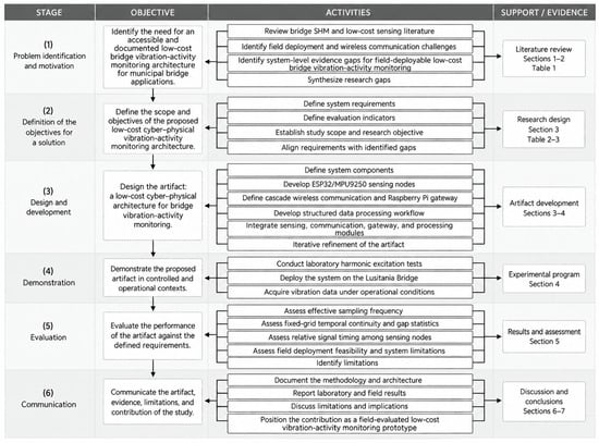
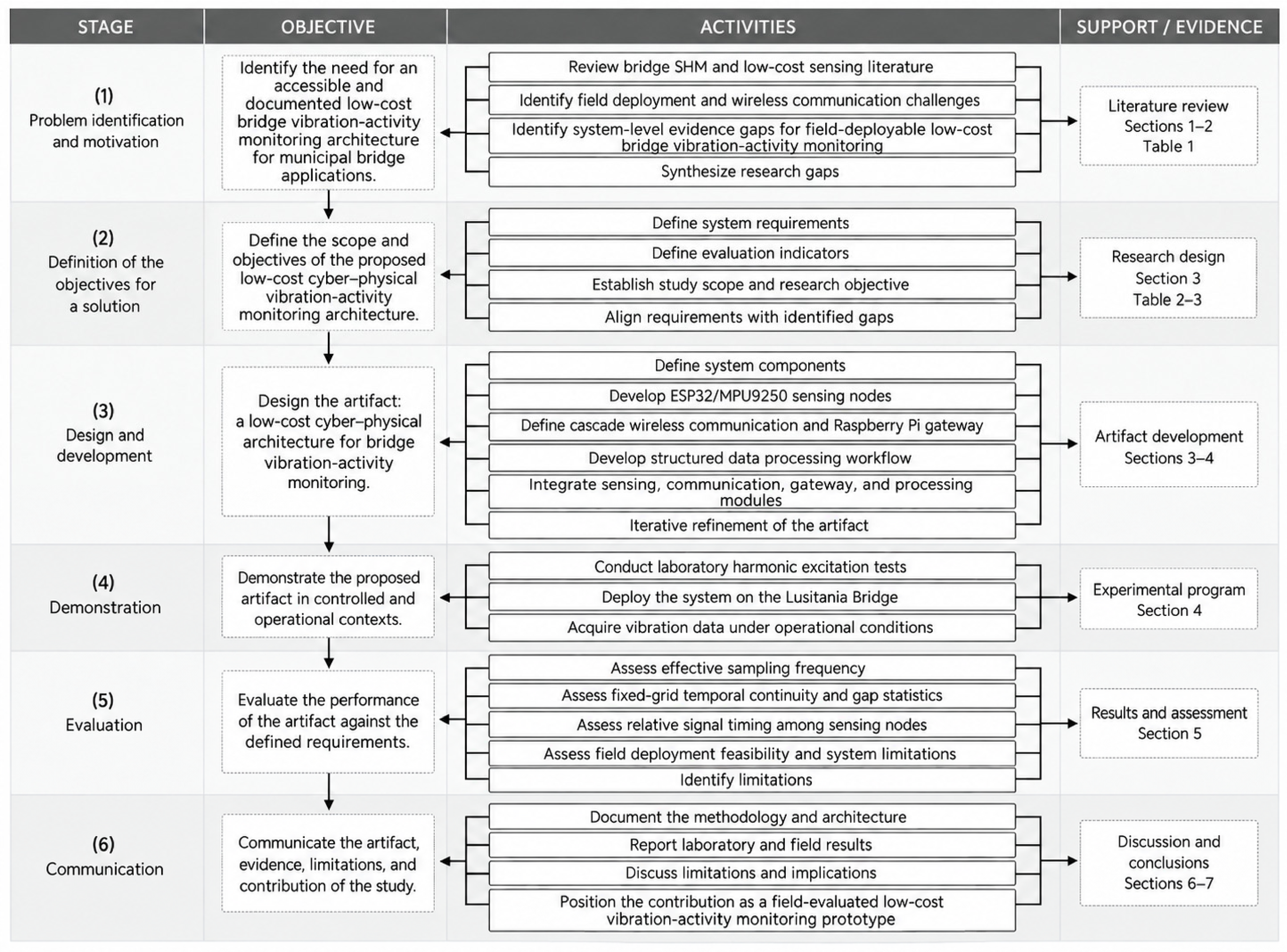
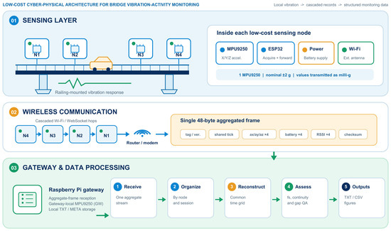
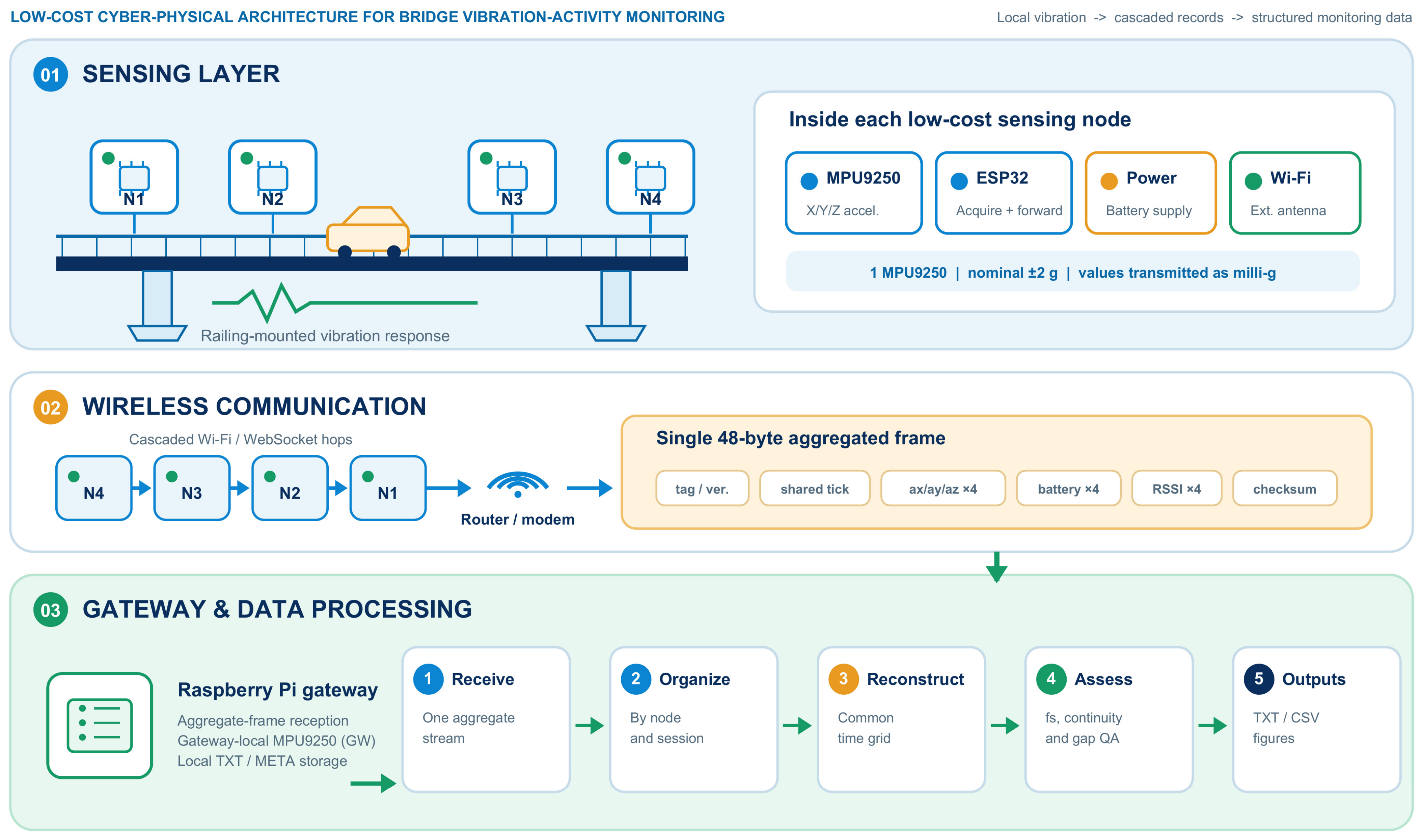
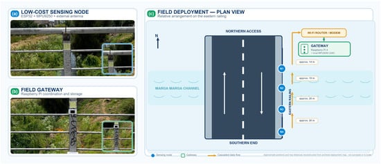
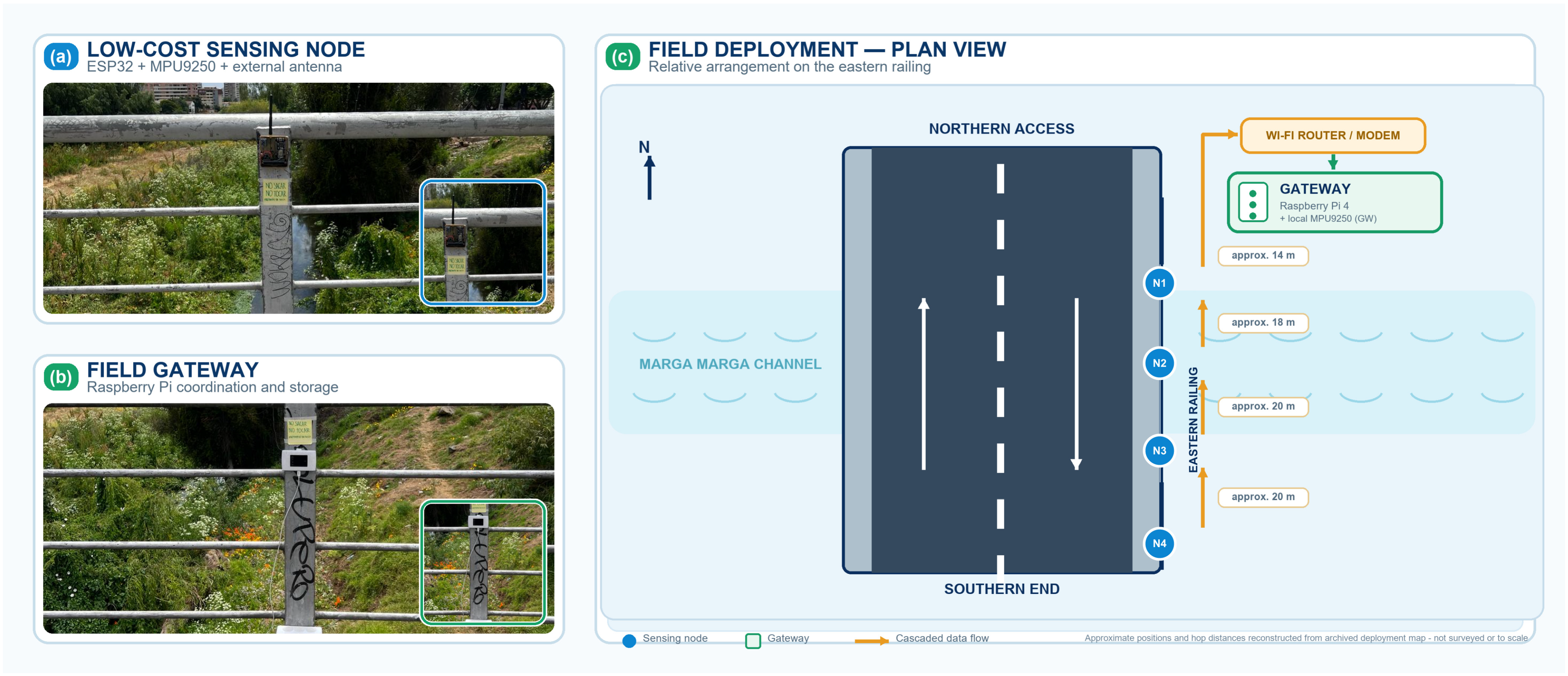
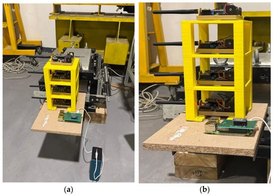
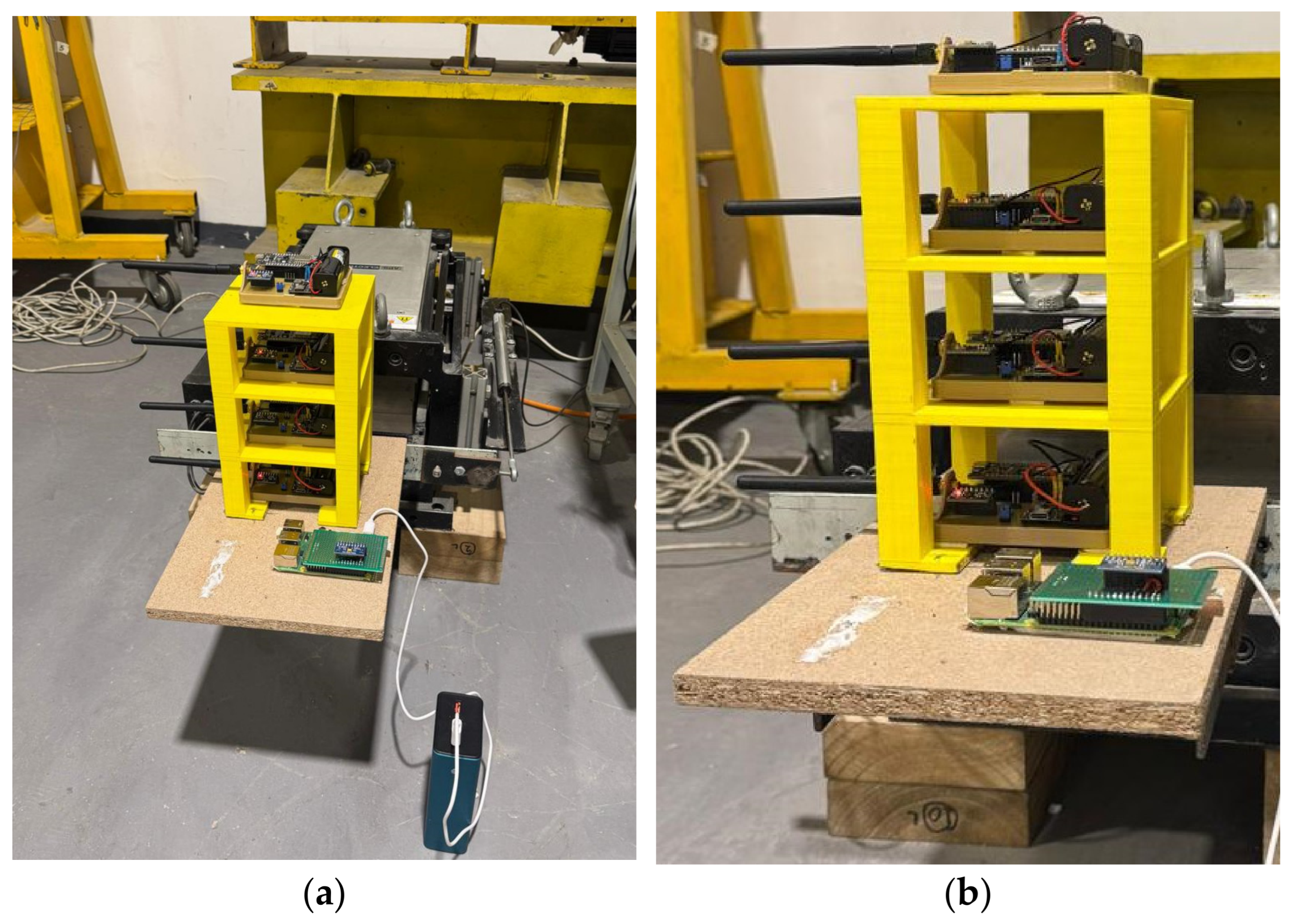
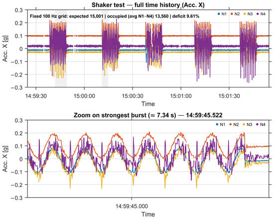
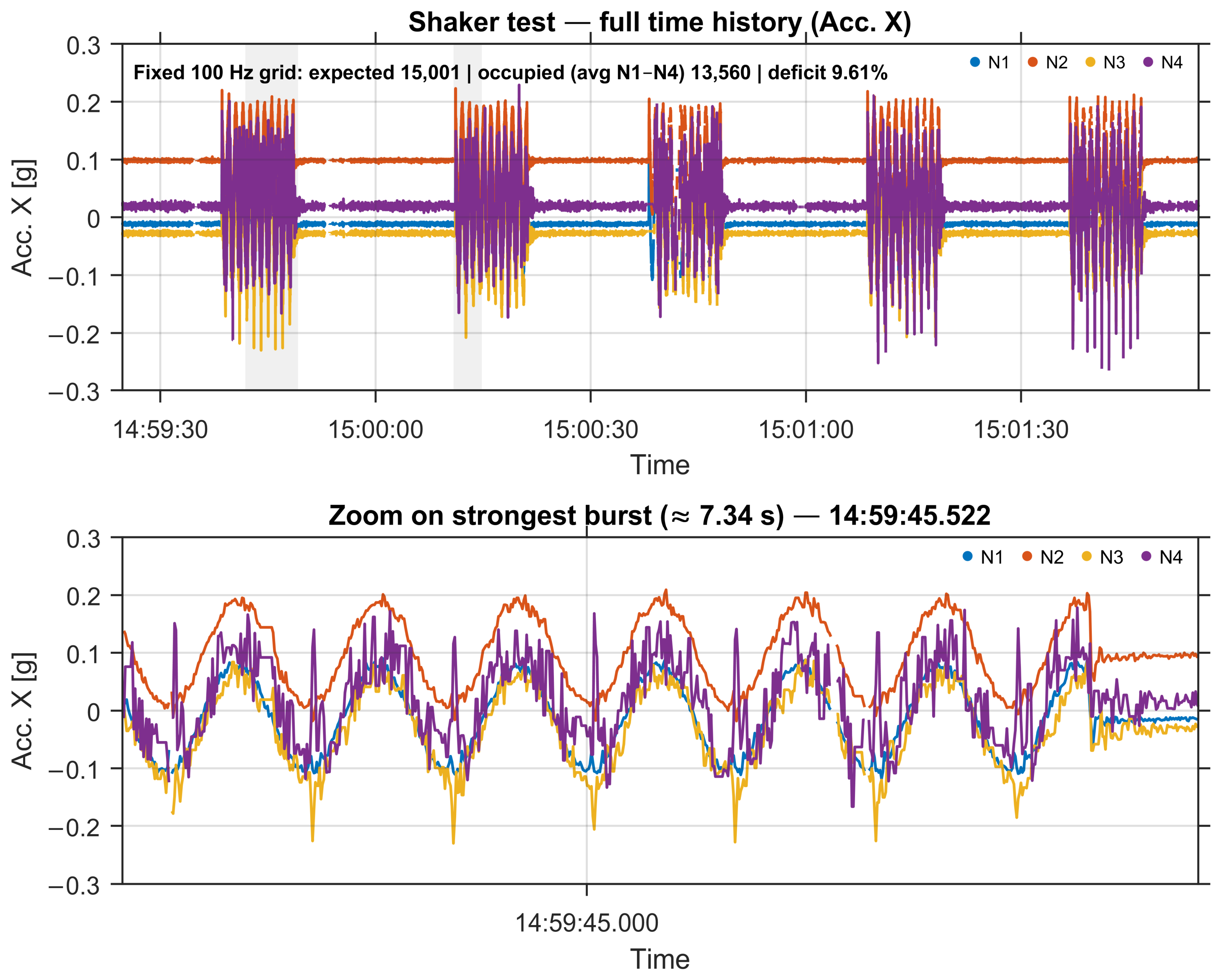
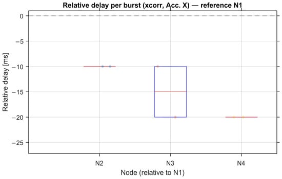
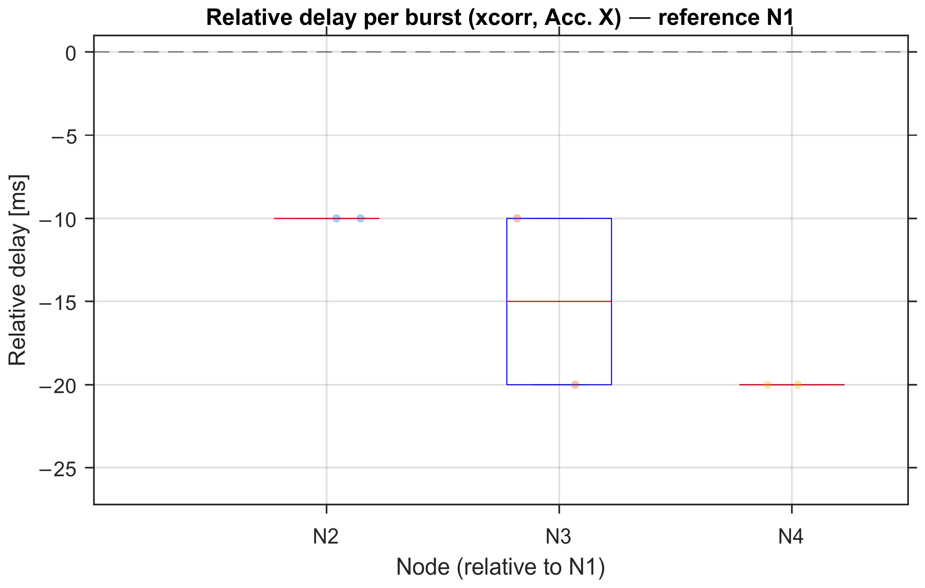
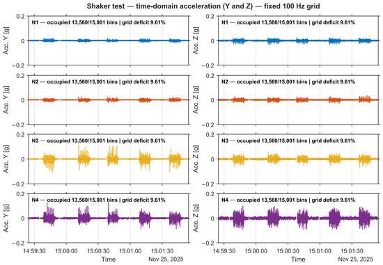
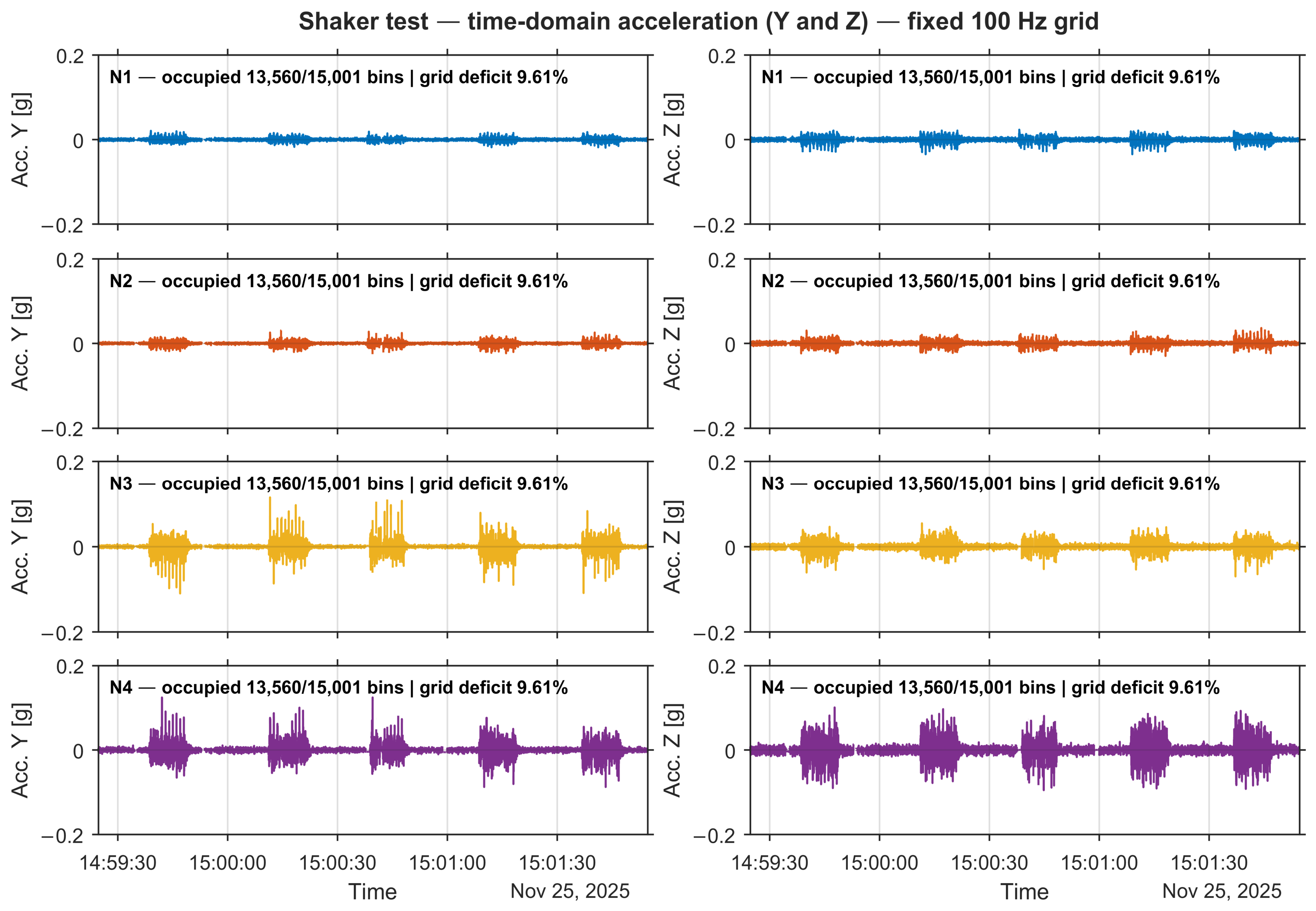
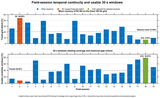
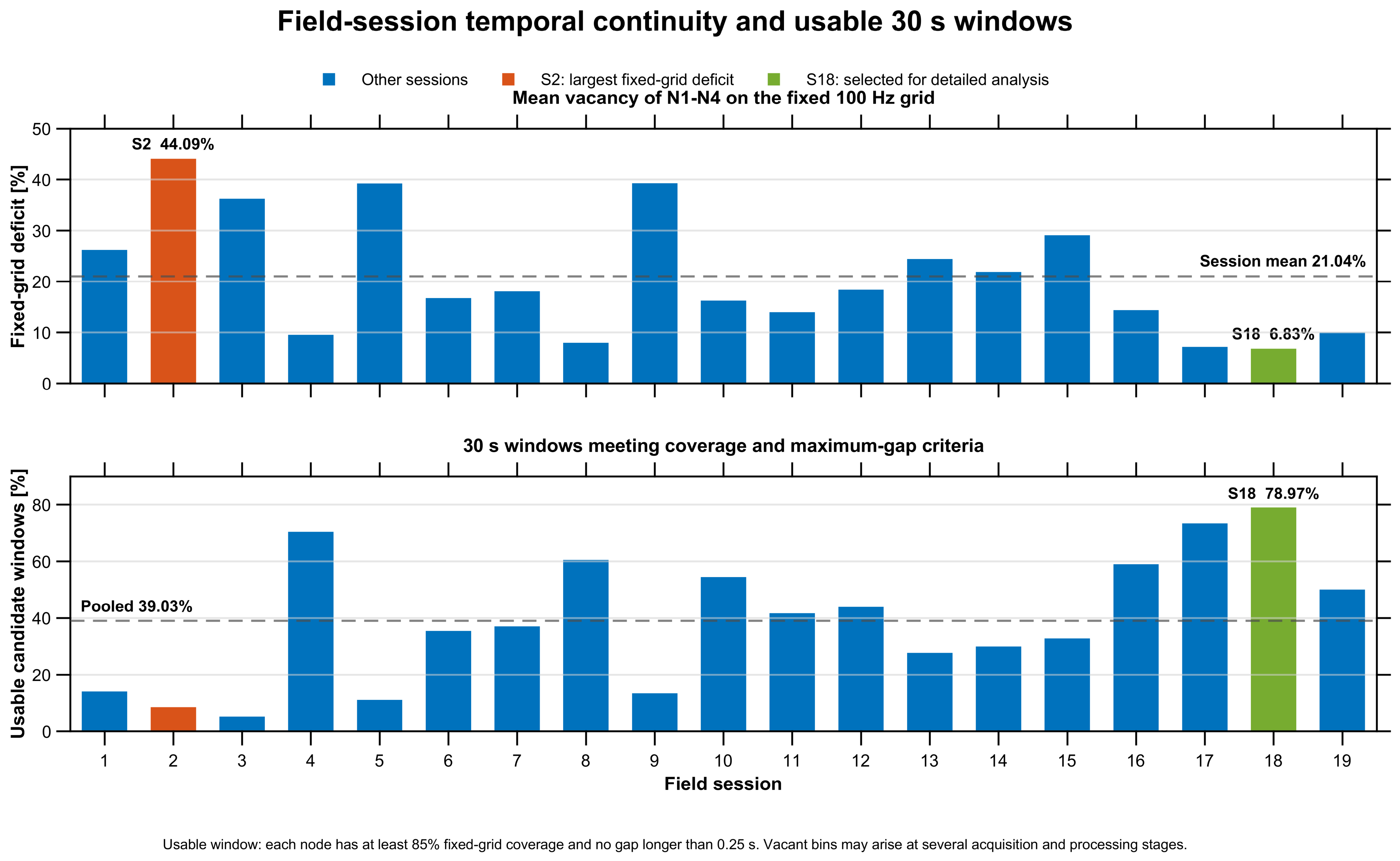
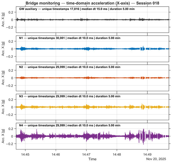
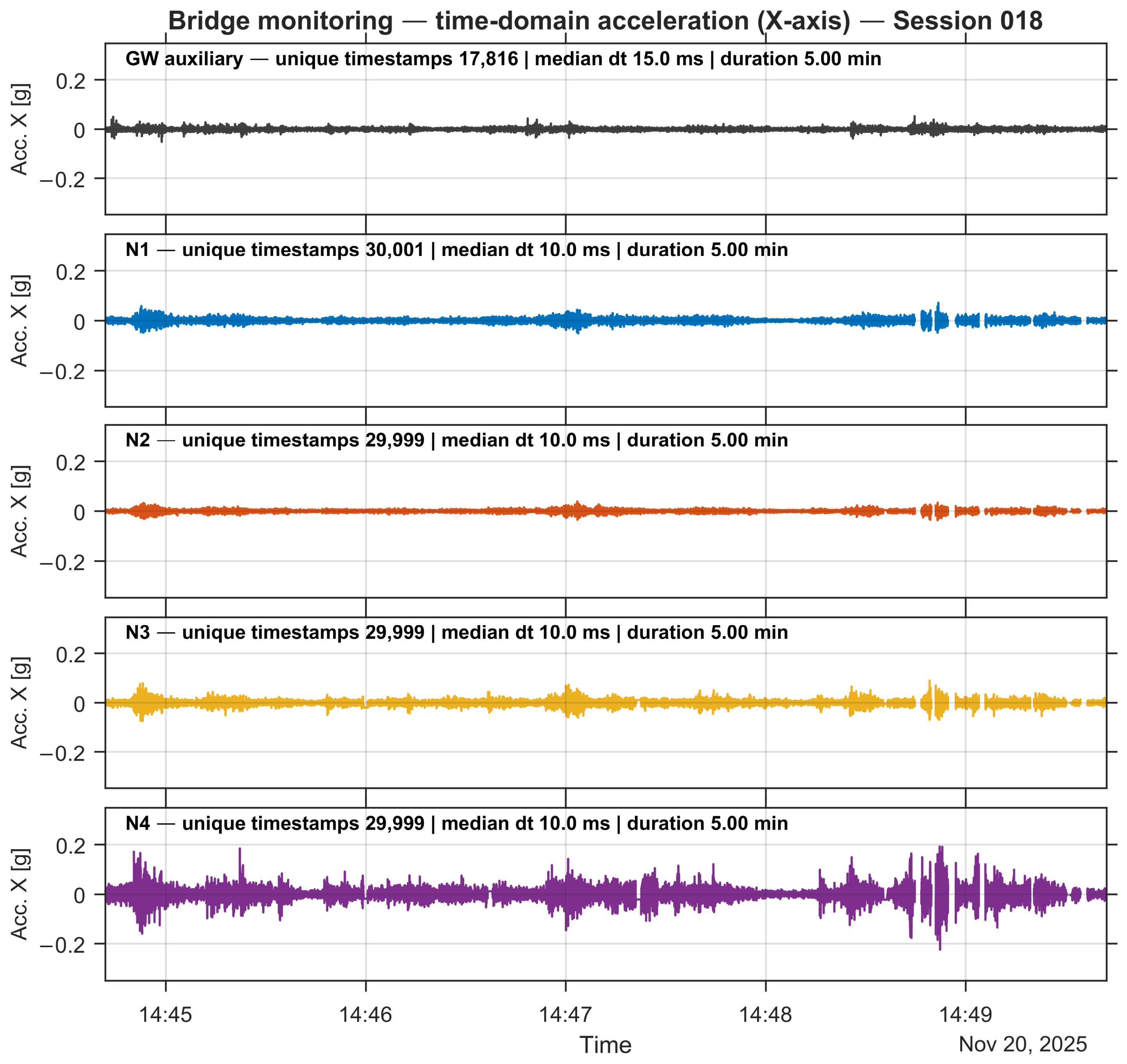
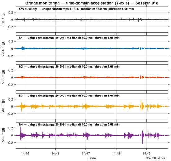
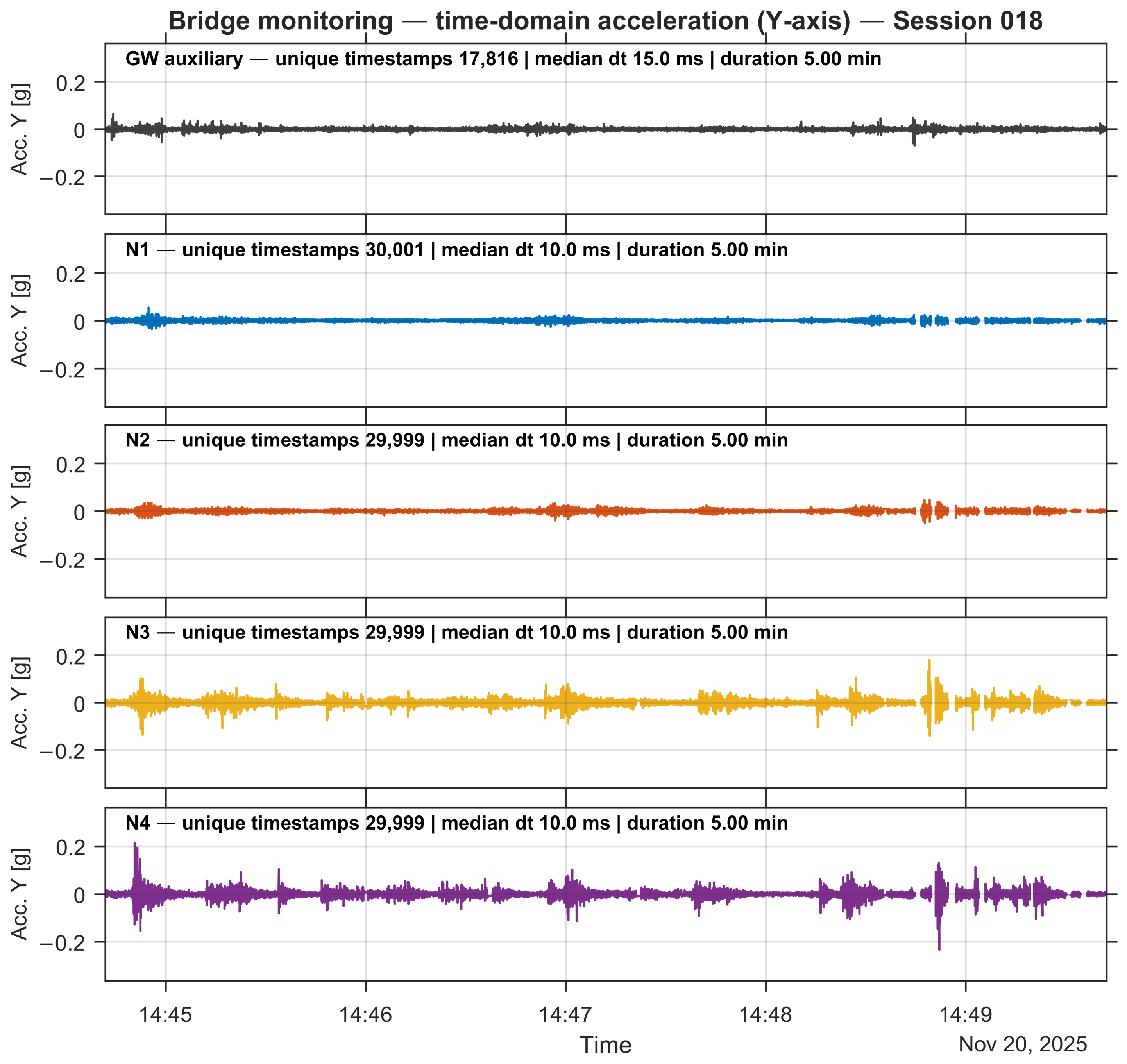
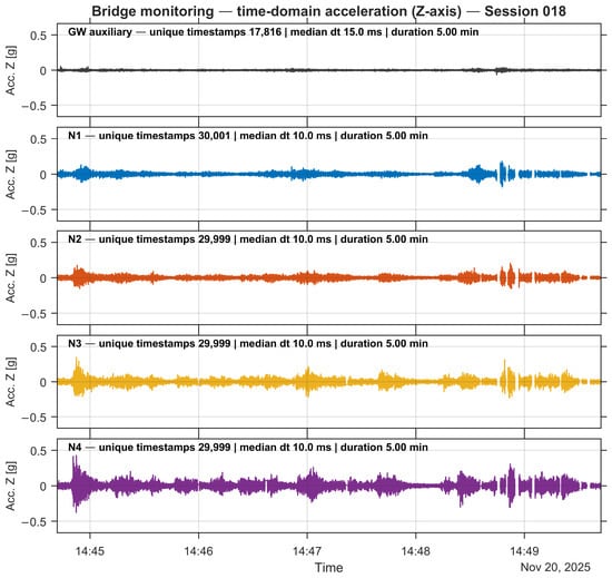
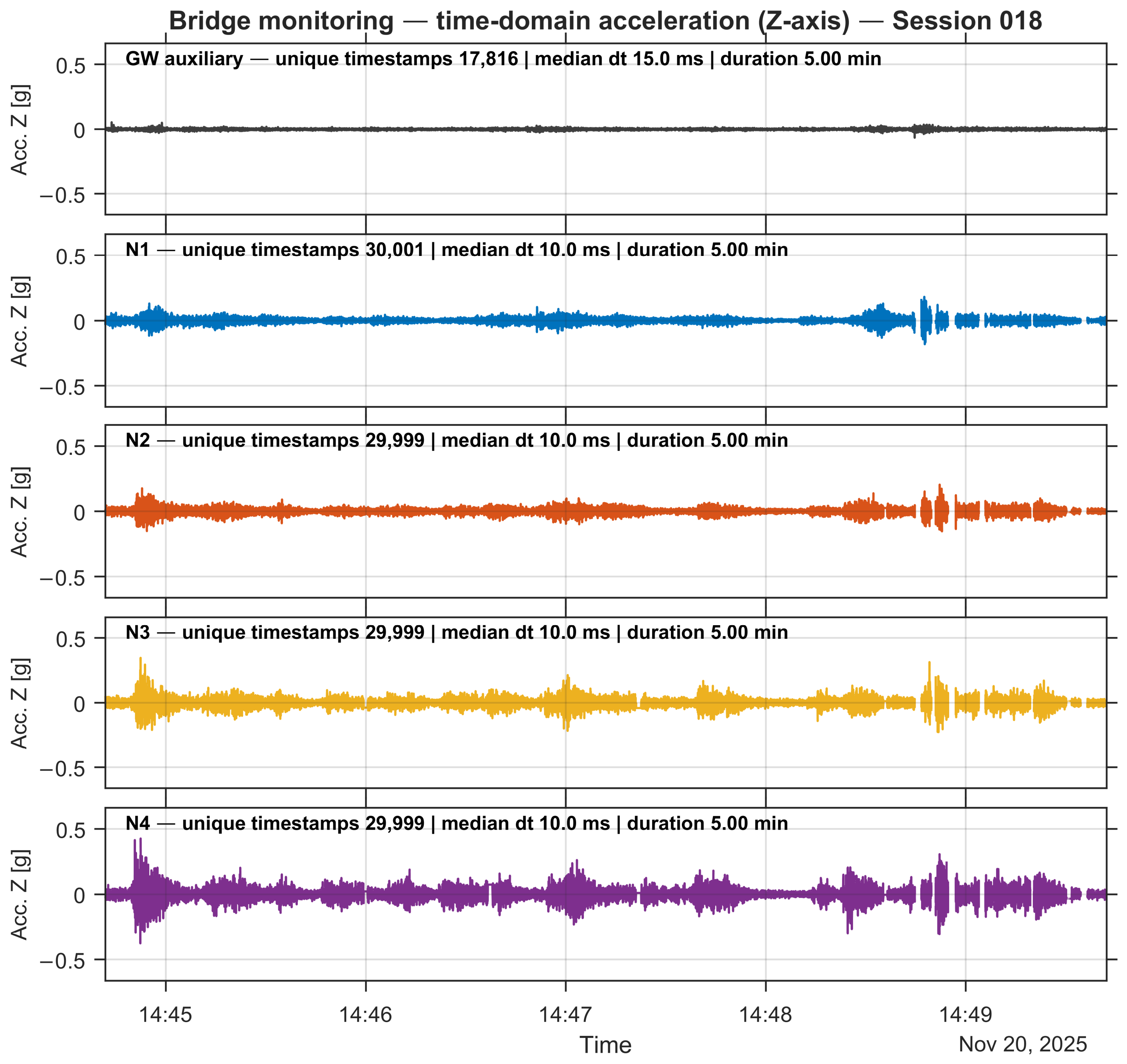
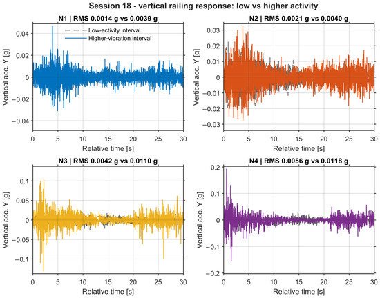
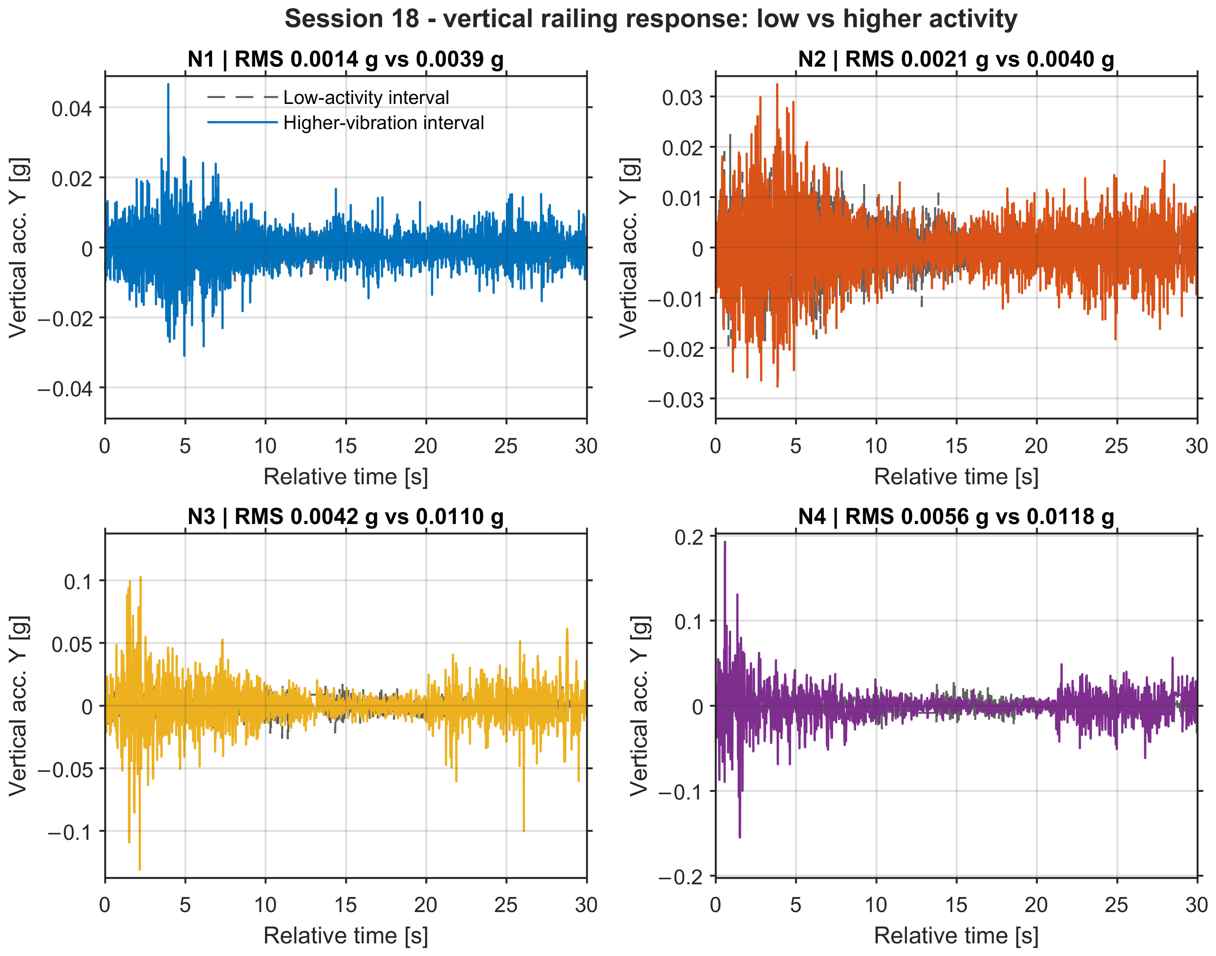
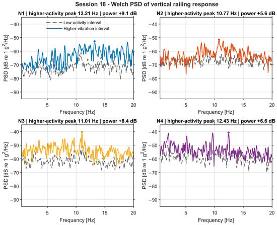
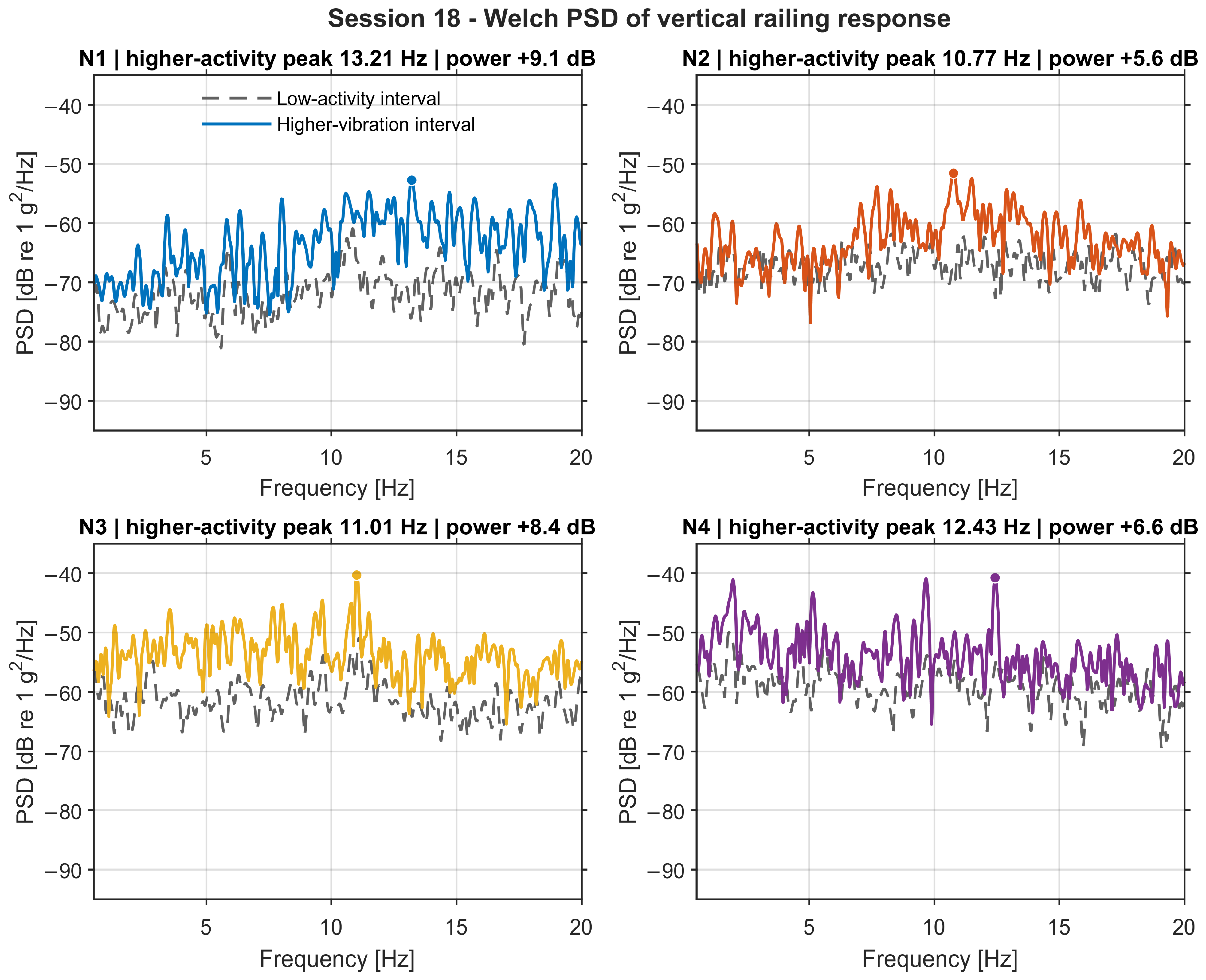

Disclaimer/Publisher’s Note: The statements, opinions and data contained in all publications are solely those of the individual author(s) and contributor(s) and not of MDPI and/or the editor(s). MDPI and/or the editor(s) disclaim responsibility for any injury to people or property resulting from any ideas, methods, instructions or products referred to in the content. |
© 2026 by the authors. Licensee MDPI, Basel, Switzerland. This article is an open access article distributed under the terms and conditions of the Creative Commons Attribution (CC BY) license.