


Highlights
Please indicate how your work links to systems science via your contributions to systems practice, theory, and/or methodology.
- Introduces a seven-block telemetry methodology that represents metaheuristic search as an observable and controllable dynamic system.
- Develops a closed-loop architecture separating stochastic LLM supervision from deterministic optimization, validation, and feasibility management.
What are the main findings and/or the implications of the main findings?
- Under a fixed 1000-iteration budget, LLM-ALNS reduced the mean gap from 2.93% for adaptive ALNS to 0.18% across nine real-road CVRPTW instances.
- Telemetry-conditioned actions improved short-budget search control while preserving feasibility, demonstrating the potential of bounded LLM supervision despite its computational overhead.
Abstract
Adaptive large neighbourhood search is steered by high-level control decisions, yet its standard adaptation reacts to a narrow reward signal that conveys little about the state of the search. Recent work has strengthened this control with machine-learning and reinforcement-learning policies, but these generally require task-specific training. This paper proposes a framework in which a large language model acts as a bounded, training-free runtime supervisor of the search. The central contribution is a structured telemetry interface that compresses the evolving search into a compact, reproducible state representation over which the model can reason. The supervisor adjusts only search-control parameters and never modifies the solution, so construction, feasibility, and objective evaluation remain inside the metaheuristic. The framework is evaluated on a multi-depot capacitated vehicle routing problem with time windows on real city street networks, against conventional variants and two dedicated solvers. Under an equal iteration budget, the supervised algorithm reduces the mean gap to the best per-instance result from 2.93% to 0.18%, and its difference from the strongest dedicated solver is not statistically significant, although it runs at a higher computational cost. These results indicate that a language model can control metaheuristic search effectively when supported by a structured interface between the algorithm and the model.
1. Introduction
An experienced practitioner watching a metaheuristic run can often tell, long before the iteration budget is spent, that something has gone wrong: operators have stopped contributing, the acceptance rate has collapsed, the search keeps revisiting the same regions, or the incumbent has not improved for hundreds of iterations. Adaptive large neighbourhood search (ALNS) makes such control decisions automatically, choosing which operators to emphasise, how aggressively to perturb, how much worsening to accept, and when to diversify [1,2]. Its standard mechanism, however, reacts to a single narrow signal, recent operator rewards [1,3], and cannot diagnose the richer pathologies a human observer recognises. A meta-analysis finds this adaptive layer yields only a modest average gain over non-adaptive selection [4], pointing to the controller’s limited view rather than to adaptation itself [5,6].
A natural response is to widen what the controller sees and to learn the policy. Reinforcement-learning controllers do this for ALNS, mapping a search-state representation to operator, parameter, and acceptance decisions [7,8], including routing with time windows [9]; each, however, needs task-specific training, engineered rewards, and re-validation when the instance distribution shifts [10]. Whether a general-purpose reasoner can make these decisions without training is therefore an open question. A large language model (LLM) is a natural candidate, since it requires no task-specific training and reasons over heterogeneous, mixed-type state indicators.
Hyper-heuristics offer a template for such supervision: a high-level strategy observes the state of the search and selects, configures, or sequences low-level heuristics without ever manipulating the solution itself [11], and this separation is what makes supervision safe. Most LLM-for-optimisation work departs from the template and uses the LLM to generate or configure solutions directly, from programmes [12] to the automated design of heuristics and metaheuristics [13,14,15,16]. Under hard constraints, this invites infeasibility and weak reproducibility, and on network-structured problems LLMs frequently violate constraints and need error correction [17]. This paper adopts the opposite division of labour: the LLM occupies the high-level role of the hyper-heuristic controller and never sees or edits the solution, while ALNS builds routes, enforces feasibility, and evaluates cost.
The central hypothesis is that effective LLM supervision depends less on the model than on how the search state is represented to it. We therefore propose a structured telemetry interface that compresses thousands of raw per-iteration events into a compact, mathematically defined, reproducible state representation, turning an opaque event stream into segment-level indicators that make stagnation, operator starvation, acceptance collapse, and infeasibility pressure directly readable in a bounded format that a general-purpose reasoner can parse reliably at every decision point.
The interface is evaluated on a multi-depot capacitated vehicle routing problem with time windows (CVRPTW) built on the real street networks of three cities, whose asymmetric, non-Euclidean travel costs give a demanding, reproducible stress test rather than a bid for best-known results. The scheme is compared against adaptive ALNS, a fixed-weight variant, and rule-based and random supervisors that read the same telemetry within the same bounds.
The research question is therefore: can a structured telemetry interface let a bounded, training-free LLM supervisor make runtime control decisions that improve ALNS under constrained dynamics? The aim is not to beat dedicated solvers on runtime, since an LLM supervisor is inherently slower, but to test whether a compact, training-free interface lets a general-purpose reasoner steer search. The paper makes the following contributions.
- A structured seven-block telemetry interface, the central contribution, that converts raw search logs into segment-level, mathematically defined indicators and thereby defines how the state of a running ALNS is represented to a general-purpose reasoner.
- A bounded LLM-supervised ALNS (LLM-ALNS) architecture in which the LLM reads only this telemetry and adjusts only search-control parameters, with a deterministic validator that checks, clips, or rejects every action before it reaches the search.
- An experimental design that isolates the effect of the decision policy, comparing LLM-ALNS against adaptive and fixed-weight ALNS and against rule-based and random supervisors that read the same telemetry within the same bounds.
The remainder of the paper is organised as follows. Section 2 reviews adaptive control in ALNS, learning-based search control, and LLMs in optimisation. Section 3 defines the optimisation problem and the supervisory-control problem. Section 4 presents the telemetry interface, the bounded intervention space, and the validation of supervisory actions. Section 5 reports the experimental design and results, and Section 6 concludes.
2. Literature Review
The CVRPTW is a widely studied constrained routing problem [18,19,20] for which exact methods guarantee optimality but scale poorly [21], classical heuristics are fast but limited in quality [22], and metaheuristics trade the optimality guarantee for high-quality solutions within practical budgets [23]. Among them, ALNS is one of the most successful routing frameworks: its destroy-and-repair design rebuilds large portions of a solution while preserving useful structure, and an adaptive rule favours operators that have recently performed well [1,2]. ALNS remains in active use for time-window variants with competitive results [24,25], so CVRPTW provides an established benchmark on which to study adaptive search control.
ALNS adaptation is driven by a narrow signal: operator scores record only recent improvement, acceptance, or rejection, and both the acceptance criterion and the operator set markedly affect performance [5,6], while the adaptive layer yields, on average, only a modest gain over non-adaptive selection [4]. Existing adaptive approaches therefore give limited visibility into the causes of stagnation or degradation, which in CVRPTW may arise from infeasible repairs, structural cycling, excessive destruction, or tight time-window structure [26,27].
Controlling an algorithm during its execution is a long-standing theme. Online parameter control adjusts an algorithm during its run [28], while offline tools such as irace tune parameters beforehand [29]. Hyper-heuristics formalise the underlying separation: a high-level strategy selecting or controlling low-level heuristics without modifying the solution directly [11], and adaptive operator selection, including bandit formulations, treats operator choice as a state-dependent decision [30,31,32]. Common to all is a representation of the search state, expressed as operator-reward histories, landscape descriptors, or hand-designed features; the design of that representation, more than the control rule alone, is the concern of this paper.
Reinforcement learning (RL) has made this representation richer, and the control policy has been learned. Surveys of machine-learning-assisted metaheuristics and of RL for combinatorial optimisation document learned policies for operator choice, parameter adaptation, and broader search behaviour [33,34,35], and neural large neighbourhood search embeds learning within the LNS procedure [36]. For ALNS specifically, deep-RL, graph-RL, and proximal-policy-optimisation controllers select operators, set parameters, and adjust acceptance and termination from learned search-state or graph encodings [7,8,9], including an electric-routing variant that draws features from the instance and the evolving solution [10], while offline RL has learned dispatching policies from historical data [37]. Learned online control of ALNS is therefore effective, at the cost of task-specific offline training, reward engineering, and re-validation of transfer when the instance distribution changes [38,39].
LLMs have entered optimisation along two lines. In the first, the LLM generates artefacts, from programmes [12] to entire metaheuristics [13,14,15,16]; used as a direct solver of network-structured problems, it frequently violates constraints and needs error correction [17]. In the second, it acts as a reasoning agent that observes a state and decides rather than producing a solution, as in the literature on LLM-based autonomous agents and controllers [40], and reasons over structured, non-textual input in tasks such as data wrangling [41]. This work belongs to the second line and differs from using an LLM as an offline tuner or configurator [42,43,44]: here, it is an online controller reasoning over a structured representation of search dynamics.
These lines locate the contribution. Existing approaches occupy two extremes: reward-based adaptation with limited state awareness, and learning-based control that achieves richer awareness at the cost of offline training. We investigate a third option: a pre-trained LLM as a training-free runtime supervisor over a structured telemetry representation of search dynamics. Because telemetry is a shared interface, the identical state can drive an LLM, a rule-based, or a random policy, which makes the LLM’s contribution, as distinct from the interface, directly testable. Table 1 summarises these control paradigms.
Table 1.
Control paradigms for ALNS-style search: The search-state signal each uses, where feasibility is enforced, and the associated reproducibility risk.
3. Problem Description
This section defines the optimisation problem (Section 3.1), casts its runtime control as a supervisory-control problem (Section 3.2), and states the hypotheses (Section 3.3). The former is the benchmark; the latter is the object of study.
3.1. The CVRPTW Optimisation Problem
We consider a multi-depot capacitated vehicle routing problem with time windows on a directed graph . The node set comprises depots and customers , and each arc carries a travel distance and a travel time . Costs are asymmetric, with in general. A homogeneous fleet of vehicles, each of capacity , serves the customers. Every vehicle is assigned to a depot, and each route starts and ends at that depot. Each customer has a demand , a service duration , and a time window within which service must begin, with waiting permitted before . The number of depots is part of the instance data, and the supervision method is independent of it.
Let equal one if vehicle traverses arc , and let be the service-start time of vehicle at node . The problem is
subject to
Objective (1) minimises the total travel distance over all vehicles. Constraint (2) assigns every customer to exactly one vehicle. Constraint (3) enforces flow conservation, so each vehicle enters and leaves every node it visits. Constraint (4) restricts each vehicle to at most one route rooted at a single depot. Constraint (5) enforces the vehicle capacity limit. Constraint (6) propagates service-start times along traversed arcs, accounting for service duration and travel time, and is linearised with a big-M constant. Constraint (7) requires service at each customer to begin within its time window. Capacity and time windows are hard constraints, so every reported solution is feasible. The fleet size is fixed and identical across all compared methods, so comparisons are not confounded by fleet size.
3.2. The Supervisory-Control Problem
The object of study is the runtime control of the metaheuristic, cast as a discrete-time problem layered above ALNS. The search advances in segments of iterations; at each segment boundary a supervisor observes the search and may adjust its control parameters, while construction, repair, feasibility, and evaluation remain internal to ALNS. The problem is defined by four objects.
- Observation space . At boundary the supervisor receives an observation , a structured telemetry vector that summarises the search state (Section 4.2). It excludes the solution: routes, coordinates, and the distance matrix are never exposed.
- Action space . An action is a bounded parameter-level adjustment, comprising a regime label and bounded changes to the destroy degree, operator emphasis, acceptance temperature and cooling, and diversification timing.
- Validator . A deterministic operator that projects any proposed action onto the admissible set, clipping out-of-range values and rejecting malformed ones, so that no supervisor output can drive ALNS into an invalid state.
- Supervisory policy . The controller maps an observation to an action, interchangeable across an LLM, a rule-based, and a random policy over identical observations and actions.
Writing for the incumbent solution and for the control-parameter vector, the closed loop is, for ,
The supervisor therefore acts only in parameter space, while construction, evaluation, and feasibility remain internal to ALNS. This hyper-heuristic separation makes the supervisory policy, not any particular language model, the unit of study.
3.3. Research Hypotheses
Let denote final solution quality, measured as total travel distance under a fixed iteration budget. The paper tests two hypotheses.
- H1 (control quality). Under an equal budget, an LLM policy that observes the telemetry and adjusts only attains better than reward-based adaptive ALNS and than rule-based and random policies operating over the same and .
- H2 (source of improvement). Any observed improvement is associated with state-aware control rather than solution manipulation. Only the second part is testable by construction: the policy never edits the solution, and a rule-based policy with identical observations isolates the decision rule from the interface. This establishes the necessary condition that the supervisor does not alter the solution, not the sufficient condition that the telemetry causes the improvement; alternative mechanisms, such as pre-training priors or beneficial stochasticity from bounded perturbations, are not excluded by the design and are noted among the limitations in Section 6.
Improvement is assessed primarily by solution quality (gap to the best per-instance result) and secondarily by convergence speed and recovery from stagnation, operationalised in Section 5.
4. Methodology
This section presents the framework components and their interaction: the baseline ALNS (Section 4.1), the telemetry aggregator (Section 4.2), the LLM supervisor (Section 4.3), and the safety validator (Section 4.4). The components run as a closed loop over segments of L iterations, so control is exercised at fixed checkpoints rather than continuously. Running a full segment before each query keeps the search efficient, with one query per segment, gives the telemetry enough events to be statistically meaningful, and bounds inference cost. The final segment runs without a query, as there is no later segment to control. Figure 1 shows the architecture and the data circulating around the loop.
Figure 1.
The supervised control loop connecting the ALNS solver, telemetry aggregator, LLM supervisor, and safety validator.
4.1. Baseline ALNS
The baseline is a standard ALNS on the open-source alns library [45] with an added segment-level control loop. Components follow established ALNS practice except for the telemetry aggregator (Section 4.2), the LLM supervisor (Section 4.3), and the safety validator (Section 4.4). All variants in Section 5.1 share the operator pool, acceptance criterion, stopping condition, objective, and seeds, so only the control policy differs.
Initial solution. A feasible start is built by greedy insertion, placing each customer at its cheapest feasible position across the available depot routes.
Destroy operators. The destroy pool comprises random, worst, and related (Shaw) removal, which removes customers similar in location and time [1], plus route, string, and time-window-cluster removal targeting temporally tight customers [46].
Repair operators. The repair pool comprises greedy insertion and regret-2 insertion, with a time-window-aware regret-3 insertion; the regret heuristics follow Ropke and Pisinger [1,46].
Local search. No separate local-search phase is used; improvement comes entirely from the destroy-and-repair cycle [1].
Adaptive operator weights. A roulette-wheel scheme updates operator weights from segment rewards [1]: the largest reward for a new global best, smaller for improving and accepted non-improving moves, none for rejected, with reaction-factor smoothing and credit assignment following Fialho et al. [3]. Because this layer is only modestly effective on its own [4], it is the limitation that the telemetry of Section 4.2 addresses.
Acceptance criterion. Candidates are accepted by simulated annealing (SA) [47], with an initial temperature of 5000 and geometric cooling of about 0.985, following the acceptance-criterion comparison of Santini et al. [5].
Stopping condition. Each run uses a fixed iteration budget.
Objective. The objective minimises total travel distance; capacity and time-window violations are penalised during the search to keep the neighbourhood connected, while reported solutions are feasible.
Random seeds. All stochastic choices draw from a single seeded generator; each configuration runs from several seeds, with the seed recorded per run.
4.2. Telemetry Aggregator
The telemetry aggregator is the central contribution of this framework: it defines how the state of the running search is represented to the supervisor. At each segment boundary, that is, every ALNS iteration, it maps the raw per-iteration log to a fixed-length, mathematically defined observation organised into seven blocks. The blocks answer, in order, four questions any runtime controller must resolve: whether the search is still progressing, why it is or is not, whether an apparent stall is real, and how much budget and constraint headroom remain. The solution itself, the routes, coordinates, and distance matrix, is never part of . Table 2 names the blocks and relates each to the state descriptors used in adaptive operator selection and reinforcement-learning control; Appendix A gives the full definition of every indicator.
Table 2.
The seven telemetry blocks, the search phenomenon each captures, and its analogue in adaptive and reinforcement-learning search control.
Figure 2 illustrates this transformation: a log of thousands of per-iteration events, impractical to transmit at every checkpoint and ambiguous for an LLM to parse, becomes a stable, low-dimensional, reproducible view of the search state. The blocks are described below, with names matching the implemented packet.
Figure 2.
The telemetry aggregator converts the raw per-iteration log into a compact seven-block packet. Each block summarises a distinct diagnostic aspect of the search before the packet is provided to the LLM supervisor.
Search dynamics (Block 1).
This block reports whether the search is still improving and how acceptance is set: current and best objective, improvement velocity over a short and a longer window, iterations since the last best, and the acceptance rate. The two velocities are the core signal, both near zero meaning a stall, and a near-zero short with a still-positive longer reading a recent slowdown, while the acceptance rate shows whether the simulated-annealing temperature is too strict or too loose. Block 1 is the primary trigger: it flags that attention is needed but not what, and the other blocks supply the diagnosis.
Operator effectiveness (Block 2).
Standard ALNS shifts weight toward recently successful operators, but the weights do not reveal when the pool is unhealthy. This block reports, per operator, how often it is chosen and how often it yields an improvement or accepted move, the evenness of selection across the pool, and a counter flagging operators ignored for several segments. When Block 1 shows stagnation, Block 2 distinguishes over-commitment to a few operators from a starving productive operator; the remedy, rebalancing operator emphasis, differs from changing how aggressively the search perturbs the solution.
Destroy/repair calibration (Block 3).
The destroy degree, the number of customers removed and reinserted per step, balances local refinement against diversification: small removals are safe and local, large removals explore more but are harder to repair feasibly. This block reports how well each operator performs at different removal sizes, in improvement and in feasible-and-accepted rate. Its role is protective: if large removals are already failing to repair, increasing the degree in response to stagnation would make the search worse, and Block 3 lets the supervisor see this before acting.
Search movement (Block 4).
A flat objective curve is ambiguous: the search may be crossing a wide region of similar-cost solutions, which is healthy, or circling the same few structures, which is not. This block separates them by measuring how much route structure changes and how often the search revisits solutions already seen; great structural change with little cost change indicates productive plateau movement, frequent revisits with little structural change indicate cycling. This refines Block 1: the same near-zero progress reading calls for patience in the first case and aggressive diversification, or a restart, in the second.
Constraint stress (Block 5).
In CVRPTW, a solution can look good on distance yet sit on the edge of infeasibility. This block measures that pressure: how close routes are to capacity, how much slack remains before time windows are violated, and whether recent repairs fail mainly because constraints cannot be met. Since improving the objective and improving feasibility are different goals, if repairs keep returning infeasible, the supervisor should ease pressure on tightly constrained solutions rather than explore harder. Block 5 keeps the decision honest about why the search is failing.
Run context (Block 6).
The same signals should not always trigger the same action: aggressive diversification is sensible early, when budget can recover, but risky late, when good structure should be protected. This block makes the supervisor budget-aware by reporting the phase, early, middle, or late, of the iteration budget, with basic fleet context; it conditions every other reading, so a late stagnation signal is treated more cautiously than the same signal early on.
Memory and governance (Block 7).
The final block closes the loop. After each intervention, it records whether the next segment improved, stayed flat, or worsened, the LLM’s stated confidence, and whether the validator scaled or rejected the action, with a counter for consecutive no-effect interventions. This gives the supervisor a short memory of its own track record and gives the validator evidence to discount low-confidence or repeatedly ineffective recommendations. Block 7 is the governance layer, holding the LLM accountable to recent outcomes.
Together, the seven blocks give a compact, consistent picture: whether progress has stalled, why, whether the stall is real, how much feasibility and budget headroom remain, and whether the last action helped. Every entry is an aggregated number or categorical flag.
4.3. LLM Supervisor
The supervisor is an LLM consulted once per segment; it instantiates the supervisory policy of Section 3.2, mapping the telemetry observation to a bounded action , and nothing else in the framework depends on the policy being an LLM rather than another controller. Its inputs, outputs, and settings are fixed for all runs so that the layer is reproducible, since the output of an LLM is sensitive to the LLM, the decoding settings, and the prompt [48]. The structure of the supervisor is shown in Figure 3.
Figure 3.
The LLM supervisor: the seven-block telemetry packet is merged into the fixed system prompt and sent to the LLM, which analyses it and returns a JSON action that the safety validator then checks.
Prompt structure. A fixed system prompt carries the supervisor role (it never edits the solution), every telemetry field’s definition, the permitted actions with their bounds, and the output schema; the seven-block telemetry is serialised as one compact JSON object and appended as the user message. State is passed as structured JSON, so the LLM reads named fields and its reply parses deterministically.
Prompt contents and interpretation rules. Beyond role and schema, the prompt fixes the action bounds, for example, operator bias in [−0.15, +0.15], a destroy degree clamped to [1, x · n] with a destroy-fraction cap (x = 0.2, chosen by preliminary trial), and a bounded acceptance-temperature multiplier. It gives eight interpretation rules covering improvement velocity, the acceptance threshold, the neutrality-ratio band, cycling versus revisiting, phase acceptance floors, the governance counters, q-stagnation diagnostics, and accepted-drift detection. Each maps a telemetry pattern to one of the same intensify, diversify, or rotate, and escape regimes as the rule-based comparator, so the two share a control vocabulary and differ only in how flexibly they apply it. The interpretation rules provide domain-specific guidance rather than a complete deterministic action policy; the LLM remains responsible for integrating the telemetry blocks and selecting a context-dependent joint control action. The full prompt is in Appendix B.
Action schema and output. The supervisor returns strict JSON: a regime label and bounded changes to the destroy degree, operator emphasis, acceptance temperature and cooling, and the timing of diversification or restart, plus a self-reported confidence in [0, 1]. No free text, routes, or customer sequences are permitted.
Model and decoding. The supervisor is OpenAI’s open-weight gpt-oss-120b model, served through Ollama Cloud and used consistently in every run. The model was invoked using the Ollama identifier gpt-oss:120b, corresponding to the fixed artefact digest a951a23b46a1 and an artefact size of 65 GB. It uses a mixture-of-experts architecture with 117 B total parameters, 5.1 B active parameters per token, and native MXFP4 quantization. Decoding was fixed at a temperature of 0.1 with nucleus sampling, a 40,000-token generation limit, and a 60 s timeout. The fixed artefact digest identifies the exact model weights used across the experiments. Although stochastic decoding may prevent bit-for-bit reproduction of individual responses, the released prompt, telemetry schema, inference settings, validator rules, random seeds, and logged supervisory decisions support reproduction and auditing of the experimental procedure.
Frequency and retry. The supervisor is consulted once per segment of L iterations, and the final segment is not sent. If the output is invalid JSON or violates the schema, it is queried once more with the same packet; if it still fails, the validator applies the fallback no-change action.
4.4. Safety Validator
The validator is a deterministic layer between the supervisor and ALNS that guarantees bounded interventions and keeps feasibility owned by ALNS. It is necessary because an LLM’s output is non-deterministic and, without guards, can produce constraint-violating actions [17,48]. A deterministic check ensures no model output can place the solver in an invalid state, preserving the hyper-heuristic separation of high-level control from low-level modification [11]. Figure 4 shows the pipeline.
Figure 4.
The safety validator: Every action is parsed, clipped to normalised bounds, and confidence-gated before it can affect ALNS; the solution is never modified.
Every action passes deterministic checks. It must parse and match the JSON schema, or the no-change fallback is used. Only permitted fields are kept. Each value is clipped to its normalised range: the destroy size q is clipped to [1, x · n] at x = 0.2, so q/|C| never exceeds 0.20, and the acceptance-temperature multiplier is clipped to [0.75, 1.35]. Per-segment change is limited: operator weights are normalised to sum to one, each per-operator bias is clipped to ±0.25, and the total absolute change is capped at 0.30 for destroy and 0.25 for repair. Any field altering the solution is rejected. Finally, the action is confidence-gated: it is applied in full above 0.60, at half strength between 0.40 and 0.59, and ignored below 0.40, with weights reverting toward uniform on any failure. The self-reported confidence is used solely as an uncalibrated gating signal to attenuate or suppress actions; it is not interpreted as a calibrated probability of improvement or as a predictor of decision quality. The gate is deliberately one-sided: low confidence only attenuates or suppresses an action and never amplifies it beyond the bounds, so miscalibration can make the supervisor more cautious but never larger or unsafe.
5. Experimental Results
5.1. Experimental Design
Benchmark instances are built on the real road networks of three cities, Genoa, New York, and Valencia. Road graphs are obtained with OSMnxOSMNX 2.1.0 [49], and arc travel times and distances are computed as shortest paths over the street network with NetworkX using posted speed limits. The resulting costs are asymmetric and non-Euclidean, which reflects operational conditions more faithfully than Euclidean or randomly generated benchmarks and weakens the geometric regularities that destroy and repair operators often exploit, making the test bed more demanding [50]. For each city, we generate instances with 50, 100, and 150 customers, giving nine instances. Their parameters are summarised in Table 3. Although nine instances is a modest count, the design prioritises controlled comparison over benchmark breadth: the three cities span distinct street-network topologies, the three sizes (50, 100, 150 customers) cover small to medium CVRPTW, and every solver runs on the identical instances and seeds, so each comparison is paired and instance difficulty is held constant. The evaluation is therefore aimed at detecting consistent within-instance differences between control policies, which is the object of study, rather than at establishing absolute performance across a broad suite. Wider external validity across more networks and sizes is left to future work. The multi-depot configuration is deliberate: assigning routes across several depots increases spatial and constraint interaction and yields a more demanding control problem than a single-depot setting.
Table 3.
CVRPTW instance parameters.
Every method is run on every instance from four random seeds (42, 123, 456, and 789), and statistics are aggregated across seeds. Each run uses a budget of 1000 iterations, and the LLM supervisor is consulted every iterations, giving 19 decision checkpoints per run. The compared methods are as follows:
- Standalone ALNS with fixed equal operator weights and no adaptation.
- ALNS with standard adaptive operator weighting [1].
- Rule-based supervised ALNS: A deterministic policy over the same telemetry and bounded action space. It intensifies while the incumbent improves, diversifies after one flat segment, and escapes after several consecutive flat segments (large destroy degree near the cap, reheating, restart from the best), nudging the acceptance temperature when the acceptance rate is too low or too high. Both policies act over the same intensify/diversify/escape vocabulary and the identical telemetry and action bounds, the rule-based one applying fixed thresholds and the LLM the same regimes with context-dependent conditioning, so the comparison isolates how the decision is made rather than which control actions are available.
- Random supervised ALNS, sampling actions uniformly within the same bounds.
- LLM-supervised ALNS, the proposed method.
- External reference solvers PyVRP 0.013.4 [51] and Google OR-Tools 9.15 [52], reported to situate the ALNS family rather than as the primary comparison.
In total, solvers run on nine instances with four seeds, giving 252 runs, of which the 36 LLM-ALNS runs yield 684 logged supervisory decisions (19 checkpoints per run). All reported solutions are feasible. Because distances differ across instance sizes, quality is summarised by the gap to the lowest mean distance on each instance, where the mean is taken over the four seeded runs, the mean per-instance rank among the seven solvers (1 = best to 7, then averaged), and the number of per-instance wins. The evaluation follows the hypotheses of Section 3.3: solution quality tests H1 (Section 5.3 and Section 5.4) and supervisor behaviour tests H2 (Section 5.5 and Section 5.6).
5.2. Metrics
The final objective value alone is not sufficient for a rigorous evaluation. Search behaviour and intervention quality are therefore reported as first-class results. Table 4 lists the reported metrics, their definitions, and the reason each is included.
Table 4.
Evaluation metrics.
These metrics follow established practice for routing metaheuristics. Solution quality and the gap to a reference are the standard basis for VRP comparison [25,53]. Convergence speed and time-to-best capture anytime behaviour, which is shaped by the controls the supervisor adjusts [5]. The four seeded replications per instance guard against single-run conclusions, as emphasised by meta-analyses of stochastic search [4], with seed ranges shown in Figure 5 and Figure 6. The supervisor-specific metrics are reported because the final objective alone cannot show whether supervision, rather than chance, drives any change. The rule-based and random baselines are held to the same standard.
Figure 5.
Objective-gap distribution across the 36 runs of each solver (nine instances × four seeds; diamond = mean; lower is better). Gaps are measured to the lowest per-instance mean distance over the four seeds. For the seed-deterministic reference OR-Tools, the spread reflects differences across the nine instances, not across seeds.
Figure 6.
Convergence on the nine instances (rows = cities, columns = sizes): mean best objective over four seeds (line) with the seed range (shaded); ALNS family only.
5.3. Overall Solution Quality
Table 5 reports mean performance; lower gap, rank, and runtime are better, and wins count the instances, nine at most, on which a solver attains the best mean distance over the four seeds. The external solvers behave as expected: PyVRP is very strong and far faster (0.15% gap, rank 1.89), and OR-Tools reaches a 2.14% gap. Both are treated as competitors and are included in the omnibus and pairwise tests of this subsection. Within the ALNS family, the fixed-weight (2.86%) and adaptive (2.93%) variants trail the rule-based (1.39%) and random (1.57%) supervisors. LLM-ALNS attains the lowest ALNS-family mean gap (0.18%) and the best mean per-instance rank (1.56), with five wins, ranking first on five of the nine instances, second on three, and third on one (Figure 5 and Figure 7). Because the reference is the best result within the tested pool, and the strong external solver PyVRP anchors that pool, these gaps quantify relative standing among the compared solvers rather than proximity to a proven optimum. The random supervisor uses the identical seven-block packet and action bounds but does not condition its choices on the packet’s content, so it functions as a telemetry-blind control over the same interface. The margin between it and the two telemetry-reading policies, LLM-ALNS and the rule-based supervisor, therefore isolates the value of conditioning decisions on the telemetry content. The fact that random already improves on the adaptive and fixed-weight variants indicates that part of the gain comes from the bounded action space itself. As an external anchor, PyVRP is a peer-reviewed state-of-the-art CVRPTW solver, so the 0.03 percentage-point difference between LLM-ALNS (0.18%) and PyVRP (0.15%) places the supervised search close to a strong dedicated baseline.
Table 5.
Mean solver performance across the nine instances and four seeds. Bold marks the best value in each numeric column (lowest gap, lowest rank, most wins, shortest runtime).
Figure 7.
Solver rank on each of the nine instances (1 = best).
These differences are statistically supported. Statistical tests are conducted on per-instance means rather than on the 36 individual runs, because seeds are replicates within an instance rather than independent experimental units. Testing the per-instance means avoids pseudo-replication and keeps every comparison paired at the level of the instance. A Friedman test over the nine instances rejects the null of equal performance across the seven solvers (, ). Pairwise Wilcoxon signed-rank tests, with Holm–Bonferroni correction for the six simultaneous comparisons, show that LLM-ALNS 7.0.0 significantly improves on every ALNS variant, namely adaptive, fixed-weight, rule-based, and random ( in each case, the minimum attainable for nine paired instances, since LLM-ALNS wins on all nine, so all four survive the correction). Against OR-Tools, the uncorrected value () does not survive the correction, so this difference is not statistically significant after adjustment. The difference from PyVRP is likewise not significant (). LLM-ALNS therefore significantly outperforms the four conventional ALNS variants, whereas its differences from OR-Tools and PyVRP are not statistically significant after correction. The non-significant PyVRP result should not be read as evidence of equivalence, since a test over nine instances, even with four seeded replications per instance, has limited power to establish it, and a formal equivalence claim would require a two-one-sided-test analysis with a pre-specified margin.
5.4. Convergence and Runtime
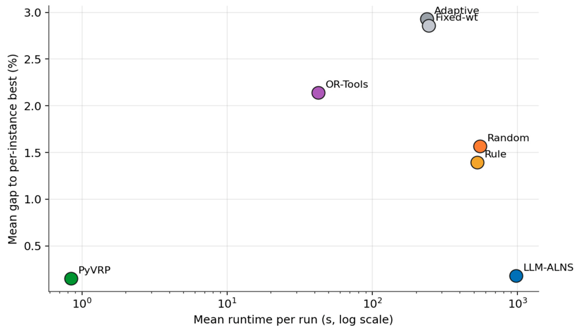
All solvers make most of their progress early. LLM-ALNS reaches its best solution at about 66% of the budget, and its longest stretch without improvement is 446 iterations, below adaptive (540), fixed-weight (516), and random (543), though the rule-based variant is shorter still at 411 (Figure 6). Supervision costs runtime (Figure 8): LLM-ALNS averages about 979 s per run against 238 s for adaptive ALNS and 0.8 s for PyVRP, with about 17 completed model calls per run. The remaining checkpoints fall back to the deterministic no-change action, for example, after a decoding timeout, and every checkpoint is logged as a decision regardless, which is why 19 logged decisions per run coexist with about 17 completed calls. Most of the overhead is telemetry instrumentation rather than the LLM calls, which account for roughly 13% of the wall-clock time.
Figure 8.
Mean runtime per run (log scale) versus average gap to the per-instance best; lower-left is better.
5.5. Supervisor Behaviour
This subsection characterises what the supervisor does across the 684 logged decisions.
Action vocabulary. The bounded action space is used in a diversification-led manner: diversify, escape, and explore together account for 450 of the 684 decisions (65.8%) and intensification for 234 (34.2%), so the supervisor defaults to neither pole (Figure 9).
Figure 9.
Bounded action vocabulary selected by the supervisor.
Telemetry coverage. The blocks contribute unevenly by design: Persistent blocks fire on almost every decision, operator effectiveness (B2) at 95.9% and constraint stress (B5) at 83.6%, with search dynamics (B1) at 68.6% and search movement (B4) at 56.1%, while event-driven blocks fire less often, memory and governance (B7) at 32.9%, destroy and repair calibration (B3) at 27.3%, and run context (B6) at 16.4% (Figure 10).
Figure 10.
Decisions in which each telemetry block surfaced an actionable signal.
Situation-conditioned regimes. The chosen regime tracks the diagnosed search situation (Table 6): Healthy states retain substantial intensification (diversification-family share 52.1%), plateau and stagnation shift the supervisor toward escape and diversification (70.7% and 70.4%), cycling is handled mainly by diversification (83.9%), and frozen simulated-annealing states are treated as full diversification territory (100%).
Table 6.
Action regimes conditioned on the diagnosed search situation. Bold marks the most frequently selected regime for each situation.
Operator-bias policy. A supervisory action also reshapes the operator-selection distribution rather than only emitting a label. The most frequent biases boost structure-aware operators, regret- insertion (525 decisions) and Shaw removal (478), while cutting greedier or less productive choices, greedy insertion (384) and worst removal (468).
5.6. Decision Quality
This subsection tests H2: that the seven-block telemetry, not the mere presence of an LLM, shapes the supervisor’s decisions across the 684 checkpoints. Each block reports a state, the model maps that state to a bounded ALNS control action, and the deterministic engine keeps feasibility, construction, and objective evaluation. We therefore ask whether the supervisor changes its action when a signal becomes active, whether it then selects the matching lever, and what the immediate effect is. All evidence is reported as percentages and percentage-point (pp) shifts, and a shift is read as a decision-conditioning effect, not as causal proof. In the absence of a controlled interface ablation, these per-block conditioning effects are the primary evidence that each block contributes distinct, actionable information to the supervisor; a degraded-interface ablation that isolates the causal contribution of individual blocks remains future work.
Table 7 reports, for each block, how often the mapped control action is selected without and with that block’s signal. The difference is the decision-conditioning effect. Every block moves the action distribution in the expected direction, and the shift is largest for the most decisive levers: when destroy/repair telemetry (B3) reports that large removals have stopped improving, q-reduction rises from 35% to 93% (+58 pp). When search movement (B4) detects cycling, diversification or operator rotation rises from 42% to 80% (+38 pp). When search dynamics (B1) reports a stagnant or frozen search, relax, reheat, or escape rises from 39% to 71% (+32 pp). The remaining blocks shift from already high baselines because their responses are partly active by default (B6 +16 pp, B2 +10 pp, B7 +10 pp, B5 +7 pp). B5 and B6 are feasibility-protection and phase-control blocks whose value is contextual control rather than a single mechanical switch. Because each mapped action is the one the prompt’s interpretation rules prescribe for the corresponding signal, Table 7 is best read as a fidelity, or prompt-compliance, audit of the interface: it confirms that the supervisor reliably operationalises the encoded rules over the telemetry, not that it independently infers these mappings.
Table 7.
Telemetry-conditioned decision shift: the rate at which the supervisor selects each block’s mapped control action without and with that block’s actionable signal (in percentage points). Computed over the 684 logged LLM-ALNS decisions (36 runs). Bold marks the decision-conditioning shifts of at least 30 percentage points.
Beyond changing the action distribution, signal-to-control fidelity asks whether, when a signal is active, the supervisor usually selects the corresponding lever. The high-leverage signals show near-complete fidelity: cycling leads to diversification or rotation, a neutral plateau to escape or reset, operator imbalance to operator movement, and constraint stress to repair-safe protection. This is the practical meaning of a useful telemetry interface: it does not merely describe the search; it directs the supervisor to the correct bounded control lever.
The decisions are also state-appropriate (Table 8). A decision counts as matching when the selected action is the response the interpretation rules prescribe for the diagnosed state: a diversification-family action for plateau, stagnation, and cycling; intensification for healthy states; and reheating or continued refinement for frozen states. Late-phase intensification without increasing the destroy size also counts as prescribed consolidation, which is why plateau and cycling reach 100% even though Table 6 records intensification decisions under both states. Under this criterion, the match rate is 100% for plateau and cycling and 70.5% in healthy states. The share of decisions improving within the next segment is high in healthy and frozen states (72.2% and 70.0%) and lower under plateau and cycling (28.4% and 32.1%), as expected, since diversification and escape position the search for later gains rather than immediate ones.
Table 8.
State-appropriate supervisory decisions: the share of decisions matching the diagnosed state, the share improving within the next segment, and the preferred control logic for each state. Shares are computed over the per-state decision counts of Table 6 (Healthy 234, Frozen SA 10, Stagnation 159, Plateau 225, Cycling 56; 684 in total). Bold marks the highest matching share. The improvement column is left unmarked, since a lower immediate improvement share under plateau and cycling reflects the deferred payoff of diversification rather than weaker decisions.
The temperature lever is the exception. When a reheat is specifically recommended, the supervisor follows it with an actual reheat in only about 30% of cases, preferring relax or escape, so the acceptance channel is the least reliably controlled. This is a genuine controller weakness and the clearest target for the next revision, either as a stronger prompt constraint or as a deterministic reheat rule inside the validator under frozen simulated-annealing conditions.
Immediate objective improvement is not the only valid outcome, since diversification and escape have deferred rather than immediate payoff: across the logged decisions, 17.8% improved the incumbent immediately, 69.9% left it unchanged, and 12.3% worsened it, a distribution consistent with a positioning role rather than greedy improvement. These rates are reported for the LLM supervisor alone; establishing supervisory effectiveness would also require the corresponding post-decision improvement rates for the random and rule-based supervisors and for unsupervised ALNS, which we identify as part of the extended analysis in Section 6.
Every decision is also safe under the validator: no audited action is hard-invalid, all parse and respect the bounded ranges of Section 4.4, and every reported solution is feasible. The cost is canonicalisation: 72.7% of actions require some soft normalisation, most often clipping the requested destroy fraction to its cap, a reproducibility consideration rather than a solver failure. The high rate, dominated by clipping the requested destroy fraction to its cap, reflects the raw model frequently proposing actions at or beyond a bound rather than structurally invalid ones; the validator’s clipping keeps them admissible, and the rate is reported for transparency about how often the bounds bind.
Taken together, the audit supports H2 in the form the evidence allows: the seven-block telemetry gives the supervisor a compact but actionable view of the search, and when high-leverage signals become active, the supervisor changes its bounded control actions by clear percentage-point margins and with high signal-to-control fidelity. The improvement is associated with state-aware decisions over a representation the supervisor reasons about, not with manipulation of a solution it never accesses. The central contribution is therefore not a universal final-distance win over every ALNS variant, but state-aware, telemetry-conditioned control that the reward-based and fixed-weight baselines cannot produce. One caveat qualifies this attribution: the rule-based comparator applies the shared intensify/diversify/escape regimes with fixed thresholds, whereas the LLM applies the same regimes with the finer, context-dependent conditioning of its eight interpretation rules, so the measured margin is an upper bound on the contribution of that conditioning relative to an equally well-specified fixed-threshold controller. Read across Table 7 and Table 8, the block-by-block decision shifts and the state-appropriate response rates give observational, not experimental, evidence that the individual telemetry blocks carry distinct and usable signal; they show that the supervisor’s actions track each block’s content, though they do not, on their own, isolate the causal contribution of any single block.
6. Conclusions
This study investigated whether a structured telemetry interface can enable a large language model to supervise ALNS without accessing or modifying the underlying solution. The proposed interface summarises the evolving search through seven telemetry blocks, while a deterministic validator restricts the LLM to bounded parameter-level actions and preserves feasibility within the ALNS solver.
The framework was evaluated on nine multi-depot CVRPTW instances derived from real road networks, using four random seeds and a fixed budget of 1000 iterations. LLM-ALNS achieved the lowest mean gap among the ALNS variants, reducing it from 2.93% for adaptive ALNS to 0.18%, and significantly outperformed the fixed-weight, adaptive, rule-based, and random ALNS variants. Its difference from PyVRP was not statistically significant, although PyVRP remained substantially faster. All reported solutions were feasible, and all supervisory actions remained within the validator’s admissible bounds. The decision analysis further showed that the supervisor changed its control actions consistently with the telemetry signals, supporting the usefulness of the interface for state-aware runtime control.
These findings are limited to the evaluated short-budget setting and should not be interpreted as evidence of general superiority over dedicated CVRPTW solvers or the broader ALNS literature. The study also used one LLM, a fixed telemetry configuration, and no individual-block ablation. By construction, the supervisory role is model-agnostic: any model that returns schema-conformant, bounded actions from the same telemetry could occupy it, but this cross-model generalisability has not been empirically tested here. Future work should therefore examine longer iteration budgets, alternative models, threshold sensitivity, and degraded or single-block telemetry configurations. Within the evaluated setting, the results demonstrate that structured telemetry can provide a practical and reproducible interface for bounded LLM supervision of metaheuristic search.
Author Contributions
Conceptualization, M.R.; methodology, M.R. and J.M.; software, M.R.; validation, J.M.; formal analysis, M.R. and J.M.; investigation, M.R.; resources, M.R. and J.M.; data curation, M.R.; writing, original draft preparation, M.R.; writing, review and editing, M.R., J.M. and F.T.; visualisation, M.R.; supervision, F.T. and J.M.; project administration, F.T.; funding acquisition, J.M. All authors have read and agreed to the published version of the manuscript.
Funding
This research received no external funding.
Institutional Review Board Statement
Not applicable.
Informed Consent Statement
Not applicable.
Data Availability Statement
The nine CVRPTW benchmark instances, the telemetry configuration file listing all threshold constants used in the experiments, and the full supervisor prompt will be deposited in a public repository (Zenodo) upon acceptance and are available from the corresponding author in the meantime. The released environment specification records the OSMnx and NetworkX versions and the OpenStreetMap extract dates used to build the instances, together with the customer-sampling and depot-placement procedures, so that the instances can be reconstructed deterministically from the four random seeds.
Acknowledgments
During the preparation of this manuscript, the author(s) used a large language model (the system under study) as a runtime search supervisor as described in the Methodology; no generative AI tool was used to write the scientific text beyond minor language editing. The authors have reviewed and edited all content and take full responsibility for the publication.
Conflicts of Interest
The authors declare no conflicts of interest.
Abbreviations
The following abbreviations are used in this manuscript:
| ALNS | Adaptive Large Neighbourhood Search |
| CVRPTW | Capacitated Vehicle Routing Problem with Time Windows |
| VRP | Vehicle Routing Problem |
| LLM | Large Language Model |
| RL | Reinforcement Learning |
| JSON | JavaScript Object Notation |
| CV | Coefficient of Variation |
Appendix A. Telemetry Indicator Definitions
This appendix collects the formal definitions of the telemetry indicators described in Section 4.2. The notation, the seven blocks, and the equation for every indicator are reproduced here exactly as implemented; Section 4.2 gives the plain-language account of what each block measures and why. The numerical values of every threshold constant appearing in these definitions are listed in the telemetry configuration file released with the paper (see the Data Availability Statement), so that each block indicator can be recomputed exactly from raw ALNS logs.
Notation. The symbols used throughout this section are listed below. Computed indicators are defined in the block tables that follow; the table here collects the input quantities, indices, and constants that appear inside the formulas.
Indices and dimensions
| Symbol | Meaning |
| Segment index. | |
| Segment length (ALNS iterations per segment). | |
| Total iteration budget. | |
| Iteration indices. | |
| Number of customers. | |
| Set of iterations belonging to segment | |
| Rolling window of recent iterations used for diversity measures. | |
| Destroy-size bin | |
| Run phase (early, middle, late). | |
| Number of recent interventions kept in memory. |
Solutions and objective
| Symbol | Meaning |
| Incumbent solution after iteration | |
| Candidate solution generated at iteration | |
| Partial solution after destruction, before repair. | |
| Initial solution. | |
| Penalised working objective of solution | |
| Total travel distance of | |
| Total capacity-violation amount of | |
| Total time-window-violation amount of | |
| Capacity and time-window penalty coefficients. | |
| Best objective value found up to iteration | |
| Feasibility indicator (all hard constraints satisfied). |
Move and acceptance indicators
| Symbol | Meaning |
| ). | |
| Incumbent-improvement indicator. | |
| Global-best-improvement indicator. | |
| Worsening-but-accepted-move indicator. | |
| Indicator function (1 if the condition holds, 0 otherwise). | |
| Small positive constant guarding denominators. |
Operators, weights, and search state
| Symbol | Meaning |
| Destroy- and repair-operator sets. | |
| Current destroy and repair operator weights. | |
| Normalised operator weight (selection probability). | |
| Starvation threshold, in segments. | |
| Simulated-annealing temperature at iteration | |
| Sequence-sensitive fingerprint of | |
| Neutrality tolerance. | |
| Cycling-detection thresholds. |
Constraints, routes, and fleet
| Symbol | Meaning |
| Vehicle capacity. | |
| Number of non-empty routes in | |
| Time-window slack, | |
| Slack percentile level. | |
| Critical and near-zero slack thresholds. | |
| High and low route-utilisation thresholds. | |
| Available fleet size. | |
| Load-based lower bound on the number of vehicles. |
Supervisor and governance
| Symbol | Meaning |
| LLM-reported confidence, | |
| Segment-mean incumbent cost. | |
| Intervention outcome (improved, neutral, degraded). | |
| Outcome-classification tolerances. | |
| Plateau-detection thresholds. |
Let denote the segment index. Segment contains the iteration set
Let be the total iteration budget, the number of customers, the incumbent solution after iteration , and the candidate solution generated at iteration . The penalised working objective is denoted by
where is the total travel distance, is the capacity-violation amount, is the time-window-violation amount, and are large penalty coefficients. The best objective value observed up to iteration is
For compactness, define the following indicators:
The candidate cost change before acceptance is , so a worsening accepted move is . A small constant is used in denominators to avoid division by zero.
Search dynamics (Block 1).
Block 1 measures whether the ALNS is still making progress, whether the acceptance mechanism is too restrictive or too permissive, and whether the current incumbent is far from the best solution found so far. This block is the main signal for detecting convergence, slowdown, and stagnation.
| Parameter | Explanation | Formula |
| Current cost | Penalised objective value of the in-cumbent at the end of segment . | |
| Best cost | Best penalised objective value found up to the end of segment . | |
| Initial cost | Penalised objective value of the initial solution. | |
| Short-window improvement velocity | Normalised improvement in the best objective over a short rolling window of iterations. | |
| Medium-window improvement velocity | Normalised improvement over a longer window of iterations, with . | |
| Iterations since last best | Number of iterations since the last global-best update. | |
| Stagnation ratio | Fraction of the total budget spent since the last global-best update. | |
| Stagnation in segments | Number of segment lengths elapsed since the last global-best update. | |
| Mean incumbent tenure | Average run length for which the incumbent stayed unchanged in the window ( are tenure lengths). | |
| Acceptance rate | Fraction of candidate solutions accepted in segment . | |
| Worsening-acceptance rate | Fraction of worsening candidates that were accepted. | |
| Average accepted deterioration | Mean cost increase among accepted worsening moves. | |
| Current temperature | Simulated-annealing temperature at the end of segment . | |
| Cooling ratio | Temperature reduction over the segment. | |
| Current-to-best gap | Relative distance between the current incumbent and the best solution found. |
The two velocity indicators are especially important. Since is monotone non-increasing, both velocities are non-negative. A near-zero short velocity combined with a positive medium velocity suggests recent slowdown; both near zero suggest stagnation or a plateau.
Operator effectiveness (Block 2).
Block 2 diagnoses whether the destroy and repair operator pools are being used productively. Standard ALNS adapts operator weights from reward history, but this does not automatically reveal operator starvation, premature concentration on a few operators, or underused operators that still produce improvements. This block therefore reports both usage and productivity. Let be the destroy-operator set and the repair-operator set; let and be the operators selected at iteration , and let denote the current weights.
| Parameter | Explanation | Formula |
| Destroy-operator calls | Times destroy operator is selected in segment . | |
| Repair-operator calls | Times repair operator is selected in segment . | |
| Destroy call rate | Segment-level selection frequency of destroy operator . | |
| Repair call rate | Segment-level selection frequency of repair operator . | |
| Destroy improvement rate | Probability that yields an improving incumbent when selected. | |
| Repair improvement rate | Probability that yields an improving incumbent when selected. | |
| Destroy acceptance rate | Probability that a candidate after is accepted. | |
| Repair acceptance rate | Probability that a candidate after is accepted. | |
| Improvement-to-acceptance ratio | Share of accepted moves that are true improvements for operator . | |
| Pair improvement rate | Improvement rate of a destroy-repair pair . | |
| Pair acceptance rate | Acceptance rate of a destroy-repair pair . | |
| Destroy-weight entropy | Diversity of destroy-operator weights, with . | |
| Normalised destroy entropy | Destroy entropy scaled to [0, 1]. | |
| Repair-weight entropy | Diversity of repair-operator weights, with . | |
| Normalised repair entropy | Repair entropy scaled to [0, 1]. | |
| Operator starvation counter | Consecutive segments in which operator was not selected. | |
| Starvation flag | Whether operator has been ignored for too long. |
A low entropy value indicates that the operator-selection mechanism has concentrated heavily on a small subset of operators. This is not automatically bad, but if concentration occurs together with stagnation, it suggests premature exploitation.
Destroy/repair calibration (Block 3).
Block 3 evaluates whether the current neighbourhood size is suitable. In ALNS, the destroy degree strongly controls the exploration-exploitation balance: a small produces local modifications, while a large creates stronger diversification but may make repair harder. Let be the number of removed customers at iteration , let be the partial solution after destruction and before repair, and let indicate whether the repaired candidate satisfies all hard constraints.
| Parameter | Explanation | Formula |
| Mean destroy size | Average number of removed customers in segment . | |
| Destroy fraction | Fraction of customers removed on average. | |
| Repair feasibility rate | Fraction of repaired candidates that are feasible. | |
| Improvement yield per removed customer | Objective improvement obtained per removed customer. | |
| Repair-cost inflation | Repair insertion cost relative to the cost saving from destruction. | |
| -bin improvement rate | Improvement rate for operator when the destroy size is in bin . | |
| -bin acceptance rate | Acceptance rate for operator when the destroy size is in bin . |
This block prevents the LLM from making blind recommendations such as increasing destruction whenever the search stagnates. If repair feasibility is already low and repair-cost inflation is high, increasing may worsen the search rather than improve it.
Search movement (Block 4).
Block 4 measures whether the search is actually moving through different regions of the solution space or merely cycling among structurally similar solutions. This is necessary because a flat objective trajectory can mean either a neutral plateau or a hard local basin. Let be the directed arc set of solution (depot-customer, customer-customer, and customer-depot arcs), let be the route assignment of customer , and let be a sequence-sensitive fingerprint computed from the ordered route representation.
| Parameter | Explanation | Formula |
| Structural-change rate | Mean arc-set change between consecutive incumbents. | |
| Route-churn rate | Fraction of customers that change route between consecutive incumbents. | |
| Neutrality ratio | Fraction of accepted moves that change the objective only marginally. | |
| Distinct-solution ratio | Fraction of distinct fingerprints in the rolling window . | |
| Revisit score | Degree to which the search revisits previous structures. | |
| Cycling flag | Repeated structural revisits with insufficient movement. |
A high neutrality ratio with a high distinct-solution ratio indicates movement across a plateau. A high revisit score with low structural change indicates cycling, which is more dangerous and may require stronger diversification.
Constraint stress (Block 5).
Block 5 measures the pressure imposed by the capacity and time-window constraints. This is essential for CVRPTW because a candidate solution can be close in distance but fragile in feasibility. The supervisor should not intensify or diversify based only on the objective value if the search is failing mainly because repairs are infeasible. For a route , let be its total demand, the vehicle capacity, and the number of non-empty routes in . For customer , let be its time window and its service start time, with slack , where negative values indicate lateness.
| Parameter | Explanation | Formula |
| Infeasible-candidate rate | Fraction of candidates with any hard-constraint violation. | |
| Capacity-violation amount | Total capacity excess over all routes. | |
| Capacity-violation route count | Number of routes exceeding capacity. | |
| Capacity-violation rate | Share of routes violating capacity. | |
| Time-window-violation amount | Total lateness over all customers. | |
| Time-window-violation count | Number of late customers. | |
| Time-window-violation rate | Share of customers served late. | |
| Mean slack | Average time-window slack in the incumbent. | |
| Minimum slack | Smallest customer slack in the incumbent. | |
| Slack percentile | Lower-tail slack percentile, to detect fragile routes. | |
| Critical-slack count | Customers with slack below a critical threshold . | |
| Near-zero-slack count | Customers with almost no remaining flexibility. | |
| Route-load utilisation | Load utilisation of route . | |
| Mean route utilisation | Average vehicle-capacity usage. | |
| Route-utilisation variance | Dispersion of load across routes. | |
| Average route distance | Average travel distance per used route. | |
| Travel-cost share | Share of the working objective due to travel distance. | |
| Penalty-cost share | Share of the working objective due to penalties. | |
| Repair success under pressure | Feasible-repair rate when the previous incumbent was fragile. | |
| Pressure indicator | Whether the previous incumbent had low slack or high capacity usage. | |
| Vehicles used | Number of non-empty routes. | |
| Load-based lower bound | Minimum vehicles based only on total demand. | |
| Vehicle gap | Extra vehicles used beyond the lower bound. | |
| Low-utilisation route count | Number of weakly used routes. | |
| Minimum route utilisation | Least loaded active route. |
This block matters because objective improvement and feasibility improvement are not the same thing. A supervisor that ignores it may increase exploration when the real problem is repair infeasibility, or intensify the search around a solution that is already structurally fragile.
Run context (Block 6).
Block 6 makes the supervisor budget-aware. The same telemetry pattern should not necessarily trigger the same action early and late in the run. A high-destruction diversification move may be reasonable early but risky near the end, when the solver should preserve good structures. Let denote the fixed fleet size; the value is the same across all methods in this study.
| Parameter | Explanation | Formula |
| Budget fraction consumed | Fraction of the total iteration budget already used. | |
| Phase label | Categorical run phase. | |
| Vehicle utilisation | Share of available vehicles currently used. | |
| Minimum routes seen | Smallest number of used routes observed up to segment . | |
| Improvement count by phase | Accepted improvements observed in phase . | |
| New-best count by phase | Global-best updates observed in phase . | |
| Segment length | ALNS iterations used in segment . | |
| Cadence envelope | Allowed segment-length interval. |
This block prevents the LLM from treating all segments equally. In early search the supervisor may favour exploration; in late search the same signals may justify conservative intensification.
Memory and governance (Block 7).
Block 7 records the short-term effect of previous supervisory interventions. Without this memory the LLM could repeatedly recommend the same action even when recent evidence shows it is not helping. The block also records whether the validator had to reject or scale the LLM output. Let be the supervisor action applied after segment , let be the LLM-reported confidence, and let be the mean incumbent cost in segment ; the effect of is evaluated on the next segment.
| Parameter | Explanation | Formula |
| New-best count after intervention | Global-best updates in the segment after action . | |
| New-best rate after intervention | Global-best update rate after the previous intervention. | |
| Mean-cost change after intervention | Relative change in segment-mean cost after the previous intervention. | |
| Intervention outcome | Classifies the previous action as improved, neutral, or degraded. | |
| Degradation agreement score | Counts how many degradation signals agree. | |
| intervention outcomes | Short memory of recent intervention effects. | |
| LLM confidence | Self-reported confidence returned by the LLM. | |
| Confidence scaling factor | Validator scaling applied to the LLM action. | |
| Fallback flag | Whether the validator rejected the output and used the fallback. | |
| Consecutive-neutral counter | Number of consecutive neutral outcomes. | |
| Plateau flag | Prolonged neutral behaviour with no meaningful improvement. |
This block is the governance layer of the telemetry system. It makes the LLM supervisor accountable to recent outcomes and provides the deterministic validator with enough information to reduce, ignore, or reverse ineffective interventions.
Overall, the seven-block telemetry packet can be written as
where each block contains only aggregated numerical indicators and categorical flags. The solution itself, the customer sequence, the route structure, the customer coordinates, and the distance matrix are not exposed to the LLM. The LLM therefore acts only as a bounded runtime supervisor, while ALNS remains the sole component responsible for solution construction, feasibility handling, route modification, and objective evaluation.
Appendix B. Supervisor Prompt
The complete system prompt used by the supervisor is reproduced below. Curly-brace tokens are runtime placeholders that the driver fills from the telemetry before each call. The eight interpretation rules in the prompt are diagnostic mappings from telemetry patterns to the intensify, diversify or rotate, and escape regimes; the rule-based comparator of Section 5.1 acts on the same regimes using fixed thresholds.
[ROLE]
- You are a bounded search-strategy supervisor for an Adaptive Large Neighborhood Search (ALNS) algorithm applied to the static Capacitated Vehicle Routing Problem with Time Windows (CVRPTW). You do NOT see raw routes, distance matrices, or customer coordinates. You ONLY see the telemetry summary below and you must respond with a single JSON action object.
[CONTEXT]
- Problem: {problem_label}
- Instance: {instance_label}
- Benchmark family: {instance_family}
- TW tightness: {tw_tightness} (>0.6 = tight, <0.4 = loose)
- Spatial type: {spatial_type} (R=random, C=clustered, RC=mixed)
- Capacity tightness: {capacity_tightness}
- Active objective: {active_objective}
- Customers: {n_customers}
- Vehicles: {n_vehicles}
- Seed: {seed}
[OUTPUT CONTRACT—HIGHEST PRIORITY]
- Return EXACTLY one JSON object matching the response schema below.
- - Every required key must be present.
- - Unknown keys are forbidden.
- - No markdown fences.
- - No prose outside the JSON object.
- - If you are unsure, keep the strategic intent simple and use safe neutral values for optional controls.
[RESPONSE SCHEMA]
- {schema_definition}
[HARD CONSTRAINTS]
- - Operator bias values must be in [−0.25, +0.25]. Favour a few decisive changes over touching every operator.
- - ‘confidence’ must be in [0.0, 1.0].
- - Preferred controls are ‘q_target’ and ‘temperature_scale’.
- - ‘q_target’ is an absolute desired q and is clamped by the driver to [1, x · n] with x = 0.2.
- - ‘temperature_scale’ is a bounded multiplier applied to the current SA temperature. Use values >1.0 to relax and <1.0 to tighten.
- - ‘target_scope’ must be one of ‘global’, ‘operators’, ‘destroy_size’, ‘acceptance’, or ‘none’.
- - ‘fallback_recommendation’ must be one of ‘none’, ‘hold’, ‘reset_weights’, or ‘auto_fallback’.
- - ‘partial_weight_reset=true’ pulls operator weights halfway toward uniform before applying any explicit bias.
- - The driver applies an aggregate absolute-delta budget to operator biases after confidence scaling, so if you bias many operators at once they are proportionally shrunk.
- - ‘destroy_op_bias’ keys must match the destroy operator names in the meta block; same for ‘repair_op_bias’.
- - Keep ‘rationale’ concise. If it exceeds 200 characters, the driver truncates it and logs a validation warning.
- - Never return NaN, Infinity, or null for numeric fields.
- - Do not invent operators or telemetry fields not present in the packet.
- - ‘regime’ accepts ‘explore’, ‘intensify’, ‘diversify’, or ‘none’.
[INTERPRETATION RULES—READ BEFORE ANALYSING]
- Rule 1—Improvement velocity:
- v_short > v_medium → LOCAL ACCELERATION in the recent window (NOT a plateau).
- v_short < v_medium → Decelerating; soft plateau forming.
- Both values are always ≥ 0 because f_best is monotonically non-increasing.
- Rule 2—SA acceptance threshold:
- P(accept | delta) = exp(-delta/T). The delta with 50% acceptance is delta_50 = T × ln(2). At T = 1.58 → delta_50 ≈ 1.09 cost units. The packet field ‘sa_50pct_threshold’ is precomputed for the current T.
- Rule 3—Neutrality ratio epsilon:
- eps_rel = 0.001 × f_current (RELATIVE band, not an absolute cost-unit band).
- High NR (>0.35) + stagnation = FLAT PLATEAU → rotate operators/change q (NOT temperature).
- Low NR (<0.10) + stagnation = HARD TRAP → raise temperature.
- Rule 4—Cycling vs. revisit:
- cycling_detected=True with ≤ 3 distinct basins in the last 20 accepts = the search is bouncing between a small set of structures.
- Mandated remedy: operator rotation (bias destroy weights), NOT temperature change.
- Rule 5—Phase floors for acceptance rate:
- early ≤ 0.20 budget → AR floor 0.08
- middle 0.20–0.80 → AR floor 0.05
- late > 0.80 → AR floor 0.03
- ar < phase floor counts as a degradation signal (see failure-mode table).
- Rule 6—Governance counters:
- ‘consecutive_degraded>=2’ triggers deterministic auto-fallback.
- ‘consecutive_neutral>=3’ or ‘neutral_plateau_active = true’ means prior LLM actions were harmless but ineffective.
- Correct response: make a decisive bounded change (partial_weight_reset and q increase), not repeated holds.
- Rule 7—q-stagnation diagnostic overrides generic exploration:
- Inspect ‘destroy_repair_effectiveness.q_stagnation_diagnostic’ before choosing ‘q_target’. If ‘high_q_no_yield=true’, the current large q has already failed to create new best solutions. Do NOT increase q further. Prefer ‘regime=“intensify”‘ and a lower ‘q_target’, and bias repair toward the best feasible repair operators. If an ‘empirical_best_q’ is present, target that q.
- Rule 8—Accepted drift vs. useful exploration:
- If ‘current_to_best_gap_pct’ is high and acceptance is high while best cost is flat, the search is accepting dominated moves. Prefer ‘temperature_scale < 1.0’, q reduction, and operator intensification around the incumbent. Do not relax temperature unless acceptance is below the phase floor.
[TELEMETRY]
- {telemetry_blocks}
[FAILURE MODE TABLE]
- {failure_mode_table}
References
- Ropke, S.; Pisinger, D. An adaptive large neighborhood search heuristic for the pickup and delivery problem with time windows. Transp. Sci. 2006, 40, 455–472. [Google Scholar] [CrossRef] [Scilit]
- Mara, S.T.W.; Norcahyo, R.; Jodiawan, P.; Lusiantoro, L.; Rifai, A.P. A survey of adaptive large neighborhood search algorithms and applications. Comput. Oper. Res. 2022, 146, 105903. [Google Scholar] [CrossRef] [Scilit]
- Fialho, A.; Da Costa, L.; Schoenauer, M.; Sebag, M. Analyzing bandit-based adaptive operator selection mechanisms. Ann. Math. Artif. Intell. 2010, 60, 25–64. [Google Scholar] [CrossRef] [Scilit]
- Turkes, R.; Sorensen, K.; Hvattum, L.M. Meta-analysis of metaheuristics: Quantifying the effect of adaptiveness in adaptive large neighborhood search. Eur. J. Oper. Res. 2021, 292, 423–442. [Google Scholar] [CrossRef] [Scilit]
- Santini, A.; Ropke, S.; Hvattum, L.M. A comparison of acceptance criteria for the adaptive large neighbourhood search metaheuristic. J. Heuristics 2018, 24, 783–815. [Google Scholar] [CrossRef] [Scilit]
- Voigt, S. A review and ranking of operators in adaptive large neighborhood search for vehicle routing problems. Eur. J. Oper. Res. 2025, 322, 357–375. [Google Scholar] [CrossRef] [Scilit]
- Kallestad, J.; Hasibi, R.; Hemmati, A.; Sörensen, K. A general deep reinforcement learning hyperheuristic framework for solving combinatorial optimization problems. Eur. J. Oper. Res. 2023, 309, 446–468. [Google Scholar] [CrossRef] [Scilit]
- Johnn, S.-N.; Darvariu, V.-A.; Handl, J.; Kalcsics, J. A graph reinforcement learning framework for neural adaptive large neighbourhood search. Comput. Oper. Res. 2024, 172, 106791. [Google Scholar] [CrossRef] [Scilit]
- Wang, Z.; Cui, Q.; Tan, B.; Yang, X.; Zhou, W.; Huang, X. Reinforcement learning-guided adaptive large neighborhood search for vehicle routing problem with time windows. J. Comb. Optim. 2025, 50, 35. [Google Scholar] [CrossRef] [Scilit]
- Wang, C.; Cao, M.; Jiang, H.; Xiang, X.; Zhang, X. A deep reinforcement learning-based adaptive large neighborhood search for capacitated electric vehicle routing problems. IEEE Trans. Emerg. Top. Comput. Intell. 2025, 9, 131–144. [Google Scholar] [CrossRef] [Scilit]
- Burke, E.K.; Gendreau, M.; Hyde, M.; Kendall, G.; Ochoa, G.; Ozcan, E.; Qu, R. Hyper-heuristics: A survey of the state of the art. J. Oper. Res. Soc. 2013, 64, 1695–1724. [Google Scholar] [CrossRef] [Scilit]
- Romera-Paredes, B.; Barekatain, M.; Novikov, A.; Balog, M.; Kumar, M.P.; Dupont, E.; Ruiz, F.J.R.; Ellenberg, J.S.; Wang, P.; Fawzi, O.; et al. Mathematical discoveries from program search with large language models. Nature 2024, 625, 468–475. [Google Scholar] [CrossRef] [Scilit] [PubMed]
- van Stein, N.; Back, T. LLaMEA: A large language model evolutionary algorithm for automatically generating metaheuristics. IEEE Trans. Evol. Comput. 2025, 29, 331–345. [Google Scholar] [CrossRef] [Scilit]
- Huang, S.; Yang, K.; Qi, S.; Wang, R. When large language model meets optimization. Swarm Evol. Comput. 2024, 90, 101663. [Google Scholar] [CrossRef] [Scilit]
- Da Ros, F.; Soprano, M.; Di Gaspero, L.; Roitero, K. Large language models for combinatorial optimization: A systematic review. ACM Comput. Surv. 2026, 58, 272. [Google Scholar] [CrossRef] [Scilit]
- Ghanbarzadeh, R.; Mirjalili, S. A structured review of large language models in metaheuristic optimisation. Decis. Anal. J. 2025, 15, 100587. [Google Scholar] [CrossRef] [Scilit]
- Zhao, J.; Wen, T.; Cheong, K.H. Can large language models be trusted as evolutionary optimizers for network-structured combinatorial problems? IEEE Trans. Netw. Sci. Eng. 2026, 13, 1191–1206. [Google Scholar] [CrossRef] [Scilit]
- Tan, K.; Liu, W.; Xu, F.; Li, C. Optimization model and algorithm of logistics vehicle routing problem under major emergency. Mathematics 2023, 11, 1274. [Google Scholar] [CrossRef] [Scilit]
- Braekers, K.; Ramaekers, K.; Van Nieuwenhuyse, I. The vehicle routing problem: State of the art classification and review. Comput. Ind. Eng. 2016, 99, 300–313. [Google Scholar] [CrossRef] [Scilit]
- Aghaabdollahian, B.; Javadi, B.; Aazami, A. An overview of vehicle routing problems: A comprehensive classification and description of types. Transp. Res. Interdiscip. Perspect. 2026, 36, 101808. [Google Scholar] [CrossRef] [Scilit]
- Baldacci, R.; Mingozzi, A.; Roberti, R. Recent exact algorithms for solving the vehicle routing problem under capacity and time window constraints. Eur. J. Oper. Res. 2012, 218, 1–6. [Google Scholar] [CrossRef] [Scilit]
- Laporte, G.; Gendreau, M.; Potvin, J.-Y.; Semet, F. Classical and modern heuristics for the vehicle routing problem. Int. Trans. Oper. Res. 2000, 7, 285–300. [Google Scholar] [CrossRef]
- Elshaer, R.; Awad, H. A taxonomic review of metaheuristic algorithms for solving the vehicle routing problem and its variants. Comput. Ind. Eng. 2020, 140, 106242. [Google Scholar] [CrossRef] [Scilit]
- Chen, C.; Demir, E.; Huang, Y. An adaptive large neighborhood search heuristic for the vehicle routing problem with time windows and delivery robots. Eur. J. Oper. Res. 2021, 294, 1164–1180. [Google Scholar] [CrossRef] [Scilit]
- Vidal, T.; Crainic, T.G.; Gendreau, M.; Prins, C. A hybrid genetic algorithm with adaptive diversity management for a large class of vehicle routing problems with time-windows. Comput. Oper. Res. 2013, 40, 475–489. [Google Scholar] [CrossRef] [Scilit]
- Dumez, D.; Lehuede, F.; Peton, O. A large neighborhood search approach to the vehicle routing problem with delivery options. Transp. Res. Part B Methodol. 2021, 144, 103–132. [Google Scholar] [CrossRef] [Scilit]
- Zou, F.; Chen, D.; Liu, H.; Cao, S.; Ji, X.; Zhang, Y. A survey of fitness landscape analysis for optimization. Neurocomputing 2022, 503, 129–139. [Google Scholar] [CrossRef] [Scilit]
- de Lacerda, M.G.P.; de Araujo Pessoa, L.F.; Buarque de Lima Neto, F.B.; Ludermir, T.B.; Kuchen, H. A systematic literature review on general parameter control for evolutionary and swarm-based algorithms. Swarm Evol. Comput. 2021, 60, 100777. [Google Scholar] [CrossRef] [Scilit]
- Lopez-Ibanez, M.; Dubois-Lacoste, J.; Caceres, L.P.; Birattari, M.; Stützle, T. The irace package: Iterated racing for automatic algorithm configuration. Oper. Res. Perspect. 2016, 3, 43–58. [Google Scholar] [CrossRef] [Scilit]
- Pei, J.; Mei, Y.; Liu, J.; Zhang, M.; Yao, X. Adaptive operator selection for meta-heuristics: A survey. IEEE Trans. Artif. Intell. 2025, 6, 1991–2012. [Google Scholar] [CrossRef] [Scilit]
- Kalatzantonakis, P.; Sifaleras, A.; Samaras, N. A reinforcement learning-variable neighborhood search method for the capacitated vehicle routing problem. Expert Syst. Appl. 2023, 213, 118812. [Google Scholar] [CrossRef] [Scilit]
- Auer, P.; Cesa-Bianchi, N.; Fischer, P. Finite-time analysis of the multiarmed bandit problem. Mach. Learn. 2002, 47, 235–256. [Google Scholar] [CrossRef] [Scilit]
- Talbi, E.-G. Machine learning into metaheuristics: A survey and taxonomy. ACM Comput. Surv. 2021, 54, 129. [Google Scholar] [CrossRef] [Scilit]
- Bengio, Y.; Lodi, A.; Prouvost, A. Machine learning for combinatorial optimization: A methodological tour d’horizon. Eur. J. Oper. Res. 2021, 290, 405–421. [Google Scholar] [CrossRef] [Scilit]
- Mazyavkina, N.; Sviridov, S.; Ivanov, S.; Burnaev, E. Reinforcement learning for combinatorial optimization: A survey. Comput. Oper. Res. 2021, 134, 105400. [Google Scholar] [CrossRef] [Scilit]
- Hottung, A.; Tierney, K. Neural large neighborhood search for routing problems. Artif. Intell. 2022, 313, 103786. [Google Scholar] [CrossRef] [Scilit]
- van Remmerden, J.; Bukhsh, Z.; Zhang, Y. Offline reinforcement learning for learning to dispatch for job shop scheduling. Mach. Learn. 2025, 114, 191. [Google Scholar] [CrossRef] [Scilit] [PubMed]
- Yao, S.; Lin, X.; Wang, J.; Zhang, Q.; Wang, Z. Rethinking supervised learning-based neural combinatorial optimization for routing problem. ACM Trans. Evol. Learn. Optim. 2025, 5, 25. [Google Scholar] [CrossRef] [Scilit]
- Li, W.; Dai, B.T.; Yan, X.; Zou, J.; Liang, Z.; Li, J. Learning to solving vehicle routing problems via local-global feature fusion transformer. Complex Intell. Syst. 2025, 11, 392. [Google Scholar] [CrossRef] [Scilit]
- Wang, L.; Ma, C.; Feng, X.; Zhang, Z.; Yang, H.; Zhang, J.; Chen, Z.; Tang, J.; Chen, X.; Lin, Y.; et al. A survey on large language model based autonomous agents. Front. Comput. Sci. 2024, 18, 186345. [Google Scholar] [CrossRef] [Scilit]
- Jaimovitch-López, G.; Ferri, C.; Hernández-Orallo, J.; Martínez-Plumed, F.; Ramírez-Quintana, M.J. Can language models automate data wrangling? Mach. Learn. 2023, 112, 2053–2082. [Google Scholar] [CrossRef] [Scilit]
- Sartori, C.C.; Blum, C.; Bistaffa, F.; Corominas, G.R. Metaheuristics and large language models join forces: Toward an integrated optimization approach. IEEE Access 2025, 13, 2058–2079. [Google Scholar] [CrossRef] [Scilit]
- Zhong, R.; Hussien, A.G.; Yu, J.; Munetomo, M. LLMOA: A novel large language model assisted hyper-heuristic optimization algorithm. Adv. Eng. Inform. 2025, 64, 103042. [Google Scholar] [CrossRef] [Scilit]
- Brahmachary, S.; Joshi, S.M.; Panda, A.; Koneripalli, K.; Sagotra, A.K.; Patel, H.; Sharma, A.; Jagtap, A.D.; Kalyanaraman, K. Large language model-based evolutionary optimizer: Reasoning with elitism. Neurocomputing 2025, 622, 129272. [Google Scholar] [CrossRef] [Scilit]
- Wouda, N.A.; Lan, L. ALNS: A Python implementation of the adaptive large neighbourhood search metaheuristic. J. Open Source Softw. 2023, 8, 5028. [Google Scholar] [CrossRef] [Scilit]
- Pisinger, D.; Ropke, S. A general heuristic for vehicle routing problems. Comput. Oper. Res. 2007, 34, 2403–2435. [Google Scholar] [CrossRef] [Scilit]
- Kirkpatrick, S.; Gelatt, C.D.; Vecchi, M.P. Optimization by simulated annealing. Science 1983, 220, 671–680. [Google Scholar] [CrossRef] [Scilit] [PubMed]
- Ouyang, S.; Zhang, J.M.; Harman, M.; Wang, M. An empirical study of the non-determinism of ChatGPT in code generation. ACM Trans. Softw. Eng. Methodol. 2025, 34, 42. [Google Scholar] [CrossRef] [Scilit]
- Boeing, G. OSMnx: New methods for acquiring, constructing, analyzing, and visualizing complex street networks. Comput. Environ. Urban Syst. 2017, 65, 126–139. [Google Scholar] [CrossRef] [Scilit]
- Gmira, M.; Gendreau, M.; Lodi, A.; Potvin, J.-Y. Managing in real-time a vehicle routing plan with time-dependent travel times on a road network. Transp. Res. Part C Emerg. Technol. 2021, 132, 103379. [Google Scholar] [CrossRef] [Scilit]
- Wouda, N.A.; Lan, L.; Kool, W. PyVRP: A high-performance VRP solver package. Inf. J. Comput. 2024, 36, 943–955. [Google Scholar] [CrossRef] [Scilit]
- Benoit, A.; Asef, P. Navigating intelligence: A survey of Google OR-Tools and machine learning for global path planning in autonomous vehicles. Adv. Intell. Syst. 2024, 6, 2300840. [Google Scholar] [CrossRef] [Scilit]
- Meraliyev, M.; Turan, C.; Kadyrov, S.; Sadyk, U. A comprehensive survey of methods and challenges of vehicle routing problem with uncertainties. Mathematics 2025, 13, 3782. [Google Scholar] [CrossRef] [Scilit]
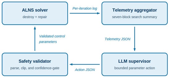
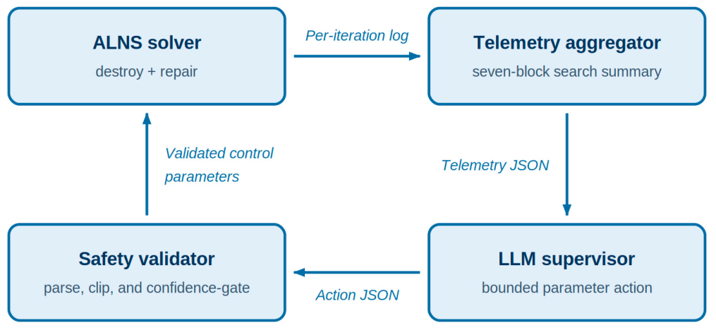
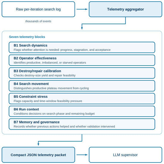
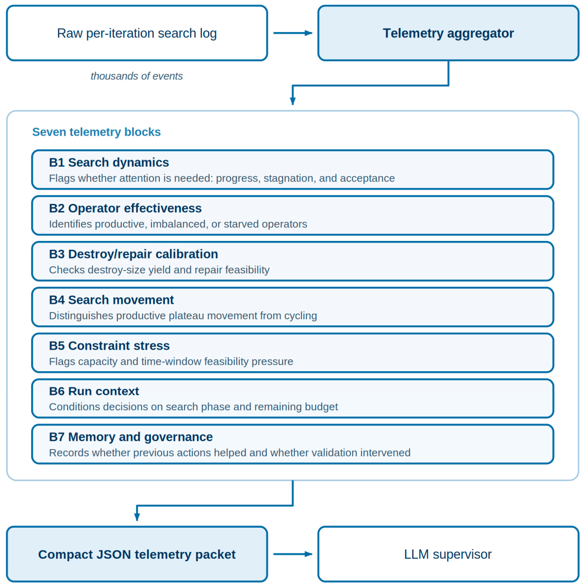
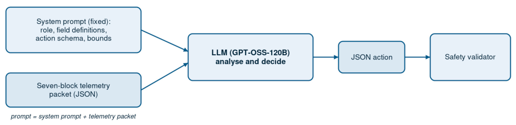
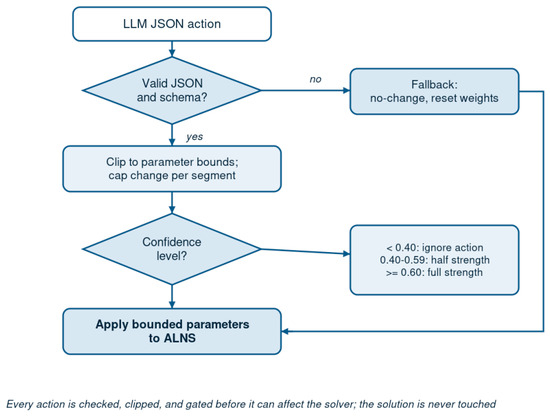
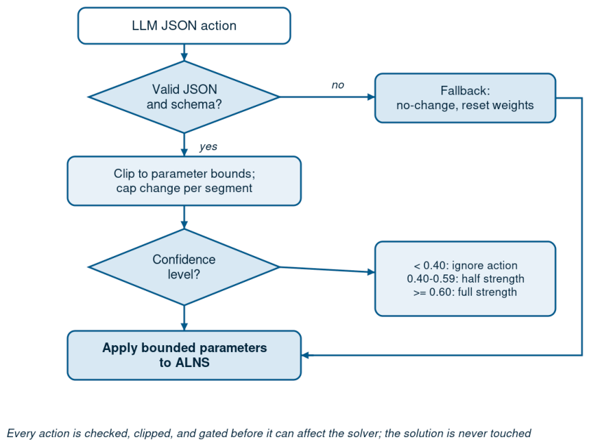
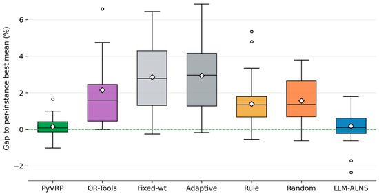
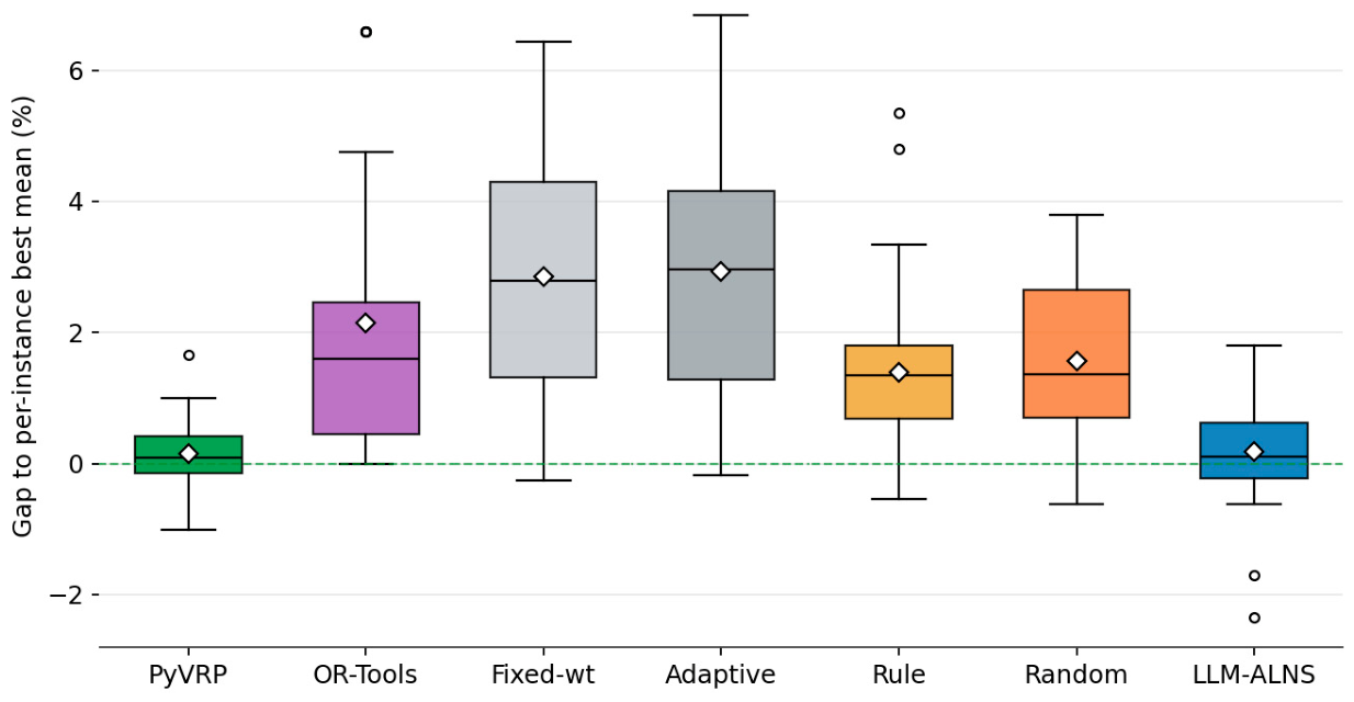
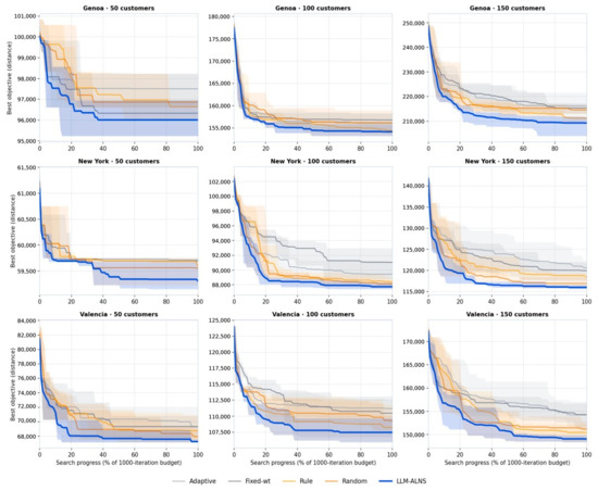
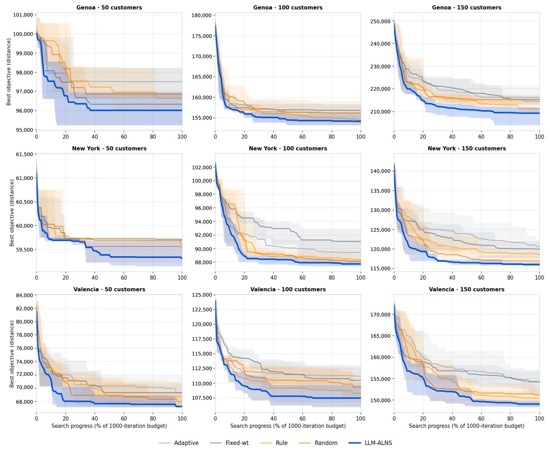
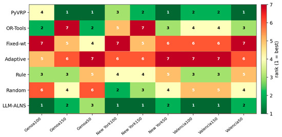
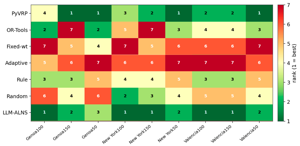
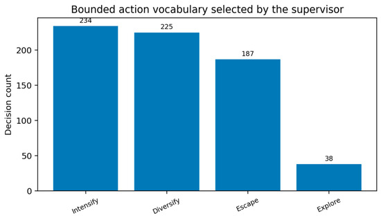
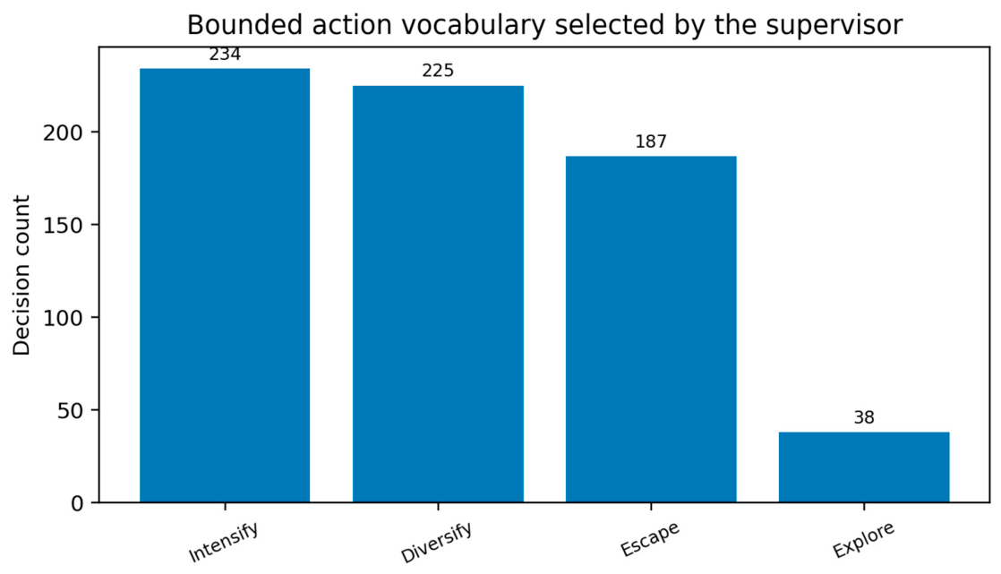
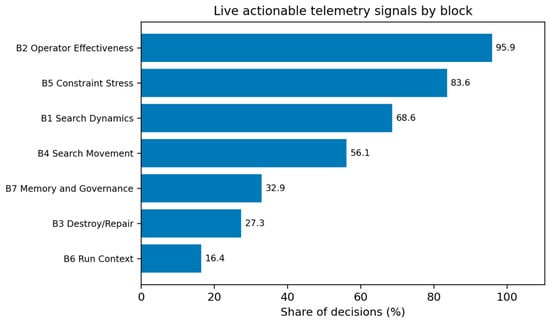

Disclaimer/Publisher’s Note: The statements, opinions and data contained in all publications are solely those of the individual author(s) and contributor(s) and not of MDPI and/or the editor(s). MDPI and/or the editor(s) disclaim responsibility for any injury to people or property resulting from any ideas, methods, instructions or products referred to in the content. |
© 2026 by the authors. Licensee MDPI, Basel, Switzerland. This article is an open access article distributed under the terms and conditions of the Creative Commons Attribution (CC BY) license.