


Abstract
The paper explores the use of artificial neural networks for surface roughness parameter Ra prediction when milling the finishing of flat surfaces with toroidal milling on C45 steel. The experiments were conducted on a 5-axis CNC center, varying three main parameters: cutting speed, feed per tooth, and tool axis tilt angle. In total, 70 surfaces were processed, with multiple measurements of Ra roughness. The data were preprocessed in MATLAB (noise reduction by Z-score and augmentation to 630 values) and used to train an artificial feedforward neural network with Bayesian regularization. The resulting model showed good performance on the dataset and was experimentally validated on three new parameter combinations, processed and measured independently with a 3D scanner. The results confirm the network’s ability to estimate Ra roughness based on varying process parameters. The paper proposes the model as a useful tool for assessing surface quality in finishing milling and recommends extending the experimental base as the main direction of continuation.
1. Introduction
In general, the functional surfaces of engineering components are designed in such a way as to meet certain quality requirements, frequently quantified by the roughness parameter Ra. This requirement has generated a sustained interest in research, oriented towards investigating and establishing rigorous correlations between the roughness value and the behavior of the cutting tool during machining.
Milling is one of the basic processes of machining technologies, being widely used in the machining industry for obtaining the geometry and finishing of metal components, as evidenced in the literature [1,2,3]. The performance of the final product is directly influenced by the quality of the surface obtained and the accuracy of the execution of the technological process, as well as its efficiency; all these factors essentially contribute to the sustainability in operation.
From the perspective of the machined material, C45 steel [4,5], due to its favorable mechanical properties and extensive use in the field of engineering, requires special attention to the cutting regime. Thus, optimizing the parameters of the milling process becomes a prerequisite for obtaining high-quality surfaces and increasing productivity [6,7]. In this context, the fundamental technological parameters—cutting speed (vc), feed per tooth (fz), and cutting depth (ap)—play a decisive role in both the surface roughness value (Ra) and the material removal rate, directly influencing the overall efficiency of the milling process [8,9].
In recent years, several works on processing processes have focused on the use of artificial neural networks to model surface roughness. Even in such a specific niche of literature, the papers differ considerably in terms of how they define network architectures and validation of results, as well as their training algorithms, error measures, and the like. Moreover, an examination of individual papers leaves a researcher without a clear view of what surface quality prediction is.
An important advantage in meeting this new challenge is to quickly obtain information on specific processing operations. When the key role in such operations is economic, knowing the optimal processing parameters is vital. Researchers who want to gather such knowledge have proposed the use of machinability models. For Paiva et al. [10], these models can be used as objective functions in optimization, simulation, control, and planning.
Studies applied to surface roughness modeling have a significant number of options available to them in terms of modeling roughness data. For various reasons, only one option has been largely investigated in the literature, and that is the use of artificial neural networks. The artificial neural network is a paradigm of artificial intelligence; this is what El-Mounayri [11] and Coit [12] argue as having the possibility of having many attractive properties for modeling complex production systems. The main feature of neural networks is that they are able to find the rule that connects the output and input parameters during the training process. When the neural network is trained, it also works in situations that it has not faced during the training process [13,14,15,16].
The neural network is a highly flexible modeling tool capable of learning the mapping between input and output parameters. An artificial neural network is capable of learning from an experimental dataset to more effectively describe nonlinear and interaction effects [16]. The network consists of an input layer used to present the data, the output layer to produce the response of the artificial neural network, and one or more layers hidden in between. The network is characterized by the topology, weight vectors, and activation function that are used in the hidden and output layers of the network [17,18].
MATLAB 2024a provides command-line functions and applications for creating, training, and simulating artificial neural networks. The applications facilitate the development of neural networks for tasks such as classification, regression (including time series regression), and clustering.
The MATLAB program has a collection of functions and graphical interfaces, intended for working with artificial neural networks, grouped under the name of Neural Network Toolbox. As a result, I decided to use the MATLAB software to create the artificial neural network. Before starting to create an artificial neural network, it is necessary to create input data and output data. This is where the computer resources debated in previous papers [19,20,21,22] come in.
In the literature, several researchers have proposed and analyzed models based on artificial intelligence, used to estimate processing times, obtaining average errors of about 10–20 min [23]. Models capable of estimating the duration of the manufacturing process with a percentage error of less than 25% have also been developed [24]. In addition, the use of artificial intelligence tools for estimating production costs since the design stage has been a topic of interest for various studies [25,26,27,28] as well as the evaluation of the effectiveness of different types of artificial neural networks (ANNs) in predicting processing times [29].
The prediction of the surface quality obtained from the milling process is a rigorous technical and economic basis for ensuring the performance of the processed surfaces. The implementation of artificial neural networks in estimating surface quality allows significant savings in time, material resources, and energy. In order to obtain predictions as close to reality as possible, the datasets used in the training process are an essential element. Few research studies investigate the milling process with 5-axis toroidal milling cutters, especially the influence of the tilt angle on the surface quality. In addition, there is a lack of predictive models experimentally validated by independent measurements on new surfaces. To address this gap, the present paper aims to carry out an experimental study on the influence of cutting speed, tooth feed, and tilt angle on the roughness Ra when milling flat surfaces with a toroidal milling machine on C45 steel; to develop a model based on artificial neural networks with advanced data preprocessing; and to validate the accuracy of predictions through independent experiments using a 3D scanner. Next, the methodology for conducting the experiments by which the input and output data of the neural network are obtained, as well as the stages of their processing, in order to develop and test a system for predicting the surface quality, expressed by the roughness parameter Ra, is presented. Taking into account the literature on the early phase of the involvement of artificial neural networks in the prediction of roughness, I consider this topic innovative and prospective in terms of what future research based on surface quality may mean.
2. Experimental Research on the Processing of Flat Surfaces with Toroidal Milling Cutters
The experimental design was carried out based on the principles of the Taguchi method. Three control factors have been defined with 7, 3, and 4 levels, respectively, for vc, fz and β. Although a standard orthogonal matrix was not used, an equilateral hybrid design was adopted that led to 70 experimental combinations, allowing the evaluation of the main effects and interactions between parameters. In the experiments to be carried out, the main factors of interest are:
- •
- Cutting speed—vc [m/min];
- •
- Feed per tooth—fz [mm/tooth];
- •
- The tilt angle—β.
The tilt angle to the surface’s normal was denoted with β, the notation β for this parameter being frequently found in the literature.
The three factors mentioned above are established in order to determine the most favorable level, to increase the performance of the milling process, and to obtain a minimum influence of uncontrollable factors and, at the same time, to obtain the best possible surface quality.
The design of the experiment was carried out on the C45 material, considering this material as a common one both in the automotive industry and not only, using only flat surfaces from a geometric point of view, each surface being roughened and semi-finished in a previous process, the research focusing only on the finishing processing with the toroidal mill.
2.1. Description of Experiments
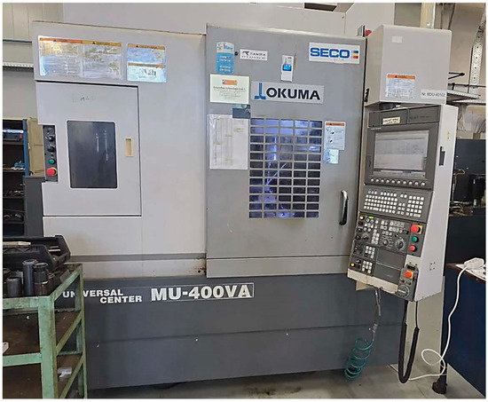
The experimental research was carried out within the company S.C. Ramira S.A., a joint-stock company, with the work point in Baia Mare, Romania being a member of the Chropynska SA group. The experiments were carried out on an OKUMA MU-400VA 5-axis numerical control center, produced in Ōguchi, Aichi Prefecture, Japan, as in Figure 1. The Okuma MU-400VA is a 5-axis vertical CNC, equipped with strokes of approx. X = 762 mm, Y = 460 mm, Z = 460 mm, and a Ø400 mm trunnion rotary table with a maximum load capacity of 300 kg and additional axes A (+20°/−110°) and C (360° continuous rotation). The main shaft has a speed of up to 15,000 rpm, a BT40 cone, a power of about 22 kW, and the tool magazine can reach 48 positions with an automatic changer.
Figure 1.
5-axis CNC machine MU-400VA.
As geometric characteristics of the specimens, they have a width of 40 mm and a length of 40 mm and a thickness of 20 mm, being made of C45 carbon steel with flat surfaces.
Before the experimental research on surface processing, the specimens are milled laterally to ensure a grip as rigid as possible; the way of gripping them will be carried out with the help of a vise with an imprint. The research is carried out only on the surface finishing processing, which means that the roughing processing in the case of all surfaces will be carried out on another CNC center.
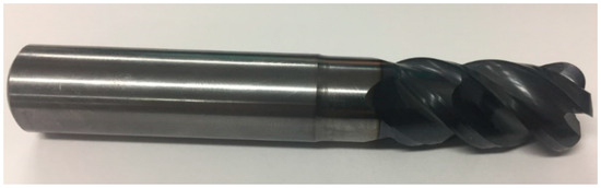
The processing of the surfaces was carried out with a toroidal milling machine with a diameter of Ø16, as in Figure 2. The JHP780160E2R400.0Z4-M64 milling cutter from Seco Tools, produced in Wholesaler in Gorinchem, The Netherlands, is a solid carbide monobloc milling cutter with a diameter of 16 mm, 4 edges, and a corner radius of 4 mm, with a cutting length of 32 mm and a total length of 100 mm with a helix angle of 44°. The tool is coated with a MEGA-64 PVD protective coating, which provides high resistance to wear and high temperatures. This tool cutter is part of the class of high-performance machining tools, being designed for intensive regimes with large cutting depths and widths. This tool provides stability and high productivity in the processing of steels, stainless steel, and difficult alloys.
Figure 2.
Toroidal milling cutter JHP780160E2R400.0Z4-M64 with a diameter of Ø16.
The selection of ranges for the cutting parameters was deliberately carried out in order to investigate a wider range than recommended by the tool manufacturer in order to fully understand the behavior of the toroidal milling process. Thus, the cutting speed was varied between 80 and 210 m/min, exceeding the manufacturer’s recommended range (140–160 m/min), in order to evaluate both the perforation at low speeds (where better roughness is usually achieved) and at higher speeds (where more pronounced thermal and dynamic effects occur). The tooth feed was chosen around the recommended value (0.15 mm/tooth), with ±27% variation (0.11 and 0.19 mm/tooth), to capture the influence of this parameter on roughness.
As regards the angle of inclination of the tool axis (β), in the absence of any reorders from the manufacturer, the values 15°, 35°, and 55° have been selected, covering a relevant range for 5-axis milling. These values allow the analysis of the effect of the angle of inclination on the tool material contact geometry and, implicitly, on the surface quality. The choice of a wide range of parameters aims to identify general trends and optimal combinations, going beyond the limits of conventional manufacturers’ recommendations. All the various parameters are summarized in Table 1.
Table 1.
Toroidal milling cutter cutting regimes.
Regarding the experimental conditions, the axial cutting depth was kept constant throughout the duration of the experiments, having the value ap = 0.5 mm, and the radial cutting depth was set at ae = 0.3 mm. The processing was carried out in the presence of the cutting fluid, with the specimens being rigidly fixed in the vise.
Also, during surface processing with the toroidal milling machine, the tool axis maintained a constant angle of inclination with respect to the processed surface.
For each specimen, the CAM programs were developed using PowerMILL 2015 software, using specific tool definition options and selection of the optimal machining strategy. Thus, for each surface analyzed, machining was carried out in a single direction, with parallel tool trajectories.
The surface roughness measurement was carried out according to the ISO 4287:2010 standard. On each processed surface, three measurements were made parallel to the feed direction using a TR-200 roughness meter. The measurement parameters (cut-off length 0.8 mm and evaluation length 4 mm) were selected according to ISO 4288:1996. To validate the results, the test surfaces were additionally analyzed with a Profilm3D optical 3D scanner according to the principles of ISO 25178-2:2012.
The experimental uncertainty of the measurements was evaluated by calculating the standard deviation for the three measurements made on each surface. The mean standard deviation of the replicas resulted in 0.114 μm and the median 0.101 μm. These values indicate a good repeatability of roughness measurements, the observed variations being attributed both to the accuracy of the TR200 roughness meter produced by TIME Group Inc., headquartered in Beijing, China, and to the local micro-inequalities of the processed surface.
2.2. Machining of Flat Surfaces with a Toroidal Milling Cutter
In the experimental study, a total of 70 surfaces were processed using toroidal milling. The cutting regimes corresponding to each processing are summarized in Table 1.
The analysis of the CAM programs showed that for the full surface processing, in the case of toroidal milling, 140 machining paths were required for a 15° tilt angle, 142 trajectories for the 35° angle, and 139 trajectories for the 55° angle.
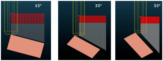
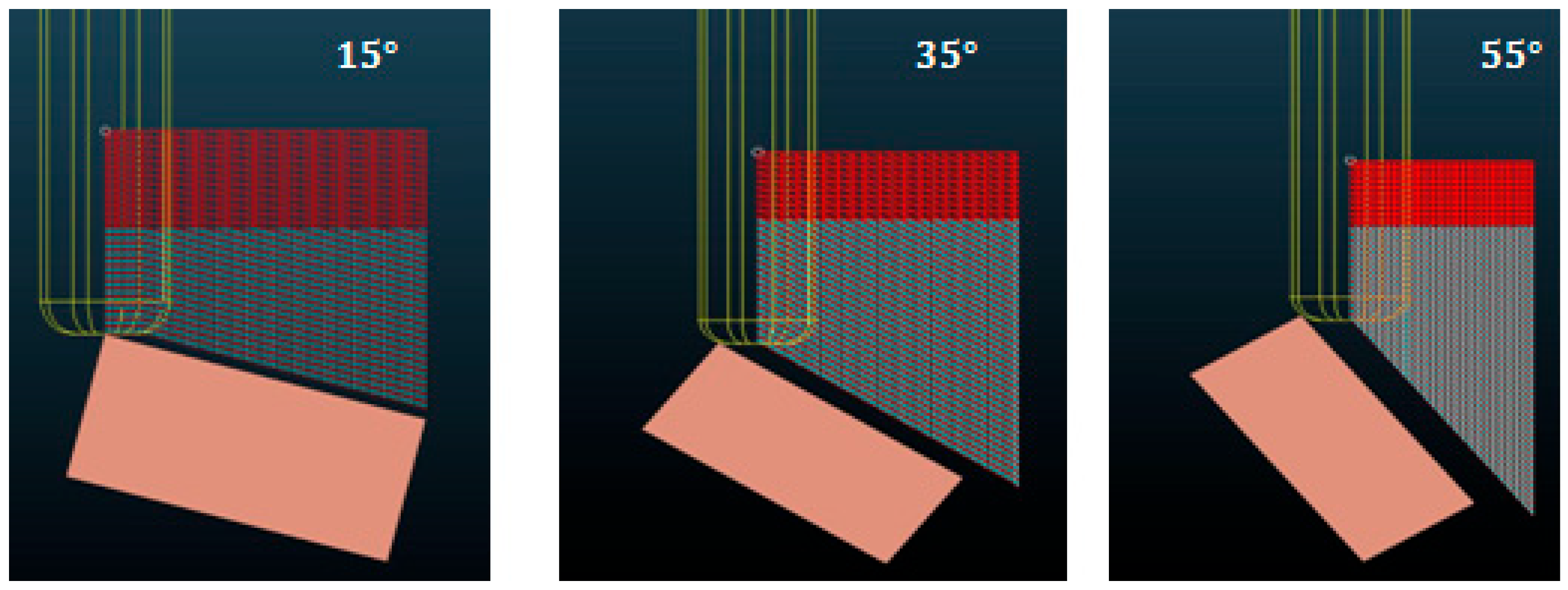
Figure 3 shows the simulations of the trajectory of the toroidal cutter during the machining of the flat surface, corresponding to the three values of the angle of inclination analyzed.
Figure 3.
CAM simulation of flat surface machining with a toroidal milling machine. (red lines-maximum feed, white lines-working feed).
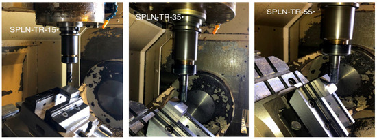
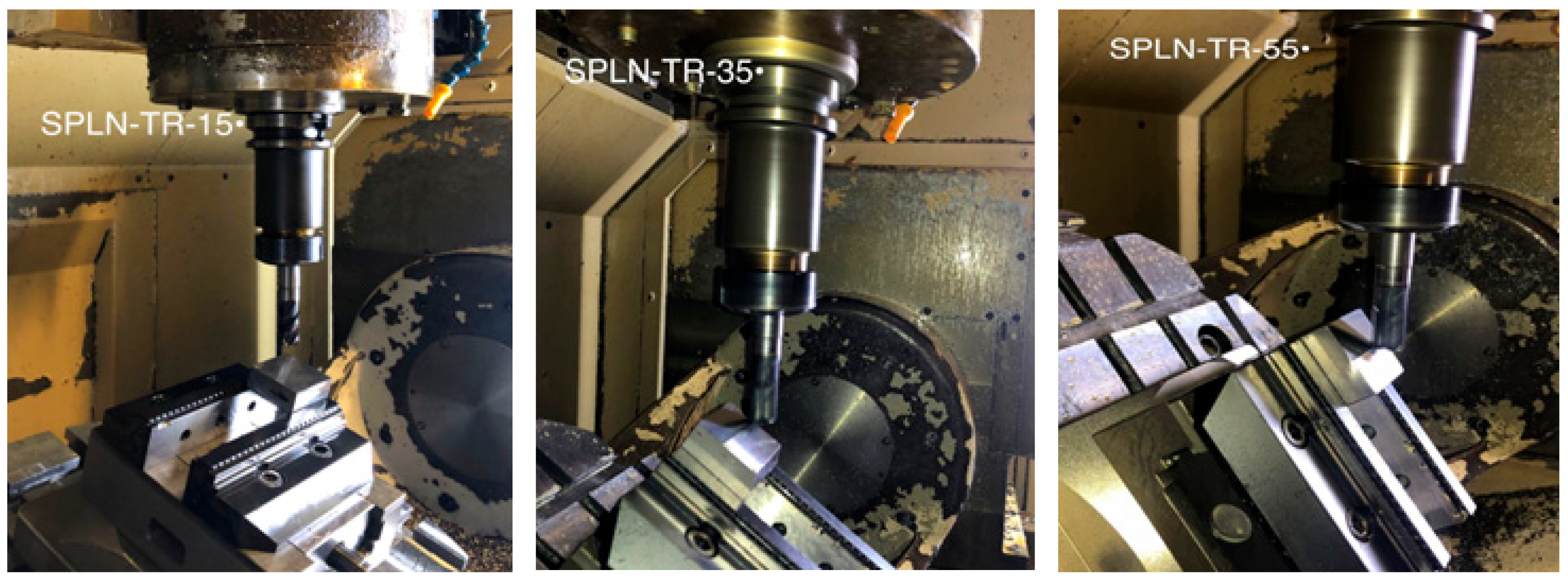
Figure 4 shows images captured during the toroidal milling process of the flat surface milling machine, carried out on the Okuma MU-400VA CNC machining center, produced in Ōguchi, Aichi Prefecture, Japan.
Figure 4.
Machining flat surfaces with a toroidal milling cutter.
2.3. Resulting Surface Quality
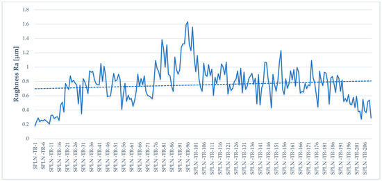
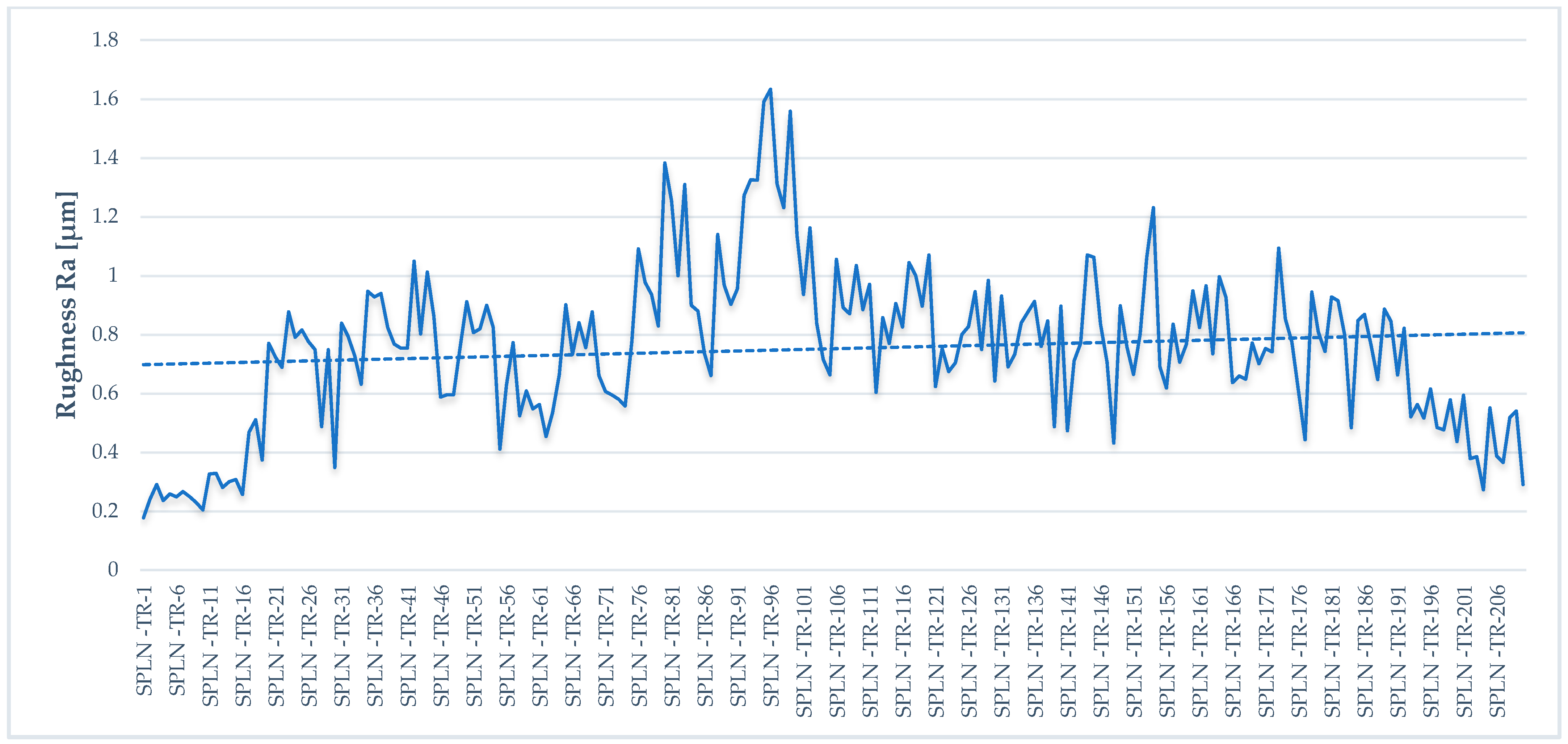
Regarding the analysis of the flat surfaces processed with the toroidal milling cutter, according to the data presented in Figure 5, the lowest value of the arithmetic average roughness, Ra = 0.177 μm, was obtained from the measurements made in the direction parallel to the feed for the flat surface processed with the toroidal milling cutter number 1 (SPLN-TR-1). The cutting regimes used in this case were cutting speed vc = 80 m/min, feed per tooth fz = 0.11 mm/tooth, and 15° tool axis inclination angle, according to Table 2.
Figure 5.
Arithmetic mean Ra of the flat surface processed with the toroidal milling cutter.
Table 2.
Experimental results related to the processing of the flat surface with the toroidal milling machine.
The highest roughness value, Ra = 1.633 μm, was recorded in measurement 3 for the SPLN-TR-32 surface, machined with the cutting regimes vc = 130 m/min, fz = 0.15 mm/tooth, and a tool axis tilt angle of 55°, according to Table 1.
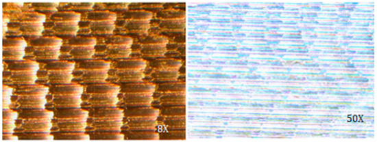
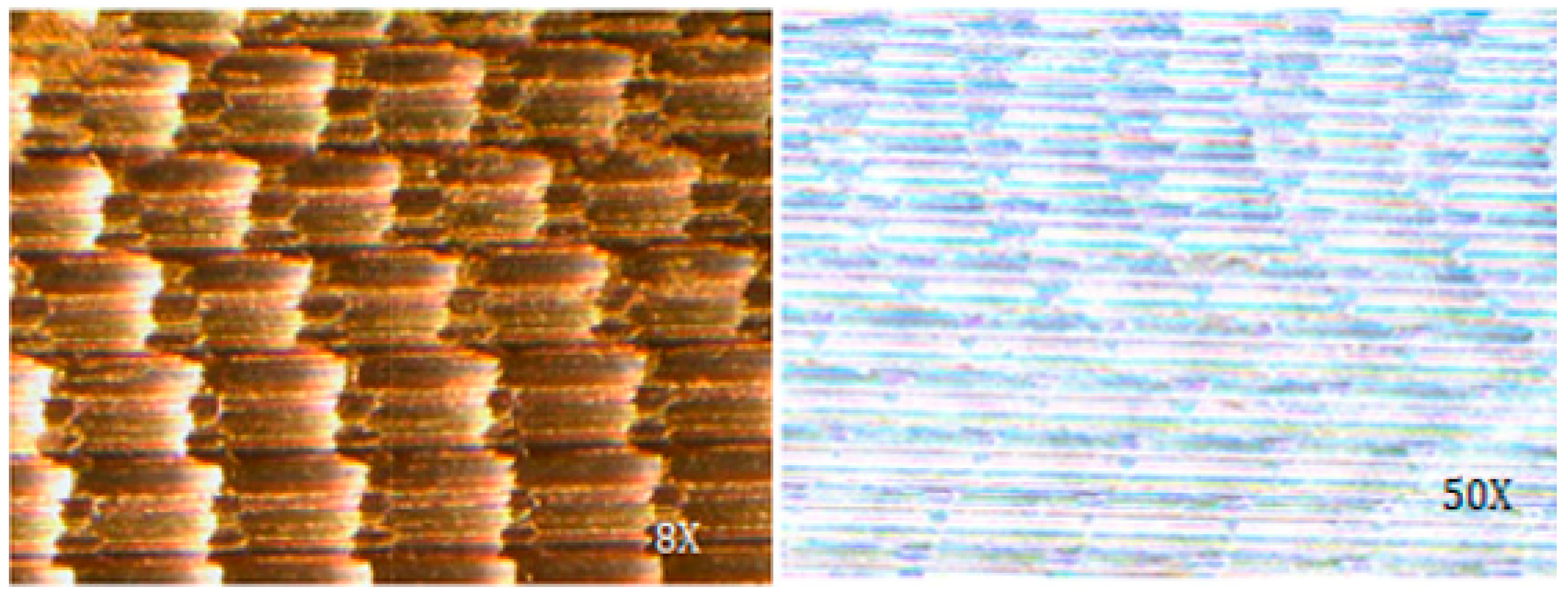
Figure 6 shows microscopic images of the best flat surface processed with the toroidal milling machine (SPLN-TR-1), obtained with the IOR stereoscopic microscope produced in Bucharest, Romania, with a magnification of 8×, and with the MM1-200 microscope produced by Hoffmann Group in Munich, Germany, with a magnification of 50.
Figure 6.
Microscopic images with the lowest roughness values focused at 8× and 50× parallel to the feed direction.
The analysis of the experimental results indicates a strong influence of the machining parameters on the surface quality. The tilt angle β proved to be the parameter with the greatest influence: the lowest roughness values were systematically obtained at β = 15°, while at β = 55° the highest Ra values were recorded (average increase of about 60%–80% compared to β = 15°).
The cutting speed vc has a nonlinear influence: the best results were achieved at low speeds (80–110 m/min), while at high speeds (190–210 m/min), the roughness increased moderately.
The feed per tooth had a directly proportional influence: the increase from 0.11 to 0.19 mm/tooth led to an average increase in Ra of about 25%–35%.
From the analysis of the 210 measurements, a significant dispersion of the Ra values for the same parameters can be observed (variations of up to 0.3 μm), which indicates the sensitivity of the process to uncontrolled factors (vibrations, tool wear, uniformity of the cutting fluid).
3. Data Analysis and Processing
MATLAB software was used to process and analyze experimental data due to its capabilities for noise filtering and data augmentation, as well as creating, training, and validating artificial neural networks. This software environment also allows the generation of accurate predictions on the performance of the machined surfaces, based on the learned models.
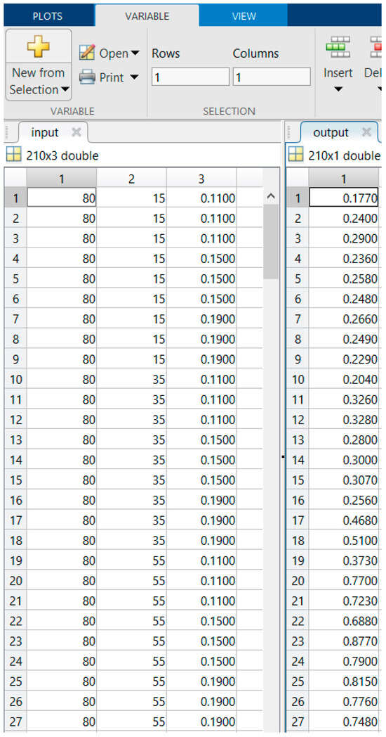
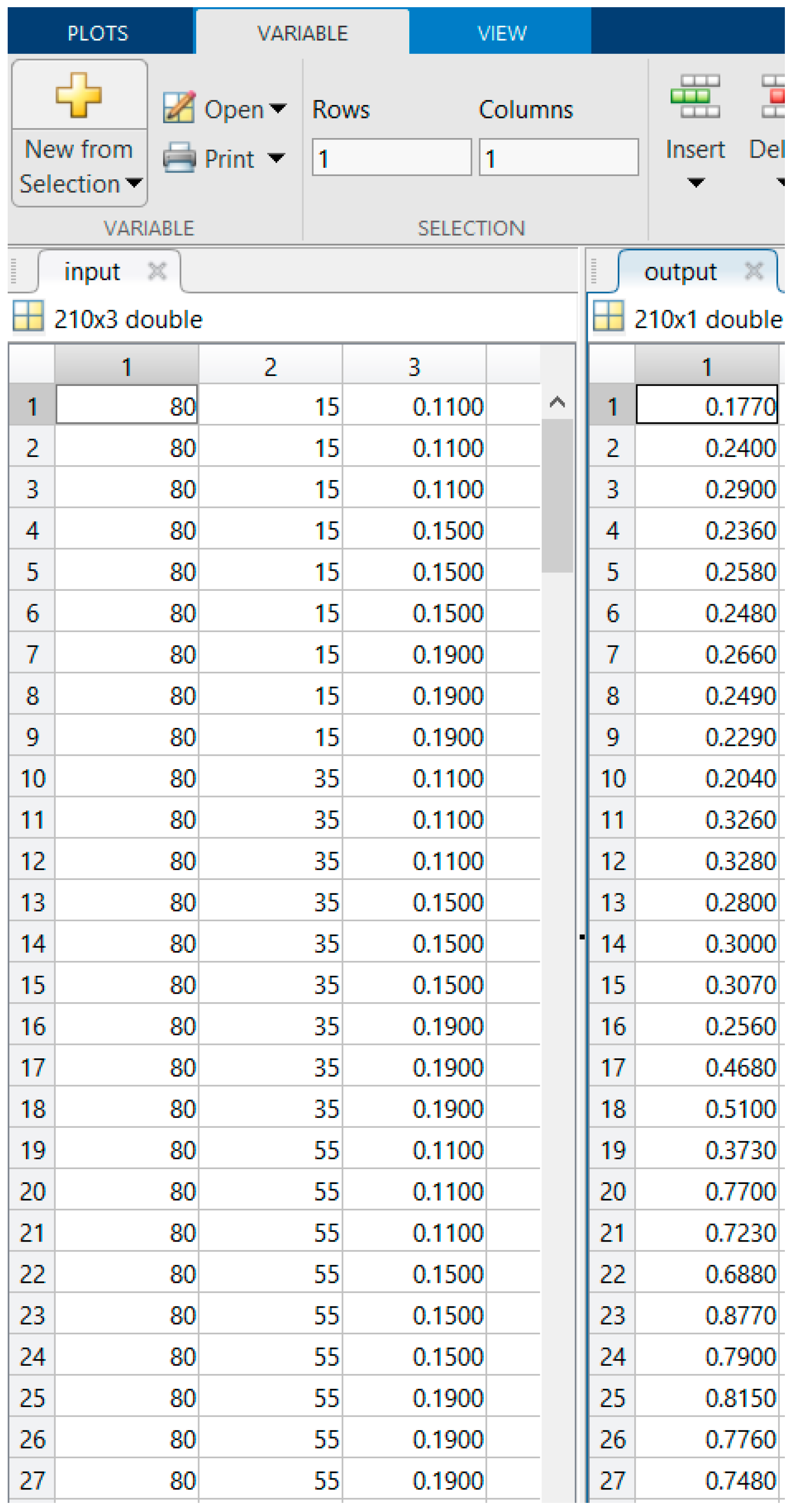
The process variables selected for the input values of the neural network (“Input”) were the cutting speed, the feed per tooth, and the tilt angle with respect to the normal of the surface, these being the parameters that directly influence the surface roughness (210 × 3). The output data, corresponding to the target values, were expressed by the surface roughness parameter Ra measured parallel to the direction of advance (210 × 1), according to the partial presentation in Figure 7.
Figure 7.
Images of neural network input and output data and data positioning in MatLab.
3.1. Noise Reduction and Outlier Replacement
In the output data preprocessing stage, the roughness values Ra n = 210 were subjected to a noise reduction by identifying and adjusting outliers, without removing any values. This procedure was carried out using the Z-score method applied to groups: for each unique combination of input parameters (vc, β, fz), the mean and standard deviation of the Ra values corresponding to that group were calculated. Subsequently, for each Ra value, the Z-score was determined, and the values for which the Z-score exceeded the threshold of 2.0 were replaced by the group average.
The choice of the Z-score threshold > 2.0 for the detection and replacement of outliers was made in accordance with standard practice in experimental data processing. According to the normal distribution, a threshold of 2.0 covers approximately 95.4% of the data, allowing only extreme values to be identified and considered outliers without removing valid data. This value represents a reasonable compromise between sensitivity and conservatism: a lower threshold (e.g., 1.5) would have led to the excessive replacement of real values, while a higher threshold (e.g., 3.0) would have left unresolved large variations caused by measurement errors.
This approach allows the entire initial dataset to be preserved while reducing the effect of extreme variations, which can be attributed to measurement errors or experimental noise. By applying this method, the data becomes more homogeneous and suitable for training the neural network, without compromising the volume of information available, the MATLAB code is shown in Figure 8.
Figure 8.
MATLAB Code and noise reduction results.
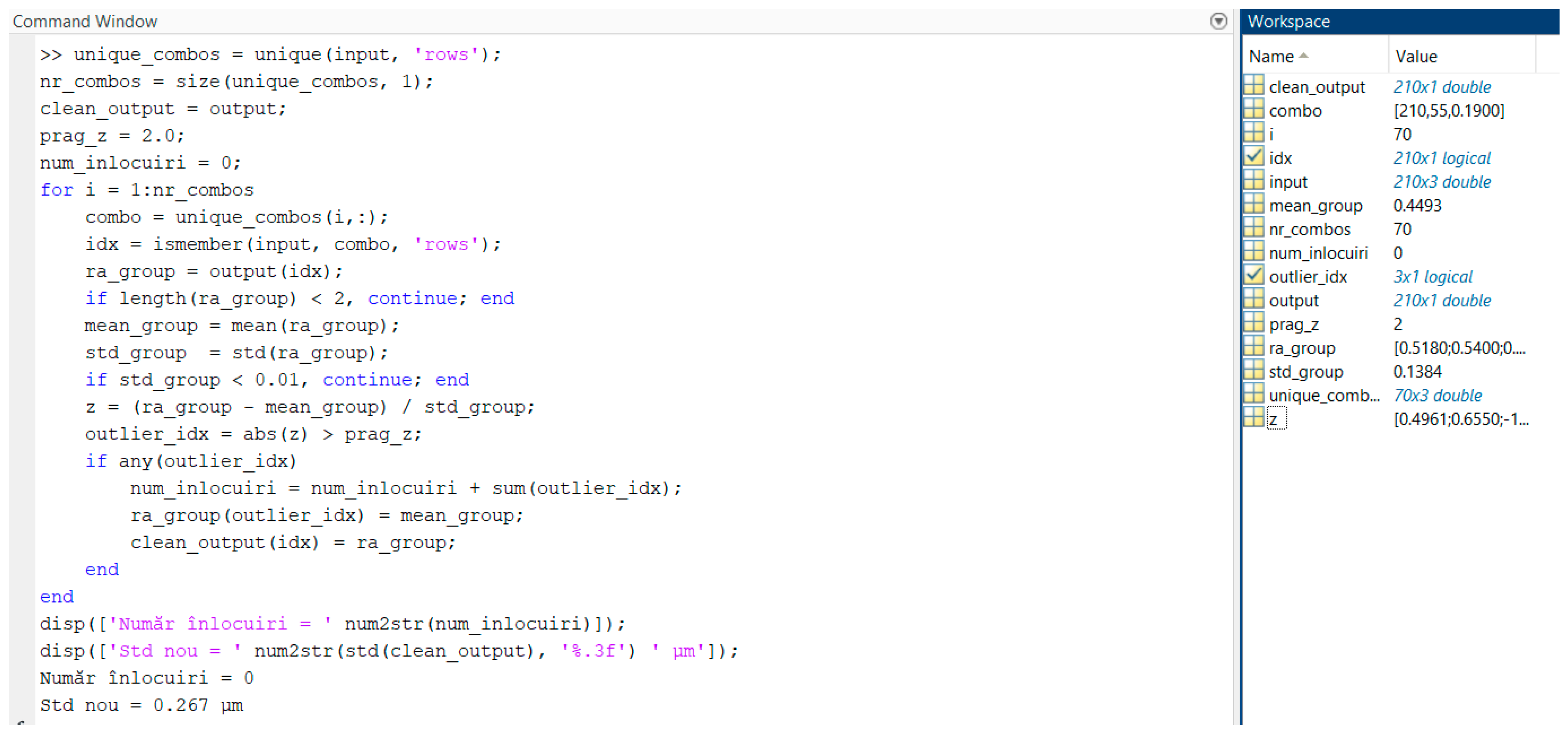
Single rows in the input array are extracted into the unique_combos to group parameter repeats, and nr_combos defines the number of them for iteration control. The vector clean_output copies the original output to preserve the original data, while prag_z sets the threshold for detecting outliers, and num_inlocuiri initializes the change counter. The for loop iterates through each combination, selected by combo, and idx identifies the corresponding positions in the input matrix, allowing the ra_group subset to be extracted from the output. Groups with fewer than two observations or with a standard deviation below 0.01 are omitted to avoid the calculation of the Z-score, which is obtained by normalizing the values against the mean (mean_group) and the standard deviation (std_group). Values with a Z-score above the threshold (outlier_idx) are identified, and num_inlocuiri is updated accordingly. Detected outliers are replaced with the group average, and changes are propagated in clean_output, while final impressions (disp) provide feedback on the number of replacements made.
Following this step, new output lists were generated, the results obtained indicating a standard deviation of 0.267, which reflects the level of dispersion of the analyzed data.
3.2. Data Augmentation
Data augmentation is an essential step in the preprocessing process, aiming to increase the diversity and volume of the data set, thus contributing to improving the robustness and generalization of the results obtained.
At this stage, the previously pre-processed dataset was augmented, increasing the number of observations from 210 to 630. This procedure was performed to increase the diversity of the set and allow for more robust neural network training without introducing significant bias. The augmentation was selectively applied to the parameters β and fz, keeping the cutting speed vc constant, and consisted of introducing a random noise with the standard deviation of 4%, simulating the real variations in the milling process. The number of replications has been set to n_aug = 2 to maintain data balance.
The data augmentation procedure was structured in several stages. In the first step, the original preprocessed values were replicated. Subsequently, for each parameter, the standard deviation was calculated, based on which selective noise was applied. In the final stage, the augmented data was integrated with the initial set, followed by checking the final size of the dataset and the resulting new standard deviation.
This approach allows for an extensive and diversified dataset while maintaining the representativeness of the original observations and contributes to the development of a robust and reliable predictive model, the MATLAB code is shown in Figure 9.
Figure 9.
MATLAB code and data augmentation results.
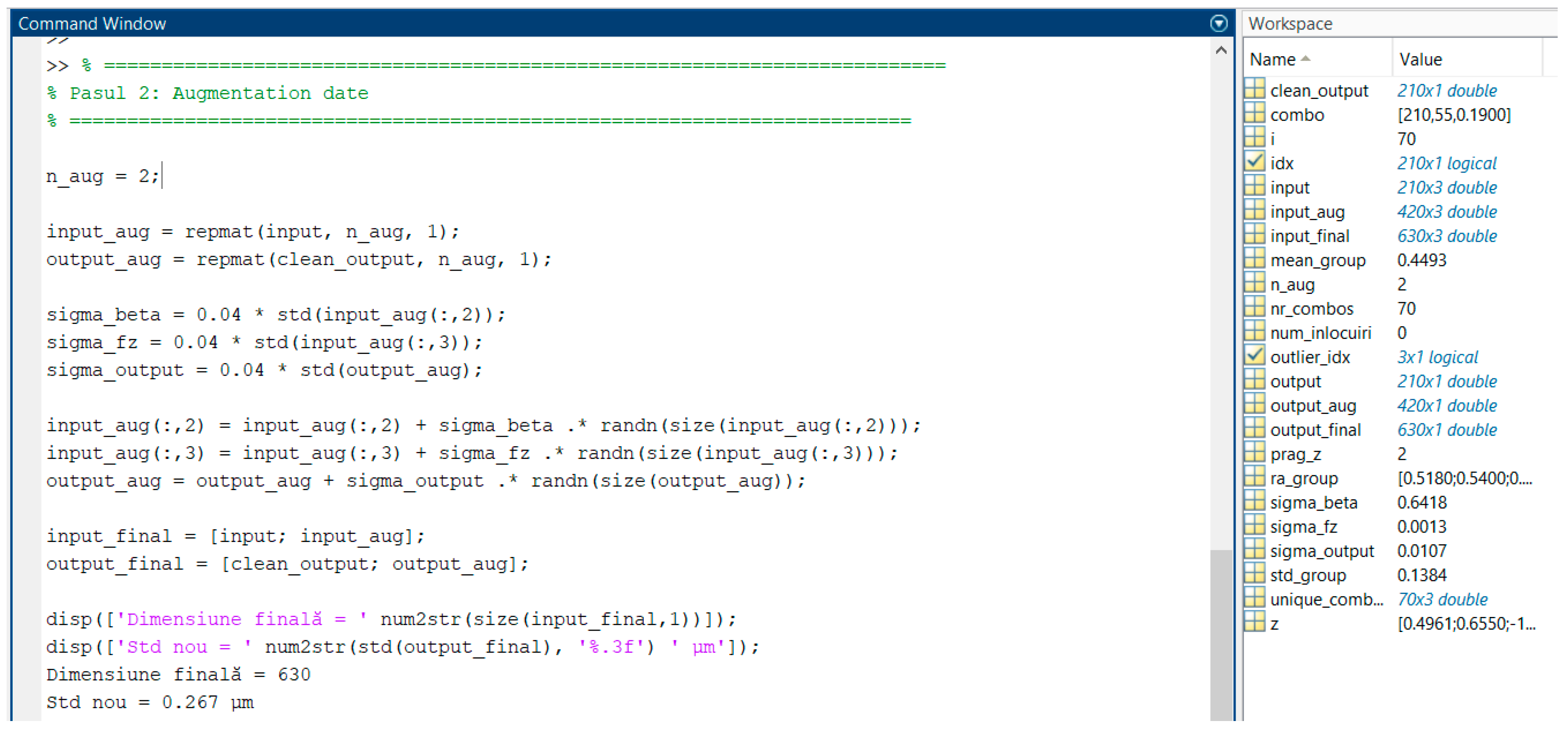
The number of new copies is set by n_aug to allow a balanced increase in the dataset, and input_aug and output_aug reproduce the input matrix and the clean output vector n_aug times, forming the basis for augmentation. The added noise is scaled by sigma_beta and sigma_fz for columns β and fz, respectively, and sigma_output for the output, corresponding to 4% of the standard deviation, to simulate realistic variations. The β and fz columns of input_aug are disturbed with normal scaled noise, and output_aug is similarly modified, introducing diversity to the augmented set. Completed input_final and output_final sets are achieved by vertically concatenating the original data with the augmented data, and the final displays (disp) provide feedback on the size and standard deviation of the extended dataset.
As a result of this step, the input_final and output_final sets were generated, corresponding to the new values obtained by augmenting the data, the final set reaching a total size of 630 values.
3.3. Artificial Neural Network ANN
To model the relationship between processing parameters and surface roughness parameter Ra, a feedforward neural network with two hidden layers was used, with 10 neurons in the first layer and 5 neurons in the second [10, 5]. This architecture has been optimized for the augmented dataset, being complex enough to capture the nonlinearities of the process but avoiding overlearning.
The training algorithm chosen was trainbr (Bayesian regularization), selected for its ability to manage the noise present in the experimental data. The dataset was divided into proportions of 70% for training, 15% for validation, and 15% for testing. Training has been carried out over 1500 eras, with a failure tolerance threshold (max_fail) of 25.
The methodological steps included the normalization of the input and output data in order to ensure a fast and stable convergence of the neural network, followed by its configuration and training according to the specified parameters. The performance of the model was then evaluated using standard statistical indicators, namely the mean absolute error (MAE), the square root of the mean error (RMSE), and the coefficient of determination (R2).
The implementation of this methodological strategy has led to the development of a robust predictive model, capable of providing accurate estimates of Ra roughness according to process parameters, while maintaining the ability to generalize the model, the MATLAB code is shown in Figure 10.
Figure 10.
MATLAB code of the ANN artificial neural network with its results.
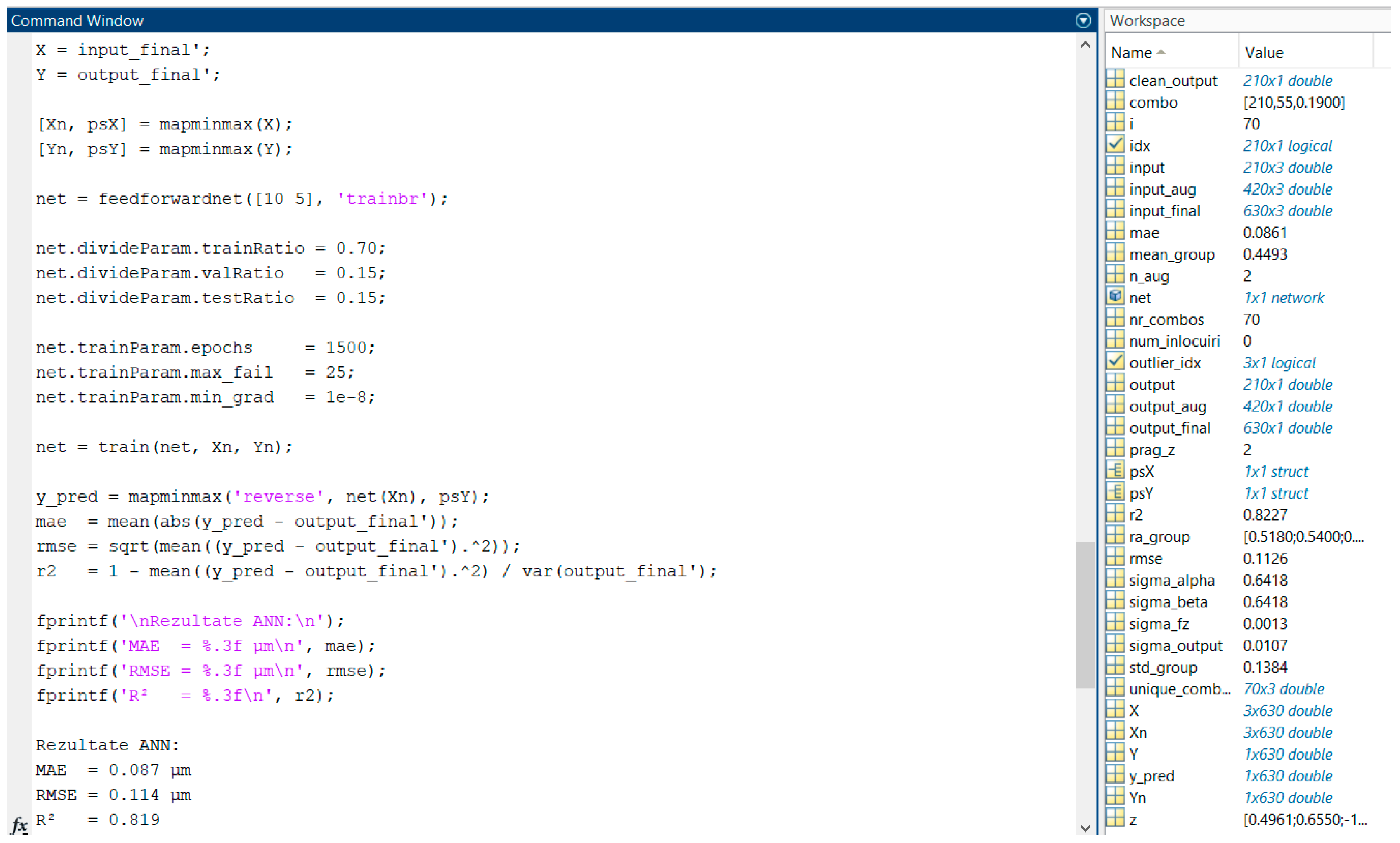
The input_final matrix and output_final vector are transposed (X and Y) to comply with the format required by artificial neural networks, and normalization is performed with mapminmax, scaling the values in the range [−1, 1] and saving the parameters for subsequent reversal (psX, psY). The neural network is defined as feedforward with two hidden layers (10 and 5 neurons) and trained by Bayesian regularization (trainbr) to handle noise and low data. The proportions for entrainment, validation, and testing are set at 70%, 15%, and 15%, respectively, and the entrainment parameters include 1500 maximum epochs, a maximum of 25 consecutive failures for early stopping, and a minimum gradient of 1 × 10⁻⁸ for ensuring convergence. Training is performed by train (net, Xn, Yn), and y_pred predictions are denormalized using mapminmax (‘reverse’). The performance of the network is evaluated by the MAE, RMSE, and the coefficient of determination R2, and the results are displayed with an accuracy of three decimal places for each metric (fprintf).
In the analysis of neural network performance, the values obtained for the statistical indicators show an absolute mean error (MAE) of 0.087, a square root of the mean error (RMSE) of 0.114, and an R2 correlation coefficient of 0.819. These results indicate a high ability to approximate the model on the dataset used for training, composed of preprocessed and augmented data.
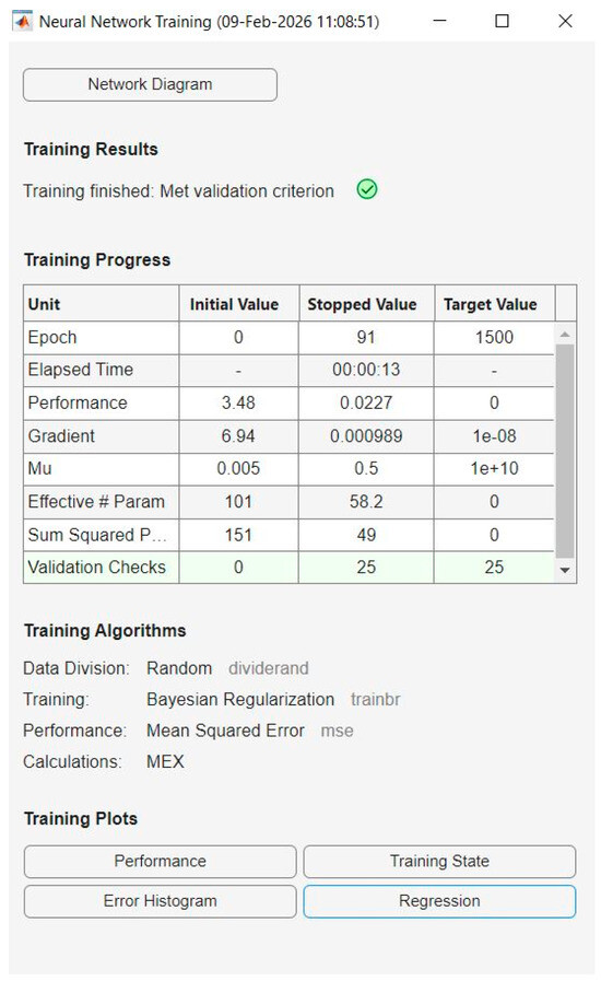
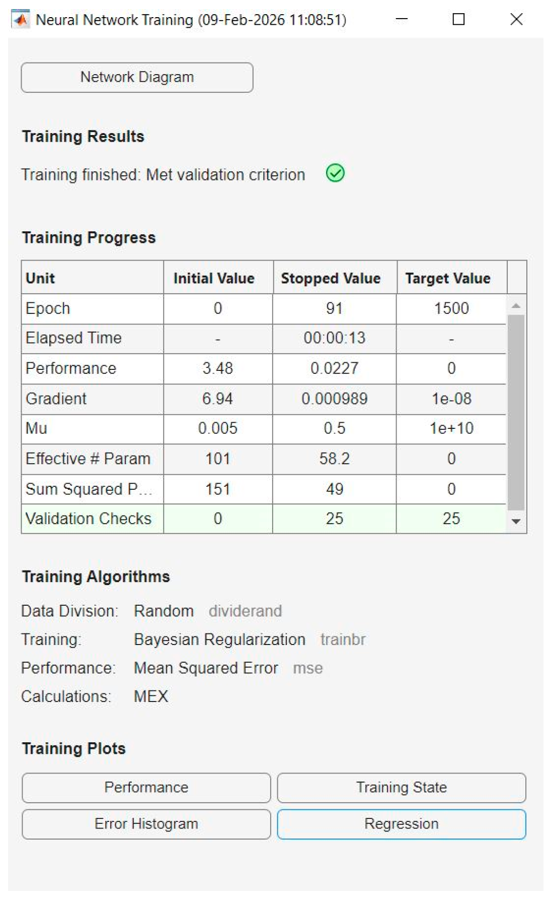
Figure 11 shows the numerical summary of the training process, indicating that the neural network has been trained for 91 epochs, the shutdown being determined by reaching the maximum threshold of checks on the validation set. The model’s performance, as measured by mean square error (MSE), saw a significant decrease from the initial value to 0.0227, highlighting an effective convergence. Low gradient values confirm stabilization of the optimization process.
Figure 11.
Neural network training.
The increase in the regularization parameter and the reduction in the actual number of parameters indicate the efficient application of Bayesian regularization, leading to a simpler and more robust model. Stopping training due to performance stagnation on the validation set suggests reaching a learning plateau, which indicates that the model has extracted the relevant information available in the current dataset. Overall, the results confirm a stable and well-controlled drive process suitable for the Ra roughness prediction application.
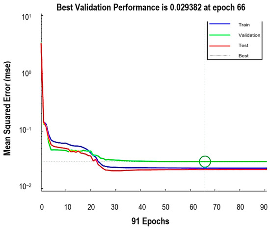
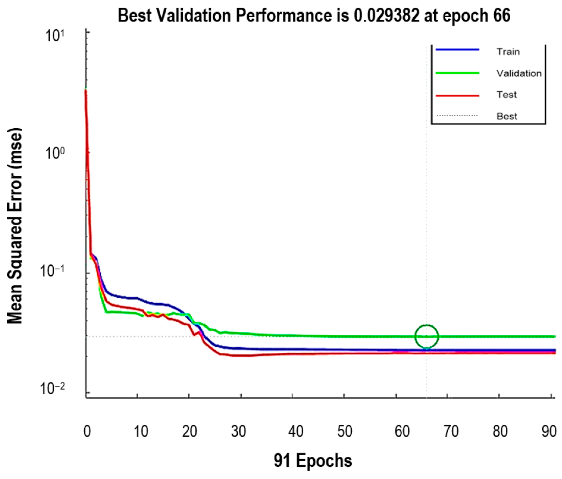
Figure 12 shows the analysis of the performance graph, highlighting the evolution of the mean square error (MSE) during the training process for the training, validation, and testing datasets. The MSE values show a progressive decrease, indicating an effective convergence of the model. Optimal performance on the validation set was reached at epoch 66, with a minimum MSE value of 0.029, after which a slight increase is observed, suggesting the onset of moderate overfitting.
Figure 12.
Performance graph (plotperform).
The proximity of the curves corresponding to the drive, validation, and test sets indicates a good generalization ability of the model, without signs of severe overfitting. The stop of training in the 91 era reflects the activation of the validation criteria. Overall, the results confirm the stable predictive performance of the neural network, with a low level of error, suitable for estimating Ra roughness.
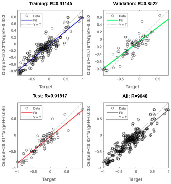
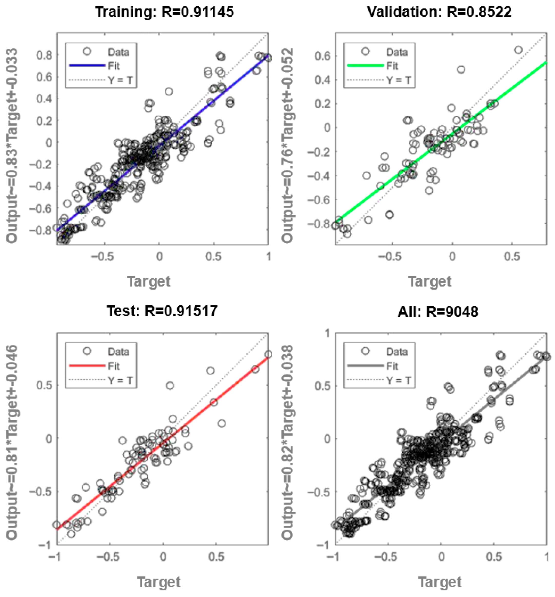
Figure 13 shows the analysis of regression plots highlighting the correlation between predicted and actual Ra values for training, validation, and test sets. The Pearson correlation coefficients (R) indicated are 0.911 for training, 0.852 for validation, 0.915 for testing, and 0.905 globally, reflecting a good ability of the model to capture linear relationships between input parameters and Ra roughness.
Figure 13.
Regression graph (plotregression).
R-values close to 1 for drive and test sets indicate a robust fit and effective generalization, while lower R-values for validation suggest the presence of residual noise or small overfitting effects. The dispersion of points around the ideal line indicates nonlinear factors or noise in the available data. Overall, the results confirm that the model shows consistent performance.
The neural model was successfully trained and demonstrated stable convergence, showing high performance on the datasets used for training (MSE ~ 0.02, global R ~ 0.90). Although the validation and test curves register slight deviations (R ~ 0.85–0.91), this indicates the presence of residual noise and not a significant overfitting, also supported by the stop of the drive as a result of the validation criteria and the efficient application of the regularization.
3.4. Prediction of Ra Values for New Combinations of Process Parameters
The prediction procedure has been simplified to eliminate iterative interactions and possible input errors. The new values of the process parameters are entered directly into an array where each row corresponds to a combination of parameters for which the roughness of Ra is to be estimated.
The algorithm runs a loop that generates the predictions for each row of the array while ensuring that the boundaries of the input range are checked and the results are explicitly displayed. This mechanism protects the model against invalid input values and provides a clear and reproducible interface for analyzing the results.
The implementation steps included defining the domain boundaries for each input parameter, creating and adjusting the matrix of new values, going through each row of it to generate predictions, and displaying the results with verification of compliance with the validity domain. This approach facilitates the rapid and reliable evaluation of process performance for new parameter combinations, reducing the need for manual intervention and preventing errors due to the introduction of invalid values, the MATLAB code is shown in Figure 14.
Figure 14.
MATLAB Ra prediction code with related results.
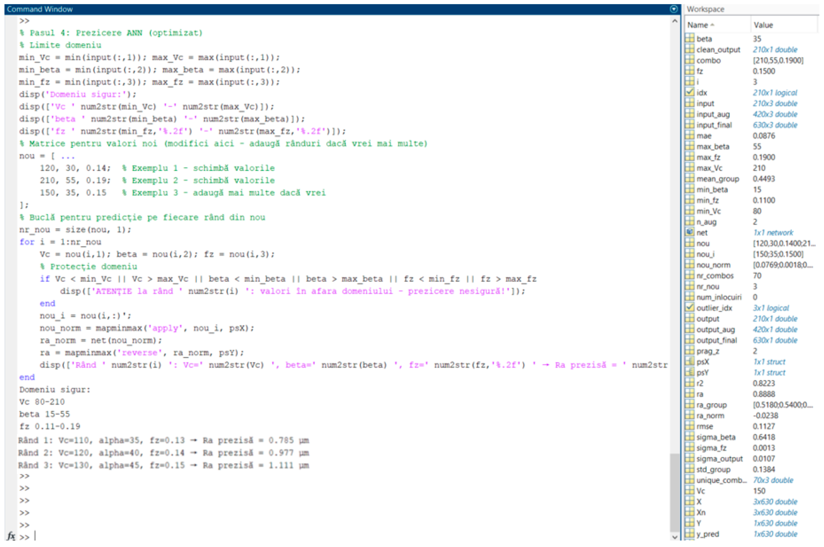
The minimum and maximum values for vc, β, and fz are calculated on the corresponding columns of the input matrix (min_vc, max_vc, min_beta, max_beta, min_fz, max_fz) to define a safe operating range, and the displays (disp) provide feedback on these ranges. The new array contains the new values for the prediction, and nr_nou determines the number of rows for the iteration. Within the for loop, the individual values vc, β, and fz are extracted from each row, and the if conditions check if they fall within the safe domain, generating appropriate warnings otherwise. The rows are transposed (nou_i) for neural network compatibility, normalized by mapminmax (‘apply’, nou_i, psX), and processed by the network for normalized prediction ra_norm, which is later denormalized (ra) to obtain the actual values. The results are displayed by concatenating the input values and the Ra (disp) prediction, providing clear feedback for each row evaluated.
Three new datasets were used to generate the predictions, which were not part of the training, validation, or testing sets. The input values were selected within the previously defined safety interval, with the aim of estimating the roughness of Ra. The three new values are shown in Table 3, and the neural network provided predictions presented in Table 3 for the roughness of Ra, demonstrating the model’s ability to extrapolate and provide consistent estimates for previously unused parameter combinations.
Table 3.
Predicting Ra roughness with new values.
4. Artificial Neural Network Certification for Predicting Ra
As presented in the previous chapter, the artificial neural network generated predictions for new values of Ra roughness based on the existing data in the database. In order to validate and confirm the accuracy of the prediction model, experimental processing of three flat surfaces was performed using a toroidal milling cutter.
The programming of the CAM process was carried out through PowerMill software, similar to the procedures used to build the initial database. The main cutting parameters were kept constant: axial cutting depth ap = 0.5 mm and radial depth ae = 0.3 mm. The machining was carried out on the OKUMA MU-400VA CNC machining center, and the clamping of the specimens was carried out in a vise with an imprint, ensuring additional rigidity and safety. The process was carried out in the presence of coolant, using the same cutting tool, a toroidal cutter with a diameter of Ø16 mm and a radius at the corner of 4 mm.
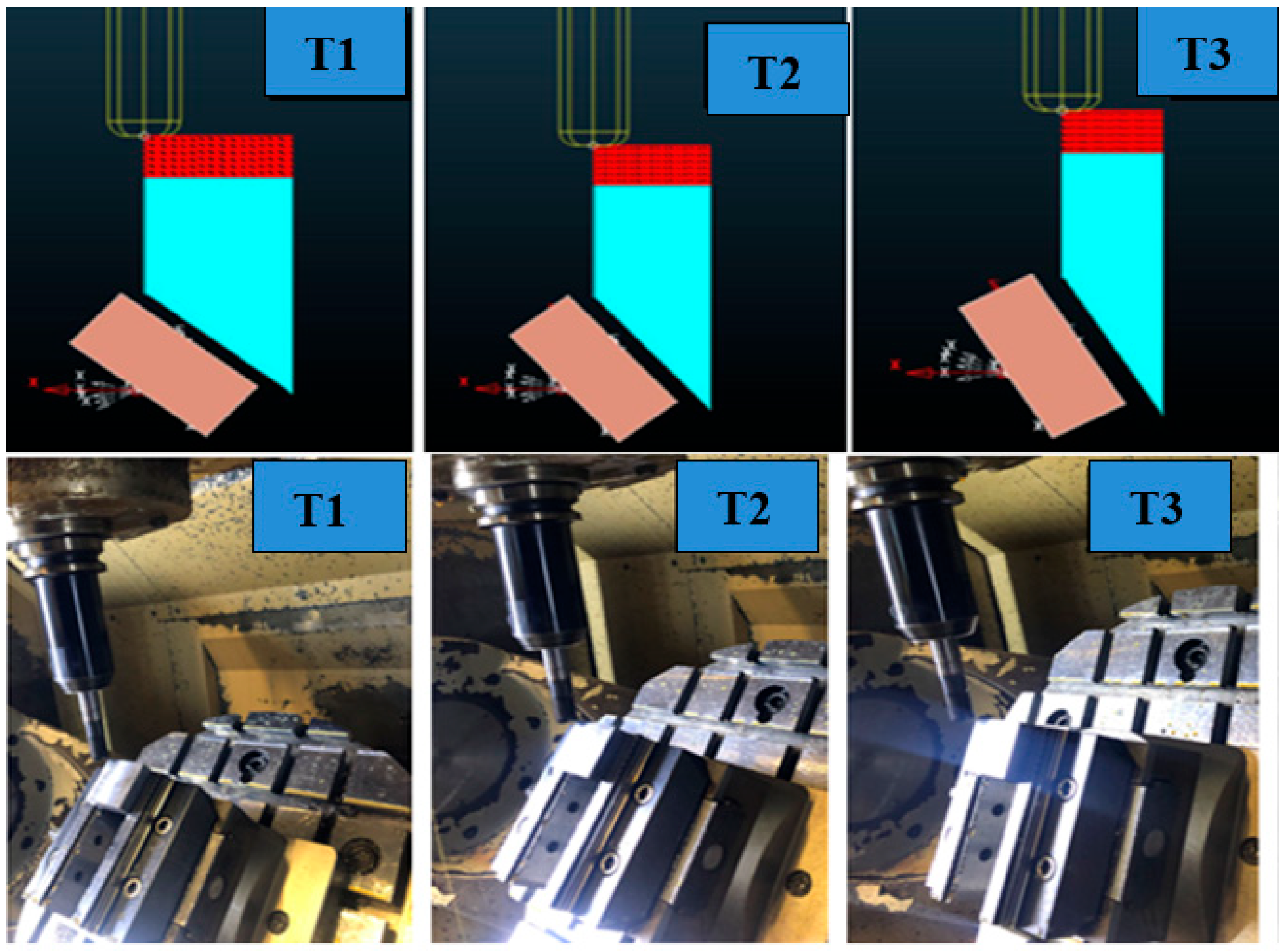
Figure 15 shows representative frames from both the process simulation in the PowerMill and the actual machining of the flat surfaces on the Okuma MU-400VA CNC center, carried out in the three experimental configurations.
Figure 15.
Images during machining and simulation of flat test surfaces with a toroidal milling cutter. (T1-T3 represents the test number).
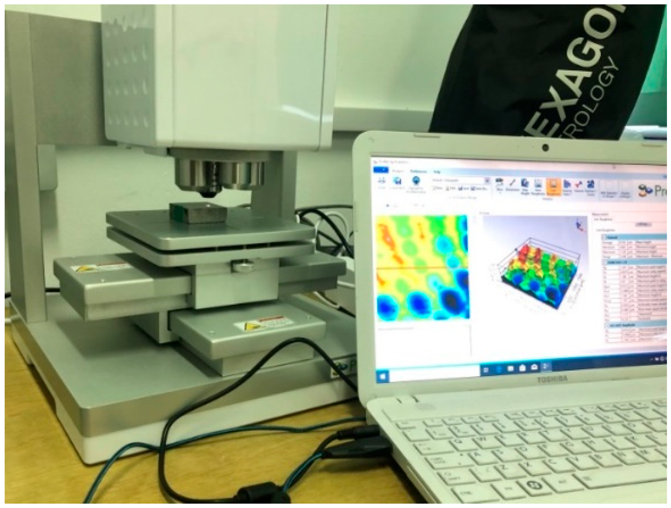
After completing the processing of the three surfaces on the CNC center, the quality of the surfaces was evaluated using a 3D scanner available at the North University Center in Baia Mare, Faculty of Engineering, shown in Figure 16. The Profilm3D system is an optical scanner that uses phase-change interferometry, providing high-precision measurements. This technology allows the analysis of surface topography on a wide range of sizes, from sub-nanometers to millimeter scale.
Figure 16.
Images during measurement of test surfaces.
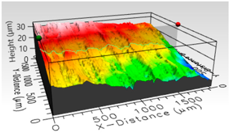
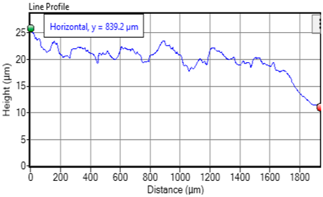
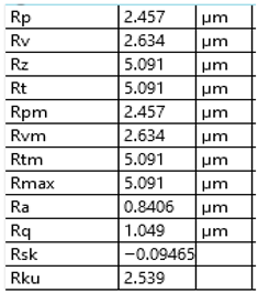
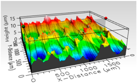
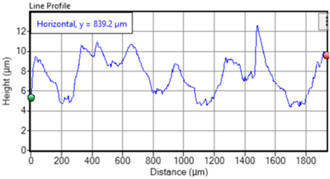
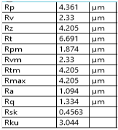
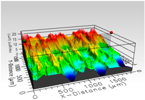
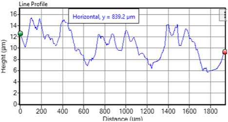
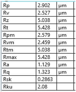
For the validation of the correctness of the measurements, the values of the roughness of the experimental surfaces are presented in Table 4. The table includes images of the 3D scanned surfaces, graphs of the measured roughness, and the numerical values corresponding to each surface, providing complete documentation of the quality of the processed surfaces.
Table 4.
Roughness parameters.
After measuring the roughness of the surfaces, the experimental values were compared with the predictions generated by the neural network. Table 5 presents these data, highlighting both actual and forecasted values, to allow the assessment of the accuracy of the model.
Table 5.
Comparable roughness values Ra.
The comparative analysis presented in Table 5 indicates an average accuracy of neural network predictions of 93.71%, with an average difference between the actual and predicted values of 0.063 μm. These results demonstrate that the model can be successfully used to estimate the roughness of Ra. However, the accuracy of the predictions depends significantly on the quality and comprehensiveness of the database used for training, and it is essential that it be as complete and accurate as possible.
5. Discussion
The experimental results reveal a significant influence of the three parameters on the surface roughness, each acting through distinct physico-mechanical mechanisms. The tilt angle (β) exerted the strongest influence. At low values (β = 15°), the contact area between the toroidal cutter and the material is reduced, and the effective cutting edge becomes sharper, which favors the formation of thin chips and a higher surface quality (minimum Ra = 0.177 μm). As β increases towards 55°, the contact area increases considerably, and the cutting geometry approaches a rounded-edge milling, generating a greater chip thickness and additional vibration. These effects lead to a marked increase in roughness (up to 1.633 μm), explaining why the angle of inclination is the dominant parameter in toroidal milling cutters.
The feed per tooth (fz) showed a directly proportional influence, according to the classical mechanism of chip formation. The increase from 0.11 to 0.19 mm/tooth increases the distance between the successive trajectories of the teeth, resulting in more pronounced notches on the surface and, implicitly, higher Ra values. The cutting speed (vc) showed a nonlinear influence. At low speeds (80–110 m/min), the roughness was smaller, probably due to a more stable chip formation and a lower temperature in the cutting area, which minimizes the phenomenon of built-up edge. At higher speeds (over 170 m/min), although productivity increases, thermal and dynamic effects (local thermal expansion and resonance-induced vibrations) occur that contribute to the slight deterioration of surface quality. The interaction between the parameters is obvious: the best results were obtained for the combination of low values (low vc, low fz and low β), while the combinations with high β led to the accentuated degradation of the roughness regardless of the other parameters. These observations confirm that optimizing surface quality in toroidal milling requires a multivariable approach, in which the tilt angle plays a decisive role.
The trained artificial neural network demonstrated stable and controlled convergence. The mean square error (MSE) decreased significantly in the first 30–40 epochs, reaching the minimum value on the validation set at epoch 66 (MSE ≈ 0.029). Training stopped at epoch 91 as a result of criterion max_fail = 25, which indicates that performance on validation data has not improved significantly in the last consecutive checks. The application of Bayesian regularization (trainbr) was effective, reducing the number of effective parameters from 101 to 58 and contributing to a simpler model less prone to severe overfitting. The values of the R correlation coefficient were very good on the training (0.911) and test (0.915) sets, with an overall value of 0.905. A slightly lower R (0.852) was recorded on the validation set, which suggests the presence of some residual noise or variations not fully explained by the three input parameters (cutting speed vc, feed per tooth fz, and tilt angle β). This modest difference between sets is considered acceptable given the experimental nature of the data and the inevitable variations in measurement.
The generated predictions for the three new parameter combinations were then experimentally validated by processing and measurement with the Profilm3D 3D scanner. The absolute error between the actual and predicted values was 0.055 μm, 0.117 μm, and 0.018 μm, respectively, resulting in an average accuracy of 93.71% and an average error of 0.063 μm. These results confirm the model’s ability to reasonably generalize to combinations of parameters that were not included in the drive set.
The performance indicators obtained on the augmented set (MAE = 0.087 μm, RMSE = 0.114 μm, R2 = 0.819) show that the network satisfactorily captures the relationship between the process parameters and the Ra roughness. However, the final accuracy remains dependent on the quality of the data preprocessing (noise reduction by the Z-score method and the Gaussian noise augmentation of 4%) and on the representativeness of the experimentally investigated intervals. The approach adopted is justified by the preliminary stage of the prediction model, implemented in MatLab, which required simplifying the analysis to a limited set of variables. In this context, the emphasis was placed on the roughness of Ra as the main indicator of surface quality, with the prospect of extending the model in future works by integrating additional variables.
For further improvement of the model, the following directions can be considered: increasing the max_fail threshold to allow driving on a slightly larger number of eras, performing several runs with different initializations and selecting the best model, expanding the database with new combinations of values of the parameters vc, fz and β, as well as introducing new variables such as cutting force, processing time, vibrations, and noise level, but also the analysis of Rt roughness, especially in the poorly represented areas of the current set.
6. Conclusions
The present paper demonstrated the successful applicability of artificial neural networks in the prediction of arithmetic mean roughness Ra for flat surfaces processed by toroidal milling on C45 carbon steel.
Experimentally, the 70 machined surfaces showed a significant variation in Ra roughness, ranging from 0.177 μm to 1.633 μm. The best surface quality (Ra = 0.177 μm) was obtained at the combination of parameters vc = 80 m/min, fz = 0.11 mm/tooth, and β = 15°. The analysis showed that the tilt angle exerts the greatest influence on roughness, followed by the feed per tooth.
Based on the experiments carried out on 70 surfaces and the subsequent processing of the data (noise reduction by the Z-score method and augmentation to 630 observations), a feedforward neural network with the architecture [10 5] was developed and trained, using the trainbr training algorithm with Bayesian regularization. The resulting model obtained good performances: absolute mean error MAE = 0.087 μm, square root of mean error RMSE = 0.114 μm, and coefficient of determination R2 = 0.819.
Independent validation on three new combinations of parameters, experimentally processed and measured with the 3D scanner, confirmed an average prediction accuracy of 93.71%, with an absolute mean error of 0.063 μm compared to the actual values obtained experimentally.
These results show that the neural network can estimate surface roughness with acceptable accuracy as a function of cutting speed, feed per tooth, and tool axis tilt angle, thus providing a useful tool for estimating surface quality in finishing milling processes.
As future research directions, the expansion of the experimental set with additional parameter values is outlined, especially in the less covered ranges, as well as the realization of additional validations on a greater number of new combinations to strengthen the robustness and scope of the model.
Author Contributions
Conceptualization, C.F.; methodology, A.O.; software, A.O.; validation, M.B. and A.O.; formal analysis, A.O. and C.F.; data curation, A.O.; writing—original draft preparation, A.O.; writing—review and editing, M.B. and C.F.; visualization, M.B.; supervision, M.B. All authors have read and agreed to the published version of the manuscript.
Funding
This research received no external funding.
Institutional Review Board Statement
Not applicable.
Informed Consent Statement
Not applicable.
Data Availability Statement
All data supporting the findings of this study are included within the article.
Acknowledgments
During the preparation of this manuscript, the authors used QuillBot Online for English language corrections (especially grammar). After using this tool/service, the authors reviewed and edited the content as needed and take full responsibility for the content of the publication.
Conflicts of Interest
The authors declare no conflicts of interest.
Abbreviations
The following abbreviations are used in this manuscript:
| ANN | Artificial Neural Network |
| SPLN-TR-(1–70) | Flat surface machined with toroidal cutter number 1–70 |
| CAM | Computer-Aided Manufacturing |
| CNC | Computer Numerical Control |
| Ra | Arithmetic Average Roughness |
| ap | Axial Depth of Cut |
| ae | Radial Depth of Cut |
| MATLAB | Matrix Laboratory (software for numerical computing) |
| MAE | Absolute average error |
| RMSE | Square root of mean error |
| R2 | Coefficient of determination |
References
- Altintas, Y. Manufacturing Automation: Metal Cutting Mechanics, Machine Tool Vibrations, and CNC Design; Cambridge University: New York, NY, USA, 2007. [Google Scholar]
- Do, T.V.; Le, N.A. Optimization of Surface Roughness and Cutting Force in MQL Hard-Milling of AISI H13 Steel. In International Conference on Engineering Research and Applications; Springer International Publishing: Cham, Switzerland, 2019; pp. 448–454. [Google Scholar]
- Rao, R.V. Advanced Modeling and Optimization of Manufacturing Processes: International Research and Development; Springer: New York, NY, USA, 2011. [Google Scholar]
- Duong, N.T.; Hung, P.V.; Canh, N.V.; Sinh, N.T. Study on anisotropy of surface friction of steel C45 conducted by fine-grinding method. J. Sci. Technol.—Tech. Univ. 2019, 29, 46–50. [Google Scholar]
- Magri, M.L.; Diniz, A.E.; Button, S.T. Influence of surface topography on the wear of hot forging dies. Int. J. Adv. Manuf. Technol. 2012, 65, 459–471. [Google Scholar] [CrossRef] [Scilit]
- Silva, F.J.G.; Martinho, R.P.; Magalhães, L.L.; Fernandes, F.; Sales-Contini, R.C.M.; Durão, L.M.; Casais, R.C.B.; Sousa, V.F.C. A Comparative Study of Different Milling Strategies on Productivity, Tool Wear, Surface Roughness, and Vibration. J. Manuf. Mater. Process. 2024, 8, 115. [Google Scholar] [CrossRef] [Scilit]
- Le, T.H.; Pham, V.B.; Hoang, T.D. Surface Finish Comparison of Dry and Coolant Fluid High-Speed Milling of JIS SDK61 Mould Steel. Eng. Technol. Appl. Sci. Res. 2022, 12, 8023–8028. [Google Scholar] [CrossRef] [Scilit]
- Urbikain, G.; López de Lacalle, L.N. Modelling of surface roughness in inclined milling operations with circle-segment end mills. Simul. Model. Pract. Theory 2018, 84, 161–176. [Google Scholar] [CrossRef] [Scilit]
- Weinert, K.; Inasaki, I.; Sutherland, J.W.; Wakabayashi, T. Dry Machining and Minimum Quantity Lubrication. CIRP Ann. 2004, 53, 511–537. [Google Scholar] [CrossRef] [Scilit]
- Paiva, A.P.; Ferreira, E.J.; Balestrassi, J.R.; Costa, P.P.; Paiva, S.C. A multivariate mean square error optimization of AISI 52100 hardened steel turning. Int. J. Adv. Manuf. Technol. 2009, 43, 631–643. [Google Scholar] [CrossRef] [Scilit]
- Kishawy, H.; Briceno, H.; El-Mounayri, J. Otimization of CNC ball end milling: A neural network-based model. J. Mater. Process. Technol. 2005, 166, 50–62. [Google Scholar]
- Jackson, D.W.; Smith, B.T.; Coit, A.E. Static neural network process models: Considerations and case studies. Int. J. Prod. Res. 1998, 36, 2953–2967. [Google Scholar] [CrossRef] [Scilit]
- Balic, S.; Cus, J.; Klancnik, F. Intelligent prediction of milling strategy using neural networks. Control Cybern. 2010, 39, 9–22. [Google Scholar]
- Jurkovic, G.; Cukor, Z. Optimization of turning using evolutionary algorithms. Tech. Gaz. 2010, 30, 1–10. [Google Scholar]
- Podulka, P.; Kulisz, M.; Antosz, K. Evaluation of High-Frequency Measurement Errors from Turned Surface Topography Data Using Machine Learning Methods. Materials 2024, 17, 1456. [Google Scholar] [CrossRef] [Scilit]
- Trzepieciński, T. The Comparison of the Multi-Layer Artificial Neural Network Training Methods in Terms of the Predictive Quality of the Coefficient of Friction of 1.0338 (DC04) Steel Sheet. Materials 2024, 17, 908. [Google Scholar] [CrossRef] [Scilit]
- Najm, S.M.; Paniti, I.; Trzepieciński, T.; Nama, S.A.; Viharos, Z.J.; Jacso, A. Parametric effects of single point incremental forming on hardness of AA1100 aluminium alloy sheets. Materials 2021, 14, 7263. [Google Scholar] [CrossRef] [Scilit]
- Sirants, R.; Jansons, E.; Lungevics, J. Quantitative Assessment of Micro-Vickers Measurement Precision in Relation to Surface Roughness. Coatings 2026, 16, 62. [Google Scholar] [CrossRef] [Scilit]
- Mohammad, Z.J.; Bakr, D.K. Evaluation of Fracture Toughness and Surface Roughness of a Novel Experimental Short Fiber-Reinforced CAD/CAM Block Material (In Vitro Study). Coatings 2025, 15, 1485. [Google Scholar] [CrossRef] [Scilit]
- Hong, M.; Buck, D.; Yuan, Z.; Xu, C.; Zhu, Z. Multi-Factor Analysis of Cutting Parameters for Bamboo Milling. Coatings 2025, 15, 1148. [Google Scholar] [CrossRef] [Scilit]
- Gao, Z.; Liu, S.; Zhu, L.; Li, C.; Cao, Y.; Shi, G. Composition Optimization of Coating Machine Oven Manufacturing Services Based on Improved Sparrow Search Algorithm. Coatings 2025, 15, 636. [Google Scholar] [CrossRef] [Scilit]
- Maurya, A.K.; Tiwari, S.; Bhavani, A.G.; Park, N.; Reddy, N.G.S. Artificial Neural Network-Based Modeling of Atmospheric Zinc Corrosion Rates Using Meteorological and Pollutant Data. Coatings 2025, 15, 538. [Google Scholar] [CrossRef] [Scilit]
- Atia, M.R.; Khalil, J.; Mokhtar, M. A Cost estimation model for machining operations; an ann parametric approach. J. Al-Azhar Univ. Eng. Sect. 2017, 12, 878–885. [Google Scholar] [CrossRef] [Scilit]
- Florjanič, B.; Kuzman, K. Estimation of time for manufacturing of injection moulds using artificial neural networks-based model. Polim. Čas. Plast. Gumu 2012, 33, 12–21. [Google Scholar]
- Yoo, S.; Kang, N. Explainable artificial intelligence for manufacturing cost estimation and machining feature visualization. Expert Syst. Appl. 2021, 183, 115430. [Google Scholar] [CrossRef] [Scilit]
- Djurović, S.; Lazarević, D.; Ćirković, B.; Mišić, M.; Ivković, M.; Stojčetović, B.; Petković, M.; Ašonja, A. Modeling and Prediction of Surface Roughness in Hybrid Manufacturing–Milling after FDM Using Artificial Neural Networks. Appl. Sci. 2024, 14, 5980. [Google Scholar] [CrossRef] [Scilit]
- Qu, D.; Liang, W.; Zhang, Y.; Gu, C.; Zhan, Y. Research on Machining Quality Prediction Method Based on Machining Error Transfer Network and Grey Neural Network. J. Manuf. Mater. Process. 2024, 8, 203. [Google Scholar] [CrossRef] [Scilit]
- Saric, T.; Simunovic, G.; Simunovic, K. Estimation of Machining Time for CNC Manufacturing Using Neural Computing. Int. J. Simul. Model. 2016, 15, 663–675. [Google Scholar] [CrossRef] [Scilit]
- Mane, S.; Patil, R.B.; Al-Dahidi, S. Predictive Modeling of Surface Roughness and Cutting Temperature Using Response Surface Methodology and Artificial Neural Network in Hard Turning of AISI 52100 Steel with Minimal Cutting Fluid Application. Machines 2025, 13, 266. [Google Scholar] [CrossRef] [Scilit]

Disclaimer/Publisher’s Note: The statements, opinions and data contained in all publications are solely those of the individual author(s) and contributor(s) and not of MDPI and/or the editor(s). MDPI and/or the editor(s) disclaim responsibility for any injury to people or property resulting from any ideas, methods, instructions or products referred to in the content. |
© 2026 by the authors. Licensee MDPI, Basel, Switzerland. This article is an open access article distributed under the terms and conditions of the Creative Commons Attribution (CC BY) license.