A Thickness Determination Method Based on Energy-Dispersive X-Ray Fluorescence and Application in Zirconium Alloy Coatings

Abstract

Precise control and characterization of coating thickness are critical for the reliability and structural integrity of zirconium alloy claddings in nuclear reactors. However, conventional techniques such as scanning electron microscopy (SEM) and metallographic microscopy are often limited by low efficiency, complex sample preparation, and destructive testing. This study proposes a fundamental parameter method based on energy-dispersive X-ray fluorescence. It is designed for the rapid, accurate, and non-destructive determination of zirconium alloy coating thickness. X-ray fluorescence intensity is theoretically calculated from measurement conditions and fundamental parameters, with consideration of absorption-enhancement effects from primary and secondary fluorescence. Quantitative thickness is obtained through iterative calculations until the measured intensity agrees with the theoretical intensity. Using this method, a series of chromium coatings with different thicknesses deposited on zirconium substrates were analyzed. The relative error of the calculated thickness was within ±5% for most samples compared with cross-sectional SEM results, demonstrating the accuracy of the proposed method.

1. Introduction

Zirconium (Zr) alloys are widely used as nuclear fuel claddings due to their low neutron absorption, good mechanical properties, and corrosion resistance [1]. However, in loss-of-coolant accidents (LOCAs), Zr alloy cladding tubes may fail to maintain their structural integrity. Specifically, Zr reacts with H₂O (during service in high-temperature, high-pressure water or superheated steam) to form ZrO₂ and H₂—a reaction that releases substantial amounts of hydrogen, which poses a severe threat to the safety of the reactor. At present, many studies have focused on depositing protective coatings on Zr alloy surfaces to improve the accident tolerance of Zr alloy cladding materials. Chromium (Cr) coatings are recognized as one of the most promising candidate coatings for Zr alloy claddings, primarily due to their excellent corrosion resistance [2], irradiation stability [2,3], high-temperature steam oxidation resistance [4], and low high-temperature diffusivity [5].

Typically, chromium (Cr) itself is highly resistant to corrosion due to the formation of a dense protective oxide layer via passivation. However, under the actual harsh service conditions in nuclear reactors [6], such as moisture, complex chemical corrosion (e.g., salts), intense irradiation, high pressure, and elevated temperatures, this dense protective layer can still transform into a porous structure by reacting with oxidizing media and generating gaseous products. In such cases, degradation of Cr coatings occurs in the form of blistering, accompanied by spallation of the oxide layer, ultimately exposing the substrate and facilitating hydrogen uptake [6,7]. Therefore, accurate measurement of Cr coating thickness is crucial for evaluating its protective performance and service reliability.

Currently, several methods exist for measuring the thickness of Zr alloy coatings, including the ultrasonic pulse-echo method (UPE), scanning acoustic microscopy (SAM), eddy current testing (ECT), scanning electron microscopy (SEM), and metallographic microscopy. Among them, UPE is a conventional non-destructive technique that determines coating thickness by analyzing reflected echoes generated at interfaces with acoustic impedance mismatches. However, limited by insufficient device sensitivity, poor spatial resolution, and a large detection dead zone, this method cannot detect weak signals from interfaces with negligible impedance differences or accurately measure micron-scale coatings [8,9,10]. In contrast, SAM utilizes focused high-frequency ultrasonic pulses coupled with a medium to detect reflected or scattered echoes from interfaces or internal microstructures for high-precision thickness measurement and imaging. However, it strongly depends on probe frequency (which is negatively correlated with penetration depth) and is sensitive to coating microstructure. Moreover, coupling conditions and filtering parameters must be strictly controlled during operation [11,12,13]. Based on the principle of electromagnetic induction, ECT establishes a coupling system in which variations in workpiece thickness induce impedance changes. Despite its simplicity, this method struggles to accurately measure micron-scale coating thickness, mainly due to transmission line interference. Specifically, operating frequency-related impedance interference easily causes measurement errors, restricting its application in high-precision thickness measurement [14,15,16,17,18]. Both SEM and metallographic thickness measurement typically require cutting, mounting, grinding, and polishing of samples [19,20,21,22]. The cross-sections of the samples are then observed to measure the thickness along the substrate–coating interface. These two methods are both destructive testing techniques with the drawback of complex sample preparation.

Energy-dispersive X-ray fluorescence (EDXRF) enables rapid, non-destructive analysis of thin films and layers, allowing simultaneous determination of both composition and thickness [23]. With a simple setup and low measurement costs, EDXRF has found rapidly expanding applications across diverse fields, including optical and protective coatings, magnetic and optical recording media, superconducting films, and semiconductor wafers [24]. Nevertheless, it is rarely used in the characterization of coating thickness for Zr alloys serving in nuclear power plants [25].

Therefore, this study pioneers the application of EDXRF to the accurate thickness measurement of Zr alloy coatings. Theoretical formulas for Zr alloy substrates and their coatings were first derived, and a computational program based on the fundamental parameter (FP) iteration method was developed to achieve reliable coating thickness determination. Finally, the proposed algorithm was verified by testing a series of Zr alloy coating samples with different thicknesses. The results demonstrate that FP-EDXRF provides a reliable non-destructive method for the quality and service performance evaluation of nuclear-grade Zr alloy components.

2. Materials and Principles

2.1. Reference Samples

In this study, Zr-4 alloy was selected as the substrate material, and its chemical composition is presented in Table 1. The main components of Zr-4 alloy include Zr, Sn, Fe, and Cr. Impurity components are strictly controlled: the mass fraction of each individual impurity does not exceed 0.01 wt.%, and the total impurities are determined by production and testing. The Zr-4 substrate samples were cut into square specimens with dimensions of 20 mm × 20 mm × 2 mm. Subsequently, both sides of the samples were mechanically polished using 400#, 600#, 800#, and 1000# SiC sandpapers. They were then ultrasonically cleaned in ethanol for 10 min and dried with compressed air.

Table 1. Elemental composition and contents (wt.%) in Zr-4 alloy.

Sample	Cr	Sn	Fe	Zr	Impurities *
Zr-4	0.062	0.754	0.156	Balance	Each impurity (e.g., H, N, Si, etc.) ≤ 0.01

Notes *: Impurities in Zr-4 alloy typically include trace elements like H, N, Si, Cu, Ni, Ta, etc. Each impurity content is usually ≤0.01 wt.%, with total impurities depending on production and testing.

Afterwards, Cr coatings with different thicknesses were deposited on the Zr-4 alloy substrate samples by arc ion plating (AIP) technology [20]. Prior to the deposition of the coating, the vacuum chamber was evacuated to a base pressure of 3 × 10⁻⁴ Pa and heated to 325 °C. The surface of the Zr alloy was further cleaned using an arc discharge-assisted ion etching device, with a bias set at 150 V, an arc current of 120 A, and Ar gas pressure maintained at 0.5 Pa for a cleaning duration of 1 h. Subsequently, Cr coatings were deposited onto the substrates using a Cr target with a purity of 99.99%. In this study, a total of 9 samples (labeled 1–9#) were prepared, and the corresponding process parameters are detailed in Table 2. These samples were used for subsequent EDXRF experiments, providing basic data for establishing an accurate quantitative relationship between coating thickness and characteristic X-ray intensity.

Table 2. AIP parameters of samples 1–9#.

Sample	Arc Current (A)	Bias Voltage (V)	Duty Cycle (%)	Gas Pressure (Pa)
1#	80	40	20	0.8
2#	80	80	50	1.8
3#	80	120	80	2.8
4#	110	40	50	2.8
5#	110	80	80	0.8
6#	110	120	20	1.8
7#	140	40	80	1.8
8#	140	80	20	2.8
9#	140	120	50	0.8

2.2. Energy-Dispersive X-Ray Fluorescence (EDXRF)

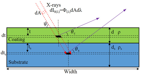
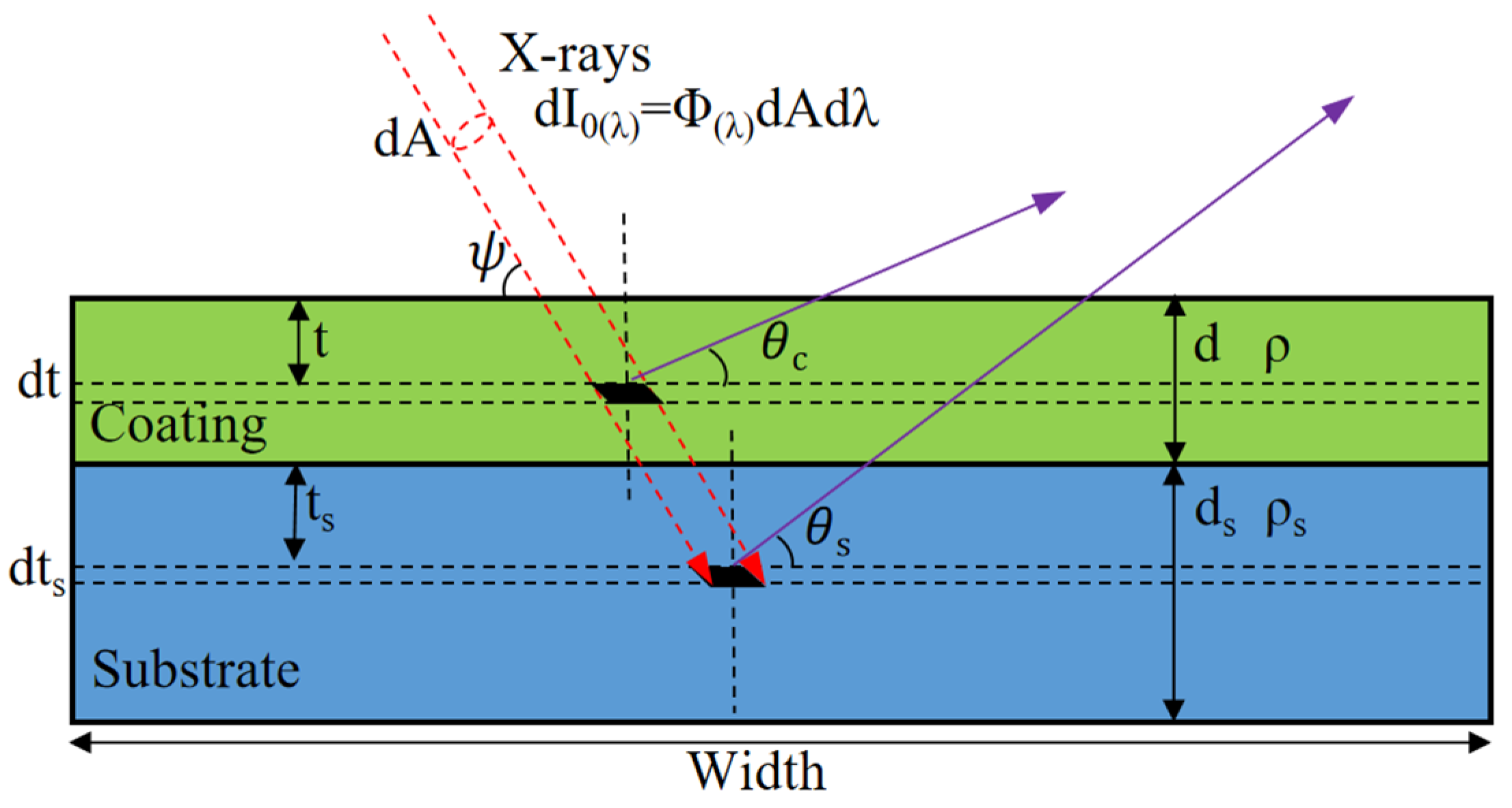
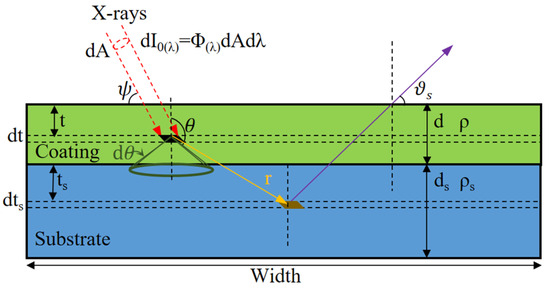
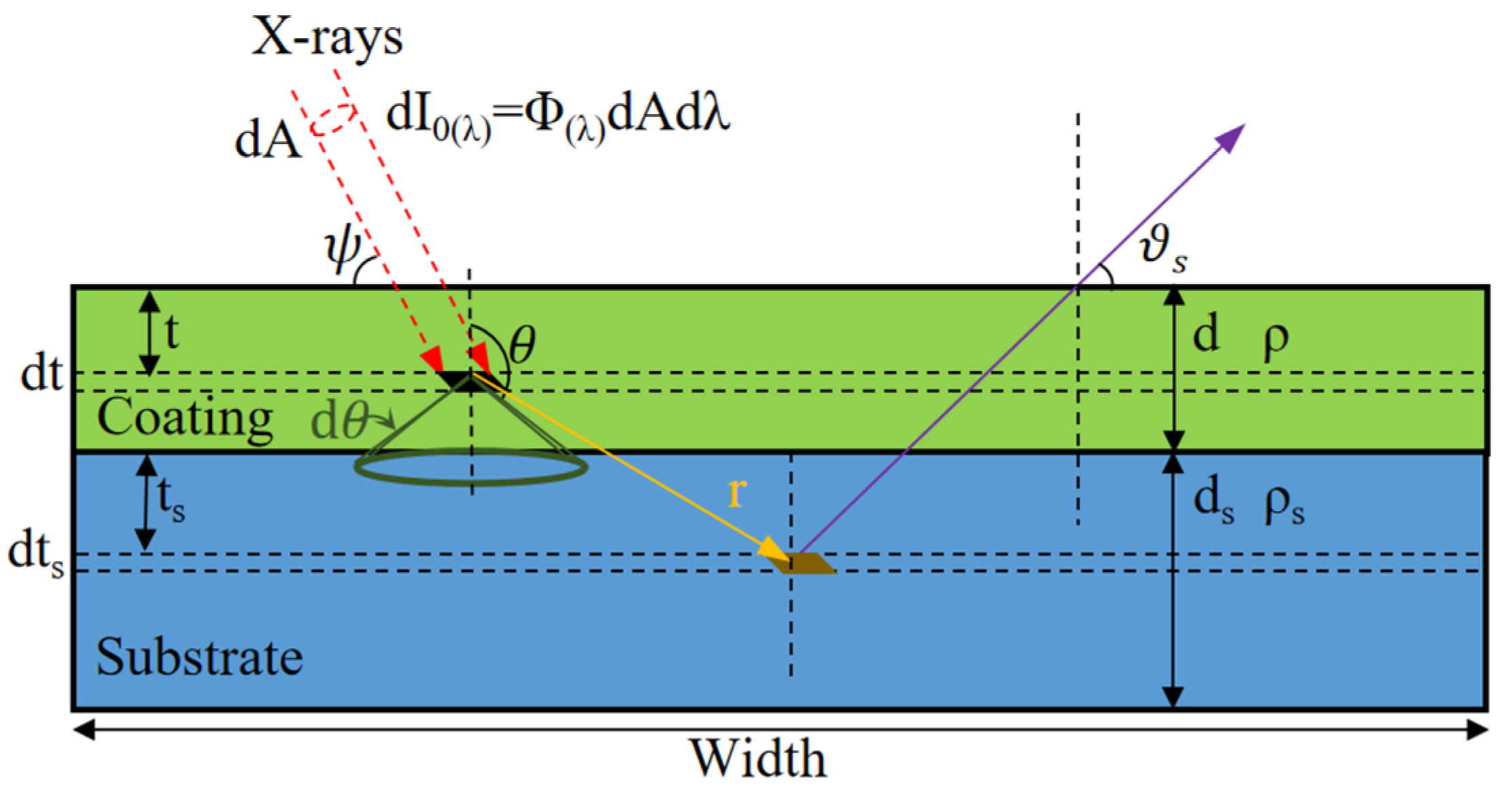
For the measurement of monolayer films, Figure 1 illustrates the excitation of primary fluorescence in the target element.

Figure 1. Schematic diagram of parallel X-rays with a wavelength λ incident on a monolayer film sample, exciting the primary fluorescence of the target element.

The intensity and flux of incident X-rays with a wavelength $\lambda$ are denoted as $\mathrm{d}{\mathrm{I}}_0\left(\lambda \right)$ and $\Phi (\lambda )$, respectively. As X-rays pass through a homogeneous material, they interact with the atoms of the material via the photoelectric effect, Compton scattering, and Rayleigh scattering. Primary fluorescent photons are emitted when the X-rays are photoelectrically absorbed by elements. Consequently, the primary fluorescent intensities recorded by the detector from the coating and the substrate are denoted as ${\mathrm{I}}_{\mathrm{c},1}$ and ${\mathrm{I}}_{\mathrm{s},1}$, respectively, as expressed in Equations (1) and (2).

$${\mathrm{I}}_{\mathrm{c},1}=(\csc \psi {\displaystyle \frac{\Omega }{4\pi }}{\epsilon }_{\mathrm{c},\mathrm{i}}){\mathrm{E}}_{\mathrm{c},\mathrm{i}}{\mathrm{C}}_{\mathrm{c},\mathrm{i}}{\int }_{{\lambda }_{\min }}^{{\lambda }_{\mathrm{ab},\mathrm{i}}}{\displaystyle \frac{{\mathrm{I}}_0\left(\lambda \right){\tau }_{\mathrm{c},\mathrm{i},\lambda }}{{\mu }_{\mathrm{c}}^{*}}}(1-{\mathrm{e}}^{-{\mu }_{\mathrm{c}}^{*}\rho \mathrm{d}})\mathrm{d}\lambda$$

(1)

$${\mu }_{\mathrm{c}}^{*}={ \mu }_{\mathrm{c},\lambda }\csc \psi +{\mu }_{\mathrm{c},\lambda \mathrm{i}}\csc {\theta }_{\mathrm{c}},{\mathrm{E}}_{\mathrm{c},\mathrm{i}}={ \mathrm{J}}_{\mathrm{c},\mathrm{i}}{\omega }_{\mathrm{c},\mathrm{i}}{\mathrm{f}}_{\mathrm{c},\mathrm{i}}$$

$${\mathrm{I}}_{\mathrm{s},1}={\mathrm{e}}^{-{\mu }_{\mathrm{c},\lambda \mathrm{j}}\rho \mathrm{dcsc}{\theta }_{\mathrm{s}}}(\csc \psi {\displaystyle \frac{\Omega }{4\pi }}{\epsilon }_{\mathrm{s},\mathrm{j}}){\mathrm{E}}_{\mathrm{s},\mathrm{j}}{\mathrm{C}}_{\mathrm{s},\mathrm{j}}{\int }_{{\lambda }_{\min }}^{{\lambda }_{\mathrm{ab},\mathrm{j}}}{\mathrm{e}}^{-{\mu }_{\mathrm{c},\lambda }\rho \mathrm{dcsc}\psi }{\displaystyle \frac{{\mathrm{I}}_0\left(\lambda \right){\tau }_{\mathrm{s},\mathrm{j},\lambda }}{{\mu }_{\mathrm{s}}^{*}}}(1-{\mathrm{e}}^{-{\mu }_{\mathrm{s}}^{*}{\rho }_{\mathrm{s}}{\mathrm{d}}_{\mathrm{s}}})\mathrm{d}\lambda$$

(2)

$${\mu }_{\mathrm{s}}^{*}={\mu }_{\mathrm{s},\lambda }\csc \psi +{\mu }_{\mathrm{s},\lambda \mathrm{j}}\csc {\theta }_{\mathrm{s}},{\mathrm{E}}_{\mathrm{j} }={\mathrm{J}}_{\mathrm{s},\mathrm{j}}{\omega }_{\mathrm{s},\mathrm{j}}{\mathrm{f}}_{\mathrm{s},\mathrm{j}}$$

Here, $\mathrm{d}$ and ${\mathrm{d}}_{\mathrm{s}}$ are the thicknesses of the coating and the substrate, respectively; $\rho$ and ${\rho }_{\mathrm{s}}$ are their densities. ${\mathrm{C}}_{\mathrm{c},\mathrm{i}}$ and ${\mathrm{C}}_{\mathrm{c},\mathrm{i}}$ represent the concentrations of the target element in the coating and the substrate. ${\mu }_{\mathrm{c},\lambda }$ and ${\mu }_{\mathrm{s},\lambda }$ denote the mass absorption coefficients of the coating and the substrate for X-rays with a wavelength $\lambda$. ${\mu }_{\mathrm{c},\lambda \mathrm{i}}$ is the mass absorption coefficient of the coating for the characteristic rays of target element i with a wavelength ${\lambda }_{\mathrm{i}}$. Similarly, ${\mu }_{\mathrm{s},\lambda \mathrm{j}}$ corresponds to the substrate and element j. ${\tau }_{\mathrm{c},\mathrm{i},\lambda }$ and ${\tau }_{\mathrm{s},\mathrm{j},\lambda }$ are the mass photoelectric absorption coefficients of the target element for incident X-rays of wavelength lambda. $\psi$ is the angle between the incident ray and the sample surface, ${\theta }_{\mathrm{c}}$ and ${\theta }_{\mathrm{s}}$ are the angles between the emergent ray and the sample coating surface and substrate surface, respectively. ${\lambda }_{\min }$ is the minimum wavelength of the primary spectrum, while ${\lambda }_{\mathrm{ab},\mathrm{i}}$ and ${\lambda }_{\mathrm{ab},\mathrm{j}}$ are the maximum wavelengths in the primary spectrum capable of exciting the target elements in the coating and substrate, respectively, via the photoelectric effect. This process is determined by the absorption jump factor $\mathrm{J}$, fluorescence yield $\omega$, and transition probability $\mathrm{f}$. Finally, these fluorescent photons are detected over a solid angle Ω with a detection efficiency $\epsilon$. The detailed derivation process can be referred to in our previous work [25].

For a sufficiently thick coating $\mathrm{d}$, Equation (1) simplifies to Equation (3), while for a sufficiently thick substrate ${\mathrm{d}}_{\mathrm{s}}$, Equation (2) simplifies to Equation (4).

$${\mathrm{I}}_{\mathrm{c},1,\mathrm{d}\to \infty }=(\csc \psi {\displaystyle \frac{\Omega }{4\pi }}{\epsilon }_{\mathrm{c},\mathrm{i}}){\mathrm{E}}_{\mathrm{c},\mathrm{i}}{\mathrm{C}}_{\mathrm{c},\mathrm{i}}{\int }_{{\lambda }_{\min }}^{{\lambda }_{\mathrm{ab},\mathrm{i}}}{\displaystyle \frac{{\mathrm{I}}_0\left(\lambda \right){\tau }_{\mathrm{c},\mathrm{i},\lambda }}{{\mu }_{\mathrm{c}}^{*}}}\mathrm{d}\lambda$$

(3)

$${\mathrm{I}}_{\mathrm{s},1,\mathrm{ds}\to \infty }={\mathrm{e}}^{-{\mu }_{\mathrm{c},\lambda \mathrm{j}}\rho \mathrm{dcsc}\theta }(\csc \psi {\displaystyle \frac{\Omega }{4\pi }}{\epsilon }_{\mathrm{s},\mathrm{j}}){\mathrm{E}}_{\mathrm{s},\mathrm{j}}{\mathrm{C}}_{\mathrm{s},\mathrm{j}}{\int }_{{\lambda }_{\min }}^{{\lambda }_{\mathrm{ab},\mathrm{j}}}{\mathrm{e}}^{-{\mu }_{\mathrm{c},\lambda }\rho \mathrm{dcsc}\psi }{\displaystyle \frac{{\mathrm{I}}_0\left(\lambda \right){\tau }_{\mathrm{s},\mathrm{j},\lambda }}{{\mu }_{\mathrm{s}}^{*}}}\mathrm{d}\lambda$$

(4)

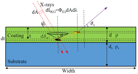
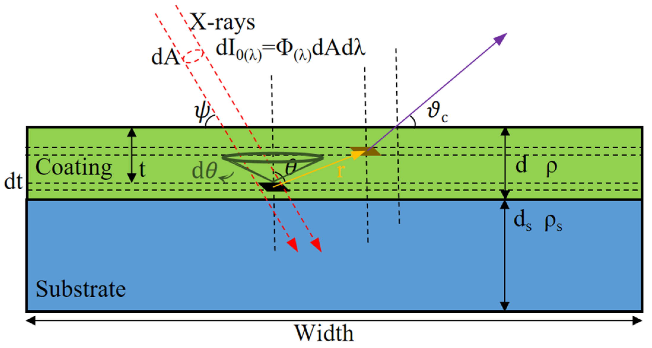
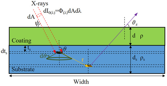
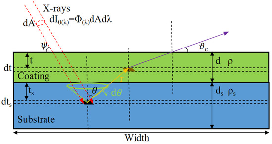
Secondary fluorescence can be produced within the same layer or across different layers [26,27]. The former involves characteristic photons being absorbed within their originating layer to induce secondary fluorescence, as illustrated in Figure 2 and Figure 3. The latter involves characteristic photons crossing at least one interlayer boundary before being absorbed by another layer, leading to secondary fluorescence there, as illustrated in Figure 4 and Figure 5.

Figure 2. The intralayer secondary fluorescent from the coating.

Figure 3. The intralayer secondary fluorescent from the substrate.

Figure 4. The interlayer secondary fluorescent from the coating.

Figure 5. The interlayer secondary fluorescent from the substrate.

The intralayer secondary fluorescent intensity ${\mathrm{I}}_{{\mathrm{i}}^{\prime }\to \mathrm{i}}$ of the target element $\mathrm{i}$ excited by element ${\mathrm{i}}^{\prime }$ in the coating is derived as Equation (5) below.

$${\mathrm{I}}_{{\mathrm{i}}^{\prime }\to \mathrm{i}}={\int }_{{\lambda }_{\min }}^{{\lambda }_{\mathrm{ab},{\mathrm{i}}^{\prime }}}{\int }_{\mathrm{t}=0}^{\mathrm{t}=\mathrm{d}}{\int }_{\mathrm{r}=0}^{{\mathrm{r}}_{\max }}{\int }_{\theta =0}^{\theta =\pi }{\mathrm{I}}_{\mathrm{i},\lambda }^{\prime }\mathrm{d}\theta \mathrm{drdtd}\lambda ,{\mathrm{r}}_{\max }=\left\{\begin{array}{c}{\displaystyle \frac{\mathrm{t}}{\cos \theta }} ,\theta <{\displaystyle \frac{\pi }{2}}\\ {\displaystyle \frac{\mathrm{d}-\mathrm{t}}{\cos (\pi -\theta )}},\theta > {\displaystyle \frac{\pi }{2}}\\ \mathrm{W}\mathrm{i}\mathrm{d}\mathrm{t}\mathrm{h} ,\theta ={\displaystyle \frac{\pi }{2}}\end{array}\right.$$

(5)

$${\mathrm{I}}_{\mathrm{i},\lambda }^{\prime }=[{\displaystyle \frac{1}{2}}{\mathrm{I}}_{{\mathrm{i}}^{\prime },\lambda }{\mathrm{e}}^{-{\mu }_{\mathrm{c},{\lambda }_{{\mathrm{i}}^{\prime }}}\rho \mathrm{r}}\sin \theta ]\left({\mathrm{C}}_{\mathrm{c},\mathrm{i}}\rho {\tau }_{\mathrm{c},\mathrm{i},{\lambda }_{{\mathrm{i}}^{\prime }}}\right)\left({\mathrm{J}}_{\mathrm{c},\mathrm{i}}{\omega }_{\mathrm{c},\mathrm{i}}{\mathrm{f}}_{\mathrm{c},\mathrm{i}}\right)[{\mathrm{e}}^{-{\mu }_{\mathrm{c},{\lambda }_{\mathrm{i}}}\rho (\mathrm{t}-\mathrm{rcos}\theta )/\sin {\mathsf{\vartheta }}_{\mathrm{c}}}]({\displaystyle \frac{\Omega }{4\pi }}{\epsilon }_{\mathrm{c},\mathrm{i}})$$

$${\mathrm{I}}_{{\mathrm{i}}^{\prime },\lambda }=[{\mathrm{I}}_0(\lambda ){\mathrm{e}}^{-{\mu }_{\mathrm{c},\lambda }\rho \mathrm{tcsc}\psi }]\left({\mathrm{C}}_{{\mathrm{c},\mathrm{i}}^{\prime }}\rho {\tau }_{{\mathrm{c},\mathrm{i}}^{\prime },\lambda }\csc \psi \right)\left({\mathrm{J}}_{{\mathrm{c},\mathrm{i}}^{\prime }}{\omega }_{{\mathrm{c},\mathrm{i}}^{\prime }}{\mathrm{F}}_{{\mathrm{c},\mathrm{i}}^{\prime }}\right)$$

The intralayer secondary fluorescent intensity ${\mathrm{I}}_{{\mathrm{j}}^{\prime }\to \mathrm{j}}$ of the target element $\mathrm{j}$ excited by element ${\mathrm{j}}^{\prime }$ in the substrate is derived as Equation (6) below.

$${\mathrm{I}}_{{\mathrm{j}}^{\prime }\to \mathrm{j}}={\mathrm{e}}^{-{\mu }_{\mathrm{c},\lambda \mathrm{j}}\rho \mathrm{dcsc}{\mathsf{\vartheta }}_{\mathrm{s}}}{\int }_{{\lambda }_{\min }}^{{\lambda }_{\mathrm{ab},{\mathrm{j}}^{\prime }}}{\int }_{{\mathrm{t}}_{\mathrm{s}}=0}^{{\mathrm{t}}_{\mathrm{s}}={\mathrm{d}}_{\mathrm{s}}}{\int }_{\mathrm{r}=0}^{{\mathrm{r}}_{\max }}{\int }_{\theta =0}^{\theta =\pi }{\mathrm{I}}_{\mathrm{j},\lambda }^{\prime }\mathrm{d}\theta \mathrm{drd}{\mathrm{t}}_{\mathrm{s}}\mathrm{d}\lambda ,{\mathrm{r}}_{\max }=\left\{\begin{array}{c}{\displaystyle \frac{{\mathrm{t}}_{\mathrm{s}}}{\cos \theta }} ,\theta <{\displaystyle \frac{\pi }{2}}\\ {\displaystyle \frac{{\mathrm{d}}_{\mathrm{s}}-{\mathrm{t}}_{\mathrm{s}}}{\cos (\pi -\theta )}}, \theta > {\displaystyle \frac{\pi }{2}}\\ \mathrm{W}\mathrm{i}\mathrm{d}\mathrm{t}\mathrm{h} ,\theta ={\displaystyle \frac{\pi }{2}}\end{array}\right.$$

(6)

$${\mathrm{I}}_{\mathrm{j},\lambda }^{\prime }=[{\displaystyle \frac{1}{2}}{\mathrm{I}}_{{\mathrm{j}}^{\prime },\lambda }{\mathrm{e}}^{-{\mu }_{\mathrm{s},{\lambda }_{{\mathrm{j}}^{\prime }}}{\rho }_{\mathrm{s}}\mathrm{r}}\sin \theta ]\left({\mathrm{C}}_{\mathrm{s},\mathrm{j}}{\rho }_{\mathrm{s}}{\tau }_{\mathrm{s},\mathrm{j},{\lambda }_{{\mathrm{j}}^{\prime }}}\right)\left({\mathrm{J}}_{\mathrm{s},\mathrm{j}}{\omega }_{\mathrm{s},\mathrm{j}}{\mathrm{f}}_{\mathrm{s},\mathrm{j}}\right)[{\mathrm{e}}^{-{\mu }_{\mathrm{s},{\lambda }_{\mathrm{j}}}{\rho }_{\mathrm{s}}({\mathrm{t}}_{\mathrm{s}}- \mathrm{rcos}\theta )/\sin {\mathsf{\vartheta }}_{\mathrm{s}}}]({\displaystyle \frac{\Omega }{4\pi }}{\epsilon }_{\mathrm{s},\mathrm{j}})$$

$${\mathrm{I}}_{\mathrm{j},\lambda }=[{\mathrm{I}}_0(\lambda ){\mathrm{e}}^{-({\mu }_{\mathrm{c},\lambda }\rho \mathrm{dcsc}\psi +{\mu }_{\mathrm{s},\lambda }{\rho }_{\mathrm{s}}{\mathrm{t}}_{\mathrm{s}}\csc \psi )}]\left({\mathrm{C}}_{{\mathrm{s},\mathrm{j}}^{\prime }}{\rho }_{\mathrm{s}}{\tau }_{{\mathrm{s},\mathrm{j}}^{\prime },\lambda }\csc \psi \right)\left({\mathrm{J}}_{{\mathrm{s},\mathrm{j}}^{\prime }}{\omega }_{{\mathrm{s},\mathrm{j}}^{\prime }}{\mathrm{F}}_{{\mathrm{s},\mathrm{j}}^{\prime }}\right)$$

The interlayer secondary fluorescent intensity ${\mathrm{I}}_{\mathrm{j}\to \mathrm{i}}$ of the target element $\mathrm{i}$ in coating excited by element $\mathrm{j}$ in the substrate is derived as Equation (7) below.

$${\mathrm{I}}_{\mathrm{j}\to \mathrm{i}}={\int }_{{\lambda }_{\min }}^{{\lambda }_{\mathrm{ab},\mathrm{j}}}{\int }_{\mathrm{t}=0}^{\mathrm{t}=\mathrm{d}}{\int }_{\theta =0}^{\theta =\pi }{\mathrm{I}}_{\mathrm{i},\lambda }^{\prime }\left({\mathrm{C}}_{\mathrm{c},\mathrm{i}}\rho {\tau }_{\mathrm{c},\mathrm{i},{\lambda }_{\mathrm{j}}}\right)\left({\mathrm{J}}_{\mathrm{c},\mathrm{i}}{\omega }_{\mathrm{c},\mathrm{i}}{\mathrm{f}}_{\mathrm{c},\mathrm{i}}\right){\mathrm{e}}^{-{\mu }_{\mathrm{c},{\lambda }_{\mathrm{i}}}\rho \mathrm{t}/\sin {\mathsf{\vartheta }}_{\mathrm{c}}}({\displaystyle \frac{\Omega }{4\pi }}{\epsilon }_{\mathrm{c},\mathrm{i}})\mathrm{d}\theta \mathrm{dtd}\lambda$$

(7)

$${\mathrm{I}}_{\mathrm{i},\lambda }^{\prime }={\int }_{{\mathrm{t}}_{\mathrm{s}}=0}^{{\mathrm{t}}_{\mathrm{s}}={\mathrm{d}}_{\mathrm{s}}}[{\displaystyle \frac{1}{2}}{\mathrm{I}}_{\mathrm{j},\lambda }{\mathrm{e}}^{-{[\mu }_{\mathrm{s},{\lambda }_{\mathrm{j}}}{\rho }_{\mathrm{s}}{\mathrm{t}}_{\mathrm{s}}\sec \theta +{\mu }_{\mathrm{c},{\lambda }_{\mathrm{j}}}\rho (\mathrm{r}-{\mathrm{t}}_{\mathrm{s}}\sec \theta )]}\sin \theta ]\mathrm{d}{\mathrm{t}}_{\mathrm{s}}, \mathrm{r}=\left\{\begin{array}{cc}\hfill {\displaystyle \frac{{\mathrm{t}}_{\mathrm{s}}+\mathrm{d}-\mathrm{t}}{\cos \theta }} & ,\theta < {\displaystyle \frac{\pi }{2}}\hfill \\ \hfill \mathrm{W}\mathrm{i}\mathrm{d}\mathrm{t}\mathrm{h} & ,\theta ={\displaystyle \frac{\pi }{2}}\hfill \end{array}\right.$$

$${\mathrm{I}}_{\mathrm{j},\lambda }=[{\mathrm{I}}_0(\lambda ){\mathrm{e}}^{-({\mu }_{\mathrm{c},\lambda }\rho \mathrm{dcsc}\psi +{\mu }_{\mathrm{s},\lambda }{\rho }_{\mathrm{s}}{\mathrm{t}}_{\mathrm{s}}\csc \psi )}]\left({\mathrm{C}}_{\mathrm{s},\mathrm{j}}{\rho }_{\mathrm{s}}{\tau }_{\mathrm{s},\mathrm{j},\lambda }\csc \psi \right)\left({\mathrm{J}}_{\mathrm{s},\mathrm{j}}{\omega }_{\mathrm{s},\mathrm{j}}{\mathrm{F}}_{\mathrm{s},\mathrm{j}}\right)$$

The interlayer secondary fluorescent intensity ${\mathrm{I}}_{\mathrm{i}\to \mathrm{j}}$ of the target element $\mathrm{j}$ in substrate excited by element $\mathrm{i}$ in the coating is derived as Equation (8) below.

$${\mathrm{I}}_{\mathrm{i}\to \mathrm{j}}={\int }_{{\lambda }_{\min }}^{{\lambda }_{\mathrm{ab},\mathrm{i}}}{\int }_{{\mathrm{t}}_{\mathrm{s} }=0}^{{\mathrm{t}}_{\mathrm{s}}={\mathrm{d}}_{\mathrm{s}}}{\int }_{\theta =0}^{\theta =\pi }{\mathrm{I}}_{\mathrm{j},\lambda }^{\prime }\left({\mathrm{C}}_{\mathrm{s},\mathrm{j}}{\rho }_{\mathrm{s}}{\tau }_{\mathrm{s},\mathrm{j},{\lambda }_{\mathrm{i}}}\right)\left({\mathrm{J}}_{\mathrm{s},\mathrm{j}}{\omega }_{\mathrm{s},\mathrm{j}}{\mathrm{f}}_{\mathrm{s},\mathrm{j}}\right){\mathrm{e}}^{-{\mu }_{\mathrm{s},{\lambda }_{\mathrm{j}}}{\rho }_{\mathrm{s}}{\mathrm{t}}_{\mathrm{s}}/\sin {\mathsf{\vartheta }}_{\mathrm{s}}}({\displaystyle \frac{\Omega }{4\pi }}{\epsilon }_{\mathrm{s},\mathrm{j}})\mathrm{d}\theta \mathrm{dtd}\lambda$$

(8)

$${\mathrm{I}}_{\mathrm{j},\lambda }^{\prime }={\int }_{\mathrm{t}=0}^{\mathrm{t}=\mathrm{d}}[{\displaystyle \frac{1}{2}}{\mathrm{I}}_{\mathrm{i},\lambda }{\mathrm{e}}^{{\mu }_{\mathrm{c},{\lambda }_{\mathrm{i}}}\rho \mathrm{tsec}\theta -{\mu }_{\mathrm{s},{\lambda }_{\mathrm{i}}}{\rho }_{\mathrm{s}}(\mathrm{r}+\mathrm{tsec}\theta )}\sin \theta ]\mathrm{dt}, \mathrm{r}=\left\{\begin{array}{c}{\displaystyle \frac{{\mathrm{t}}_{\mathrm{s}}+\mathrm{d}-\mathrm{t}}{\cos \theta }} ,\theta > {\displaystyle \frac{\pi }{2}}\\ \mathrm{W}\mathrm{i}\mathrm{d}\mathrm{t}\mathrm{h} ,\theta ={\displaystyle \frac{\pi }{2}}\end{array}\right.$$

$${\mathrm{I}}_{\mathrm{i},\lambda }=[{\mathrm{I}}_0(\lambda ){\mathrm{e}}^{-{\mu }_{\mathrm{c},\lambda }{\rho }_{\mathrm{c}}{\mathrm{t}}_{\mathrm{c}}\csc \psi }]\left({\mathrm{C}}_{\mathrm{c},\mathrm{i}}\rho {\tau }_{\mathrm{c},\mathrm{i},\lambda }\csc \psi \right)\left({\mathrm{J}}_{\mathrm{c},\mathrm{i}}{\omega }_{\mathrm{c},\mathrm{i}}{\mathrm{F}}_{\mathrm{c},\mathrm{i}}\right)$$

where ${\mathrm{I}}_{\mathrm{j},\lambda }$ is the characteristic X-ray intensity generated by element j in the substrate for incident X-rays of wavelength $\lambda$. ${\tau }_{\mathrm{s},\mathrm{j},\lambda }$ is the mass photoelectric absorption coefficient of element $\mathrm{j}$ in the substrate for incident X-rays of wavelength λ. ${\mu }_{\mathrm{s},{\lambda }_{\mathrm{j}}}$ is the mass absorption coefficient of the substrate for the characteristic X-rays of element $\mathrm{j}$. ${\mu }_{\mathrm{c},{\lambda }_{\mathrm{j}}}$ is the mass absorption coefficient of the coating for the characteristic X-rays of element $\mathrm{j}$. ${\tau }_{\mathrm{c},\mathrm{i},{\lambda }_{\mathrm{j}}}$ is the mass photoelectric absorption coefficient of element $\mathrm{i}$ in the coating for the characteristic X-rays of element j in the substrate. “Width” denotes the sample width. Similar definitions apply to Equation (8), with the positions of i and j interchanged.

Consider a scenario where the sample contains multiple elements (e.g., k, l, m, n, …, z) that can excite the target element via the same physical mechanism. In this case, the secondary fluorescence intensities from all contributing elements and all their characteristic spectral lines must be summed. Thus, the total interlayer secondary fluorescence intensity ${\mathrm{I}}_2$ detected from the coating and substrate is expressed by Equations (9) and (10) below.

$${\mathrm{I}}_{\mathrm{c},2}={\sum }_{ele.}{\sum }_{line}{\mathrm{I}}_{\mathrm{j}\to \mathrm{i}}$$

(9)

$${\mathrm{I}}_{\mathrm{s},2}={\sum }_{ele.}{\sum }_{line}{\mathrm{I}}_{\mathrm{i}\to \mathrm{j}}$$

(10)

Typically, tertiary fluorescence accounts for no more than 4% of the total fluorescence intensity; thus, tertiary and higher-order fluorescence can be neglected. Only the primary and secondary fluorescence of the target element are considered in this study [27]. Accordingly, the total fluorescence intensity detected from the coating and substrate is the sum of the primary and secondary fluorescence photon intensities, as given by Equations (11) and (12) below.

$${\mathrm{I}}_{\mathrm{c}}={\mathrm{I}}_{\mathrm{c},1}+{\mathrm{I}}_{\mathrm{c},2}$$

(11)

$${\mathrm{I}}_{\mathrm{s}}={\mathrm{I}}_{\mathrm{s},1}+{\mathrm{I}}_{\mathrm{s},2}$$

(12)

When the target element of interest exists in both the coating and the substrate, the corresponding expression is given by Equation (13) below.

$$\mathrm{I}={ \mathrm{I}}_{\mathrm{c}}+{\mathrm{I}}_{\mathrm{s}}$$

(13)

To reduce the impact of uncertainties in detection efficiency, fluorescence excitation factor, and absorption coefficient on thickness calculation results, relative intensity (RI) is used to represent the fluorescence intensity. The relative intensities of characteristic fluorescence from the coating and substrate are given by Equations (14) and (15), respectively.

$$\mathrm{RI}(\mathrm{coa}.)={\displaystyle \frac{{\mathrm{I}}_{\mathrm{c}}}{(\csc \psi \frac{\Omega }{4\pi }{\epsilon }_{\mathrm{c},\mathrm{i}}){\mathrm{E}}_{\mathrm{c},\mathrm{i}}{\int }_{{\lambda }_{\min }}^{{\lambda }_{\mathrm{ab},\mathrm{i}}}\frac{{\mathrm{I}}_0\left(\lambda \right){\tau }_{\mathrm{c},\mathrm{i},\lambda }}{{\mu }_{\mathrm{c}}^{*}}\mathrm{d}\lambda }}$$

(14)

$$\mathrm{RI}(\mathrm{sub}.)={\displaystyle \frac{{\mathrm{I}}_{\mathrm{s}}}{ (\csc \psi \frac{\Omega }{4\pi }{\epsilon }_{\mathrm{s},\mathrm{j}}){\mathrm{E}}_{\mathrm{s},\mathrm{j}}{\int }_{{\lambda }_{\min }}^{{\lambda }_{\mathrm{ab},\mathrm{j}}}\frac{{\mathrm{I}}_0\left(\lambda \right){\tau }_{\mathrm{s},\mathrm{j},\lambda }}{{\mu }_{\mathrm{s}}^{*}}\mathrm{d}\lambda }}$$

(15)

2.3. Correlation Between Characteristic X-Ray Intensity and Coating Thickness

In this work, FP-EDXRF was employed to determine the surface coating thickness of Zr alloy samples. This method is based on fundamental physical parameters and rigorous theoretical formulations of X-ray fluorescence intensity [28,29]. First, it calculates the theoretical intensity. Next, the method compares this theoretical value with the actual measured intensity. Finally, the thickness is continuously corrected using an iterative formula until the preset accuracy requirement is met [30,31].

The RI of the Zr K_α ray in the Cr-coated sample can be obtained from Equation (16). The numerator corresponds to the total fluorescence intensity of Zr K_α from the actual sample. Since the Cr coating contains no Zr, interlayer secondary fluorescence is neglected. The denominator refers to that from a pure Zr sample. By combining the fluorescence theoretical formula for the Zr K_α spectral line with the First Mean Value Theorem for Integrals, the simplified formula for the relative intensity of the Zr K_α spectral line can be derived as Equation (17).

$$\mathrm{R}{\mathrm{I}}_{\_\mathrm{Zr}{\mathrm{K}}_{\alpha }}={\displaystyle \frac{{\mathrm{I}}_{\mathrm{Zr}\text{-}4,\mathrm{Zr}{\mathrm{K}}_{\alpha }}}{(\csc \psi \frac{\Omega }{4\pi }{\epsilon }_{\mathrm{Zr},\mathrm{Zr}{\mathrm{K}}_{\alpha }}){\mathrm{E}}_{\mathrm{Zr}}{\int }_{{\lambda }_{\min }}^{{\lambda }_{\mathrm{ab},\mathrm{Zr}{\mathrm{K}}_{\alpha }}}\frac{{\mathrm{I}}_0\left(\lambda \right){\tau }_{\mathrm{Zr},\lambda }}{{\mu }_{\mathrm{Zr}}^{*}}\mathrm{d}\lambda }}$$

(16)

$${\mu }_{\mathrm{Zr}}^{*}={ \mu }_{\mathrm{Zr},\lambda }\csc \psi +{\mu }_{\mathrm{Zr},\mathrm{Zr}{\mathrm{K}}_{\alpha }}\csc \theta , {\mathrm{E}}_{\mathrm{Zr}}={\mathrm{J}}_{\mathrm{Zr},\mathrm{Zr}{\mathrm{K}}_{\alpha }}{\omega }_{\mathrm{Zr},\mathrm{Zr}{\mathrm{K}}_{\alpha }}{\mathrm{f}}_{\mathrm{Zr},\mathrm{Zr}{\mathrm{K}}_{\alpha }}$$

$$\mathrm{R}{\mathrm{I}}_{\_\mathrm{Zr}{\mathrm{k}}_{\alpha }} \approx {\displaystyle \frac{{\mathrm{e}}^{-{\mu }_{\mathrm{Cr},\mathrm{Zr}{\mathrm{K}}_{\alpha }}\rho \mathrm{dcsc}\theta }{\mathrm{C}}_{\mathrm{Zr}\text{-}4,\mathrm{Zr}{\mathrm{K}}_{\alpha }}{\int }_{{\lambda }_{\min }}^{{\lambda }_{\mathrm{ab},\mathrm{Zr}{\mathrm{K}}_{\alpha }}}{\mathrm{e}}^{-{\mu }_{\mathrm{Cr},\lambda }\rho \mathrm{dcsc}\psi }\frac{{\mathrm{I}}_0\left(\lambda \right){\tau }_{\mathrm{Zr}\text{-}4,\lambda }}{{\mu }_{\mathrm{Zr}\text{-}4}^{*}}\mathrm{d}\lambda }{{\int }_{{\lambda }_{\min }}^{{\lambda }_{\mathrm{ab},\mathrm{Zr}{\mathrm{K}}_{\alpha }}}\frac{{\mathrm{I}}_0\left(\lambda \right){\tau }_{\mathrm{Zr},\lambda }}{{\mu }_{\mathrm{Zr}}^{*}}\mathrm{d}\lambda }}$$

(17)

$$\approx {\mathrm{C}}_{\mathrm{Zr}\text{-}4,\mathrm{Zr}{\mathrm{K}}_{\alpha }}{\mathrm{e}}^{-\overline{{\mu }_1^{*}}\rho \mathrm{d}}=\alpha {\mathrm{e}}^{-\beta \mathrm{d}}$$

$${\mu }_{\mathrm{Zr}\text{-}4 }^{*}={\mu }_{\mathrm{Zr}\text{-}4,\lambda }\csc \psi +{\mu }_{{\mathrm{Z}}_{\mathrm{r}}\text{-}4,\mathrm{Zr}{\mathrm{K}}_{\alpha }}\csc \theta , {\mathrm{E}}_{\mathrm{Zr}\text{-}4}={\mathrm{J}}_{\mathrm{Zr}\text{-}4,\mathrm{Zr}{\mathrm{K}}_{\alpha }}{\omega }_{\mathrm{Zr}\text{-}4,\mathrm{Zr}{\mathrm{K}}_{\alpha }}{\mathrm{f}}_{\mathrm{Zr}\text{-}4,\mathrm{Zr}{\mathrm{K}}_{\alpha }}$$

where ${\mathrm{e}}^{-\overline{{\mu }_1^{*}}\rho \mathrm{d}}$ is the weighted mean function value. Calculating coating thickness involves nonlinear relationships, such as the exponential attenuation term, and lacks a direct analytical solution. Furthermore, measurement errors, model inaccuracies, and potential parameter coupling effects exist. Therefore, an iterative method is adopted to gradually correct the thickness value. Specifically, the current result is compared with the measured value. Repeated adjustments are then performed to approach the true value. The iterative correction formula for the coating thickness $\mathrm{d}$ is given by Equation (18).

$${\mathrm{d}}^{\prime }=\mathrm{d}{\displaystyle \frac{\ln (\mathrm{R}{\mathrm{I}}_{\mathrm{cm}\_\mathrm{Zr}{\mathrm{K}}_{\alpha }})}{\ln (\mathrm{R}{\mathrm{I}}_{\mathrm{cal}\_\mathrm{Zr}{\mathrm{K}}_{\alpha }})}}$$

(18)

where $\mathrm{R}{\mathrm{I}}_{\mathrm{cal}\_\mathrm{Zr}{\mathrm{K}}_{\alpha }}$ is the calculated value of RI during iteration. $\mathrm{R}{\mathrm{I}}_{\mathrm{cm}\_\mathrm{Zr}{\mathrm{K}}_{\alpha }}$ is the corrected measured value of RI, which is calculated according to Equation (19).

$$\mathrm{R}{\mathrm{I}}_{\mathrm{cm}\_\mathrm{Zr}{\mathrm{k}}_{\alpha }}={\displaystyle \frac{\mathrm{a}·{\mathrm{I}}_{\mathrm{mea}\_\mathrm{sam}\_\mathrm{Zr}{\mathrm{K}}_{\alpha }}+\mathrm{b}}{\mathrm{a}·{\mathrm{I}}_{\mathrm{mea}\_\mathrm{pbs}\_\mathrm{Zr}{\mathrm{K}}_{\alpha }}+\mathrm{b}}}$$

(19)

Here, ${\mathrm{I}}_{\mathrm{mea}\_\mathrm{sam}\_\mathrm{Zr}{\mathrm{K}}_{\alpha }}$ is the measured Zr K_α fluorescence intensity of the unknown sample. ${\mathrm{I}}_{\mathrm{mea}\_\mathrm{pbs}\_\mathrm{Zr}{\mathrm{K}}_{\alpha }}$ is the measured Zr K_α fluorescence intensity of the pure Zr bulk. $\mathrm{a}$ and $\mathrm{b}$ are the linear calibration parameters for the measured and theoretical fluorescence intensities of standard samples, derived from Equation (20).

$${\mathrm{I}}_{\mathrm{cm}\_\mathrm{std}}={\mathrm{I}}_{\mathrm{cal}\_\mathrm{std}}=\mathrm{a}·{\mathrm{I}}_{\mathrm{mea}\_\mathrm{std}}+\mathrm{b}$$

(20)

${\mathrm{I}}_{\mathrm{cm}\_\mathrm{std}}$ is the corrected measured fluorescence intensity of the standard sample. ${\mathrm{I}}_{\mathrm{cal}\_\mathrm{std}}$ is the theoretical fluorescence intensity of the standard sample. ${\mathrm{I}}_{\mathrm{mea}\_\mathrm{std}}$ is the measured fluorescence intensity of the standard sample.

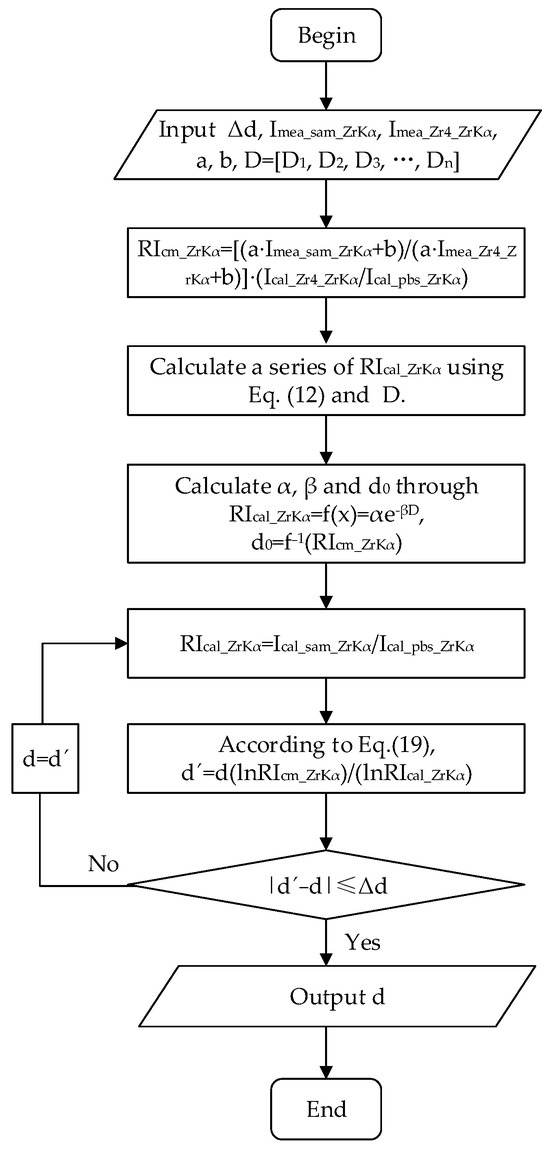
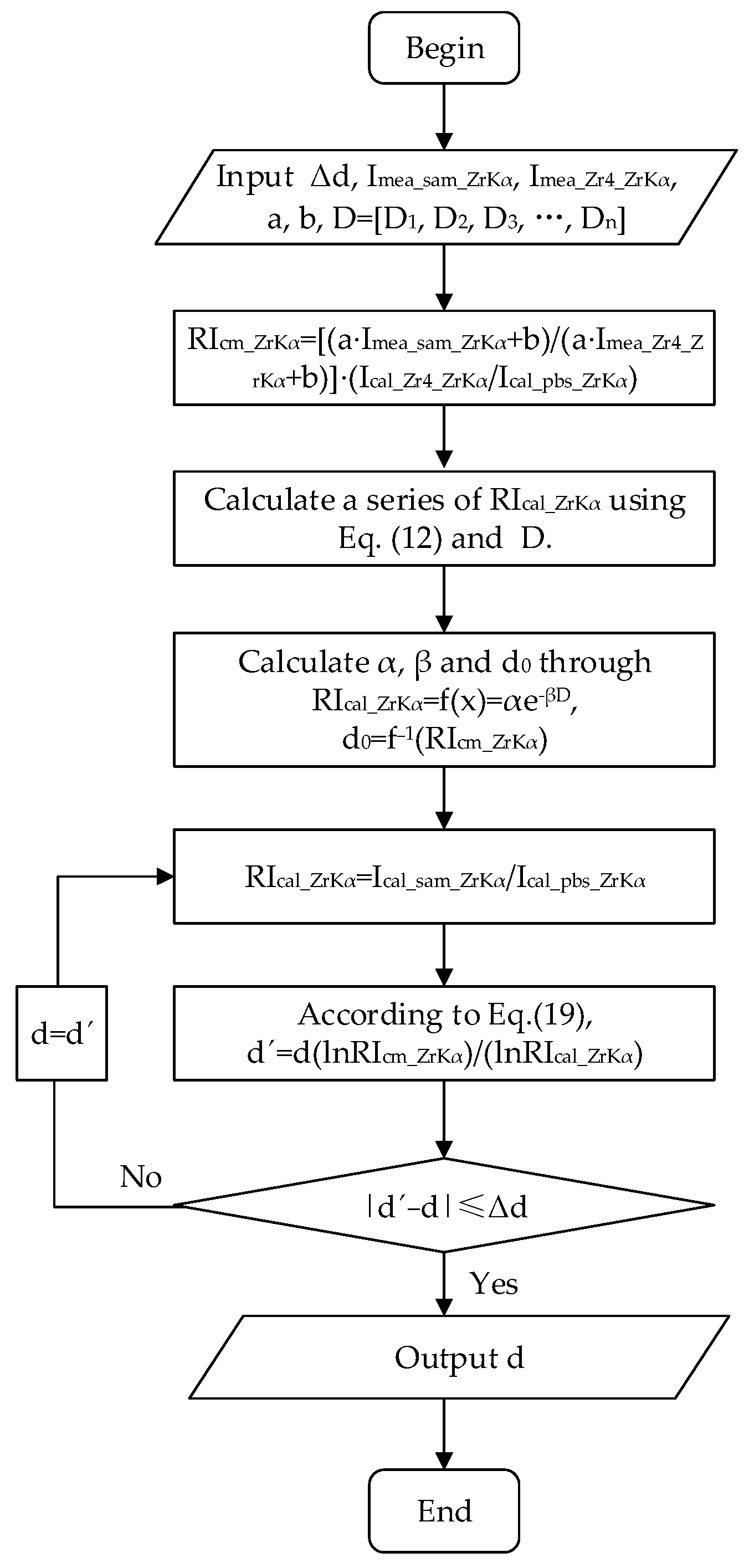
In this work, Python was used for programming implementation. The thickness of the Cr coating on was calculated iteratively via the fundamental parameter method, and a simplified flowchart of the algorithm is presented in Figure 6.

Figure 6. Iterative flowchart for the fundamental parameter method of EDXRF. $∆\mathrm{d}$ is the convergence limit of the calculated thickness of the coating. ${\mathrm{I}}_{\mathrm{mea}\_\mathrm{Zr}4\_\mathrm{Zr}{\mathrm{K}}_{\alpha }}$ is the measured Zr K_α fluorescence intensity of the Zr-4 bulk (i.e., the sample back side in the experiment). ${\mathrm{d}}_0$ is the initially calculated thickness value of the coating. D is a matrix consisting of a series of arbitrary thickness values. ${\mathrm{d}}^{\prime }$ is the updated calculated value of the coating thickness. In this work, the substrate of the sample has a thickness of 2 mm, which can be regarded as infinitely thick.

Step 1: Input the convergence limit ($∆\mathrm{d}$) of the calculated thickness of the coating; the measured fluorescence intensity (${\mathrm{I}}_{\mathrm{mea}\_\mathrm{sam}\_\mathrm{Zr}{\mathrm{K}}_{\alpha }}$) of Zr K_α from the unknown sample; the measured fluorescence intensity (${\mathrm{I}}_{\mathrm{mea}\_\mathrm{Zr}4\_\mathrm{Zr}{\mathrm{K}}_{\alpha }}$) of Zr K_α from the Zr-4 substrate; the linear calibration parameters a and b; and the matrix D composed of a series of coating thickness values (covering the thickness range of the unknown sample and meeting the requirements of statistical fitting).

Step 2: Based on the linear calibration parameters a and b, the calibrated measured value of relative fluorescence intensity ($\mathrm{R}{\mathrm{I}}_{\mathrm{cm}\_\mathrm{Zr}{\mathrm{K}}_{\alpha }}$) for the unknown sample was calculated to reduce instrumental systematic errors and interference from the testing environment.

Step 3: According to Equation (16), the theoretical values of relative fluorescence intensity (${\mathrm{RI}}_{\mathrm{cal}\_\mathrm{Zr}{\mathrm{K}}_{\alpha }}$) corresponding to each coating thickness value in matrix D were calculated, so as to establish a quantitative correlation between thickness and fluorescence intensity.

Step 4: The thickness-fluorescence intensity was fitted by Equation (17) to obtain the model parameters α and β. The calibrated measured value of relative fluorescence intensity ($\mathrm{R}{\mathrm{I}}_{\mathrm{cm}\_\mathrm{Zr}{\mathrm{K}}_{\alpha }}$) for the unknown sample is substituted into the model to obtain its initial calculated coating thickness (${\mathrm{d}}_0$), and the initial iterative value was set as $\mathrm{d} = {\mathrm{d}}_0$.

Step 5: According to Equation (16), the theoretical values of relative fluorescence intensity (${\mathrm{RI}}_{\mathrm{cal}\_\mathrm{Zr}{\mathrm{K}}_{\alpha }}$) corresponding to the current iterative thickness d was calculated.

Step 6: Combined with the calibrated measured relative fluorescence intensity ($\mathrm{R}{\mathrm{I}}_{\mathrm{cm}\_\mathrm{Zr}{\mathrm{K}}_{\alpha }}$) and the theoretical relative fluorescence intensity (${\mathrm{I}}_{\mathrm{cal}\_\mathrm{Zr}{\mathrm{K}}_{\alpha }}$) corresponding to the iterative thickness d, the updated coating thickness value (${\mathrm{d}}^{\prime }$) was calculated through Equation (18).

Step 7: If the absolute error between the updated thickness ${\mathrm{d}}^{\prime }$ and the current iterative thickness $\mathrm{d}$ is less than or equal to $∆\mathrm{d}$, the iteration is considered to converge, and the final calculated coating thickness $\mathrm{d}$ is output. If the absolute error is greater than the convergence threshold, set $\mathrm{d}={\mathrm{d}}^{\prime }$ and return to Step 5 to continue the iteration until the convergence condition is satisfied.

3. Experiments

3.1. Measurement Device

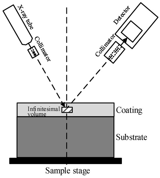
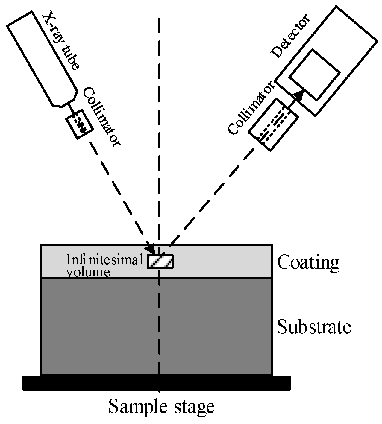
In this study, EDXRF measurements were performed using a self-developed system. This system consists of a silver (Ag)-anode X-ray tube with a tube operated at voltage of 30 kV, a Si-PIN semiconductor detector with an energy resolution of 196 eV (at ⁵⁵Fe), a detector collimator, an X-ray tube collimator, a sample stage, and electronic components for data acquisition and processing, as shown in Figure 7.

Figure 7. Schematic of the EDXRF measurement system structure.

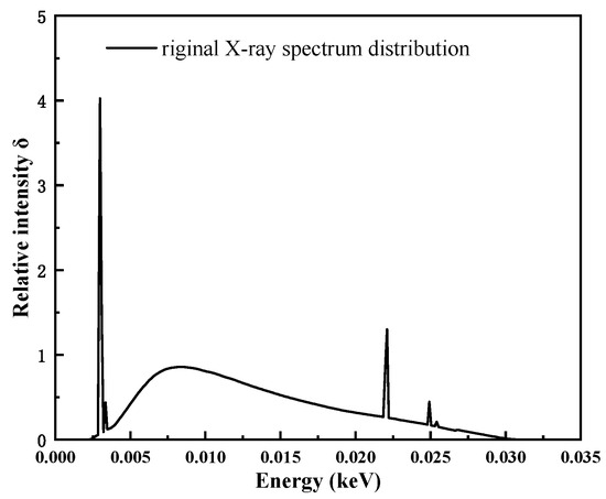
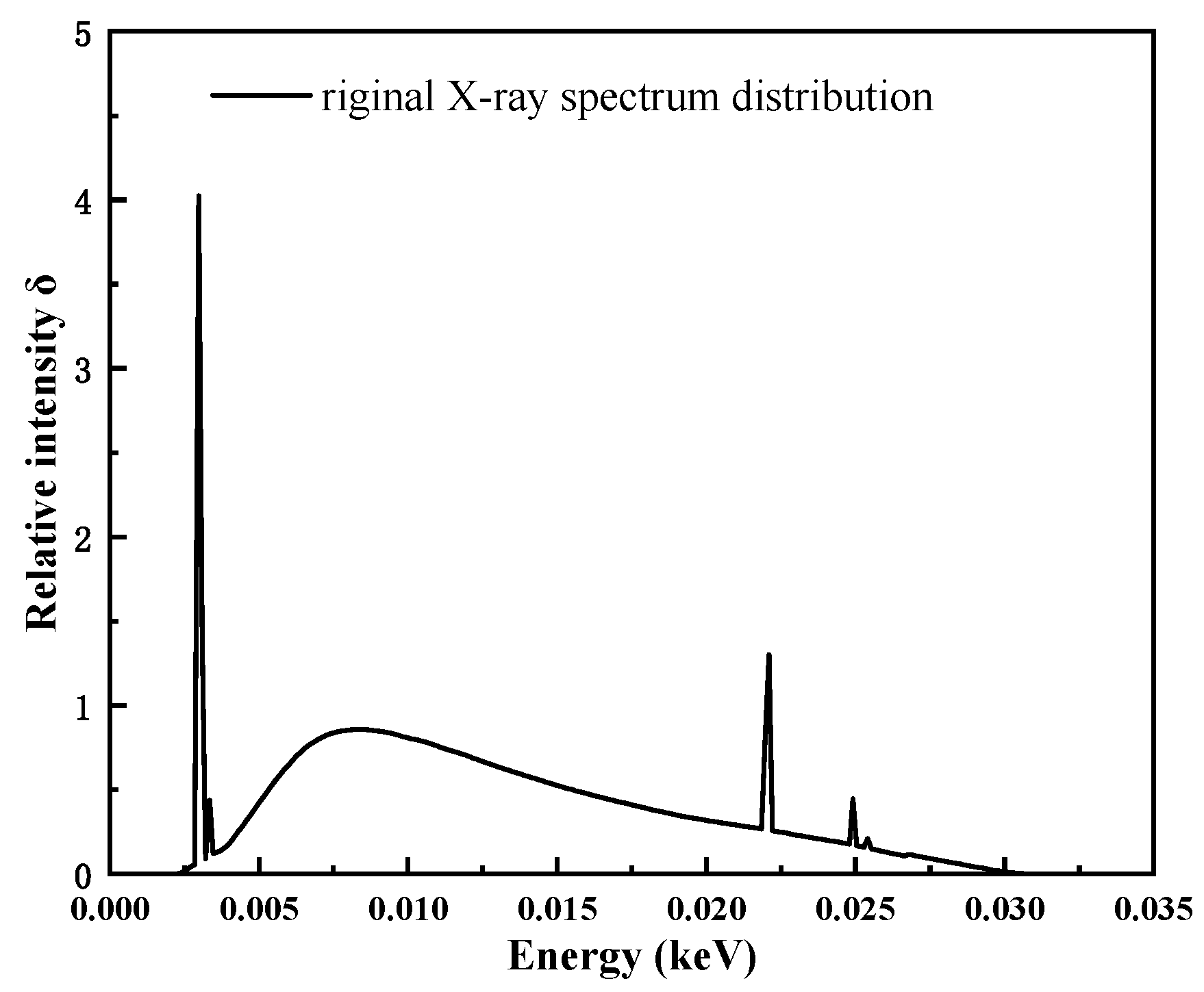
Electrons in the X-ray tube are accelerated to 30 keV; then, bombard a silver (Ag) target, generating primary X-rays with a continuous spectral distribution, including bremsstrahlung and characteristic X-rays, as shown in Figure 8. Notably, distinct characteristic peaks of Ag can be observed in the spectrum, including K_α (~22.1 keV), K_β (~24.9 keV), L_α (~2.9 keV), and L_β (~3.1 keV). In general, the lower the absorption edge energy, the easier it is to excite the characteristic X-rays of the corresponding series. For each sample, the measurement time was set to 5 min, and both the coated side and the back side (substrate) of each sample were measured three times, with the average value calculated.

Figure 8. Original X-ray spectral distribution of silver target.

3.2. Experiment Process

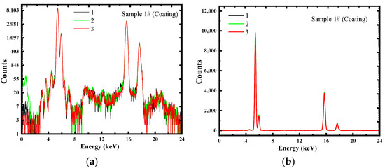
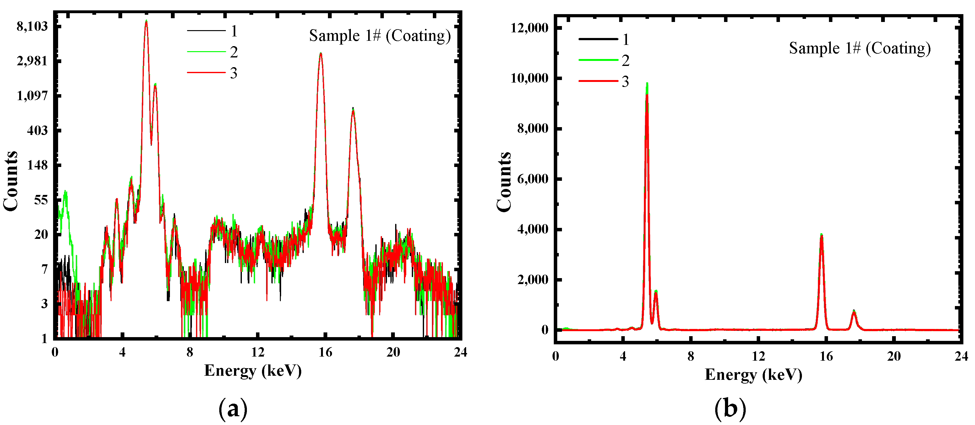
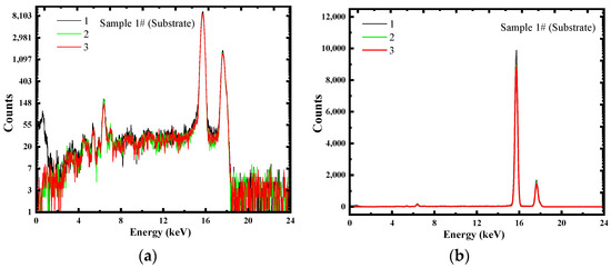
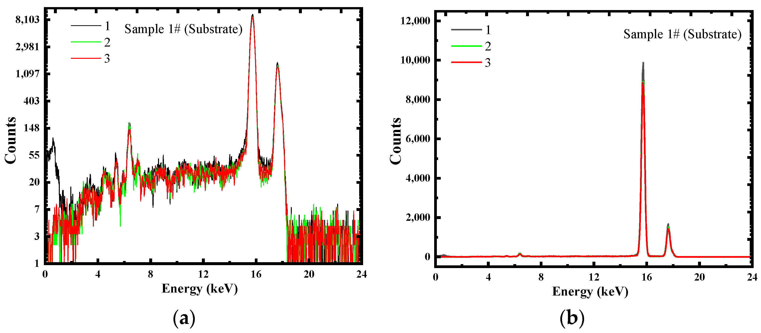
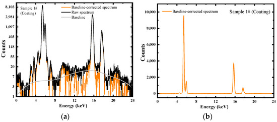
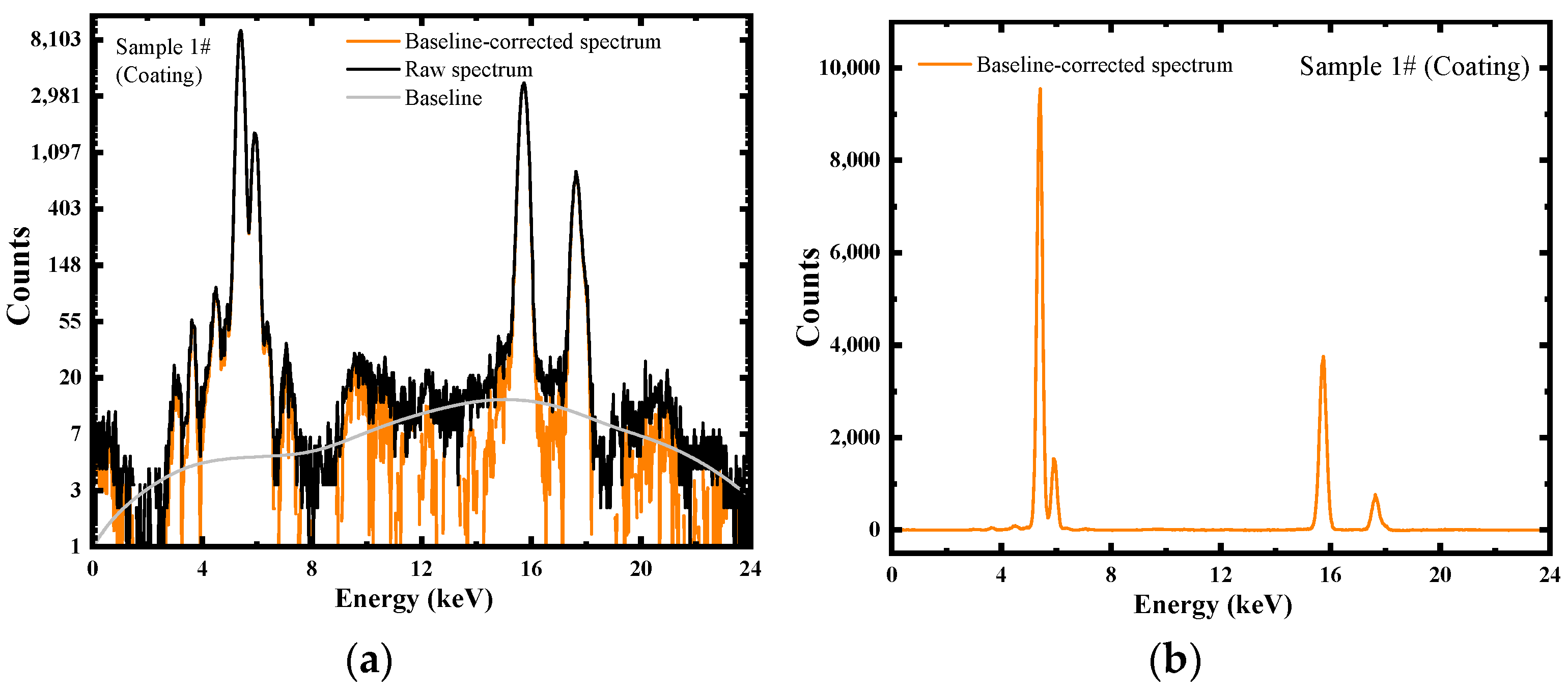
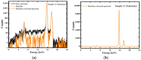
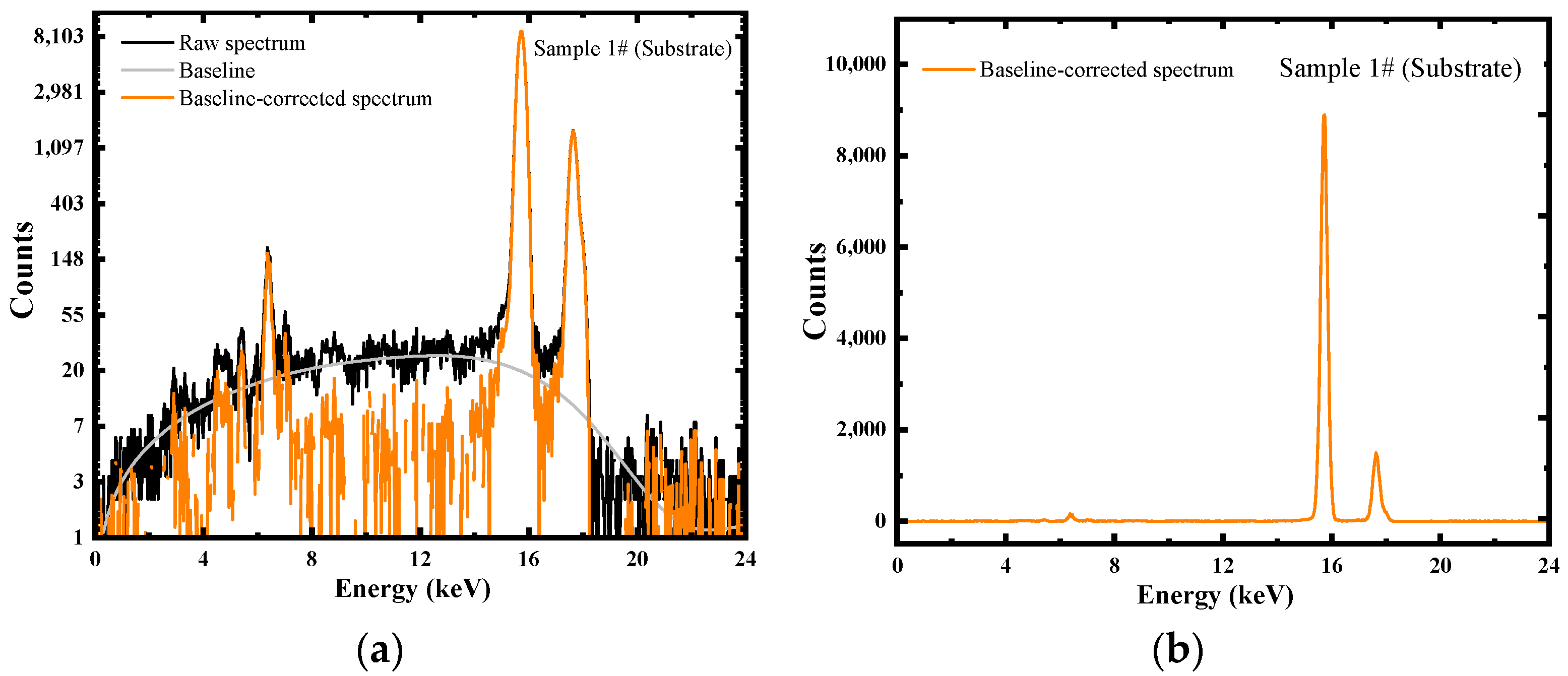
The original spectra of the coated sample 1# are shown in Figure 9a,b. Within the energy range of 4–8 keV, distinct characteristic K_α (~5.4 keV) and K_β (~5.9 keV) peaks of Cr can be observed. Meanwhile, in the range of 14–20 keV, obvious characteristic K_α (~15.7 keV) and K_β (~17.6 keV) peaks of Zr are present. The original spectra of the back side of sample 1# are displayed in Figure 10a,b. Only tiny characteristic peaks of Cr are found, with a photon count as low as 148, originating from the primary and secondary fluorescence of Cr element inherently present in the Zr alloy. In the range of 14–20 keV, distinct characteristic peaks of Zr are observed as well, and the photon count increases significantly, with the maximum value reaching approximately 10,000.

Figure 9. Raw energy spectra of sample 1# (coated side) from three same measurements. (a) Ordinate presented on an ‘Ln’ (natural logarithm) scale; (b) Ordinate presented on a linear scale.

Figure 10. Raw energy spectra of sample 1# (back side) from three same measurements. (a) Ordinate presented on an ‘Ln’ (natural logarithm) scale; (b) Ordinate presented on a linear scale.

In EDXRF analysis, baseline correction—the first step in spectral analysis—is crucial as it ensures the accuracy of subsequent procedures, including multi-peak analysis and content quantification. By appropriately selecting baseline data points for spectral fitting, the baseline can be accurately estimated [32]. Figure 11 and Figure 12 show the spectra of the coated side and the back side of sample 1# after baseline subtraction and baseline correction, respectively.

Figure 11. Data procession of sample 1# (coated side). (a) Baseline; (b) Baseline-corrected spectrum.

Figure 12. Data procession of sample 1# (back side). (a) Baseline; (b) Baseline-corrected spectrum.

Due to the distinct elemental difference between the substrate and the coating, they can be distinguished by comparing the Zr fluorescence intensity. After obtaining the baseline-corrected energy spectrum, it is necessary to first determine the position of the Zr K_α characteristic peak, then identify its boundaries (defined as the positions where the intensity fluctuates within the baseline range), and subsequently calculate the peak area of this characteristic peak. This peak area serves as a key basis for subsequent analysis. Table 3 presents the relative intensities of all samples, the average counts of the Zr K_α characteristic peak on the coated side and back side, and the relative deviation. The standard deviation of the average counts is calculated using the error propagation formula ${\mathsf{\sigma }}_{\overline{\mathrm{I}}}=\sqrt{\overline{\mathrm{I}}/\mathrm{k}}$ where $\overline{\mathrm{I}}={\displaystyle \frac{1}{\mathrm{k}}}\sum _{\mathrm{i}=1}^{\mathrm{k}}{\mathrm{I}}_{\mathrm{i}}$, $\mathrm{k}$ represents the number of measurements and ${\mathrm{I}}_{\mathrm{i}}$ is the fluorescence intensity of each measurement.

Table 3. The relative intensities of all samples, as well as the average counts of the characteristic K_α peak of Zr in the coating side and back side (d → ∞) of each sample (where d denotes the coating thickness of each sample).

Samples	Average Count of Coated Side	Average Count of Back Side	Relative Intensities (RI)
1#	46,546 ± 125	114,187 ± 195	0.41 ± 0.0013
2#	55,644 ± 136	108,949 ± 191	0.51 ± 0.0015
3#	75,898 ± 159	111,698 ± 193	0.68 ± 0.0018
4#	37,017 ± 111	109,102 ± 191	0.34 ± 0.0012
5#	56,284 ± 137	106,452 ± 188	0.53 ± 0.0016
6#	40,647 ± 116	112,603 ± 194	0.36 ± 0.0012
7#	32,986 ± 105	103,042 ± 185	0.32 ± 0.0012
8#	27,588 ± 96	108,564 ± 190	0.25 ± 0.0010
9#	42,072 ± 118	113,890 ± 195	0.37 ± 0.0012

In this study, when X-rays are incident on the sample coating, the Zr K_α counts detected originate not only from the primary fluorescence of Zr in the substrate, but also from the secondary fluorescence of substrate Zr excited by the fluorescence of other elements. The $\mathrm{RI}$ of Zr K_α is defined as the ratio of the total Zr counts from the coated side of the sample to the Zr counts when the Cr coating thickness is 0 (the back side of sample). $\mathrm{RI}$ (%) of Zr K_α for 9 samples was measured as follows: 40.76, 51.07, 67.95, 33.93, 52.87, 36.10, 32.01, 25.41, 36.94. Subsequently, by using the fundamental parameter method in Figure 4 for multiple iterations, the calculated values of Cr coating thickness for the 9 samples were finally obtained.

4. Results and Discussion

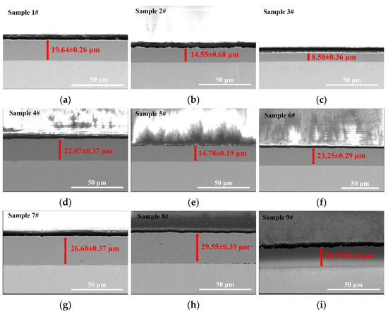
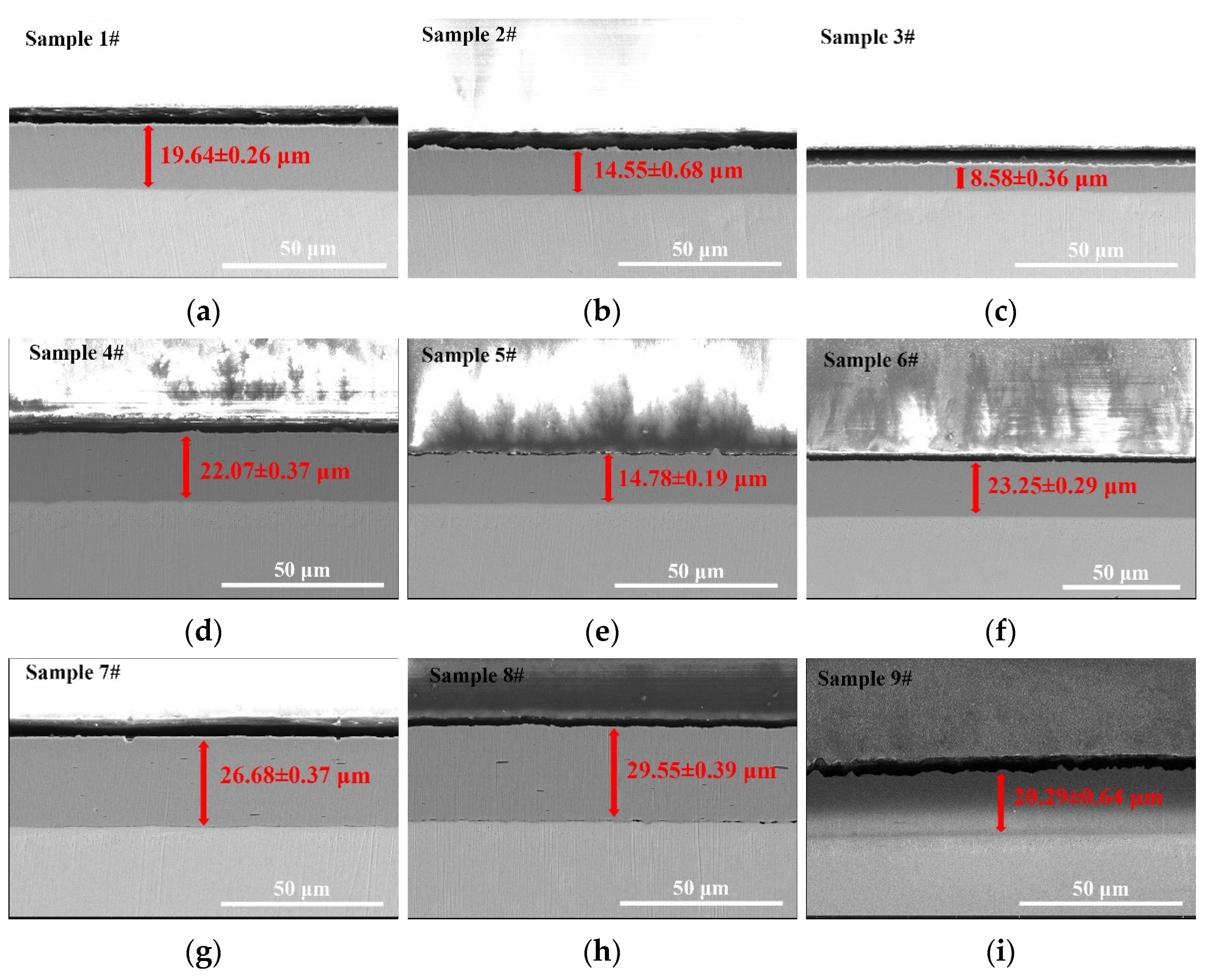
SEM was used to characterize the coating thickness of different Zr-4 alloy samples, with the results presented in Figure 13. As shown in the figure, the coating thickness of all samples ranges approximately from 8 μm to 30 μm. For the coating of each sample, 10 different positions were selected for thickness measurement, and the average value ($\overline{\mathrm{d}}={\displaystyle \frac{\mathrm{I}}{\mathrm{n}}}\sum _{\mathrm{i}=1}^{\mathrm{n}}{\mathrm{d}}_{\mathrm{i}}$) and standard deviation (${\mathsf{\sigma }}_{\mathrm{d}}=\sqrt{{\displaystyle \frac{1}{\mathrm{n}-1}}\sum _{\mathrm{i} = 1}^{\mathrm{n}}{({\mathrm{d}}_{\mathrm{i}}-\overline{ \mathrm{d}})}^2}$) of the actual thickness were calculated. The specific data are listed in Table 3, and these data can be used as the reference thicknesses for this study.

Figure 13. SEM characterization results (reference thickness) of coating for samples: (a) Sample 1#; (b) Sample 2#; (c) Sample 3#; (d) Sample 4#; (e) Sample 5#; (f) Sample 6#; (g) Sample 7#; (h) Sample 8#; (i) Sample 9#.

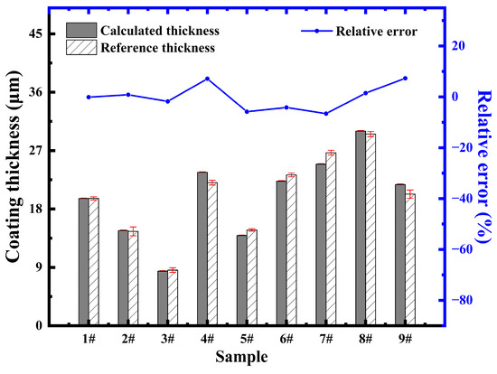
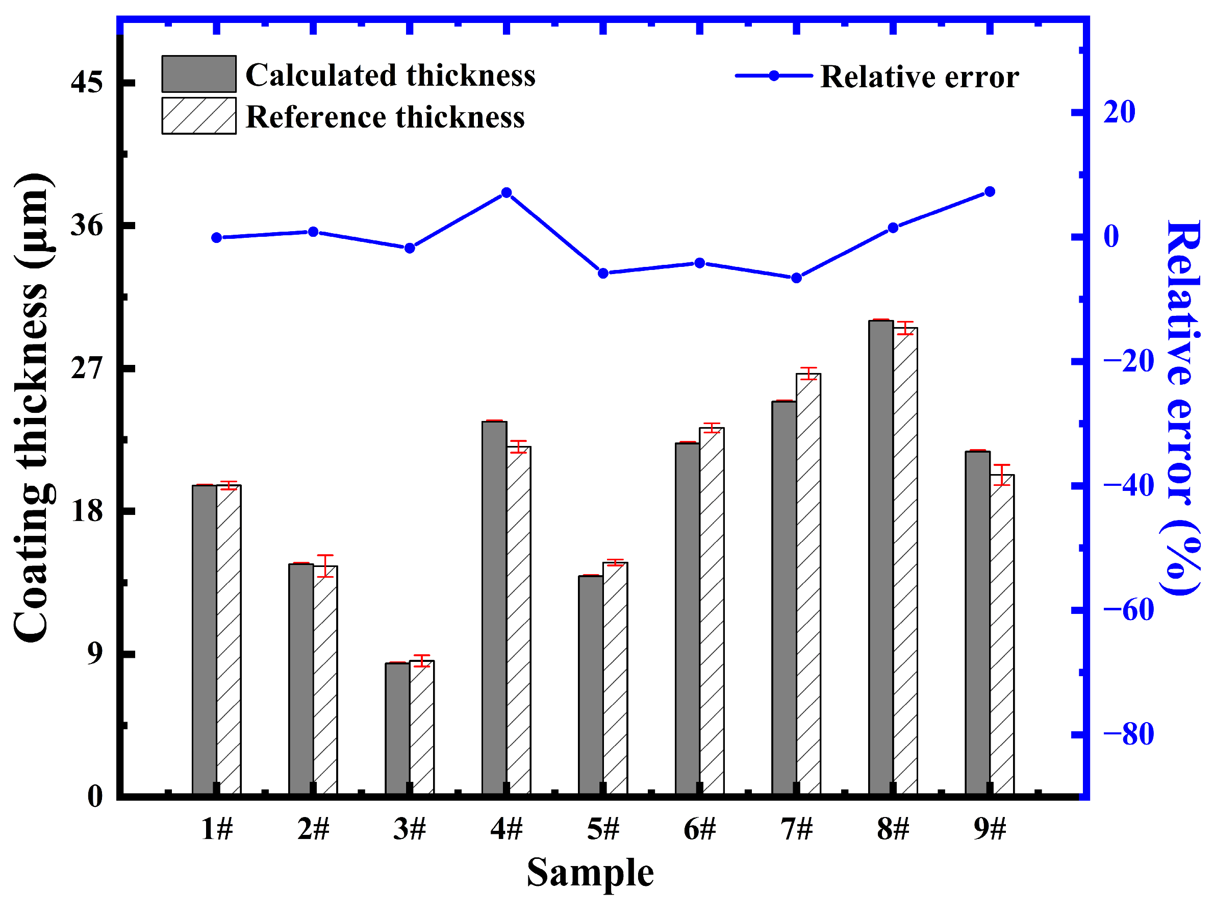
The calculated thicknesses required for the method proposed in this study were obtained by using the FP method of EDXRF. Table 4 and Figure 14 present presents the calculated thicknesses, reference thicknesses, and relative errors of the coatings for samples 1–9#. The calculation of the standard deviation of the calculated thickness values is relatively complex. The parameter $\mathrm{x}={\displaystyle \frac{\mathrm{RI}-{\mathrm{u}}_{\mathrm{RI}}}{{\mathsf{\sigma }}_{\mathrm{RI}}}}$ follows a standard normal distribution $\mathrm{N}\left(0,1\right)$. Then, multiple random samplings are performed on the fluorescence relative intensity $\mathrm{RI}$, as shown in Equations (22) and (23). In the formulas, ${\mathrm{u}}_{\mathrm{RI}} = {\displaystyle \frac{\overline{\mathrm{I}}}{\overline{{\mathrm{I}}_{\mathrm{d}\to \infty }}}}$ can be regarded as the conventional true value of the measured relative intensity. ${\mathsf{\sigma }}_{\mathrm{RI}} = {\displaystyle \frac{\overline{\mathrm{I}}}{\overline{{\mathrm{I}}_{\mathrm{d}\to \infty }}}}\sqrt{{\displaystyle \frac{1}{\mathrm{k}\overline{\mathrm{I}}}} + {\displaystyle \frac{1}{{\mathrm{k}\overline{\mathrm{I}}}_{\mathrm{d}\to \infty }}}}$ is the deviation of the relative intensity. $\mathrm{y}$ is a random number sampled from the range (0,1). Finally, the sampled $\mathrm{RI}$ is substituted into the fundamental parameter method and iterated multiple times to obtain the coating thickness corresponding to the sampling result. Combined with the standard deviation calculation formula, the deviation of the calculated coating thickness for each sample can be obtained.

$$\mathrm{y}=\mathrm{F}\left(\mathrm{x}\right)={\int }_{-\infty }^{\mathrm{x}}{\displaystyle \frac{1}{\sqrt{2\pi }}}{\mathrm{e}}^{{\displaystyle \frac{-{\mathrm{t}}^2}{2}}}\mathrm{dt}\in \left(0,1\right)$$

(21)

$$\mathrm{RI}={\mathrm{u}}_{\mathrm{RI}}+{\mathsf{\sigma }}_{\mathrm{RI}}{\mathrm{F}\left(\mathrm{y}\right)}^{-1}$$

(22)

Table 4. Calculated thickness, reference thickness, and relative error of coatings for samples 1–9#.

Sample	Calculated Thickness (μm)	Reference Thickness (μm)	Relative Error (%)
1#	19.62 ± 0.07	19.64 ± 0.26	−0.10
2#	14.67 ± 0.07	14.55 ± 0.68	0.84
3#	8.43 ± 0.06	8.58 ± 0.36	−1.77
4#	23.64 ± 0.08	22.07 ± 0.37	7.13
5#	13.92 ± 0.07	14.78 ± 0.19	−5.81
6#	22.28 ± 0.08	23.25 ± 0.29	−4.18
7#	24.92 ± 0.08	26.68 ± 0.37	−6.58
8#	30.00 ± 0.09	29.55 ± 0.39	1.50
9#	21.78 ± 0.08	20.29 ± 0.64	7.33

Figure 14. Column charts showing reference thickness and calculated thickness of coatings for samples 1#–9#, along with the corresponding relative error (blue line). The red error bars represent the uncertainties of the calculated thickness and the reference thickness, respectively.

The comparison between the FP-EDXRF calculation results and the SEM measurement results is presented in Table 4. The errors in these results arise from two primary sources. First, the non-uniform thickness caused by the AIP process [33,34]: restricted by coating preparation techniques such as spraying, coating, and curing, thickness variations are inevitable on the flat coating surface. However, the XRF calculation assumes an average thickness over the measured area (ideally a uniform thin layer). Second, statistical fluctuations in detector counts [35]: the interactions of X-rays with matter (photoelectric effect, Compton scattering, Rayleigh scattering) exhibit randomness. Consequently, the full-energy peak counts display statistical variability. Averaging multiple measurement results can significantly reduce errors caused by these statistical fluctuations.

Comparing the two sets of data, it is found that the relative errors for Samples 4#, 5#, 7#, and 9# are larger (with a maximum value of 7.33%), possibly attributed to the non-uniformity of the coating. Samples 1#, 2#, 3#, 6#, and 8# show good agreement between calculated thickness values and reference thickness values (with relative errors less than ±5%), indicating that the FP-EDXRF technique can rapidly and accurately characterize the thickness of Cr coatings on Zr alloys.

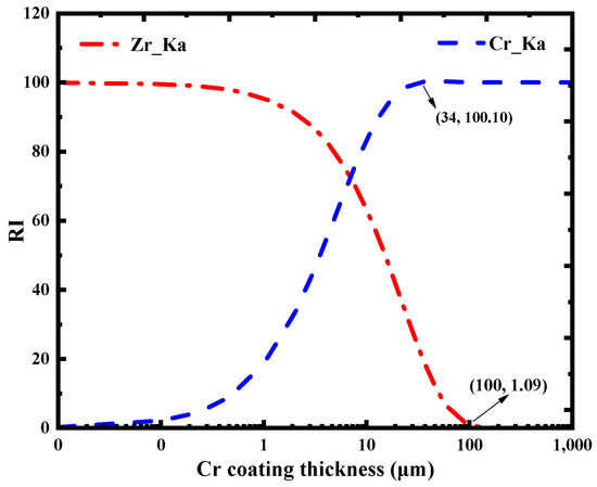
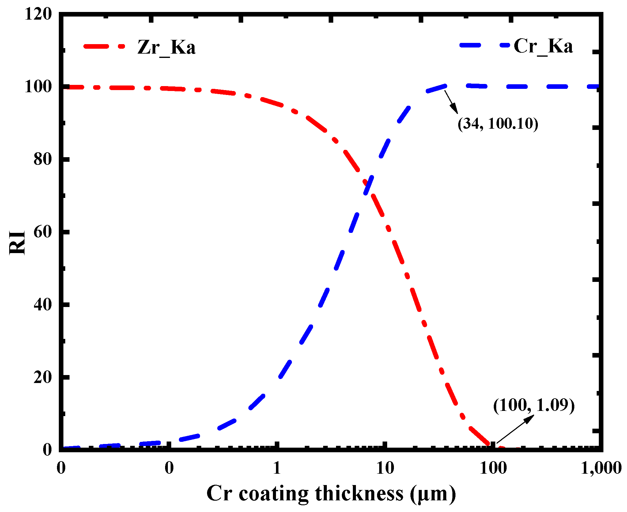
On the other hand, the theoretical RI of Zr K_α and Cr K_α rays as a function of Cr coating thickness is shown in Figure 15. It can be observed that the initial RI of Zr K_α rays is close to 100% and decreases gradually with the increase in Cr coating thickness, and when the thickness reaches approximately 100 μm, the RI approaches 1.09 and tends to stabilize. In contrast, the initial RI of Cr K_α rays is close to 0 and increases rapidly as the Cr coating thickness rises, and when the thickness is around 34 μm, the RI approaches 100 and reaches saturation. Accordingly, when Zr is used as the target element, the maximum measurable coating thickness can reach 100 μm. When Cr serves as the target element, the maximum measurable coating thickness is limited to 34 μm. This is attributed to the fact that Cr exhibits a larger mass absorption coefficient than Zr. When the coating thickness exceeds 34 μm, the RI becomes nearly constant, making it impossible to characterize samples with thicker coatings using Cr K_α rays.

Figure 15. Relative intensity (RI) of Zr_K_α and Cr_K_α as a function of Cr coating thickness (nm). The abscissa is presented on a ‘Log10’ scale.

5. Conclusions

In this work, FP-EDXRF was successfully applied to the thickness measurement of Zr alloy coatings. Compared with conventional techniques such as cross-sectional SEM and metallographic methods, this method offers significant advantages including non-destructive analysis, high efficiency, and freedom from elaborate sample preparation. Validation experiments on nine Zr alloy specimens with different coating thicknesses showed that the maximum relative error was 7.33%, while most samples presented relative errors within ±5%. The observed deviations mainly originate from two sources: one is the thickness inhomogeneity introduced during the AIP process, and the other is the statistical fluctuations of detector counts. These results verify the reliability, stability, and accuracy of the FP-EDXRF method for Zr alloy coating thickness characterization. This approach provides a valuable tool for material quality control and structural integrity evaluation in nuclear applications.

References

- Zuo, D.; Du, P.N.; Luo, W.; Chen, H.; Wang, Y.; Wei, T.G.; Zhang, R.Q.; Liu, H.Q. Effect of Cr coating on creep behavior of zircaloy-4 alloy. Trans. Nonferrous Met. Soc. China 2024, 34, 1533. [Google Scholar] [CrossRef] [Scilit]
- Wei, T.G.; Zhang, R.Q.; Yang, H.Y.; Liu, H.; Qiu, S.Y.; Wang, Y.; Du, P.N.; He, K.; Hu, X.G.; Dong, C. Microstructure, corrosion resistance and oxidation behavior of Cr-coatings on Zircaloy -4 prepared by vacuum arc plasma deposition. Corros. Sci. 2019, 158, 108077.1. [Google Scholar] [CrossRef] [Scilit]
- Kuprin, A.S.; Belous, V.A.; Voyevodin, V.N.; Vasilenko, R.L.; Ovcharenko, V.D.; Tolstolutskaya, G.D.; Kopanets, I.E.; Kolodiy, I.V. Irradiation resistance of vacuum arc chromium coatings for zirconium alloy fuel claddings. J. Nucl. Mater. 2018, 510, 163. [Google Scholar] [CrossRef] [Scilit]
- Brachot, J.C.; Rouesne, E.; Ribis, J.; Guilbert, T.; Urvoy, S.; Nony, G.; Toffolon-Masclef, C.; Le Saux, M.; Chaabane, N.; Palancher, H.; et al. High temperature steam oxidation of chromium-coated zirconium-based alloys: Kinetics and process. Corros. Sci. 2020, 167, 108537. [Google Scholar] [CrossRef] [Scilit]
- Li, Q.; Song, P.; Zhang, R.Q.; Li, Z.H.; Wang, Y.; Du, P.N.; Lu, J.S. Oxidation behavior and Cr-Zr diffusion of Cr coatings prepared by atmospheric plasma spraying on zircaloy—4 cladding in steam at 1300 °C. Corros. Sci. 2022, 203, 110378. [Google Scholar] [CrossRef] [Scilit]
- Wang, S.X.; Bai, S.X.; Zhu, L.A.; Ye, Y.C.; Wang, Z.; Li, S.; Tang, Y. Research progress of chromium coating on zirconium alloy for nuclear fuel cladding. Surf. Technol. 2021, 50, 221. [Google Scholar] [CrossRef] [Scilit]
- Wu, S.H.; Wang, D.; Zhang, Y.P.; Wu, X.C.; Tian, W.X.; Qiu, S.Z.; Su, G.H. Performance evaluation of accident tolerant Cr-coated Zr alloy cladding under accident conditions based on a refined degradation model. Prog. Nucl. Energy 2024, 176, 105359. [Google Scholar] [CrossRef] [Scilit]
- Ling, H.J.; Sun, S.L.; Jiao, Y.G.; Shen, Z.W. Application of laser diameter measurement and ultrasonic thickness gauging in the measurement of zirconium alloy pipe. Nondestruct. Test. Technol. 2018, 4, 50. [Google Scholar] [CrossRef]
- Shibata, T.; Ishihara, M. Ultrasonic signal characteristics by pulse-echo technique and mechanical strength of graphite materials with porous structure. Nucl. Eng. Des. 2001, 203, 133. [Google Scholar] [CrossRef] [Scilit]
- Zou, L.; Li, H.; Wang, W.X.; Huang, Y.; Li, Y.T. A precision grinding technology for zirconium alloy tubes based on ultrasonic wall thickness automatic measurement system. Int. J. Adv. Manuf. Technol. 2022, 121, 323. [Google Scholar] [CrossRef] [Scilit]
- Ren, J.B.; Tang, Y.M.; Xu, G.P.; Wang, X.Q.; Cai, Y.K. Research of Scanning Acoustic Microscope Thickness Measurement Method for Zirconium Alloy Multilayered Composite Material. Nucl. Power Eng. 2016, 37, 44. [Google Scholar] [CrossRef]
- Alig, I.; Tadjbach, S.; Krüger, P.; Oehler, H.; Lellinger, D. Characterization of coating systems by scanning acoustic microscopy: Debonding, blistering and surface topology. Prog. Org. Coat. 2009, 64, 112. [Google Scholar] [CrossRef] [Scilit]
- Oehler, H.; Alig, I.; Lellinger, D.; Bargmann, M. Failure modes in organic coatings studied by scanning acoustic microscopy. Prog. Org. Coat. 2012, 74, 719. [Google Scholar] [CrossRef] [Scilit]
- Liu, Y.S.; Ge, H.H.; Suo, W.Y.; Ma, X.D.; Deng, Z.Y.; Gao, S.J.; Li, H.Y. Simulation optimization and design of eddy current detection probe for the oxidation film thickness of zirconium alloy shell. Nondestruct. Test. 2025, 47, 40. [Google Scholar] [CrossRef]
- Li, Y.; Xiao, Q.; Peng, L.; Huang, S.; Ye, C. A precise oxide film thickness measurement method based on swept frequency and transmission cable impedance correction. Sensors 2025, 25, 579. [Google Scholar] [CrossRef] [Scilit]
- Yusa, N.; Janousek, L.; Rebican, M.; Chen, Z.; Miya, K.; Chigusa, N.; Ito, H. Detection of embedded fatigue cracks in inconel weld overlay and the evaluation of the minimum thickness of the weld overlay using eddy current testing. Nucl. Eng. Des. 2006, 18, 1852. [Google Scholar] [CrossRef] [Scilit]
- Zhou, G.Z.; Zhang, N.; Liang, J.; Xu, X.B.; Tao, Y. Study of multi-parameters separation for oxide film thickness measurement. In Proceedings of the 2023 IEEE Far East NDT New Technology & Application Forum (FENDT), Tianjin, China, 13–15 June 2023; IEEE: New York, NY, USA, 2023. [Google Scholar] [CrossRef] [Scilit]
- Sethuraman, A.; Rose, J.H. Rapid inversion of eddy current data for conductivity and thickness of metal coatings. J. Nondestruct. Eval. 1995, 14, 40. [Google Scholar] [CrossRef] [Scilit]
- Jeong, Y.N.; Nwabu Okwuosa, C.; Hwang, J.W.; Hur, J.W. Optimization of flow rate for uniform zinc phosphate coating on steel cylinders: A study on coating uniformity and elemental composition using scanning electron microscopy (SEM). Materials 2025, 18, 2442. [Google Scholar] [CrossRef] [Scilit]
- Hou, C.; Sun, J.; Kashkarov, E.B.; Wang, J.Y.; Lin, Z.; Sun, F.; Ma, H.L. Multi-response optimization of arc ion plated cr coating on zr alloy claddings based on taguchi method and grey relational theory. J. Nucl. Mater. 2026, 625, 156533. [Google Scholar] [CrossRef] [Scilit]
- Ren, X.D.; Ruan, L.; Yuan, S.Q.; Yang, H.M.; Zhan, Q.B.; Zheng, L.M.; Wang, Y.; Dai, F.Z. Metallographic structure evolution of 6061-t651 aluminum alloy processed by laser shock peening: Effect of tempering at the elevated temperatures. Surf. Coat. Technol. 2013, 221, 111. [Google Scholar] [CrossRef] [Scilit]
- Liu, Z.H.; Dai, Y.K. Measurement for copper layer thickness and coating thickness of bimetallic wire by metallographic microscope. Electr. Wire Cable 2014, 6, 8. [Google Scholar] [CrossRef]
- Biswas, S.; Rupawate, V.H.; Hareendran, K.N.; Roy, S.B. A novel method for the determination of zirconium in uranium-zirconium alloy fuel using Energy-dispersive X-ray Fluorescence (EDXRF) technique. In Fourth International Symposium on Nuclear Analytical Chemistry (NAC-4); Bhabha Atomic Research Centre: Mumbai, India, 2010. [Google Scholar]
- Beckhoff, B.; Kannigießer, H.B.; Langhoff, N. Handbook of Practical X-Ray Fluorescence Analysis; Springer: Berlin/Heidelberg, Germany, 2006; pp. 369–370. Available online: https://link.springer.com/content/pdf/bfm:978-3-540-36722-2/1.pdf (accessed on 6 February 2026).
- Liu, Y.L.; Zhang, Q.X.; Zhang, J.; Bai, H.T.; Ge, L.Q. Quantitative energy-dispersive X-ray fluorescence analysis for unknown samples using full-spectrum least-squares regression. Nucl. Sci. Tech. 2019, 30, 11. [Google Scholar] [CrossRef] [Scilit]
- Sherman, J. The theoretical derivation of fluorescent x-ray intensities from mixtures. Spectrochim. Acta 1955, 7, 283. [Google Scholar] [CrossRef] [Scilit]
- Shiraiwa, T.; Fujino, N. Theoretical calculation of fluorescent x-ray intensities in fluorescent x-ray spectrochemical analysis. Jpn. J. Appl. Phys. 1966, 5, 886. [Google Scholar] [CrossRef] [Scilit]
- Revenko, A.G.; Tsvetyansky, A.L.; Eritenko, A.N. X-ray fluorescence analysis of solid-state films, layers, and coatings. Radiat. Phys. Chem. 2022, 197, 110157. [Google Scholar] [CrossRef] [Scilit]
- Sui, S.S.; Wei, J. Calculation of multilayer film thickness using fundamental parameter method of XRF. J. Univ. Electron. Sci. Technol. China 1995, 24, 67. [Google Scholar]
- Pavlinsky, G.V.; Dukhanin, A.Y.; Baranov, E.O.; Portnoy, A.Y. Theory of the implementation of the fundamental parameter method for the X-ray fluorescence determination of low-atomic-number elements. J. Anal. Chem. 2006, 61, 654. [Google Scholar] [CrossRef] [Scilit]
- Birks, L.S.; Gilfrich, J.V.; Criss, J.W. NRLXRF, a Fortran Program for X-Ray Fluorescence Analysis: Users’ Guide; N.R. Laboratory: Washington, DC, USA, 1977. Available online: https://www.nist.gov/system/files/documents/mml/csd/inorganic/user_guide.pdf (accessed on 6 February 2026).
- Zhang, Q.X.; Li, H.; Xiao, H.F.; Zhang, J.; Li, X.Z.; Yang, R. An improved PD-AsLS method for baseline estimation in EDXRF analysis. Anal. Methods 2021, 13, 2037. [Google Scholar] [CrossRef] [Scilit]
- Fuchs, H.; Engers, B.; Hettkamp, E.; Mecke, H.; Schultz, J. Deposition rate and thickness uniformity of thin films deposited by a pulsed cathodic arc process. Surf. Coat. Technol. 2001, 142–144, 655. [Google Scholar] [CrossRef] [Scilit]
- Zhao, Y.H.; Guo, C.Q.; Yang, W.J.; Chen, Y.Q.; Yu, B.H. TiN films deposition inside stainless-steel tubes using magnetic field-enhanced arc ion plating. Vacuum 2015, 112, 46. [Google Scholar] [CrossRef] [Scilit]
- Chantler, C.T.; Creagh, D.C. X-ray interactions with matter. Int. Tables Crystallogr. 2024, 1, 21. [Google Scholar] [CrossRef] [Scilit]
Disclaimer/Publisher’s Note: The statements, opinions and data contained in all publications are solely those of the individual author(s) and contributor(s) and not of MDPI and/or the editor(s). MDPI and/or the editor(s) disclaim responsibility for any injury to people or property resulting from any ideas, methods, instructions or products referred to in the content. |
© 2026 by the authors. Licensee MDPI, Basel, Switzerland. This article is an open access article distributed under the terms and conditions of the Creative Commons Attribution (CC BY) license.