


Abstract
Cavitation flow within airless spray nozzles critically influences both atomization quality and nozzle longevity. However, its highly transient and multiphase-coupled nature poses significant challenges to the predictive accuracy of turbulence models. To improve numerical simulation fidelity, this study develops an improved dynamic Wall-Adapting Local Eddy-viscosity (WALE) subgrid-scale model for Large Eddy Simulation (LES). Building on the standard WALE formulation, the model incorporates a dynamic coefficient determined via the Germano identity and a least-squares approach, which enables it to adaptively capture the turbulence modulation effects induced by cavitation. Coupled with a Volume of Fluid (VOF) multiphase flow method, this framework is employed to systematically simulate the complex internal nozzle flow under varying spray pressures, coating viscosities, and surface tensions. Results indicate that the improved dynamic WALE model increases numerical stability by approximately 15% compared with the standard model. The internal flow can be partitioned into three regions: a potential-flow acceleration region, a cavitation-induced fluctuation region, and an outlet formation region. Within the cavitation-induced fluctuation region near the wall, cavitation generates a local double-peaked velocity profile and pronounced pressure pulsations. Cavitation intensity increases approximately linearly with spray pressure but decreases with increasing viscosity and surface tension. Both the discharge coefficient and velocity coefficient decrease linearly with increasing cavitation number, indicating that moderate cavitation can enhance instantaneous throughput by altering the flow-field structure. Finally, outflow mass-flow experiments validate the numerical model’s reliability: the improved dynamic WALE model achieves prediction errors ranging from 0.47% to 11.91%, substantially outperforming the standard WALE model, which has errors ranging from 1.27% to 21.10%.
1. Introduction
Airless spray technology, as an efficient and environmentally friendly coating process, is widely applied in anticorrosion projects for large structures [1] such as ships, bridges, and storage tanks. The internal flow characteristics of its core component—the nozzle—directly determine the quality of paint atomization and spraying efficiency. Flow within the nozzle is typically accompanied by high velocity, intense shear, multiphase interactions, and cavitation. The occurrence of cavitation, in particular, not only affects flow stability but can also induce nozzle wear and nonuniform atomization [2]. Therefore, an in-depth investigation of the internal flow mechanisms in airless spray nozzles, especially the interaction between cavitation and turbulence, is of great significance for optimizing nozzle design and improving spray quality.
The choice of turbulence model exerts a decisive influence on the accuracy of cavitating flow simulations. Direct numerical simulation (DNS) [3] can resolve vortical structures across all scales with high fidelity, but its computational cost is prohibitive for engineering applications. Reynolds-averaged methods (RANS) [4] treat turbulence through temporal averaging and are computationally efficient, yet they tend to smear transient details inherent to the cavitation process. In contrast, LES [5], which directly resolves large-scale vortices while modeling the subgrid scales, can capture the dynamic evolution of cavitation phase interfaces more effectively at a controllable computational cost.
In LES, subgrid-scale (SGS) models [6] are critical to simulation accuracy. The classical Smagorinsky model assumes eddy viscosity proportional to the magnitude of the strain rate, but it performs poorly in near-wall regions and in non-equilibrium flows. The WALE (Wall-Adapting Local Eddy-viscosity) model proposed by Nicoud and Ducros [7] introduces a mixed tensor of strain-rate and rotation-rate, yielding a natural decay of eddy viscosity near walls and making it better suited to wall-bounded turbulence and shear flows; however, its tendency to over-dissipate remains pronounced in high-Reynolds-number flows and in strongly vortical systems [8,9]. Moreover, the standard WALE model employs a constant model coefficient and does not account for the influence of dynamic processes such as phase change and cavitation on turbulent energy transport. To address this, researchers have proposed determining model coefficients dynamically using the Germano identity [10] and Lilly’s least-squares procedure, thereby allowing the coefficients to adapt to non-equilibrium flows. Building on this approach, the present work proposes an improved dynamic WALE model that introduces a test-filter scale and dynamic coefficient adjustment to more accurately represent turbulence modulation during cavitation, thereby enhancing the model’s applicability to gas–liquid two-phase flows. Nonetheless, this method theoretically requires averaging the model coefficient under the assumption of flow homogeneity; this averaging lacks a clear physical justification, the secondary filtering significantly reduces computational efficiency, errors can arise near irregular boundaries, and the solution of vortical fields still exhibits over-dissipative behavior [11,12]. To overcome over-dissipation, Hughes et al. [13] proposed the variational multiscale model (VMM) to distinguish large- and small-scale vortical motions. A regularized variant model (RVM) was initially proposed by Jeanmart et al. [14] in an effort to improve vortical-field predictions; subsequently, Bricteux et al. [15] investigated this approach for predicting horizontal wall flows in low-Re channel flows and found it inadequate for accurately capturing the complex asymptotic near-wall behavior. In recent years, methods employing dynamic model coefficients have attracted considerable attention as remedies for over-dissipation. Examples include the explicit algebraic subgrid-scale scale-similarity model of Montecchia et al. [16], the Lagrangian dynamic model (LDM) of Tellez-Álvarez et al. [17], and the dynamic k-equation subgrid models of Shukla et al. [18] and Sircar et al. [19]; these models enhance computational accuracy by introducing dynamic evolution equations and explicit filtering operations.
Early research on cavitating flows focused on hydrodynamics, emphasizing propellers and hydrofoils. Recently, advances in spraying and fuel injection have made nozzle cavitation a major focus. Most studies focus on fuel injection systems, while systematic studies of cavitating flow in airless-spraying nozzles remain scarce. Internal flow in these nozzles shows strong transients, high shear, and multiphase coupling. Mechanisms of cavitation evolution and interactions with turbulence are not yet clearly understood. Current turbulence models cannot accurately describe these processes.
Therefore, this study is based on the fundamental framework of LES. It uses the Germano identity, a mathematical equation that relates sub-grid-scale stresses, a least-squares procedure for model optimization, and a dynamic coefficient model that adapts model parameters during simulations. These steps markedly enhance the applicability and accuracy of the WALE model for transient gas–liquid two-phase flows. The improved dynamic WALE model offers significant advantages in predicting cavitating flows, which involve the formation and collapse of vapor bubbles in a liquid. It more accurately captures interactions between cavitation and turbulence, or chaotic fluid motion. The model provides theoretical support and numerical tools for optimizing the design of airless spray nozzles. It also offers a transferable modeling approach for other strongly transient multiphase flow problems.
2. Numerical Model
2.1. Turbulence Model
The internal flow within airless spray nozzles is unsteady. Thus, the choice of turbulence model must balance computational accuracy and cost. Large Eddy Simulation (LES), by directly resolving large-scale vortices and modeling the small-scale ones, can accurately capture cavitation interfaces at controllable computational expense. Its suitability for investigating cavitating flows inside nozzles has been confirmed by relevant studies [20,21].
LES decomposes flow field variables using a filtering operation, which mathematically separates them into resolvable large scales (motions that can be directly calculated) and unresolvable small scales (motions too fine to be represented in the simulation). Vortical structures—coherent rotations in the flow—larger than the cutoff scale set by the filter are treated as large-scale, and their governing equations are solved directly:
where and denote the unknown velocity (m/s) and pressure (Pa) of the large-scale vortices; and denote spatial coordinate components (m); t denotes time (s); ρ represents the fluid density (kg/m3); denotes the sub-grid scale stress tensor (Pa); ν denotes the kinematic viscosity of the fluid (m2/s).
In the expression, in addition to the unknowns and representing large-scale vortices, a subgrid-scale stress arising from small-scale vortex motion also appears. Based on the Boussinesq hypothesis [22], this turbulent stress can be modeled as:
where is the trace of the subgrid stress tensor (Pa), representing the kinetic energy carried by unresolved small-scale eddies; in incompressible flows it can be incorporated into a modified pressure term; denotes kronecker delta (Dimensionless); denotes the sub-grid scale eddy viscosity coefficient (Pa·s); denotes the resolved-scale strain-rate tensor (s−1), defined as:
where denotes the subgrid-scale viscosity. In the WALE model it should depend not only on the strain rate but also on the rotational effects of the fluid, and it should decay gradually near the wall; this is achieved by introducing a mixed tensor (dimensionless):
In the equation, denotes the filtered velocity gradient tensor (s−1), denotes the square of the velocity gradient tensor (s−2), and denotes its trace (s−2). Based on this, the subgrid-scale viscosity can be defined as:
where is a model constant (taken as 0.325 in the non-aerated spray atomization case, dimensionless); is the filter scale (m), taken as the cubic root of the grid-cell volume; denotes the intermediate variable defined in the formula (s−1).
The standard WALE model is constructed with a constant model coefficient and is applicable to single-phase incompressible flows, but it does not account for the influence of phase change on turbulent energy transport; therefore, it cannot accommodate local turbulence variations induced by strong shear, phase change, and cavitation. To account for these dynamic effects, a test filter scale larger than the grid filter scale Δ is introduced, and the model coefficient is determined from the resolved scales using the Germano identity. Specifically, the Germano identity can be written as:
Here, denotes the Leonard stress (Pa), computed from the solvable-scale velocity field and representing the turbulence fluctuations resolvable at the test filter scale. represents the grid-scale subgrid stress (Pa), and represents the test-scale subgrid stress (Pa).
Under the Boussinesq hypothesis, only the deviatoric part of the stress is required; therefore, the deviatoric part of an arbitrary second-order tensor is defined as follows:
where is an arbitrary second-order tensor (Pa); denotes the trace of (Pa); is the Kronecker delta (dimensionless); denotes the deviatoric (trace-free) part of (Pa).
Taking the traceless part of Equation (6) yields:
where denotes the deviatoric part of the Leonard stress tensor (Pa); denotes the deviatoric part of the test-scale subgrid stress tensor (Pa); denotes the deviatoric part of the filtered grid-scale subgrid stress tensor (Pa).
Since the Boussinesq eddy-viscosity assumption is applied to the deviatoric part of the SGS stress, the dynamic procedure is constructed in terms of the trace-free (deviatoric) components. At this stage, the stress expressions at the filter scale and at the test-filter scale can be obtained:
where denotes the sub-grid-scale eddy viscosity coefficient under the test scale (Pa·s); denotes test the density after filtering (kg/m3); denotes the scalar function of the WALE model (s−1); denotes the resolved-scale strain-rate tensor at the grid-filter level (s−1); denotes the deviatoric part of the subgrid-scale stress tensor at the grid-filter level (Pa); denotes the subgrid-scale stress tensor (Pa); denotes the trace of (Pa); denotes the deviatoric part of the subgrid-scale stress tensor at the test-filter level (Pa); denotes the subgrid-scale stress tensor at the test-filter level (Pa); denotes the trace of (Pa); denotes the resolved-scale strain-rate tensor at the test-filter level (s−1); Δ is the grid-filter scale (m); is the WALE model constant (dimensionless); denotes the scalar function of the WALE model under the test scale (s−1).
Substituting Equation (9) into the Germano identity (6):
where denotes the Leonard stress tensor (Pa); denotes the trace of (Pa); denotes an intermediate tensor of the defined dynamic model (Pa).
Equation (10) is a tensor equation involving six independent components, but with only one unknown ; it therefore constitutes an overdetermined system, necessitating the definition of an error tensor (Pa):
Using the least squares method [23] to determine the optimal solution for , the mean square of the second-order error is taken as the objective function in the statistical sense.
where denotes the mean squared magnitude of the deviatoric Leonard stress (Pa2); denotes the mean correlation between and (Pa2); denotes the mean squared magnitude of the tensor (Pa2); J denotes the objective function to be minimized, representing the total mean-squared error between the modeled and resolved stresses (Pa2); denotes the average operator (dimensionless).
It is worth noting that the averaging operator in Equation (12) represents a local statistical averaging used to approximate the ensemble average required by the dynamic procedure. This operation is not heuristic smoothing; it is introduced to obtain a converged estimate of the second-order correlations and under the assumption that varies slowly within the support of the test filter. To maintain locality in strongly heterogeneous nozzle flows, is evaluated using a localized spatial kernel, rather than a global spatial average.
We differentiate with respect to and set it to the stationary value; since the averaging operator is independent of and linear, differentiation and averaging commute:
Therefore we obtain:
Since is a traceless tensor , then
Substituting the above expression back into Equation (14) yields:
In dynamic models, is essentially a statistic determined by second-order correlations. Strictly speaking, the above least-squares procedure should be based on ensemble averaging in order to obtain convergent values of and . Ensemble averaging cannot be performed in a single LES realization, so a local spatial average is used to approximate the ensemble average (quasi-ergodic/local ergodicity assumption), that is:
where denotes the local spatial average of a field variable ϕ, approximating the ensemble average in a single LES realization; denotes a generic field variable (e.g., velocity, stress component) as a function of position r and time t (units depend on the variable); denotes the volume of the local averaging region (m3); denotes the local neighborhood centered at x (the scale is typically taken on the order of O(Δ∼2Δ)), used to obtain statistical convergence of the relevant quantities and to suppress noise amplification when is small; r denotes the position vector (m).
Because local strongly non-uniform regions may exhibit instantaneous negative or excessively large values, and in order to avoid excessively strong counter-dissipation and to ensure the realizability of the SGS viscosity and numerical stability, is clamped to yield the following expression:
In summary, the sublattice viscosity can be expressed as:
2.2. Two-Phase Flow Model
The tracking of the gas–liquid interface in the gasless spray process is accomplished by solving the conservative volume fraction transport equation; its mathematical essence is the discrete solution of the phase-fraction continuity equation within the Eulerian framework. The volume-fraction continuity equations for the two phases can be expressed as:
where and denote the volume fractions of the gas phase and the liquid phase; and denote the densities (kg/m3) of the air phase and the coating phase, respectively; and denote their velocity vectors (m/s), respectively; and are the mass source terms (kg/m3·s); and represent the mass transfer (kg/m3·s) between the coating phase and the air phase, respectively.
Within the nozzle, heat and mass transfer processes can be neglected [24]; therefore, it is only necessary to formulate the continuity and momentum equations for the air phase and the coating (liquid) phase:
where μ denotes the dynamic viscosity of the air phase or the coating phase (N·s/m2); represents the local gravitational acceleration vector (m/s2); p denotes the pressure (Pa); denotes the gradient operator; denotes the velocity vector (m2/s2); represents other body forces, including surface tension (N); u and v denote the velocity vector (m/s). In the continuity equation, it is denoted as u, while in the momentum equation, it is denoted as v. However, their physical meanings are the same.
During the spraying process, the coating is driven at high speed through a nozzle with a very small aperture by an extremely large pressure differential. To rigorously justify the exclusion of the gravity term in the momentum equation, a dimensionless analysis using the Froude number Fr is performed. The Froude number, which represents the ratio of inertial forces to gravitational forces, is defined as:
where U denotes the characteristic flow velocity (m/s); g denotes the gravitational acceleration (m/s2); L denotes the characteristic length scale (m). Under the operating conditions of this study, the spray pressure typically ranges from 10 to 20 MPa. Estimating based on Bernoulli’s principle, the characteristic velocity inside and at the outlet of the nozzle can exceed 140 m/s. Taking the characteristic length as the nozzle outlet diameter of 0.71 mm, and noting that the diameters of atomized coating particles do not exceed the nozzle diameter, substitution into the calculation yields:
Because the computed , this indicates that, within the high-speed flow region inside the nozzle, inertial effects overwhelmingly dominate, and gravity has a negligible influence on the flow structure and the trajectories of large droplets. Therefore, the gravity term in the momentum Equation (21) can be omitted to improve computational efficiency.
2.3. Cavitation Model
During the internal flow of a gasless spray nozzle, the high-pressure coating flowing through narrow passages can experience a sudden local pressure drop to below the saturation vapor pressure, leading to cavitation. To compute the net phase-change rate under cavitation effects, Schnerr and Sauer [25] adopted a multiphase flow cavitation modeling approach and proposed the following two-phase continuity equations:
where denotes the volumetric fraction of the vapor phase; ρv, ρl, and ρ denote the densities of the vapor phase, the coating phase, and the mixture phase (kg/m3), respectively; denotes the relative velocity (m/s); Rv and Rl denote the mass transfer source terms (kg/(m3·s)) associated with vapor bubble growth and collapse, respectively, i.e., the net phase change rate. The mixture density ρm is defined as:
Combining Equation (24) can yield the relationship between the mixture-phase density and the vapor-phase volume fraction:
where the gas-phase volume fraction can be calculated from the bubble number density n (m−3(1/m3)) and the bubble radius (m):
By combining the above equations, one obtains an expression for the net phase-change rate R:
In the equation, and denote the empirical calibration coefficients (dimensionless) for evaporation and condensation, respectively, typically taking values of 1 and 0.2; P and Pv denote the mixed-phase pressure and the saturated vapor pressure (Pa).
3. Numerical Simulation Setup
3.1. Computational Domain and Meshing
The internal flow domain of the nozzle was constructed using SpaceClaim, as shown in Figure 1. The geometric model shows the flow path from inlet to outlet. The wall indicated by the left blue arrow denotes the flow inlet. The V-groove wall indicated by the red arrow to the right represents the outlet structure. Relevant geometric parameters are listed in Table 1.
Figure 1.
Computational domain of the flow region inside the nozzle.
Table 1.
Computational domain size of the flow area inside the nozzle.
The computational domain was discretized using the Poly-Hexcore hybrid meshing strategy provided by FluentMeshing. This strategy accounts for differences in flow characteristics across regions and applies region-specific mesh treatments. In near-wall regions, where geometric curvature varies and flow gradients are large, polyhedral elements are used for local refinement. This effectively resolves near-wall flow details. In the central axial flow region, where flow is relatively stable and fully developed, hexahedral elements are used for a coarser discretization. This balances computational efficiency and numerical accuracy.
Key mesh parameters were set as follows: the near-wall region comprises four buffer layers and three peel layers, with the mesh growth rate limited to 1.2. To mitigate local accuracy loss caused by rapid volumetric expansion during the transition between hexahedral elements and the near-wall region, polyhedral cells were introduced in the transitional zone to effect a smooth change in cell size and a stable transfer of the numerical solution. The final mesh is shown in Figure 2, where the dashed boxed region indicates an enlarged view of the local mesh; its overall quality is good and satisfies the requirements for subsequent high-fidelity flow simulations.
Figure 2.
Mesh generation for the computational domain of the internal flow region of the nozzle.
3.2. Mesh Independence Verification
Grid-independence verification is an essential step in CFD to ensure the reliability and accuracy of numerical predictions. In this study, five mesh resolutions (Table 2) were generated and simulated under identical initial conditions and boundary settings. Because the flow is isothermal and incompressible, the LES framework with the WALE subgrid-scale model was employed, and the coupled pressure–velocity solver was used. Each control volume contains approximately four primary degrees of freedom (DOF), namely three velocity components and pressure; accordingly, the total degrees of freedom considered are approximately in the range [0.5, 2.1] million, corresponding to roughly [120,000, 520,000] cells. Among all nozzle cross-sections, the region near the V-shaped groove adjacent to the nozzle exit exhibits the steepest geometric gradients and the smallest flow area; accordingly, the minimum mesh size was specified at the outlet. The reported mean skewness is used solely to characterize the surface mesh quality in the vicinity of the V-shaped groove, whereas orthogonality serves as an indicator of the overall volumetric mesh quality across the entire nozzle domain.
Table 2.
Mesh parameters.
Figure 3a shows the relationship between mesh size and quality metrics: as the characteristic size increases, the number of elements decreases; the mean mesh quality exhibits a decreasing trend, whereas the minimum inverse orthogonality metric increases. This apparently contradictory phenomenon actually reflects a trade-off between numerical discretization accuracy and geometric approximation. Fine meshes can capture geometric gradients with high fidelity but unavoidably introduce a larger number of low-orthogonality elements; conversely, coarse meshes smooth geometric details while yielding improved element shape and numerical stability. It can also be observed that the mean skewness at the nozzle exit increases progressively as the minimum mesh size is reduced, indicating that stronger mesh refinement in regions with large local geometric gradients exacerbates face-cell distortion. Notably, when the minimum size is reduced further from 0.03 mm to 0.025 mm, the mean skewness exhibits a pronounced jump, implying that mesh generation at this scale becomes more sensitive to geometric features and that local cell shapes are more readily influenced by complex curvature, narrow-slot geometries, and localized transition-refinement strategies. Therefore, when further refining the mesh to improve geometric resolution, concomitant attention must be paid to the resulting changes in local mesh quality at the exit.
Figure 3.
Curves of parameters related to mesh independence verification: (a) Grid quality verification. (b) Verification of import and export quality flow.
Figure 3b shows how inlet and outlet mass flow rates vary with mesh count. As the number of mesh elements increases, these flows gradually converge and stabilize. Beyond a certain mesh density, their fluctuations become negligible, indicating that the numerical solution no longer depends on further mesh refinement.
Considering computational accuracy and efficiency, this chapter adopts a mesh with a minimum cell size of 0.03 mm and 404,960 cells for the subsequent numerical simulation of the nozzle’s internal flow characteristics.
3.3. Initial Condition Setup
3.3.1. Physical Property Parameter Setup
To ensure that the coating material properties used in numerical simulations correspond to those of the actual material, experimental determination of the coating’s fundamental physical parameters is required, including surface tension, density, and viscosity. The first measurement is that of surface tension, performed with an OCA11 contact angle goniometer, as shown in Figure 4a. The accompanying software fits the droplet profile and automatically computes the contact angle at the three-phase (gas–liquid–solid) contact line, from which the following system of equations is established:
Figure 4.
Coating physical property parameter measurement instruments: (a) Contact angle measuring instrument. (b) Four-point viscosity cup.
In the formula, the subscripts 1 and 2 represent the codes of the two substrates, and θ represents the contact angle (rad) measured for the coating on the substrate. and are known quantities denoting the dispersive and polar components of the substrates (N/m). and denote the dispersive and polar components of the coating surface tension (N/m). The coating surface tension is finally calculated as:
The surface tension of the coating was calculated to be 0.0361 N/m, and the coating density measured concurrently by the instrument was 1320 kg/m3.
To measure the viscosity of the coating, an NDJ-5 benchtop viscometer (Want Balance Instrument Co., Ltd., Changzhou, China) was used, as shown in Figure 4b. The measured efflux time was substituted into the following equation to obtain the viscosity in international standard units:
where μ denotes dynamic viscosity (Pa·s) and ν denotes kinematic viscosity (m2/s). The dynamic viscosity of the undiluted raw coating was calculated to be 0.3327 Pa·s based on the measured efflux time. However, prior to the spraying process, the coating was diluted with a solvent, resulting in a working viscosity of approximately 0.2 Pa·s. Consequently, to ensure consistency between the experiment and the simulation, the dynamic viscosity was set to 0.2 Pa·s in the numerical model.
3.3.2. Simulation Parameter Setup
To ensure the reproducibility and rigor of the numerical study, the computational setup within ANSYS Fluent 2025R1 is described in detail below, with key configurations illustrated in Figure 5.
Figure 5.
Numerical simulation settings: (a) Pressure inlet boundary conditions. (b) Solver settings.
The computational domain and boundary conditions are schematically shown in Figure 5a. The coating enters the domain through the inlet (marked by the blue arrow), which is defined as a Pressure Inlet. To establish a stable and uniform inflow, a total gauge pressure of 20 MPa is specified, and velocity perturbations are disabled. The inlet is specified as pure liquid by setting the liquid-phase volume fraction to unity (αl = 1.0). The V-shaped groove at the nozzle exit (marked by the red arrow) is defined as a Pressure Outlet with a gauge pressure of 0 Pa (atmospheric), and backflow is disabled to prevent unphysical reversal. All other surfaces, including the nozzle walls, are modeled as stationary No-Slip Walls. A polyhedral mesh is employed for its favorable balance of accuracy and convergence behavior. A local refinement zone is implemented around the critical V-groove region to adequately resolve the high-velocity gradients and the anticipated gas–liquid interface dynamics. The operating pressure for the simulation is set to standard atmospheric pressure (101,325 Pa). Given the microscale of the nozzle and the extremely short transient timescale (sub-millisecond) of the primary atomization event, the influence of gravitational body force is deemed negligible and is therefore omitted from the momentum equations to enhance computational efficiency.
The solution methods are configured as summarized in Figure 5b. To robustly handle the strong coupling between pressure and velocity in this high-speed, transient multiphase flow, the Coupled algorithm with volume fraction coupling is selected. For spatial discretization: Gradients are computed using the Least Squares Cell-Based method, suitable for the unstructured polyhedral mesh. The PRESTO! scheme is used for pressure interpolation, as it is well-suited for flows with strong body forces and provides improved accuracy on skewed cells, such as those near the sharp groove. The Second Order Upwind scheme is applied for the momentum equations to achieve a good compromise between accuracy and stability. The transient formulation uses a Bounded Second Order Implicit scheme to maintain temporal accuracy while ensuring solution stability.
The Volume of Fluid (VOF) method is employed to model the sharp interface between the coating liquid and the surrounding air. To minimize numerical diffusion and maintain a crisp interface, the Compressive scheme is specifically adopted for discretizing the volume fraction equation. This scheme actively counteracts the artificial smearing of the interface, which is critical for accurately predicting the primary breakup morphology.
This study employed an adaptive time-stepping scheme for transient computations. The initial time step was set to 2 × 10⁻⁷ s, with a minimum of 5 × 10⁻⁸ s and a maximum of 1 × 10⁻⁷ s. The total simulated spraying duration was specified as 0.0002 s, at which point the computation terminates. During the simulation, the time step is dynamically adjusted in real time according to the flow conditions within the nozzle. During initialization, patching was applied to set the region within 1 mm of the nozzle inlet to be filled with coating fluid, thereby more realistically simulating the initial flow state.
Figure 6 illustrates the residual convergence history for the numerical simulation of transient cavitating flow within the nozzle, utilizing the improved WALE method and an adaptive time-stepping strategy. The residuals correspond to the continuity equation, velocity field, and liquid volume fraction, respectively. Notably, the vertical axis adopts a logarithmic scale to clearly visualize the convergence trends of the residuals across multiple orders of magnitude. The residual curves of all physical quantities remain consistently low throughout the simulation, with no signs of divergence observed. The improved WALE method exhibits about 15% better numerical stability than the standard WALE model. The stable convergence of the continuity and velocity residuals indicates good mass and momentum conservation and numerical accuracy. The stable behavior of the liquid volume fraction residual further indicates robust numerical stability in the evolution of the cavitation phase interface. Overall, the favorable convergence of the residuals validates the numerical stability of the LES methodology, the modified WALE subgrid model, and the dynamic time-stepping strategy used here for simulating in-nozzle cavitating flow, providing a trustworthy numerical basis for subsequent flow-characteristic analyses.
Figure 6.
Residuals in numerical computation (logarithmic y-axis): (a) Residual of continuity equation. (b) Velocity residual. (c) Residual of liquid volume fraction.
Table 3 presents a comparison of the computational costs of the two models. As expected, the dynamic computation of model coefficients introduces computational overhead. The data indicate that CPU time per iteration increases by approximately 8%. Interestingly, despite the higher per-step cost, the improved dynamic WALE model requires fewer total iterations to complete a simulation of the same physical duration. This reduction is attributed to the enhanced numerical stability afforded by the improved model, which in turn promotes better convergence behavior.
Table 3.
Cost comparison calculation.
4. Basic Flow Characteristics Inside the Nozzle
In the numerical simulations, the initial conditions, boundary conditions, and computational setup were maintained consistent with those used in the aforementioned grid-independence validation. The results from a representative airless spraying operating condition [26] were selected for analysis: spraying pressure was set to 20 MPa, viscosity to 0.2 Pa·s, and surface tension to 0.036 N/m.
4.1. Velocity Flow Characteristics
The internal velocity distribution characteristics of the nozzle directly reflect its energy conversion efficiency and flow behavior. Using the Z-axis centerline of the spray flow field as a reference, the XZ and YZ sections containing that axis were extracted, and the velocity distribution contours are presented in Figure 7, with the XZ plane on the left and the YZ plane on the right. The figure shows that, after acceleration through the contraction section, the fluid forms a distinct high-velocity “flow core” of approximately 170 m/s. A large velocity gradient exists between the core region and the wall, producing a pronounced boundary layer that reduces the velocity of the coating in contact with the throat wall to nearly zero. This effect arises from boundary-layer development driven by fluid viscosity, and an interfacial adhesion force exists between the coating and the wall.
Figure 7.
Velocity distribution within the nozzle: (a) YZ plane; (b) XZ plane.
Based on the nozzle’s internal velocity field and to quantify its acceleration process, velocity data were extracted along the central Z-axis. The resulting axial velocity distribution, plotted as a function of streamwise position, is shown in Figure 8, for comparison, the gray region indicates a nozzle contour of identical dimensions. According to the characteristics of the coating’s velocity variation inside the nozzle, it can be divided into three regions:
Figure 8.
Velocity distribution along the central axis inside the nozzle.
- Potential flow acceleration region ( mm): As the nozzle’s inner wall contracts, fluid static pressure energy progressively converts into kinetic energy, according to energy conservation along the flow direction described by Bernoulli’s equation. As a result, flow velocity steadily increases, with a nonlinear, concave-upward trend typical of accelerated flow in converging geometry.
- Cavitation undulation region ( mm): The velocity variation exhibits a convex profile, with pronounced oscillations reaching a local peak of approximately 171 m/s. Besides being influenced by further contraction of the flow passage and continued conversion of static pressure, this phenomenon is also hypothesized to be associated with incipient cavitation. The generation and evolution of vapor cavities induce local flow instability and pressure pulsations, which in turn produce velocity fluctuations; this connection will be further substantiated in subsequent cavitation analyses.
- Outlet forming region ( mm): This region corresponds to the nozzle’s terminal contraction segment. Because the outlet cross-section assumes a lanceolate flattened geometry, the flow area decreases sharply; according to the continuity equation v1A1 = v2A2, the velocity consequently increases markedly, producing the final acceleration of the outlet jet.
Nine cross-sections were sampled along z = −3.25 mm to −1.25 mm in the cavitation fluctuation region. Their velocity distributions are shown in Figure 9. After the contraction section, the coating passage’s inner diameter decreases, and the velocity rises sharply. At the nozzle exit, all cross-sections show a high centerline velocity and a low near-wall velocity. In the near-wall region between z = −2.75 mm and −2.00 mm, pronounced velocity fluctuations produce local peaks exceeding the centerline velocity. Downstream, from z = −1.75 mm to −1.25 mm, the flow stabilizes, and the velocity returns to a center-high, edge-low distribution. This indicates reduced cavitation influence and a reorganization of the flow before the nozzle exit.
Figure 9.
Velocity distribution across different cross-sections.
To investigate the local characteristics of the internal nozzle flow field in greater depth, we analyze the solitary velocity fluctuation observed along the axis within the z = −2 mm to −2.75 mm interval. In this region, the velocity first increases and then decreases, exhibiting a prototypical local unsteady behavior. Accordingly, we extract near-wall characteristic-line velocity data from the XZ and YZ sections and plot their streamwise distributions in Figure 10a. The near-wall velocities on both sections exhibit non-monotonic variation, with particularly pronounced changes in the minor-axis (XZ) direction; a local velocity peak occurs at z = −2.49 mm, coincident with the peak location identified in Figure 7, indicating that the geometric gradient at the nozzle exit has propagated upstream into this region. The strong shear induced by this gradient not only exacerbates local flow instability but also triggers cavitation.
Figure 10.
Local longitudinal velocity distribution: (a) Local longitudinal velocity distribution. (b) Local transverse velocity distribution.
Extracting the midline and the short-axis plane, and selecting the z = −2.49 mm section at which the near-wall transverse velocity attains its maximum, yields the transverse velocities in the X and Y directions shown in Figure 10b. The results indicate that in the short-axis direction, the near-wall region exhibits a pronounced bimodal structure, with peak magnitudes substantially exceeding the velocity on the central axis of that section. This finding suggests that cavitation nucleates and develops adjacent to the wall, whose gas–liquid interface alters the local shear-layer structure and, via a “slip” effect within the cavitation zone, produces a rapid velocity increase at the edges, thereby forming a symmetric double-peak profile. By contrast, although cavitation also occurs along the long axis, the flow passage in that direction is more gradual and does not generate comparably intense local velocity gradients near the wall; consequently, the velocity distribution there remains a center-high, side-low “horseshoe” profile.
4.2. Pressure Distribution Characteristics
In the analysis of pressure distribution characteristics, and to facilitate correlation and comparison with the velocity field, the present study adopts the same reference configuration used in the velocity analysis. Using the Z-axis centerline of the spray flow field as a reference, the XZ and YZ planes intersecting this centerline were extracted to produce the pressure distribution contour maps shown in Figure 11a presents the pressure distribution on the XZ plane, and Figure 11b presents the distribution on the YZ plane; for each set, the images from left to right correspond respectively to static pressure, dynamic pressure, and total pressure distributions.
Figure 11.
Pressure distribution inside the nozzle: (a) Static pressure distribution in the XZ plane. (b) Dynamic pressure distribution in the XZ plane. (c) Total pressure distribution in the XZ plane. (d) Static pressure distribution in the YZ plane. (e) Dynamic pressure distribution in the YZ plane. (f) Total pressure distribution in the YZ plane.
A comparative analysis indicates that the static pressure decreases continuously along the flow direction, indicating a progressive depletion of pressure energy. The distribution of dynamic pressure is closely tied to the velocity field; its spatial variations directly reflect flow acceleration and local turbulent fluctuation. The observed increase in dynamic pressure along the flow implies a progressive conversion of pressure energy into fluid kinetic energy. The total pressure distribution resembles the previously presented velocity contour plots, revealing mechanical energy losses in the flow induced by friction and local cavitation. Differences in pressure distributions across various cross-sections likewise provide a direct indication of the constraining effect of the leaf-shaped nozzle exit geometry on the internal flow field.
Figure 12 presents the distributions of static pressure and dynamic pressure along the central axis, the shaded region denotes the nozzle contour of equal dimensions. Overall, the static and dynamic pressures exhibit clear axisymmetric and complementary patterns, with the reciprocal variation between them reflecting the continuous conversion of pressure energy into kinetic energy. Under ideal conditions, the two pressure distributions should form an axisymmetric pattern centered on the half-width of the total pressure (10 MPa). However, the experimentally obtained axisymmetric curves deviate from the theoretical axis with a downward trend, which reflects the loss of total energy within the nozzle due to phenomena such as friction and cavitation.
Figure 12.
Pressure distribution along the central axis inside the nozzle.
For example, the variation in static pressure within the nozzle during internal flow directly reflects the interplay between energy conversion and cavitation. As the coating passes through the converging section into the throat, the reduced flow area increases velocity and converts static pressure into kinetic energy, manifesting as a rapid, smooth drop in static pressure. When the static pressure is lower than the saturated vapor pressure of the liquid, cavitation occurs, and a cloud of vapor bubbles forms an “aerodynamic obstruction” in the passage, creating an “effective throat” narrower than the physical throat. To maintain the same mass flow rate through this reduced effective cross-section, the upstream static pressure must rise to provide the necessary driving pressure differential, producing a recovery in static pressure. Thereafter, as the fluid traverses the cavitation region and the blocking effect weakens, the effective flow area is restored, and static pressure is again converted into kinetic energy, causing a further decline in static pressure.
Based on the pressure distribution characteristics, ten cross-sections were extracted within the axial range z = −3.25 mm to −1.25 mm, yielding the distributions of static pressure, dynamic pressure, and total pressure as proportions along the centerline at each interface, as shown in Figure 13.
Figure 13.
Longitudinal pressure distribution diagram.
From the perspective of the composition of total pressure energy, the total energy is represented as the sum of static pressure energy, dynamic pressure energy, and loss (dissipative) pressure energy. The along-path variation trends of static and dynamic pressure in the figure are consistent with the axial pressure distribution shown previously in Figure 11, further validating the continuous transformation between energy forms. Total pressure, represented as the sum of static and dynamic pressure (the red curve in the figure), decreases progressively along the flow direction, indicating sustained dissipation of mechanical energy during the flow. The most pronounced drop in total pressure occurs in the cavitation region (approximately −3 mm to −1.5 mm), reflecting the intense energy losses induced by bubble generation, growth, and collapse. In this region the proportion of static pressure simultaneously decreases while the proportion of dynamic pressure correspondingly increases, further corroborating the role of cavitation in promoting localized energy conversion and dissipation.
To quantitatively characterize the energy dissipation characteristics of the flow inside the nozzle, a piecewise cubic polynomial is used to fit the axial pressure loss (∆P). The comparison between the fitted curve and the original data is shown in Figure 14, and the specific fitting function is provided in the equation below. For convenience in calculation and fitting, millimeters and megapascals are adopted as the base units:
Figure 14.
Pressure loss fitting results.
The fitting results show that the average relative error between the fitting function and the simulation data is about 7% over the entire research interval, demonstrating good engineering accuracy and accurately reflecting the axial evolution of pressure loss within the nozzle. From the curve shape, it can be seen that the pressure loss increases most significantly in the contraction section and the cavitating zone at the throat. This phenomenon is mainly caused by two mechanisms: first, the boundary layer near the wall separates under strong contraction, forming vortices and causing additional energy loss; second, cavitation bubbles are generated, grow, and collapse in the low-pressure zone, producing high-frequency impacts and local phase-change dissipation. These two types of physical processes act together in the wall region, posing a significant risk of severe erosion and wear.
Based on the foregoing analysis, it is recommended that nozzle structural design prioritize optimization in the following three aspects:
Material level: employ high-grade cavitation-resistant materials (e.g., monolithic cemented carbide or ceramic linings) in the throat and near-wall regions of the contraction to withstand micro-impact damage caused by bubble collapse.
Structural level: design the throat and contraction section as independently replaceable modular units to facilitate the use of high-performance materials and to reduce overall maintenance costs.
Profile design: integrate segments of the fitted curve exhibiting abrupt gradient changes and further optimize the curvature distribution of the profile to achieve as smooth a transition as possible, thereby reducing local peaks in energy loss.
5. Cavitation Flow Characteristics Inside
5.1. Volume Fraction Characteristics
In the airless spray atomization process, spray pressure, coating viscosity, and surface tension are key parameters that influence cavitation and atomization quality. To systematically investigate the effects of these factors on internal nozzle cavitation phenomena, multiple operating conditions were configured in this section by varying spray pressure, coating viscosity, and surface tension; the specific parameters are listed in Table 4. The condition 20 MPa-0.2 Pa·s-0.036 N/m served as the baseline.
Table 4.
Different working condition parameters.
Figure 15, Figure 16 and Figure 17 present the three-dimensional cavitation morphology within the nozzle and the cavitation distributions across four transverse sections (from top to bottom at z = −1.5 mm, −2.0 mm, −2.5 mm, and −3.0 mm) under varying spray pressure, coating viscosity, and surface tension conditions. To comprehensively reveal the parameter-influence patterns, all seven operating conditions are shown for the pressure variation analysis, whereas four representative conditions are compared for the viscosity and surface tension analyses. Cavitation regions are characterized by the vapor-phase volume fraction of the coating, with the red regions denoting core zones of higher vapor volume fraction and stronger cavitation intensity. The vapor-volume-fraction distribution inside the nozzle exhibits a typical wall-attached feature, with cavitation zones extending continuously along the inner wall of the orifice. At the throat entrance, cavitation clouds develop along the wall and form annular cavitation structures in the cross sections. Overall, increasing the spray pressure markedly intensifies cavitation: the regions of high vapor volume fraction expand substantially, and the annular cavitation clouds become fuller and denser. By contrast, increases in coating viscosity and surface tension exert clear suppressive effects on cavitation development—when viscosity rises from 0.120 Pa·s to 0.617 Pa·s and surface tension from 0.020 N/m to 0.050 N/m, the cavitation cloud extent correspondingly contracts, intensity diminishes, and the volumetric distribution of the annular structures becomes sparser.
Figure 15.
Volume fraction distribution varying with pressure: (a) The distribution of 10 MPa. (b) The distribution of 15 MPa. (c) The distribution of 20 MPa. (d) The distribution of 25 MPa. (e) The distribution of 30 MPa. (f) The distribution of 35 MPa. (g) The distribution of 40 MPa.
Figure 16.
Volume fraction distribution varying with viscosity: (a) The distribution of 0.120 Pa·s. (b) The distribution of 0.283 Pa·s. (c) The distribution of 0.450 Pa·s. (d) The distribution of 0.617 Pa·s.
Figure 17.
Volume fraction distribution varying with surface tension: (a) The distribution of 0.02 N/m. (b) The distribution of 0.03 N/m. (c) The distribution of 0.04 N/m. (d) The distribution of 0.05 N/m.
Taking pressure variation as an example, as the injection pressure increases from 10 MPa to 40 MPa, cavitation intensity increases markedly. This is manifested by a pronounced expansion of the red region representing the high vapor-phase volume fraction and by denser, fuller annular cavitation clouds on the cross-sections. These observations indicate that increasing injection pressure effectively increases cavitation intensity within the nozzle and promotes the development and maintenance of cavitation clouds. Moreover, under all pressure conditions, no significant regions of high vapor-phase volume fraction are observed at the z = −3 mm plane, which can be identified as the cavitation-inception critical section. This phenomenon is consistent with the physical process in which flow acceleration reduces the pressure to the saturation vapor pressure, marking the boundary condition for cavitation onset. From this section downstream, the cavitation cloud rapidly grows; by the z = −2.5 mm and z = −2 mm planes, it has become fully developed, whereas at the nearer z = −1.5 mm plane, it exhibits a contraction trend due to the influence of outlet pressure recovery.
The overall vapor-phase volume fraction inside the nozzle was used to quantify cavitation intensity, as shown in Figure 18, with the red region indicating the confidence band. From left to right, the panels display trends in volume fraction with increasing pressure, viscosity, and surface tension, respectively. The figure indicates that cavitation intensity responds distinctly to the three parameter classes. As spray pressure increases, the total vapor-phase volume fraction inside the nozzle rises markedly from approximately 0.003 to over 0.007, exhibiting an approximately linear increase with a slope near 0.013, which indicates that increasing injection pressure is an effective means of enhancing cavitation. In contrast, when the coating viscosity increases from 0.120 Pa·s to 0.617 Pa·s, the volume fraction decreases gradually from about 0.007 to 0.003, reflecting the suppressive effect of viscous dissipation on cavitation development. The influence of surface tension is comparatively moderate but still shows a clear negative linear relationship: as surface tension increases from 0.020 N/m to 0.050 N/m, the vapor-phase volume fraction decreases slowly from about 0.0052 to 0.0040 with an approximate slope of −3.7, indicating that higher surface tension raises the energetic barrier for cavitation inception.
Figure 18.
Overall volume fraction distribution of the steam phase inside the nozzle: (a) Pressure distribution. (b) Viscosity distribution. (c) Surface tension distribution.
5.2. Nozzle Outflow Characteristics
Considering that the internal nozzle flow exhibits strong turbulence, high velocities, and multiphase coupling, its highly transient and nonlinear flow behavior poses significant challenges for quantitative characterization. To effectively describe such complex flow states, the research community [27,28] commonly employs a suite of validated nondimensional coefficients as quantification tools, among which cavitation number, discharge coefficient, and velocity coefficient are widely used.
Nurick [27] introduced a dimensionless cavitation coefficient based on inlet pressure (Pa), saturated vapor pressure (Pa), and ambient pressure (Pa):
Here, the numerator term represents the available pressure margin, indicating how much safety margin the local pressure has relative to the vaporization pressure. A higher value reduces cavitation. The denominator term is the dynamic head, representing the kinetic energy of the fluid due to motion; the larger this value, the greater its capacity—per Bernoulli’s principle—to be converted into reduced pressure, thereby increasing the propensity for cavitation.
The flow coefficient of a nozzle is a dimensionless parameter characterizing its internal flow efficiency and level of energy loss; it represents the ratio between the actual flow rate and the flow rate predicted by ideal incompressible flow theory, and is expressed as follows:
where represents the actual mass flow rate at the nozzle outlet (kg/s), A denotes the cross-sectional area at the nozzle outlet (m2), denotes the liquid-phase density (kg/m3), and represents the pressure differential between inlet and outlet (Pa). This coefficient quantifies the efficiency of the nozzle in actual flow and reflects the magnitude of all internal flow losses.
Under the assumption of no energy loss, substituting the inlet pressure and the outlet pressure of the nozzle into the Bernoulli equation yields the theoretical velocity at the exit section:
Thus, the velocity coefficient within the nozzle can be obtained:
Figure 19 presents the effects of different parameters on nozzle mass flow rate; from left to right, the panels show the variation in mass flow rate with spray pressure, coating viscosity, and surface tension, respectively. In the figure, the blue bars represent the mass flow rate at the nozzle outlet, and the orange bars denote the difference in mass flow rate between the inlet and outlet (i.e., flow losses); the sum of the two corresponds to the mass flow rate at the nozzle inlet. Overall, among the three parameters, spray pressure exerts the most pronounced influence on mass flow rate, coating viscosity has a secondary effect, and surface tension has a relatively limited impact.
Figure 19.
Variation in mass flow rate under different parameters: (a) Pressure distribution. (b) Viscosity distribution. (c) Surface tension distribution.
The figure shows that as the spray pressure increases from 10 MPa to 40 MPa, the mass flow rates at both the nozzle inlet and outlet exhibit a pronounced linear increase, rising from approximately 0.025 kg/s to 0.045 kg/s with a slope of approximately 0.001. This behavior is attributable to the larger pressure differential between the inlet and the outlet, which provides a stronger driving force for flow and thereby pushes more fluid through the nozzle. Concurrently, as pressure increases, flow losses also increase: mass flow loss rises markedly from 0.0045 kg/s to about 0.006 kg/s. This increase in loss can be attributed to enhanced energy dissipation under high-pressure conditions, driven by stronger turbulent mixing, increased wall friction, and potentially augmented cavitation effects.
The influence of coating viscosity on mass flow rate is secondary. As viscosity increases from 0.12 Pa·s to 0.617 Pa·s, the outlet mass flow rate progressively decreases while flow losses rise markedly. This behavior arises because higher viscosity amplifies the internal viscous resistance of the fluid, attenuating the primary flow momentum and exacerbating near-wall frictional losses and energy dissipation, thereby reducing the overall conveyance capacity.
When surface tension varied between 0.02 N/m and 0.05 N/m, neither the outlet mass flow rate nor the flow losses exhibited significant changes. This indicates that within this parameter range, surface tension has a limited effect on the overall continuity behavior of the flow; its influence is primarily manifested in the initiation of local cavitation and the evolution of atomization interfaces, rather than in the macroscopic mass flow characteristics.
Figure 20 shows the variations in cavitation number with velocity, pressure, fluid viscosity, and surface tension; their trends are closely related to mass flow rate. From left to right, the panels correspond to pressure, viscosity, and surface tension, respectively. Overall, the velocity and cavitation exhibit approximately symmetric distribution patterns. Regarding the cavitation number, the order of influence is viscosity > pressure > surface tension; regarding their influence on velocity, the order is pressure > viscosity > surface tension. This indicates that increasing viscosity not only substantially reduces the bulk flow rate but also dissipates flow energy, thereby increasing the cavitation number.
Figure 20.
Cavitation coefficients and velocity variations under different parameters: (a) Pressure distribution. (b) Viscosity distribution. (c) Surface tension distribution.
Figure 21, from left to right, shows the relationships between flow coefficient and cavitation number under varying spray pressure, coating viscosity, and surface tension conditions. The plots indicate that the flow coefficient decreases with increasing cavitation number, suggesting that reduced cavitation corresponds to diminished flow efficiency; in other words, cavitation actually enhances internal nozzle flow efficiency. This is primarily because cavitation alters the internal flow-field structure of the nozzle: vapor cavities grow in low-pressure regions and collapse in high-pressure regions, thereby intensifying turbulent mixing of the fluid. Concurrently, cavitation reduces the effective fluid density, thereby lowering flow resistance and increasing instantaneous flow capacity. By contrast, variations in surface tension have a very limited effect on the relationship between cavitation number and flow coefficient, resulting in only minor numerical fluctuations. This indicates that, within the selected parameter range, surface tension—being a microscopic interfacial force—plays a secondary role in influencing macroscopic flow characteristics and cavitation behavior; its mechanism of action is mainly through modifying the energetic barrier for cavitation onset, but its influence is much weaker than the dominant effects of viscosity and pressure.
Figure 21.
Relationship between the discharge coefficient and the cavitation number: (a) Pressure distribution. (b) Viscosity distribution. (c) Surface tension distribution.
By contrast, variations in surface tension exhibit a complex, non-monotonic influence on the flow characteristics, as seen in the rightmost panels of Figure 20 and Figure 21. These fluctuations are attributed to the metastable nature of the cavitation structure inside the nozzle. Surface tension forces, while smaller than inertial forces, act as the restoring force at the liquid–vapor interface. At certain critical values, a slight increase in surface tension can trigger a abrupt change in the stability of the attached vapor cavity. causing it to slightly shorten or detach/reattach at a different location. This structural shift in the cavity leads to a sudden alteration in the effective throat area available for liquid flow. Consequently, this discrete change in effective area manifests as the observed discontinuities in the velocity and discharge coefficient curves. However, despite these local non-linear jumps, the overall magnitude of variation remains minimal compared to the dominant effects of viscosity and pressure, confirming that surface tension acts as a secondary factor in modifying the energetic barrier for cavitation onset.
Figure 22, from left to right, respectively depicts the relationships between the velocity coefficient and the cavitation number under varying spray pressure, paint viscosity, and surface tension; black markers denote data points, and the red regions indicate the confidence bounds of the fitted curves. The figure shows that, as with the discharge coefficient, the velocity coefficient decreases linearly with increasing cavitation number. Notably, across different parameter conditions, the velocity coefficient and cavitation number maintain a consistent relationship: the three fitted curves share the same negative slope of −0.3, and their expressions are highly similar. As the cavitation number can serve as a reliable predictor of the velocity coefficient , this result provides an important theoretical basis for evaluating and predicting nozzle flow performance under cavitating conditions.
Figure 22.
Relationship between the speed coefficient and the cavitation number: (a) Pressure distribution. (b) Viscosity distribution. (c) Surface tension distribution.
This phenomenon indicates that although spray pressure, viscosity, and surface tension influence cavitation initiation and development via different mechanisms, their effects on the velocity coefficient can be ascribed to their dependence on the cavitation number. The underlying mechanism is that the cavitation number, as a dimensionless parameter that comprehensively reflects the local pressure and kinetic energy conditions, determines the scale of cavitation development and the degree of obstruction to the effective flow area. As increases, cavitation intensity strengthens and the vapor phase of the coating occupies a larger fraction of the main flow region, reducing the effective flow area and increasing flow energy loss, thereby causing a systematic decrease in the velocity coefficient. The variations in different parameters ultimately affect the velocity coefficient through the same intermediate variable, the cavitation number, and thus their changing relationships exhibit good consistency and are highly predictable.
Collectively, these considerations indicate that, when regulating nozzle flow performance, priority should be given to the synergistic optimization of viscosity and pressure; by appropriately matching their relationship, one can achieve an optimal balance between flow efficiency and cavitation intensity, while the influence of surface tension may be treated with moderate relaxation within conventional process ranges.
5.3. Internal Turbulent Characteristics
The turbulent characteristics inside the nozzle are a key factor influencing subsequent atomization, affecting droplet breakup modes and size distributions. As the primary carriers of energy transfer and dissipation, turbulent vortex structures—through their spatial distribution—critically determine the stability of the outlet jet and the uniformity of atomization. The distribution of vortices is directly related to the processes of turbulent kinetic energy transport, conversion, and dissipation. Among various vortex-identification criteria, the Q-criterion, based on the second invariant of the velocity gradient tensor, effectively discriminates true vortical regions from pure shear flows, thereby accurately capturing vortex cores and their spatial evolution, and has become a mainstream metric for quantifying vortex strength [29].
Figure 23, Figure 24 and Figure 25 present the three-dimensional morphology of vorticity distribution within the nozzle under varying spray pressure, coating viscosity, and surface tension conditions, together with their distributions on four transverse sections (from top to bottom at z = −1.5 mm, z = −2 mm, z = −2.5 mm, and z = −3 mm). For the viscosity and surface tension analyses, only four representative conditions were selected for comparison. Regions with moderate or greater vorticity intensity (i.e., green and above) are defined in the figures as vorticity dissipation zones, which serve to characterize the principal extent of turbulent energy transfer and dissipation. Overall, across the different parameter conditions, the distributions and evolution trends of the vorticity dissipation zones clearly align with the previously analyzed cavitation intensity (i.e., volume fraction distribution) and variations in outlet flow parameters, jointly elucidating the mechanisms underlying changes in the internal flow state.
Figure 23.
Distribution of turbulent vortex core structures inside nozzles under different pressures: (a) The distribution of 10 MPa. (b) The distribution of 15 MPa. (c) The distribution of 20 MPa. (d) The distribution of 25 MPa. (e) The distribution of 30 MPa. (f) The distribution of 35 MPa. (g) The distribution of 40 MPa.
Figure 24.
Distribution of turbulent vortex core structures inside nozzles under different pressures: (a) The distribution of 0.120 Pa·s. (b) The distribution of 0.283 Pa·s. (c) The distribution of 0.450 Pa·s. (d) The distribution of 0.617 Pa·s.
Figure 25.
Distribution of turbulent vortex core structures inside nozzles under different surface tension: (a) The distribution of 0.02 N/m. (b) The distribution of 0.03 N/m. (c) The distribution of 0.04 N/m. (d) The distribution of 0.05 N/m.
As demonstrated in Figure 23, an increase in spray pressure markedly enhances both the spatial extent and intensity of the vorticity dissipation region. This is because the higher pressure directly augments the fluid’s inertial force and flow energy, which intensifies shear instability and vorticity generation. Consequently, more and stronger small-scale vortex structures form and develop, leading to more developed turbulence and more severe energy dissipation within the nozzle. This entire process concurrently amplifies the occurrence and collapse of cavitation.
In contrast, as coating viscosity and surface tension increase (Figure 24 and Figure 25), the overall extent of the vorticity-dissipation region contracts, while the vorticity intensity in its core region (represented by the red zones) remains enhanced. This behavior arises because increased viscosity suppresses flow instabilities and vortex breakup, damping small-scale vortical structures and thereby reducing the overall turbulent extent; however, within the limited region where vortex cores form, the flow must sustain higher local shear rates to overcome the greater viscous resistance and surface tension, which manifests as an increase in core vorticity intensity. The increase in surface tension primarily inhibits the initial cavitation process and likewise constrains the spatial expansion of vortical structures.
These observations indicate that under elevated pressure conditions, the internal turbulence within the nozzle is more developed and energy dissipation is more intense, which concurrently enhances both the occurrence and collapse of cavitation; under conditions of high viscosity and high surface tension, the flow tends to form more concentrated but higher-intensity vortex structures, and turbulence development is suppressed. The differing influences of pressure, viscosity, and surface tension on vorticity variations inside the nozzle stem fundamentally from their opposite regulatory effects on the ratios of inertial to viscous and capillary forces (i.e., the effective Reynolds and Weber numbers). Increases in pressure directly augment the dominance of inertial forces and promote turbulence development, whereas increases in viscosity and surface tension strengthen flow-stabilizing mechanisms, limiting the spatial extent of turbulence while forcing energy to concentrate locally. This distinction profoundly reflects how different material parameters differentially control energy transport and dissipation behavior within the nozzle, and it provides a theoretical basis for regulating spray quality through parameter optimization.
It is worth noting that by comparing Figure 25 with Figure 19, an interesting phenomenon can be observed: although the variation in surface tension significantly affects the distribution of turbulent vortex cores inside the nozzle, its impact on the macroscopic mass flow rate is almost negligible. This is determined by the physical mechanism of the flow. Surface tension controls the surface energy and stability of cavitation bubbles, and its change will affect the vorticity generation caused by bubble collapse, thereby leading to the differences in local turbulent structures shown in Figure 25. However, the mass flow rate is a macroscopic parameter dominated by inertial forces. Under the high-pressure conditions of this study (high Weber number), inertial forces far outweigh surface tension. Although the fluctuations in surface tension at the micro interface alter the local flow field morphology, the energy level of these fluctuations is insufficient to change the transfer of the main flow momentum or the effective flow area. Therefore, although the micro-turbulent structures are sensitive to surface tension, the flow rate exhibits extremely strong rigidity.
Some researchers [30,31] have found that turbulent vorticity at the nozzle exit is a key factor affecting downstream atomization quality: it can both amplify initial spray instabilities and accelerate jet breakup, thereby improving atomization. Accordingly, using the turbulent vorticity at the nozzle exit as an evaluation metric, the effects of different parameters on its behavior were analyzed; the results are presented in Figure 26, with vorticity plotted from left to right as a function of spray pressure, coating viscosity, and surface tension, respectively. Overall, the mechanisms by which pressure, viscosity, and surface tension influence exit vorticity differ: pressure, as an external forcing, directly enhances turbulence, whereas viscosity and surface tension, as material properties, primarily act to suppress flow instability and stabilize the liquid surface.
Figure 26.
Variation in vorticity at the nozzle outlet under different parameters: (a) Pressure distribution. (b) Viscosity distribution. (c) Surface tension distribution.
As spray pressure increases, the outlet vorticity increases linearly. Specifically, for every 5 MPa increase in pressure, the vorticity increases on average by approximately 1.36 × 10⁵ s−1, indicating that high-pressure conditions significantly enhance fluid shear and turbulent kinetic energy, thereby facilitating jet breakup. Conversely, increasing coating viscosity leads to a linear decrease in outlet vorticity: for every 0.08 Pa·s increase in viscosity, the vorticity decreases on average by about 3.63 × 10⁴ s−1, reflecting that viscous damping attenuates turbulence intensity and suppresses the generation and evolution of vortical structures.
Regarding surface tension, although its variation does not exhibit a strictly linear relationship, it nonetheless shows a clear overall decreasing trend. As surface tension increases, the vorticity gradually diminishes, indicating that higher surface tension constrains the instability of the free surface to some extent, attenuates turbulent fluctuations in the outlet region, and thereby suppresses the development of disturbances during the initial stages of atomization.
6. Outflow Experiment Verification
To directly validate the predictive accuracy of numerical simulations of internal nozzle flow and to simultaneously verify the established dynamic WALE model, experimental validation of the outlet flow parameters is required. The outlet flow characteristics serve as a direct external manifestation of the internal flow state; their measurements will provide the most direct experimental basis for the simulation data.
6.1. Experimental Preparation and Procedures
The primary equipment used in the effluent characteristic validation experiments is shown in Figure 27, specifically including an airless sprayer, an air compressor, a spray gun, and associated auxiliary devices.
Figure 27.
Experimental equipment for outflow characteristic verification: (a) Airless sprayer. (b) Air compressor. (c) Airless spray gun.
The primary spraying apparatus employed was a G46 airless sprayer. This unit is driven by an air compressor with a pressure ratio of 46:1, an inlet pressure of [0.3, 0.6] MPa, an air consumption range of [100, 1000] L/min, and an idle flow of 23 L/min. The sprayer can operate stably within a pressure range of 5 MPa to 40 MPa and is suitable for anti-corrosion coating of large oil tanks, ship outer plates, and internal and external surfaces of pipelines. It can apply various coatings, including epoxy zinc-rich primers, epoxy micaceous iron oxide anticorrosion paints, acrylic topcoats, and polyurethane topcoats, as shown in Figure 27a. The airless sprayer was powered by a W−0.98/8 air compressor, depicted in Figure 27b. In this compressor model designation, “0.98” denotes a volumetric output of 0.98 m3/min and “8” denotes a maximum attainable pressure of 8 kgf/cm2 (0.8 MPa); the matched motor power is 7.5 kW. As shown in Figure 27c, the spray gun used was an SPQ2 manual gun, fitted at the front end with a 17B25 nozzle and corresponding nozzle seat, and connected at the rear to the coating supply line. During the experiments, an electronic balance (accuracy 0.1 g) was used to weigh the total mass of coating in containers before and after spraying to determine actual consumption.
Experimental procedure: After connecting the spray system and preparing the coating, first weigh and record the initial mass of the coating plus container (units: g); then perform timed spraying at the target pressure while simultaneously recording the time t; after spraying, reweigh the total mass (units: g). Finally, calculate the mass flow rate using Equation (30) based on the mass difference and the elapsed time. Each condition was tested three times, and the mean value was taken as the final result.
6.2. Discussion of Results
Unlike numerical simulations, where material properties (e.g., viscosity, density, and surface tension) can be specified independently, experimental settings exhibit strong coupling among these parameters. For instance, adjusting viscosity with a diluent will simultaneously change the coating’s density, making it impossible to precisely control a single variable. Moreover, surface tension is an intrinsic property of the coating primarily determined by formulation and chemical composition, and is difficult to manipulate independently in experiments. Combined with the aforementioned analysis showing that surface tension has a negligible effect on nozzle outflow, it is therefore reasonable to omit it when validating outflow characteristics and to treat it as a relatively fixed condition in experiments.
Spray pressure, as the most critical and directly controllable process parameter in engineering, exerts a decisive influence on atomization and flow processes. Therefore, spray pressure was selected as the validation parameter. By comparing experimental results with numerical simulations under identical pressures using the outlet flow parameter (mass flow rate), the predictive accuracy of the developed dynamic WALE model was assessed. The mass flow rates at the nozzle exit under different spray pressures are shown in Figure 28. Overall, the mass flow rates predicted by the standard WALE model deviate from the experimental values by 1.27% to 21.10%, whereas the improved dynamic WALE model yields deviations of only 0.47% to 11.91%, demonstrating the latter’s clear superiority.
Figure 28.
Comparison of mass flow rate between experiment and numerical simulation and its error: (a) Experimental and numerical simulation of mass flow rate. (b) The mass flow errors of the two models.
It is observed that both numerical models consistently predict slightly higher mass flow rates than the experimental measurements. This systematic deviation is attributed to the inherent limitations of the idealized numerical framework compared to physical reality. First, the simulation assumes hydraulically smooth walls, whereas the actual nozzle possesses microscopic surface roughness from machining, which induces additional frictional losses not captured in the model. Second, the Schnerr–Sauer cavitation model primarily resolves phase-change mass transfer but simplifies the non-equilibrium energy dissipation mechanisms associated with bubble collapse (e.g., shock waves and thermal emissions), leading to an underestimation of the total pressure loss. Finally, minor geometric deviations due to manufacturing tolerances may further amplify local flow resistance in the experiment. However, it is important to emphasize that the Improved Dynamic WALE model significantly narrows this gap compared to the standard model, demonstrating its superior capability in capturing the dominant turbulent viscous losses induced by cavitation.
Under conditions of coating density 1320 kg/m3, viscosity 0.2 Pa·s, and surface tension 0.036 N/m, fitting the experimental data yields a predictive formula for the mass flow rate (kg/min) as a function of spray pressure (MPa) applicable to the ZHP3-type 17B25 columnar rotary nozzle:
It is also evident that, as the spraying pressure increases, the following patterns emerge:
First, as the spraying pressure increases, the mass flow rate at the nozzle outlet increases monotonically. This observation is consistent with fundamental principles of fluid mechanics: under a fixed nozzle geometry, an increase in the pressure differential between the inlet and outlet directly elevates the flow velocity, thereby increasing the mass flow rate.
Second, both numerical simulations yield values higher than the experimental measurements, but the improved dynamic WALE model produces results that are closer to the experimental data. The reason is that the standard WALE model, by insufficiently accounting for turbulence modulation induced by cavitation, overestimates turbulent viscosity within cavitating regions, overly smooths the velocity profile, and consequently overpredicts mass flow. Under all tested pressure conditions, the results computed using the improved dynamic WALE model are consistently closer to the experimental curves than those from the standard WALE model. This improvement is attributable to the dynamic coefficient adjustment, which can adaptively capture turbulence characteristics under different cavitation states and thereby more realistically represent the complex features of cavitating two-phase flow.
Third, as the spraying pressure increases, the relative error between both numerical models and the experimental values decreases. This is because, in high-pressure, high-velocity regimes, inertial forces become overwhelmingly dominant, establishing a stronger, more ordered macroscopic flow framework. This framework suppresses the influence of local cavitation disturbances on the global flow, enhancing flow stability and making it easier for LES-based turbulence models to obtain stable, convergent approximate solutions.
In summary, the improved dynamic WALE model maintains high predictive accuracy across the entire pressure range, not only accurately capturing the variation trends of mass flow but also achieving quantitative agreement with experimental data, thereby demonstrating the model’s reliability and engineering applicability in simulating cavitating flows in airless spray nozzles.
7. Limitations and Future Work
While the improved dynamic WALE model demonstrates superior stability and reduced error compared to standard formulations, readers should interpret the results within the context of specific modeling assumptions and engineering trade-offs.
7.1. Modeling Assumptions and Predictive Limits
The numerical simulations in this study rely on defined fluid properties (viscosity, surface tension, and density) that are treated as constant or temperature-independent within the nozzle. In physical spraying applications, coating formulations often exhibit complex non-Newtonian rheology and time-dependent property changes that are simplified in the current CFD framework. Consequently, the simulation results should be viewed primarily as a tool for identifying relative design trends and physical mechanisms (e.g., how pressure scaling affects turbulence) rather than as a substitute for precise volumetric metering or absolute quantitative prediction of mass flow rates in undefined fluid systems.
7.2. The Efficiency–Erosion Paradox
A key finding of this study is that moderate cavitation can enhance hydraulic efficiency (increasing the discharge coefficient ) by reducing effective fluid density and friction. It is critical to clarify that this hydraulic gain comes at the cost of structural integrity. The “enhanced efficiency” should not be misconstrued as a recommendation to maximize cavitation in practical operations. On the contrary, the collapse of cavitation bubbles generates high-frequency micro-jets and shock waves that pose a significant risk of erosion and fatigue wear to the nozzle throat. Therefore, in engineering practice, the “optimal” operating condition is not the point of maximum throughput, but rather a compromise that maintains sufficient atomization pressure while minimizing cavitation intensity to prolong nozzle lifespan.
7.3. Heuristic Nature of the Model
The improved dynamic WALE model employs a test-filtering operation and least-squares averaging to determine model coefficients. While this approach effectively adapts to transient flow structures, the spatial averaging of coefficients is inherently heuristic. It smooths out certain sub-grid scale intermittencies to ensure numerical stability. Thus, the model is best suited for characterizing macroscopic flow structures, identifying vortex locations, and optimizing nozzle geometry, rather than serving as a tool for exact replication of microscopic phase-change thermodynamics or acoustic emissions.
7.4. Future Work
Future research will focus on two aspects to bridge these gaps: (1) integrating a Fluid–Structure Interaction (FSI) erosion model to quantitatively map the relationship between cavitation intensity and wall material loss rate, and (2) incorporating non-Newtonian viscosity models to better simulate the shear-thinning behavior typical of high-performance anticorrosion coatings.
8. Conclusions
A complete numerical simulation process of the internal flow of the gasless spray nozzle was established. By introducing an improved turbulence model, the flow characteristics inside the nozzle were deeply analyzed. Finally, the accuracy and reliability of the numerical model were verified through experimental data.
- A numerical simulation process for the internal flow of a gasless spray nozzle was established, and an improved dynamic WALE model suitable for cavitation flow in the nozzle was developed. A Poly-Hexcore hybrid mesh strategy was adopted to discretize the near-wall and core regions separately. Based on the standard WALE model, a dynamic process-adaptive mechanism was introduced, and the model coefficients were dynamically determined using the Germano identity and the least-squares method, significantly improving the model’s prediction accuracy and numerical stability in two-phase cavitation flow. Preliminary calculation results show that the stability of the improved model is about 15% higher than that of the standard model.
- The fundamental internal flow characteristics of the nozzle were elucidated. The velocity field exhibits a pronounced “core–boundary layer” structure; along the axis, it can be divided into a potential-flow acceleration region, a cavitation-fluctuation region, and an exit-shaping region. The cavitation fluctuation region is characterized by local velocity oscillations and a near-wall double-peak structure, both closely associated with cavitation. Pressure distributions show a decrease in static pressure along the flow, an increase in dynamic pressure, and a continuous decline in total pressure, reflecting the conversion of pressure energy to kinetic energy and mechanical energy losses due to friction and cavitation. An axial formula for pressure loss was derived, with a mean relative error of approximately 7% compared with numerical simulation results.
- The characteristics of cavitating flow and the parametric influences were analyzed in depth. In general, cavitation intensity increases with spray pressure and decreases with increasing coating viscosity and surface tension. The cavitation number, flow coefficient, and velocity coefficient all exhibit clear parameter dependencies: both the flow and velocity coefficients decrease linearly with increasing cavitation number, indicating that cavitation can, to some extent, enhance flow efficiency while concurrently exacerbating energy dissipation. Turbulent vortex structures respond differently to pressure, viscosity, and surface tension: increased pressure amplifies overall turbulence intensity, whereas higher viscosity and surface tension suppress the spatial extent of turbulence but may intensify local vortex-core strength.
- The reliability of the numerical model was validated by outflow experiments. Under varying spray pressures, the mass flow rates predicted by the improved dynamic WALE model showed errors relative to experimental values ranging from 0.47% to 11.91%, which is substantially better than those of the standard WALE model (1.27%–21.10%). This confirms that the improved model possesses high engineering applicability and predictive accuracy for simulating cavitating flows in airless spray nozzles.
In summary, this chapter, through the improved dynamic WALE model, has revealed the velocity, pressure, turbulence and cavitation characteristics of the internal flow in the gasless spray nozzle, clarified the influence mechanism of key process parameters on the flow behavior, and verified the reliability of the model through experiments, providing an important theoretical basis and numerical tool for the subsequent optimization of nozzle structure and improvement of the spraying process.
Author Contributions
Conceptualization, Y.C.; data curation, W.H.; funding acquisition, Y.C. and S.C.; methodology, G.F.; project administration, S.C.; resources, S.C.; software, G.Y.; supervision, J.L.; validation, G.Y.; writing—original draft, G.Y.; writing—review & editing, Z.W. All authors have read and agreed to the published version of the manuscript.
Funding
This research was funded by the Scientific and Technological Research Program of Chongqing Municipal Education Commission (Grant Nos. KJZD-M202312901, and KJQN202412903) and the China Postdoctoral Science Foundation (Grant No. 2025M784524).
Institutional Review Board Statement
Not applicable.
Informed Consent Statement
Not applicable.
Data Availability Statement
Data is contained within the article.
Conflicts of Interest
The authors declare no conflicts of interest.
References
- Wu, Z.; Chen, Y.; Liu, H.; Hua, W.; Duan, J.; Kong, L. A Review of the Developments of the Characteristics and Mechanisms of Airless Spraying on Complex Surfaces. Coatings 2023, 13, 2095. [Google Scholar] [CrossRef] [Scilit]
- Kim, D.-K.; Kim, S.-K. A Study on Design of Nozzle Tip for Airless Spray Coating. J. Korean Soc. Manuf. Process Eng. 2012, 11, 183–188. [Google Scholar]
- Xiang, Y.; Wang, S.; Wang, H.; Luo, K.; Fan, J. Direct Numerical Simulation of Non-Newtonian Fluid Droplets in Homogeneous Isotropic Turbulence. Int. J. Multiph. Flow 2025, 189, 105262. [Google Scholar] [CrossRef] [Scilit]
- Zou, S.; Xiao, J.; Chen, X.D. A Comprehensive Comparison of Different Reynolds-Averaged Navier-Stokes Turbulence Models in Modeling Turbulent Plane Jets. ACS Omega 2025, 10, 19873–19886. [Google Scholar] [CrossRef] [Scilit]
- Trautner, E.; Hasslberger, J.; Klein, M. Towards LES of Liquid Jet Atomization Using an Eulerian-Lagrangian Multiscale Approach. Flow Turbul. Combust. 2025, 115, 243–273. [Google Scholar] [CrossRef] [Scilit]
- Han, A.; Desjardins, O. Subgrid Scale Modeling of Droplet Bag Breakup in VOF Simulations. Int. J. Multiph. Flow 2024, 180, 104958. [Google Scholar] [CrossRef] [Scilit]
- Nicoud, F.; Frédéric, D. Subgrid-Scale Stress Modelling Based on the Square of the Velocity Gradient Tensor. Flow Turbul. Combust. 1999, 62, 183–200. [Google Scholar] [CrossRef] [Scilit]
- Hughes, T.J.R.; Mazzei, L.; Jansen, K.E. Large Eddy Simulation and the Variational Multiscale Method. Comput. Vis. Sci. 2000, 3, 47–59. [Google Scholar] [CrossRef] [Scilit]
- Modirkhazeni, S.M.; Bhigamudre, V.G.; Trelles, J.P. Evaluation of a Nonlinear Variational Multiscale Method for Fluid Transport Problems. Comput. Fluids 2020, 209, 104531. [Google Scholar] [CrossRef] [Scilit]
- Germano, M.; Piomelli, U.; Moin, P.; Cabot, W.H. A Dynamic Subgrid-scale Eddy Viscosity Model. Phys. Fluids 1998, 3, 1760–1765. [Google Scholar] [CrossRef] [Scilit]
- Meneveau, C.; Lund, T.S.; Cabot, W.H. A Lagrangian Dynamic Subgrid-Scale Model of Turbulence. J. Fluid Mech. 1996, 319, 353–385. [Google Scholar] [CrossRef] [Scilit]
- Chen, L. A residual-based unresolved-scale finite element modelling for implict large eddy simulation. Acta Mech. Sin. 2020, 52, 10. [Google Scholar]
- Hughes, T.J.R.; Mazzei, L.; Oberai, A.A.; Wray, A.A. The Multiscale Formulation of Large Eddy Simulation: Decay of Homogeneous Isotropic Turbulence. Phys. Fluids 2001, 13, 505–512. [Google Scholar] [CrossRef] [Scilit]
- Jeanmart, H.; Winckelmans, G. Investigation of Eddy-Viscosity Models Modified Using Discrete Filters: A Simplified “Regularized Variational Multiscale Model” and an “Enhanced Field Model”. Phys. Fluids 2007, 19, 55110. [Google Scholar] [CrossRef] [Scilit]
- Bricteux, L.; Duponcheel, M.; Winckelmans, G. A Multiscale Subgrid Model for Both Free Vortex Flows and Wall-Bounded Flows. Phys. Fluids 2009, 21, 105102. [Google Scholar] [CrossRef] [Scilit]
- Montecchia, M.; Brethouwer, G.; Johansson, A.; Wallin, S. Taking Large-Eddy Simulation of Wall-Bounded Flows to Higher Reynolds Numbers by Use of Anisotropy-Resolving Subgrid Models. Phys. Rev. Fluids 2017, 2, 034601. [Google Scholar] [CrossRef] [Scilit]
- Tellez-Alvarez, S.R.; Jose, M. Simulation of Turbulence Mixing in the Atmosphere Boundary Layer and Analysis of Fractal Dimension. Phys. Scr. Int. J. Exp. Theor. Phys. 2019, 94, 064004. [Google Scholar] [CrossRef] [Scilit]
- Shukla, A.K.; Dewan, A. OpenFOAM Based LES of Slot Jet Impingement Heat Transfer at Low Nozzle to Plate Spacing Using Four SGS Models. Heat Mass Transf. 2019, 55, 911–931. [Google Scholar] [CrossRef] [Scilit]
- Sircar, A.; Kimber, M.; Rokkam, S.; Botha, G. Turbulent Flow and Heat Flux Analysis from Validated Large Eddy Simulations of Flow Past a Heated Cylinder in the near Wake Region. Phys. Fluids 2020, 32, 125119. [Google Scholar] [CrossRef] [Scilit]
- Ji, B.; Luo, X.W.; Arndt, R.E.A.; Peng, X.; Wu, Y. Large Eddy Simulation and Theoretical Investigations of the Transient Cavitating Vortical Flow Structure around a NACA66 Hydrofoil. Int. J. Multiph. Flow 2015, 68, 121–134. [Google Scholar] [CrossRef] [Scilit]
- Payri, R.; Tormos, B.; Gimeno, J.; Bracho, G. The Potential of Large Eddy Simulation (LES) Code for the Modeling of Flow in Diesel Injectors. Math. Comput. Modell. 2010, 52, 1151–1160. [Google Scholar] [CrossRef] [Scilit]
- Cato, A.S.; Volpiani, P.S.; Mons, V.; Marquet, O.; Sipp, D. Comparison of Different Data-Assimilation Approaches to Augment RANS Turbulence Models. Comput. Fluids 2023, 266, 106054. [Google Scholar] [CrossRef] [Scilit]
- Wienken, W.; Stiller, J.; Keller, A. A Method to Predict Cavitation Inception Using Large-Eddy Simulation and Its Application to the Flow Past a Square Cylinder. J. Fluids Eng. 2006, 128, 316–325. [Google Scholar] [CrossRef] [Scilit]
- Wu, Z.; Wang, C.; Yang, G.; Chen, S.; Duan, J.; Chen, Y. Numerical Investigation of Film Formation Characteristics and Mechanisms through Airless Spraying on Spherical Surfaces. Coatings 2024, 14, 1299. [Google Scholar] [CrossRef] [Scilit]
- Schnerr, G.H.; Sauer, J. Physical and Numerical Modeling of Unsteady Cavitation Dynamics. In Proceedings of the 5th International Symposium on Cavitation (ISC 2001); Cavitation Research Group; University of Duisburg-Essen: Duisburg, Germany, 2001; pp. 1–13. [Google Scholar]
- Lu, Q. Numerical Simulation and Experimental Study on Airless Spraying of High-Speed Rail. Master’s Thesis, Dalian Jiaotong University, Dalian, China, 2024. [Google Scholar]
- Nurick, W.H. Orifice Cavitation and Its Effect on Spray Mixing. J. Fluids Eng. 1976, 98, 681–687. [Google Scholar] [CrossRef] [Scilit]
- Salvador, F.J.; De La Morena, J.; Martínez-López, J.; Jaramillo, D. Assessment of Compressibility Effects on Internal Nozzle Flow in Diesel Injectors at Very High Injection Pressures. Energy Convers. Manag. 2017, 132, 221–230. [Google Scholar] [CrossRef] [Scilit]
- Hu, R.; Yang, L.; Yuan, H.; Xia, C.; Sun, Q.; Jiang, L.; Diao, W.; Mao, Y. Numerical Investigation on Characteristics of Vortex Dissipation in Multi-Horizontal Submerged Jets Stilling Basin. PLoS ONE 2024, 19, e0301423. [Google Scholar] [CrossRef] [Scilit]
- Yu, S.; Yin, B.; Jia, H.; Yu, J. Numerical Research on Micro Diesel Spray Characteristics under Ultra-High Injection Pressure by Large Eddy Simulation (LES). Int. J. Heat Fluid Flow 2017, 64, 129–136. [Google Scholar] [CrossRef] [Scilit]
- Shi, J.; Lopez Aguado, P.; Guerrassi, N.; Dober, G. Understanding High-Pressure Injection Primary Breakup by Using Large Eddy Simulation and X-Ray Spray Imaging. MTZ Worldw. 2017, 78, 50–57. [Google Scholar] [CrossRef] [Scilit]
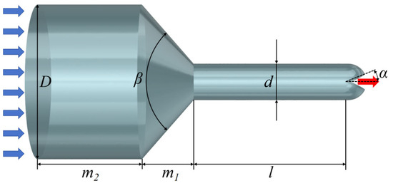
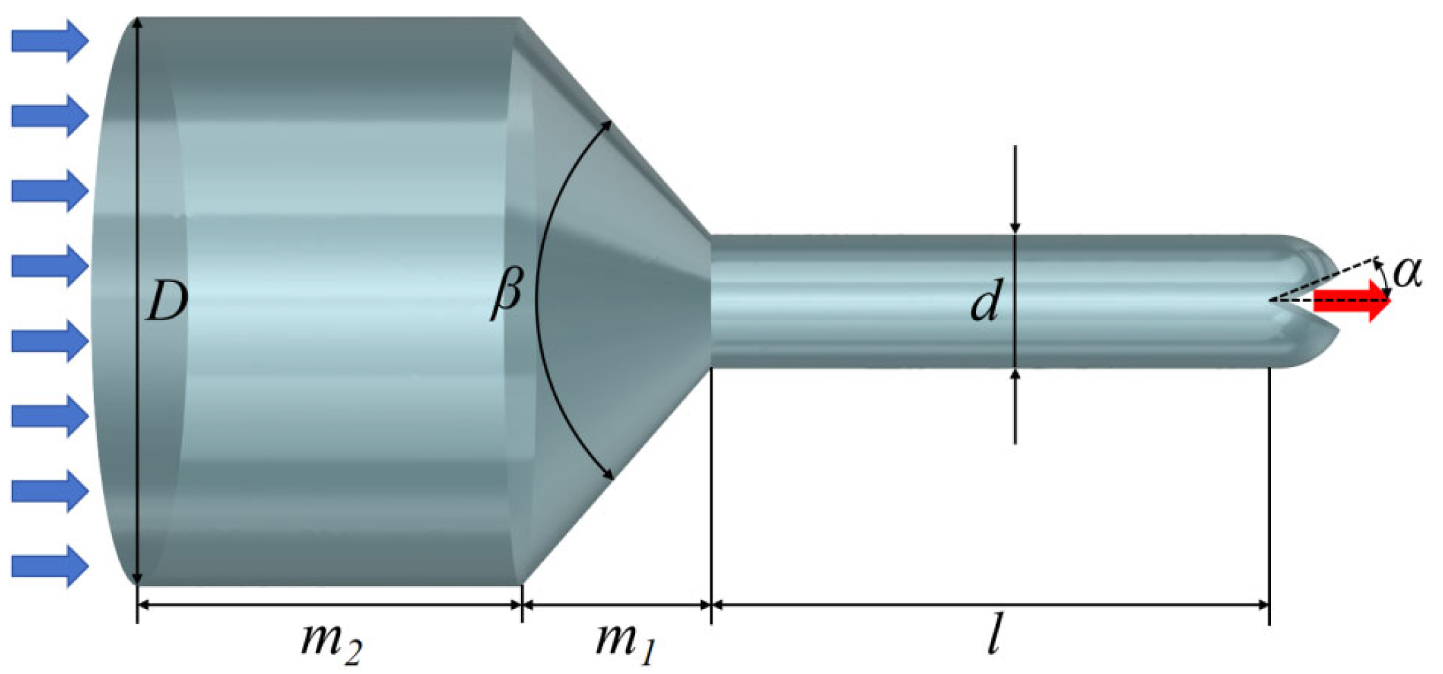
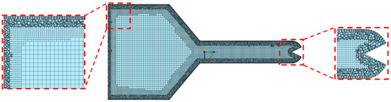
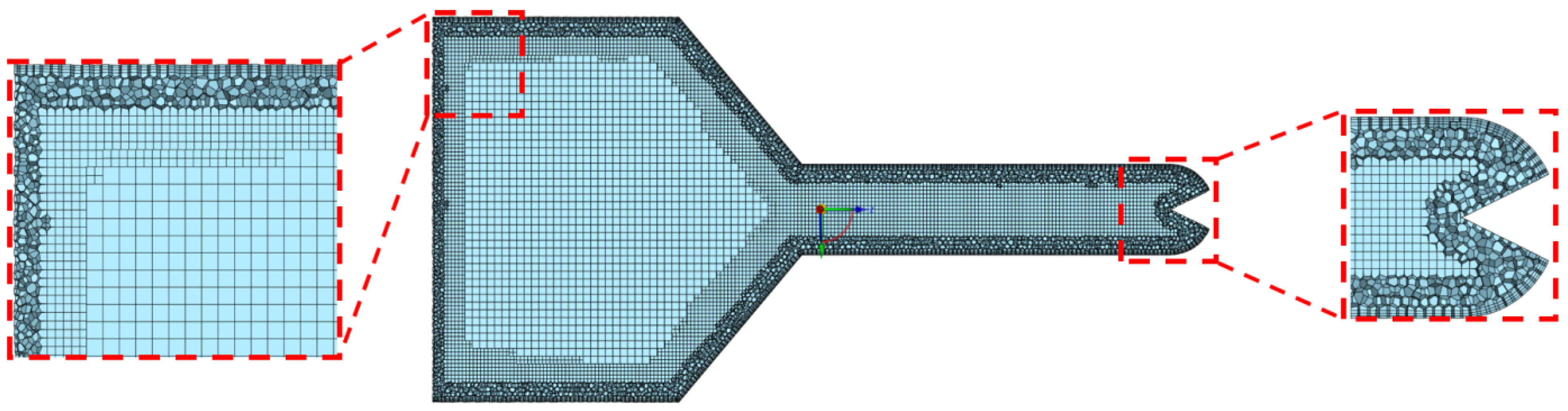
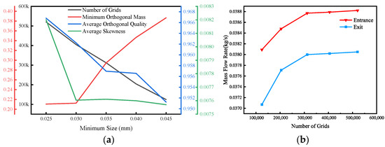
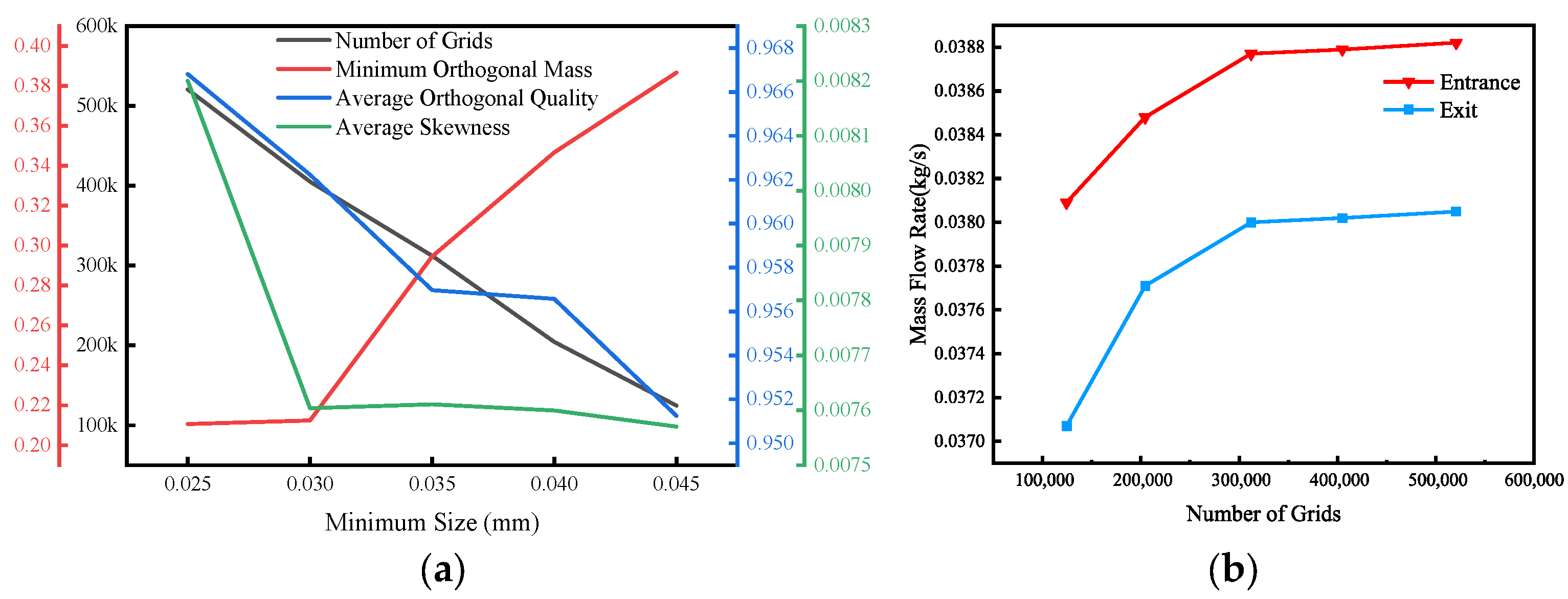
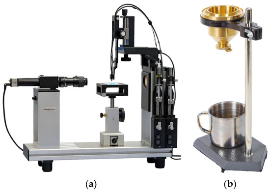
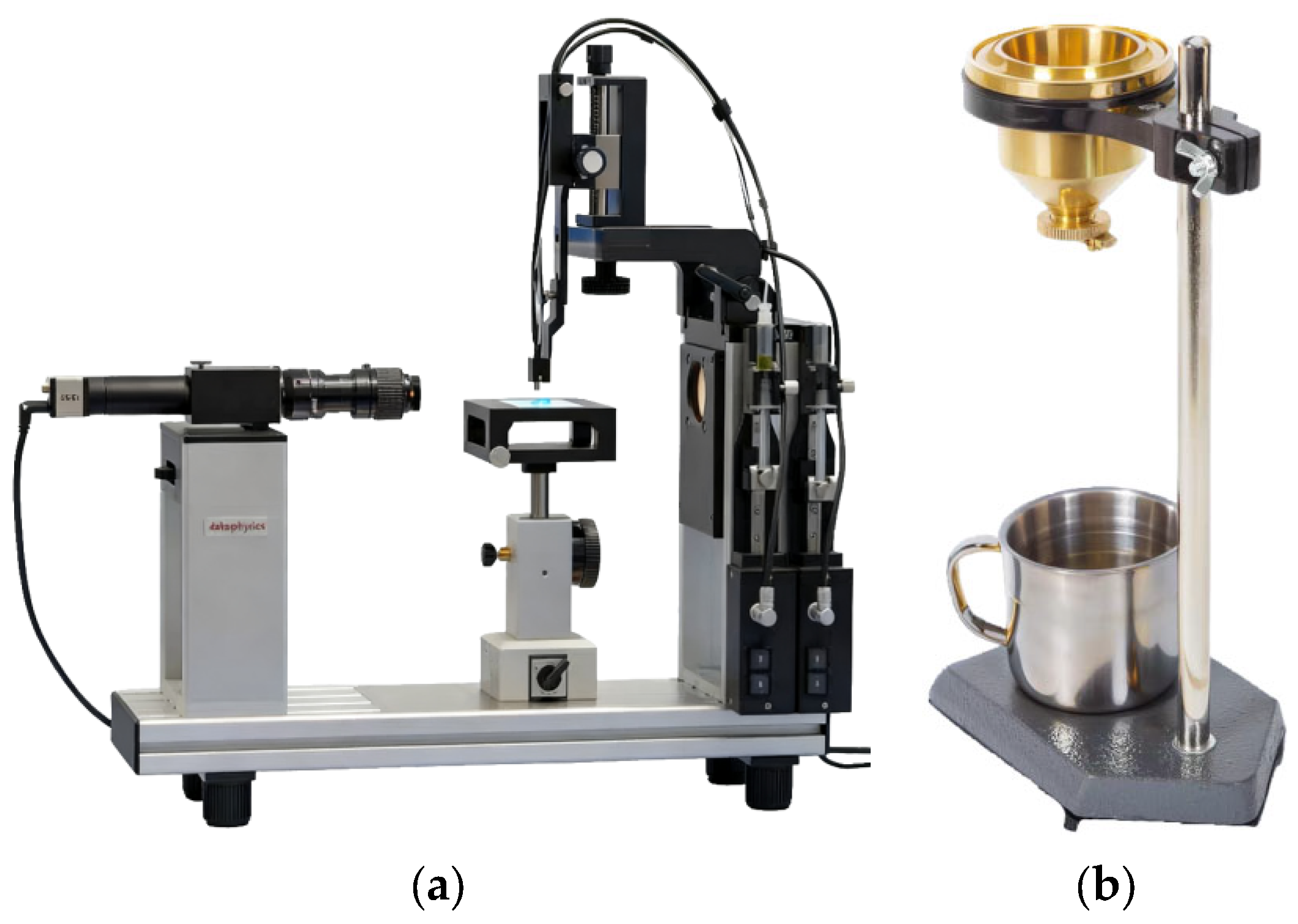
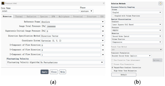
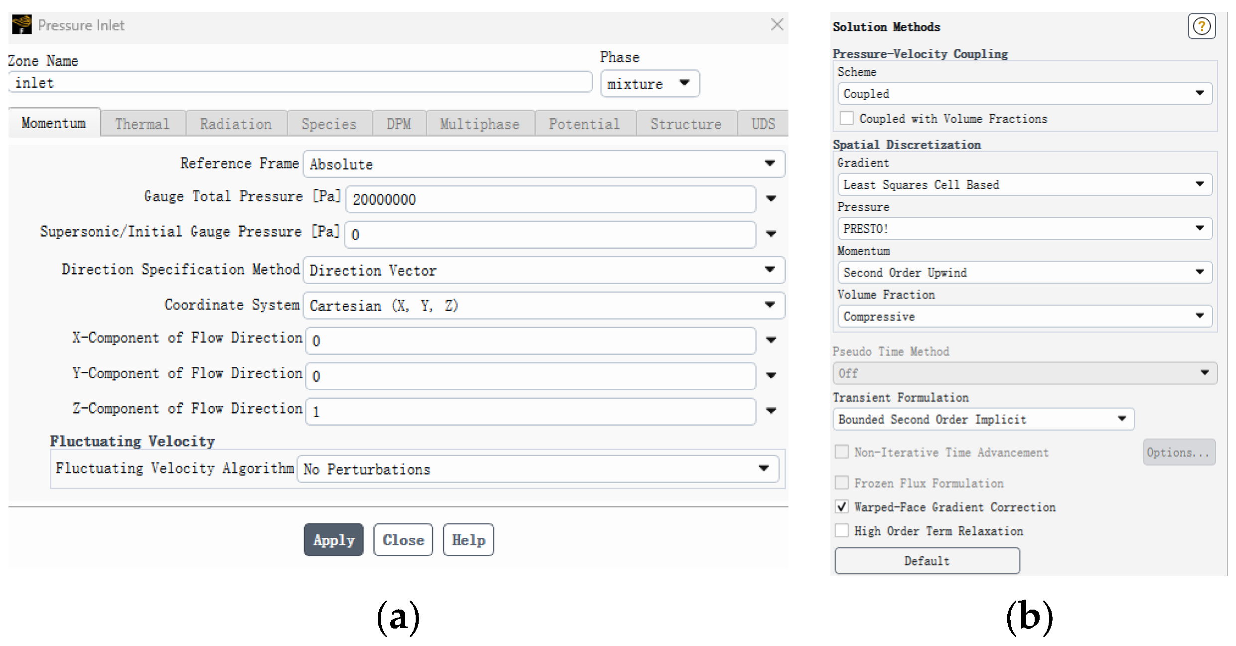
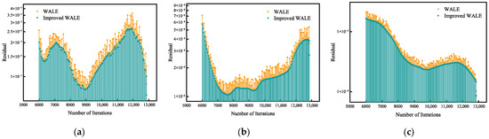
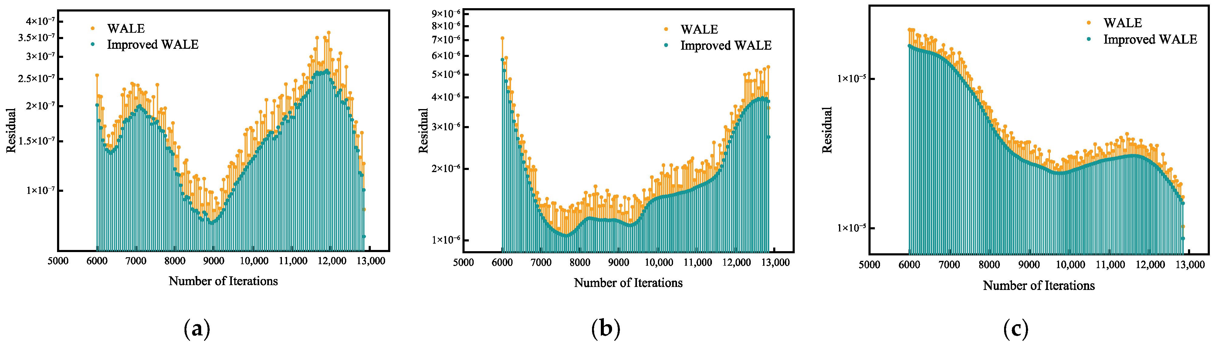
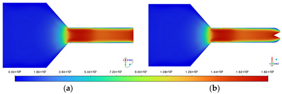
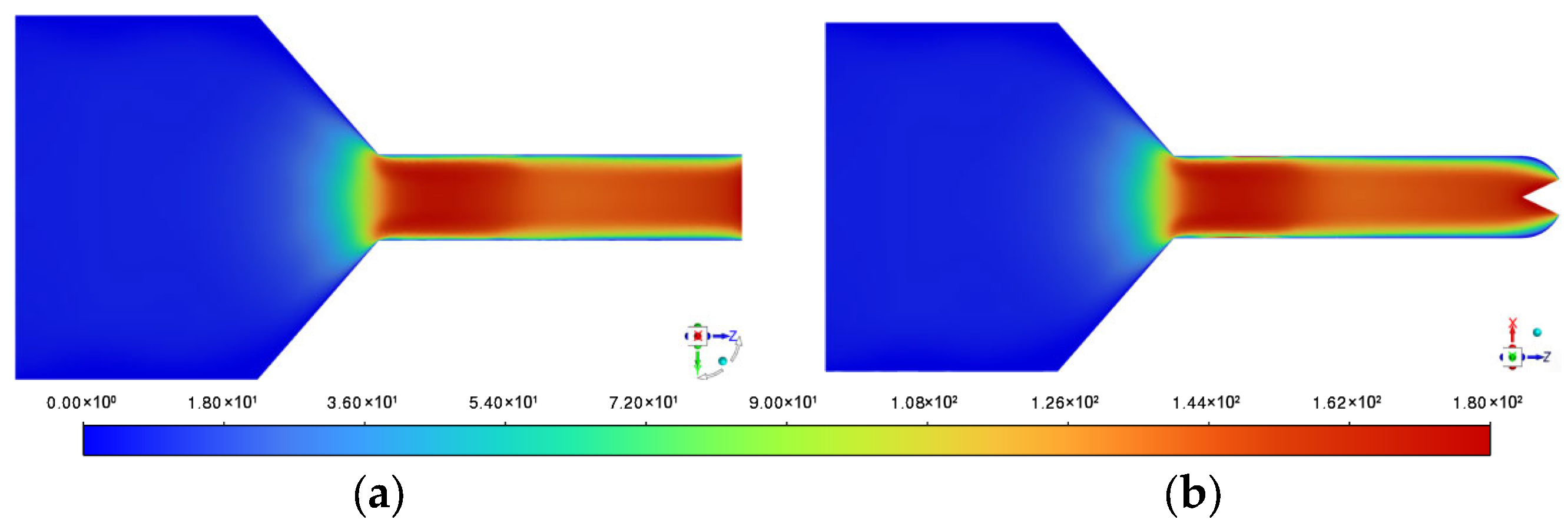
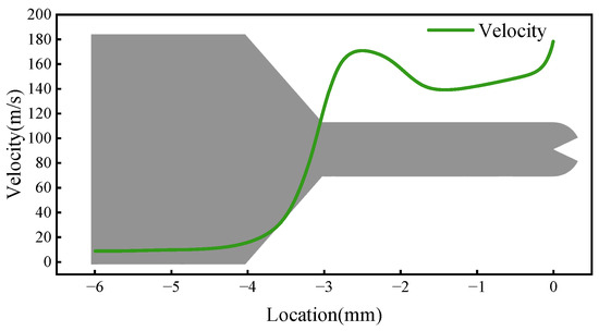
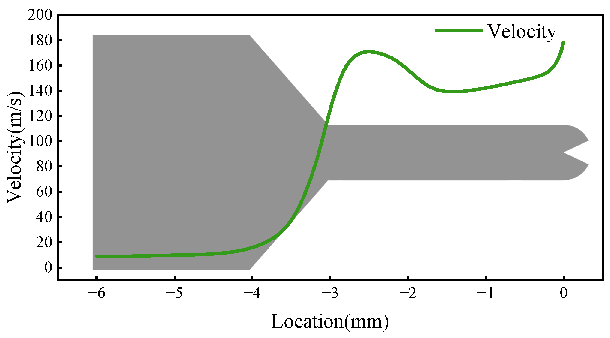
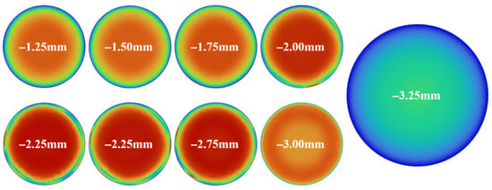
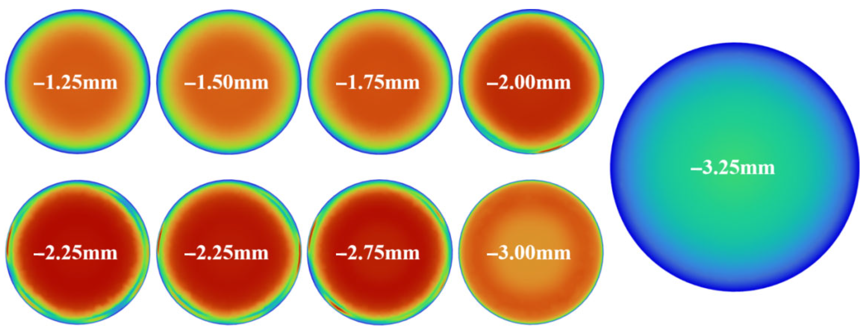
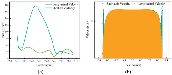
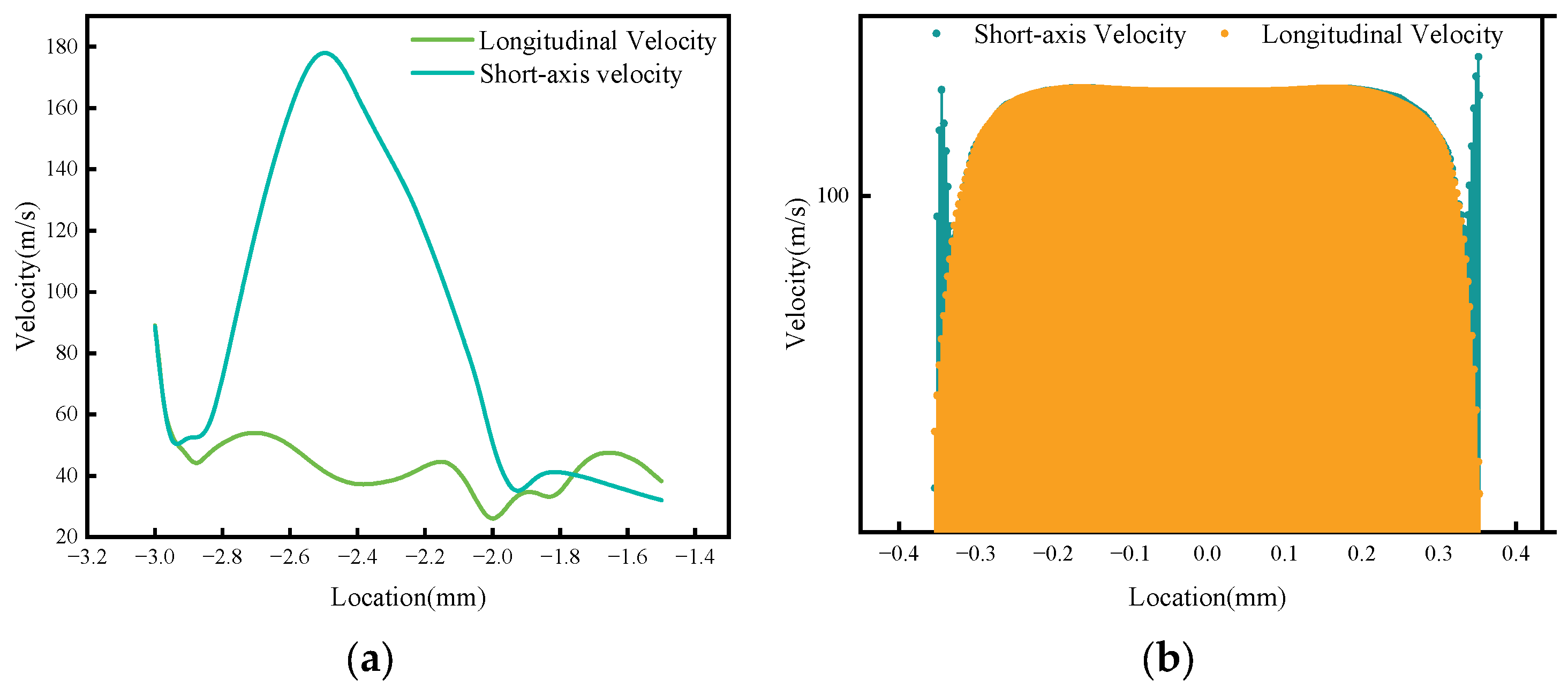
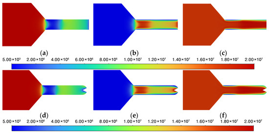
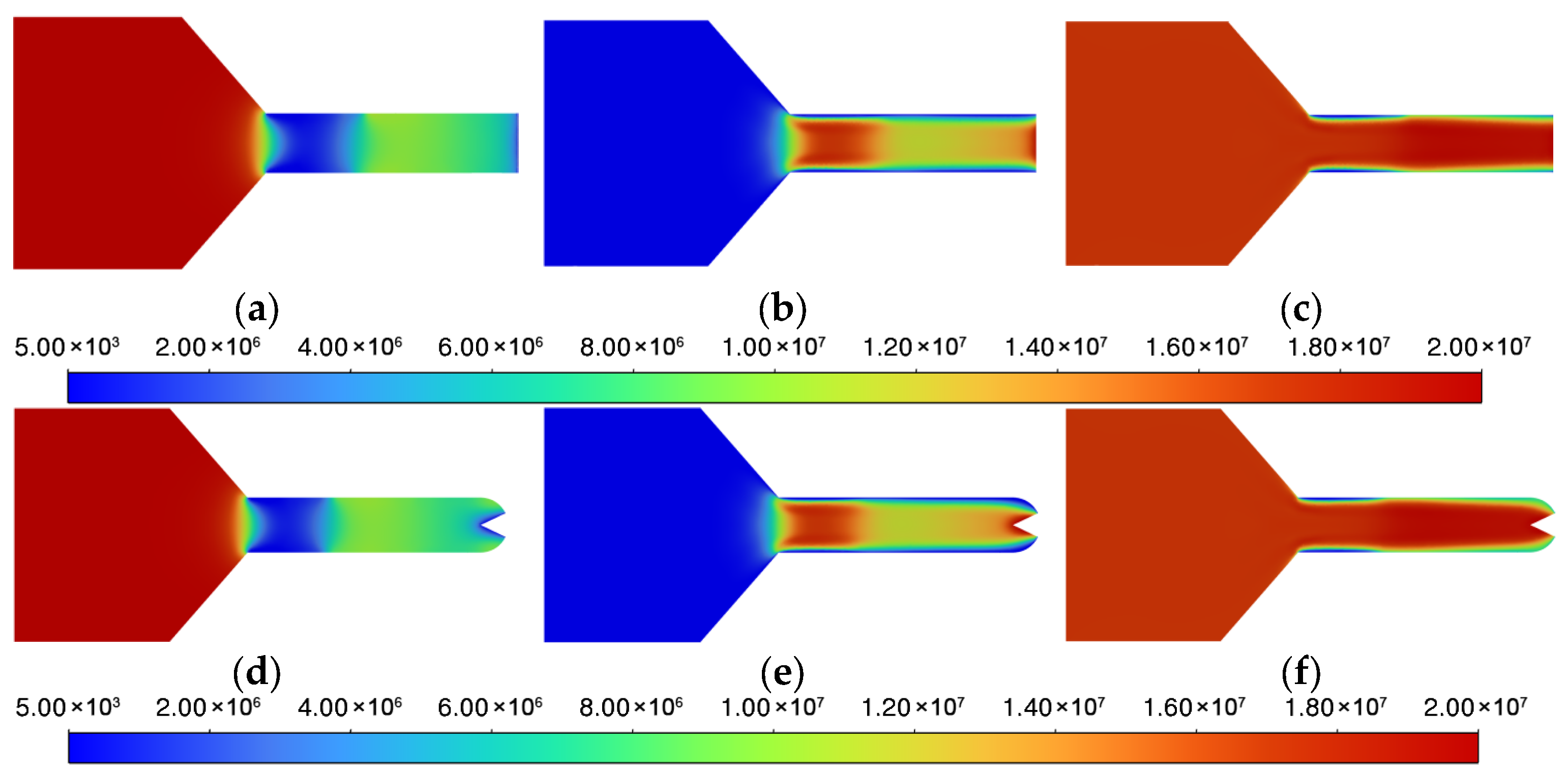
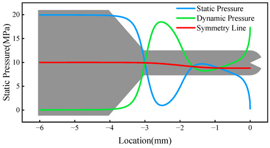
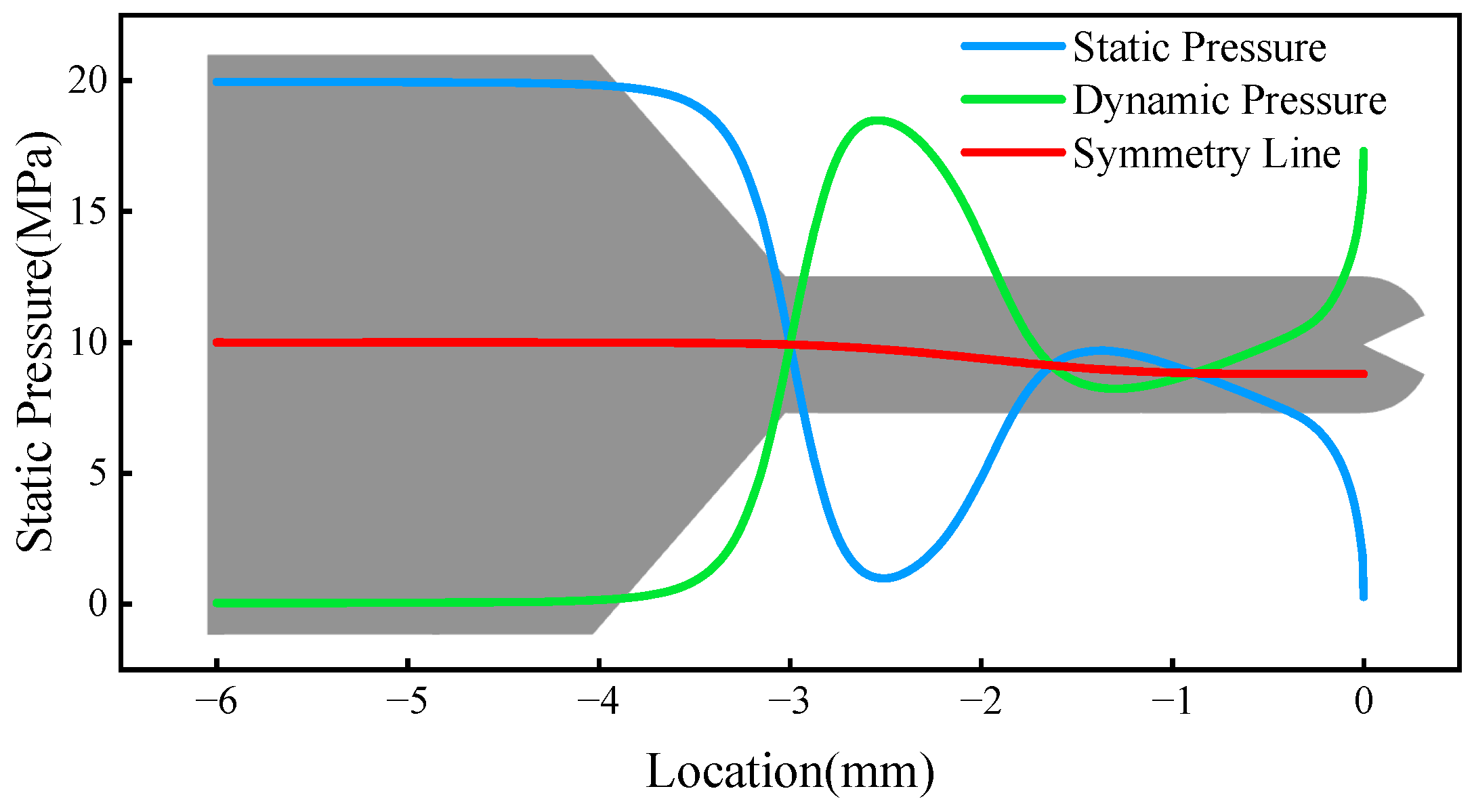
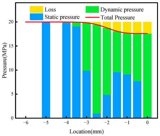
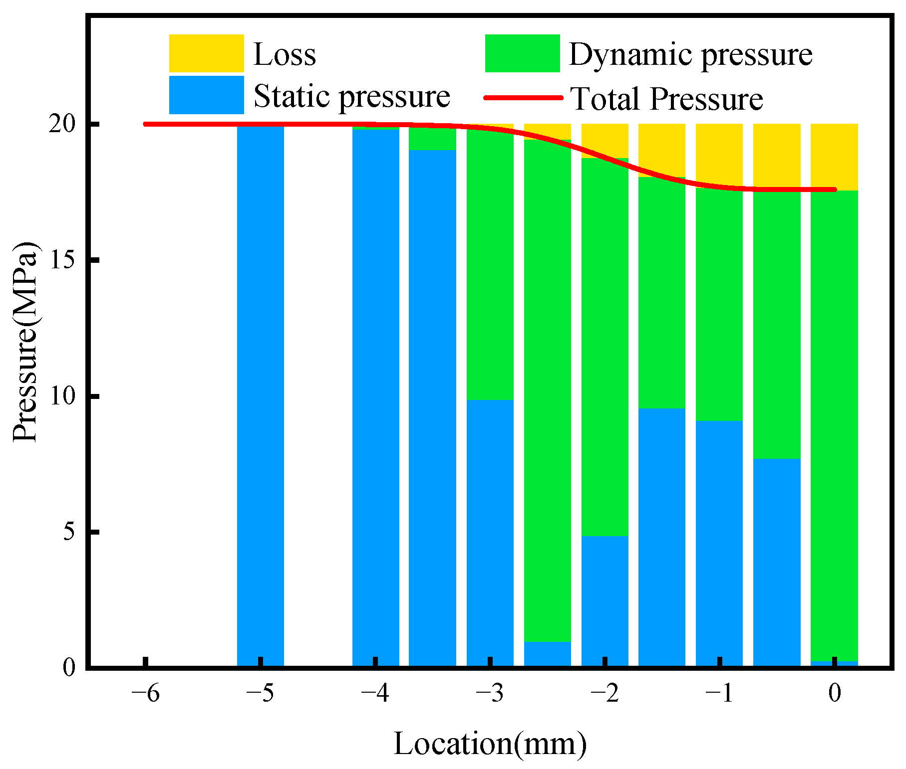
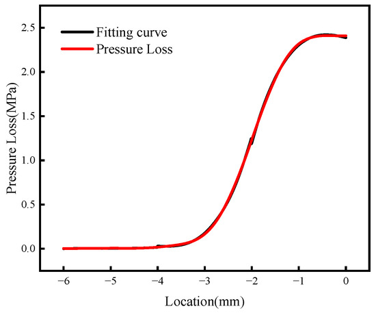
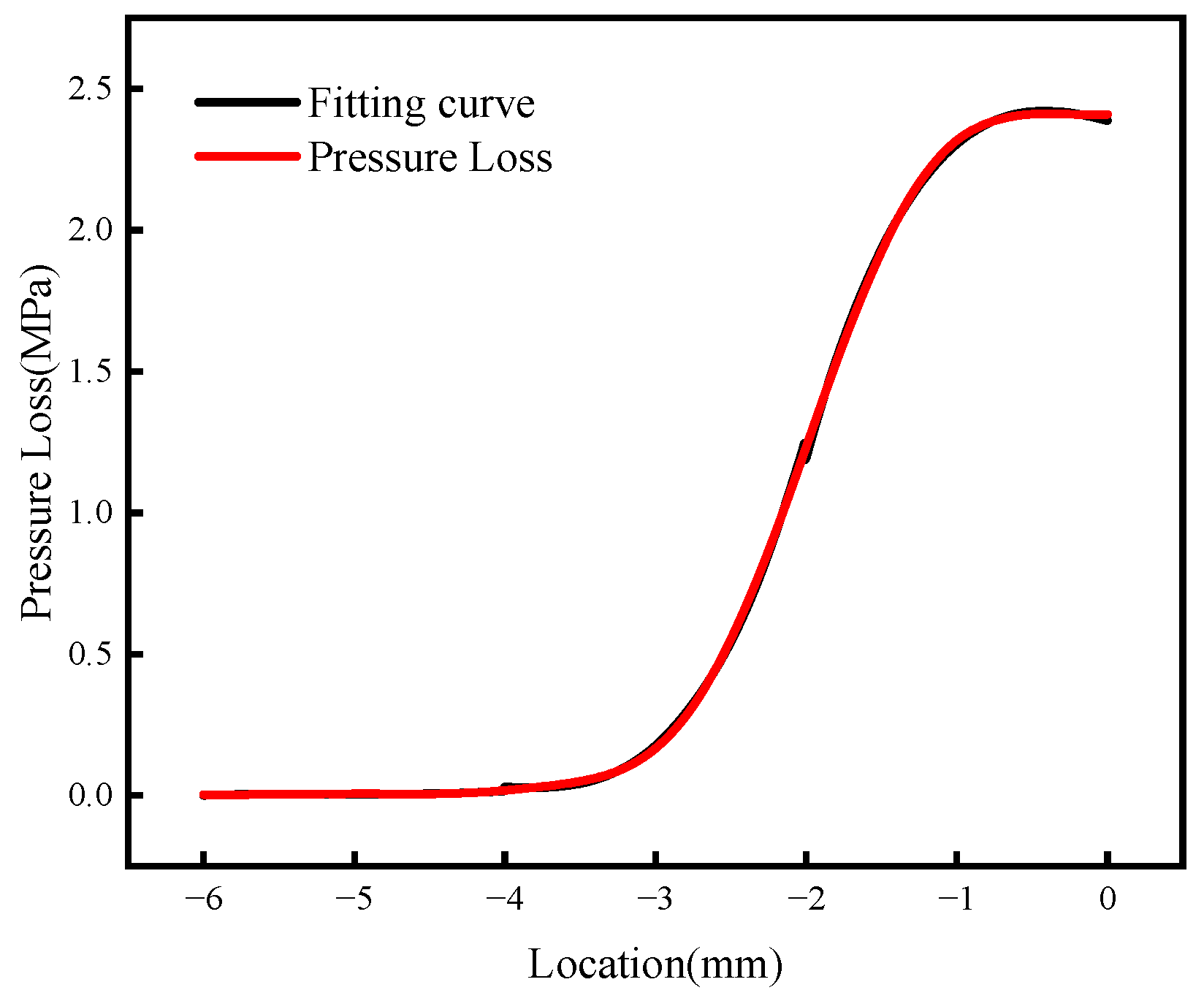
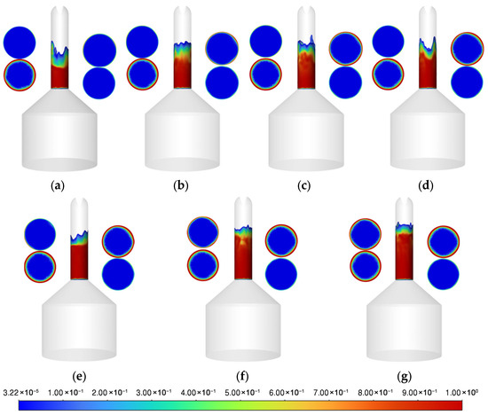
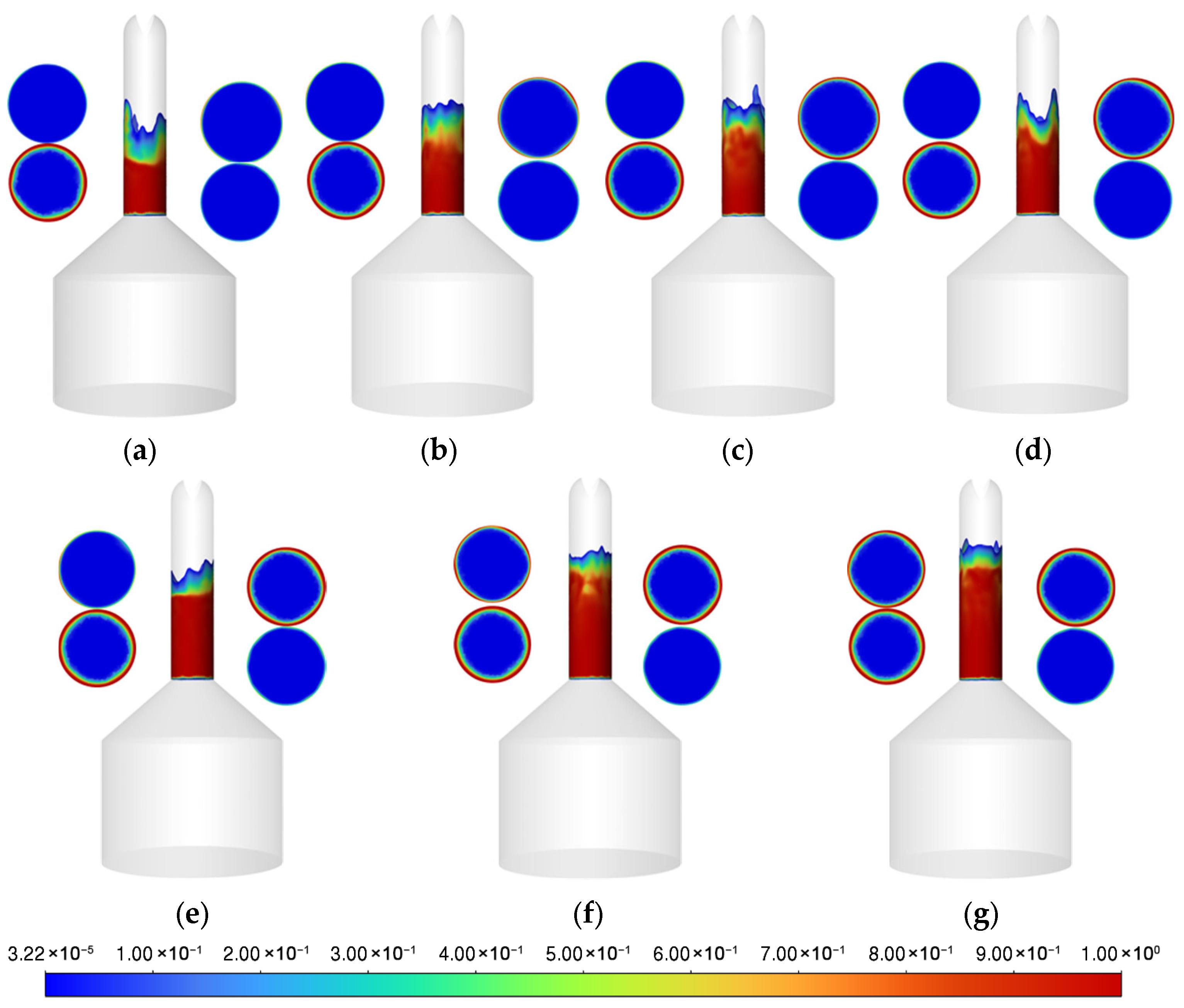
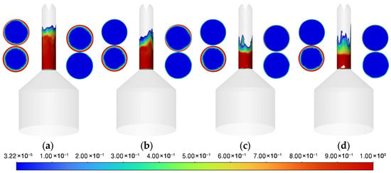
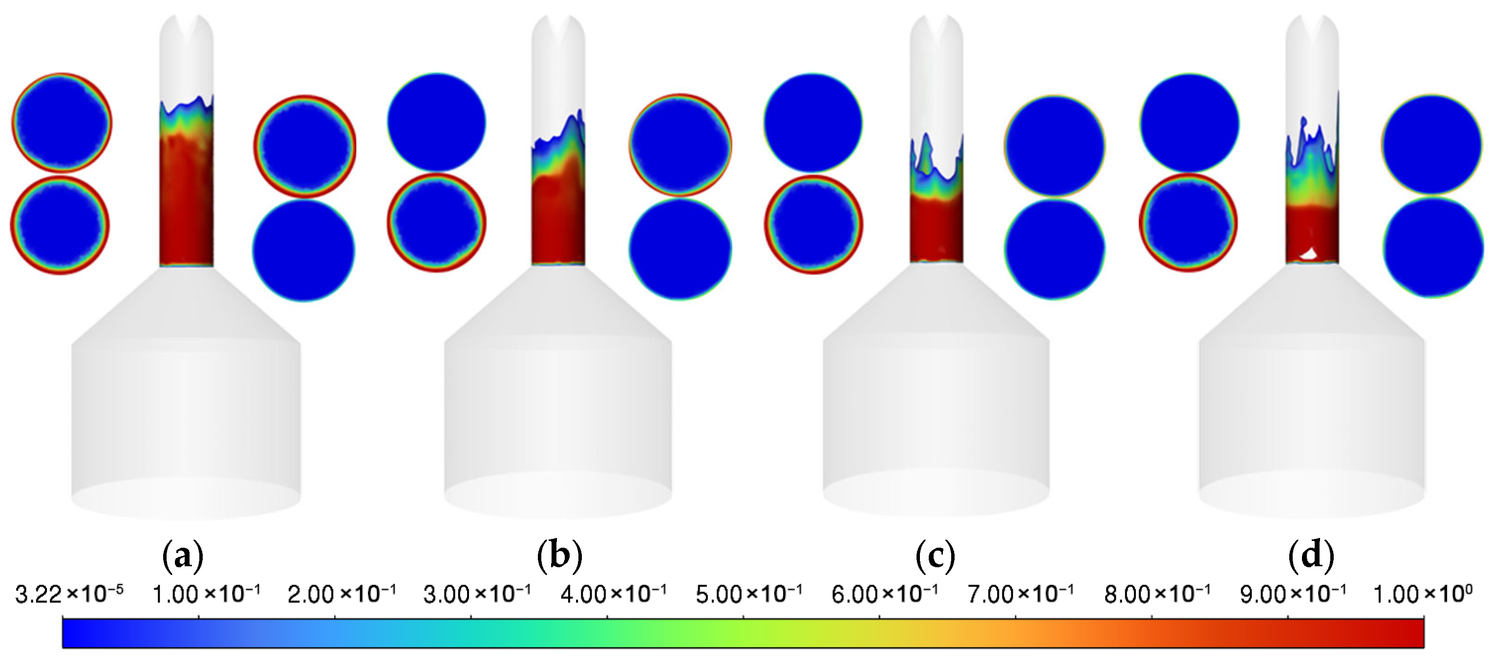
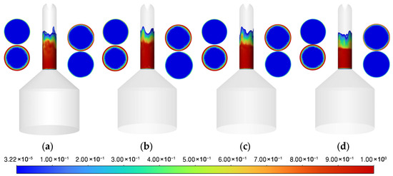
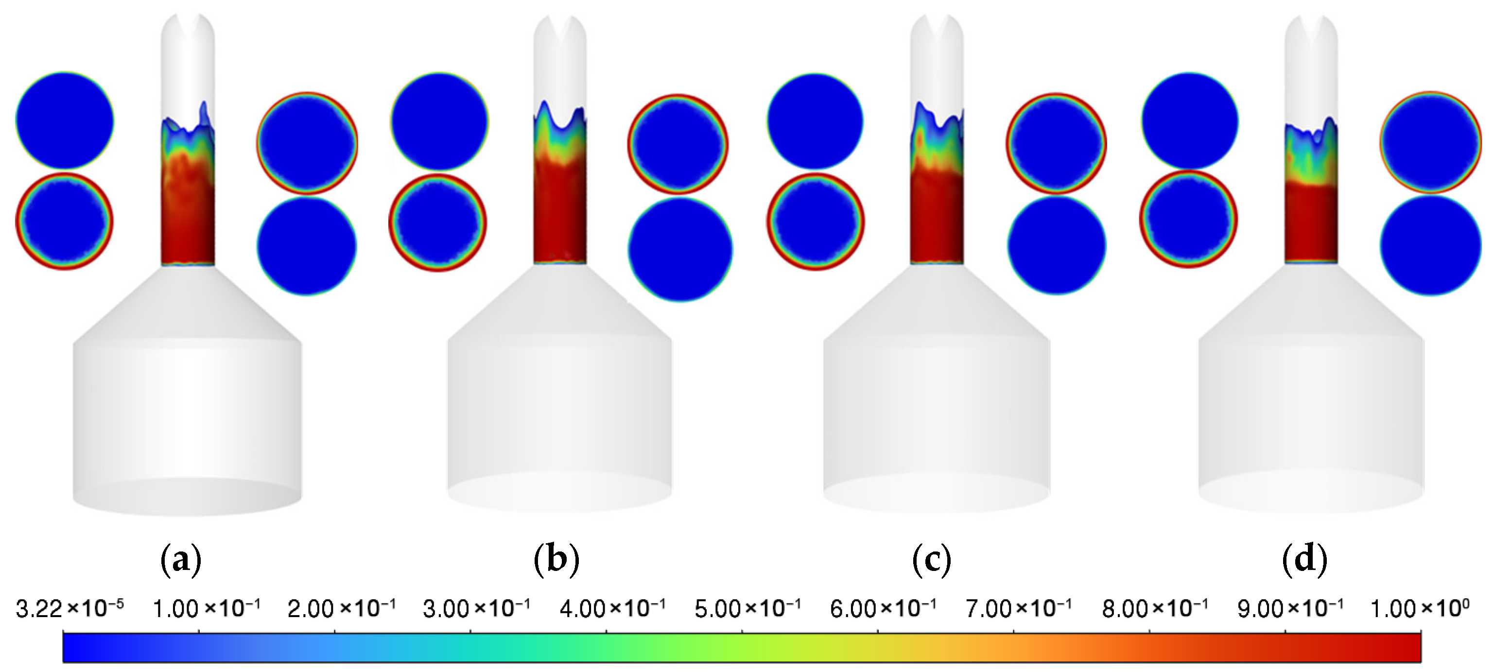
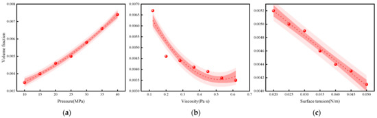
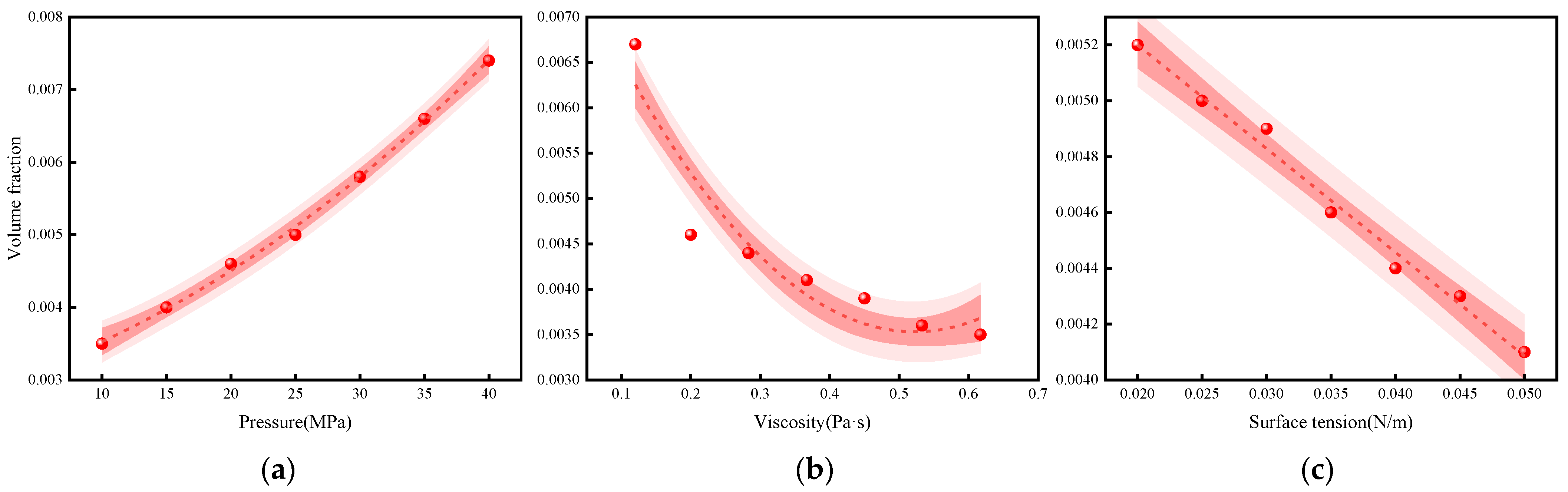
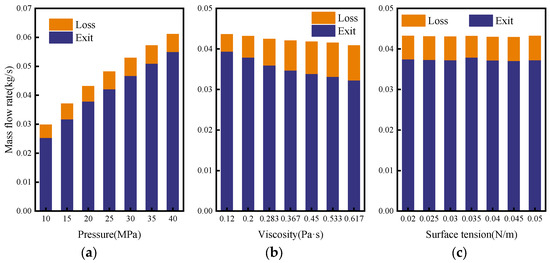
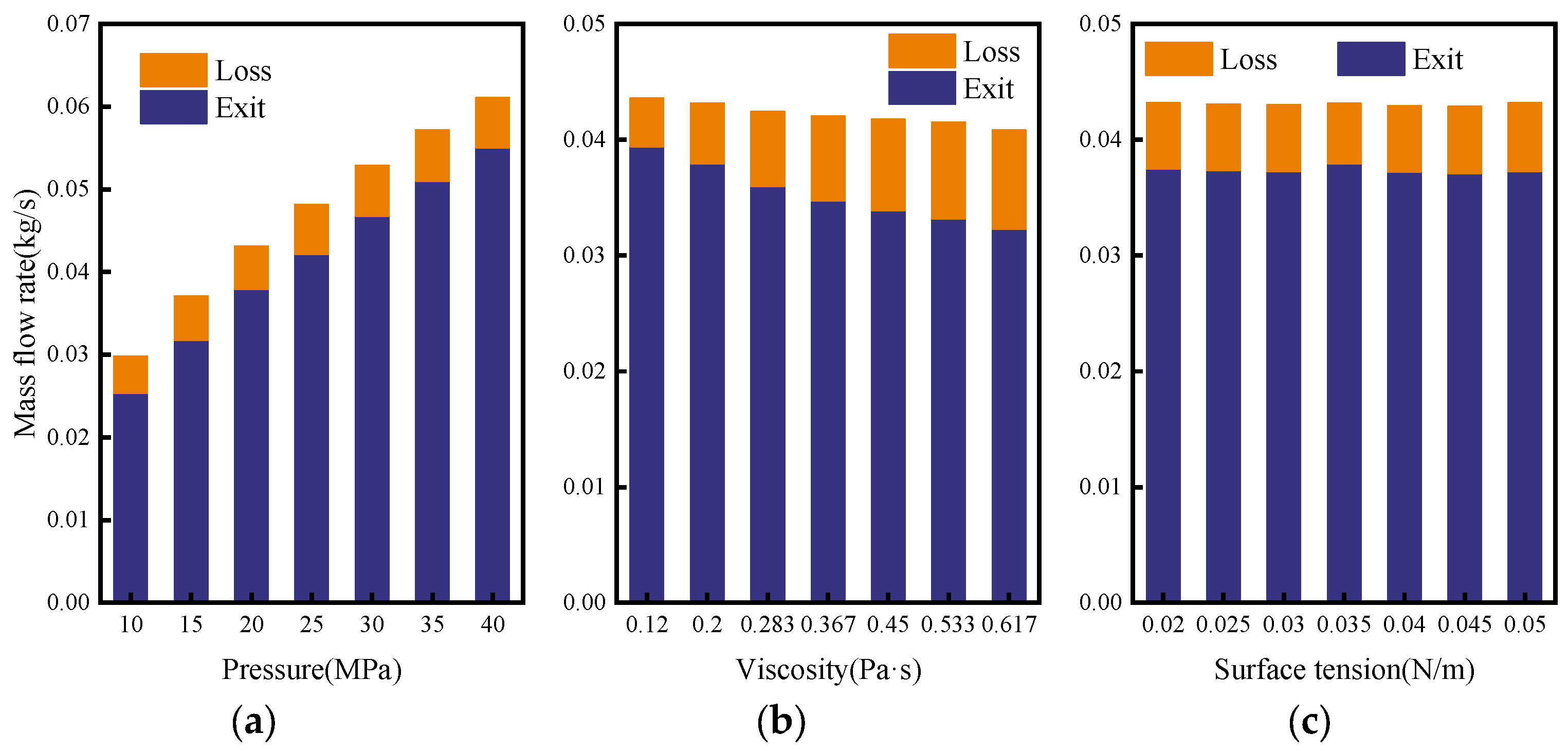
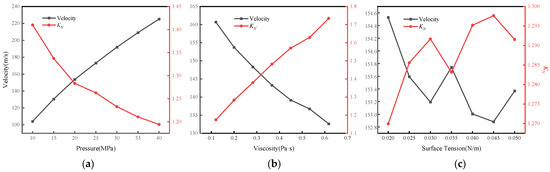
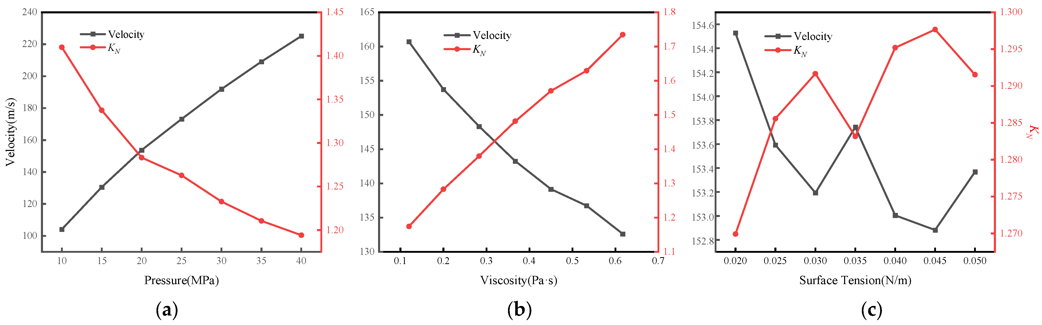
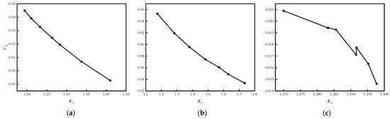
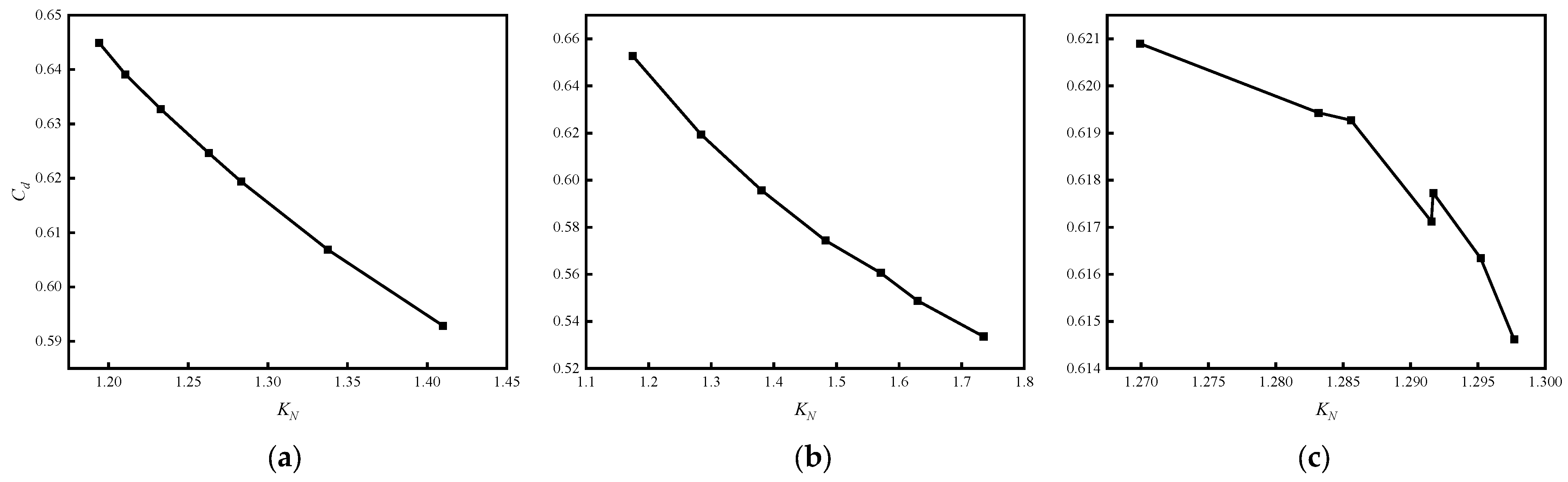
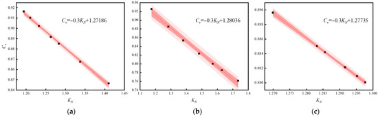
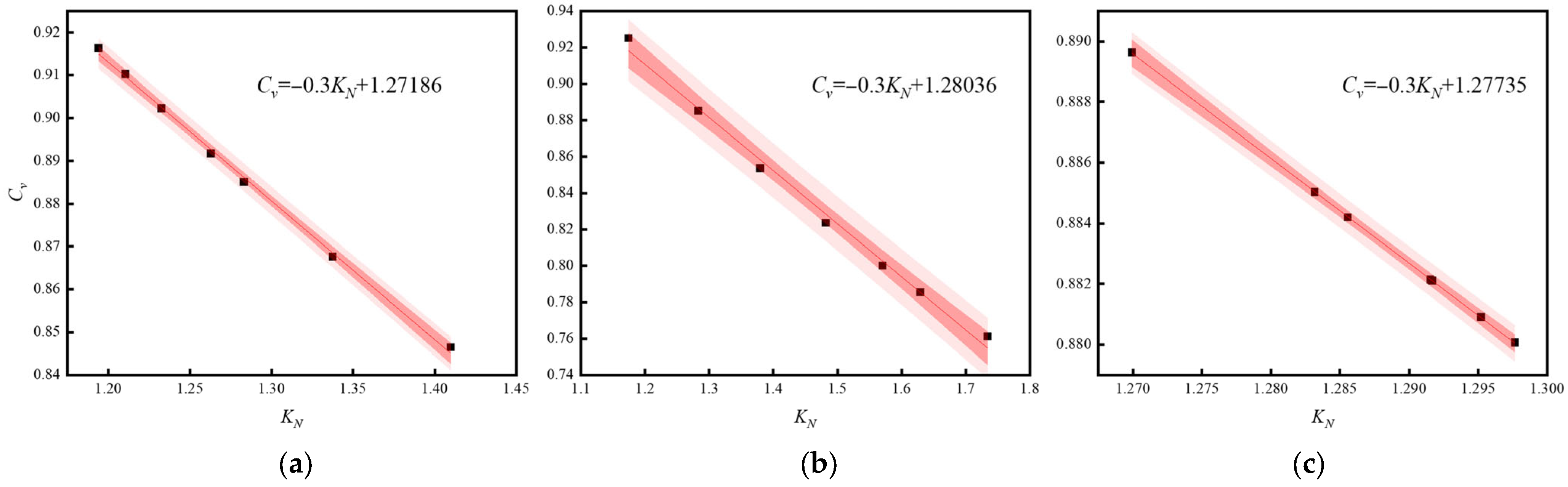
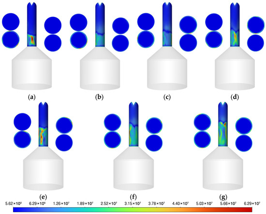
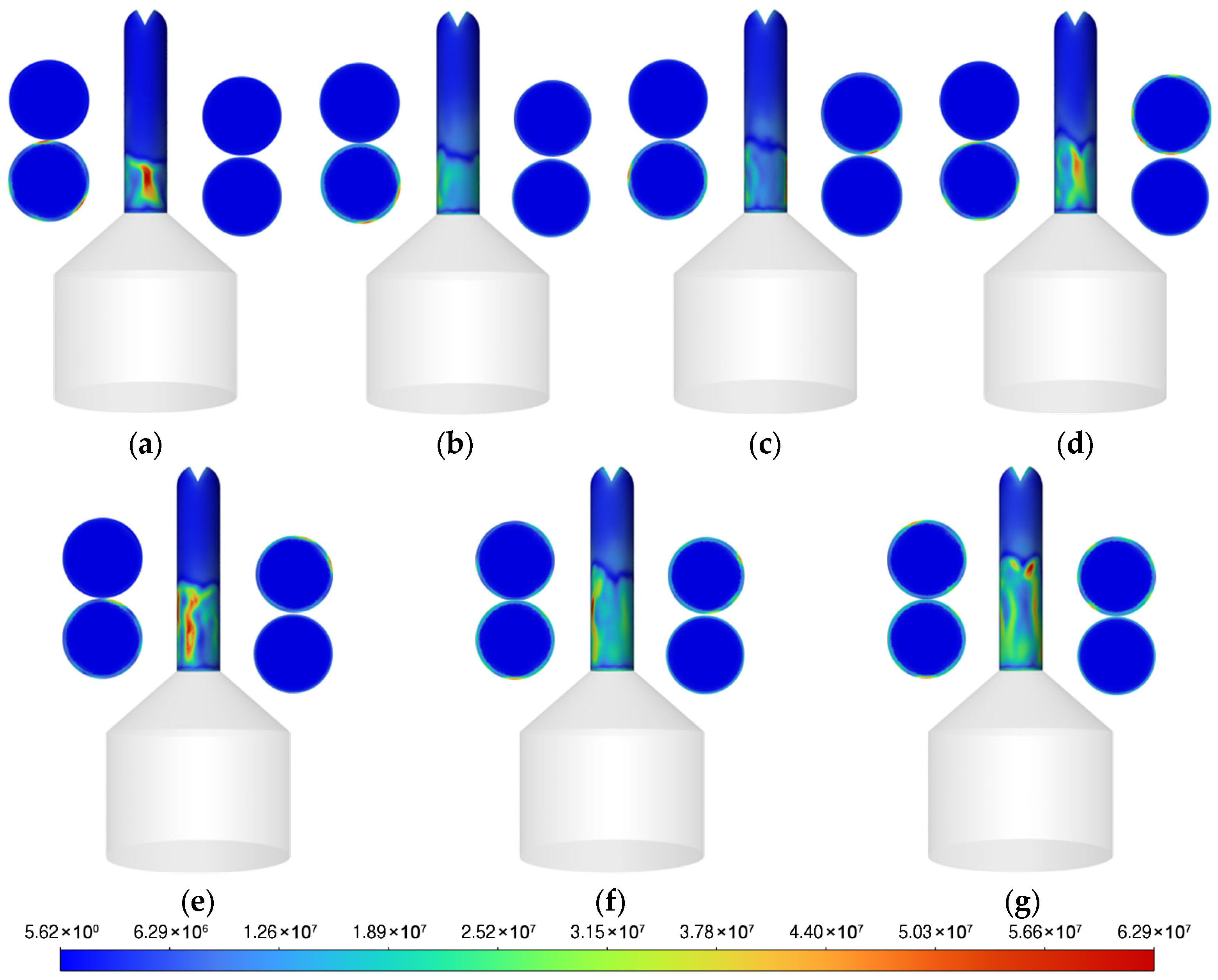
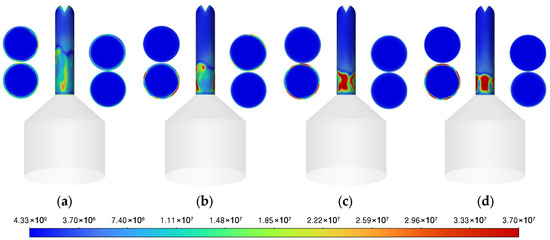
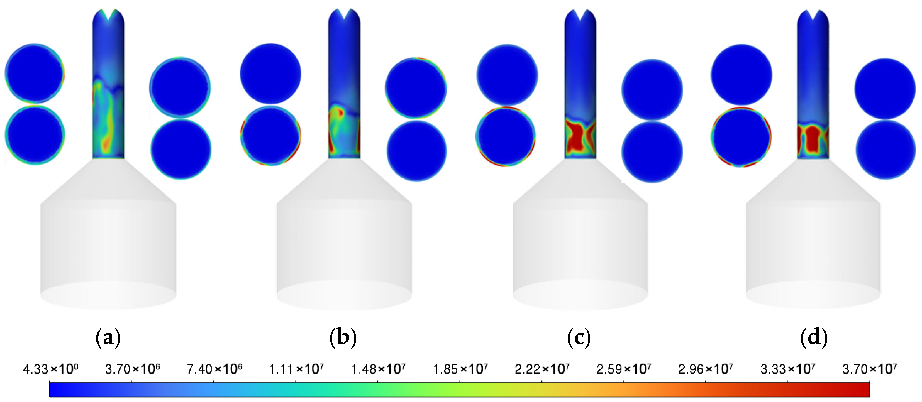
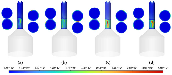
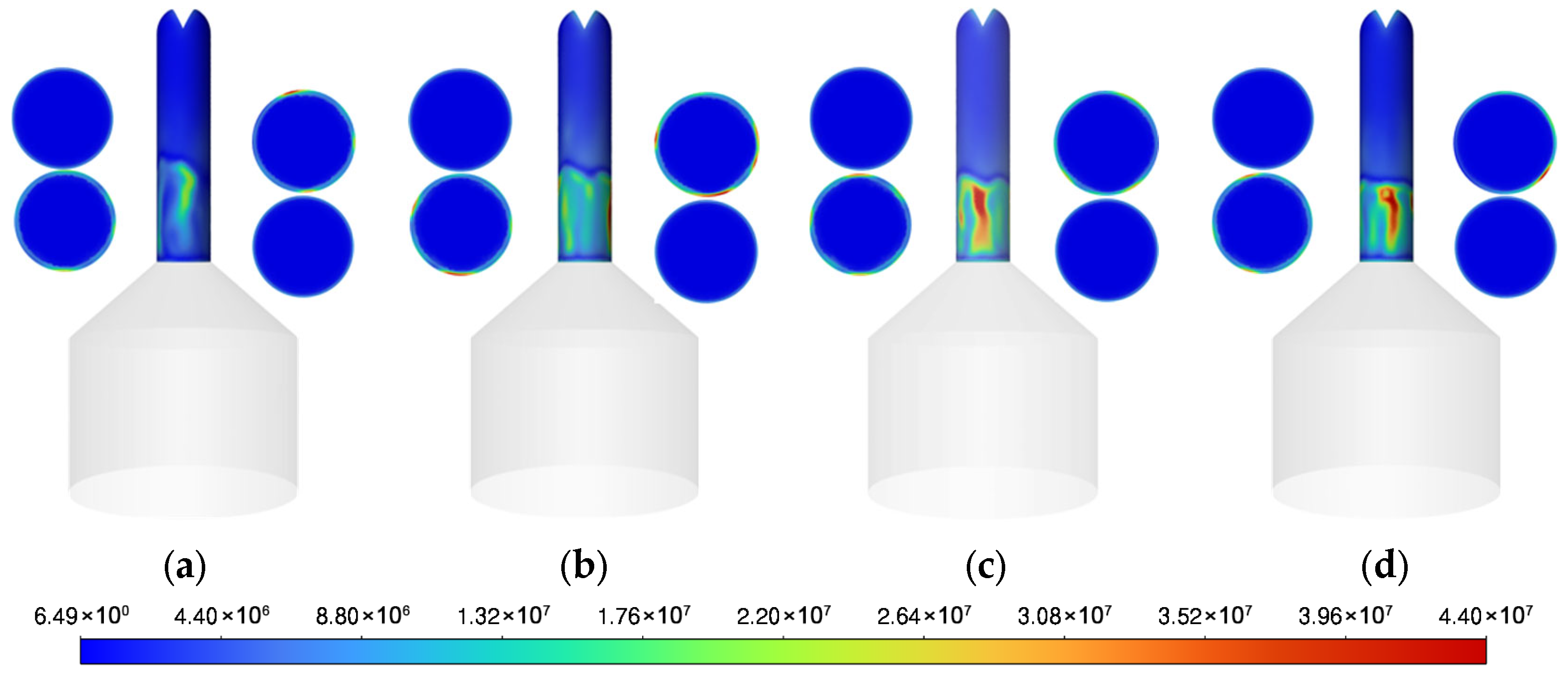
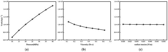
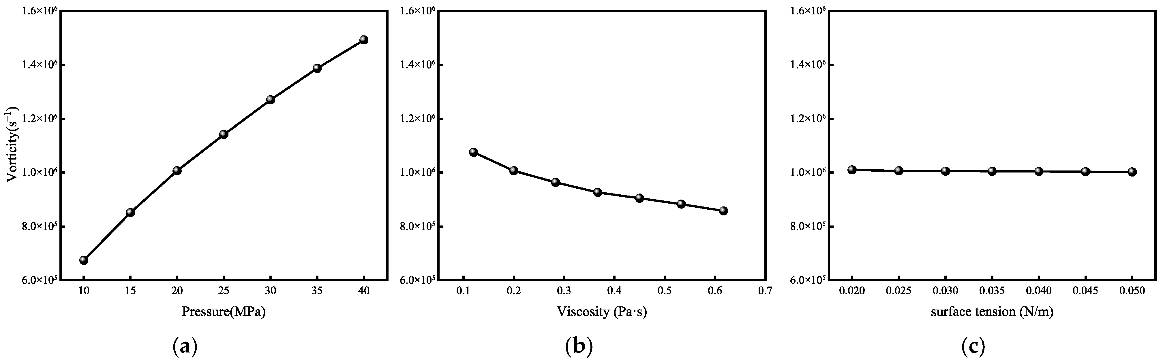
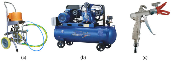
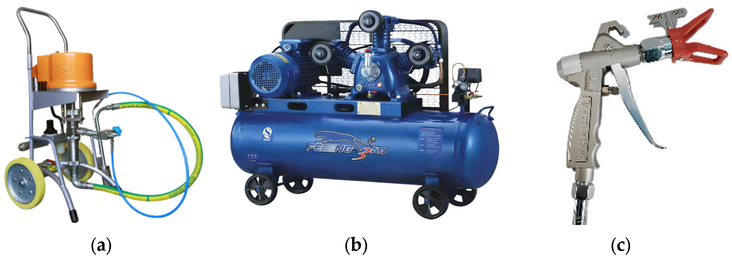
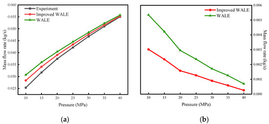
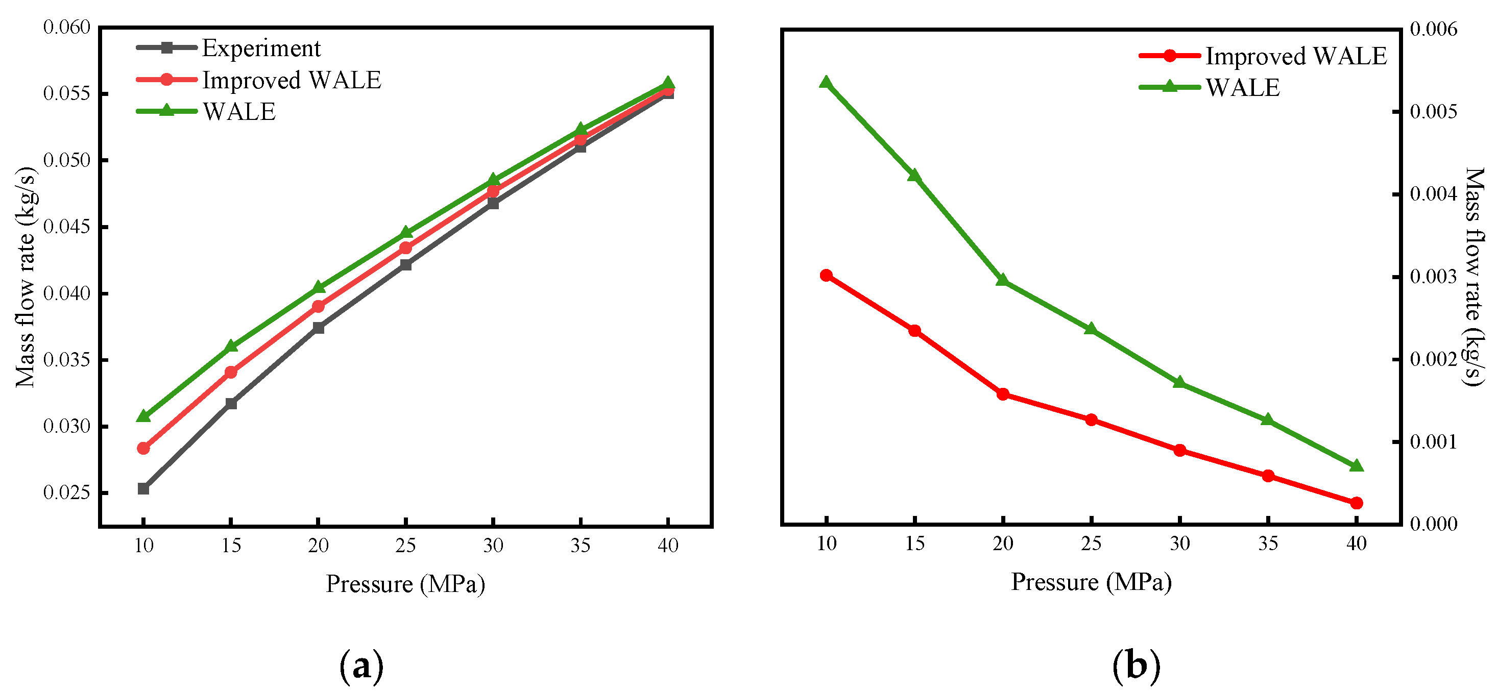

Disclaimer/Publisher’s Note: The statements, opinions and data contained in all publications are solely those of the individual author(s) and contributor(s) and not of MDPI and/or the editor(s). MDPI and/or the editor(s) disclaim responsibility for any injury to people or property resulting from any ideas, methods, instructions or products referred to in the content. |
© 2026 by the authors. Licensee MDPI, Basel, Switzerland. This article is an open access article distributed under the terms and conditions of the Creative Commons Attribution (CC BY) license.