Prediction and Interpretability Analysis of Creep in Recycled Aggregate Concrete Using Multiple Machine Learning Models

Abstract

Compared with natural aggregate concrete, the creep behavior of recycled aggregate concrete (RAC) is a key technical bottleneck restricting its engineering application. Owing to the coupled effects of multiple key factors related to recycled aggregates, RAC exhibits pronounced complexity and strong nonlinearity in its creep behavior. In this study, eight key factors were selected as input parameters, and five machine learning models were established. An online graphical user interface (GUI) prediction system based on the optimal model was developed in Python 3.9.7 using Streamlit. Furthermore, the SHapley Additive exPlanations (SHAP) method was employed to clarify the importance ranking and model-based contribution patterns of the key input factors. The results indicate that, based on four evaluation metrics, including the coefficient of determination, root mean square error, mean absolute error, and mean absolute percentage error, the back-propagation neural network (BPNN) model demonstrates superior predictive performance to the other four machine learning models across both the training and test sets, with the radial basis function neural network (RBFNN) model ranking second. The maximum coefficient of determination of the conventional RAC creep prediction models was only 0.7045, and their prediction accuracy was lower than that of all five machine learning models established in this study.

1. Introduction

With the acceleration of urbanization, the large-scale generation of waste concrete has imposed dual pressures on resources and the environment. Recycled aggregate concrete (RAC), which enables the resource utilization of waste concrete, can reduce the demand for natural aggregate exploitation and alleviate the pressure of solid waste disposal to a certain extent. Therefore, its mechanical properties, design methods, and related aspects have been widely investigated [1,2,3]. In contrast, the creep of RAC under long-term loading continuously amplifies member deformation, thereby affecting prestress loss, crack development, deflection control, and structural service safety, and is one of the key long-term properties in engineering design and durability assessment [4,5]. Considering the gradually increasing proportion of RAC in engineering applications, its creep behavior and predictability should be incorporated into the framework of long-term performance control to support safe and reliable design.

Existing studies have generally demonstrated that, under similar strength grades, loading conditions, and environmental conditions, the creep development of RAC is broadly similar to that of natural aggregate concrete (NAC). Both materials exhibit rapid creep growth at the early stage, followed by a gradual deceleration and eventual stabilization of creep deformation [6,7]. Meanwhile, due to the unique multiphase characteristics of recycled aggregates, the residual old mortar attached to aggregate surfaces generally features a low elastic modulus, high porosity and abundant initial defects. These inherent defects reduce the overall elastic modulus of RAC and increase its susceptibility to long-term deformation [8,9]. Therefore, under the same loading and environmental conditions, the creep deformation of RAC is generally higher than that of ordinary concrete [10,11,12]. Furthermore, for specimens with identical mix proportions and loading conditions, this incremental creep trend becomes more prominent with the rise in recycled aggregate replacement ratio [13,14,15]. Specifically, the creep deformation of RAC can increase by approximately 50% when natural aggregates are fully replaced by recycled aggregates [16]. Therefore, it is particularly necessary to systematically research the creep evolution law and influencing mechanisms of RAC.

Regarding the influencing factors of RAC creep behavior, Liu et al. demonstrated that creep behavior is strongly influenced by factors such as the stress-to-strength ratio, cement content, and mineral admixture content, and that it exhibits significant nonlinear characteristics [17]. In addition, the water-to-cement ratio, aggregate properties, age, humidity, temperature, and other factors also have certain effects on creep [18,19,20]. At present, the commonly used method for determining concrete creep is experimental testing. However, such tests require a long duration and considerable investments of manpower and material resources. If reliable and effective concrete creep prediction models can be established, experimental testing can be avoided and work efficiency can be improved [21,22,23]. In recent years, machine learning techniques have demonstrated excellent capability in predicting the mechanical properties of concrete materials, and have been widely adopted for the modeling of concrete mechanical performance [24,25,26], durability [27,28,29], and other indicators. Existing studies have verified that machine learning-based models possess prominent advantages in handling multivariate and nonlinear relationships, and generally provide more accurate predictions than conventional empirical formulas and regression models [30,31]. In addition, machine learning methods exhibit high adaptability in characterizing the complex multi-factor coupling behavior of concrete, which provides a solid theoretical and technical foundation for predicting time-dependent long-term material properties.

Creep is a typical long-term mechanical property of both NAC and RAC, and numerous machine learning models have been increasingly adopted to predict creep. Liang et al. investigated concrete creep based on ensemble learning models, including random forest and gradient boosting. The results demonstrated that machine learning models exhibit substantially higher creep prediction accuracy than conventional empirical models. They also identified loading time, compressive strength, loading age, relative humidity, and temperature as the main influencing factors [32]. Other comparative studies on artificial neural networks and support vector regression based on diverse databases revealed that support vector regression can achieve superior prediction accuracy under specific data scenarios [33]. For complex service environments such as elevated temperatures, machine learning algorithms including artificial neural networks, random forest, linear regression and Gaussian process regression can effectively characterize concrete creep behavior. In particular, linear regression and Gaussian process regression outperform conventional empirical equations under certain conditions [34]. For RAC creep prediction, Gao et al. established data-driven models based on back-propagation neural network, whale optimization algorithm, and extreme gradient boosting. Using a comprehensive database of 291 sets of RAC creep test data, they verified the reliability of the optimized learning algorithms and parameter importance analysis [35]. Feng et al. systematically compared five classic machine learning algorithms via the RAC_Creep_v1 database, and concluded that extreme gradient boosting serves as a high-accuracy and high-efficiency model for RAC creep prediction [36]. Rong et al. established RAC creep prediction models using back-propagation neural network and support vector machine based on a database containing 15 parameters and 1309 data points, which exhibited superior prediction performance to conventional RAC creep models [37]. Although existing studies have validated the promising applicability of machine learning methods in predicting the creep behavior of NAC and RAC, the optimal performance of different models remains inconclusive. Such discrepancies mainly stem from inconsistent data sources, variable input parameter selection and diverse evaluation metrics adopted in existing research.

Accordingly, this study focuses on the creep behavior of RAC. Eight key influencing parameters are selected as input parameters to establish five machine learning models, including back-propagation neural network (BPNN), radial basis function neural network (RBFNN), support vector regression (SVR), random forest (RF), and gene expression programming (GEP). The prediction performance of the five models is systematically compared based on a unified database and evaluation metric system. To satisfy the prediction demands of practical engineering, a web-based graphical user interface (GUI) prediction system is developed using Python 3.9.7 and the Streamlit framework based on the optimal machine learning model. In addition, SHapley Additive exPlanations (SHAP)-based interpretability analysis is performed on the optimal model to evaluate the contribution of each input parameter and elucidate the corresponding working mechanisms. Finally, the established machine learning models are compared with three conventional RAC creep models to verify their superior prediction performance. The proposed prediction framework can provide a reliable reference for the long-term performance assessment and engineering application of RAC structures.

2. Database Analysis and Evaluation Metrics

2.1. Selection of Input Parameters

To achieve accurate machine-learning-based prediction and analysis of RAC creep behavior, eight key influencing parameters were statistically screened as model parameters, including ordinary Portland cement content (Y₁), sand ratio of RAC (Y₂), water-to-binder ratio of RAC (Y₃), water absorption of mixed coarse aggregates (Y₄), humidity of the creep test (Y₅), compressive strength (Y₆), stress ratio (Y₇), and creep test time (Y₈). These parameters were used to establish five machine learning models, with the specific creep of RAC defined as the corresponding output parameter (Z). The specific creep was calculated as the ratio of creep strain to the applied stress.

2.2. Database Establishment and Division

This study established a database consisting of 349 groups of RAC specific creep test data [38,39,40,41,42,43]. All data were obtained from creep tests conducted on specimens after 28 days of curing, with uniform specimen dimensions of 100 mm × 100 mm × 400 mm. The statistical characteristics of the database are summarized in Table 1. As shown by the data distribution ranges in Table 1. The selected parameters cover relatively broad variation ranges within the collected RAC creep database, which provides a reasonable basis for establishing the prediction models.

Table 1. Statistical characteristics of the input and output parameters in the RAC creep database.

Parameter	Maximum	Minimum	Mean	Median	Standard Deviation
Y1/(kg/m3)	467.4	180	350.53	315	92.56
Y2	0.43	0.35	0.38	0.38	0.018
Y3	0.53	0.38	0.43	0.40	0.043
Y4/(%)	6.1	0.3	3.21	3.33	1.87
Y5/(%)	65	60	60.82	60	1.85
Y6/(MPa)	44.3	24.3	33.90	33.8	5.52
Y7	0.6	0.3	0.37	0.4	0.057
Y8/(d)	360	1	96.29	62	90.77
Z(10−6 MPa−1)	87.71	1.14	34.19	31.4	15.64

The database was randomly split into training and test sets at a ratio of 4:1, corresponding to 280 and 69 data groups, respectively. Considering the limited availability of RAC creep experimental data, random splitting was adopted to maximize the utilization of available samples. Before model training, duplicate records were carefully checked and removed to avoid direct repetition of identical samples between the training and test sets. In MATLAB R2022b, the randperm function was utilized to generate a randomized integer sequence ranging from 1 to 349. The first 280 samples were designated as the training set, and the remaining 69 samples were used as the test set. It should be noted that samples derived from the same experimental source may still exhibit certain correlations, which represents a potential limitation of the current data splitting strategy.

During the model development process, hyperparameter optimization was conducted using only the training set, and the test set was not involved in model tuning but was exclusively used for the final evaluation of model performance.

In machine learning modeling, input and output parameters need to possess adequate sample size and reliable data quality. Meanwhile, it is necessary to analyze the linear correlations among various indicators [44]. Strong linear correlations between parameters will degrade the prediction accuracy of machine learning models. The Pearson correlation coefficient is widely adopted to quantify the correlations between parameters, and its calculation formula is presented in Equation (1) [17]. The value of the Pearson correlation coefficient between any two parameters ranges from −1 to 1. A value closer to 0 indicates a weaker correlation between the two parameters.

$$P={\displaystyle \frac{{\displaystyle \sum _{x=1}^n(y_x-{\overline{y}}_x)({y^{\prime }}_x-{{\overline{y}}^{\prime }}_x)}}{\sqrt{{\displaystyle \sum _{x=1}^n{(y_x-{\overline{y}}_x)}^2}}\sqrt{{\displaystyle \sum _{x=1}^n{({y^{\prime }}_x-{{\overline{y}}^{\prime }}_x)}^2}}}}$$

(1)

where x represents the index of a data sample, n is the total number of data samples, y_x and ${y^{\prime }}_x$ denote the measured true value and predicted value, respectively, ${\overline{y}}_x$ and ${{\overline{y}}^{\prime }}_x$ are the mean values of the measured and predicted values.

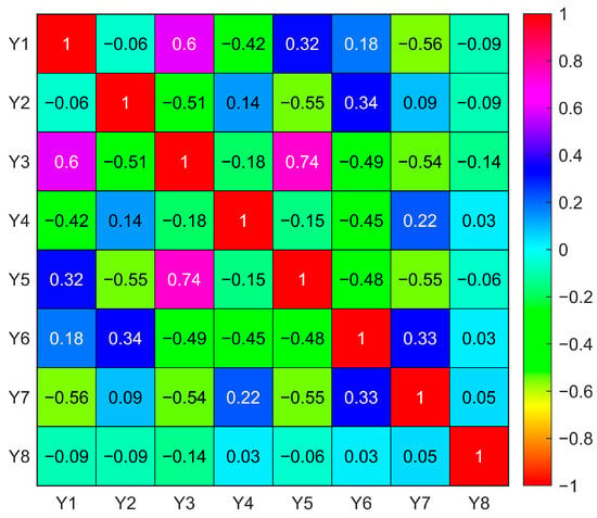
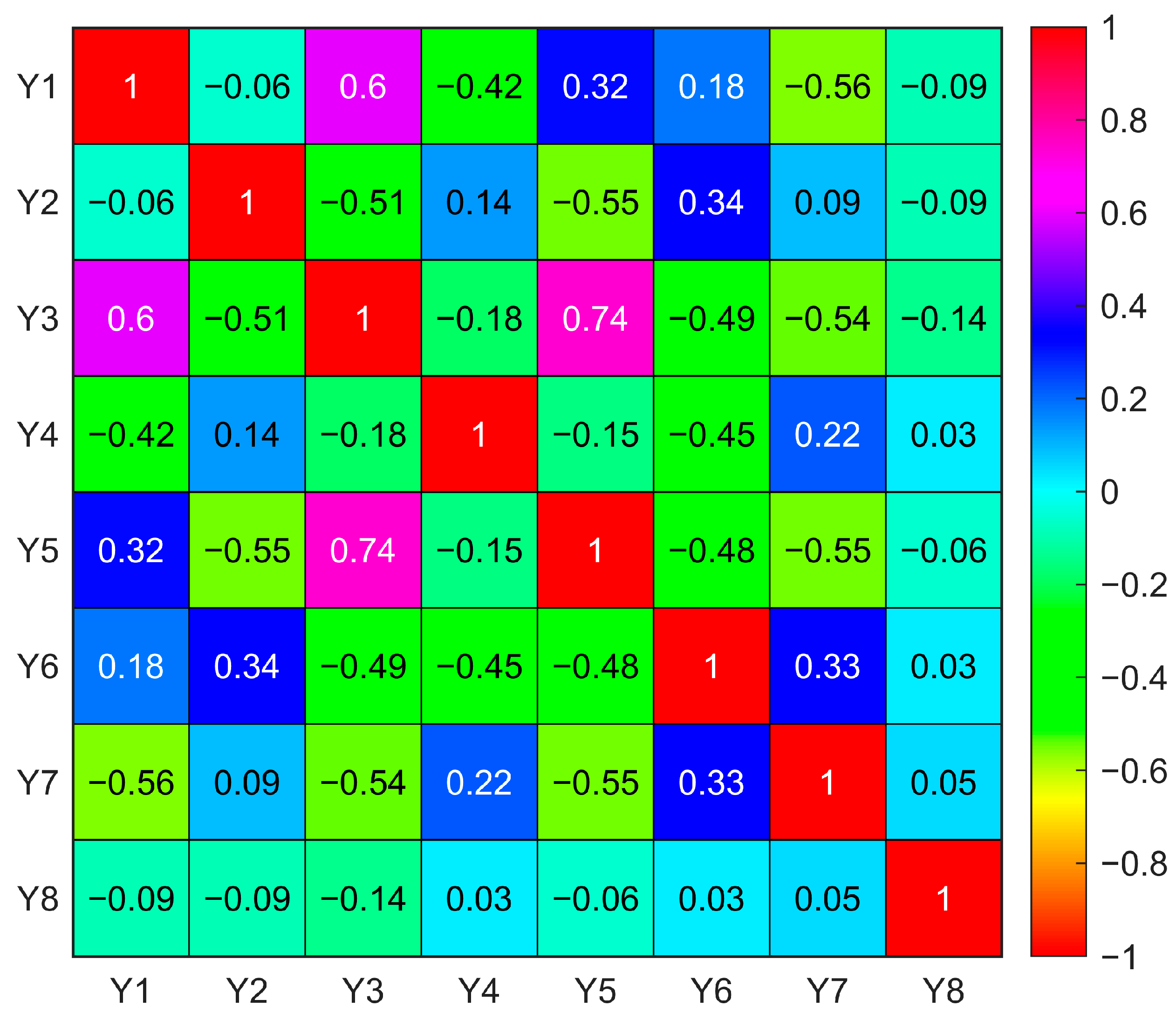
The Pearson correlation coefficients between input parameters were calculated, and the results are shown in Figure 1. All absolute values of the correlation coefficients are less than 0.80, indicating no strong linear correlation among the input parameters. Thus, the mutual interference among these parameters exerts a negligible effect on the prediction of RAC creep behavior.

Figure 1. Pearson correlation coefficients between input parameters.

2.3. Database Processing

Before machine learning modeling, direct model training without data preprocessing may degrade training stability and convergence efficiency, owing to the large differences in dimensions and value ranges among input and output parameters. Therefore, all parameters were normalized to unify data scales and accelerate model convergence [45]. It should be noted that the normalization parameters were calculated only based on the training set. The same normalization parameters obtained from the training set were then applied to transform the test set, thereby avoiding potential data leakage and ensuring an unbiased evaluation of the model performance. The corresponding normalization formula is presented in Equation (2). Since the models were trained on the basis of normalized data, the predicted results require scale restoration via inverse transformation. The formula for inverse normalization is illustrated in Equation (3).

$$Y_{\mathrm{norm}}={\displaystyle \frac{Y-Y_{\min }}{Y_{\max }-Y_{\min }}}$$

(2)

Y_r = Y_norm × (Y_max − Y_min) + Y_min

(3)

where Y is the raw data before normalization, Y_min and Y_max are the minimum and maximum values of each variable, respectively, and Y_r denotes the denormalized data.

In addition, for the gene expression programming (GEP) model, the data were scaled to values between 0.1 and 1. The function set adopted for fitness calculation involves division operations. If the data are normalized to the range of [0, 1], the denominator may approach zero and produce abnormal values, thereby affecting model stability. The corresponding normalization and inverse normalization formulas are presented in Equations (4) and (5), respectively.

$$Y_{\mathrm{norm}}=0.9\times {\displaystyle \frac{Y-Y_{\min }}{Y_{\max }-Y_{\min }}}+0.1$$

(4)

$$Y_r={\displaystyle \frac{Y_{\mathrm{norm}}-0.1}{0.9}}\times (Y_{\max }-Y_{\min })+Y_{\min }$$

(5)

2.4. Evaluation Metrics

In this study, four commonly used statistical evaluation metrics were adopted for model performance assessment, including the coefficient of determination (R²), mean absolute error (MAE), root mean square error (RMSE). The calculation formulas for these metrics are presented in Equations (6)–(9).

$${\mathrm{R}}^2=1-{\displaystyle \frac{{\displaystyle \sum _{x=1}^n{(y_x-{y^{\prime }}_x)}^2}}{{\displaystyle \sum _{x=1}^n{(y_x-\overline{y})}^2}}}$$

(6)

$$\mathrm{MAE}={\displaystyle \frac{1}{n}}{\displaystyle \sum _{x=1}^n|}{y}_x-{y^{\prime }}_x|$$

(7)

$$\mathrm{RMSE}=\sqrt{{\displaystyle \frac{1}{n}}{\displaystyle \sum _{x=1}^n{(y_x-{y^{\prime }}_x)}^2}}$$

(8)

$$\mathrm{MAPE}={\displaystyle \frac{1}{n}}{\displaystyle \sum _{x=1}^n\left|\frac{y_x-{y^{\prime }}_x}{y_x}\right|}$$

(9)

Among the above evaluation metrics, the coefficient of determination R² is one of the most widely utilized indicators for model evaluation, which mainly measures the fitting degree of the model to the variation characteristics of measured data. A higher R² value indicates better model fitting performance. MAE reflects the average deviation of the predicted values from their corresponding measured values. RMSE quantifies the overall prediction error and is more sensitive to large errors, and therefore can more effectively characterize the response of the model to abnormal deviations. MAPE is adopted to quantify the relative deviation of predicted results from measured values. In general, for concrete creep prediction, a larger R² and smaller MAE, RMSE, and MAPE indicate better prediction performance of the model.

3. Machine Learning Models

3.1. Back-Propagation Neural Network (BPNN)

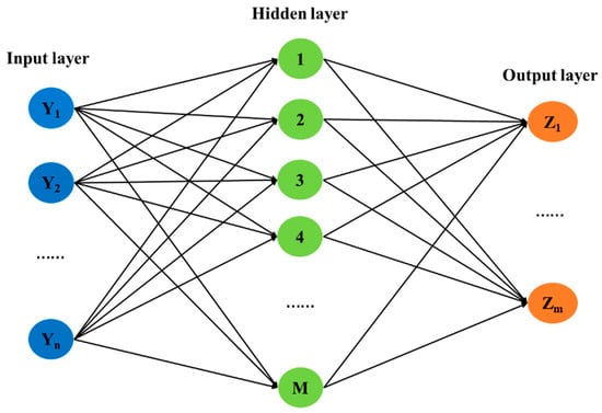
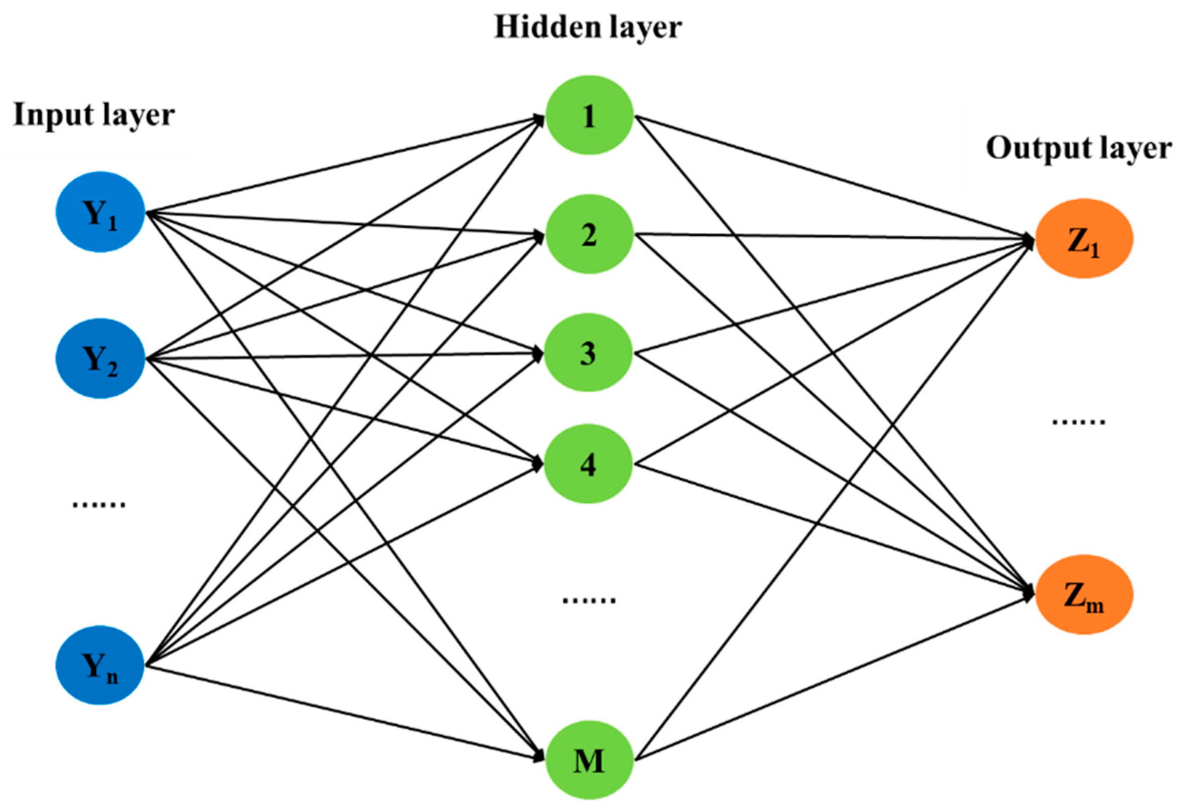
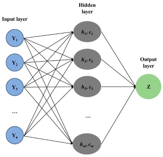
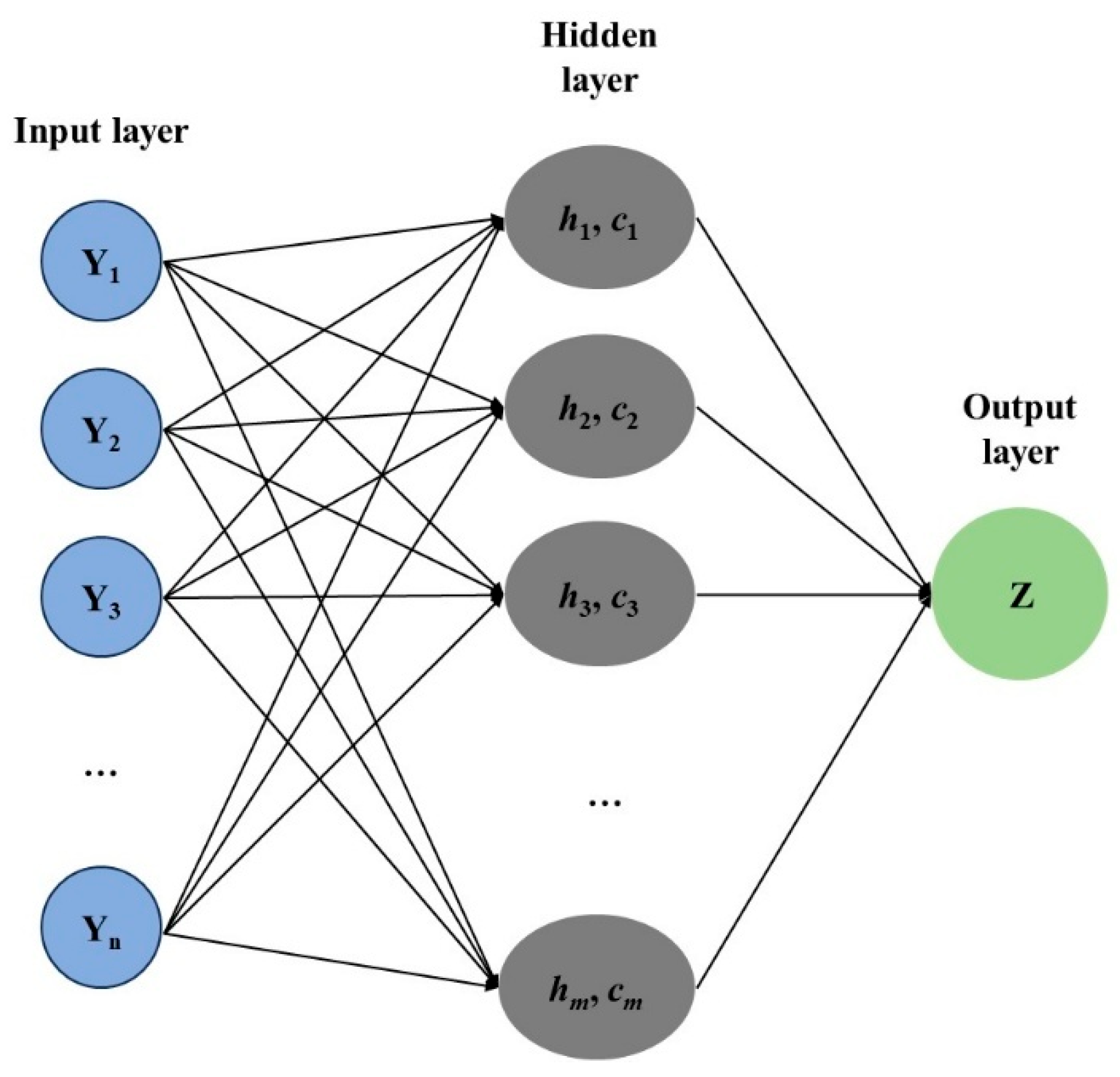
The topological structure of the BPNN is illustrated in Figure 2. The training process of the BPNN consists of two stages. In the forward propagation stage, the training samples are transmitted from the input layer to the output layer through the hidden layer, and the activation values are calculated to obtain the output results, which are then compared with the expected values. If the error satisfies the required criterion, the training process is terminated, otherwise, the back-propagation stage is performed. In the back-propagation stage, the error signal is propagated backward, and the connection weights and bias parameters of each layer are adjusted layer by layer until the network error converges to the minimum value.

Figure 2. Structure of BPNN.

The BPNN model was trained using the trainlm function. This function adjusts network weights and thresholds based on the Levenberg–Marquardt algorithm [46] to minimize the overall training error. A single-hidden-layer network structure was adopted, with one input layer, one hidden layer, and one output layer. For the selection of transfer functions, the transfer function from the input layer to the hidden layer was set as tansig, while a linear transfer function was adopted from the hidden layer to the output layer, so as to ensure that the output range was not restricted and that the model was more suitable for continuous variable prediction.

Currently, no unified criterion is available for determining the optimal number of hidden-layer neurons. In engineering practice, empirical formulas are widely utilized to estimate the feasible range of neuron quantity. The empirical formulas employed in this study are presented in Equations (10)–(12). In these equations, M denotes the number of neurons in the hidden layer, k represents the total number of samples in the database, n refers to the number of input parameters, m indicates the number of nodes in the output layer, and c is a constant ranging from 0 to 10.

$${\displaystyle \sum _{i=0}^n{C}_M^i}>k$$

(10)

$$M=\sqrt{n+m+c}$$

(11)

M = log₂n

(12)

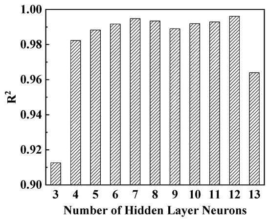
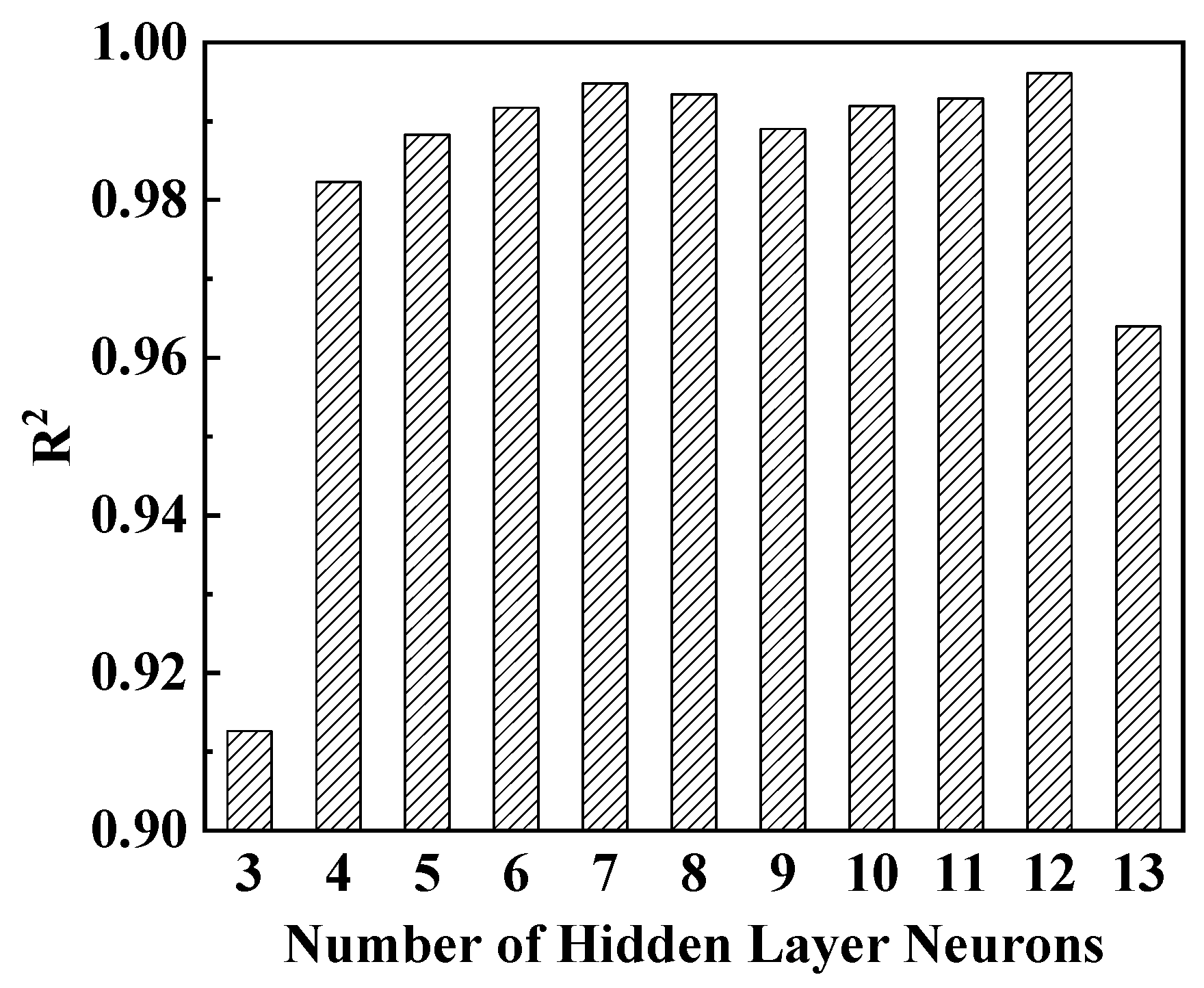
Based on the above empirical formulas, the candidate range of hidden-layer neurons was determined to be [3,13]. To identify the optimal node number, this study adopted the R² as the model evaluation metric and established a series of BPNN models with hidden-layer neurons ranging from 3 to 13. The corresponding R² values of different models were calculated, with the comparative results presented in Figure 3. The results show that the maximum R² value is achieved when the number of hidden-layer neurons is 12. Accordingly, the hyperparameter configuration of the BPNN model was finalized, as listed in Table 2.

Figure 3. Relationship between R² and the number of hidden layer neurons.

Table 2. Hyperparameter configuration of BPNN model.

Hyperparameters	Configuration
Number of input neurons	8
Number of hidden layer neurons	12
Number of output neurons	1
Optimization algorithm	Levenberg–Marquardt
Transfer functions	Tansig, Purelin
Maximum training epochs	1000
Goal error	10−5
Learning rate	0.01

3.2. Radial Basis Function Neural Network (RBFNN)

The structure of the RBFNN is illustrated in Figure 4. The input layer directly passes the original database data, while hidden-layer nodes generate nonlinear responses through distance calculations between the inputs and the center points. During model establishment, the parameters of the basis functions should be reasonably determined, and the number of nodes should be controlled to avoid overfitting.

Figure 4. Structure of RBFNN.

The Gaussian function was adopted as the radial basis function for RBFNN modeling. The output of the RBFNN was obtained through a weighted function, and the weights were calculated using the linear least squares method. The Gaussian function and the least squares method are expressed in Equations (13) and (14), respectively.

$$h_j(y)=\exp \left(-{\displaystyle \frac{\Vert y-c_j{\Vert }^2}{2{\sigma }_j^2}}\right)$$

(13)

$$Z={\displaystyle \sum _{j=1}^m{w}_j}{h}_j(y)$$

(14)

where y is the input sample vector, ‖∙‖ denotes the Euclidean distance, h_j is the output value of the j-th hidden layer neuron, c_j and ${\sigma }_j^2$ are the center vector and width parameter (spread parameter) of the j-th hidden layer neuron, respectively, m is the number of hidden layer neurons, and w_j is the connection weight from the j-th hidden layer neuron to the output layer.

Through multiple trials based on the training set, this study determined a spread value of 15 for the RBFNN model, which provided satisfactory fitting performance during model training. In addition, the hidden layer was configured with 280 neurons. The hyperparameter configuration was determined using only the training set while the test set was not involved in model optimization and was exclusively used for the final evaluation of prediction performance. The final hyperparameter configuration of the RBFNN model is summarized in Table 3.

Table 3. Hyperparameter configuration of RBFNN model.

Hyperparameters	Configuration
Number of input neurons	8
Number of hidden layer neurons	280
Number of output neurons	1
Spread constant	15
Radial basis function	Gaussian function

3.3. Support Vector Regression (SVR)

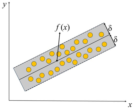
The structural diagram of the SVR model is presented in Figure 5. The yellow circles denote sample data points. SVR modeling was implemented using the LIBSVM-3.22 toolbox developed by Chih-Jen Lin at National Taiwan University. The radial basis function (Gaussian kernel) was adopted as the kernel function in this study. The specific objective function of SVR is presented in Equation (15), which balances model complexity and training error.

$$\min {\displaystyle \frac{1}{2}}\Vert w{\Vert }^2+C{\displaystyle \sum _{i=1}^n\left({\xi }_i+{\xi }_i^{*}\right)}$$

(15)

where ‖w‖² is the weight vector, C is the regularization parameter that balances the trade-off between error and margin size, ξ_i and ${\xi }_i^{*}$ are slack variables representing the deviation of each data point, and n denotes the total number of samples used for model training.

Figure 5. SVR model.

The kernel function calculates the similarity between input parameters and training data points, which maps the original database data into a high-dimensional feature space to achieve nonlinear transformation. The final regression model is established by integrating support vectors and the kernel function, as illustrated in Equation (16).

$$f(x)={\displaystyle \sum _{i=1}^n\left({\alpha }_i-{\alpha }_i^{*}\right)}K(x_i,x_j)+b$$

(16)

where α_i and ${\alpha }_i^{*}$ are the introduced Lagrange multipliers, and the bias term b is calculated using the support vectors.

The hyperparameters of the SVR model include the kernel function parameter (g), tolerance error p (i.e., ε), and penalty factor c. Through multiple trial tests, the values of p, c, and g were finally set to 0.05, 15, and 1.6, respectively, to achieve optimal regression performance. The detailed hyperparameter configuration of the SVR model is summarized in Table 4.

Table 4. Hyperparameter configuration of SVR model.

Hyperparameters	Configuration
Kernel function	Gaussian function
p	0.05
c	15
g	1.6

3.4. Random Forest (RF)

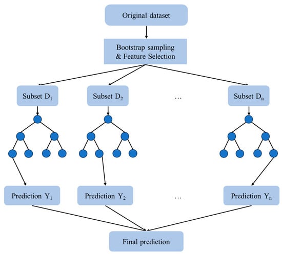
The structural framework of the RF model is illustrated in Figure 6. Each decision tree is trained independently, and the training dataset for individual trees is generated via bootstrap sampling (i.e., sampling with replacement). During node splitting, each tree randomly selects a subset of features for optimal segmentation, thereby improving inter-tree diversity. A single decision tree is susceptible to overfitting. By contrast, the RF algorithm greatly reduces the overall model variance by decreasing the correlation between trees while maintaining a low bias level. By averaging the prediction outputs of multiple base trees, the RF model effectively mitigates model overfitting to the training database data.

Figure 6. Structure of RF model.

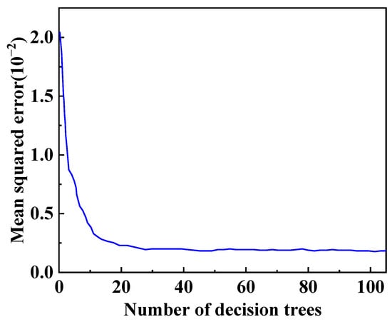
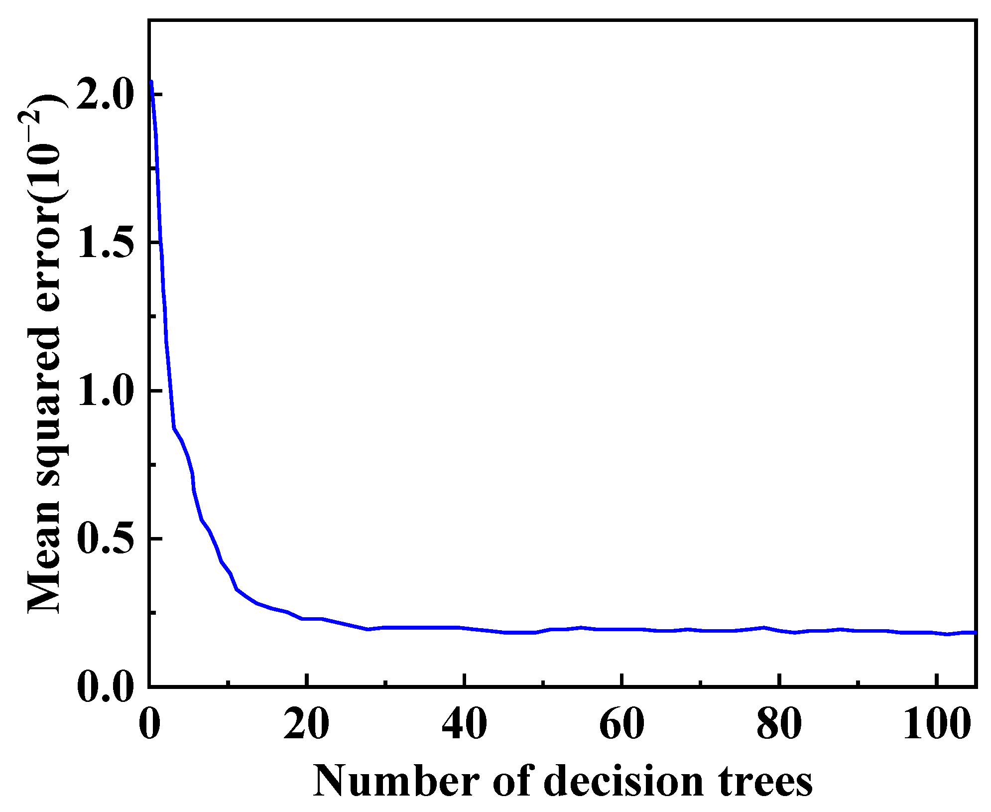
When establishing the RF model for RAC creep prediction, the number of decision trees was set to 105 and the minimum number of samples per leaf node was set to 1 based on the database scale and multiple trial tests. The out-of-bag error was adopted to monitor model performance during RF modeling. Given that the training database contained 280 samples, each decision tree was generated through 280 rounds of random sampling with replacement, allowing individual samples to be selected repeatedly. Approximately 63.2% of the total samples were selected at least once for tree training, while the remaining 36.8% of samples, namely out-of-bag samples, were excluded from training and utilized for model validation. The detailed hyperparameter configuration of the RF model is summarized in Table 5.

Table 5. Hyperparameter configuration of RF model.

Hyperparameters	Configuration
Number of decision trees	105
Minimum number of samples at leaf nodes	1
Total number of samples	280
Sampling strategy	Random sampling with replacement

For each out-of-bag sample, predictions were generated exclusively by decision trees that exclude the corresponding sample during training, and the final prediction was determined by averaging these individual outputs. The variation in MSE for different decision trees was calculated and presented in Figure 7. The results revealed that the MSE decreased rapidly at first and then gradually stabilized as the number of decision trees rose. Specifically, the MSE dropped sharply with the increase in tree number when the value was less than 8. For tree numbers between 8 and 28, the declining rate of MSE gradually slowed down. When the tree number exceeded 28, the MSE converged steadily with negligible further reduction and eventually remained stable.

Figure 7. MSE of different decision trees.

3.5. Gene Expression Programming (GEP)

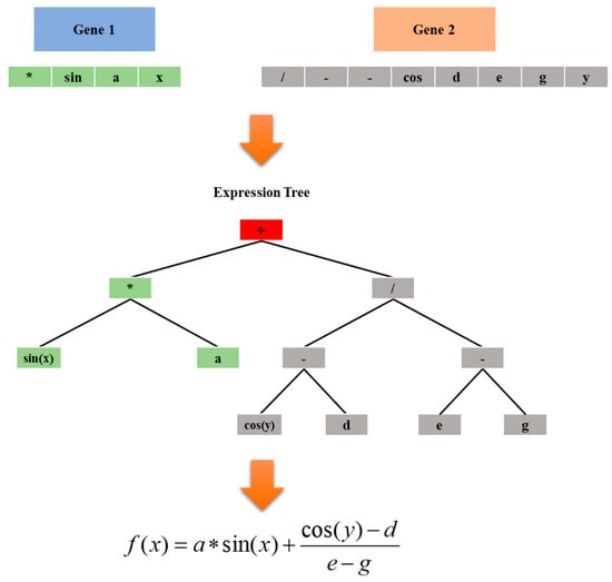
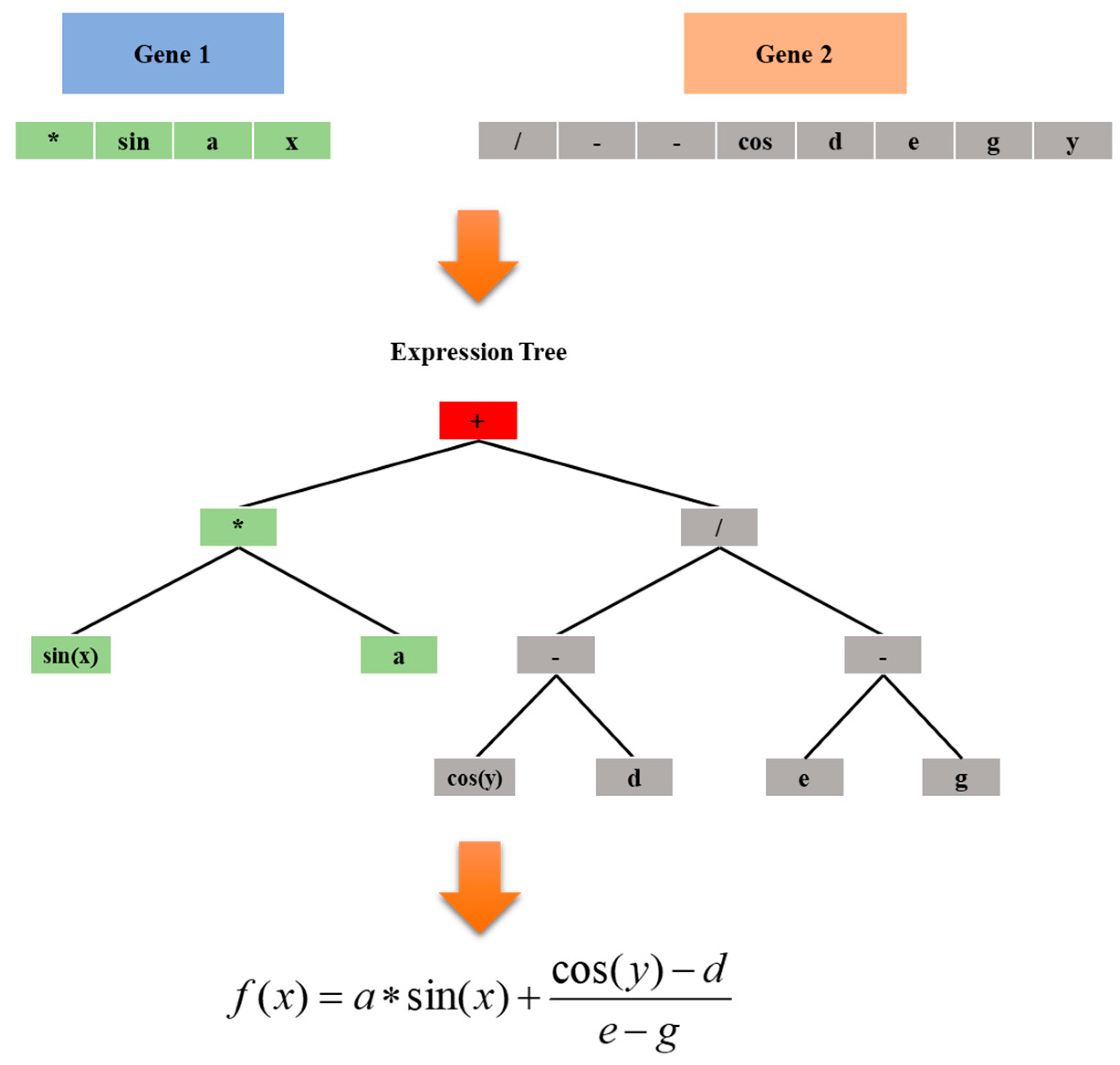
GEP is an evolutionary computation technique that integrates the advantages of genetic algorithms and genetic programming. It combines the fixed-length linear coding of genetic algorithms with the tree-like topological structure of genetic programming, enabling efficient solutions to complex problems through concise coding rules. Its computational speed is two to four orders of magnitude faster than that of traditional algorithms. Reasonable selection of core parameters, including population size, gene length, recombination rate, mutation rate, and genetic operators, is essential for GEP modeling. The basic implementation flow of the GEP is illustrated in Figure 8.

Figure 8. Basic process of the GEP.

The hyperparameters of the GEP model applied in this study were set as follows: the population size was 1000, the gene length was 25, and the number of genes was 3. The function set covered addition, subtraction, multiplication, division, sine, cosine, and exponential functions, among which addition was adopted as the gene linking function. Both the one-point and two-point recombination rates were set to 0.45, and the maximum number of iterations was set to 8000. Tournament selection was utilized as the selection strategy. In each selection iteration, three chromosomes were randomly selected for competitive screening, and the chromosome with the highest fitness was chosen as the parent individual. This strategy is simple to implement and facilitates the efficient screening of dominant individuals. A piecewise increasing strategy was adopted for the mutation rate: the mutation rate was 0.025 for iterations below 1000, 0.05 for 1000–2000 iterations, 0.10 for 2000–4000 iterations, and 0.20 for iterations exceeding 4000. Meanwhile, the mechanisms of elitism preservation and random individual insertion were introduced in the model evolution. The top 5% of superior individuals were directly inherited to the next generation to avoid the degradation of high-quality solutions, and approximately 10% of new chromosomes were randomly generated to enrich population diversity. The remaining individuals were produced through tournament selection, one-point recombination, two-point recombination, and mutation operations. The R² was selected as the fitness function. The complete hyperparameter configuration of the GEP model is summarized in Table 6.

Table 6. Hyperparameter configuration of GEP model.

Hyperparameters	Configuration
Population size	1000
Gene length	25
Number of genes	3
Function set	Addition, subtraction, multiplication, division, sine, cosine and exponential functions
One-point recombination rate and two-point recombination rate	0.45
Maximum number of iterations	8000
Selection strategy	Tournament selection
Mutation rate (a)	Iterations < 2000, a = 0.025, 1000 < iterations < 2000, a = 0.05, 2000 < iterations < 4000, a = 0.10, 4000 < iterations, a = 0.2
Population mechanism	Elitist preservation strategy and random new individual insertion
Fitness function	R2

With the above hyperparameter settings, the GEP model was constructed to obtain the explicit functional relationships between input and output parameters. The corresponding expressions are presented in Equations (17)–(22).

Z = Z₁ + Z₃ + Z₅

(17)

Z₁ = Y₈sin(Y₃(Y₇ − Y₈ + exp(Y₂) + Z₂))

(18)

$$Z_2={\displaystyle \frac{Y_4{Y}_7}{Y_8\sin (\cos (Y_1))\sin (\exp (Y_1))}}$$

(19)

$$Z_3=\sin \left({\displaystyle \frac{Y_7\sin (Y_5)}{Z_4}}\right)$$

(20)

$$Z_4=Y_1\left(Y_6-\exp \left({\displaystyle \frac{Y_6\sin (\cos (Y_1))(Y_7+\sin (Y_5))}{Y_1}}\right)\right)$$

(21)

Z₅ = Y₂Y₃

(22)

4. Model Performance and Result Comparison

4.1. BPNN

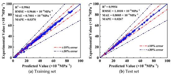
Figure 9 presents the predictive results obtained by the BPNN model for the training and test sets. All predicted values mostly lie within the ±10% error range. The R² values of the BPNN model on both the training and test sets exceed 0.99, demonstrating outstanding predictive capability and approaching the theoretical optimal value of 1. The test-set R² is only 0.07% lower than its training-set counterpart, indicating that the patterns learned from the training set can be effectively transferred to unseen data. The model maintains high adaptability to new data, and no overfitting is observed.

Figure 9. Predictive performance of the BPNN model for the training and test sets.

The difference between RMSE and MAE is 0.2645 × 10⁻⁶ MPa⁻¹ for the training set and 0.3013 × 10⁻⁶ MPa⁻¹ for the test set. The small discrepancies reveal that prediction errors are distributed relatively evenly and are barely affected by extreme outliers. This result verifies that the model possesses excellent robustness and can tolerate data noise and distribution fluctuations in practical engineering applications. The MAPE values for the training and test sets are 0.0370 and 0.0267, respectively. Both values are low, and their gap is negligible, which further validates the high prediction accuracy of the BPNN model.

4.2. RBFNN

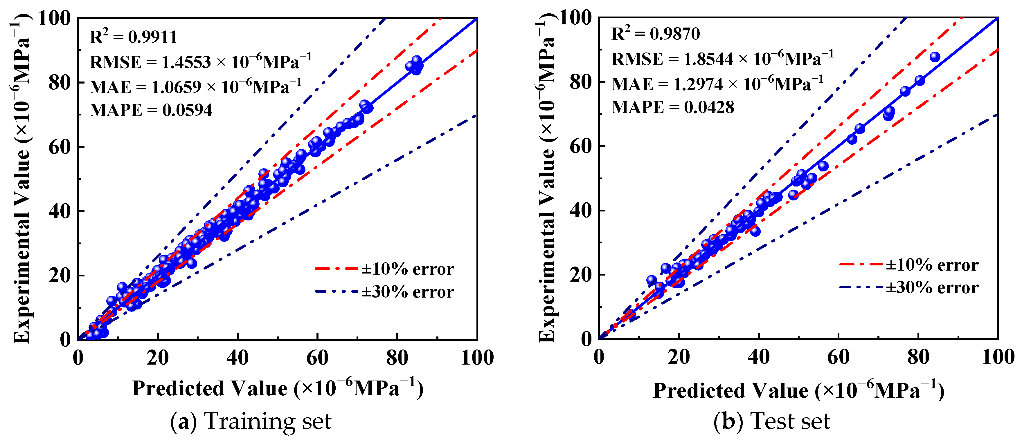
Figure 10 illustrates the predictive performance of the RBFNN model for the training and test sets. All predicted values mostly lie within the ±10% error range and show good consistency with the measured values. The R² of the model on both the training and test sets exceeds 0.95, indicating that the model achieves excellent fitting accuracy and predictive capability. Meanwhile, the R² of the test set decreases by only about 0.41% relative to the training set, indicating that no obvious overfitting occurs during model training. The feature relationships learned by the model can be stably applied to unseen samples, and the model exhibits strong generalization capability for new data.

Figure 10. Predictive performance of the RBFNN model for the training and test sets.

As observed from the training and test results in Figure 10, the differences between RMSE and MAE are 0.3894 × 10⁻⁶ MPa⁻¹ for the training set and 0.557 × 10⁻⁶ MPa⁻¹ for the test set. The small discrepancies indicate that the prediction errors of the model are relatively uniformly distributed, and no large number of extreme prediction errors occurs in either the training or test set. The error distribution is relatively concentrated, and the model has low sensitivity to outliers, which further verifies its stability. The training-set and test-set MAPE values are 0.0594 and 0.0428, respectively. Their consistently low magnitudes further confirm the high accuracy of the RBFNN.

4.3. SVR

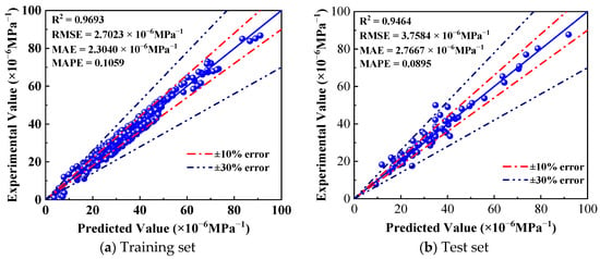
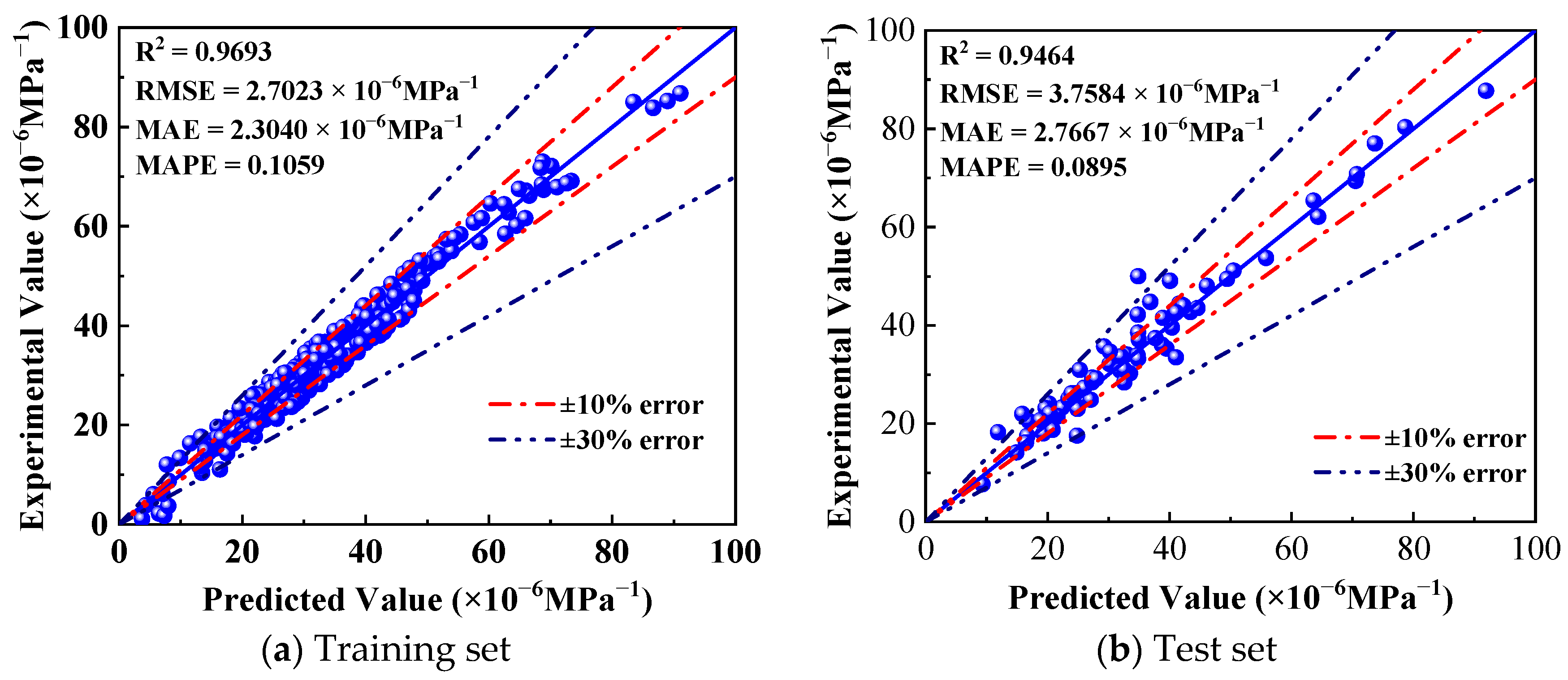
Figure 11 illustrates the predictive results of the SVR model for the training and test sets. Most predicted values fall within the ±10% error range, while a small number of predicted values are distributed within or near the ±30% error range. The R², RMSE, and MAE values of the SVR model on the training and test sets are relatively close, indicating that no overfitting occurs in the SVR model. The R² of the test set decreases by 2.36% compared with that of the training set. This reveals that the model’s ability to capture inherent data patterns declines slightly, yet it still retains strong predictive capability. The RMSE of the test set increases by 39.1% compared with that of the training set, and the MAE increases by 20.1%, suggesting a modest decline in model performance on unseen data, although the deterioration remains limited. The MAPE values for the training and test sets are 0.1059 and 0.0895, respectively. Both values stay at low levels, which further confirms the excellent prediction accuracy of the SVR model.

Figure 11. Predictive performance of the SVR model for the training and test sets.

As observed from the results in Figure 11, the differences between RMSE and MAE are 0.3983 × 10⁻⁶ MPa⁻¹ for the training set and 0.9913 × 10⁻⁶ MPa⁻¹ for the test set. These minor discrepancies indicate that prediction errors are distributed relatively evenly, and no obvious extreme errors emerge during training or testing. The error distribution is concentrated overall, and the model shows low sensitivity to outliers, which further verifies its stability.

4.4. RF

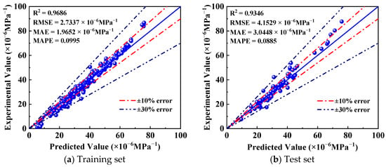
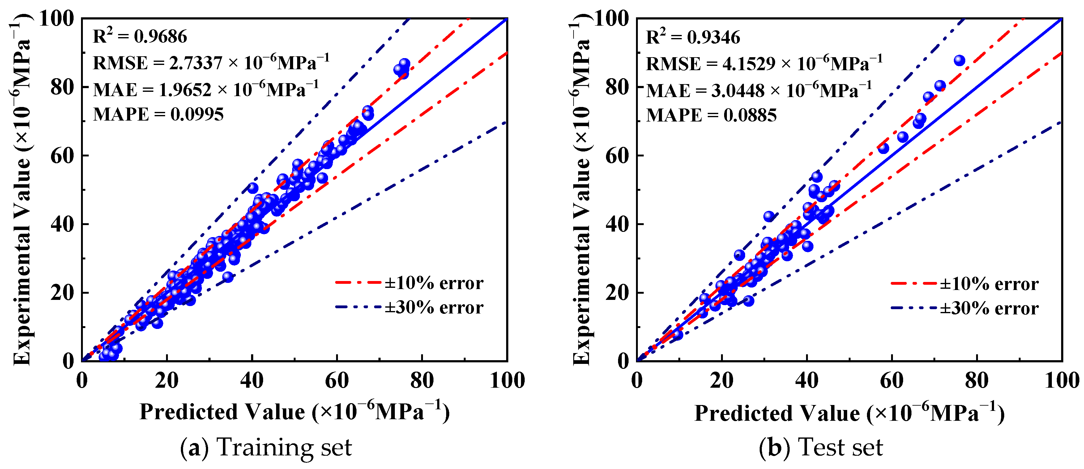
Figure 12 presents the prediction performance of the RF model on the training and test sets. Most predicted values fall within the ±10% error range, while a small number of predicted values are distributed within or near the ±30% error range. For the training set, the R², RMSE, MAE, and MAPE values of 0.9686, 2.7337 × 10⁻⁶ MPa⁻¹, 1.9652 × 10⁻⁶ MPa⁻¹, and 0.0995 on the training set, respectively, indicating that the model achieves excellent accuracy on training samples. The model can explain 96.86% of the variance in the training data with relatively low prediction errors. This result verifies the strong fitting capability of RF for the training data through ensemble learning and input parameter importance screening.

Figure 12. Predictive performance of the RF model for the training and test sets.

For the test set, the R², RMSE, MAE, and MAPE of the RF model are 0.9346, 4.1529 × 10⁻⁶ MPa⁻¹, 3.0448 × 10⁻⁶ MPa⁻¹, and 0.0885, respectively, confirming that the model retains excellent prediction accuracy on unseen data. Compared with the training set, the R² value of the test set decreases merely only 3.51%, a relatively slight reduction that reveals the strong generalization ability of the model and the absence of evident overfitting. Meanwhile, the MAE, RMSE, and MAPE values of the test set remain at relatively low levels, and without order-of-magnitude error differences between the training and test sets, proving that the model does not generate excessive dependence on training data.

4.5. GEP

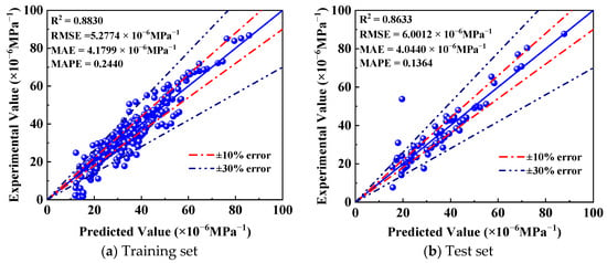
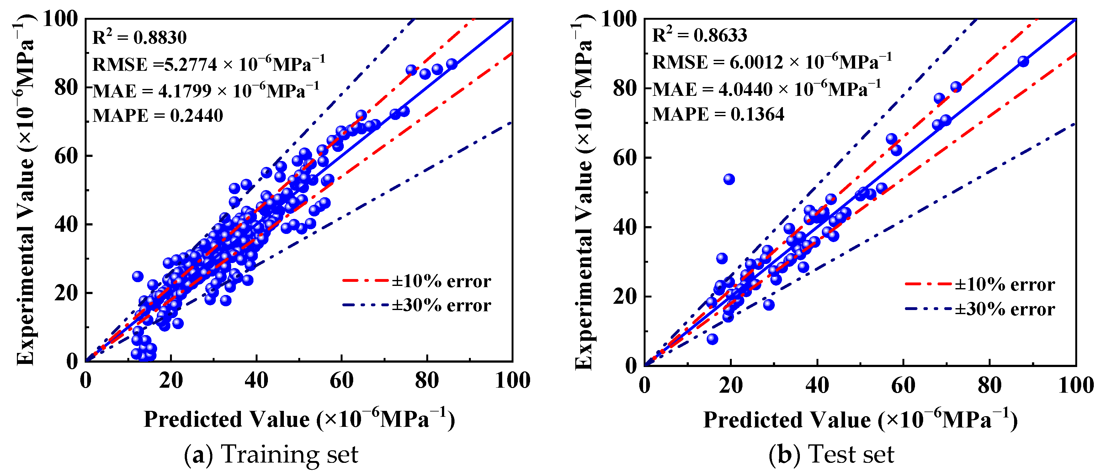
Figure 13 presents the prediction performance of the GEP model on the training and test datasets, where the majority of predicted values lie within the ±30% error range. The results show that the R² of the training set is 0.8830, indicating that the model can explain 88.30% of the variance in the training data. The R² of the test set is 0.8633, which decreases by only 2.23% compared with that of the training set. The RMSE values of the training and test sets are 5.2774 × 10⁻⁶ MPa⁻¹ and 6.0012 × 10⁻⁶ MPa⁻¹, respectively, which are of a similar order of magnitude and relatively low, suggesting that the model yields only small prediction deviations for the output parameter.

Figure 13. Predictive performance of the GEP model for the training and test sets.

The MAPE values of the training and test sets are 0.2440 and 0.1364, respectively, and the MAE values of the training and test sets are 4.1799 × 10⁻⁶ MPa⁻¹ and 4.0440 × 10⁻⁶ MPa⁻¹, respectively. A slight abnormal trend is observed, in which the test set exhibits lower MAE and MAPE values than the training set. This may be attributed to the lower proportion of extreme values or noise in the test set, as well as the possibility that the data split inadvertently assigned samples with relatively lower prediction difficulty to the test set. Overall, the R² values of the GEP model for both datasets exceed 0.85, which verifies the reliable predictive capability of the proposed model.

4.6. Comparison of Machine Learning Models

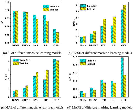
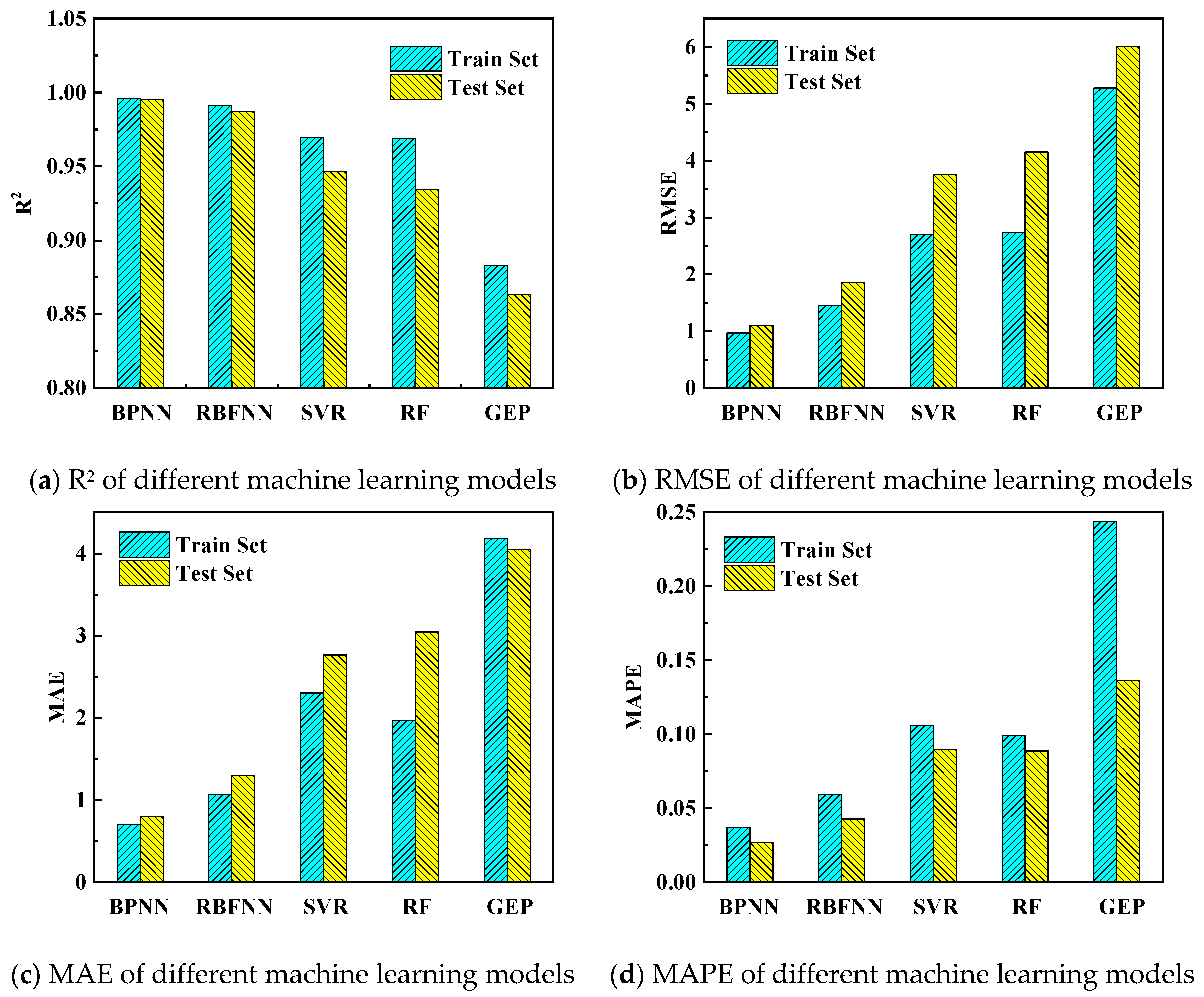
Four quantitative evaluation metrics were adopted to evaluate and compare the predictive performance of all machine learning models, so as to screen out the optimal model. Figure 14 presents the comprehensive comparison of the four metrics across different models, which intuitively reflects the differences in predictive performance among the constructed machine learning algorithms.

Figure 14. Four evaluation metrics of different machine learning models.

Figure 14a compares the R² values obtained by the five machine learning models for both the training and test sets. For the training set, the R² values decrease in the order BPNN > RBFNN > SVR > RF > GEP, demonstrating that the BPNN model achieves the optimal fitting performance in the training phase. Similarly, the test-set R² maintains the same ranking order, indicating that BPNN also exhibits the best predictive performance for model validation. The R² differences between the training and test sets for BPNN, RBFNN, SVR, RF, and GEP are 0.0007, 0.0041, 0.0229, 0.0340, and 0.0197, respectively. BPNN presents the minimum R² difference, followed by RBFNN. For machine learning models with high accuracy on both training and test sets, a smaller R² discrepancy indicates more consistent performance and better generalization and stability. Considering the R² values of the machine learning models on both the training and test sets, the BPNN model provides the best prediction performance for RAC creep, followed by RBFNN.

Figure 14b compares the RMSE values obtained by the five machine learning models for both the training and test sets. For the training set, the RMSE values increase in the order BPNN < RBFNN < SVR < RF < GEP, demonstrating that the BPNN model yields the minimum prediction error in the training phase. Similarly, the test-set RMSE maintains the same ranking order, indicating that BPNN also achieves the lowest prediction error during model validation. Considering the RMSE values of the machine learning models on both the training and test sets, the BPNN model has the smallest error in predicting RAC creep, followed by RBFNN.

Figure 14c compares the MAE values obtained by the five machine learning models for both the training and test sets. For the training set, the MAE values increase in the order BPNN < RBFNN < RF < SVR < GEP, demonstrating that the BPNN model yields the minimum prediction error in the training phase, with RBFNN ranking second. The test-set MAE follows a slightly different ranking of BPNN < RBFNN < SVR < RF < GEP, indicating that BPNN still achieves the lowest prediction error during model validation, followed by RBFNN. Considering the MAE values of the machine learning models on both the training and test sets, the BPNN model has the smallest error in predicting RAC creep, followed by RBFNN.

Figure 14d compares the MAPE values obtained by the five machine learning models for both the training and test sets. For the training set, the MAPE values increase in the order BPNN < RBFNN < RF < SVR < GEP, demonstrating that the BPNN model yields the minimum prediction error in the training phase, with RBFNN ranking second. Similarly, the test-set MAPE maintains the identical ranking order, indicating that BPNN also achieves the lowest MAPE during model validation, followed by RBFNN. Considering the MAPE values of the machine learning models on both the training and test sets, BPNN has the smallest MAPE, followed by RBFNN.

In summary, based on the four evaluation metrics of the five machine learning models on both training and test sets, the BPNN model delivers the optimal prediction accuracy, with RBFNN ranking second. This result indicates that the BPNN and RBFNN models are more applicable and reliable for predicting the creep performance of recycled aggregate concrete.

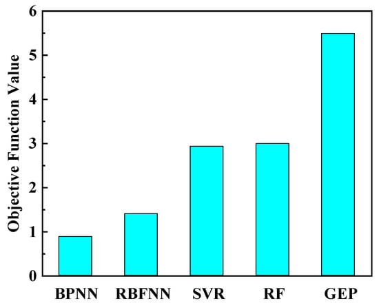
To further quantitatively analyze the advantages and disadvantages of each model, an objective function was adopted to evaluate each model, as shown in Equation (23). In this equation, N is the total number of samples in the dataset, N₁ is the number of samples in the training set, and N₂ is the number of samples in the test set. ${\mathrm{R}}_1^2$ and ${\mathrm{R}}_2^2$ are the R² values of the training and test sets, respectively, RMSE₁ and RMSE₂ are the RMSE values of the training and test sets, respectively, and MAE₁ and MAE₂ are the MAE values of the training and test sets, respectively. A smaller value of y indicates higher model accuracy, whereas a larger value indicates lower model accuracy.

$$y={\displaystyle \frac{N_1-N_2}{N}}\ast {\displaystyle \frac{{\mathrm{RMSE}}_1+{\mathrm{MAE}}_1}{{\mathrm{R}}_1^2+1}}+{\displaystyle \frac{2N_2}{N}}\ast {\displaystyle \frac{{\mathrm{RMSE}}_2+{\mathrm{MAE}}_2}{{\mathrm{R}}_2^2+1}}$$

(23)

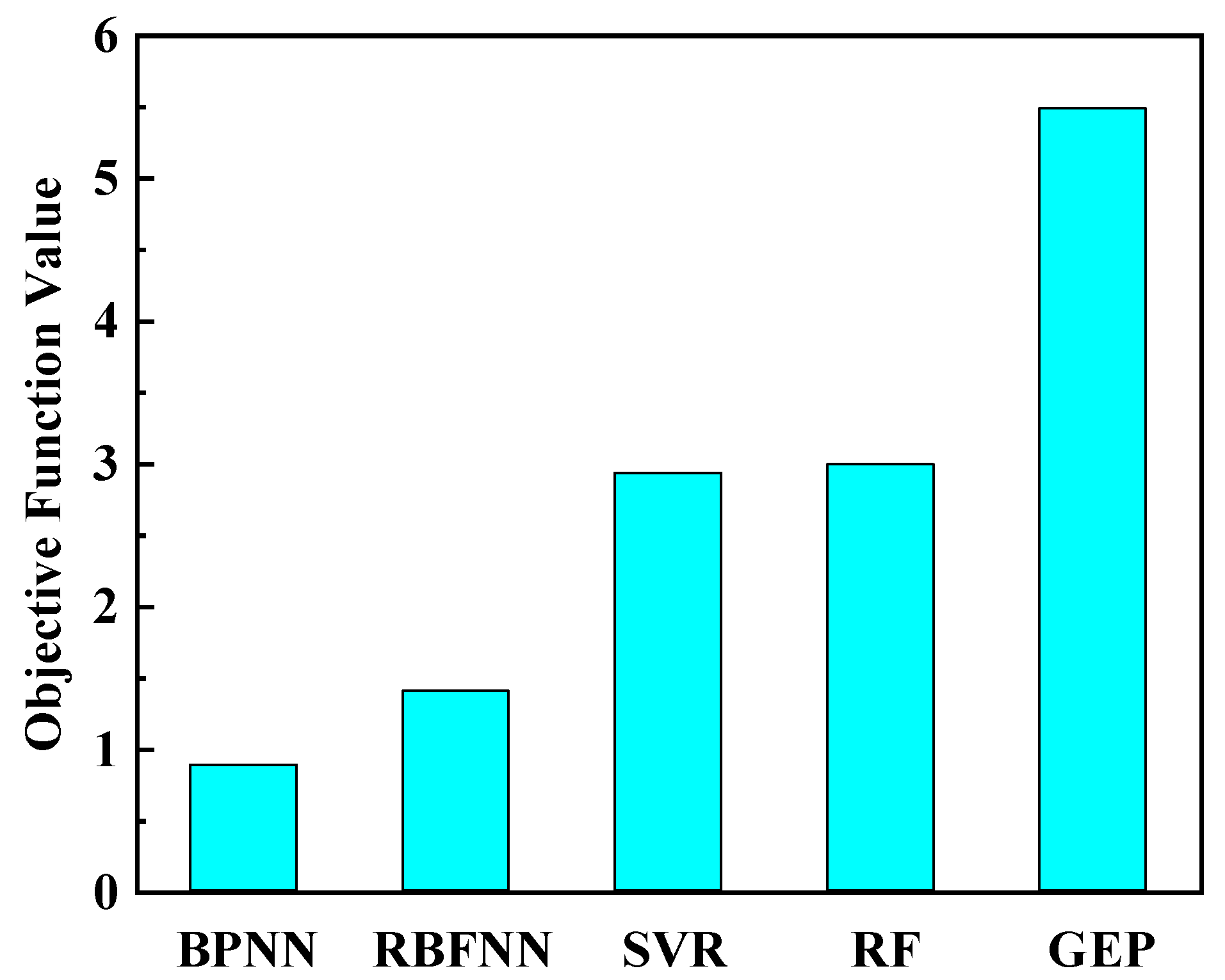
Figure 15 illustrates the variation in the objective function values of the five machine learning models. As observed from the figure, the BPNN model achieves the minimum objective function value of 0.88, which corresponds to the optimal prediction accuracy among all models. The remaining models follow the performance ranking of RBFNN, SVR, RF, and GEP in sequence.

Figure 15. Calculated values of the objective function for machine learning models.

4.7. Model Application

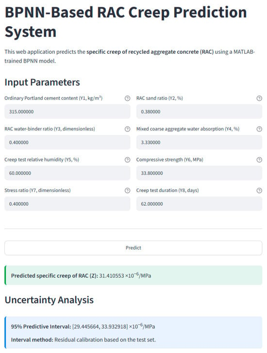
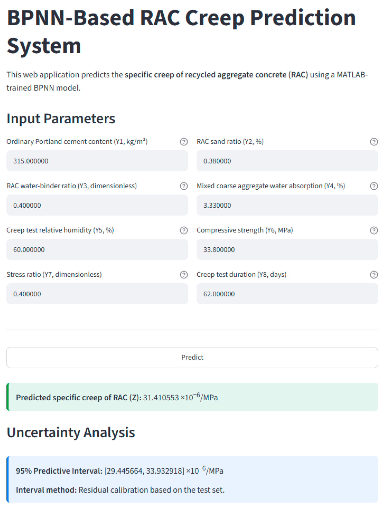
To facilitate the application of the established BPNN creep prediction model, this study developed an RAC specific creep prediction system based on the well-trained BPNN model within the scope of this study. The system was constructed as a web-based graphical user interface (GUI) using Python 3.9.7 and the Streamlit framework, realizing the effective conversion of the BPNN model from the MATLAB R2022b training environment to the Python 3.9.7 web application environment. During system development, the BPNN model was first trained in MATLAB R2022b, and the core model information, including network weights, thresholds, activation functions, and input–output normalization parameters, was saved. These parameters were then exported to the Python 3.9.7 environment, and the forward propagation calculation process of the BPNN in MATLAB R2022b was strictly reproduced on the web side to ensure that the web-based prediction results were fully consistent with the calculation results of the MATLAB R2022b model. The website is: https://bpnnweb-dnxptzfmghgpiz6geeqttu.streamlit.app/ (accessed on 19 October 2026).

The system takes eight key parameters as input parameters, including ordinary Portland cement content, sand ratio of RAC, water-to-binder ratio, water absorption of mixed coarse aggregates, environmental humidity of the creep test, concrete compressive strength, stress ratio, and creep test time, and uses the RAC specific creep value as the output parameter. Figure 16 shows the interface of the RAC specific creep prediction system. The system interface consists of four functional modules: the parameter input area, prediction execution button, prediction result display area, and uncertainty analysis area. After entering the relevant parameters and clicking the “Predict” button, users can quickly obtain the predicted RAC specific creep value and its 95% prediction interval.

Figure 16. Interface of the BPNN-based specific creep prediction system for RAC.

5. Analysis of Input Parameters Based on SHAP Values

Conventional input parameter importance analysis generally only reflects the average influence of each input parameter on the overall model prediction performance, failing to capture sample-specific effect discrepancies across individual data points. Meanwhile, such analysis merely provides relative importance rankings, which cannot accurately quantify the specific contribution of each parameter, distinguish positive or negative parameter effects on RAC creep prediction, or characterize their inherent nonlinear interaction patterns. Therefore, to further clarify the internal action mechanisms of different influencing factors on RAC creep prediction, this study introduces the Shapley Additive Explanations (SHAP) method to implement interpretability analysis of the optimal BPNN model. To avoid the involvement of test set samples in the construction of the SHAP background baseline, the input samples of the training set were used as the SHAP background data, and the samples in the total database were used as the objects to be explained to calculate the contribution of each input parameter to the model prediction results.

The SHAP method is based on the concept of fair allocation in game theory and can decompose the predicted value of each individual sample into additive contributions from the corresponding input parameters [47]. This method can not only quantitatively rank the global importance of input parameters, but also identify the positive and negative contributions of each parameter to the BPNN model prediction of RAC creep, as well as the nonlinear relationships learned by the model between input parameters and prediction results.

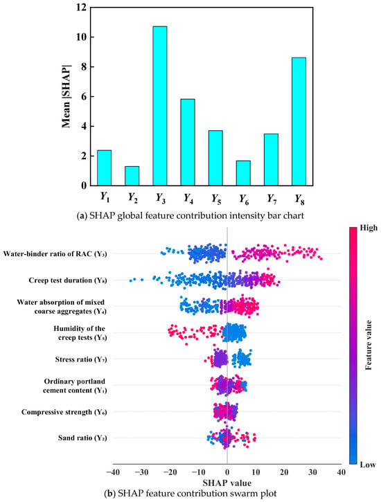
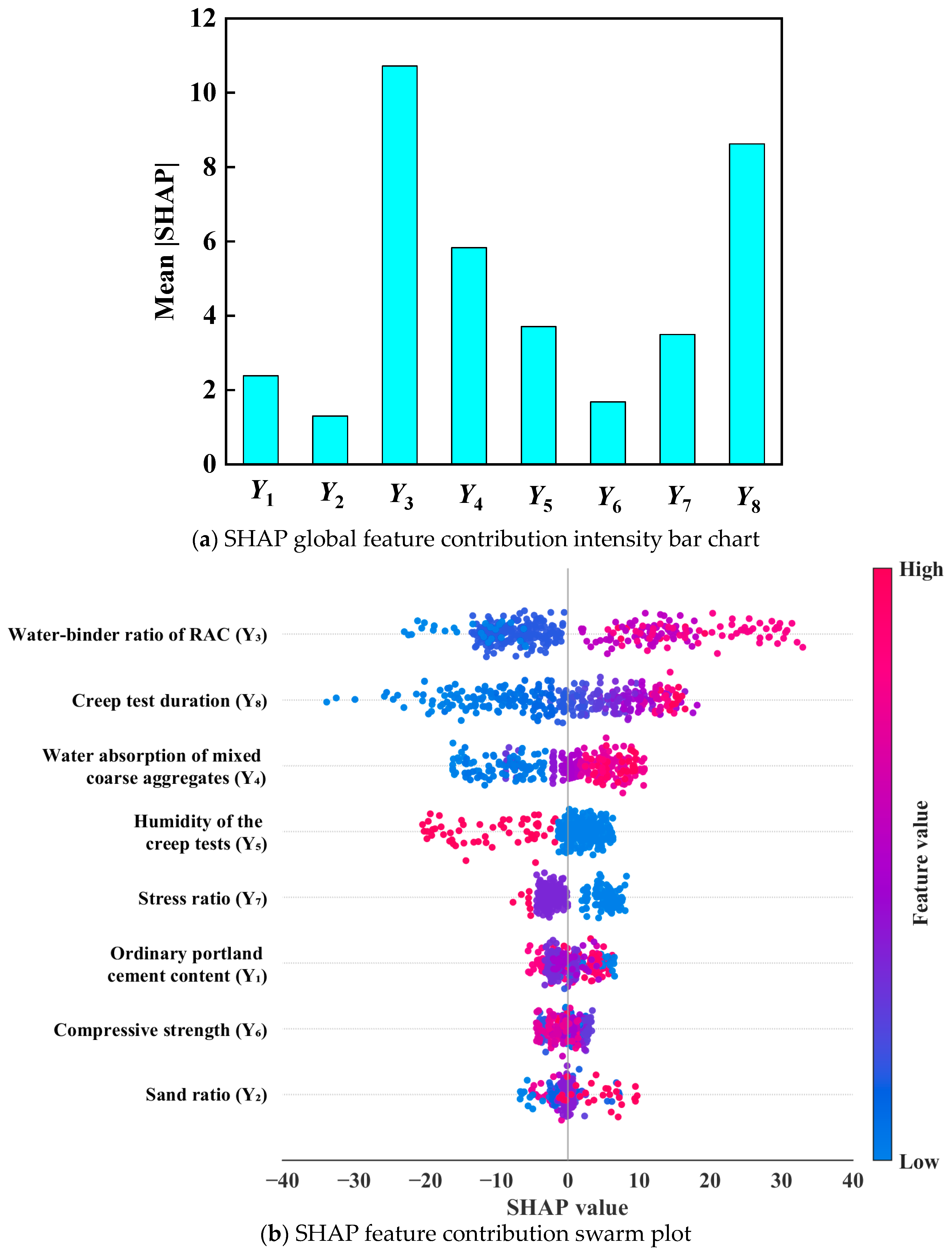
Figure 17 displays the SHAP analysis results derived from the optimal BPNN model. Figure 17a illustrates the global feature importance bar plot, where the mean absolute SHAP value (Mean |SHAP|) is adopted to evaluate the overall contribution of each input parameter to RAC creep prediction. Figure 17b presents the SHAP beeswarm plot, which is used to further show the distribution characteristics of SHAP values for different input parameters and their positive or negative contributions to the predicted creep values.

Figure 17. BPNN SHAP analysis results present the SHAP analysis results of the eight input parameters. The SHAP value distributions differ substantially across various input parameters, demonstrating that the BPNN model prediction of RAC creep is associated with multiple input parameters. Furthermore, the correlations between input parameters and predicted creep values are not purely linear but exhibit evident nonlinear characteristics and interval effects.

The results in Figure 17a show that the importance of the eight input parameters is ranked in descending order as follows: water-to-binder ratio (Y₃) > creep test time (Y₈) > water absorption of mixed coarse aggregates (Y₄) > humidity of the creep test (Y₅) > stress ratio (Y₇) > ordinary Portland cement content (Y₁) > compressive strength (Y₆) > sand ratio (Y₂). Among them, the Mean |SHAP| values of water-to-binder ratio (Y₃), creep test time (Y₈), and water absorption of mixed coarse aggregates (Y₄) are significantly higher than those of the other variables, indicating that these three parameters have relatively higher contributions to the RAC creep prediction results of the BPNN model. In particular, the water-to-binder ratio (Y₃) has the largest mean absolute SHAP value, indicating that it makes the most significant overall contribution to the model prediction results. In contrast, the Mean |SHAP| values of compressive strength (Y₆) and sand ratio (Y₂) are relatively low, indicating that their overall contributions in the current model are relatively weak.

Figure 17b further illustrates the distribution characteristics of the contribution values of each input parameter across different samples. Y₃ presents the widest SHAP value distribution range and thus shows the largest contribution variation to the BPNN model prediction of RAC creep. However, the considerable overlap of color-coded data points indicates that the positive and negative SHAP contributions of Y₃ show moderate consistency across different samples. The SHAP value distribution of Y₈ is slightly narrower than that of Y₃ still maintains a relatively large influence range on RAC creep prediction. Moreover, Y₈ exhibits continuous color variation and minor overlap between differently colored points, demonstrating a relatively clear and stable contribution direction to the model prediction results. Y₄ shows a regular color distribution pattern, with blue points mostly concentrated in the negative SHAP value region and red points predominantly distributed in the positive SHAP value region. This phenomenon indicates that higher values of Y₄ are generally associated with positive SHAP values and higher predicted creep values in the BPNN model. In contrast, Y₅ exhibits an obvious reverse influence pattern. The red points of Y₅ are mainly distributed in the negative SHAP value region, while blue points are concentrated near the zero line or within the positive SHAP value region, suggesting that higher values of Y5 are generally associated with negative SHAP values and lower predicted creep values in the model. Y₇ has a relatively narrow SHAP value distribution range. Although its data points show a certain degree of color differentiation, the overall influence magnitude on model prediction is limited. The SHAP values of Y₁, Y₆ and Y₂ are mostly concentrated near zero, indicating their relatively small contribution to the RAC creep prediction of the model. In addition, the substantial overlap of differently colored points suggests that the SHAP contributions of these three parameters are highly dispersed across different samples, and the positive or negative contributions of high and low feature values to the model prediction are not clearly distinguishable.

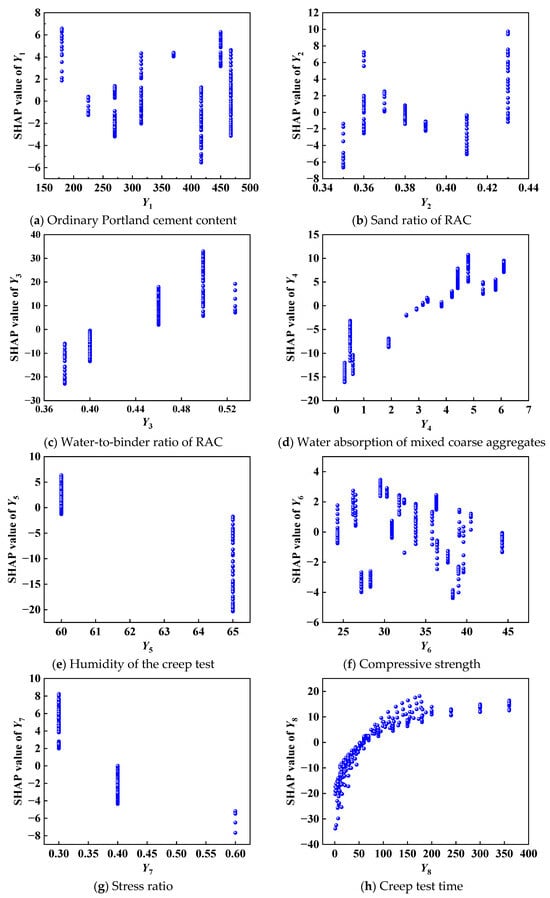
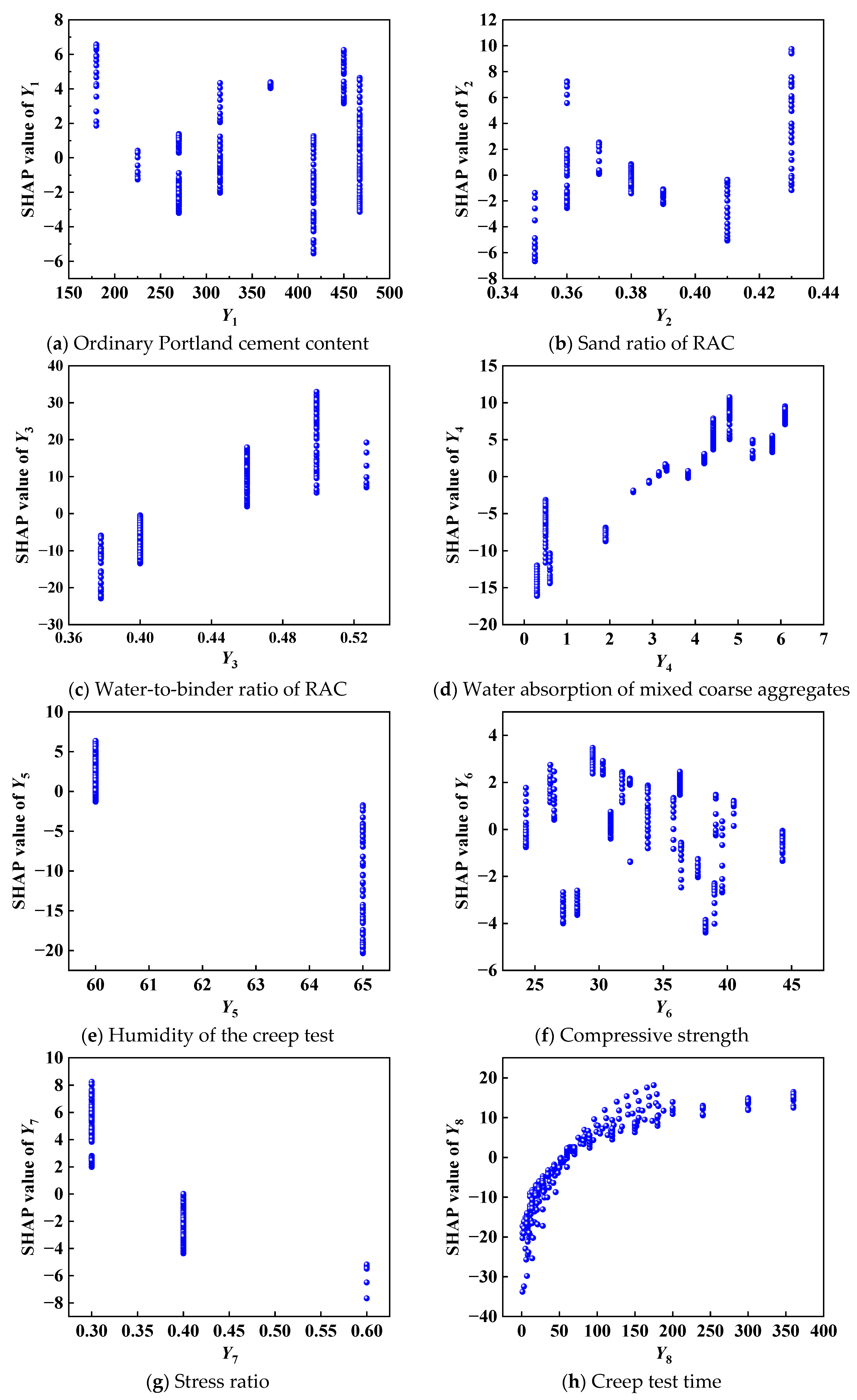
As shown in Figure 18a, ordinary Portland cement content (Y₁) presents distinct nonlinear fluctuation characteristics in its influence on RAC creep prediction. At relatively low Y₁ levels, SHAP values are predominantly positive, indicating that this parameter range increases the model-predicted creep values. As Y₁ increases, SHAP values fluctuate alternately between positive and negative regions, demonstrating that the contribution of Y₁ to the model prediction cannot be simply characterized as a single increasing or decreasing trend. This phenomenon suggests that the contribution of Y₁ to the model prediction varies under different combinations of input features, and no stable monotonic relationship can be identified.

Figure 18. SHAP analysis results of each input parameter.

As shown in Figure 18b, shows nonlinear and staged contribution patterns in the BPNN model prediction of RAC creep. At a relatively low level of Y₂, SHAP values are mainly distributed in the negative region, demonstrating that Y2 primarily provides a negative SHAP contribution to the predicted creep values within this interval. As the sand ratio increases, SHAP values fluctuate between positive and negative regions, presenting a non-monotonic variation pattern. When Y₂ reaches a relatively high level, the distribution range of SHAP values expands significantly, indicating that the model is more sensitive to this input parameter in the high sand ratio range.

As shown in Figure 18c, the water-to-binder ratio (Y₃) presents a distinct positive correlation with the predicted creep value. At low Y₃ levels, most SHAP values are negative, which is associated with lower predicted creep values of RAC in the model. As Y₃ increases, especially when Y₃ exceeds approximately 0.44, the SHAP values gradually turn positive and keep rising, demonstrating that a higher water-to-binder ratio is associated with elevated predicted creep values.

As shown in Figure 18d, the water absorption of mixed coarse aggregates (Y₄) exhibits an overall positive correlation trend according to its SHAP values. At a relatively low water absorption level, most SHAP values are negative, indicating that low water absorption values of mixed coarse aggregates are associated with lower predicted creep values. As water absorption increases, the SHAP values rise gradually and turn positive, and are associated with higher predicted creep values in the model.

As shown in Figure 18e, creep test humidity (Y₅) presents a distinct negative correlation with SHAP values. At a test humidity of 60%, most SHAP values are positive, implying that relatively low humidity conditions correspond to higher predicted creep values. When the humidity rises to 65%, the SHAP values turn distinctly negative, demonstrating that elevated humidity values are associated with lower model-predicted creep values.

As shown in Figure 18f, the SHAP values of compressive strength (Y₆) present a relatively narrow overall fluctuation range with no significant monotonic variation pattern. This indicates that, compared with key factors including the water-to-binder ratio, aggregate water absorption, and test humidity, compressive strength exerts a relatively weak direct contribution to the model-predicted creep values. As a macroscopic performance indicator determined by the combined effects of material composition, pore structure, curing age, and other factors, compressive strength may have a relatively complex relationship with model prediction due to its association with other input parameters, rather than showing an independent dominant contribution in the current model.

As shown in Figure 18g, the SHAP values of stress ratio (Y₇) present distinct zonal distribution characteristics. At a low stress ratio level, the corresponding SHAP values are predominantly positive. As the stress ratio rises to approximately 0.40 or higher, the SHAP values decline and eventually turn negative. Notably, from the perspective of the concrete creep mechanism, the stress ratio generally facilitates creep development. Accordingly, this finding cannot be simply interpreted as that a high stress ratio inhibits creep. Instead, it should be interpreted as a model-based association under the current dataset distribution. The observed SHAP pattern may be related to the combined distribution characteristics of the stress ratio and other input parameters, such as compressive strength and water-to-binder ratio. The model captures the comprehensive contribution of the stress ratio to RAC creep prediction under the joint characteristics of multiple input variables.

As shown in Figure 18h, the SHAP values of creep test time (Y₈) increase rapidly at the initial stage and then gradually stabilize. In the early loading period, SHAP values rise sharply from negative values, demonstrating that the positive contribution of test time to predicted creep values increases rapidly, indicating that test time has an increasing positive contribution to the model prediction during the early stage. With the continuous extension of test time, the growth rate of SHAP values gradually decreases and tends to be stable, indicating that the marginal contribution of test time to the model prediction gradually decreases at longer testing durations.

6. Comparison with Conventional RAC Creep Models

Zheng [41] established an RAC creep prediction model based on the ACI 209 model by introducing the influence coefficient of the RCA replacement ratio and the influence coefficient of the RCA pretreatment process, as shown in Equation (24).

$$\phi (t,t_0)=A{\gamma }_r{\gamma }_w(2.35{\gamma }_{1a}{\gamma }_{\mathit{RH}}{\gamma }_h{\gamma }_s{\gamma }_{\varphi }{\gamma }_a){\displaystyle \frac{{(t-t_0)}^{0.6}}{10+{(t-t_0)}^{0.6}}}$$

(24)

where t₀ is the curing age at loading, t is the age after loading, γ_1a is the adjustment coefficient for concrete loading age, γ_RH is the adjustment coefficient for environmental relative humidity, γ_h is the adjustment coefficient for specimen size, γ_s is the correction coefficient for concrete slump, γ_φ is the correction coefficient for fine aggregate content, γ_a is the correction coefficient for concrete air content, and A is the basic correction coefficient of the RAC model, with a value of 0.854, γ_r is the influence coefficient of RCA replacement ratio, and γ_w is the influence coefficient of RCA pretreatment process, which is taken as 1.0 when the RCA is untreated and 0.834 when the RCA is treated by the cement paste coating process.

Based on the ACI 209 model, Huang and Zheng [42] proposed a creep formula for recycled concrete, as shown in Equation (25).

$$\phi (t,t_0)=B{\gamma }_{r1}{\gamma }_{w1}(2.35{\gamma }_{1a}{\gamma }_{\mathit{RH}}{\gamma }_h{\gamma }_s{\gamma }_{\varphi }{\gamma }_a){\displaystyle \frac{{(t-t_0)}^{0.6}}{10+{(t-t_0)}^{0.6}}}$$

(25)

where B is the basic correction coefficient of the recycled aggregate concrete model, with a value of 0.7772, γ_r1 is the influence coefficient of recycled coarse aggregate replacement ratio, with a value of 1.198, γ_w1 is the correction coefficient of mineral admixtures.

Bai et al. [43] proposed a creep model for recycled concrete, as shown in Equations (26)–(32).

$$\phi (t,t_0)=2.35K_1{K}_2{K}_3{K}_4{K}_5{K}_6{\displaystyle \frac{{(t-t_0)}^{0.6}}{10+{(t-t_0)}^{0.6}}}$$

(26)

$$K_1=1.25\times {(t_0)}^{-0.118}$$

(27)

K₂ = 1.27 − 0.0067I_RH

(28)

K₃ = 1.1 − 0.000674(v/s)

(29)

K₄ = 0.82 + 0.00264S

(30)

K₅ = 0.88 + 0.0024f

(31)

K₆ = 0.46 + 0.09A_d

(32)

where t₀ is the curing age at loading, t is the age after loading, I_RH is the environmental relative humidity, v/s is the volume-to-surface ratio of the concrete member, S is the slump of concrete, f is the sand ratio, A_d is the air content of concrete.

It should be noted that Equations (24)–(32) yield the dimensionless creep coefficient φ(t, t₀), whereas the output variable Z of the machine learning models represents specific creep with a unit of 10⁻⁶ MPa⁻¹. To ensure dimensional consistency and comparability, the creep coefficients calculated by the conventional models were converted into specific creep before comparison. According to the definitions of creep coefficient and specific creep, the conversion can be expressed as Equation (33).

$$Z={\displaystyle \frac{\phi (t,t_0)}{E_c}}$$

(33)

where E_c is the elastic modulus of concrete at the loading age.

The additional parameters required by conventional creep models but not included in the machine learning database (e.g., replacement ratio, slump, air content, and v/s were determined according to the experimental conditions and parameter settings reported in the corresponding references). It should be noted that all conventional creep models were directly applied using their original formulations without recalibration against the present RAC database.

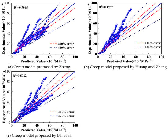
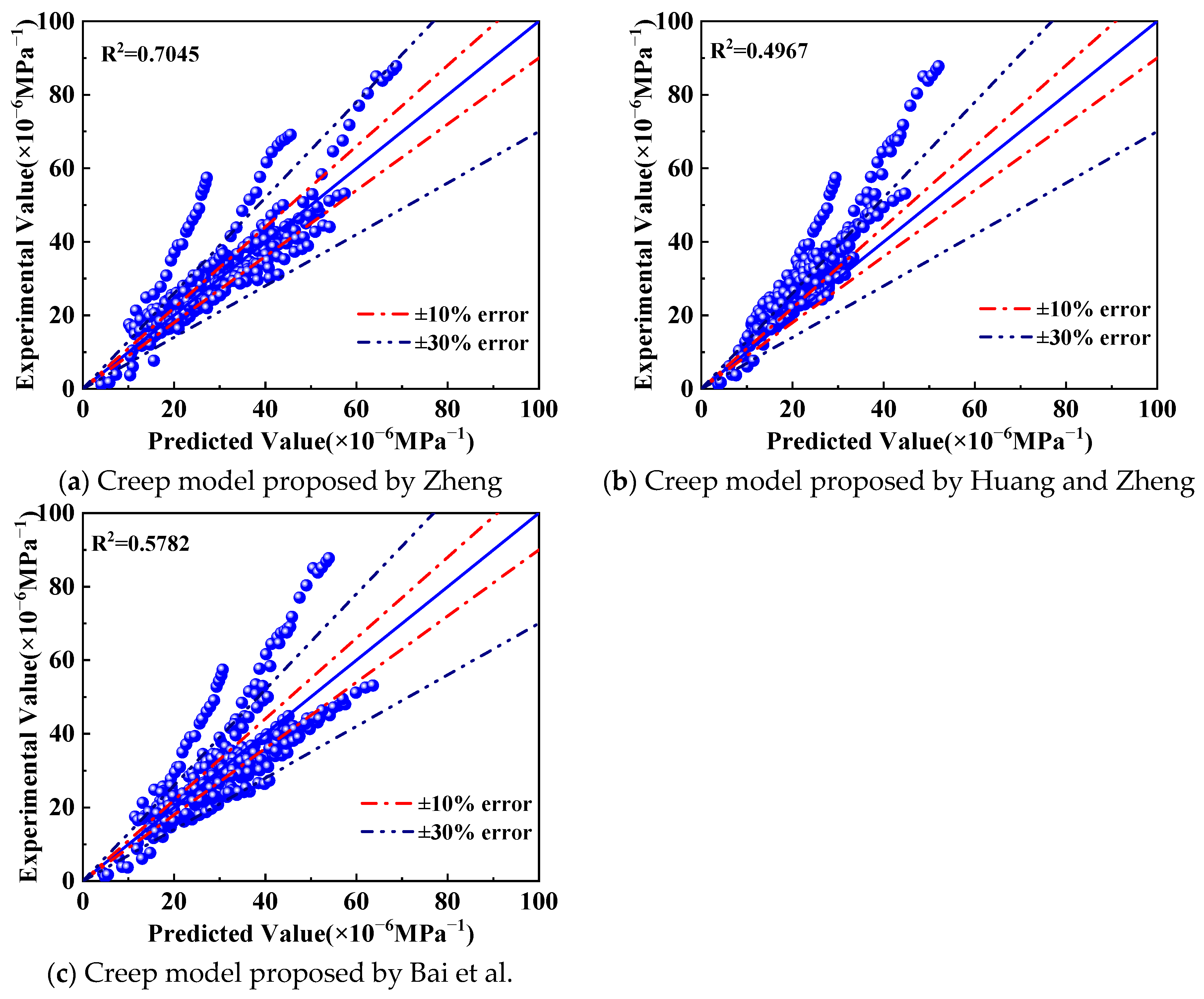
The input parameters of the training and test sets were substituted into the above formulas to obtain the predicted RAC creep values, which were then compared with the experimental results, as illustrated in Figure 19. The R² values of the creep calculation models proposed by Zheng [41], Huang and Zheng [42], and Bai et al. [43] are 0.7045, 0.4967, and 0.5782, respectively. A considerable number of predicted data points fall outside the ±30% error range, indicating that these conventional models exhibit relatively limited prediction accuracy when applied to the current RAC creep database. In comparison, the machine learning models developed in this study achieve higher prediction accuracy under the same experimental dataset. This improvement may be attributed to the ability of machine learning models to incorporate multiple input parameters and capture complex nonlinear relationships between variables. It should be noted that conventional creep models and machine learning models have different input structures because conventional models are generally established based on empirical formulations with limited parameters, whereas machine learning models can consider more comprehensive feature information. Therefore, the comparison in this study evaluates the prediction performance of different approaches under identical experimental conditions rather than identical input variables. The results demonstrate the potential of machine learning methods for RAC creep prediction.

Figure 19. Comparison between the predicted values of traditional models and the experimental values. (a) Creep model proposed by Zheng [41]; (b) creep model proposed by Huang and Zheng [42]; (c) creep model proposed by Bai et al. [43].

7. Conclusions and Prospects

Based on eight key influencing parameters, this study systematically investigates RAC creep behavior by developing five machine learning models and verifies the feasibility of machine learning methods for RAC creep prediction. The conclusions are summarized as follows:

(1) By comprehensively comparing four evaluation metrics of five machine learning models, namely BPNN, RBFNN, SVR, RF, and GEP, on both training and test sets, the BPNN model presents the optimal overall performance for RAC creep prediction, with the model performance ranked in descending order of RBFNN, SVR, RF, and GEP.

(2) Quantitative evaluation based on objective function reveals that the BPNN model obtains the minimum objective function value of 0.88, which corresponds to the highest prediction accuracy. The performance ranking of the remaining models is RBFNN, SVR, RF, and GEP. This result is consistent with the conclusions derived from the aforementioned model evaluation metrics, further verifying the superior predictive performance of the BPNN model in RAC creep prediction.

(3) The SHAP method was adopted to interpret the optimal BPNN model, revealing the dominant features contributing to RAC creep predictions. Water-to-binder ratio, creep test time, and water absorption of mixed coarse aggregates show the highest contributions to the model prediction, among which water-to-binder ratio contributes the most significantly. Creep test time presents a two-stage contribution pattern in the SHAP analysis, characterized by a rapid increase in SHAP values at the early stage and gradual stabilization at longer testing durations. Ambient humidity shows a negative SHAP contribution trend, whereas water absorption of coarse aggregates and water-to-binder ratio mainly show positive SHAP contribution trends. By comparison, cement content, sand ratio, and compressive strength show relatively limited contributions, with weak and dispersed SHAP contribution patterns.

(4) Comparative analysis with conventional RAC creep models demonstrates that the coefficient of determination values of traditional models range from 0.4967 to 0.7045, reflecting a much lower overall prediction accuracy compared with the machine learning models developed in this study. This indicates that conventional empirical models possess inherent limitations in characterizing the complex nonlinear creep behavior of RAC. In contrast, machine learning methods exhibit prominent advantages in prediction accuracy and engineering applicability.

Although this study investigated the effectiveness of machine learning methods in RAC creep prediction, certain limitations still exist. At present, only a few models can provide explicit analytical expressions, and only the water absorption characteristic of RCA was considered among the input parameters. Future research can introduce more RCA-related parameters and advanced machine learning algorithms to improve the generalization capability and engineering applicability of RAC creep prediction.

References

- Zhang, X.; Zhu, Y.; Fan, Y.; Zhou, G.; Huang, Y.; Li, M.; Shen, W. Experimental study on impact resistance and dynamic constitutive relation of steel fiber reinforced recycled aggregate concrete. Constr. Build. Mater. 2024, 449, 138396. [Google Scholar] [CrossRef] [Scilit]
- Hang, X.; Shen, Y.; Fan, Y.; Gao, X. Experimental study on the triaxial compression mechanical performance of basalt fiber-reinforced recycled aggregate concrete after exposure to high temperature. Case Stud. Constr. Mater. 2024, 20, e03026. [Google Scholar] [CrossRef] [Scilit]
- Zhang, X.; Zhu, Y.; Shen, Y.; Wang, J.; Fan, Y.; Gao, X.; Huang, Y. Compressive mechanical performance and microscopic mechanism of basalt fiber-reinforced recycled aggregate concrete after elevated temperature exposure. J. Build. Eng. 2024, 96, 110647. [Google Scholar] [CrossRef] [Scilit]
- Zhou, X.; Bai, L.; Rong, H.; Fan, X.; Zheng, J.; Geng, Y. An improved approach for the continuous retardation spectra of concrete creep and applications. Front. Mater. 2024, 11, 1340883. [Google Scholar] [CrossRef] [Scilit]
- Gong, F.; Yang, Y.; Li, P.; Wang, Z.; Zeng, B.; Jin, W.; Maekawa, K. Multi-physical analysis of saturation-dependent creep behavior for RC beam under sustained load and wet-dry cycles. Eng. Struct. 2024, 309, 117976. [Google Scholar] [CrossRef] [Scilit]
- Geng, Y.; Wang, Y.; Chen, J. Creep behaviour of concrete using recycled coarse aggregates obtained from source concrete with different strengths. Constr. Build. Mater. 2016, 128, 199–213. [Google Scholar] [CrossRef] [Scilit]
- Seara-Paz, S.; González-Fonteboa, B.; Martínez-Abella, F.; González-Taboada, I. Time-dependent behaviour of structural concrete made with recycled coarse aggregates. Creep and shrinkage. Constr. Build. Mater. 2016, 122, 95–109. [Google Scholar] [CrossRef] [Scilit]
- Chen, J.; Zhou, Y.; Yin, F. A practical equation for the elastic modulus of recycled aggregate concrete. Buildings 2022, 12, 187. [Google Scholar] [CrossRef] [Scilit]
- Alibeigibeni, A.; Stochino, F.; Zucca, M.; López Gayarre, F. Enhancing concrete sustainability: A critical review of the performance of recycled concrete aggregates (RCAs) in structural concrete. Buildings 2025, 15, 1361. [Google Scholar] [CrossRef] [Scilit]
- Hansen, T.C. Recycled aggregates and recycled aggregate concrete second state-of-the-art report developments 1945–1985. Mater. Struct. 1986, 19, 201–246. [Google Scholar] [CrossRef] [Scilit]
- Wang, Q.; Liu, F.; Liu, Y.; Zhang, X.; Li, J.; Wang, H. Creep performance and prediction of recycled coarse aggregate concrete considering the influence of humidity boundary conditions. Arch. Civ. Mech. Eng. 2025, 25, 301. [Google Scholar] [CrossRef] [Scilit]
- Domingo, A.; Lázaro, C.; Gayarre, F.L.; Serrano, M.A.; López-Colina, C. Long term deformations by creep and shrinkage in recycled aggregate concrete. Mater. Struct. 2010, 43, 1147–1160. [Google Scholar] [CrossRef] [Scilit]
- Lye, C.Q.; Dhir, R.K.; Ghataora, G.S. Creep strain of recycled aggregate concrete. Constr. Build. Mater. 2016, 102, 244–259. [Google Scholar] [CrossRef] [Scilit]
- Tam, V.W.Y.; Kotrayothar, D.; Xiao, J. Long-term deformation behaviour of recycled aggregate concrete. Constr. Build. Mater. 2015, 100, 262–272. [Google Scholar] [CrossRef] [Scilit]
- Zhao, M.Z.; Zhang, H.; Geng, Y.; Wang, Y.; Chen, J. Basic creep behavior and modeling of recycled coarse and fine aggregate concrete. Constr. Build. Mater. 2023, 389, 131724. [Google Scholar] [CrossRef] [Scilit]
- Domingo-Cabo, A.; Lázaro, C.; López-Gayarre, F.; Serrano-López, M.A.; López-Colina, C.; Serna, P. Creep and shrinkage of recycled aggregate concrete. Constr. Build. Mater. 2009, 23, 2545–2553. [Google Scholar] [CrossRef] [Scilit]
- Liu, Y.; Li, Y.; Mu, J.; Zhang, W.; Wang, X. Modeling and analysis of creep in concrete containing supplementary cementitious materials based on machine learning. Constr. Build. Mater. 2023, 392, 131911. [Google Scholar] [CrossRef] [Scilit]
- Hong, S.H.; Choi, J.S.; Yuan, T.F.; Yoon, Y.S. A review on concrete creep characteristics and its evaluation on high-strength lightweight concrete. J. Mater. Res. Technol. 2023, 22, 230–251. [Google Scholar] [CrossRef] [Scilit]
- Neville, A.M.; Meyers, B.L. Creep of concrete: Influencing factors and prediction. Spec. Publ. 1964, 9, 1–33. [Google Scholar]
- Li, K.; Jing, H.; Wang, J. Combining machine learning methods with feature selection for predicting concrete basic creep. J. Asian Archit. Build. Eng. 2025. [Google Scholar] [CrossRef] [Scilit]
- Bažant, Z.P.; Jirásek, M.; Hubler, M.H.; Wendner, R.; Leps, M.; Šmilauer, V.; Vráblík, L.; Carol, I.; Cedolin, L.; Cusatis, G.; et al. RILEM draft recommendation: TC-242-MDC multi-decade creep and shrinkage of concrete: Material model and structural analysis. Model B4 for creep, drying shrinkage and autogenous shrinkage of normal and high-strength concretes with multi-decade applicability. Mater. Struct. 2015, 48, 753–770. [Google Scholar]
- Yang, Y.; Zhou, C.; Peng, J.; Zhang, Y.; Li, J. Hybrid model-driven and data-driven method for predicting concrete creep considering uncertainty quantification. Front. Struct. Civ. Eng. 2024, 18, 1524–1539. [Google Scholar] [CrossRef] [Scilit]
- Fan, Z.; Zhan, Y.; Xiang, T.; Li, W.; Zhang, H. A time-series deep learning model for predicting concrete shrinkage and creep verified with in-situ and laboratory test data. Constr. Build. Mater. 2024, 447, 138140. [Google Scholar] [CrossRef] [Scilit]
- Munir, M.J.; Kazmi, S.M.S.; Wu, Y.F.; Lin, X.; Li, J. Development of novel design strength model for sustainable concrete columns: A new machine learning-based approach. J. Clean. Prod. 2022, 357, 131988. [Google Scholar] [CrossRef] [Scilit]
- Tran, V.Q.; Dang, V.Q.; Ho, L.S. Evaluating compressive strength of concrete made with recycled concrete aggregates using machine learning approach. Constr. Build. Mater. 2022, 323, 126578. [Google Scholar] [CrossRef] [Scilit]
- Haque, M.A.; Chen, B.; Javed, M.F.; Jalal Fazal, E. Evaluating the mechanical strength prediction performances of fly ash-based MPC mortar with artificial intelligence approaches. J. Clean. Prod. 2022, 355, 131815. [Google Scholar] [CrossRef] [Scilit]
- Feng, D.C.; Liu, Z.T.; Wang, X.D.; Chen, Y.; Chang, J.Q.; Wei, D.F.; Jiang, Z.W. Machine learning-based compressive strength prediction for concrete: An adaptive boosting approach. Constr. Build. Mater. 2020, 230, 117000. [Google Scholar] [CrossRef] [Scilit]
- Li, L.; Su, L.; Guo, B.; Zhang, Y.; Wang, H. Prediction and prevention of concrete chloride penetration: Machine learning and MICP techniques. Front. Mater. 2024, 11, 1445547. [Google Scholar] [CrossRef] [Scilit]
- Taffese, W.Z.; Hilloulin, B.; Villagran Zaccardi, Y.; Marani, A.; Nehdi, M.L.; Hanif, M.U.; Kamath, M.; Nunes, S.; von Greve-Dierfeld, S.; Kanellopoulos, A. Machine learning in concrete durability: Challenges and pathways identified by RILEM TC 315-DCS towards enhanced predictive models. Mater. Struct. 2025, 58, 145. [Google Scholar] [CrossRef] [Scilit]
- Ni, B.; Rahman, M.Z.; Guo, S.; Wang, H.; Li, Z. A review on properties and multi-objective performance predictions of concrete based on machine learning models. Mater. Today Commun. 2025, 44, 112017. [Google Scholar] [CrossRef] [Scilit]
- Li, W.; Li, H.; Liu, C.; Zhang, Y.; Wang, J. Concrete creep prediction based on improved machine learning and game theory: Modeling and analysis methods. Buildings 2024, 14, 3627. [Google Scholar] [CrossRef] [Scilit]
- Liang, M.; Chang, Z.; Wan, Z.; Wang, Y.; Li, H. Interpretable Ensemble-Machine-Learning models for predicting creep behavior of concrete. Cem. Concr. Compos. 2022, 125, 104295. [Google Scholar] [CrossRef] [Scilit]
- Li, K.; Long, Y.; Wang, H.; Zhang, J.; Liu, Y. Modeling and sensitivity analysis of concrete creep with machine learning methods. J. Mater. Civ. Eng. 2021, 33, 04021206. [Google Scholar] [CrossRef] [Scilit]
- Bouras, Y.; Li, L. Prediction of high-temperature creep in concrete using supervised machine learning algorithms. Constr. Build. Mater. 2023, 400, 132828. [Google Scholar] [CrossRef] [Scilit]
- Gao, C.; Luo, C.; Zhang, B.; Li, X.; Wang, J. Creep behavior evaluation of recycled aggregate concrete using machine learning technology. J. Build. Eng. 2025, 99, 111538. [Google Scholar] [CrossRef] [Scilit]
- Feng, J.; Zhang, H.; Gao, K.; Liu, Y.; Wang, Y. Efficient creep prediction of recycled aggregate concrete via machine learning algorithms. Constr. Build. Mater. 2022, 360, 129497. [Google Scholar] [CrossRef] [Scilit]
- Rong, X.; Liu, Y.; Chen, P.; Wang, H.; Zhang, J. Prediction of creep of recycled aggregate concrete using back-propagation neural network and support vector machine. Struct. Concr. 2023, 24, 2229–2244. [Google Scholar] [CrossRef] [Scilit]
- Fan, Y.H.; Niu, H.C.; Zhang, X.G. Creep test of recycled aggregate concrete and influence mechanism of old attached mortar. J. Build. Mater. 2020, 23, 596–602. (In Chinese) [Google Scholar]
- Fan, Y.H.; Xiao, J.Z.; Tam, V.W.Y. Effect of old attached mortar on the creep of recycled aggregate concrete. Struct. Concr. 2014, 15, 169–178. [Google Scholar] [CrossRef] [Scilit]
- Huang, H.S.; Zheng, J.L. Prediction adequacy of creep of recycled concrete influenced by the water absorption in recycled aggregates. J. Test. Eval. 2019, 47, 2926–2946. [Google Scholar] [CrossRef] [Scilit]
- Zheng, X. Experimental Research on Creep Performance of Recycled Aggregate Concrete with Recycled Coarse Aggregate Pretreatment. Master’s Thesis, Fuzhou University, Fuzhou, China, 2013. (In Chinese) [Google Scholar]
- Huang, H.S.; Zheng, J.L. Effects of fly ash and slag powder on creep properties of recycled aggregate concrete. J. Fuzhou Univ. (Nat. Sci. Ed.) 2017, 45, 206–211. (In Chinese) [Google Scholar]
- Bai, G.L.; Qi, H.; Liu, C. Creep test and prediction model of recycled aggregate concrete. J. Build. Struct. 2016, 37, 121–126. (In Chinese) [Google Scholar]
- Li, Y.; Li, H.; Shen, J. The study of effect of carbon nanotubes on the compressive strength of cement-based materials based on machine learning. Constr. Build. Mater. 2022, 358, 129435. [Google Scholar] [CrossRef] [Scilit]
- Ali, P.J.M.; Faraj, R.H.; Koya, E. Data normalization and standardization: A technical report. Mach. Learn. Tech. Rep. 2014, 1, 1–6. [Google Scholar]
- Smith, J.S.; Wu, B.; Wilamowski, B.M. Neural network training with Levenberg–Marquardt and adaptable weight compression. IEEE Trans. Neural Netw. Learn. Syst. 2018, 30, 580–587. [Google Scholar] [CrossRef] [Scilit] [PubMed]
- Feng, J.; Zhang, H.; Gao, K.; Liu, Y.; Wang, Y. A machine learning and game theory-based approach for predicting creep behavior of recycled aggregate concrete. Case Stud. Constr. Mater. 2022, 17, e01653. [Google Scholar] [CrossRef] [Scilit]
Disclaimer/Publisher’s Note: The statements, opinions and data contained in all publications are solely those of the individual author(s) and contributor(s) and not of MDPI and/or the editor(s). MDPI and/or the editor(s) disclaim responsibility for any injury to people or property resulting from any ideas, methods, instructions or products referred to in the content. |
© 2026 by the authors. Licensee MDPI, Basel, Switzerland. This article is an open access article distributed under the terms and conditions of the Creative Commons Attribution (CC BY) license.