


Abstract
Emotion recognition from electroencephalography (EEG) signals is a central problem in affective computing. This study benchmarks seven classical machine learning models—XGBoost, LightGBM, Random Forest, Support Vector Machine (SVM), K-Nearest Neighbors (KNN), Decision Tree, and Logistic Regression—for multiclass EEG emotion classification on the FACED dataset, which provides fine-grained labels across nine emotion categories (amusement, inspiration, joy, tenderness, anger, fear, disgust, sadness, and neutral) from 123 participants. We extract Differential Entropy (DE) features across five frequency bands and, using an identical feature-and-preprocessing pipeline, evaluate all models under three distinct protocols that differ only in how the data are partitioned: (i) an intra-subject protocol, in which a separate model is trained and tested within each participant and the per-participant scores are averaged; (ii) a pooled segment-level protocol, in which segments from all participants are mixed so that segments from the same participant may fall in both training and test sets; and (iii) a strict subject-independent protocol, in which all segments from any given participant are kept together on one side of the training and test split, so that test participants are never seen during training. Under the intra-subject protocol, the best model (LightGBM) reaches 85.4% accuracy; under the pooled segment-level protocol the best model reaches 56.4%; and under the subject-independent protocol the best model (SVM with an RBF kernel) achieves only 18.2% accuracy—above the 11.1% chance level but far below the other two settings. We provide reproducible baselines under all three protocols and argue that subject-independent evaluation is essential for meaningful benchmarking on FACED.
1. Introduction
Emotion recognition from electroencephalography (EEG) activity has become one of the most significant problems in affective computing, motivated by the goal of bridging the gap between humans and computers through the interpretation of emotional states from brain signals. EEG-based emotion classification offers a physiologically grounded and temporally rich characterization of a user’s affective state. In recent years, interest has grown in developing machine learning models that decode emotion-related information from EEG signals using publicly available datasets such as DEAP (Database for Emotion Analysis using Physiological Signals), SEED (SJTU Emotion EEG Dataset), and DREAMER. Among these, the Finer-grained Affective Computing EEG Dataset (FACED) occupies a distinctive position, as it provides fine-grained labels across nine emotion categories from a large participant pool.
Classical machine learning models have long served as the first step in the EEG emotion classification pipeline. Models such as Support Vector Machines (SVM), K-Nearest Neighbors (KNN), Random Forests (RF), and gradient-boosting methods are interpretable and often perform competitively when data are limited [1]. Such approaches provide clear performance benchmarks and enable comparisons across datasets and feature representations.
Ensemble methods such as Random Forest and Extreme Gradient Boosting (XGBoost) are popular because they resist overfitting and scale to high-dimensional data. Yuvaraj et al. [1] evaluated ensemble models using spatio-temporal features on SEED and SEED-IV and reported strong cross-subject performance. KNN and SVM are similarly widely used, as they are simple to implement and perform well on small and medium datasets [2].
Several studies have compared these models across different feature-extraction methods, including Differential Entropy (DE), Power Spectral Density (PSD), and band-power features. For example, Murungi et al. [3] emphasized the pedagogical value of classical models in supporting reproducibility and accessibility in EEG research.
A well-known gap exists between the theoretical potential of baseline models and their practical performance, particularly with respect to inter-subject variability, noise sensitivity, and generalization in the multiclass case. Critically, the choice of evaluation protocol has a large effect on reported performance: when segments from the same participant appear in both training and test sets, models can exploit participant-specific information, so the resulting accuracy does not reflect generalization to unseen participants. Such intra-subject evaluation is nevertheless a valid protocol for personalized systems; it simply answers a different question from subject-independent evaluation. This distinction between within-subject, pooled, and subject-independent evaluation is central to the present work.
This paper provides a systematic benchmark of classical baseline models for multiclass emotion classification on the FACED dataset under three protocols—intra-subject, pooled segment-level, and subject-independent—using an identical feature-and-preprocessing pipeline so that the only difference between the settings is how the data are partitioned. By quantifying the resulting progression, we establish reproducible baselines and highlight the importance of choosing the evaluation protocol that matches the intended use of a model.
2. Literature Review
2.1. Overview of the FACED Dataset
This study uses the FACED (Finer-grained Affective Computing EEG Dataset) [4], which comprises recordings from 123 participants across 32 EEG channels, labeled according to the nine discrete emotion categories used in the dataset: amusement, inspiration, joy, tenderness, anger, fear, disgust, sadness, and neutral. Its large sample size and balanced category design make it well suited for multiclass classification, distinguishing it from earlier benchmarks such as DEAP [5] and SEED [6], which are limited to binary or three-class emotion paradigms.
Recent deep learning methods report strong results on FACED, though under differing evaluation protocols that must be distinguished carefully. Under a cross-subject (subject-independent) protocol, in which no test participant is seen during training, the dataset authors report CLISA (Contrastive Learning for Inter-Subject Alignment) at 42.4 ± 1.2% using a ten-fold subject-wise procedure [4], and a traditional DE+SVM baseline at 35.2 ± 1.0% [4]; DAEST (Dynamic-Attention-based EEG State Transition modeling) reports 59.3 ± 7.7% under a cross-subject protocol [7]. By contrast, methods evaluated under an intra-subject protocol, in which each model is trained and tested within the same participant, report substantially higher figures—for example, the Lipschitz Continuity-Constrained Emotion Recognition Ensemble Learning (LEREL) framework reports 83.0% on FACED as an explicitly intra-subject method [8]. These two families of results are not directly comparable, and conflating them is precisely the kind of protocol confusion this study seeks to make explicit. The cross-subject figures illustrate both the difficulty of cross-subject nine-class recognition and the benefit of methods designed specifically for inter-subject alignment.
2.2. Classical Machine Learning Models Overview
Classical machine learning models are well-established baselines in affective computing. The Extreme Gradient Boosting (XGBoost) algorithm is a generalization of gradient-boosted decision trees that trains an ensemble of decision trees efficiently on large, high-dimensional datasets and incorporates regularization to improve performance [9]. The Light Gradient Boosting Machine (LightGBM) is a boosting algorithm optimized for speed and memory efficiency, using histogram-based decision-tree learning and leaf-wise growth [10]. Both methods have been widely applied to biomedical signal classification owing to their robustness and their ability to capture non-linear relationships [11].
Decision Trees are simple, interpretable rule-based classifiers; despite their tendency to overfit, they support feature-relevance analysis and form the building block of ensemble methods [12]. Random Forest aggregates many decision trees to improve generalization and reduce overfitting [13], and is effective on noisy EEG data [1]. SVMs find optimal separating hyperplanes in a high-dimensional feature space, often using non-linear kernels such as the radial basis function (RBF) kernel [14], and are well suited to high-dimensional DE features [4]. KNN is a non-parametric method that classifies points by the majority class of their nearest neighbors [15], and is effective when local structure in the feature space is informative [16].
2.3. Classical Machine Learning Models in EEG Emotion Classification
Classical models such as SVM, KNN, Linear Discriminant Analysis (LDA), Logistic Regression, Decision Trees, and Random Forest are widely used for EEG-based emotion classification [16]. These models rely on hand-crafted features such as DE, PSD, or time-frequency representations, and are valued for their interpretability and efficiency [17]. On the FACED dataset, DE+SVM achieves 78.8 ± 1.0% intra-subject accuracy for binary classification and 51.1 ± 0.9% for the nine-class task under the original authors’ protocol [4].
Beyond FACED, classical models have been applied to DEAP and SEED. A study on DEAP compared multiple classical models with and without principal component analysis (PCA) [18]; SVM with PCA achieved an F1-score of 84.73% for binary arousal classification, while Logistic Regression and Decision Trees plateaued between 55% and 68% accuracy. On the SEED three-class task, SVM has been reported to reach 91.07% accuracy [6]. These results confirm the competitiveness of classical models on coarse-grained tasks, but also foreshadow the sharp performance drop that occurs as class granularity increases and as evaluation moves from intra-subject to subject-independent protocols.
2.4. Research Gaps and Contributions
Despite its richness, the FACED dataset has been underutilized for systematic classical benchmarking, and existing classical evaluations rarely make the distinction between within-subject, pooled, and subject-independent protocols explicit. Many benchmarks use pooled segment-level cross-validation that mixes segments from the same participant across training and test folds, which overestimates generalization to unseen participants. To address these gaps, this work presents (i) a systematic evaluation of seven classical models using DE features under three protocols—intra-subject, pooled segment-level, and strict subject-independent, and (ii) a direct quantification of the performance progression across the three protocols. We provide a reproducible pipeline and results under all three protocols.
3. Materials and Methods
3.1. Dataset
We use the FACED dataset [4], which contains EEG recordings from 123 participants who each viewed 28 video clips designed to elicit nine emotion categories. Recordings were made with 32 electrodes, and DE features were computed in five conventional frequency bands: delta (: 1–4 Hz), theta (: 4–8 Hz), alpha (: 8–14 Hz), beta (: 14–30 Hz), and gamma (: 30–47 Hz). A full description of the dataset is given in Section 2.1. Each participant viewed three clips for each of the eight emotion categories and four neutral clips, and each clip is represented by 30 one-second segments (epochs), giving 840 segments per participant and 103,320 segments in total. The number of segments per class is therefore 11,070 for each of the eight emotion categories and 14,760 for the neutral category.
3.2. Preprocessing and Feature Extraction with Differential Entropy (DE)
This work used the precomputed Differential Entropy (DE) features released with the FACED dataset [4], for which all preprocessing and feature extraction were performed by the dataset authors. According to the dataset description, the raw EEG was band-pass filtered (0.05–47 Hz), channels with excessive outlier proportions were interpolated, ocular artifacts were removed by independent component analysis (ICA), and the signal was re-referenced to the common average; the cleaned recordings were then divided into non-overlapping one-second segments, filtered into the five frequency bands, and DE was computed for each band and channel. For a band-filtered signal following a Gaussian distribution, DE has the closed form
where is the vector of the N samples of the band-filtered EEG signal of one channel within a one-second segment, and is its variance. Computing DE for each of the 32 channels in each of the five frequency bands yields a 160-dimensional feature vector (32 channels × 5 bands) per one-second segment. This vector is the feature representation used by all classical models.
Feature standardization is applied by z-scoring each feature, and in every protocol the standardization statistics (mean and standard deviation) are fitted on the training partition only and then applied unchanged to the held-out data, so that no information from the test partition influences training. The exact training partition on which the scaler is fitted therefore depends on the protocol: within each participant for the intra-subject protocol, on the pooled training set for the segment-level protocol, and on the training participants for the subject-independent protocol.
3.3. Models and Evaluation Protocols
Seven classical models were evaluated: XGBoost, LightGBM, Random Forest, SVM, KNN, Decision Tree, and Logistic Regression, implemented in scikit-learn (v1.7.0), XGBoost (v3.2.0), and LightGBM (v4.6.0), using Python 3.10.9 and NumPy 1.26.4. Hyperparameters are summarized in Table 1.
Table 1.
Fixed hyperparameter values used for the classical machine learning models. The same values are used across all three protocols; no hyperparameter search was performed for the main experiments (see Appendix A for a sensitivity analysis).
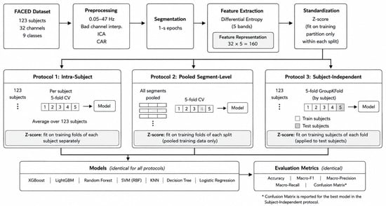
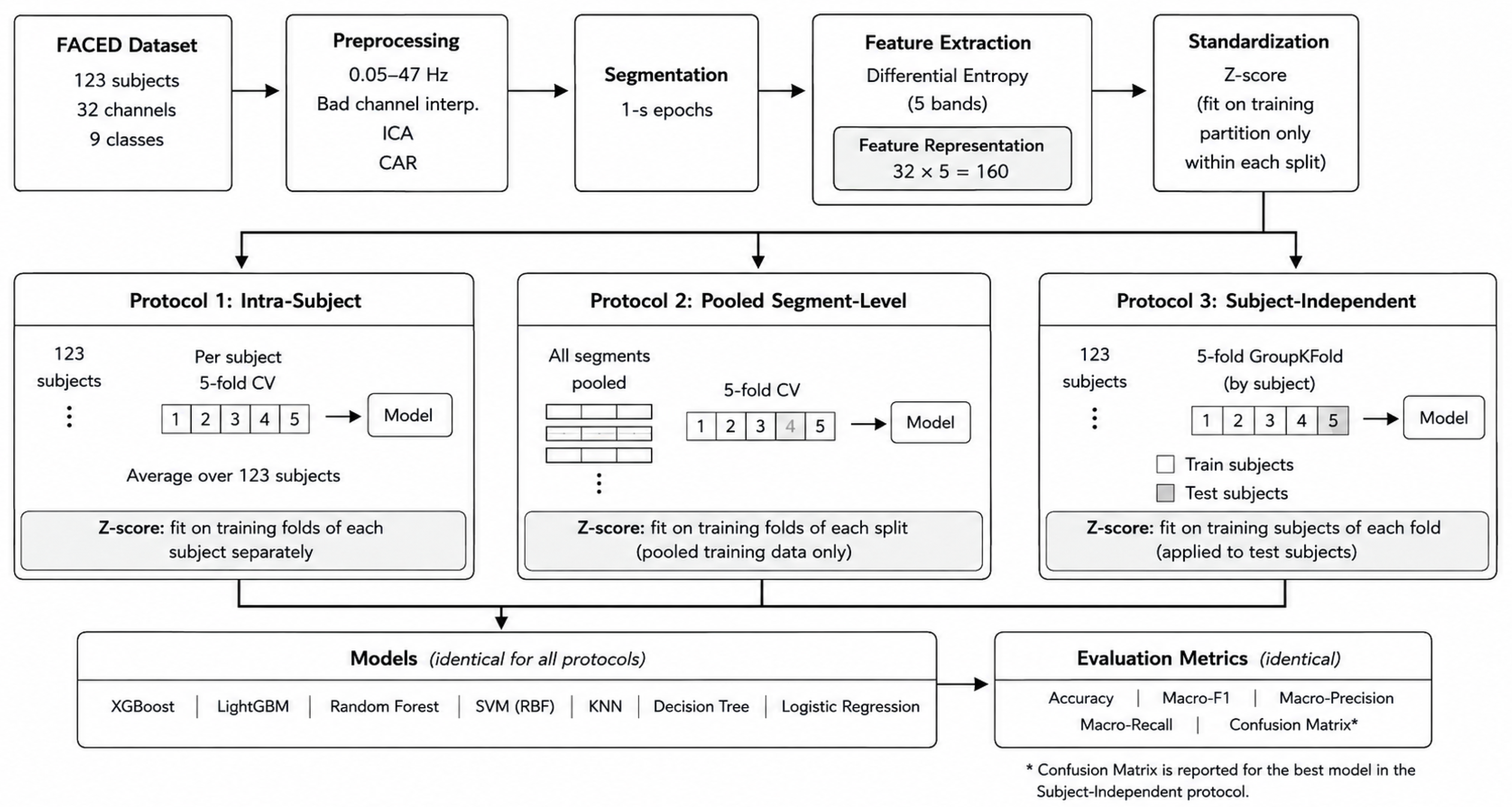
We evaluate all models under three protocols that share an identical feature-and-preprocessing pipeline and differ only in how the data are partitioned. Feature standardization is fitted on the training partition only in every case, so that no test statistics leak into training. Figure 1 summarizes the full pipeline and the three protocols.
Figure 1.
Overview of the experimental pipeline: feature extraction and standardization, the three evaluation protocols, the seven classifiers, and the evaluation metrics.
The intra-subject protocol trains and evaluates a separate model within each participant. For each of the 123 participants, that participant’s segments are split using 5-fold stratified cross-validation, a model is trained and tested entirely on data from that single participant, and the resulting per-participant accuracy is averaged across the five folds. The reported figure is then the mean (and standard deviation) of these per-participant scores across all participants. This is the conventional meaning of intra-subject evaluation: classification is performed individually for each person and then summarized across people.
The pooled segment-level protocol mixes the one-second segments of all participants and splits them into training (80%) and test (20%) sets, stratified by class and without any grouping by participant, so that segments from the same participant may fall in both sets. This is the protocol most commonly used, often implicitly, in prior classical benchmarks; it does not correspond to either within-subject or cross-subject deployment.
The subject-independent protocol splits the participants, rather than the segments, into a training set of 98 participants and a test set of 25 participants, so that all segments from a given participant fall on the same side of the split and no participant appears in both sets. This is the only one of the three protocols that measures generalization to unseen subjects. The stability of this single-split estimate is examined with 5-fold group-wise cross-validation in Appendix A.
To keep the seven-model, three-protocol comparison computationally tractable and to hold the modelling budget identical across all models, every model uses a single fixed set of hyperparameters (Table 1), held constant across all three protocols. These values correspond to library defaults or commonly used settings for each model family; for example, the SVM uses with set by the scale heuristic. To assess whether this choice affects the results or the model ranking, we performed a hyperparameter sensitivity analysis for SVM and LightGBM under the subject-independent protocol (Appendix A). The default SVM configuration achieved the highest accuracy among the nine SVM configurations evaluated, and no LightGBM configuration exceeded it, so the relative ranking of the two models is unchanged by tuning. All models and data splits use a fixed random seed of 42. We report accuracy and macro F1-score.
4. Results
4.1. Intra-Subject Performance
Table 2 reports performance under the intra-subject protocol, in which a separate model is trained and evaluated within each participant and the per-participant accuracies are averaged across participants. In this setting, LightGBM is the best model at 85.4% accuracy, with XGBoost (84.4%) and Random Forest (83.0%) close behind.
Table 2.
Intra-subject performance of classical models on the FACED nine-class task (a separate model for each participant; mean ± standard deviation across the 123 participants).
4.2. Pooled Segment-Level Performance
Table 3 reports performance under the pooled segment-level protocol, in which segments from all participants are mixed and split without grouping, so that segments from the same participant may fall in both the training and test sets. In this setting, Random Forest is the best model at 56.4% accuracy, with LightGBM (55.8%) and XGBoost (53.3%) close behind. These figures lie between the intra-subject and subject-independent results.
Table 3.
Pooled segment-level performance of classical models on the FACED nine-class task (stratified 80/20 split of all segments without participant grouping, random seed 42).
4.3. Subject-Independent Nine-Class Classification Performance
Table 4 reports performance under the subject-independent protocol, using the same features and preprocessing as the other two settings, with standardization fitted on the training participants only. Performance drops sharply. SVM with an RBF kernel is now the best model at 18.2% accuracy and 16.8% macro F1-score, followed closely by Logistic Regression, Random Forest, and XGBoost. All models exceed the 11.1% chance level, although Decision Tree and KNN do so only marginally, indicating that emotion-relevant information is present but only weakly recoverable across participants with classical models and DE features.
Table 4.
Subject-independent performance of classical models on the FACED nine-class task (held-out split at the participant level: 98 training and 25 test participants, random seed 42).
Several factors explain the sharp drop in performance under the subject-independent protocol. First, DE features vary substantially between individuals owing to differences in anatomy, electrode contact and impedance, and baseline spectral power, so the feature distribution of an unseen participant differs from those seen during training, and the classical models evaluated here have no mechanism for aligning feature distributions across participants. Second, individuals differ in how strongly and in what way the same stimulus elicits an emotional response, so the mapping from EEG features to emotion labels is itself participant-dependent. Third, in the intra-subject and pooled protocols, segments were assigned to folds at the segment level, so segments from the same participant, and from the same video trial, could appear in both the training and test sets; flexible models such as tree ensembles can exploit such shared participant- and trial-specific structure, which is unavailable in the subject-independent protocol. This also explains why the ensembles lose their advantage over SVM and Logistic Regression once test participants are held out.
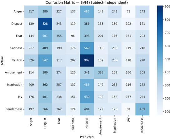
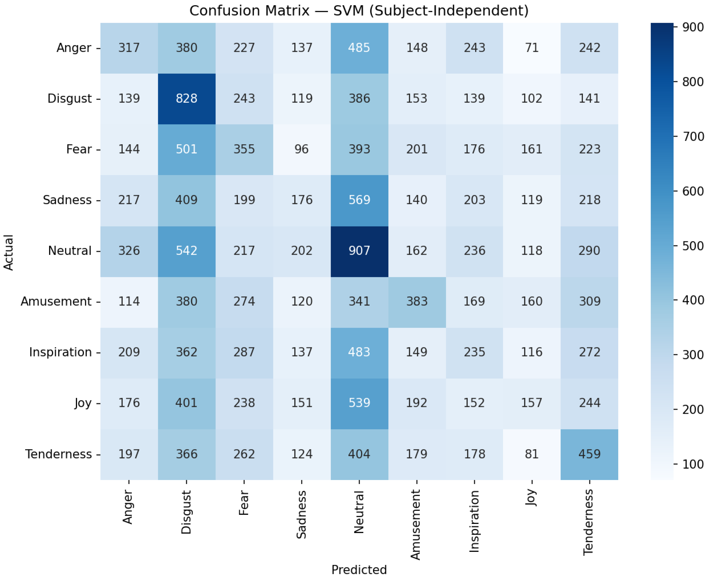
Per-class results for the best subject-independent model (SVM) are shown in Table 5. Disgust and Neutral are the most recoverable classes (F1 of 0.26 and 0.24), whereas Joy and Sadness are the hardest (F1 of 0.09 and 0.10). As the confusion matrix in Figure 2 shows, the classifier is biased toward predicting Disgust and Neutral, into which many other classes are misclassified, and confusion is concentrated among same-valence emotions. This pattern indicates that, across unseen participants, the DE features retain only weak class-discriminative structure beyond a tendency to separate a few high-arousal or neutral categories.
Table 5.
Per-class precision, recall, and F1-score for the best subject-independent model (SVM, RBF kernel), on the 25 held-out test participants of the split in Table 4.
Figure 2.
Confusion matrix for the best subject-independent model (SVM) on the FACED nine-class task, on the 25 held-out test participants of the split in Table 4.
4.4. Summary Across Evaluation Protocols
Having presented the results for each protocol, Table 6 summarizes the best accuracy obtained under each of them. The same models, features, and preprocessing yield markedly different results depending only on how the data are partitioned: 85.4% when a model is trained and tested within each participant, 56.4% when segments are pooled across participants without grouping, and 18.2% when test participants are held out entirely.
Table 6.
Best accuracy under each evaluation protocol, using an identical feature-and-preprocessing pipeline. The protocols differ only in how the data are partitioned.
4.5. Cross-Model Comparison with Existing Literature
Table 7 places our subject-independent baselines alongside published cross-subject deep learning results on the FACED nine-class task, restricted to methods whose cross-subject protocol we could verify against the original source. Our best classical model reaches 18.2%, whereas verified cross-subject deep methods range from about 42% (CLISA, using contrastive inter-subject alignment) to about 59% (DAEST, using dynamic attention with contrastive learning). The gap is best read as the value added by explicit cross-subject representation learning, which the classical models here lack entirely, rather than as a deficiency of the DE features alone.
Table 7.
Comparison of our evaluated classical baselines with published deep learning methods on the FACED nine-class task. All entries use a cross-subject (subject-independent) evaluation, meaning no test participant appears in training. The “Features” column gives the input representation. Literature values are reproduced as reported by their authors; differences in fold count, accuracy aggregation, window length, and normalization mean the entries are indicative rather than strictly commensurable.
5. Discussion
The central result of this study is the progression across the three evaluation protocols under an identical pipeline. The same models, features, and preprocessing yield up to 85.4% accuracy when a model is trained and tested within each participant, 56.4% when segments are pooled across participants without grouping, and only 18.2% when test participants are held out entirely. Because the three settings differ only in how the data are partitioned, the roughly 67-percentage-point gap between the intra-subject and subject-independent results reflects the participant-specific information shared between training and test data in the former. Intra-subject evaluation remains a valid protocol for personalized systems, but neither the intra-subject nor the segment-level figure predicts performance on new users, and neither should be compared directly with methods evaluated cross-subject.
The change in model ranking across protocols is instructive. Under the intra-subject and segment-level protocols, ensemble methods (LightGBM, XGBoost, Random Forest) dominate; under the subject-independent protocol, the simpler SVM and Logistic Regression become the strongest models, while the ensembles fall behind. This inversion indicates that the ensembles’ apparent superiority in the first two settings derives largely from their greater capacity to fit participant-specific structure, which does not transfer to unseen participants. Conclusions drawn from within-subject or pooled evaluation can therefore be not merely optimistic but qualitatively misleading about which methods generalize best.
Several limitations should be emphasized. First, the FACED labels correspond to the emotion categories of the eliciting video stimuli, not to the validated ground-truth of each participant’s subjectively experienced emotion. Consequently, the decoded signals may reflect stimulus properties, low-level visual processing, arousal, valence, or residual subject-identity information rather than discrete experienced emotions. Our results should be interpreted as classification of stimulus-based emotion labels, not as validated recognition of experienced emotional states. Second, we use precomputed DE features and do not perform additional artifact correction beyond the FACED pipeline; ocular, muscular, and stimulus-related artifacts may influence classification, and dedicated artifact-correction methods and studies of reliability and generalization in real-world EEG-based mental-state monitoring are relevant to any future deployment. Third, we evaluate a single dataset with a fixed feature set and do not test cross-dataset transfer to external datasets such as DEAP [5] or SEED [19]. Fourth, the structure of the FACED dataset limits the evaluation of within-participant generalization across trials. Each participant viewed only three clips per emotion category (four for the neutral category), each represented by consecutive one-second segments, and in the intra-subject and pooled protocols these segments were assigned to the training and test partitions individually. A trial-wise intra-subject evaluation, in which entire clips are withheld from training, would require a model to generalize to a new clip from only two examples of each category, which the dataset design makes inherently difficult. The subject-independent protocol is trial-disjoint by construction and is not affected by this limitation. Evaluating the intra-subject and pooled protocols with trial-wise grouping, ideally on datasets with a larger number of trials per emotion category, is an important direction for future work.
Overall, this study demonstrates that cross-subject nine-class emotion recognition on FACED remains challenging for classical machine learning models. By evaluating the same models and feature representation under three distinct protocols, we show that evaluation strategy has a substantial impact on reported performance and model ranking. These findings highlight the importance of subject-independent evaluation for assessing generalization to unseen participants and provide reproducible classical baselines for future work on cross-subject EEG emotion recognition.
6. Conclusions
We benchmarked seven classical machine learning models for nine-class EEG emotion classification on the FACED dataset using a common Differential Entropy-based representation under three evaluation protocols. The results demonstrate that the apparent performance of classical models is strongly dependent on whether participant identity is shared between training and test data. In particular, the substantial gap between intra-subject and subject-independent performance highlights the difficulty of generalizing EEG emotion classifiers to previously unseen participants.
These findings emphasize that subject-independent evaluation should be treated as the primary benchmark for assessing generalization in EEG emotion recognition. Future work should evaluate the intra-subject and pooled protocols with trial-wise grouping and investigate cross-subject representation learning, while also considering artifact robustness, richer feature representations, and cross-dataset generalization. Consistent reporting under clearly defined subject-independent protocols will be essential for meaningful comparison between future approaches.
Author Contributions
Conceptualization, R.N., B.A. and M.M.; methodology, R.N., B.A. and M.M.; software, R.N.; validation, R.N., R.Z. and D.A.; formal analysis, R.N.; investigation, R.N., B.A. and M.M.; resources, A.K.; data curation, R.N.; writing—original draft preparation, R.N., B.A. and M.M.; writing—review and editing, B.A., R.Z., D.A., M.M. and A.K.; visualization, R.N.; supervision, B.A., M.M. and A.K.; project administration, B.A., R.Z., D.A. and A.K.; funding acquisition, B.A., R.Z., D.A. and A.K. All authors have read and agreed to the published version of the manuscript.
Funding
This study was funded by the Committee of Science of the Ministry of Science and Higher Education of the Republic of Kazakhstan (Grant No. BR27198099).
Data Availability Statement
This study did not generate new data. It analyzed the publicly available FACED (Finer-grained Affective Computing EEG Dataset), which is openly accessible via the Synapse repository (project syn50614194) as described in the original dataset publication [4]. No new datasets were generated during the current study.
Acknowledgments
The authors acknowledge the support of their respective institutions.
Conflicts of Interest
The authors declare no conflicts of interest. The funders had no role in the design of the study; in the collection, analyses, or interpretation of data; in the writing of the manuscript; or in the decision to publish the results.
Abbreviations
The following abbreviations are used in this manuscript:
| EEG | Electroencephalography |
| FACED | Finer-grained Affective Computing EEG Dataset |
| DE | Differential Entropy |
| SVM | Support Vector Machine |
| KNN | K-Nearest Neighbors |
| RF | Random Forest |
| SI | Subject-Independent |
| LDA | Linear Discriminant Analysis |
| PSD | Power Spectral Density |
| LEREL | Lipschitz Continuity-Constrained Emotion Recognition Ensemble Learning |
| DAEST | Dynamic-Attention-based EEG State Transition modeling |
| CLISA | Contrastive Learning for Inter-Subject Alignment |
| ICA | Independent Component Analysis |
| PCA | Principal Component Analysis |
| RBF | Radial Basis Function |
| XGBoost | Extreme Gradient Boosting |
Appendix A. Hyperparameter Sensitivity Analysis
As suggested during review, we assessed the sensitivity of the two model families to their main hyperparameters under the subject-independent protocol (5-fold GroupKFold with grouping by participant). For SVM, we varied the regularization parameter and the kernel coefficient ; for LightGBM, the maximum tree depth and the learning rate , with all other settings as in Table 1. For computational tractability, each SVM configuration was trained on a random subsample of 20,000 segments from each training fold, identical across configurations; LightGBM was trained on the full training folds. Table A1 and Table A2 report the mean ± standard deviation across folds. The default SVM configuration (, = scale) achieved the highest accuracy (18.0%), and the best LightGBM configuration reached 16.8%. Because this analysis uses 5-fold group-wise cross-validation, whereas Table 4 reports a single participant-level split, absolute values differ slightly: the default configurations obtain 18.0% (SVM, trained on the subsample) and 16.4% (LightGBM), consistent with the single-split results of 18.2% and 16.0%.
Table A1.
SVM (RBF kernel) sensitivity to C and under the subject-independent protocol.
Table A2.
LightGBM sensitivity to maximum depth and learning rate under the subject-independent protocol.
References
- Yuvaraj, R.; Baranwal, A.; Prince, A.A.; Murugappan, M.; Mohammed, J.S. Emotion Recognition from Spatio-Temporal Representation of EEG Signals via 3D-CNN with Ensemble Learning Techniques. Brain Sci. 2023, 13, 685. [Google Scholar] [CrossRef] [Scilit]
- Abdumalikov, S.; Kim, J.; Yoon, Y. Performance Analysis and Improvement of Machine Learning with Various Feature Selection Methods for EEG-Based Emotion Classification. Appl. Sci. 2024, 14, 10511. [Google Scholar] [CrossRef] [Scilit]
- Murungi, N.; Pham, M.; Dai, X.; Qu, X. Empowering computer science students in EEG analysis: A review of machine learning algorithms for EEG datasets. In Proceedings of the 29th ACM SIGKDD Conference, Long Beach, CA, USA, 6–10 August 2023. [Google Scholar]
- Chen, J.; Wang, X.; Huang, C.; Hu, X.; Shen, X.; Zhang, D. A Large Finer-grained Affective Computing EEG Dataset. Sci. Data 2023, 10, 740. [Google Scholar] [CrossRef] [Scilit]
- Koelstra, S.; Muhl, C.; Soleymani, M.; Lee, J.S.; Yazdani, A.; Ebrahimi, T.; Pun, T.; Nijholt, A.; Patras, I. DEAP: A Database for Emotion Analysis;Using Physiological Signals. IEEE Trans. Affect. Comput. 2012, 3, 18–31. [Google Scholar] [CrossRef] [Scilit]
- Zheng, W.L.; Zhu, J.Y.; Lu, B.L. Identifying Stable Patterns over Time for Emotion Recognition from EEG. IEEE Trans. Affect. Comput. 2019, 10, 417–429. [Google Scholar] [CrossRef] [Scilit]
- Shen, X.; Gan, R.; Wang, K.; Yang, S.; Zhang, Q.; Liu, Q.; Zhang, D.; Song, S. Dynamic-Attention-based EEG State Transition Modeling for Emotion Recognition. IEEE Trans. Affect. Comput. 2025, 16, 3552–3568. [Google Scholar] [CrossRef] [Scilit]
- Gong, S.; Li, Y.; Kang, Z.; Zeng, W.; Yan, H.; Siok, W.T.; Wang, N. LEREL: Lipschitz Continuity-Constrained Emotion Recognition Ensemble Learning For Electroencephalography. arXiv 2025, arXiv:2504.09156. [Google Scholar]
- Chen, T.; Guestrin, C. XGBoost: A Scalable Tree Boosting System. In Proceedings of the 22nd ACM SIGKDD International Conference on Knowledge Discovery and Data Mining (KDD), San Francisco, CA, USA, 13–17 August 2016; pp. 785–794. [Google Scholar] [CrossRef] [Scilit]
- Ke, G.; Meng, Q.; Finley, T.; Wang, T.; Chen, W.; Ma, W.; Ye, Q.; Liu, T.Y. LightGBM: A Highly Efficient Gradient Boosting Decision Tree. In Proceedings of the 31st International Conference on Neural Information Processing Systems (NeurIPS), Long Beach, CA, USA, 4–9 December 2017; pp. 3146–3154. [Google Scholar]
- Kapoor, B.; Nagpal, B. Gradient Boosting for Predicting the Relation Between Bio-Medical Signals and Seizures Using LGBM and XGBoost. J. Mob. Multimed. 2024, 20, 359–389. [Google Scholar] [CrossRef] [Scilit]
- Zheng, Y.; Ding, J.; Liu, F.; Wang, D. Adaptive neural decision tree for EEG based emotion recognition. Inf. Sci. 2023, 643, 119160. [Google Scholar] [CrossRef] [Scilit]
- Antoniou, E.; Bozios, P.; Christou, V.; Tzimourta, K.D.; Kalafatakis, K.; G. Tsipouras, M.; Giannakeas, N.; Tzallas, A.T. EEG-based eye movement recognition using brain–computer interface and random forests. Sensors 2021, 21, 2339. [Google Scholar] [CrossRef] [Scilit]
- Abdullah, D.M.; Abdulazeez, A.M. Machine learning applications based on SVM classification a review. Qubahan Acad. J. 2021, 1, 81–90. [Google Scholar] [CrossRef] [Scilit]
- Syriopoulos, P.K.; Kalampalikis, N.G.; Kotsiantis, S.B.; Vrahatis, M.N. k NN Classification: A review. Ann. Math. Artif. Intell. 2025, 93, 43–75. [Google Scholar] [CrossRef] [Scilit]
- Alarcão, S.M.; Fonseca, M.J. Emotions Recognition Using EEG Signals: A Survey. IEEE Trans. Affect. Comput. 2019, 10, 374–393. [Google Scholar] [CrossRef] [Scilit]
- Alghamdi, A.M.; Ashraf, M.U.; Bahaddad, A.A.; Almarhabi, K.A.; Shehri, W.A.A.; Daraz, A. Cross-subject EEG signals-based emotion recognition using contrastive learning. Sci. Rep. 2025, 15, 28295. [Google Scholar] [CrossRef] [Scilit]
- Doma, V.; Pirouz, M. A comparative analysis of machine learning methods for emotion recognition using EEG and peripheral physiological signals. J. Big Data 2020, 7, 18. [Google Scholar] [CrossRef] [Scilit]
- Jiang, W.B.; Liu, X.H.; Zheng, W.L.; Lu, B.L. SEED-VII: A Multimodal Dataset of Six Basic Emotions With Continuous Labels for Emotion Recognition. IEEE Trans. Affect. Comput. 2025, 16, 969–985. [Google Scholar] [CrossRef] [Scilit]

Disclaimer/Publisher’s Note: The statements, opinions and data contained in all publications are solely those of the individual author(s) and contributor(s) and not of MDPI and/or the editor(s). MDPI and/or the editor(s) disclaim responsibility for any injury to people or property resulting from any ideas, methods, instructions or products referred to in the content. |
© 2026 by the authors. Licensee MDPI, Basel, Switzerland. This article is an open access article distributed under the terms and conditions of the Creative Commons Attribution (CC BY) license.