Confidence Intervals for the Median Survival Time: A Monte Carlo Evaluation and a Software-Issue Application

Abstract

The median survival time is widely reported because it is robust and easily interpretable. Under right censoring, however, obtaining a confidence interval with two finite endpoints can be difficult. We present a Monte Carlo comparison of four confidence-interval procedures: the linear-scale Brookmeyer–Crowley interval, the log-minus-log Brookmeyer–Crowley interval, the bootstrap percentile interval and the direct asymptotic interval. Performance is evaluated under different censoring and follow-up conditions using finite-interval coverage, finite-interval length and the probability that a finite two-sided interval is unavailable. The main design uses exponential, lognormal and Weibull lifetimes, while targeted extensions compare equal censoring percentages with different follow-up support, larger samples and additional bootstrap resamples. We also relate this behaviour to a simple theoretical result and illustrate it using software-issue resolution times. The first three procedures perform similarly when follow-up is sufficient, whereas the direct asymptotic interval is more sensitive due to the need for density estimation. An application to 619 issues from the scikit-learn GitHub repository illustrates these findings—the median time to closure cannot be estimated with 14 days of follow-up, but Zis estimated as 14.17 days when follow-up is extended to 30 days. Although the specific procedure affects finite-sample performance, sufficient follow-up beyond the median remains the key requirement for reliable inference.

1. Introduction

The median survival time is one of the most commonly reported summary statistics in survival analysis. It has a simple interpretation; it is the time by which half of the population has experienced the event of interest. However, when survival times are subject to right censoring, a confidence interval for the population median survival time may be difficult, or sometimes impossible, to obtain with two finite endpoints. We compare four commonly used procedures and investigate when these difficulties arise.

Suppose $T_1,T_2,\dots ,T_n$ are independent and identically distributed survival times with distribution function F and survival function

$$S\left(t\right)=P(T>t)=1-F\left(t\right).$$

The population median survival time is defined as

$$m=inf\{t:S(t)\le 0.5\}.$$

In practice, exact survival times are often not observed because of right censoring. Let $C_1,C_2,\dots ,C_n$ denote independent censoring times and define

$$X_i=min(T_i,C_i),{\delta }_i=I(T_i\le C_i),i=1,\dots ,n.$$

The observed sample therefore consists of the pairs $(X_1,{\delta }_1),\dots ,(X_n,{\delta }_n)$.

Right-censored data arise naturally in many applications. In reliability, a component may still be operating when a study is ended. In customer retention studies, a client may remain active at the end of the observation period [1,2,3,4]. In computational settings, an issue in an open-source software repository has an opening time and, if closed, a closing time. Issues that remain open at the end of follow-up are right-censored. The time to issue closure therefore provides a simple and practically relevant application of survival methods to software project data. Issue-resolution time has also received recent attention in empirical software-engineering research, including comparisons of resolution-time distributions for machine-learning and non-machine-learning issues [5]. Section 5 uses public issue data from the scikit-learn project [6] to illustrate the four procedures.

If the censoring times are independent of the survival times, the survival function can be estimated using the Kaplan–Meier estimator [7]:

$$\widehat{S}\left(t\right)=\prod _{t_j\le t}\left(1-{\displaystyle \frac{d_j}{Y_j}}\right),$$

where J is the number of different observed event times, $t_1<\cdots <t_J$, $d_j$ is the number of events at time $t_j$, and $Y_j$ is the number of individuals at risk immediately before $t_j$. The estimated median is then

$$\widehat{m}=inf\{t:\widehat{S}\left(t\right)\le 0.5\}.$$

Work on confidence intervals for the median under right censoring goes back several decades. Reid [8] proposed two median-specific procedures and examined their connection with bootstrap methods, while the nonparametric inversion method of Brookmeyer and Crowley [9] subsequently became a standard approach. Emerson [10] developed a related nonparametric interval by inverting a test for the survival function. An early direct simulation comparison was given by Slud et al. [11], who examined the small-sample performance of test-based and reflected intervals under different lifetime and censoring distributions. Strawderman et al. [12] later used simulation to study an improved test-based interval, and Hutson [13] proposed a bootstrap-type interval for survival quantiles. More recently, Al Luhayb et al. [14] compared a smoothed bootstrap with Efron’s approach for censored quartiles, and McGrath et al. [15] compared Brookmeyer–Crowley and bootstrap intervals in a study motivated by meta-analysis. Barker [16] also showed that popular software packages can differ in their calculations of the median and its confidence interval.

These studies provide the background for our comparison. The present study revisits the problem in a fully reproducible setting. We compare four procedures over different censoring and follow-up conditions, report how often a finite two-sided interval is unavailable, and connect this behaviour with both a simple theoretical result and a software-issue application. Unlike comparisons that focus mainly on interval length or conditional coverage, the present study explicitly records whether two finite endpoints can be obtained and separates the overall censoring percentage from the amount of follow-up beyond the median.

Although point estimation of the median is relatively straightforward, confidence interval estimation is considerably more challenging, particularly under heavy censoring or small sample sizes. A finite upper confidence limit requires sufficient information beyond the estimated median. If the survival curve or its upper confidence limit does not fall below 0.5, the upper limit for the median cannot be reached. Comparisons that report only the lengths of finite intervals may therefore give an overly optimistic impression of performance.

To make this point precise, Proposition 1 distinguishes between two related situations. If the censoring distribution permits follow-up beyond the true median, the Kaplan–Meier median is identifiable and consistent under standard conditions. However, a finite interval may still be unavailable in a particular small sample. If follow-up ends before the survival curve reaches 0.5, the median is not identifiable without additional assumptions about the unobserved tail. The proposition therefore provides a theoretical explanation for the upper limits that are not available in some settings in the simulation study and the practical application.

We compare four confidence interval procedures for the median survival time under right censoring. We focus on three practical questions: whether the interval contains the true median, how wide it is when both limits are finite, and how often a finite two-sided interval is unavailable.

The remainder of the paper is organized as follows: Section 2 reviews the four procedures; Section 3 describes the simulation design and computational implementation; Section 4 presents the Monte Carlo results; Section 5 provides a practical software-issue illustration; and Section 6 concludes with implications for applied work and some final remarks.

2. Confidence Interval Procedures

We consider four procedures for constructing a confidence interval for the median survival time. The procedures differ in how they use the Kaplan–Meier estimator and in the additional estimation or computation they require.

Before describing the four procedures, it is useful to state precisely what is meant by adequate follow-up. The following proposition is a median-specific consequence of standard product-limit and quantile consistency results; see, e.g., Reid [8], Aly et al. [17] and Maller and Zhou [18]. It is stated explicitly because it explains why an interval may indeed have an infinite upper endpoint. The proof is given in Appendix A.

Proposition 1

(Follow-up and identifiability of the median). Suppose that the lifetime T and censoring time C are independent and have continuous distributions. Let

$$S\left(t\right)=P(T>t),m=inf\{t:S(t)\le 1/2\},$$

and define the right endpoint of the censoring distribution by

$${\tau }_C=sup\{t:P(C\ge t)>0\}.$$

Let ${\widehat{S}}_n$ denote the Kaplan–Meier estimator and let

$${\widehat{m}}_n=inf\{t:{\widehat{S}}_n\left(t\right)\le 1/2\},$$

where the infimum of the empty set is taken to be infinity. Then:

(i) 

If $m<{\tau }_C$, and S is continuous and strictly decreasing in a neighbourhood of m, then m is identifiable from the distribution of the observed data and

$${\widehat{m}}_n\stackrel{p}{\to }m.$$

(ii) 

If ${\tau }_C<\infty$ and $S({\tau }_C-)>1/2$, then the median lies beyond the observable follow-up period and is not nonparametrically identifiable from the distribution of $(X,\delta )$.

(iii) 

Under the conditions in (ii), consider all survival distributions that agree up to ${\tau }_C$ but are otherwise unrestricted beyond ${\tau }_C$. If an interval $I_n=[L_n,U_n]$, based on the observed data, has coverage of at least $1-\alpha$ for the median under every distribution in this collection, then

$$P(U_n=\infty )\ge 1-\alpha .$$

Thus, without assumptions about the unobserved tail, a distribution-free confidence interval cannot in general have a finite upper endpoint when the survival probability remains above $1/2$ at the end of follow-up.

Proposition 1 has a simple interpretation. The Kaplan–Meier median can be estimated consistently when the available follow-up extends beyond the true median. If follow-up ends before the survival curve reaches 0.5, however, the data do not reveal where the median lies. In that situation, an infinite upper confidence limit reflects missing information rather than a computational failure.

The proposition assumes a continuous distribution with a unique crossing of 0.5. The Kaplan–Meier estimator itself accommodates tied event times through the count $d_j$, and the median definition remains meaningful for a discrete distribution. Quantile inference is less regular, however, when the survival curve has a jump or a flat region at 0.5. A flat region can make the median non-unique under alternative definitions, and small perturbations of the survival curve may then produce relatively large changes in the selected quantile. The consistency statement in part (i), as well as the direct asymptotic interval, therefore relies on the stated strict-crossing condition. The simulation models used below are continuous, although the software data are recorded in fractions of days and may contain ties; these ties are handled by $d_j$ in the usual way.

Greenwood’s estimator of the variance of the Kaplan–Meier estimator is

$$\widehat{Var}\left\{\widehat{S}\left(t\right)\right\}={\widehat{S}}^2\left(t\right)\sum _{t_j\le t}{\displaystyle \frac{d_j}{Y_j(Y_j-d_j)}},$$

where $\widehat{s}\left(t\right)$ denotes the square root of this variance and $z=z_{1-\alpha /2}$ is the standard normal quantile. In our study $\alpha =0.05$ and $z=1.96$.

If $L\left(t\right)$ and $U\left(t\right)$ are lower and upper confidence limits for $S\left(t\right)$, the corresponding median limits are obtained by finding where these curves cross 0.5:

$$\mathsf{\ell }=inf\{t:L(t)\le 0.5\},u=inf\{t:U(t)\le 0.5\}.$$

The lower survival curve crosses 0.5 first and therefore gives the lower median limit, while the upper curve gives the upper limit. If the second crossing does not occur, a finite two-sided interval cannot be reported.

2.1. Linear-Scale Brookmeyer–Crowley Interval

Brookmeyer and Crowley [9] proposed obtaining confidence intervals for survival quantiles by inverting the confidence limits of the Kaplan–Meier estimator. On the ordinary survival scale, the limits are

$$L_{\mathrm{BC}}\left(t\right)=max\{0,\widehat{S}\left(t\right)-z\widehat{s}\left(t\right)\},U_{\mathrm{BC}}\left(t\right)=min\{1,\widehat{S}\left(t\right)+z\widehat{s}\left(t\right)\}.$$

Substituting these into the inversion step gives the linear-scale Brookmeyer–Crowley interval. This method is simple to calculate, but the ordinary survival scale can behave poorly when $\widehat{S}\left(t\right)$ is close to zero or one.

2.2. Log-Minus-Log Brookmeyer–Crowley Interval

The second Brookmeyer–Crowley interval applies the log-minus-log transformation

$$g\left(s\right)=log\{-log(s\left)\right\},0<s<1.$$

The estimated standard error on this transformed scale is

$${\widehat{s}}_g\left(t\right)={\displaystyle \frac{\widehat{s}\left(t\right)}{|\widehat{S}\left(t\right)log\widehat{S}\left(t\right)|}}.$$

After constructing a normal interval on the transformed scale, the limits are transformed back

$$L_{\mathrm{LML}}\left(t\right)=exp\left[-exp\{g\left(\widehat{S}\left(t\right)\right)+z{\widehat{s}}_g\left(t\right)\}\right],U_{\mathrm{LML}}\left(t\right)=exp\left[-exp\{g\left(\widehat{S}\left(t\right)\right)-z{\widehat{s}}_g\left(t\right)\}\right].$$

These limits are then inverted to obtain the log-minus-log Brookmeyer–Crowley interval. The transformation keeps survival limits between 0 and 1 and is widely used in survival analysis software. Thus, the first two procedures use the same inversion principle but differ in the scale on which the confidence limits for the survival function are constructed.

2.3. Bootstrap Percentile Interval

In this paper we consider the percentile interval, because it is simple to explain and implement with censored data. Several other bootstrap confidence intervals are available, including the basic or hybrid interval, the studentised bootstrap-t interval and the bias-corrected and accelerated (BCa) interval. Readers interested in these alternatives are referred to Efron and Tibshirani [19] and Davison and Hinkley [20].

Observations consist of pairs $(X_i,{\delta }_i)$, and bootstrap samples are obtained by resampling these pairs with replacement [21,22]. For the bth bootstrap sample, the Kaplan–Meier estimator and its median ${\widehat{m}}_b^{*}$ are calculated. After B bootstrap replications, denote

$${\widehat{m}}_{\left(1\right)}^{*}\le \cdots \le {\widehat{m}}_{\left(B\right)}^{*}$$

for the ordered bootstrap medians, with infinite medians placed after all finite values.

For $0<p<1$, the empirical bootstrap quantile is

$${\widehat{Q}}_p\left({\widehat{m}}^{*}\right)={\widehat{m}}_{(\lceil Bp\rceil )}^{*}.$$

The percentile interval is then

$${\mathrm{CI}}_{\mathrm{BP}}=\left[{\widehat{Q}}_{\alpha /2}\left({\widehat{m}}^{*}\right),{\widehat{Q}}_{1-\alpha /2}\left({\widehat{m}}^{*}\right)\right].$$

If a bootstrap survival function does not reach 0.5, its median is treated as infinite. Consequently, the upper endpoint is infinite whenever fewer than $\lceil B(1-\alpha /2)\rceil$ bootstrap medians are finite. For a 95% interval with $B=1000$, the empirical quantiles are the 25th and 975th ordered bootstrap medians, so at least 26 infinite medians produce an infinite upper endpoint. This convention avoids discarding precisely those bootstrap samples with the least follow-up information.

Other resampling schemes could also be considered. Subsampling draws smaller samples without replacement and can be useful when the ordinary bootstrap is difficult to justify. Bayesian-bootstrap methods instead place random weights on the observations. For censored data, such methods include the approach of Lo [23] and the beta–Stacy bootstrap of Arfe and Muliere [24]. They provide a nonparametric Bayesian description of uncertainty, but their frequentist coverage for the median must still be assessed for the setting in which they are used. Comparing these approaches with the four procedures considered here could be an avenue for future research.

2.4. Direct Asymptotic Interval

Under sufficient regularity conditions, the Kaplan–Meier median estimator is approximately normally distributed. A direct large-sample interval is

$${\mathrm{CI}}_{\mathrm{AD}}=\left[\widehat{m}-z{\displaystyle \frac{\widehat{s}\left(\widehat{m}\right)}{\widehat{f}\left(\widehat{m}\right)}},\widehat{m}+z{\displaystyle \frac{\widehat{s}\left(\widehat{m}\right)}{\widehat{f}\left(\widehat{m}\right)}}\right],$$

where $\widehat{f}\left(\widehat{m}\right)$ estimates the density of the survival time at the median [16,25,26,27]. In our numerical study, we use the simple symmetric quantile-spacing estimator

$$\widehat{f}\left(\widehat{m}\right)={\displaystyle \frac{0.20}{{\widehat{q}}_{0.60}-{\widehat{q}}_{0.40}}},$$

where ${\widehat{q}}_p=inf\{t:1-\widehat{S}\left(t\right)\ge p\}$. The interval is unavailable if the required quantiles cannot be estimated or if the density estimate is not positive. This additional density-estimation step is the main practical weakness of the direct interval in small samples.

3. Simulation Design

To compare the four interval procedures, we implemented a Monte Carlo study that covers a range of sample sizes, censoring proportions and lifetime distributions. The goal was to evaluate performance under both favourable and difficult conditions.

The data-generating mechanisms are deliberately simple. This allows the effects of sample size, censoring and follow-up to be separated without adding model-estimation error. The target is the marginal population median. Adding covariates would require a further choice between a conditional median and a covariate-standardised marginal median, and would move the comparison toward regression modelling. We discuss covariate-dependent censoring as a limitation in Section 6.

3.1. Lifetime and Censoring Models

Three data-generating models were used, each with true median survival time $m=10$.

Model 1: Exponential lifetimes with exponential censoring. Failure times were generated from

$$T\sim \mathrm{Exp}\left(\lambda \right),\lambda ={\displaystyle \frac{log2}{10}}\approx 0.0693.$$

Independent censoring times were generated from $C\sim \mathrm{Exp}\left(\mu \right)$. Under independent exponential failure and censoring,

$$P_c=P(C<T)={\displaystyle \frac{\mu }{\lambda +\mu }},$$

so the censoring rate $\mu$ was chosen as

$$\mu ={\displaystyle \frac{p_c}{1-p_c}}\lambda$$

to achieve target censoring proportions $p_c$ of 10%, 30%, 50% and 70%.

Model 2: Lognormal lifetimes with uniform censoring. To provide a contrasting robustness check, lifetimes were generated from

$$logT\sim N(log10,1).$$

This distribution has the same median but a long right tail. Censoring times were generated from

$$C\sim U(0,\tau ),$$

where the fixed upper limit $\tau$ was selected numerically so that the censoring proportion matched the desired level. For a given value of $\tau$,

$$P(C<T)={\displaystyle \frac{1}{\tau }}{\int }_0^{\tau }{S}_T\left(t\right)dt.$$

The resulting upper bounds were 163.12, 48.80, 24.01 and 12.50 for censoring proportions of 10%, 30%, 50% and 70%, respectively. Unlike Model 1, follow-up has a fixed upper bound, which makes estimation more difficult when censoring is heavy.

The percentage of censoring alone does not indicate how much follow-up is available beyond the median. For bounded censoring, a useful additional quantity is

$$\eta =S_T\left({\tau }_C\right),$$

the probability that a lifetime exceeds the largest possible censoring time. Under the continuity assumptions of Proposition 1, values of $\eta$ above 0.5 imply that the median is not identifiable. Values below but close to 0.5 indicate that the median is identifiable, although there may be little finite-sample information beyond it. In Model 1, ${\tau }_C=\infty$ and $\eta =0$. The corresponding quantities for Model 2 are shown in Table 1; they were calculated from $\eta =1-\Phi \{log({\tau }_C/10)\}$, where $\Phi$ is the standard normal distribution function.

Table 1. Follow-up characteristics for the lognormal lifetime and uniform censoring model.

Target Censoring (%)	${\mathit{\tau }}_{\mathit{C}}$	${\mathit{\tau }}_{\mathit{C}}/\mathit{m}$	$\mathit{\eta }={\mathit{S}}_{\mathit{T}}\left({\mathit{\tau }}_{\mathit{C}}\right)$
10	163.12	16.312	0.003
30	48.80	4.880	0.056
50	24.01	2.401	0.191
70	12.50	1.250	0.412

At 70% censoring, the maximum follow-up time is only 25% higher than the median, and the survival probability falls only from 0.5 at the median to approximately 0.412 before follow-up becomes impossible. This provides a simple explanation for the difficulty of obtaining a finite upper confidence limit in that scenario.

Model 3: Weibull lifetimes with increasing hazard. To examine whether the main conclusions depend on the exponential or lognormal shapes, the third model used

$$T\sim Weibull(k=2,{\lambda }_T),{\lambda }_T={\displaystyle \frac{10}{\sqrt{log2}}},$$

where k is the shape parameter and ${\lambda }_T$ the scale parameter. The hazard is increasing and the median remains 10. Independent censoring times followed a Weibull distribution with the same shape and scale parameters

$${\lambda }_C={\lambda }_T{\left({\displaystyle \frac{1-p_c}{p_c}}\right)}^{1/2}.$$

This choice gives $P(C<T)=p_c$ and has unbounded follow-up support.

3.2. Monte Carlo Settings and Performance Measures

Sample sizes of $n\in \{25,50,100,200\}$ were considered. For each combination of model, sample size and censoring proportion, $R=5000$ Monte Carlo samples were generated. The bootstrap percentile interval used $B=1000$ bootstrap replications.

The comparison of bounded and unbounded follow-up also used $R=5000$ and $B=1000$. The large-sample extension used $n=500$ and 1000 with the same values of R and B. A separate bootstrap sensitivity calculation used $R=2000$ and compared $B=1000$ with $B=5000$.

We assessed the performance of each method using three measures:

• Finite interval coverage proportion: the proportion of replications that produce a finite interval containing the true median.
• Average interval length: the mean length among finite intervals.
• Undefined finite interval rate: the proportion of replications in which a finite two-sided interval could not be obtained.

The finite interval coverage proportion (CP) was calculated as

$$\widehat{\mathrm{CP}}={\displaystyle \frac{1}{R}}{\displaystyle \sum _{r=1}^R}I(D_r=1,L_r\le m\le U_r),$$

where $D_r=1$ if both interval limits were finite in replication r, and $D_r=0$ otherwise. Average interval length (AIL) was defined as

$$\widehat{\mathrm{AIL}}={\displaystyle \frac{{\sum }_{r=1}^R{D}_r(U_r-L_r)}{{\sum }_{r=1}^R{D}_r}},$$

and the undefined rate was

$$\widehat{\mathrm{UIR}}=1-{\displaystyle \frac{1}{R}}{\displaystyle \sum _{r=1}^R}{D}_r.$$

The reported coverage measure reflects practical availability. An interval such as $[L_r,\infty )$ is classified as unavailable and therefore does not contribute to CP. Nevertheless, it may still be a valid extended-real confidence interval in the sense of Proposition 1. Reporting the undefined rate separately makes this distinction visible. All three measures are needed. Average length alone can be misleading: if the widest intervals are also those that fail to produce a finite upper limit, the average among the remaining intervals may appear artificially short.

With $R=5000$ replications, the standard error of an estimated coverage probability near 0.95 is approximately

$$\sqrt{{\displaystyle \frac{0.95\times 0.05}{5000}}}\approx 0.0031.$$

The realised censoring proportions differed from their target values by at most 0.19 percentage points under Model 1 and 0.21 percentage points under Model 2.

4. Monte Carlo Results

4.1. Finite Interval Coverage Probabilities

In the tables and figures, BC and LML denote the linear-scale and log-minus-log Brookmeyer–Crowley intervals, respectively; BP denotes the bootstrap percentile interval and AD the direct asymptotic interval.

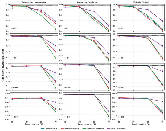
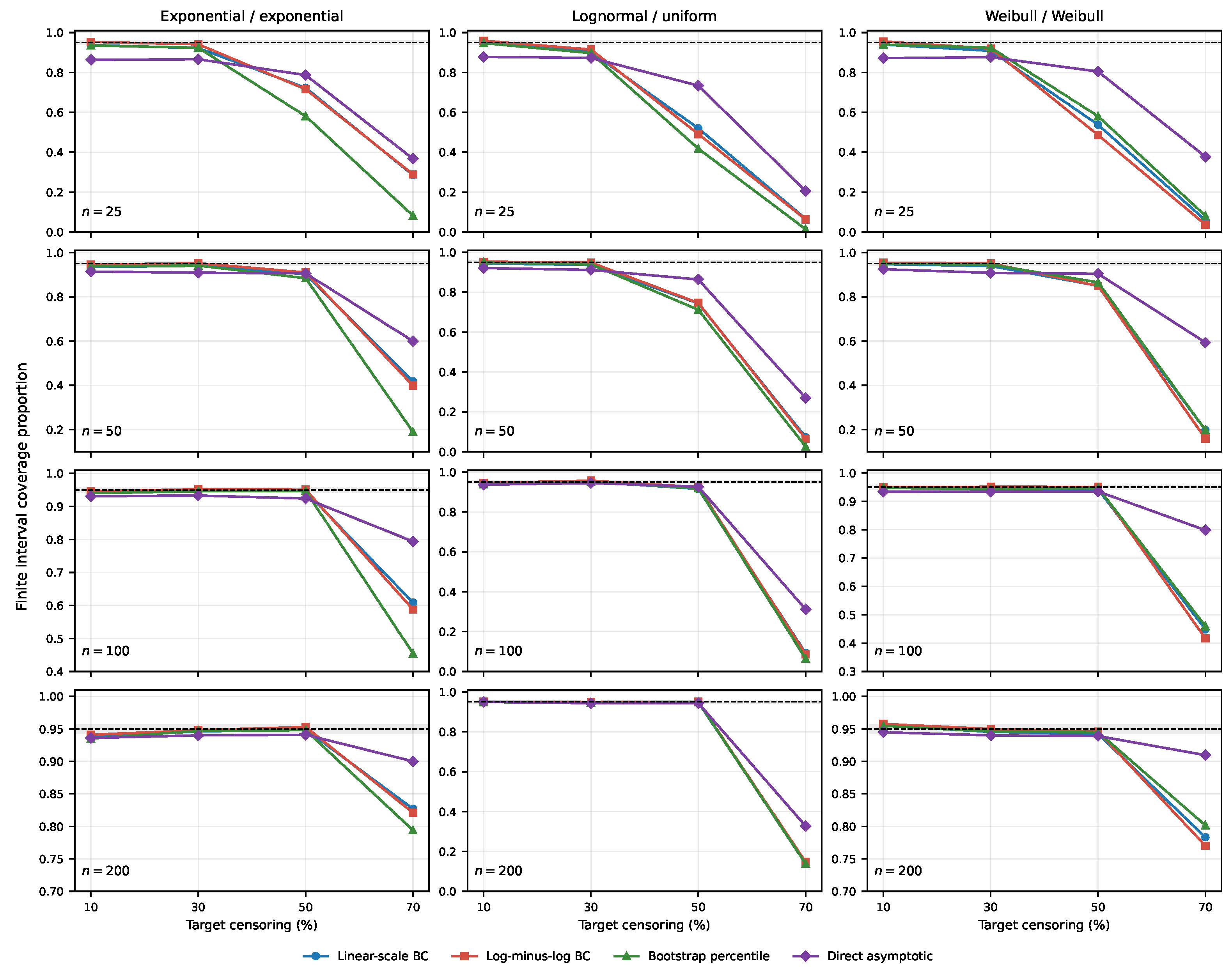
The empirical finite interval coverage probabilities are reported in Table 2, Table 3 and Table 4 and displayed in Figure 1. The results are very similar across the three models when censoring is mild and the sample size is reasonably large. Under Model 1, for example, the log-minus-log Brookmeyer–Crowley coverage probabilities for $n=100$ were 0.946, 0.952 and 0.951 at 10%, 30% and 50% censoring. The corresponding values under Model 2 were 0.946, 0.957 and 0.925. Under Model 3, they were 0.950, 0.951 and 0.951.

Table 2. Empirical finite interval coverage probabilities for exponential lifetimes with exponential censoring. The target coverage probability is 0.95; intervals without two finite endpoints count as noncoverage.

n	Censoring (%)	BC	LML	BP	AD
25	10	0.937	0.953	0.935	0.863
	30	0.922	0.941	0.924	0.866
	50	0.723	0.716	0.581	0.787
	70	0.285	0.289	0.082	0.367
50	10	0.935	0.946	0.938	0.914
	30	0.940	0.952	0.941	0.909
	50	0.902	0.910	0.884	0.906
	70	0.418	0.399	0.190	0.600
100	10	0.940	0.946	0.940	0.931
	30	0.946	0.952	0.946	0.933
	50	0.946	0.951	0.947	0.924
	70	0.609	0.588	0.455	0.794
200	10	0.938	0.941	0.935	0.936
	30	0.946	0.948	0.947	0.940
	50	0.949	0.953	0.948	0.941
	70	0.827	0.821	0.794	0.900

Table 3. Empirical finite-interval coverage probabilities for lognormal lifetimes with uniform censoring. The target coverage probability is 0.95; intervals without two finite endpoints count as noncoverage.

n	Censoring (%)	BC	LML	BP	AD
25	10	0.947	0.959	0.947	0.878
	30	0.902	0.915	0.897	0.873
	50	0.520	0.491	0.418	0.734
	70	0.066	0.063	0.014	0.205
50	10	0.944	0.953	0.949	0.921
	30	0.937	0.949	0.940	0.912
	50	0.744	0.746	0.712	0.864
	70	0.073	0.065	0.026	0.270
100	10	0.939	0.946	0.939	0.937
	30	0.951	0.957	0.950	0.945
	50	0.916	0.925	0.919	0.927
	70	0.093	0.087	0.065	0.312
200	10	0.949	0.951	0.949	0.950
	30	0.947	0.949	0.945	0.943
	50	0.947	0.951	0.949	0.944
	70	0.146	0.147	0.138	0.327

Table 4. Empirical finite-interval coverage probabilities for Weibull lifetimes with increasing hazard and Weibull censoring. The target coverage probability is 0.95; intervals without two finite endpoints count as noncoverage.

n	Censoring (%)	BC	LML	BP	AD
25	10	0.940	0.955	0.940	0.871
	30	0.908	0.920	0.924	0.877
	50	0.538	0.486	0.580	0.805
	70	0.059	0.037	0.081	0.378
50	10	0.947	0.954	0.950	0.925
	30	0.939	0.951	0.946	0.908
	50	0.850	0.850	0.865	0.905
	70	0.198	0.160	0.198	0.593
100	10	0.948	0.950	0.948	0.934
	30	0.943	0.951	0.943	0.934
	50	0.942	0.951	0.947	0.935
	70	0.449	0.417	0.460	0.798
200	10	0.955	0.958	0.955	0.945
	30	0.945	0.950	0.946	0.940
	50	0.942	0.946	0.945	0.939
	70	0.783	0.770	0.802	0.910

Figure 1. Empirical finite-interval coverage probabilities. The horizontal line represents the nominal 0.95 level and the narrow grey band represents approximate Monte Carlo variation around 0.95 for $R=5000$. Intervals without two finite endpoints count as noncoverage. The columns correspond to Models 1–3, the rows to the four sample sizes, and vertical scales vary by panel to make differences between procedures easier to see.

For 10% and 30% censoring, the linear-scale and log-minus-log Brookmeyer–Crowley intervals and the bootstrap interval generally produced coverage probabilities close to 0.95 once $n\ge 50$. The log-minus-log Brookmeyer–Crowley interval was often closest to the nominal level. The direct asymptotic interval performed less well in the smaller samples. For example, under Model 1 with $n=25$ and 10% censoring, its coverage was 0.863, compared with 0.937, 0.953 and 0.935 for the other three methods.

The effect of censoring becomes much more prominent at 50% censoring. Under Model 1, the procedures performed well for $n\ge 100$, but not for $n=25$. Under Model 2, to attain approximate nominal coverage at 50% censoring required a sample size close to 200. This difference arises because uniform censoring yields less follow-up in the upper tail of the lifetime distribution. Under Model 3, the first three procedures were already close to 0.95 at 50% censoring when $n=100$.

At 70% censoring, none of the procedures produced satisfactory coverage probabilities. In Model 1, increasing the sample size improved coverage, but even at $n=200$ the values ranged from 0.794 to 0.900. In Model 2, the coverage probability remained very low even when $n=200$. This is not primarily a failure of how the intervals were constructed. In that model, censoring occurs before time 12.50, which is only slightly beyond the true median of 10. Therefore, there is very little information available to estimate an upper confidence limit for the median. Model 3 also showed a pronounced finite-interval problem at 70% censoring. At $n=200$, the coverage probabilities were 0.783, 0.770, 0.802 and 0.910 for BC, LML, BP and AD, respectively.

4.2. Average Interval Lengths

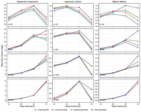
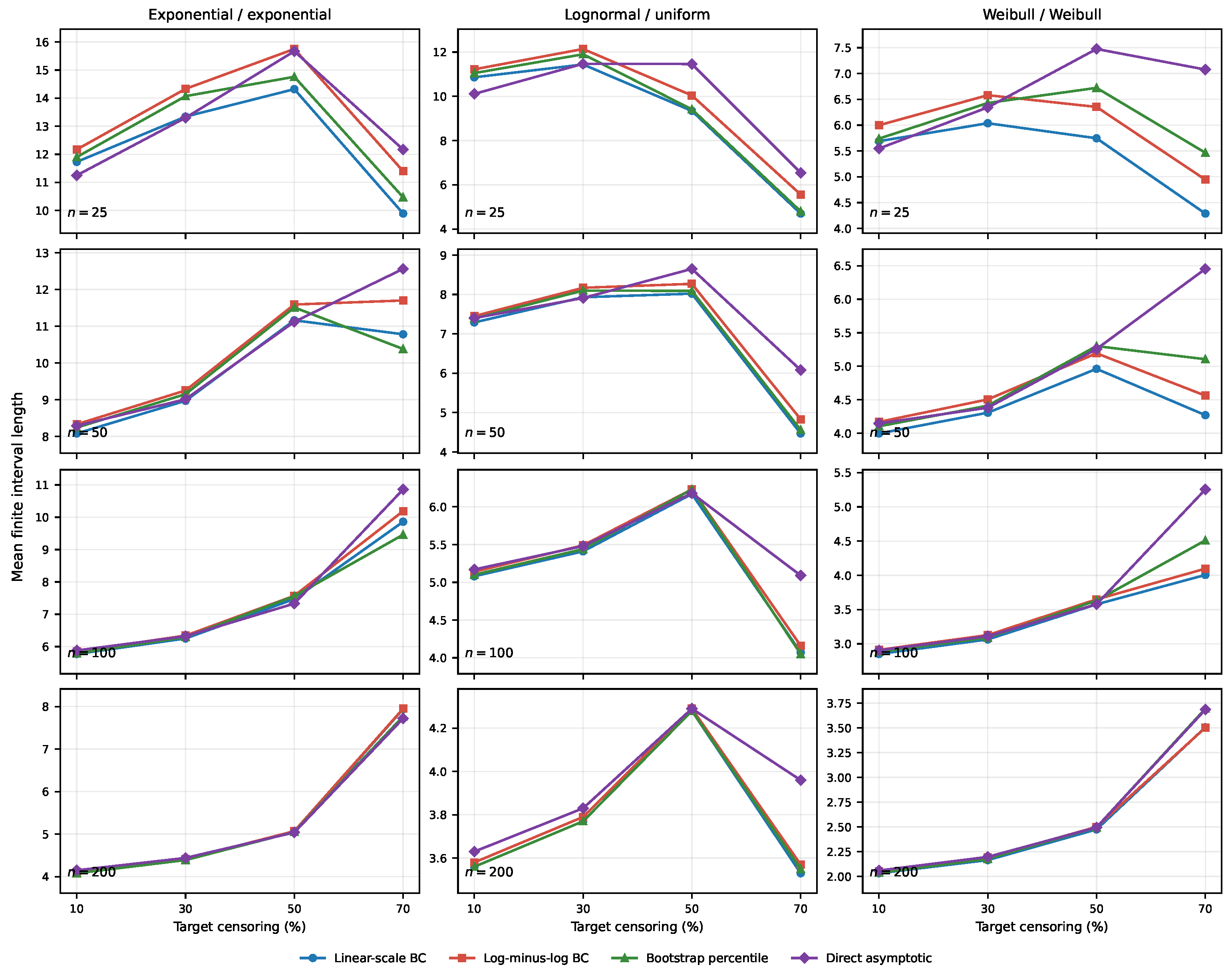
Mean interval lengths among finite intervals are reported in Table 5, Table 6 and Table 7 and displayed in Figure 2. In the settings where nearly all intervals were finite, the four methods produced broadly similar lengths. For example, under Model 1 with $n=100$ and 50% censoring, the mean lengths ranged from 7.33 for the direct asymptotic interval to 7.57 for the log-minus-log Brookmeyer–Crowley interval. Under Model 2 with $n=200$ and 50% censoring, all four means were approximately 4.3. Under Model 3 in the same setting, the four means were approximately 2.5.

Table 5. Mean interval lengths among finite intervals for exponential lifetimes with exponential censoring.

n	Censoring (%)	BC	LML	BP	AD
25	10	11.73	12.17	11.90	11.25
	30	13.34	14.33	14.07	13.30
	50	14.32	15.75	14.76	15.67
	70	9.89	11.40	10.47	12.17
50	10	8.08	8.33	8.24	8.29
	30	8.97	9.25	9.15	9.01
	50	11.16	11.59	11.51	11.12
	70	10.78	11.70	10.38	12.56
100	10	5.77	5.85	5.79	5.88
	30	6.25	6.34	6.29	6.32
	50	7.47	7.57	7.56	7.33
	70	9.86	10.19	9.46	10.86
200	10	4.08	4.11	4.08	4.15
	30	4.39	4.41	4.39	4.44
	50	5.05	5.07	5.05	5.04
	70	7.94	7.95	7.77	7.72

Table 6. Mean interval lengths among finite intervals for lognormal lifetimes with uniform censoring.

n	Censoring (%)	BC	LML	BP	AD
25	10	10.86	11.22	11.05	10.11
	30	11.44	12.14	11.90	11.47
	50	9.34	10.04	9.41	11.46
	70	4.70	5.56	4.80	6.54
50	10	7.29	7.45	7.39	7.40
	30	7.93	8.17	8.10	7.91
	50	8.02	8.27	8.09	8.65
	70	4.47	4.83	4.56	6.08
100	10	5.08	5.14	5.10	5.17
	30	5.41	5.49	5.44	5.48
	50	6.17	6.23	6.23	6.18
	70	4.07	4.16	4.05	5.09
200	10	3.56	3.58	3.56	3.63
	30	3.77	3.79	3.77	3.83
	50	4.28	4.29	4.28	4.29
	70	3.53	3.57	3.55	3.96

Table 7. Mean interval lengths among finite intervals for Weibull lifetimes with increasing hazard and Weibull censoring.

n	Censoring (%)	BC	LML	BP	AD
25	10	5.69	6.00	5.74	5.55
	30	6.04	6.58	6.43	6.34
	50	5.75	6.35	6.72	7.47
	70	4.29	4.94	5.47	7.08
50	10	4.00	4.17	4.10	4.15
	30	4.31	4.51	4.41	4.38
	50	4.96	5.19	5.30	5.26
	70	4.27	4.56	5.11	6.45
100	10	2.85	2.91	2.88	2.91
	30	3.06	3.13	3.09	3.11
	50	3.58	3.65	3.63	3.58
	70	4.01	4.10	4.51	5.25
200	10	2.03	2.05	2.04	2.06
	30	2.16	2.19	2.18	2.20
	50	2.47	2.50	2.49	2.49
	70	3.51	3.50	3.69	3.69

Figure 2. Mean interval lengths among replications in which both interval limits were finite. Shorter mean length is not necessarily better when the undefined rate is high. The columns correspond to Models 1–3, the rows to the four sample sizes, and vertical scales vary by panel.

Some average lengths decrease when censoring becomes very heavy. This should not be interpreted as better precision. This occurs because many difficult samples do not yield a finite upper limit and are therefore excluded from the length calculation. The remaining intervals come from the more “favourable” samples and are not representative of the full simulation scenario. Average length must therefore be considered together with coverage and the undefined rate.

4.3. Undefined Finite Intervals

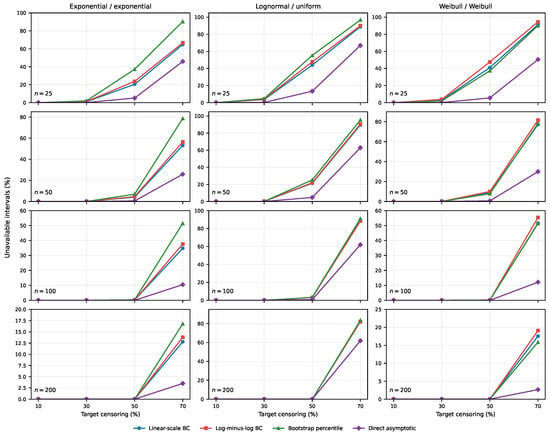
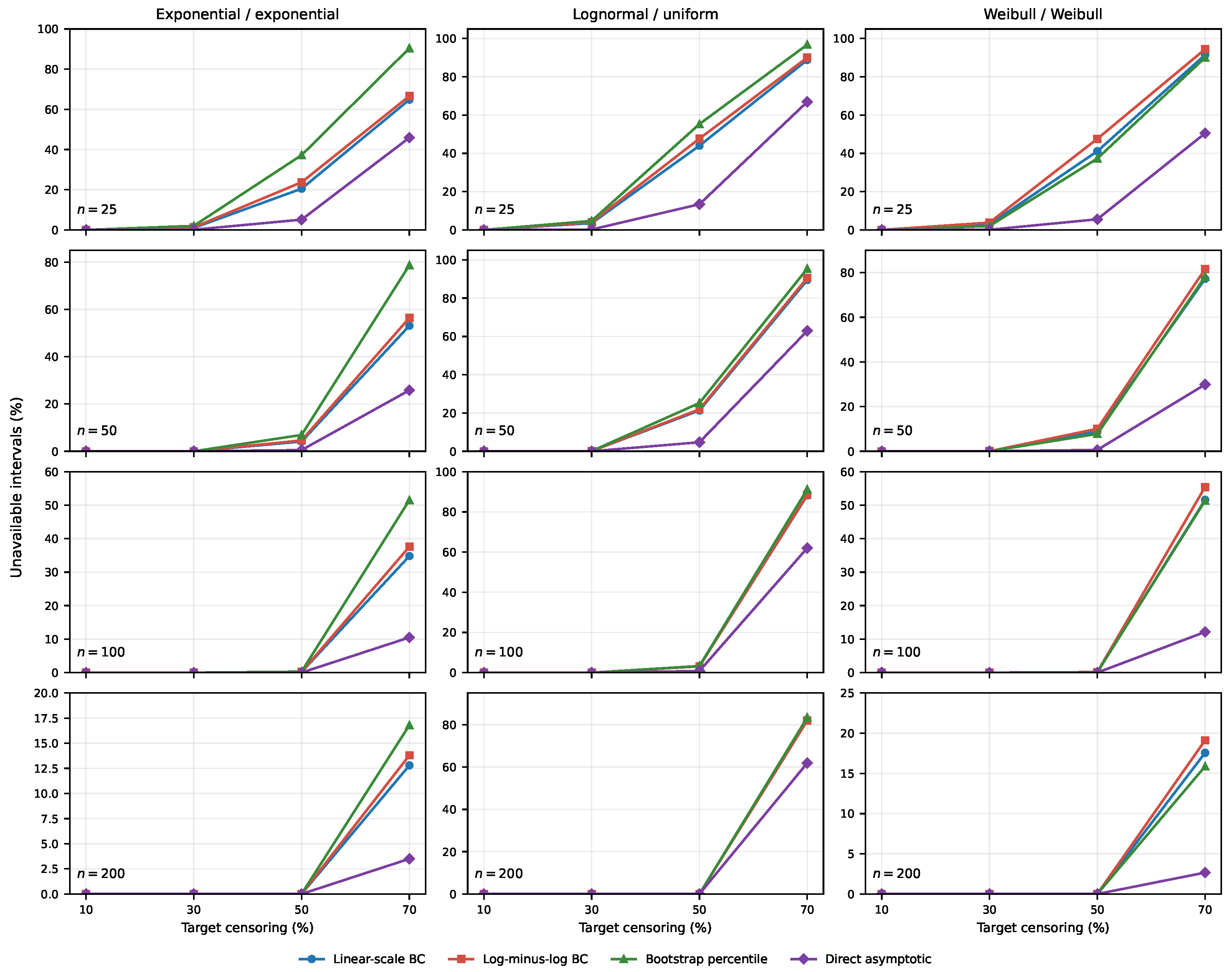
The undefined rates are reported in Table 8, Table 9 and Table 10 and displayed in Figure 3. With 10% censoring, finite intervals were obtained in basically every replication. The same was true at 30% censoring except for the smallest sample size.

Table 8. Percentage of replications in which a finite two-sided interval could not be obtained for exponential lifetimes with exponential censoring.

n	Censoring (%)	BC	LML	BP	AD
25	10	0.0	0.0	0.0	0.0
	30	1.0	1.3	2.0	0.1
	50	20.5	23.7	37.2	5.1
	70	64.8	66.6	90.4	45.9
50	10	0.0	0.0	0.0	0.0
	30	0.0	0.0	0.0	0.0
	50	4.1	4.6	6.9	0.5
	70	53.1	56.4	78.7	25.8
100	10	0.0	0.0	0.0	0.0
	30	0.0	0.0	0.0	0.0
	50	0.2	0.2	0.3	0.0
	70	34.8	37.6	51.5	10.5
200	10	0.0	0.0	0.0	0.0
	30	0.0	0.0	0.0	0.0
	50	0.0	0.0	0.0	0.0
	70	12.8	13.8	16.8	3.5

Table 9. Percentage of replications in which a finite two-sided interval could not be obtained for lognormal lifetimes with uniform censoring.

n	Censoring (%)	BC	LML	BP	AD
25	10	0.0	0.0	0.0	0.0
	30	3.5	4.0	4.7	0.2
	50	44.0	47.7	55.3	13.4
	70	88.8	90.0	96.8	66.9
50	10	0.0	0.0	0.0	0.0
	30	0.1	0.1	0.1	0.0
	50	21.3	21.9	25.2	4.7
	70	89.5	90.6	95.4	62.9
100	10	0.0	0.0	0.0	0.0
	30	0.0	0.0	0.0	0.0
	50	3.2	3.1	3.3	0.8
	70	88.2	88.5	91.2	62.0
200	10	0.0	0.0	0.0	0.0
	30	0.0	0.0	0.0	0.0
	50	0.0	0.0	0.0	0.0
	70	82.4	82.0	83.4	61.9

Table 10. Percentage of replications in which a finite two-sided interval could not be obtained for Weibull lifetimes with increasing hazard and Weibull censoring.

n	Censoring (%)	BC	LML	BP	AD
25	10	0.0	0.0	0.0	0.0
	30	2.8	3.8	2.0	0.1
	50	41.1	47.6	37.3	5.5
	70	91.4	94.4	90.0	50.5
50	10	0.0	0.0	0.0	0.0
	30	0.0	0.0	0.0	0.0
	50	8.8	10.1	7.8	0.6
	70	77.2	81.6	78.2	29.9
100	10	0.0	0.0	0.0	0.0
	30	0.0	0.0	0.0	0.0
	50	0.1	0.2	0.1	0.0
	70	51.6	55.4	51.3	12.1
200	10	0.0	0.0	0.0	0.0
	30	0.0	0.0	0.0	0.0
	50	0.0	0.0	0.0	0.0
	70	17.6	19.1	15.9	2.7

Figure 3. Percentage of replications in which a finite two-sided confidence interval could not be obtained. The columns correspond to Models 1–3, the rows to the four sample sizes, and vertical scales vary by panel.

At 50% censoring, sample size became important. Under Model 1 with $n=25$, the undefined rates were 20.5%, 23.7%, 37.2% and 5.1% for the linear-scale Brookmeyer–Crowley, log-minus-log Brookmeyer–Crowley, bootstrap and direct asymptotic intervals, respectively. These rates were close to zero when $n=200$. Under Model 2, the corresponding rates at $n=25$ were even higher, but again approached zero at $n=200$.

The picture at 70% censoring is different. Under Model 1, undefined rates decreased as the sample size increased, although they remained noticeable even at $n=200$. Under Model 2, more than 80% of the linear-scale and log-minus-log Brookmeyer–Crowley intervals and the bootstrap intervals were still unavailable at $n=200$. Increasing the sample size did not overcome the limited follow-up at the sample sizes considered here. Since ${\tau }_C=12.5>m=10$, the median remains theoretically identifiable, but considerably larger samples may be required when so little follow-up is available beyond it. Under Model 3, the corresponding unavailable rates at 70% censoring and $n=200$ were 17.6%, 19.1%, 15.9% and 2.7% for BC, LML, BP and AD, respectively. Thus, the unbounded Weibull censoring model improved markedly with increasing sample size, although finite endpoints were still not guaranteed under heavy censoring.

The direct asymptotic interval had fewer undefined intervals in the most difficult scenarios because it uses a symmetric normal approximation once the required sample quantiles are available. However, its coverage was still far below 0.95. A lower undefined rate does not make the direct interval reliable when its underlying approximation is poor.

4.4. Targeted Follow-Up and Sensitivity Results

The central role of follow-up is shown more directly in Table 11. Both scenarios use the same lognormal lifetime distribution, $n=200$ and approximately 70% censoring. The uniform censoring distribution ends at 12.50, whereas exponential censoring has unbounded support. With bounded follow-up, more than 82% of the BC, LML and BP intervals were unavailable. With unbounded follow-up, the corresponding rates were between 5.1% and 6.6%. The large difference at the same overall censoring percentage provides direct evidence that censoring percentage alone does not describe the information available for median inference.

Table 11. Comparison at $n=200$ for lognormal lifetimes with approximately 70% censoring but different follow-up support.

Procedure	Bounded Uniform Censoring		Unbounded Exponential Censoring
	CP	UIR (%)	CP	UIR (%)
Linear-scale BC	0.140	83.6	0.886	6.1
Log-minus-log BC	0.141	83.2	0.886	6.6
Bootstrap percentile	0.149	82.8	0.897	5.1
Direct asymptotic	0.331	62.0	0.926	0.8

Table 12 extends the difficult bounded-follow-up setting to $n=500$ and 1000. Although the unavailable rates of the BC, LML and BP intervals decreased substantially, reaching 30–34% at $n=1000$, a finite upper limit was still not guaranteed. Although $n=1000$ is already large for many applied survival studies, the censoring endpoint is only 25% beyond the true median in this setting. The continued unavailability of approximately one third of the intervals therefore shows that a large sample cannot fully compensate for very limited follow-up beyond the median. The direct asymptotic interval behaved differently: its density estimator requires the 60th percentile, while $F_T\left(12.50\right)\approx 0.588$. That percentile is beyond the observable endpoint, so increasing n cannot make the particular density estimator used here consistently available. This explains the direct interval’s 67.6% unavailable rate at $n=1000$.

Table 12. Large-sample extension for lognormal lifetimes with 70% bounded uniform censoring.

n	Source	CP				UIR (%)
		BC	LML	BP	AD	BC	LML	BP	AD
200	Main study	0.146	0.147	0.138	0.327	82.4	82.0	83.4	61.9
500	Extension	0.326	0.341	0.364	0.315	64.7	63.0	60.6	64.7
1000	Extension	0.633	0.646	0.673	0.290	34.3	32.8	30.2	67.6

Finally, Table 13 repeats the bootstrap calculation for the bounded lognormal setting with $n=200$ and 70% censoring. Increasing B from 1000 to 5000 changed CP by 0.004, UIR by 0.2 percentage points and mean finite length by 0.01. The conclusion that most bootstrap intervals are unavailable is therefore not an artefact of using $B=1000$. When the probability of an infinite bootstrap median is far above 2.5%, more resamples estimate that probability more precisely but do not create tail information that is absent from the sample.

Table 13. Sensitivity of the bootstrap percentile interval to the number of resamples for lognormal lifetimes with $n=200$, bounded uniform censoring and 70% censoring.

B	CP	UIR (%)	Mean Finite Length
1000	0.133	84.7	3.59
5000	0.129	84.9	3.58

4.5. Practical Interpretation

No procedure performed best in every setting, but the simulations suggest several practical recommendations.

First, in the scenarios with mild censoring and at least 50 observations, the linear-scale and log-minus-log Brookmeyer–Crowley intervals, as well as the bootstrap interval, all perform reasonably well. The log-minus-log Brookmeyer–Crowley interval is attractive as a routine choice because it is simple to calculate, does not require resampling and was often closest to the nominal coverage level. This recommendation is limited to the procedures and distributions studied here and is not a claim of universal superiority.

Second, with 50% censoring, the sample size and length of follow-up should be assessed carefully. A finite interval should not be taken for granted, particularly when n is small. The undefined rate should be reported whenever intervals are compared in a simulation study.

Third, the direct asymptotic interval should not be the routine default in small samples. It additionally requires estimation of the density at the median and showed noticeable undercoverage in the less demanding small-sample scenarios.

Finally, when 70% of the observations are censored, moving from one method to the other did not solve the information problem for the sample sizes considered. A longer follow-up, a substantially larger sample, or a different summary measure may be more appropriate.

For applied work, the following checks should be made before reporting a median and its confidence interval:

• verify that the Kaplan–Meier curve crosses 0.5 and that both confidence limits for the survival curve cross 0.5;
• inspect the number at risk around and beyond the estimated median;
• examine how far the observation period extends beyond the median rather than relying only on the overall censoring percentage;
• consider whether censoring is indeed independent of the event time, possibly after conditioning on observed characteristics; and
• if a finite upper limit is unavailable, report that fact and consider an earlier quantile or a restricted mean survival time instead of forcing a finite interval.

5. A Practical Illustration: Time to Closure of Software Issues

To illustrate the four procedures with real data, we considered the time taken to close issues in the scikit-learn software project. Scikit-learn is a widely used open-source machine-learning library [6]. Its public GitHub issue tracker records when each issue was opened and, when applicable, when it was closed. The example is useful because an issue that remains open at the end of the chosen follow-up period is naturally right censored.

The data were downloaded from the GitHub REST API on 14 August 2026 [28]. We first selected the 718 issues opened between 1 January and 31 December 2024. Pull requests were excluded by using the is:issue search qualifier. We also excluded 98 issues submitted by accounts whose names ended with bot, as well as one issue submitted by a non-user account. This left 619 issues for analysis. The automated-account rule was implemented by converting each login to lower case and testing whether it ended exactly in bot. The additional non-user record had creator type Organization.

For each issue, time was measured in days from its opening time to the closing time stored in the closed_at field of the downloaded snapshot. Each issue was followed for at most 365 days. An issue closed within 365 days was treated as an observed event. An issue still open, or closed only after 365 days, was censored at 365 days. This gave every issue the same maximum follow-up period. There were 462 observed closures and 157 censored issues, yielding a censoring percentage of 25.4%. Since GitHub issues can be reopened, the outcome should be interpreted as time to the closing time recorded in the frozen snapshot, rather than time to an irreversible resolution.

The censoring used here is administrative rather than loss to follow-up. At a chosen horizon $\tau$, every included issue has the same censoring time $C=\tau$; a fixed censoring time is independent of the underlying closure time. Issue difficulty, priority or type may certainly affect the event time and create heterogeneity in the marginal closure-time distribution, but these characteristics do not determine whether an issue receives 14, 30 or 365 days of follow-up in this analysis. The Kaplan–Meier curve should therefore be interpreted as a marginal description of the selected population of issues, not as a covariate-adjusted model for individual issues.

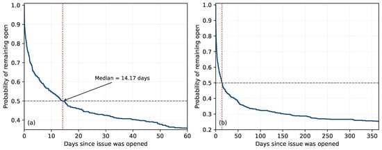
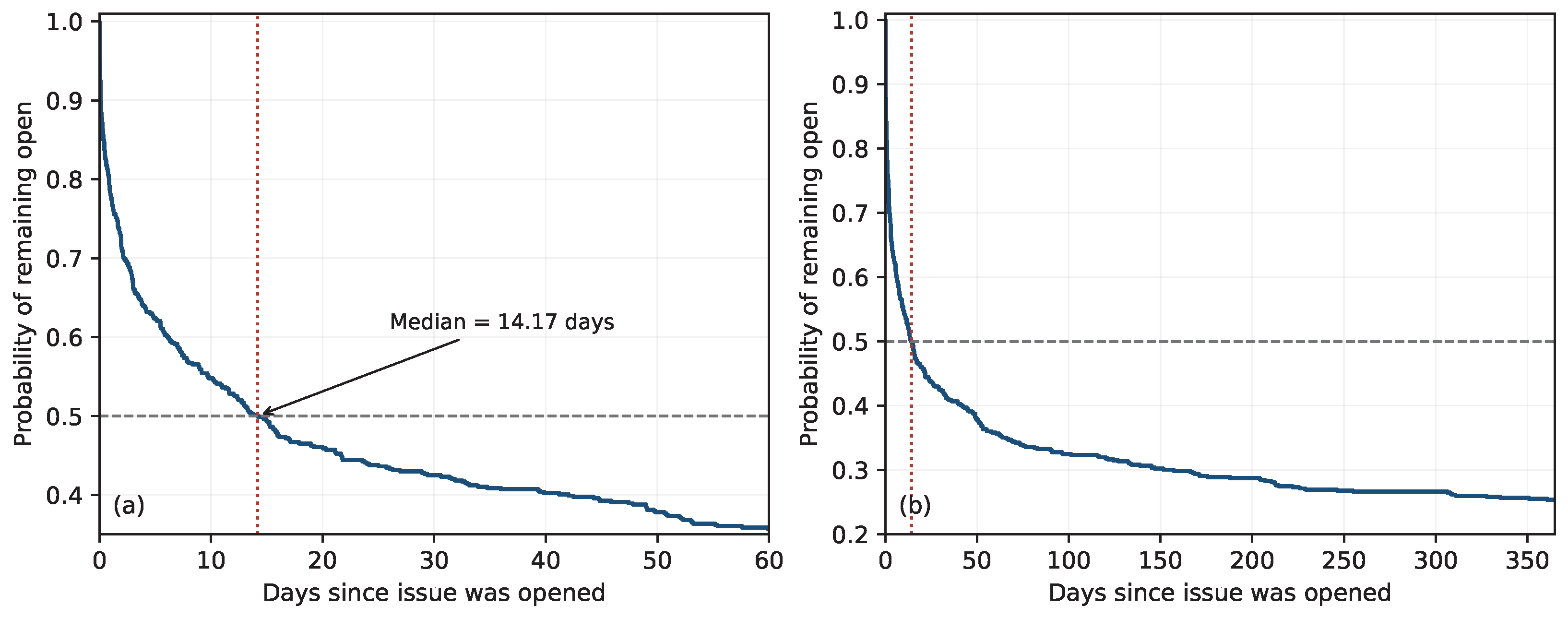
Figure 4 shows the Kaplan–Meier estimate of the probability that an issue remains open. The left panel gives a closer view of the first 60 days, while the right panel shows the complete 365-day follow-up. The estimated median time to closure was 14.17 days. In simple terms, approximately half of the issues had been closed by this time.

Figure 4. Kaplan–Meier estimate of the probability that a scikit-learn issue remains open: (a) the first 60 days and (b) the full 365-day follow-up. The dashed horizontal line is at 0.5 and the dotted vertical line marks the estimated median of 14.17 days.

For comparison, the ordinary median calculated from the 462 issues that closed within one year was only 4.79 days. That calculation completely discards the 157 censored issues and therefore gives an overly optimistic description of closure time. The Kaplan–Meier estimate retains the information that these issues remained open up to the censoring time. This simple difference shows why survival methods are useful for software project data.

Table 14 presents the four 95% confidence intervals. The bootstrap calculation used 100,000 resamples. The linear-scale and log-minus-log Brookmeyer–Crowley intervals and the bootstrap percentile interval were very similar. The direct asymptotic interval was wider. For this interval, the estimated 40th and 60th percentiles were 6.13 and 42.05 days, respectively. This illustrates the additional sensitivity and variability introduced by estimating the density in the direct method. The difference is not caused by skewness alone. The direct standard error is inversely proportional to the estimated density at the median. In this strongly right-skewed dataset, the wide spacing between the estimated 40th and 60th percentiles produces a small local density estimate and therefore a wider interval.

Table 14. Estimated 95% confidence intervals for the median time to closure, in days, using the 365-day follow-up.

Procedure	Lower Limit	Upper Limit
Linear-scale Brookmeyer–Crowley	10.96	19.22
Log-minus-log Brookmeyer–Crowley	10.83	19.22
Bootstrap percentile	10.96	19.22
Direct asymptotic	7.10	21.25

As a sensitivity analysis for the account exclusions, we repeated the 365-day calculation using all 718 records. The median changed from 14.17 to 9.29 days, and the linear-scale Brookmeyer–Crowley interval changed from $[10.96,19.22]$ to $[6.46,12.74]$. The difference indicates that the automated issues have a different closure-time distribution. The considerable change in the estimated median shows that the conclusions from this application are sensitive to the operational rule used to identify and exclude automated accounts. The analysis is therefore interpreted specifically for issues submitted by user accounts.

We also administratively censored the same issues after one week, two weeks and one month. The purpose was to show what is lost when the follow-up period is too short. Table 15 shows the result. After 7 days, only 255 of the 619 issues had been closed. At 14 days, 309 had been closed, which is still just fewer than half. The Kaplan–Meier curve therefore remained slightly above 0.5 and the median could not yet be estimated. With 30 days of follow-up, more than half of the issues had closed and the median could be estimated. Extending the follow-up to 365 days did not change the estimated median because the 0.5 crossing had already occurred at 14.17 days. To show how uncertainty changes, we also calculated all four confidence intervals after 7, 14, 30, 60, 90, 180 and 365 days of follow-up. The BC, LML and bootstrap intervals became finite after 30 days. The direct interval remained unavailable until 60 days because its estimated 60th percentile had not yet been observed. Further follow-up did not materially change the point estimate or the intervals.

Table 15. Effect of available follow-up on the estimated median and its 95% confidence intervals. A dash indicates that the required endpoint or quantile is unavailable.

Follow-Up (Days)	Median	Linear-Scale BC	Log-Minus-Log BC	Bootstrap	Direct Asymptotic
7	–	–	–	–	–
14	–	$[10.96,\infty )$	$[10.83,\infty )$	$[10.96,\infty )$	–
30	14.17	$[10.96,19.22]$	$[10.83,19.22]$	$[10.96,19.22]$	–
60	14.17	$[10.96,19.22]$	$[10.83,19.22]$	$[10.96,20.05]$	$[7.10,21.25]$
90	14.17	$[10.96,19.22]$	$[10.83,19.22]$	$[10.96,19.22]$	$[7.10,21.25]$
180	14.17	$[10.96,19.22]$	$[10.83,19.22]$	$[10.96,19.22]$	$[7.10,21.25]$
365	14.17	$[10.96,19.22]$	$[10.83,19.22]$	$[10.96,19.22]$	$[7.10,21.25]$

This illustration supports the main conclusion of the simulation study. With very short follow-up, the median is unavailable not because the wrong interval method was selected, but because fewer than half of the issues have experienced the event. Once the follow-up is long enough for the Kaplan–Meier curve to cross 0.5, the three inversion or resampling procedures give broadly similar answers.

6. Conclusions

We compared four confidence interval procedures for the median survival time across 48 simulation scenarios and illustrated their use with software-issue data. The simulations used three contrasting lifetime and censoring models, with 5000 Monte Carlo samples per scenario and 1000 resamples for each bootstrap interval. The practical illustration used time-to-closure data for 619 issues from the scikit-learn GitHub repository. Targeted follow-up, sample-size and bootstrap-sensitivity calculations were also used to examine the robustness of the main findings.

The linear-scale and log-minus-log Brookmeyer–Crowley intervals, as well as the bootstrap interval, yielded similar results when censoring was mild and the sample size was adequate. The log-minus-log Brookmeyer–Crowley interval generally provided a useful practical procedure and often achieved coverage closest to the nominal 95% level. This recommendation applies to the procedures and distributions studied here rather than universally. The direct asymptotic interval was less competitive in small samples because it requires the additional estimation of the density at the median. In the GitHub illustration, its wider interval also showed how the density-estimation step can matter in a strongly right-skewed data set. It can also be unavailable when the median itself is identifiable if the quantiles used to estimate that density lie beyond the observable follow-up period.

The most important finding concerns heavy censoring. When there was little follow-up beyond the median, finite upper confidence limits were frequently unavailable. This occurred especially under the lognormal/uniform model with 70% censoring, where the maximum censoring time was only slightly larger than the true median. Since the censoring endpoint still exceeded the true median, the median was theoretically identifiable; the difficulty was the small amount of finite-sample information available beyond it. The practical illustration made the same point more directly: with 14 days of follow-up, 309 of the 619 issues had closed and the Kaplan–Meier curve had not yet reached 0.5. The median could therefore not be estimated. With 30 days of follow-up, the median could be estimated as 14.17 days.

All simulations assume that the censoring time is independent of the event time. If we have dependent censoring, the Kaplan–Meier estimator and all four intervals can be biased or inconsistent. When dependence is explained by observed covariates, conditional modelling or inverse-probability-of-censoring weighting may be appropriate. Dependence through unobserved characteristics requires stronger modelling or sensitivity analysis. In the software example, censoring is instead fixed administratively at each selected horizon, although issue characteristics still create heterogeneity in the marginal closure-time distribution. Further work could study mixture lifetime distributions, covariate-adjusted medians, dependent censoring, subsampling and Bayesian bootstrap procedures.

The inversion and bootstrap ideas are not limited to the median and can be applied to another chosen survival quantile. More extreme quantiles require correspondingly longer follow-up, so the same identifiability and finite-endpoint checks remain necessary. When the Kaplan–Meier curve or its upper confidence limit does not reach the required probability level, changing the interval formula cannot replace unobserved information; an earlier quantile or restricted mean survival time may be more informative.

References

- Barlow, R.E.; Proschan, F. Statistical Theory of Reliability and Life Testing: Probability Models; Holt, Rinehart and Winston: New York, NY, USA, 1975. [Google Scholar]
- Blischke, W.R.; Murthy, D.N.P. Warranty Cost Analysis; Marcel Dekker: New York, NY, USA, 1994. [Google Scholar]
- Meeker, W.Q.; Escobar, L.A. Statistical Methods for Reliability Data; Wiley: New York, NY, USA, 1998. [Google Scholar]
- Fader, P.S.; Hardie, B.G.S. How to Project Customer Retention. J. Interact. Mark. 2007, 21, 76–90. [Google Scholar] [CrossRef] [Scilit]
- Lai, T.D.; Simmons, A.; Barnett, S.; Schneider, J.G.; Vasa, R. Comparative Analysis of Real Issues in Open-Source Machine Learning Projects. Empir. Softw. Eng. 2024, 29, 60. [Google Scholar] [CrossRef] [Scilit]
- Pedregosa, F.; Varoquaux, G.; Gramfort, A.; Michel, V.; Thirion, B.; Grisel, O.; Blondel, M.; Prettenhofer, P.; Weiss, R.; Dubourg, V.; et al. Scikit-learn: Machine Learning in Python. J. Mach. Learn. Res. 2011, 12, 2825–2830. [Google Scholar]
- Kaplan, E.L.; Meier, P. Nonparametric Estimation from Incomplete Observations. J. Am. Stat. Assoc. 1958, 53, 457–481. [Google Scholar] [CrossRef]
- Reid, N. Estimating the Median Survival Time. Biometrika 1981, 68, 601–608. [Google Scholar] [CrossRef]
- Brookmeyer, R.; Crowley, J. A Confidence Interval for the Median Survival Time. Biometrics 1982, 38, 29–41. [Google Scholar] [CrossRef] [Scilit] [PubMed]
- Emerson, J.D. Nonparametric Confidence Intervals for the Median in the Presence of Right Censoring. Biometrics 1982, 38, 17–27. [Google Scholar] [CrossRef] [Scilit] [PubMed]
- Slud, E.V.; Byar, D.P.; Green, S.B. A Comparison of Reflected Versus Test-Based Confidence Intervals for the Median Survival Time, Based on Censored Data. Biometrics 1984, 40, 587–600. [Google Scholar] [CrossRef] [Scilit] [PubMed]
- Strawderman, R.L.; Parzen, M.I.; Wells, M.T. Accurate Confidence Limits for Quantiles Under Random Censoring. Biometrics 1997, 53, 1399–1415. [Google Scholar] [CrossRef] [Scilit] [PubMed]
- Hutson, A.D. Bootstrap-Type Confidence Intervals for Quantiles of the Survival Distribution. Stat. Med. 2001, 20, 1693–1702. [Google Scholar] [CrossRef] [PubMed]
- Al Luhayb, A.S.M.; Coolen, F.P.A.; Coolen-Maturi, T. Smoothed Bootstrap for Right-Censored Data. Commun. Stat. Theory Methods 2024, 53, 4037–4061. [Google Scholar] [CrossRef] [Scilit]
- McGrath, S.; Yang, C.H.; Kimmelman, J.; Ozturk, O.; Steele, R.; Benedetti, A. Meta-Analysis of Median Survival Times with Inverse-Variance Weighting. Stat. Med. 2026, 45, e70533. [Google Scholar] [CrossRef] [Scilit] [PubMed]
- Barker, C. The Mean, Median, and Confidence Intervals of the Kaplan–Meier Survival Estimate—Computations and Applications. Am. Stat. 2009, 63, 78–80. [Google Scholar] [CrossRef] [Scilit]
- Aly, E.E.A.A.; Csőrgő, M.; Horváth, L. Strong Approximations of the Quantile Process of the Product-Limit Estimator. J. Multivar. Anal. 1985, 16, 185–210. [Google Scholar] [CrossRef] [Scilit][Green Version]
- Maller, R.A.; Zhou, X. Survival Analysis with Long-Term Survivors; Wiley: Chichester, UK, 1996. [Google Scholar]
- Efron, B.; Tibshirani, R.J. An Introduction to the Bootstrap; Chapman & Hall: New York, NY, USA, 1993. [Google Scholar]
- Davison, A.C.; Hinkley, D.V. Bootstrap Methods and Their Application; Cambridge University Press: Cambridge, UK, 1997. [Google Scholar] [CrossRef] [Scilit]
- Efron, B. Bootstrap Methods: Another Look at the Jackknife. Ann. Stat. 1979, 7, 1–26. [Google Scholar] [CrossRef] [Scilit]
- Efron, B. Censored Data and the Bootstrap. J. Am. Stat. Assoc. 1981, 76, 312–319. [Google Scholar] [CrossRef]
- Lo, A.Y. A Bayesian Bootstrap for Censored Data. Ann. Stat. 1993, 21, 100–123. [Google Scholar] [CrossRef] [Scilit]
- Arfè, A.; Muliere, P. A General Bayesian Bootstrap for Censored Data Based on the Beta–Stacy Process. J. Stat. Plan. Inference 2023, 222, 241–251. [Google Scholar] [CrossRef] [Scilit] [PubMed]
- Breslow, N.; Crowley, J. A Large Sample Study of the Life Table and Product-Limit Estimates Under Random Censorship. Ann. Stat. 1974, 2, 437–453. [Google Scholar] [CrossRef] [Scilit]
- Kalbfleisch, J.D.; Prentice, R.L. The Statistical Analysis of Failure Time Data, 2nd ed.; Wiley: Hoboken, NJ, USA, 2002. [Google Scholar] [CrossRef] [Scilit]
- Karrison, T. Confidence Intervals for Median Survival Times Under a Piecewise Exponential Model with Proportional Hazards Covariate Effects. Stat. Med. 1996, 15, 171–182. [Google Scholar] [CrossRef]
- GitHub. REST API Endpoints for Issues. 2026. Available online: https://docs.github.com/en/rest/issues/issues (accessed on 14 August 2026).
Disclaimer/Publisher’s Note: The statements, opinions and data contained in all publications are solely those of the individual author(s) and contributor(s) and not of MDPI and/or the editor(s). MDPI and/or the editor(s) disclaim responsibility for any injury to people or property resulting from any ideas, methods, instructions or products referred to in the content. |
© 2026 by the author. Licensee MDPI, Basel, Switzerland. This article is an open access article distributed under the terms and conditions of the Creative Commons Attribution (CC BY) license.