A Reinforcement-Learning-Based Hybrid SAC–LQR Framework for UR3e Multi-Waypoint Motion: System Design and Simulation-Based Evaluation

Abstract

Artificial intelligence is increasingly being investigated for robot motion generation, while conventional methods remain effective for deterministic waypoint tasks. This study evaluates reinforcement learning as a state-conditioned joint-reference-generation layer at runtime, not as a replacement for classical control. A hybrid soft actor–critic (SAC)–linear-quadratic regulator (LQR) framework was implemented for a four-phase UR3e waypoint task. The SAC policy generated bounded joint-reference increments every 50 ms, while six per-joint LQR loops tracked them every 5 ms. Across 50 randomised MATLAB/Simulink episodes, the framework achieved 96% full-task success upon first entry into a strict 5 mm place region, with a first-entry distance of $4.221\pm 0.381$ mm. Frozen-policy tests under broader initial configurations, unseen waypoints, model-parameter perturbations, SAC observation-vector noise, command delay, and external torque achieved 82–100% full-task success. Under the nominal protocol, matched offline-trajectory LQR and proportional–integral–derivative (PID) baselines and a conventional inverse-kinematics (IK)–trajectory–LQR baseline each achieved 100% task completion. Post-entry continuation showed that threshold-entry success did not yield sustained sub-5 mm placement over 0.5, 1.0, and 2.0 s dwell intervals. A separate MATLAB–Robot Operating System 2 (ROS 2) fake-hardware experiment characterised execution and communication latency, with a mean round-trip latency of 5.45 ms. It excluded the Simulink plant and LQR inner loops and, therefore, represents a pre-deployment controller-pipeline evaluation rather than validation of the complete architecture on a physical robot.

1. Introduction

Artificial intelligence (AI) and machine learning are increasingly integrated into modern manufacturing for planning, optimisation, perception, and decision making during robotic execution [1]. Learning-based methods, including reinforcement learning, are, therefore, being investigated as components of robotic systems that can respond to variations in task state and execution conditions [2,3,4].

Pick-and-place and multi-waypoint motion tasks provide structured benchmarks for studying motion generation, phase progression, and terminal positioning. Conventional programming, inverse kinematics (IK), and trajectory planning remain established and effective solutions when the workspace, target locations, and task sequence are known in advance [5,6]. Within this context, the present study investigates whether a pretrained soft actor–critic (SAC) policy can generate bounded, state-conditioned joint references at runtime during scheduler-controlled multi-waypoint progression, without executing an explicit per-episode IK and trajectory-planning procedure. The learned mechanism is evaluated alongside conventional planning and trajectory-tracking approaches under common task criteria.

The experimental scenario consists of a four-phase UR3e waypoint task. The labels pick, lift, cruise, and place denote successive end-effector waypoint phases managed by the scheduler. The experiments focus on motion generation, phase progression, and joint-level regulation. Gripper and object-contact dynamics, grasping and release, payload transfer, human–robot interaction, and collaboration-specific safety and collision-avoidance constraints are outside the evaluation scope. The task is, therefore, treated as a structured multi-waypoint motion problem rather than a complete physical pick-and-place operation.

SAC is applicable to continuous-control problems because its entropy-regularised formulation supports stochastic policy learning in continuous action spaces [7]. In the investigated Hybrid SAC–linear-quadratic regulator (LQR) architecture, the pretrained SAC policy generates bounded incremental joint-reference corrections every 50 ms. A scheduler manages waypoint-phase progression, while six per-joint LQR loops track the resulting references every 5 ms. This two-timescale structure separates state-conditioned reference generation and phase progression from faster local joint regulation.

The complete framework is implemented and evaluated in MATLAB/Simulink using randomised initial joint configurations. The evaluation includes matched offline-trajectory LQR and proportional–integral–derivative (PID) configurations, a conventional IK–trajectory–LQR baseline, frozen-policy robustness and generalisation tests, confidence intervals for task-success rates, and post-entry placement analysis.

A separate MATLAB–Robot Operating System 2 (ROS 2) experiment evaluates communication and controller-interface execution using the Universal Robots ROS 2 driver and the ros2_control fake-hardware backend. This adapted pipeline does not execute the Simulink plant or the six LQR inner loops and, therefore, does not represent the complete Hybrid SAC–LQR architecture. Validation through the complete Universal Robots simulator (URSim) controller backend and subsequent experiments on a physical UR3e remain future stages. The main contributions of this study are as follows:

• A Hybrid SAC–LQR architecture combining bounded incremental joint-space references, scheduler-based four-phase progression, and faster per-joint LQR regulation.
• A comparative simulation-based evaluation using conventional IK–trajectory–LQR and matched offline-trajectory LQR and PID configurations, together with robustness, generalisation, and post-entry placement analyses.
• A separately scoped MATLAB–ROS 2 fake-hardware evaluation of controller-interface execution and communication latency.

The remainder of the paper is organised as follows. Section 2, Section 3 and Section 4 present the related work, system description, and methodology. Section 5 describes the MATLAB–ROS 2 controller-pipeline evaluation, and Section 6 presents the results. Section 7 discusses the findings and presents the limitations and future research directions in dedicated subsections. Section 8 concludes the paper, while Appendix A provides supporting technical material.

2. Related Work

2.1. Artificial Intelligence, Reinforcement Learning, and Robotic Motion Generation

The growing use of artificial intelligence in manufacturing has extended the role of robotic systems beyond fixed automation towards perception-assisted and data-driven operation [1,8]. This development has motivated the use of learning-based components alongside established robot-control methods when task states or execution conditions vary [2,3,4].

Reinforcement learning has been widely studied in robotic manipulation because many tasks require state-conditioned actions during execution rather than the reproduction of a fixed precomputed trajectory or command sequence [2,3]. Pick-and-place is a common benchmark because it combines motion towards a pick region, progression through intermediate phases, and final placement with bounded error. Previous work on collaborative robot pick-and-place demonstrated reinforcement-learning-based execution in simulation and on a physical cobot, including changes in object position and manipulation of an unseen object [9]. Task decomposition is particularly relevant when a policy must progress through several waypoints rather than reach a single target.

Soft actor–critic is suited to continuous-control problems and uses an entropy-regularised objective to maintain exploration during training [7]. Kuo et al. [10] compared SAC with other reinforcement-learning algorithms for six-degree-of-freedom (6-DoF) robotic-arm point tracking and subsequently used SAC for obstacle avoidance in an object-picking task. In the present work, SAC generates bounded incremental joint-space references for a four-phase multi-waypoint task, while joint regulation is assigned to a separate control layer.

2.2. Classical Baselines and the Role of Reinforcement Learning

Classical robot programming, inverse kinematics, and trajectory planning remain the foundation of many industrial pick-and-place operations. When the workspace, object location, and target pose are known, a programmed sequence of Cartesian or joint-space commands can execute the task. Inverse kinematics maps the desired end-effector pose to feasible joint configurations, while trajectory planning defines the motion between them [5,6]. These methods are mature, interpretable, and well suited to structured industrial environments.

They, therefore, provide necessary reference cases for evaluating state-conditioned joint-reference generation. The present evaluation includes matched offline-trajectory LQR and PID configurations under the nominal protocol and a conventional IK–trajectory–LQR baseline under the nominal and applicable modified conditions. These comparisons separate the role of runtime reference generation from conventional trajectory generation and local tracking without presuming an advantage for either approach.

2.3. Hybrid Learning-Based and Model-Based Robot Control

A single learned policy that performs both task-level progression and low-level joint regulation must address distinct control functions. Layered learning-based and model-based approaches instead assign decision making or reference generation to the learned component and local tracking to a classical controller.

This principle has been investigated in robotic manipulation, where reinforcement learning has been combined with conventional low-level controllers to support task execution while reducing the burden placed on the learned policy [11]. Broader robot-learning research similarly identifies structured low-level execution as a practical system component [12]. Reward design is another relevant factor, and structured learning signals have been investigated in manipulator control to support policy training [13].

The architecture examined here follows this layered principle. SAC provides continuous, state-conditioned incremental joint-reference corrections [7], while LQR performs local regulation around the resulting references. Previous comparisons of PID and LQR, together with studies of LQR-based serial-manipulator control, support the use of model-based regulation for joint tracking and transient response [14,15]. The present evaluation also includes conventional trajectory-based and inverse-kinematics baselines to distinguish reference-generation behaviour from local regulation.

2.4. Simulation-Based Validation and ROS 2 Controller Pipelines

Simulation-based evaluation is an important stage in reinforcement-learning studies for robotic systems, particularly when policy training precedes execution through a different software or controller interface. Differences between training and deployment environments may arise from plant modelling, unmodelled dynamics, sensing and actuation effects, software timing, and communication behaviour [16,17]. Middleware-based execution also introduces interface and timing considerations related to message exchange and controller update rates [18,19].

ROS 2 provides a modular communication structure among control nodes, robot descriptions, simulated systems, and external software tools. This structure allows a trained decision pipeline to be examined outside its training environment before physical testing. ROS-based studies identify middleware integration as relevant to reproducible, deployment-oriented robot-learning workflows [19,20]. For Universal Robots platforms, MATLAB/Simulink–ROS 2 integration allows learning, simulation, and controller interfaces to operate across separate software environments.

Salgado Patrón and Vivas Albán [18] demonstrated MATLAB/Simulink communication with a simulated UR3e through ROS 2 Humble.

The MATLAB–ROS 2 stage reported here is limited to controller-pipeline execution using ROS 2 middleware, the Universal Robots ROS 2 driver, and a ros2_control fake-hardware interface. The fake-hardware backend introduces neither a second plant model nor additional robot dynamics. This stage, therefore, evaluates software integration, command timing, communication, and controller-interface execution rather than transfer across plant dynamics or validation on a physical robot.

2.5. Relation to Previous Work

The present manuscript builds on earlier studies by the authors on learning-based robotic manipulation, hybrid control, and simulation-based validation. Previous work examined a deep deterministic policy gradient (DDPG)–LQR architecture for an ABB IRB120 manipulator using RobotStudio and a Transmission Control Protocol/Internet Protocol (TCP/IP) interface [21]. A related study addressed trajectory optimisation for sequential manipulation using the Tower of Hanoi benchmark [22]. More recently, a MATLAB–Robot Operating System (ROS)–URSim pipeline was developed for UR3e sim-to-sim validation, focusing on software integration and policy execution [23].

The present study differs from the earlier UR3e pipeline work [23] by evaluating a Hybrid SAC–LQR architecture in MATLAB/Simulink with bounded incremental joint-reference generation, four-phase waypoint progression, and faster per-joint LQR regulation. It also includes matched LQR and PID configurations, a conventional IK–trajectory–LQR baseline, robustness and generalisation tests, and post-entry placement analysis. The MATLAB–ROS 2 fake-hardware controller-pipeline evaluation is reported separately from the complete simulation architecture. The contribution, therefore, lies in the architecture and its structured evaluation rather than in SAC, LQR, or ROS 2 integration alone.

3. System Description

This section describes the UR3e platform, the forward-kinematics implementation, the simplified per-joint simulation plant, and the four-phase multi-waypoint task used to evaluate the complete Hybrid SAC–LQR architecture in MATLAB R2024b and Simulink R2024b. The separately adapted MATLAB–ROS 2 controller pipeline is described in Section 5.

3.1. Robot Platform

The UR3e (Universal Robots A/S, Odense, Denmark) is a 6-DoF collaborative robotic manipulator with a nominal payload of 3 kg, a maximum reach of 500 mm, and a total mass of 11.2 kg, including the cabling and base [24]. Its compact structure is suitable for tabletop manipulation and structured multi-waypoint motion tasks.

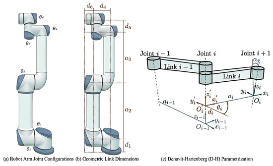
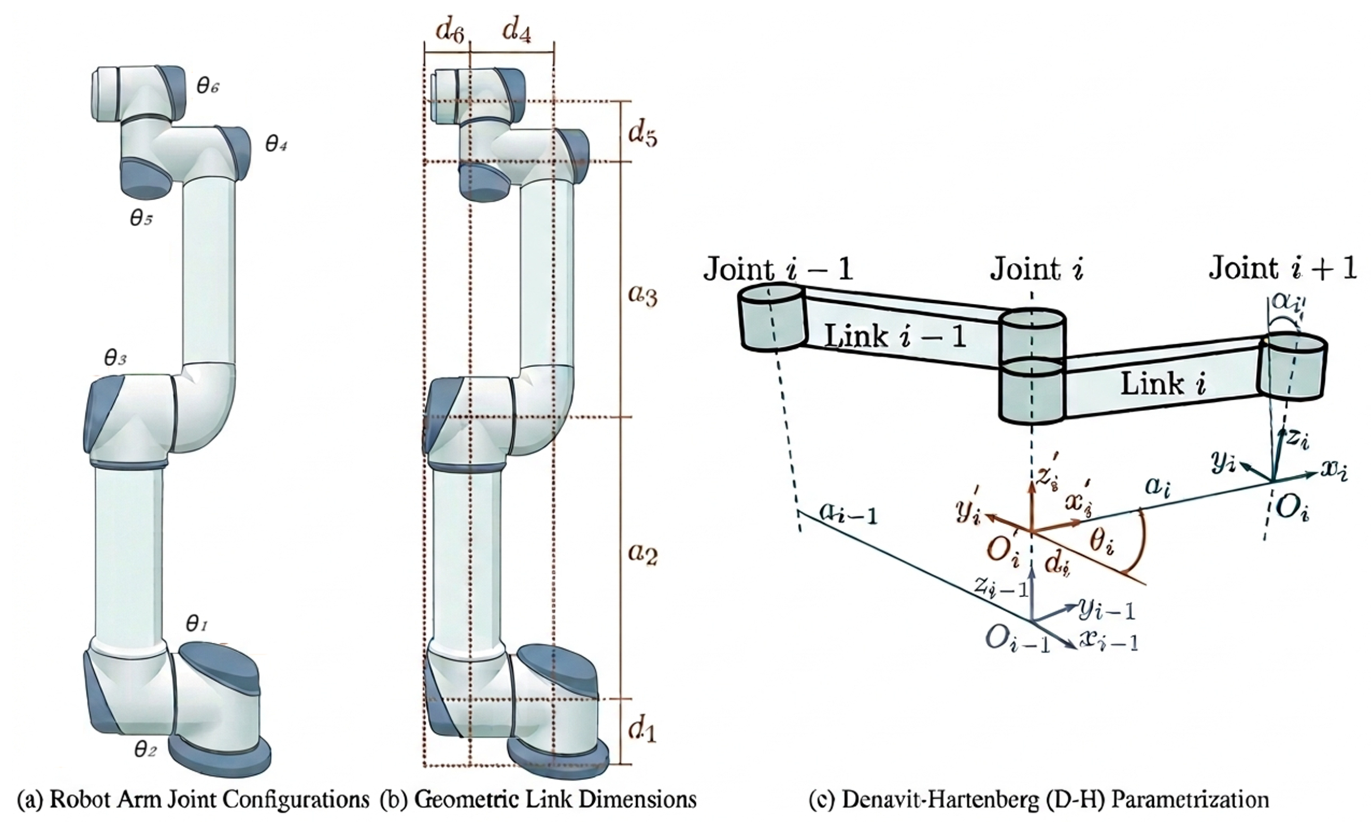
Figure 1 presents the robot geometry and the adopted Denavit–Hartenberg parametrisation. Panel (a) identifies the six joint angles ${\theta }_1,\dots ,{\theta }_6$, panel (b) shows the principal dimensions $a_2$, $a_3$, $d_1$, $d_4$, $d_5$, and $d_6$, and panel (c) illustrates the standard Denavit–Hartenberg frame convention. Panel (a) is adapted from the manufacturer’s documentation, while panels (b) and (c) are original.

Figure 1. UR3e robot geometry and kinematic notation: (a) joint-angle configuration; (b) principal geometric link dimensions; and (c) adopted Denavit–Hartenberg frame and parameter convention.

All six joints are represented in the MATLAB/Simulink model with software bounds of $\pm 2\pi$ rad. The adopted joint-speed limits are $\pi$ rad/s for joints 1–3 and $2\pi$ rad/s for joints 4–6, consistent with the rated limits. These bounds are enforced in the simulation model together with the bounded SAC-generated joint-reference increments described in Section 4.

3.2. Kinematic Model

The end-effector Cartesian position is computed at every simulation step using standard Denavit–Hartenberg (DH) forward kinematics. The homogeneous transformation between consecutive joint frames is

$${}^{i-1}T_i=\left[\begin{array}{cccc}\cos {\theta }_i& -\sin {\theta }_i\cos {\alpha }_i& \sin {\theta }_i\sin {\alpha }_i& a_i\cos {\theta }_i\\ \sin {\theta }_i& \cos {\theta }_i\cos {\alpha }_i& -\cos {\theta }_i\sin {\alpha }_i& a_i\sin {\theta }_i\\ 0& \sin {\alpha }_i& \cos {\alpha }_i& d_i\\ 0& 0& 0& 1\end{array}\right],$$

(1)

where ${\theta }_i$ is the joint angle, ${\alpha }_i$ is the link twist, $a_i$ is the link length, and $d_i$ is the joint offset. The complete base-to-end-effector transformation is

$${}^{0}T_6={}^{0}T_1{}^{1}T_2\cdots {}^{5}T_6,$$

(2)

and the end-effector position $\mathbf{p}\in {\mathbb{R}}^3$ is extracted from its translation component:

$$\mathbf{p}={}^{0}T_6(1:3,4).$$

(3)

The resulting position $\mathbf{p}$ is used by the SAC observation, reward calculation, and phase scheduler. The implemented DH parameters were obtained from the Unified Robot Description Format (URDF) model in the UR3e and cross-checked against the manufacturer specifications where available. Their values are listed in Table 1.

Table 1. UR3e Denavit–Hartenberg parameters used in the kinematic model, obtained from the URDF model and cross-checked against the manufacturer specifications where available.

Joint	${\mathit{\alpha }}_{\mathit{i}}$ (°)	${\mathit{a}}_{\mathit{i}}$ (mm)	${\mathit{d}}_{\mathit{i}}$ (mm)
1	$+90$	0	$151.85$
2	0	$-243.55$	0
3	0	$-213.20$	0
4	$+90$	0	$131.05$
5	$-90$	0	$85.35$
6	0	0	$92.10$

The implementation was verified at the zero-angle configuration $\mathit{\theta }=\mathbf{0}$, for which the forward-kinematics block produced $[-456.75,-223.15,66.50]$ mm. This result agreed to within 0.001 mm with a separately evaluated symbolic formulation using the same DH parameter set.

Forward kinematics is implemented in a MATLAB Function block using the %#codegen directive. The DH constants are defined locally to avoid workspace dependencies, and the block is evaluated at the fixed 5 ms simulation step.

3.3. Per-Joint Dynamics

In the MATLAB/Simulink evaluation, each joint is represented by a simplified third-order per-axis electromechanical plant. The model consists of an equivalent brushless direct-current (BLDC) actuator coupled to the joint through a high-ratio transmission with $G_R=1/101$, corresponding to 101 motor revolutions per joint revolution. It provides a structured simulation plant and is not intended to reproduce the complete coupled rigid-body dynamics of the physical UR3e. Gravity, Coriolis and centrifugal effects, inter-joint coupling, and nonlinear friction beyond the adopted viscous-damping term are not explicitly represented.

The physical state vector propagated in Simulink for joint j is

$${\mathbf{x}}_{p,j}={\left[\begin{array}{ccc}{\theta }_j& {\omega }_j& i_j\end{array}\right]}^{\mathsf{T}},$$

(4)

where ${\theta }_j$ is the joint angle, ${\omega }_j$ is the joint angular velocity, and $i_j$ is the motor-current state. The motor terminal voltage $u_j$ is the physical-plant input, and the continuous-time state equation is

$${\dot{\mathbf{x}}}_{p,j}=A_{p,j}{\mathbf{x}}_{p,j}+B_u{u}_j,$$

(5)

with

$$A_{p,j}=\left[\begin{array}{ccc}0& 1& 0\\ 0& -b_j/J_j& K_t/J_j\\ 0& -K_e/L& -R/L\end{array}\right],B_u=\left[\begin{array}{c}0\\ 0\\ 1/L\end{array}\right].$$

(6)

The joint reference ${\theta }_{\mathrm{ref},j}$ is supplied to the inner-loop controller and does not enter the physical plant as a separate state-space input. For LQR synthesis, the physical plant in Equations (4)–(6) was augmented with the design state

$$z_j={\int }_0^t\left({\theta }_{\mathrm{ref},j}-{\theta }_j\right)d\tau ,$$

(7)

giving the four-state synthesis vector

$${\mathbf{x}}_{d,j}={\left[\begin{array}{cccc}{z}_j& {\theta }_j& {\omega }_j& i_j\end{array}\right]}^{\mathsf{T}}.$$

(8)

This augmented state was used only to compute the LQR design gains. In the implemented Simulink realisation, $z_j$ is not accumulated as a feedback state. Instead, the magnitude of its design coefficient, $|k_{z,j}|$, is applied to the instantaneous tracking error $e_j={\theta }_{\mathrm{ref},j}-{\theta }_j$. Consequently, the implemented closed-loop pole calculation is based on the three-state plant ${\mathbf{x}}_{p,j}$, rather than the four-state augmented synthesis model. Section 4.1.3 gives the implemented feedback law and distinguishes it from the synthesis formulation.

A common representative electromechanical parameter set is used for the six per-axis actuator models. These motor-level constants are simulation parameters and are not presented as manufacturer-identified UR3e actuator parameters. Table 2 lists the values.

Table 2. Representative electrical and electromechanical parameters used in the simplified per-joint simulation model. The parameter set is common to all six per-axis models and is not presented as a manufacturer-identified UR3e actuator parameter set.

Symbol	Quantity	Value	Unit
$K_t$	Motor torque constant	$0.0437$	N·m/A
$K_e$	Back electromotive-force constant	$0.0437$	V·s/rad
R	Armature resistance	$0.50$	$\mathrm{\Omega }$
L	Armature inductance	$1.0\times {10}^{-3}$	H
$I_m$	Rotor inertia	$5.1\times {10}^{-5}$	kg·m2
$G_R$	Gear reduction factor	$1/101$	–
$V_{\max }$	Voltage saturation	$\pm 48$	V

The mechanical term $J_j$ is an approximate effective per-joint inertia used in the simplified control model. It combines the rotor-inertia term reflected through the transmission with selected diagonal inertia components from the UR3e URDF model:

$$J_j={\displaystyle \frac{I_m}{G_R^2}}+{\displaystyle \sum _{k=j}^6}{I}_{\mathrm{link},k}.$$

(9)

Here, $I_{\mathrm{link},k}$ denotes the selected diagonal component of the URDF inertia tensor associated with link k. The downstream-link terms are accumulated as a scalar per-axis approximation. Equation (9) is not a complete rigid-body inertia derivation involving transformed inertia tensors and parallel-axis terms. It instead defines the effective inertia values used consistently in the per-joint simulation and LQR design.

For the adopted parameters, the reflected rotor term is

$${\displaystyle \frac{I_m}{G_R^2}}\approx 0.5203\mathrm{kg}·{\mathrm{m}}^2,$$

(10)

and, therefore, dominates the effective per-joint inertia. The URDF-derived link components provide smaller joint-dependent adjustments. Table 3 lists the link masses, selected inertia components, effective inertias, and viscous damping coefficients.

Table 3. Per-joint mechanical parameters used in the simplified inner-loop control model. Link masses $m_j$ and selected diagonal inertia components $I_{\mathrm{link},j}$ are obtained from the UR3e URDF model, while the effective per-joint inertias $J_j$ are computed using Equation (9). The viscous damping coefficients $b_j$ are empirically selected simulation parameters and are not identified from physical UR3e measurements.

Joint j	${\mathit{m}}_{\mathit{j}}$ (kg)	${\mathit{I}}_{\mathbf{link},\mathit{j}}$ (kg·m2)	${\mathit{J}}_{\mathit{j}}$ (kg·m2)	${\mathit{b}}_{\mathit{j}}$ (N·m·s)
1	2.000	0.00562	0.5586	0.55
2	3.420	0.02173	0.5530	0.50
3	1.260	0.00654	0.5313	0.40
4	0.800	0.00208	0.5247	0.25
5	0.800	0.00225	0.5226	0.20
6	0.350	0.00014	0.5204	0.17

The motor terminal voltage $u_j$ is saturated at $\pm V_{\max }=\pm 48$ V before entering the actuator model. Joint angular velocity is software-limited to $\pm \pi$ rad/s for joints 1–3 and $\pm 2\pi$ rad/s for joints 4–6. Both saturation mechanisms are implemented inside the Simulink plant. The per-axis voltage-saturation duty cycle is reported as an evaluation metric in Section 6.

The matrices $A_{p,j}$ and $B_u$, therefore, define the simplified physical per-axis plant propagated in MATLAB/Simulink. Its purpose is to support structured joint-level control evaluation within the hybrid architecture, rather than to provide a physically identified model of the complete UR3e dynamics.

3.4. Task Definition

The task is defined as a four-phase sequence of Cartesian waypoints expressed in the robot base frame. The labels pick, lift, cruise, and place identify the successive phases managed by the scheduler. Gripper and object-contact dynamics, grasping and release, payload transfer, human–robot interaction, and collaboration-specific safety logic are outside the evaluation scope.

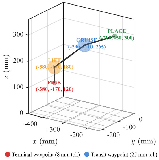
The pick and place waypoints define the first and final phases and use the tighter scheduler tolerance. The lift and cruise waypoints are intermediate phases and use a wider crossing tolerance because the corresponding regions need only be entered before the scheduler advances. Table 4 lists the Cartesian coordinates and scheduler tolerances.

Table 4. Cartesian waypoints and scheduler tolerances. The pick and place waypoints use an 8 mm tolerance, whereas lift and cruise use a 25 mm crossing tolerance.

Phase $\mathit{\varphi }$	Waypoint	x (mm)	y (mm)	z (mm)	Tolerance ${\mathit{\tau }}_{\mathit{\varphi }}$ (mm)
1	pick	$-380$	$-170$	120	8
2	lift	$-380$	$-170$	180	25
3	cruise	$-290$	$-110$	265	25
4	place	$-200$	$-50$	300	8

These coordinates define the nominal training and evaluation task. The shifted-waypoint configuration used in the generalisation test is specified separately in the experimental protocol. The waypoint heights increase monotonically across the four phases:

$$120\to 180\to 265\to 300\mathrm{mm}.$$

(11)

This vertical progression is an adopted curriculum choice that avoids an ascending–descending reversal before the terminal phase. The phase scheduler and curriculum rationale are described in Section 4.

The pick and place targets differ in Cartesian position and height and, therefore, require coordinated joint motion through the complete four-phase sequence. The strict success criterion reported in Section 6 requires first entry within 5 mm of the place waypoint. This criterion is tighter than the 8 mm scheduler tolerance. The wider scheduler zone supports phase progression during training, whereas the 5 mm criterion provides a stricter terminal evaluation condition. Threshold-entry success and post-entry placement behaviour are reported separately in Section 6.

4. Hybrid SAC–LQR Methodology

This section describes the two-timescale Hybrid SAC–LQR architecture, including the SAC observation and action interfaces, the implemented per-joint LQR regulation, the phase scheduler, reward design, and the MATLAB/Simulink experimental protocols. The numerical settings reported below define the configuration used in the simulation experiments.

4.1. Hybrid Architecture

4.1.1. Overview

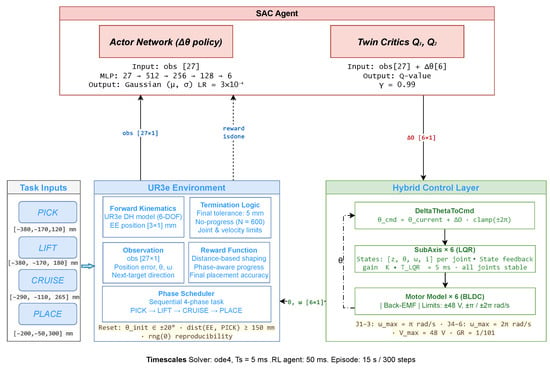
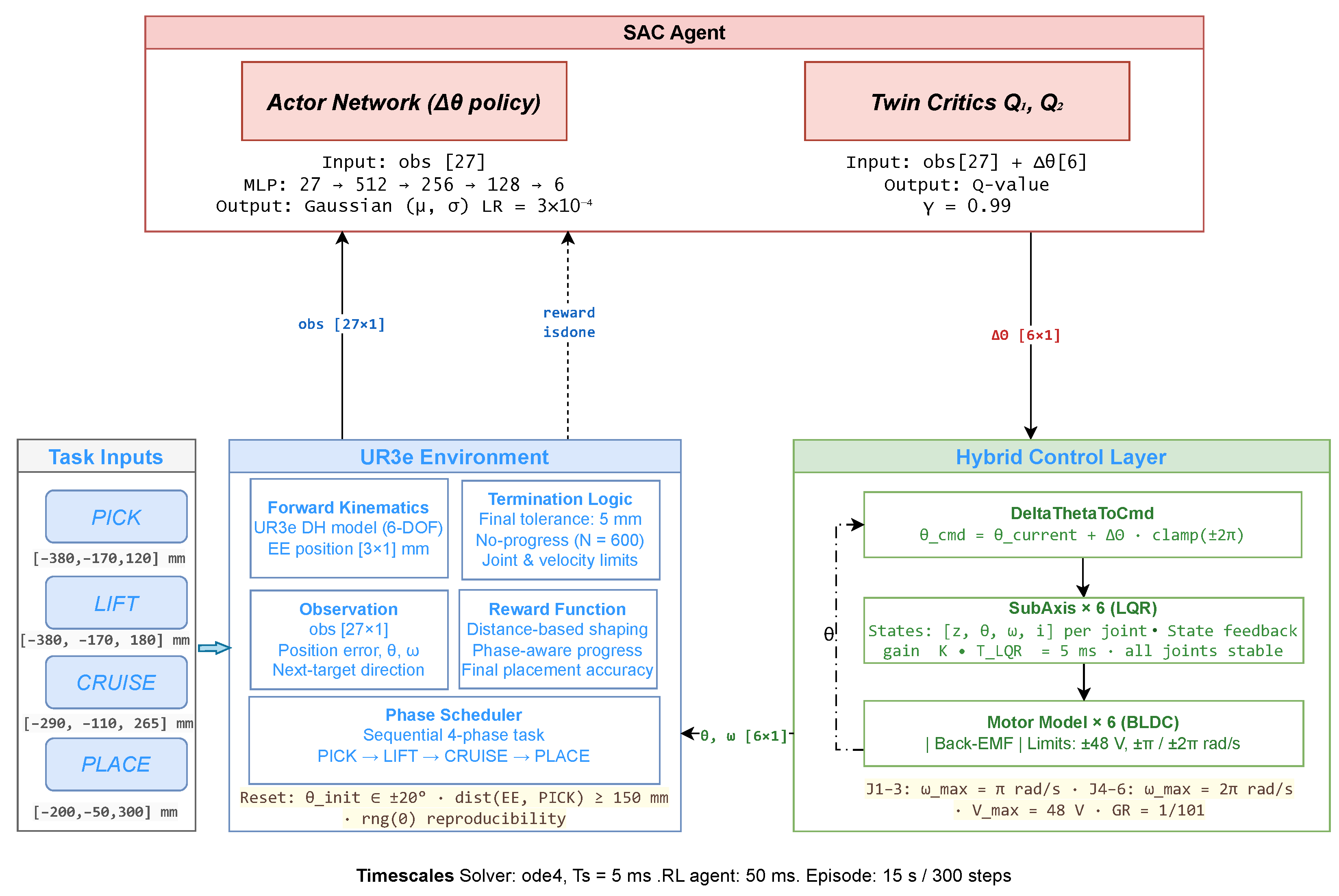
The architecture separates state-conditioned joint-reference generation from faster local joint regulation. The SAC outer loop generates bounded incremental joint-space corrections, while six independent per-joint LQR loops track the resulting references. Figure 2 shows the signal flow among the SAC agent, joint-reference conversion, LQR controllers, simplified UR3e plant, phase scheduler, observation block, and reward function.

Figure 2. Hybrid SAC–LQR control architecture for the four-phase UR3e multi-waypoint task.

The SAC outer loop generates $\Delta \mathit{\theta }\in {\mathbb{R}}^6$ every $T_{\mathrm{SAC}}=50$ ms. The joint-reference conversion block combines this correction with the current joint state to produce the absolute reference ${\mathit{\theta }}_{\mathrm{ref}}$. The six LQR loops track this reference at $T_{\mathrm{sim}}=5$ ms. Joint angles and velocities returned by the plant are used for inner-loop feedback and SAC observation construction, while the scheduler supplies the active and next Cartesian waypoints.

An agent step denotes one SAC decision interval, whereas a simulation step denotes one fixed-step plant-integration interval. Each SAC action is, therefore, held over ten simulation steps. A 15 s episode contains 300 agent decisions and 3000 simulation steps.

4.1.2. SAC Outer Loop

Action

The SAC action at decision step k is the six-component joint correction $\Delta {\mathit{\theta }}_k\in {\mathbb{R}}^6$. Each component is bounded according to the adopted joint-speed limit:

$$|\Delta {\theta }_{k,j}|\le T_{\mathrm{SAC}}{\omega }_{\max ,j},$$

(12)

where $T_{\mathrm{SAC}}=50$ ms. The resulting bounds are $0.1571$ rad for joints 1–3 and $0.3142$ rad for joints 4–6. These bounds constrain the reference increment generated during one SAC decision interval; they do not constrain the inner-loop voltage directly or preclude voltage saturation.

Observation

A 27-dimensional observation vector is constructed every 50 ms. Table 5 gives its components and scaling.

Table 5. Structure of the 27-dimensional SAC observation vector.

Components	Symbol	Expression	Meaning
1–3	${\mathbf{e}}_{\mathrm{near}}$	$({\mathbf{p}}_{\mathrm{target}}-\mathbf{p})/100$	Near-field Cartesian error
4–6	${\mathbf{e}}_{\mathrm{far}}$	$({\mathbf{p}}_{\mathrm{target}}-\mathbf{p})/300$	Far-field Cartesian error
7–9	${\mathbf{e}}_{\mathrm{next}}$	$({\mathbf{p}}_{\mathrm{next}}-\mathbf{p})/300$	Direction to the next waypoint
10–15	$\sin \left(\mathit{\theta }\right)$	$\sin \left({\theta }_{1\dots 6}\right)$	Joint-angle sines
16–21	$\cos \left(\mathit{\theta }\right)$	$\cos \left({\theta }_{1\dots 6}\right)$	Joint-angle cosines
22–27	${\mathit{\omega }}_{\mathrm{sc}}$	${\omega }_j/{\omega }_{\max ,j}$	Normalised joint velocities

Here, $\mathbf{p}$ is the current end-effector position, ${\mathbf{p}}_{\mathrm{target}}$ is the active waypoint, and ${\mathbf{p}}_{\mathrm{next}}$ is the subsequent waypoint. The Cartesian error terms and normalised velocities are clipped to $[-1,1]$. The two active-waypoint error scales provide near- and far-field position information, while ${\mathbf{e}}_{\mathrm{next}}$ supplies the direction of the subsequent phase. Joint angles are represented using sine and cosine components to avoid discontinuities at angular wrapping boundaries.

Network Architecture

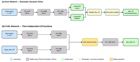
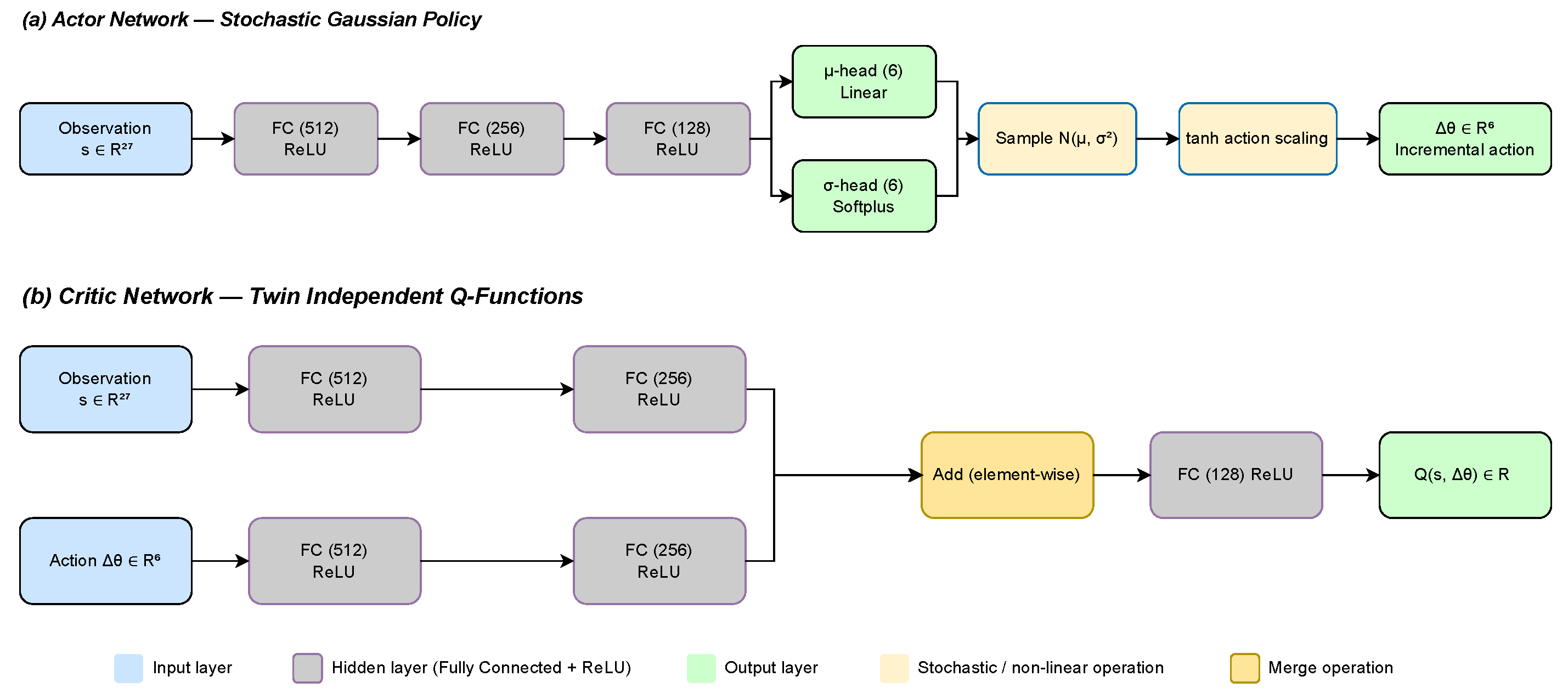
The SAC agent comprises a stochastic actor and two independent Q-value networks. The actor processes the 27-dimensional observation through three fully connected hidden layers containing 512, 256, and 128 units, respectively, with rectified linear unit (ReLU) activations. Two six-component output heads represent the Gaussian-policy mean and a Softplus-mapped standard deviation.

Each critic contains separate observation and action branches, both using fully connected layers of 512 and 256 units. Their outputs are combined through element-wise addition and passed through a 128-unit hidden layer to produce a scalar Q-value. During policy improvement, the smaller of the two critic estimates is used to reduce overestimation bias [25].

Figure 3 illustrates the adopted actor and critic structures.

Figure 3. SAC network architectures: (a) stochastic Gaussian actor and (b) one of the two independent Q-value networks.

Table 6 lists the SAC training and optimiser hyperparameters.

Table 6. SAC training and optimiser hyperparameters.

Parameter	Value	Parameter	Value
Discount factor $\gamma$	$0.99$	Actor learning rate	$3\times {10}^{-4}$
Target smoothing $\tau$	$1\times {10}^{-3}$	Critic learning rate	$3\times {10}^{-4}$
Mini-batch size	256	Gradient clipping threshold	$1.0$
Replay buffer length	$3\times {10}^6$	Entropy learning rate	$1\times {10}^{-5}$
Initial entropy weight ${\alpha }_0$	$0.01$	Target entropy	$-n_{\mathrm{act}}=-6$

4.1.3. LQR Inner-Loop Controller

For each joint, the three-state physical plant introduced in Section 3.3 was augmented for LQR gain synthesis using the design-only integral state in Equation (7). The resulting synthesis state vector is

$${\mathbf{x}}_{d,j}={\left[\begin{array}{cccc}{z}_j& {\theta }_j& {\omega }_j& i_j\end{array}\right]}^{\mathsf{T}}.$$

(13)

For regulation about a fixed reference, the augmented synthesis matrices are

$$A_{d,j}=\left[\begin{array}{cccc}0& -1& 0& 0\\ 0& 0& 1& 0\\ 0& 0& -b_j/J_j& K_t/J_j\\ 0& 0& -K_e/L& -R/L\end{array}\right],B_d=\left[\begin{array}{c}0\\ 0\\ 0\\ 1/L\end{array}\right].$$

(14)

The quadratic synthesis cost is

$${\mathcal{J}}_j={\int }_0^{\infty }\left({\mathbf{x}}_{d,j}^{\mathsf{T}}Q{\mathbf{x}}_{d,j}+u_j^{\mathsf{T}}{R}_{\mathrm{LQR}}{u}_j\right)dt,$$

(15)

with

$$Q=\mathrm{diag}(50,200,5,0.1),R_{\mathrm{LQR}}=0.1.$$

(16)

Solving the Riccati equation for $(A_{d,j},B_d)$ gives

$${\mathbf{K}}_{d,j}=\left[\begin{array}{cccc}{k}_{z,j}& k_{\theta ,j}& k_{\omega ,j}& k_{i,j}\end{array}\right].$$

(17)

These coefficients define the LQR synthesis result but are not applied as direct four-state feedback in the Simulink implementation. In particular, $z_j$ is not accumulated in the implemented controller. Instead, the magnitude of its synthesis coefficient is applied directly to the instantaneous tracking error

$$e_j={\theta }_{\mathrm{ref},j}-{\theta }_j.$$

(18)

The implemented voltage command for joint j is

$$u_j={\mathrm{sat}}_{\pm 48\mathrm{V}}\left(|k_{z,j}|e_j-k_{\theta ,j}{T}_{\mathrm{sim}}{\theta }_j-k_{\omega ,j}{\displaystyle \frac{{\omega }_j}{{\omega }_{\max ,j}}}-k_{i,j}{\displaystyle \frac{i_j}{I_{\max }}}\right),$$

(19)

where $T_{\mathrm{sim}}=0.005$ s, $I_{\max }=V_{\max }/R=96$ A, and ${\omega }_{\max ,j}$ is the adopted joint-speed limit: $\pi$ rad/s for joints 1–3 and $2\pi$ rad/s for joints 4–6.

Expanding $e_j={\theta }_{\mathrm{ref},j}-{\theta }_j$ gives the equivalent three-state representation

$$u_j={\mathrm{sat}}_{\pm 48\mathrm{V}}\left(k_{\mathrm{ref},j}{\theta }_{\mathrm{ref},j}-{\mathbf{K}}_{x,\mathrm{impl},j}{\mathbf{x}}_{p,j}\right),$$

(20)

where

$$k_{\mathrm{ref},j}=\left|k_{z,j}\right|,$$

(21)

and

$${\mathbf{K}}_{x,\mathrm{impl},j}=\left[\begin{array}{ccc}|k_{z,j}|+k_{\theta ,j}{T}_{\mathrm{sim}}& {\displaystyle \frac{k_{\omega ,j}}{{\omega }_{\max ,j}}}& {\displaystyle \frac{k_{i,j}}{I_{\max }}}\end{array}\right].$$

(22)

Thus, the term LQR in the Hybrid SAC–LQR designation refers to a local regulator whose coefficients are obtained from the augmented LQR synthesis procedure, while the implemented Simulink controller uses the equivalent three-state feedback form in Equation (20). For all six joints,

$$k_{\mathrm{ref},j}=\left|k_{z,j}\right|=22.3607.$$

(23)

Table 7 reports the synthesis gains, their equivalent implemented three-state values, and the corresponding nominal closed-loop poles.

Table 7. LQR synthesis gains and implemented closed-loop characteristics.

Joint	${\mathit{K}}_{\mathit{d},\mathit{j}}=[{\mathit{k}}_{\mathit{z},\mathit{j}},{\mathit{k}}_{\mathit{\theta },\mathit{j}},{\mathit{k}}_{\mathit{\omega },\mathit{j}},{\mathit{k}}_{\mathit{i},\mathit{j}}]$	${\mathit{K}}_{\mathit{x},\mathbf{impl},\mathit{j}}=[{\mathit{k}}_{\mathit{\theta },\mathbf{impl}},{\mathit{k}}_{\mathit{\omega },\mathbf{impl}},{\mathit{k}}_{\mathit{i},\mathbf{impl}}]$	Implemented Closed-Loop Poles
1	$[-22.3607,63.5138,31.3390,0.6202]$	$[22.67825,9.97550,0.006461]$	$\{-504.9123,-1.2665\pm 1.3819i\}$
2	$[-22.3607,63.2821,31.9630,0.6203]$	$[22.67709,10.17415,0.006461]$	$\{-504.8662,-1.2497\pm 1.4099i\}$
3	$[-22.3607,62.6949,32.8712,0.6204]$	$[22.67415,10.46322,0.006463]$	$\{-504.7555,-1.2302\pm 1.4771i\}$
4	$[-22.3607,62.2922,35.5903,0.6207]$	$[22.67214,5.66436,0.006465]$	$\{-505.5316,-0.7051\pm 1.7994i\}$
5	$[-22.3607,62.1884,36.5831,0.6208]$	$[22.67162,5.82238,0.006466]$	$\{-505.5027,-0.6731\pm 1.8157i\}$
6	$[-22.3607,62.1177,37.1559,0.6208]$	$[22.67127,5.91354,0.006467]$	$\{-505.4840,-0.6548\pm 1.8269i\}$

For the nominal unsaturated plant, the implemented closed-loop matrix for joint j is

$$A_{\mathrm{cl},j}=A_{p,j}-B_u{\mathbf{K}}_{x,\mathrm{impl},j}.$$

(24)

Table 7 shows poles with negative real parts. The minimum pole-based margin is

$${\alpha }_{\min }=\underset{j}{\min }\left\{-\underset{\lambda \in \sigma \left(A_{\mathrm{cl},j}\right)}{\max }\mathrm{Re}\left(\lambda \right)\right\},$$

(25)

giving $0.6548{\mathrm{s}}^{-1}$ for joint 6. These poles establish exponential stability only for the homogeneous dynamics of each isolated nominal continuous-time three-state joint model in the unsaturated linear realisation. They do not establish the global stability of the complete learned, multi-rate, nonlinear, and saturated closed-loop system.

Because $z_j$ is not accumulated in the implemented feedback channel, the realised controller does not provide integral-error action and does not guarantee zero steady-state error for a held reference. Conventional integrator windup, therefore, does not arise from this design state. No dedicated saturation-compensation mechanism is implemented, and the pole calculation excludes the nonlinear effects of voltage and joint-speed saturation.

4.1.4. Coupling of the Two Loops

The simplified plant and LQR feedback paths are integrated at $T_{\mathrm{sim}}=5$ ms using the fixed-step ode4 solver. The SAC policy operates at $T_{\mathrm{SAC}}=50$ ms, and each SAC action is held over ten simulation steps before the next policy decision.

The SAC output is converted into an absolute joint reference according to

$${\mathit{\theta }}_{\mathrm{ref}}\left(t\right)={\mathrm{sat}}_{[-2\pi ,2\pi ]}\left(\mathit{\theta }\left(t\right)+\Delta {\mathit{\theta }}_t\right),$$

(26)

where $\mathit{\theta }\left(t\right)$ is the current joint-angle vector and $\Delta {\mathit{\theta }}_t$ is the current SAC action. The conversion block does not accumulate successive actions as

$${\mathit{\theta }}_{\mathrm{ref},t}={\mathit{\theta }}_{\mathrm{ref},t-1}+\Delta {\mathit{\theta }}_t.$$

(27)

Instead, every reference is anchored to the measured joint state at the current SAC decision and limited to the $\pm 2\pi$ software range.

At each agent decision, the scheduler supplies the active and next waypoints, the observation block constructs the 27-dimensional vector, and the actor produces $\Delta {\mathit{\theta }}_t$. The six LQR loops then track the resulting reference while the plant advances through ten simulation steps. The updated state is subsequently used for reward, termination, and the next SAC decision.

4.1.5. Task Curriculum and Phase Scheduler

The task follows the pick, lift, cruise, and place sequence in Table 4, illustrated in Figure 4. The increasing waypoint heights define the training curriculum and avoid an ascending–descending reversal before the final phase.

Figure 4. Four-phase waypoint curriculum. Waypoint coordinates and scheduler tolerances are given in Table 4. The red, orange, blue, and green markers identify pick, lift, cruise, and place, respectively.

Each episode begins with the phase index set to $\varphi =1$. At every agent step, the scheduler evaluates the Euclidean distance between the current end-effector position and the active waypoint. For $\varphi =1,2,3$, the phase advances when the applicable scheduler tolerance is satisfied: 8 mm for pick and 25 mm for lift and cruise. The scheduler then updates the active and next waypoint signals used by the observation and reward blocks. Phase progression is distance-based; no fixed duration is assigned to an individual phase.

After the scheduler reaches $\varphi =4$, place remains active. Its 8 mm scheduler region is used for reward shaping, whereas full-task success requires first entry within the stricter 5 mm terminal criterion. Supporting pseudocode for the scheduler is provided in Appendix A, Algorithm A1.

4.2. Reward Design

At every agent decision, the reward block receives the current end-effector position, the active waypoint, and the fixed pick and place waypoint vectors. The active-waypoint distance used in the progress term is expressed in metres:

$$d_t^{\mathrm{m}}={\displaystyle \frac{\parallel {\mathbf{p}}_t-{\mathbf{g}}_t\parallel }{1000}},$$

(28)

where ${\mathbf{p}}_t$ and ${\mathbf{g}}_t$ are expressed in millimetres inside the Simulink implementation. The corresponding distance used for waypoint-bonus thresholds is

$$d_t^{\mathrm{mm}}=1000d_t^{\mathrm{m}}.$$

(29)

The previous active-waypoint distance $d_{t-1}^{\mathrm{m}}$ is retained in a persistent variable and reset when the active target changes. Defining

$$\Delta d_t=d_{t-1}^{\mathrm{m}}-d_t^{\mathrm{m}},$$

(30)

the progress contribution is

$$r_{\mathrm{prog}}=\left\{\begin{array}{cc}{\alpha }_{\mathrm{approach}}\Delta d_t,\hfill & \Delta d_t>0,\hfill \\ {\alpha }_{\mathrm{retreat}}\Delta d_t,\hfill & \Delta d_t\le 0,\hfill \end{array}\right.$$

(31)

where ${\alpha }_{\mathrm{approach}}=1000$ and ${\alpha }_{\mathrm{retreat}}=200$. Because $\Delta d_t$ is negative when the distance increases, the second branch penalises movement away from the active waypoint.

The complete shaped reward is

$$r_t={\mathrm{clip}}_{[-5,+600]}\left(-c_{\mathrm{step}}+r_{\mathrm{prog}}+r_{\mathrm{bonus}}\right),$$

(32)

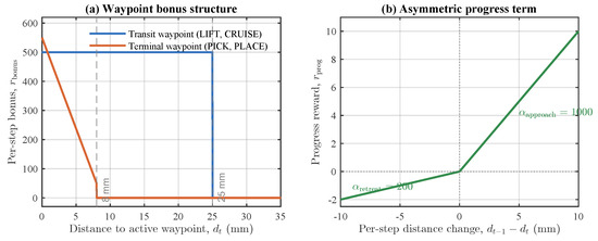
with $c_{\mathrm{step}}=0.02$. For the intermediate lift and cruise phases, a flat bonus of 500 is applied inside the 25 mm scheduler region. For the terminal pick and place phases, the adopted graded bonus is

$$r_{\mathrm{bonus}}=50+500\left(1-{\displaystyle \frac{d_t^{\mathrm{mm}}}{8}}\right),d_t^{\mathrm{mm}}<8\mathrm{mm}.$$

(33)

The terminal bonus, therefore, retains an interior distance gradient within the 8 mm region, whereas the intermediate-waypoint bonus remains constant after entry into the 25 mm region. Figure 5 summarises the adopted reward components.

Figure 5. Shaped reward components: (a) flat 500-point intermediate-waypoint bonus inside 25 mm and graded terminal-waypoint bonus inside 8 mm; and (b) asymmetric active-waypoint progress term. The 8 mm place region is used for reward shaping, while full-task success requires first entry within 5 mm.

The development-stage reward and scheduler configurations are compared in Section 6.5.

4.3. Simulink Environment and Experimental Protocol

The experimental protocol comprises episode initialisation, SAC training, nominal evaluation, post-entry continuation, frozen-policy robustness and generalisation tests, and conventional baseline comparisons. Unless stated otherwise, the experiments use the nominal waypoints, scheduler tolerances, plant model, controller parameters, timing, actuator constraints, and strict 5 mm terminal criterion specified above.

4.3.1. Environment Initialisation

Each nominal episode begins from a randomised joint configuration. For each joint,

$${\theta }_{j,0}\sim \mathcal{U}(-{20}^{\circ },{20}^{\circ }).$$

(34)

Rejection sampling requires the initial end-effector position to be more than 150 mm from the pick waypoint, with a maximum of 100 sampling attempts. The accepted joint values initialise the six Simulink joint-state integrators.

4.3.2. Training Protocol

The environment uses a fixed-step fourth-order Runge–Kutta solver with $T_{\mathrm{sim}}=0.005$ s, while the SAC agent operates at $T_{\mathrm{SAC}}=0.050$ s. Each 15 s episode, therefore, permits a maximum of 300 SAC decisions and 3000 simulation steps.

Training was configured for a maximum of 3000 episodes. The primary seed-0 run was manually stopped at episode 2719, and the corresponding policy was retained for the primary analyses. A second independently initialised run used seed 1 with the same environment, network architecture, reward function, SAC hyperparameters, and controller configuration. For a matched episode budget, the seed-1 policy was also retained at episode 2719.

These two training initialisations provide a limited sensitivity check and do not constitute a comprehensive assessment of SAC training reproducibility. Training statistics for the primary seed-0 run are reported in Section 6.1; the nominal seed-1 evaluation is reported in Section 6.2.

4.3.3. Main Evaluation Protocol

The retained seed-0 and seed-1 policies were each evaluated over 50 episodes using the same sequence of nominal randomised initial configurations. The seed-0 policy was retained as the primary policy for the detailed nominal, robustness, and post-entry evaluations. The seed-1 policy was used only for the independent nominal training-initialisation comparison.

The following metrics were recorded for each episode:

• Completion of each waypoint phase;
• Full-task success under the strict 5 mm place criterion;
• Minimum Cartesian distance to each active waypoint;
• Episode duration and accumulated reward;
• Joint-angle and joint-velocity limit compliance;
• Per-joint voltage-saturation activity.

For successful episodes, the distance recorded at the first crossing of the 5 mm criterion is treated as a threshold-entry measurement rather than steady-state placement accuracy. Post-entry behaviour was evaluated separately by continuing the 48 successful seed-0 runs for 2 s after strict place entry. Retention within 5 mm was assessed over 0.5, 1.0, and 2.0 s dwell intervals using the same 50 evaluation seeds.

4.3.4. Robustness and Generalisation Protocol

The retained seed-0 policy was evaluated without retraining under six modified conditions. Unless explicitly modified, the nominal LQR gains, timing, task logic, actuator constraints, and strict 5 mm criterion were retained. Each condition comprised 50 episodes.

• Broader initial configurations. The per-joint reset range was expanded from $\pm {20}^{\circ }$ to $\pm {30}^{\circ }$. Every accepted configuration contained at least one joint satisfying $|{\theta }_j|>{20}^{\circ }$ and retained the minimum 150 mm initial distance from the pick waypoint.
• Unseen shifted-waypoint configuration. The complete waypoint sequence was translated by ${[15,10,5]}^{\mathsf{T}}$ mm, giving

  $$\begin{array}{cccc}\hfill {\mathbf{p}}_{\mathrm{pick}}& ={[-365,-160,125]}^{\mathsf{T}},\hfill & \hfill {\mathbf{p}}_{\mathrm{lift}}& ={[-365,-160,185]}^{\mathsf{T}},\hfill \\ \hfill {\mathbf{p}}_{\mathrm{cruise}}& ={[-275,-100,270]}^{\mathsf{T}},\hfill & \hfill {\mathbf{p}}_{\mathrm{place}}& ={[-185,-40,305]}^{\mathsf{T}}\hfill \end{array}$$

  (35)

  in millimetres. The nominal scheduler tolerances and strict terminal criterion were unchanged.
• Model-parameter perturbations. The inertia $J_j$ and damping $b_j$ parameters were independently perturbed within $\pm 10\%$ of their nominal values at the beginning of each episode. The nominal LQR gains were retained.
• SAC observation-vector noise. Zero-mean Gaussian noise with ${\sigma }_{\mathrm{obs}}=0.01$ was added to the normalised 27-dimensional SAC observation before clipping to the nominal range.
• Command delay. A fixed 50 ms delay, corresponding to one SAC decision interval, was inserted in the joint-reference path before the six LQR loops.
• External torque disturbance. A $-0.5$ N·m torque was applied to joint 2 from 5.0 to 5.5 s.

Full-task success was evaluated using the nominal ordered phase logic and strict 5 mm place criterion. Success counts and Wilson 95% confidence intervals are reported in Section 6.4.

4.3.5. Conventional Baseline Protocols

Three conventional configurations were evaluated using the same nominal task-success criterion and paired initial-condition protocol.

The first two configurations used matched offline-reference LQR and PID tracking. A bank of 50 episode-specific joint-reference trajectories was generated before the final evaluation. For each paired initial configuration, position-only numerical inverse kinematics was solved sequentially for the pick, lift, cruise, and place waypoints. Rest-to-rest quintic joint-space trajectories connected the resulting joint configurations.

Each moving segment lasted 1.5 s and was followed by a 1.5 s dwell interval. The final place configuration was held until the 15 s episode horizon, and reference samples were supplied at 50 ms intervals. The complete trajectory bank was frozen and reused unchanged during the final comparison; no SAC inference, online inverse kinematics, or trajectory regeneration was performed.

For each paired episode, the matched LQR and PID configurations used the same reference trajectory, initial configuration, plant model, timing, limits, waypoint tolerances, and strict success criterion. They differed only in the local regulator. Table 8 lists the per-joint PID gains.

Table 8. Per-joint PID gains used in the matched offline-trajectory PID baseline.

Joint	${\mathit{K}}_{\mathit{p}}$	${\mathit{K}}_{\mathit{i}}$	${\mathit{K}}_{\mathit{d}}$
1	1256.4585	2078.5281	189.8805
2	1237.7504	2037.5252	187.9763
3	1178.1788	1921.4763	180.6040
4	1143.9687	1833.7111	178.4175
5	1132.7953	1805.0632	177.7258
6	1123.9768	1784.6513	176.9707

The third configuration was a separately implemented conventional IK–trajectory–LQR baseline. It did not use the SAC policy or the frozen matched-reference bank. Position-only numerical inverse kinematics determined the four-waypoint joint configurations, which were connected by rest-to-rest quintic trajectories and tracked using the implemented LQR inner-loop structure.

The conventional baseline used the same 1.5 s motion and 1.5 s dwell durations, with the terminal configuration held until 15 s. It also used the same plant, waypoints, scheduler tolerances, actuator constraints, strict success criterion, and nominal randomised initial-condition protocol as the Hybrid SAC–LQR evaluation.

The IK–trajectory–LQR baseline was additionally evaluated over 50 episodes under each of the five applicable modified conditions: the broader $\pm {30}^{\circ }$ initial range, shifted waypoints, $\pm 10\%$ model-parameter perturbations, the 50 ms reference delay, and the external joint-2 torque disturbance. Observation-vector noise was not applicable because this baseline does not use the SAC observation. The modified-condition comparison, therefore, comprised 250 conventional baseline episodes.

These protocols compare state-conditioned SAC reference generation with precomputed and conventional model-based reference-generation approaches under common task criteria; they do not presume a performance advantage for any configuration.

4.3.6. Implementation

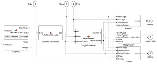
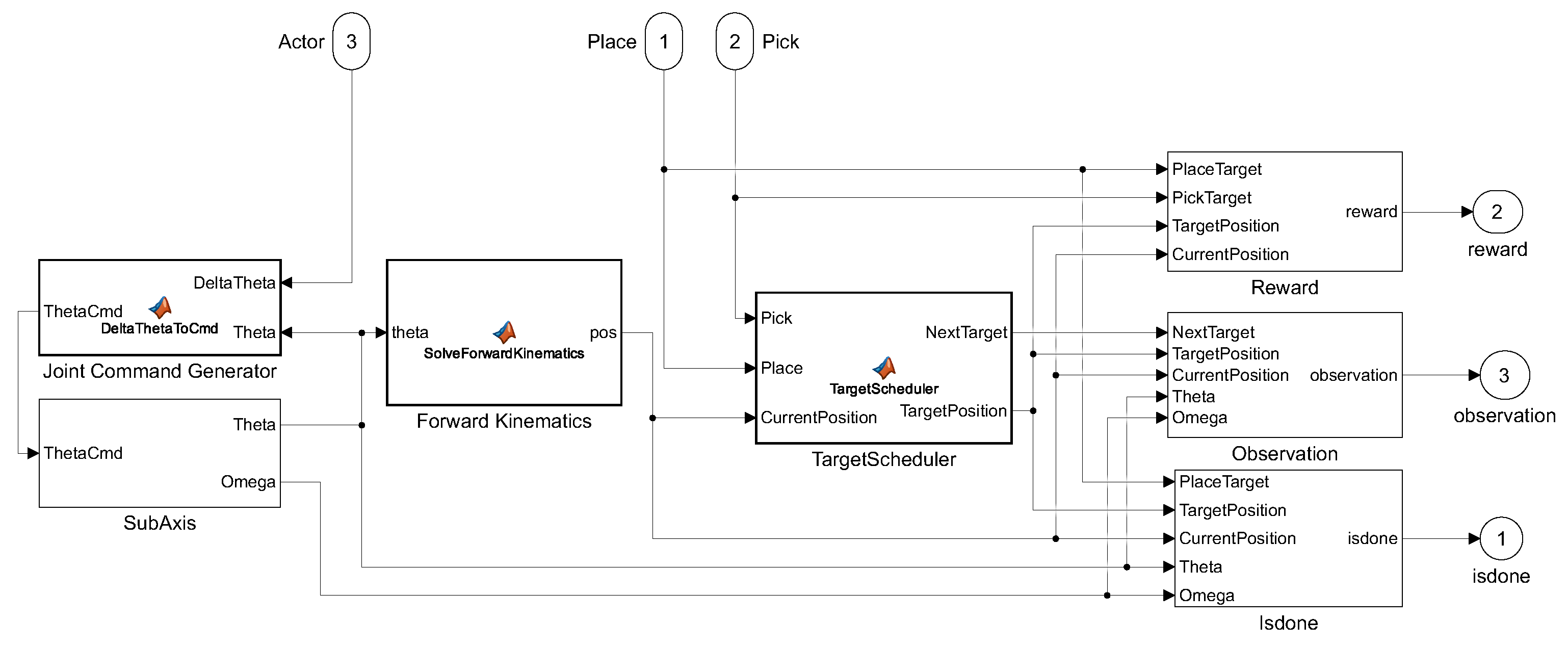
The complete Hybrid SAC–LQR framework was implemented using MATLAB R2024b, Simulink R2024b, and Reinforcement Learning Toolbox R2024b (The MathWorks, Inc., Natick, MA, USA). Figure 6 shows the top-level model, including the SAC agent, joint-reference conversion, six LQR loops, simplified joint plants, forward kinematics, phase scheduler, reward calculation, and termination logic.

Figure 6. Top-level Simulink implementation of the Hybrid SAC–LQR framework. The SAC agent operates at $T_{\mathrm{SAC}}=50$ ms, while the simplified plant and six LQR loops operate at $T_{\mathrm{sim}}=5$ ms.

Training and simulation were performed on a Windows 11 Pro 24H2 workstation equipped with an AMD Ryzen 7 5800H processor, 32 GB of random-access memory (RAM), and an NVIDIA GeForce RTX 3080 Laptop graphics processing unit (GPU).

5. MATLAB–ROS 2 Controller-Pipeline Evaluation

5.1. Evaluation Scope and Software Stack

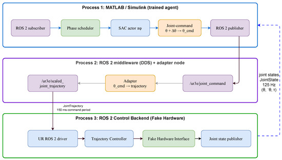
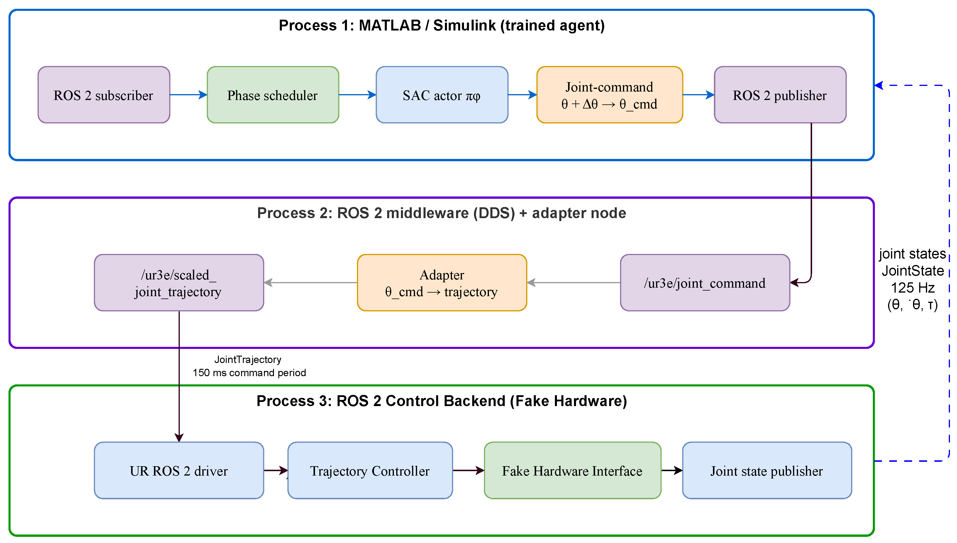
Following the MATLAB/Simulink evaluation, the trained SAC decision layer and task logic were assessed through an adapted MATLAB–ROS 2 controller pipeline. This stage evaluates controller-interface execution and communication separately from the complete Hybrid SAC–LQR architecture. Figure 7 shows the resulting pipeline and the exchange of joint commands and joint-state feedback between MATLAB/Simulink and ROS 2.

Figure 7. Adapted MATLAB–ROS 2 controller-pipeline architecture showing the SAC decision layer, waypoint scheduler, ROS 2 controller interface, and joint-state feedback path.

The adapted pipeline does not execute the Simulink per-joint plant or the six LQR inner loops described in Section 4. Instead, the SAC policy and waypoint scheduler generate joint commands in MATLAB/Simulink and exchange them with the ROS 2 controller interface through publisher and subscriber connections. Joint-state feedback is returned to the task logic for observation construction and phase progression.

The controller-pipeline software stack comprised ROS 2 Humble Hawksbill running on Ubuntu 22.04.5 LTS under Windows Subsystem for Linux 2 (WSL2), together with the Universal Robots ROS 2 driver, ros2_control, and the scaled_joint_trajectory_controller. The driver was configured with use_fake_hardware=true, allowing joint commands to propagate through the controller interface without a physical robot or the graphical URSim controller backend. This stage, therefore, characterises the SAC decision pipeline, middleware, and controller interface rather than the complete Hybrid SAC–LQR system.

5.2. Online Controller-Pipeline Execution

The trained SAC agent was loaded into the adapted model and executed using its mean action. The experiment retained the four nominal Cartesian waypoints and scheduler tolerances used in the main MATLAB/Simulink task.

At each update, the latest joint-state feedback is used to calculate the end-effector position. The scheduler supplies the active and next waypoints, after which the observation block constructs the 27-dimensional vector. The SAC actor generates $\Delta \mathit{\theta }$, which is combined with the measured joint configuration to form

$${\mathit{\theta }}_{\mathrm{cmd}}=\mathit{\theta }+\Delta \mathit{\theta }.$$

(36)

The resulting policy-generated command is then processed according to the terminal-assistance condition defined in Section 5.4. The final joint command is published through the ROS 2 interface and forwarded to the scaled_joint_trajectory_controller. Updated joint-state feedback is subsequently returned to MATLAB/Simulink for the next controller-pipeline update.

5.3. Communication Interface and Latency Measurement

The ROS 2 communication interface uses separate topics for joint commands and returned joint states. The command-side adapter converts the six-joint command generated by MATLAB/Simulink into a trajectory message accepted by the scaled joint-trajectory controller. MATLAB reads the returned joint-state information to reconstruct $\mathit{\theta }$ and estimate the corresponding joint-velocity vector.

The communication and controller settings are summarised in Table 9.

Table 9. Communication and controller settings for the adapted MATLAB–ROS 2 pipeline evaluation.

Setting	Configuration
ROS 2 distribution	Humble
Robot driver	Universal Robots ROS 2 driver
Controller framework	ros2_control
Backend	Fake hardware
Trajectory controller	scaled_joint_trajectory_controller
Command topic	/ur3e/joint_command
Feedback topic	/ur3e/joint_states
Command-publishing period	150 ms
ROS domain identifier	42
Middleware	Fast Data Distribution Service (Fast DDS)
Episode horizon	45 s

Communication latency was measured independently using a 60 s sinusoidal command probe sampled every 50 ms, yielding 1200 command–feedback observations. Round-trip latency was defined as the elapsed time between command transmission and receipt of the corresponding controller-side joint-state update. This experiment was conducted separately from the task-success evaluation to avoid combining communication timing with phase-dependent trajectory execution.

5.4. Controller-Pipeline Evaluation Protocol

The controller-pipeline evaluation used a protocol adapted to the ROS 2 controller interface. The initial joint configuration was fixed at

$${\mathbf{q}}_0={\left[\begin{array}{cccccc}0& 0& 0& 0& 0& 0\end{array}\right]}^{\mathsf{T}}.$$

(37)

The command-publishing period was 150 ms, and the maximum episode duration was 45 s. These settings were held constant throughout the controller-pipeline evaluation.

Two terminal-assistance conditions were evaluated. In the assist-enabled condition, the TerminalThetaAssist block supplied stored waypoint joint configurations near selected phase boundaries and throughout the final place phase. Specifically, ${\mathbf{q}}_{\mathrm{PICK}}$ replaced the policy-generated command when $\varphi =1$ and the pick distance was below 25 mm; ${\mathbf{q}}_{\mathrm{CRUISE}}$ was applied when $\varphi =3$ and the cruise distance was below 70 mm; and ${\mathbf{q}}_{\mathrm{PLACE}}$ was applied throughout $\varphi =4$. In the assist-disabled condition, the block was bypassed, and the policy-generated command passed through unchanged.

The stored joint configurations, expressed in radians, were

$$\begin{array}{cc}\hfill {\mathbf{q}}_{\mathrm{PICK}}& ={\left[\begin{array}{cccccc}-0.0973& 0.0859& -0.2641& 0.7387& -0.5966& -0.4357\end{array}\right]}^{\mathsf{T}},\hfill \\ \hfill {\mathbf{q}}_{\mathrm{CRUISE}}& ={\left[\begin{array}{cccccc}-0.1542& -0.1146& -0.6515& 1.1802& -1.2759& -0.5363\end{array}\right]}^{\mathsf{T}},\hfill \\ \hfill {\mathbf{q}}_{\mathrm{PLACE}}& ={\left[\begin{array}{cccccc}-0.3435& 0.0027& -1.3786& 1.6542& -1.7543& -0.4802\end{array}\right]}^{\mathsf{T}}.\hfill \end{array}$$

(38)

These configurations were extracted from a successful MATLAB/Simulink trajectory. Outside their respective activation conditions, the policy-generated command remained unchanged. The terminal-assistance logic is provided in Appendix A, Algorithm A2.

Using the same forward-kinematics model as the MATLAB/Simulink evaluation, the stored terminal configuration corresponds to

$$\mathrm{FK}\left({\mathbf{q}}_{\mathrm{PLACE}}\right)={[-202.614,-48.861,303.167]}^{\mathsf{T}}\mathrm{mm},$$

(39)

where $\mathrm{FK}(·)$ denotes the forward-kinematics mapping. This position is approximately 4.261 mm from the nominal place waypoint.

Each condition comprised 50 runs using the same trained SAC agent, fixed initial joint configuration, nominal waypoints, scheduler tolerances, ROS 2 configuration, command-publishing period, and episode horizon. The phase-completion and full-task success results are reported in Section 6.7.

Although the initial configuration and policy were fixed, the repeated controller-pipeline runs were not bitwise time-synchronised. Small run-to-run differences may, therefore, arise from controller initialisation, asynchronous command–feedback timing, ROS 2 middleware scheduling, and phase-transition timing. These effects can produce slightly different sampled state-transition sequences under otherwise identical settings.

5.5. Excluded URSim Controller-Backend Stage

An additional controller-backend stage was attempted through URSim with use_fake_hardware=false and the External Control interface. Initial tests confirmed ROS 2 driver connectivity and access to the URSim dashboard. However, reliable execution through the graphical PolyScope/URSim backend could not be completed in the available Windows Subsystem for Linux 2 (WSL2)/Docker environment because the PolyScope/noVNC interface became unresponsive after restarting the External Control plugin.

This controller-backend experiment was, therefore, excluded from the reported quantitative evaluation.

6. Results

This section reports the evaluation of the Hybrid SAC–LQR framework and the associated comparison experiments. The complete architecture is first evaluated in MATLAB/Simulink under randomised initial joint configurations. Additional experiments examine representative closed-loop behaviour, robustness and generalisation, reward-design variations, post-entry placement behaviour, the adapted MATLAB–ROS 2 controller pipeline, and conventional baselines. Unless otherwise stated, each condition comprises 50 episodes.

6.1. Training Behaviour

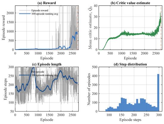
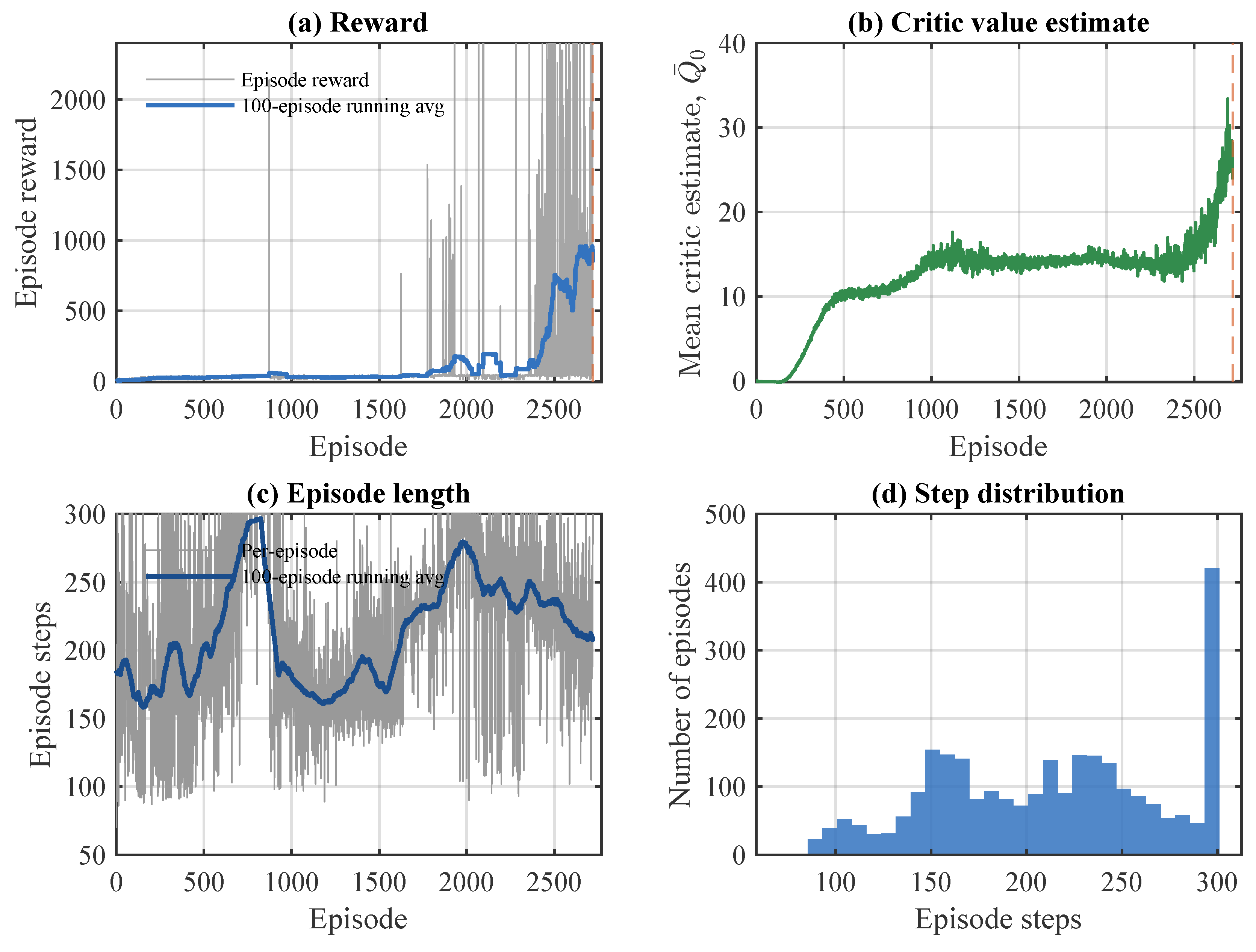
The primary seed-0 SAC agent was trained using the four-phase pick–lift–cruise–place curriculum described in Section 4. The retained policy corresponds to episode 2719 of the manually stopped training run. Figure 8 shows the recorded training behaviour up to the retained policy.

Figure 8. Training behaviour of the primary seed-0 SAC agent: (a) episode reward and 100-episode running-average reward; (b) critic initial-state value estimate; (c) episode length and 100-episode running-average episode length; and (d) episode-length distribution. The orange dashed vertical line in panels (a,b) marks the retained policy checkpoint at episode 2719.

At the retained checkpoint, the 100-episode running-average reward was 933.97, the maximum recorded running-average reward was 960.00, and the critic initial-state value estimate was $Q_0=23.86$. These quantities describe the recorded training state and are not interpreted as evidence of convergence or a performance plateau. The retained policy was subsequently used without further training for the main evaluation and frozen-policy robustness tests.

6.2. Main Randomised Hybrid SAC–LQR Evaluation

The complete Hybrid SAC–LQR architecture was evaluated over 50 episodes using randomised initial joint configurations generated by the nominal reset protocol. Forty-eight episodes completed the ordered four-phase task and entered the strict 5 mm place-success region, corresponding to 48/50 successes (96%; Wilson 95% confidence interval (CI): 86.54–98.90%).

The same 48 episodes satisfied all preceding phase transitions. The two unsuccessful episodes did not advance beyond the initial pick phase. The aggregate evaluation metrics are summarised in Table 10.

Table 10. Main MATLAB/Simulink evaluation results for the complete Hybrid SAC–LQR configuration over 50 randomised episodes.

Metric	Result
Evaluation episodes	50
Full-task successes	48/50
Full-task success rate	96%
Wilson 95% CI	86.54–98.90%
Mean episode reward	4366.3
Mean episode duration	9.72 s
Successful place termination distance	$4.221\pm 0.381$ mm
Median successful place termination distance	4.256 mm
Joint-limit violations	0
Voltage-saturation duty cycle	0.0% for all joints

Table 11 distinguishes the minimum active-phase distances retained by the scheduler from the strict successful place termination values. Because unsuccessful episodes may remain far from later waypoints, the all-episode place distribution is substantially wider than the successful-episode distribution.

Table 11. Minimum Cartesian distance to each active waypoint during the 50-episode nominal evaluation. The final row reports the 48 successful episodes at strict place termination.

Phase/metric	Mean (mm)	Median (mm)	Std. Dev. (mm)
pick	8.100	8.047	0.126
lift	25.997	25.225	4.088
cruise	30.631	25.037	27.714
place, all episodes	14.723	4.284	51.984
place, successful episodes	4.221	4.256	0.381

The reported $4.221\pm 0.381$ mm value is the Cartesian distance at first entry into the strict 5 mm place region and is, therefore, a threshold-entry metric rather than steady-state positioning accuracy. For context, a separately trained seed-1 policy achieved 45/50 nominal full-task successes (90%) under the same evaluation protocol. This limited training-initialisation check was not used for the detailed analyses or modified-condition tests reported below, which use the retained seed-0 policy.

6.3. Representative Closed-Loop Behaviour

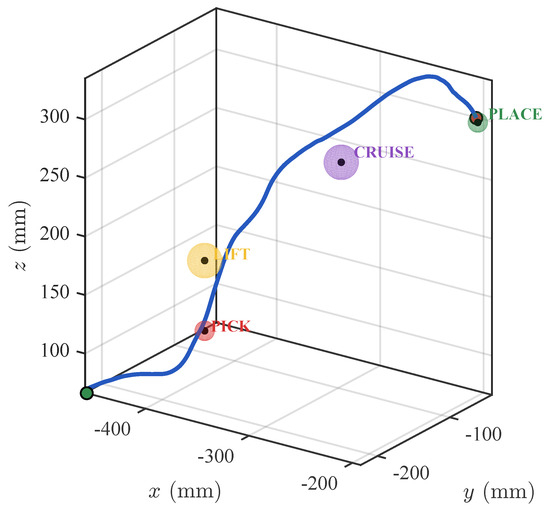
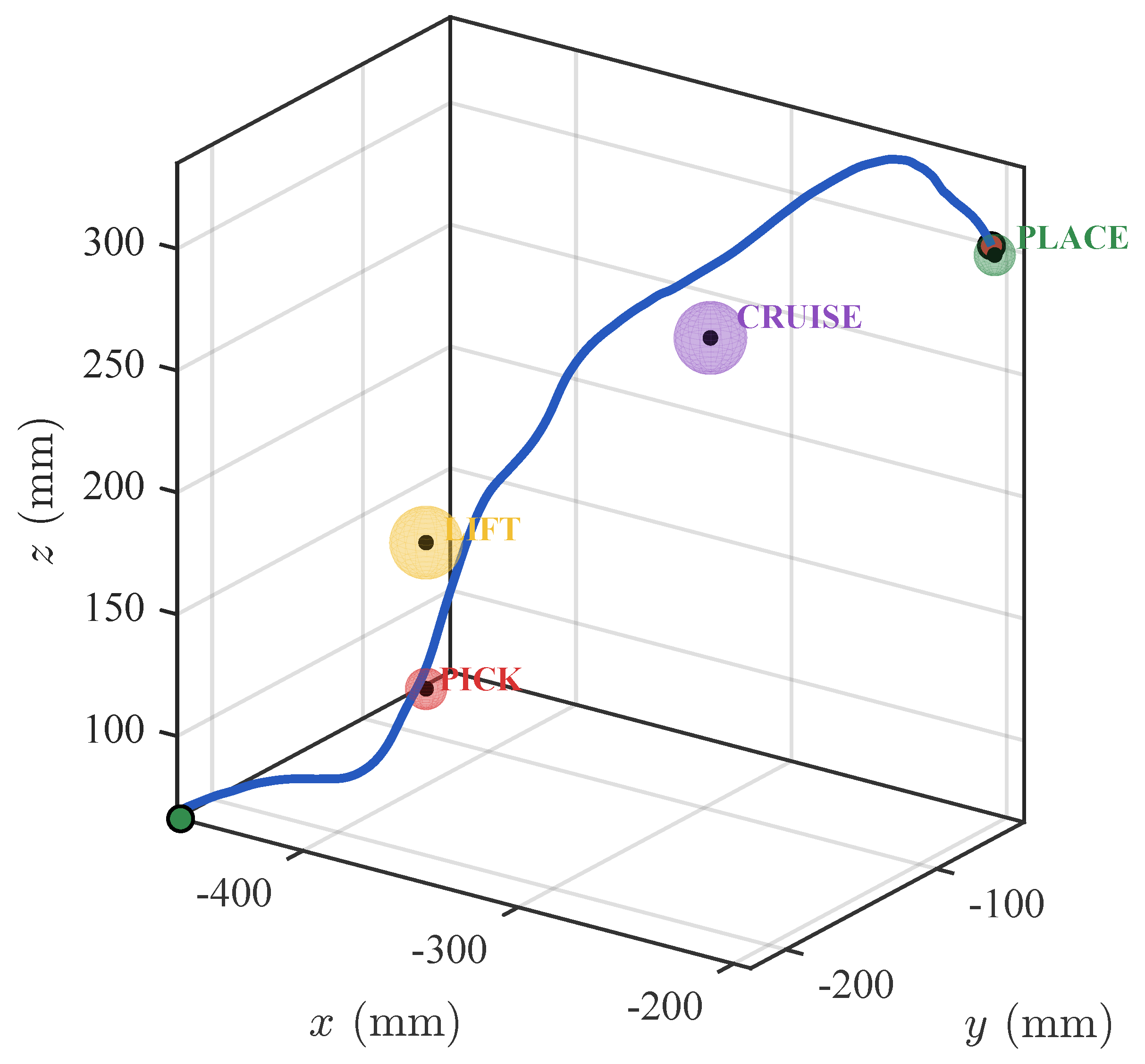
A representative successful MATLAB/Simulink episode shows the end effector progressing through the four-waypoint sequence into the strict place-success region. Figure 9 shows the corresponding three-dimensional end-effector path.

Figure 9. Representative three-dimensional end-effector trajectory through the four-waypoint sequence.

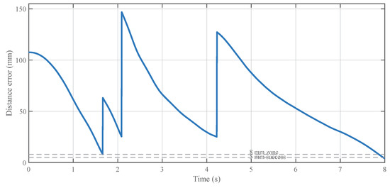
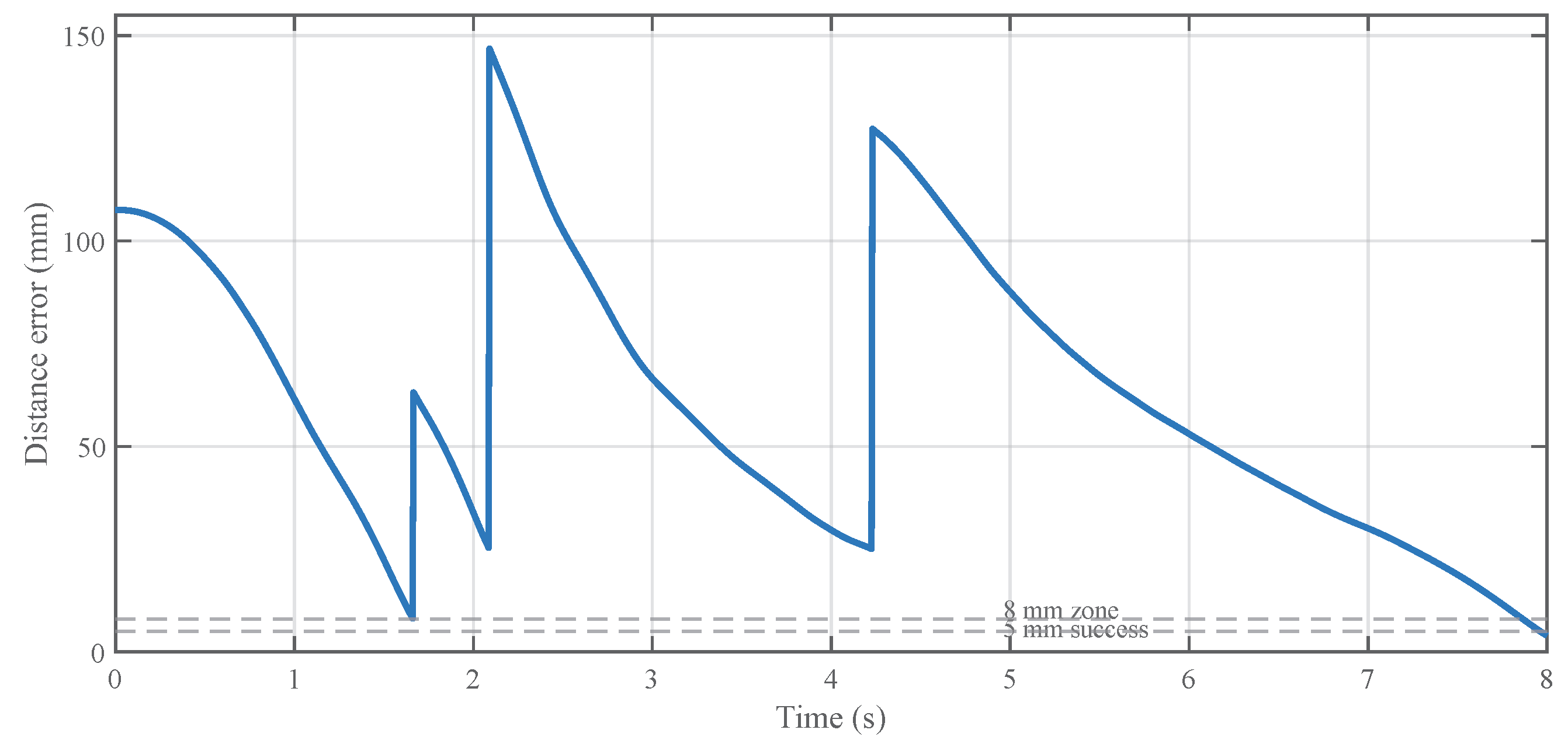
Figure 10 shows the active-waypoint distance during the same episode. The apparent discontinuities result from scheduler target changes, while the end-effector trajectory remains continuous across phase transitions.

Figure 10. Active-waypoint distance during the representative successful episode.

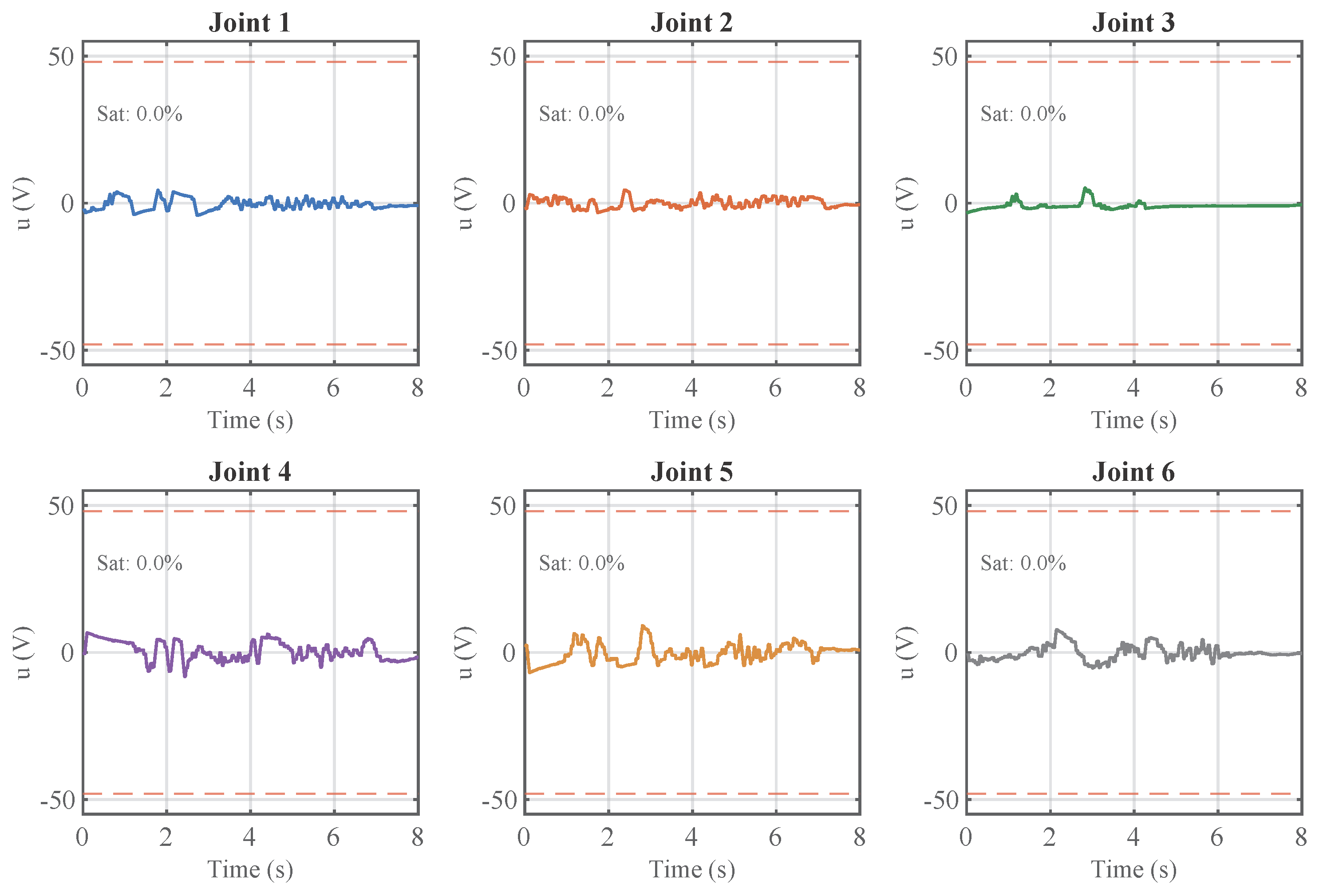
The corresponding joint-angle, joint-velocity, and per-axis motor-voltage trajectories are provided in Appendix A, Figure A1 and Figure A2. Joint angles remained within the $\pm 2\pi$ rad software limits, while joint velocities remained within the adopted limits of $\pm \pi$ rad/s for joints 1–3 and $\pm 2\pi$ rad/s for joints 4–6.

Across all 50 nominal MATLAB/Simulink evaluation episodes, the voltage-saturation duty cycle was 0.0% for every joint, with no sampled saturation events under the adopted $\pm 48$ V limit.

6.4. Robustness and Generalisation

The retained SAC policy was evaluated without retraining under six modified conditions. The conventional IK–trajectory–LQR baseline was also evaluated under the five applicable modified conditions using 50 episodes per condition. Table 12 reports the full-task success results and Wilson 95% confidence intervals.

Table 12. Robustness and generalisation results for the retained Hybrid SAC–LQR policy and the conventional IK–trajectory–LQR baseline. Each applicable condition contains 50 evaluation episodes.

Condition	Hybrid Success	Hybrid Wilson 95% CI	IK–LQR Success	IK–LQR Wilson 95% CI
Nominal evaluation	48/50 (96%)	86.54–98.90%	50/50 (100%)	92.87–100%
Broader initial range ($\pm {30}^{\circ }$)	48/50 (96%)	86.54–98.90%	43/50 (86%)	73.81–93.05%
Unseen shifted-waypoint configuration	50/50 (100%)	92.87–100%	50/50 (100%)	92.87–100%
Simultaneous model-parameter perturbations ($\pm 10\%$)	48/50 (96%)	86.54–98.90%	50/50 (100%)	92.87–100%
SAC observation-vector noise (${\sigma }_{\mathrm{obs}}=0.01$)	41/50 (82%)	69.20–90.23%	Not applicable	Not applicable
Command delay (50 ms)	43/50 (86%)	73.81–93.05%	50/50 (100%)	92.87–100%
External torque, joint 2 ($-0.5$ N·m, 5.0–5.5 s)	47/50 (94%)	83.78–97.94%	50/50 (100%)	92.87–100%

The retained policy preserved the nominal 96% success rate under the broader initial range and the tested model-parameter perturbation. The shifted-waypoint configuration was completed in all 50 episodes. The strongest performance reductions occurred under observation noise and command delay, where success decreased to 82% and 86%, respectively. The external joint-2 torque disturbance produced a smaller reduction, with success decreasing to 94%. The successful observation-noise episodes terminated at $4.665\pm 0.200$ mm, whereas the successful external-disturbance episodes terminated at $4.232\pm 0.400$ mm.

The IK–trajectory–LQR baseline completed all nominal, shifted-waypoint, model-perturbation, command-delay, and external-torque episodes. Under the broader initial range, it completed 43/50 episodes. In the seven unsuccessful episodes, the fixed-time trajectory did not enter the pick tolerance within the allocated phase interval; these cases were not caused by inverse-kinematics infeasibility or closed-loop instability. Observation noise was not applicable to this baseline because it does not use the 27-dimensional SAC observation vector.

6.5. Reward-Design Comparison

Several development-stage reward and scheduler configurations were evaluated to examine their effect on strict full-task completion. The tested configurations included both structural reward changes and numerical variations in waypoint-transition settings.

A flat terminal bonus inside the 8 mm region did not produce strict full-task completion. A graded terminal formulation with an 80 mm approach region, likewise, resulted in 0% strict full-task success, as did widening the intermediate transit tolerance from 25 to 40 mm. The adopted configuration retained the original 25 mm intermediate tolerances and applied graded terminal shaping inside the 8 mm terminal region, achieving the reported 96% full-task success rate.

These results summarise the development-stage reward-design comparisons used in selecting the final configuration.

6.6. Post-Entry Placement Behaviour

The nominal evaluation terminates when the end effector first enters the strict 5 mm place region. To characterise the subsequent positioning behaviour, a separate modified continuation evaluation used the same 50 evaluation seeds. Of these runs, 48 achieved strict place entry and provided valid 2 s post-entry observation windows.

None of the 48 runs remained continuously below 5 mm over the complete 0.5, 1.0, or 2.0 s intervals. Over the 2 s continuation, the mean retention within the 5 mm region was $14.82\pm 0.35\%$. The mean Cartesian position error over the final 0.5 s was $8.606\pm 0.093$ mm, with a mean maximum post-entry error of $9.002\pm 0.143$ mm. Thus, settling within the 5 mm region was not observed.

The mean post-entry Cartesian path length was $21.551\pm 0.853$ mm, and the mean control effort was $6.095\pm 0.152$ V²s. Because no end-effector orientation target was specified for the position-only task, the angular measure is reported as orientation drift from first strict place entry rather than as orientation error relative to a prescribed pose. Its mean value across the 48 runs over the 2 s interval was $54.693\pm 0.{568}^{\circ }$.

The narrow variation in the final-window position error is consistent with a repeatable post-entry offset; this observation does not, by itself, establish closed-loop stability. This behaviour is consistent with the implemented inner-loop structure described in Section 4.1.3: the design-only integral state is not accumulated during execution, and the implemented controller, therefore, has finite steady-state tracking gain. Under a held joint reference, this can produce a non-zero joint-level static tracking offset that propagates through the forward kinematics. The observed post-entry offset is, therefore, associated with the combined reference command and implemented inner-loop regulation rather than with the SAC policy alone.

The nominal $4.221\pm 0.381$ mm value, therefore, characterises the position error at first entry into the strict place region, whereas the continuation results characterise the subsequent post-entry positioning behaviour.

6.7. Adapted MATLAB–ROS 2 Controller-Pipeline Evaluation

The adapted controller-pipeline experiment described in Section 5 was evaluated separately from the complete Hybrid SAC–LQR simulation. This stage used deterministic SAC action selection, a fixed zero initial joint configuration, a 150 ms command-publishing period, a 45 s episode horizon, the ros2_control fake-hardware backend, and no Simulink per-joint plant or LQR inner loops.

Two 50-run conditions were evaluated: terminal assistance enabled and terminal assistance disabled. Both conditions used the same trained policy, initial configuration, controller interface, command-publishing period, episode horizon, waypoint sequence, and task criteria. The results are reported in Table 13.

Table 13. Terminal-assistance comparison in the adapted MATLAB–ROS 2 controller pipeline.

Metric	Assist Enabled	Assist Disabled
pick success	98% (49/50)	66% (33/50)
lift success	98% (49/50)	64% (32/50)
cruise success	96% (48/50)	32% (16/50)
place$< 8$ mm	96% (48/50)	0% (0/50)
Full task, strict 5 mm	96% (48/50)	0% (0/50)

With assistance disabled, the policy-generated commands supported progression through the intermediate phases in some runs, but none of the 50 runs reached the final place criterion. With assistance enabled, stored waypoint configurations were introduced near selected phase boundaries and throughout the final place phase, yielding 48 full-task completions. The difference between the two conditions, therefore, characterises the contribution of terminal assistance within the adapted controller pipeline.

For the assist-enabled condition, the mean successful place distance was $4.82\pm 0.04$ mm, close to the 4.261 mm forward-kinematics distance of the stored terminal configuration. The result is, therefore, consistent with execution of that configuration and characterises the terminal-assisted protocol rather than unassisted SAC reference generation. It does not characterise the LQR layer, which was not executed in this experiment.

The measured ROS 2 round-trip latency characterises the fake-hardware communication path. Its mean value was 5.45 ms, below the 50 ms SAC decision interval used in the complete MATLAB/Simulink architecture, whereas the adapted controller-pipeline experiment used a 150 ms command-publishing period. The latency statistics are summarised in Table 14.

Table 14. ROS 2 round-trip latency statistics from 1200 command–feedback observations.

Latency Statistic	Value (ms)
Mean	5.45
Median	5.65
Standard deviation	1.40
95th percentile	6.01
99th percentile	6.48
Maximum	25.10

These measurements should not be interpreted as physical-robot communication or closed-loop control timing.

6.8. Conventional Baseline Comparison

The Hybrid SAC–LQR framework was compared with three conventional controller configurations under the nominal protocols described in Section 4.3. The matched offline-trajectory LQR and PID configurations tracked the same episode-specific joint-reference bank under paired initial conditions, while the conventional IK–trajectory–LQR configuration generated its references independently using position-only inverse kinematics and quintic joint-space trajectories.

All configurations were evaluated over 50 episodes using the same waypoints, phase-transition tolerances, strict 5 mm success criterion, plant model, joint and voltage limits, and nominal initial conditions. Table 15 summarises the full-task success rates and successful place termination distances, reported as mean ± standard deviation.

Table 15. Nominal comparison of the Hybrid SAC–LQR framework and conventional controllers.

Method	Full-Task Success	Termination Distance (mm)
Hybrid SAC–LQR	96% (48/50)	$4.221\pm 0.381$
Matched offline-trajectory LQR	100% (50/50)	$4.888\pm 0.039$
Matched offline-trajectory PID	100% (50/50)	$4.561\pm 0.092$
Conventional IK–trajectory–LQR	100% (50/50)	$4.887\pm 0.031$

The three conventional configurations completed all 50 nominal episodes, compared with 48/50 for the Hybrid SAC–LQR framework. The termination distances represent first entry into the strict 5 mm place region rather than steady-state positioning error.

7. Discussion

7.1. Interpretation of the Main Findings

The complete Hybrid SAC–LQR framework completed the ordered four-phase task under most of the evaluated nominal initial configurations. The reported nominal place result represents first entry into the strict success region rather than sustained terminal positioning. The continuation evaluation did not show sustained sub-5 mm positioning. As explained in Section 6.6, the post-entry behaviour is consistent with the finite steady-state tracking gain of the implemented inner loop and reflects the combined reference command and local regulation rather than the SAC policy alone.

The frozen-policy evaluations characterised performance under the specified initial-state, waypoint, model-parameter, observation, command-delay, and external-disturbance conditions. Performance remained at or close to the nominal level under the broader initial range, shifted waypoints, model-parameter perturbation, and external torque, whereas the largest reductions occurred under observation noise and command delay. These results characterise the tested conditions and do not establish robustness beyond them.

The conventional comparisons provide context for the role of the learned decision layer. The three conventional configurations completed 50/50 nominal episodes, compared with 48/50 for the Hybrid SAC–LQR framework. The IK–trajectory–LQR baseline achieved 86–100% episode success under the five applicable modified conditions. These results confirm the effectiveness of conventional trajectory-based control for the considered waypoint task and do not establish a general performance advantage for learned reference generation. The Wilson confidence intervals quantify uncertainty in the individual success proportions; no claim of statistically significant superiority between the approaches is made.

Within the proposed architecture, the SAC layer is interpreted specifically as a mechanism for generating state-conditioned incremental joint references at runtime under varying initial configurations and sequential waypoint progression. It does not generate actuator torque or voltage commands. A direct comparison with pure SAC actuator-level control would require a different action space, environment, and independently trained policy rather than removal of the LQR layer from the present architecture.

The reward-development comparisons showed that strict task completion varied with the tested reward and scheduler configurations. The adopted graded terminal shaping and intermediate scheduler tolerances supported the reported nominal performance, whereas the three alternative configurations did not produce strict full-task completion. These comparisons document the evaluated development configurations rather than an exhaustive reward-hyperparameter optimisation.

The MATLAB–ROS 2 controller-pipeline evaluation addressed controller-interface execution and communication separately from the complete MATLAB/Simulink architecture. Full-task completion in this pipeline depended on the stored terminal-assistance configurations, whereas the assist-disabled condition did not complete the final place phase. The controller-pipeline results, therefore, characterise terminal-assisted pipeline execution rather than unassisted transfer of the retained policy. The latency measurements characterise the fake-hardware communication path and do not establish closed-loop physical-robot performance.

7.2. Limitations

The strict 5 mm success criterion measures first entry into the place region rather than sustained terminal positioning. The post-entry evaluation did not show that this accuracy was maintained, and the implemented inner-loop realisation does not provide offset-free tracking under a held reference. The first-entry distance should, therefore, remain distinct from steady-state placement accuracy.

The MATLAB/Simulink plant comprises simplified independent per-joint electromechanical models. It excludes coupled rigid-body dynamics, gravity, Coriolis and centrifugal effects, nonlinear friction, payload dynamics, and contact forces. The model-parameter perturbations and external torque disturbance extend the evaluation within this simplified setting but do not reproduce the coupled dynamics or payload-dependent behaviour of the physical manipulator. Likewise, the negative-real-part poles reported in Table 7 apply only to the isolated nominal unsaturated linear joint models. They do not provide a stability proof for the learned, multi-rate, nonlinear, and saturated closed-loop system.

The robustness and generalisation assessment is limited to the specified variations and their tested magnitudes. It does not establish performance under untested payload, contact, coupled-dynamics, or physical-robot conditions. The simulated task also represents position-based waypoint progression rather than a complete pick-and-place operation. Gripper dynamics, grasping, object transfer, release, end-effector orientation requirements, human–robot interaction, shared-workspace operation, and collaboration-specific safety logic were not modelled.

Training-initialisation sensitivity was assessed using the retained seed-0 policy and one independently initialised seed-1 policy. The second policy achieved 45/50 full-task successes under the nominal protocol, but two training initialisations are insufficient to characterise the distribution of training outcomes or establish training reproducibility.

The MATLAB–ROS 2 evaluation used the ros2_control fake-hardware backend, a fixed initial configuration, deterministic SAC action selection, a 150 ms command-publishing period, and a 45 s episode horizon. It did not execute the Simulink plant or the LQR inner loops, and successful full-task execution depended on terminal assistance. The results, therefore, represent controller-interface and communication-level testing rather than validation of the complete Hybrid SAC–LQR architecture, graphical URSim-controller execution, or physical UR3e operation.

7.3. Future Research Directions

Future evaluation should incorporate a coupled rigid-body UR3e model including gravity, Coriolis and centrifugal effects, nonlinear friction, payload variation, and contact forces. This would extend the evaluation beyond the independent per-joint models used in the present study.

The task model should subsequently include the gripper, object grasping, payload transfer, contact, and release. These additions would extend the current waypoint-progression task towards complete physical pick-and-place manipulation.

The controller-pipeline evaluation should be continued through a stable graphical URSim controller backend with use_fake_hardware=false and the External Control interface. Following controller-backend execution, the evaluation should proceed to experiments on a physical UR3e under appropriate operational and safety constraints.

A broader training assessment should include additional independent SAC initialisations evaluated under common nominal and modified conditions. This would provide a more complete characterisation of training variability beyond the two training runs considered in the present study.

8. Conclusions

This study presented a Hybrid SAC–LQR framework for a four-phase UR3e waypoint-control task. The SAC layer generated bounded, state-conditioned incremental joint references, while six per-joint LQR loops provided local reference tracking in MATLAB/Simulink. The retained policy completed 48/50 (96%) randomised nominal episodes. The successful place distance of $4.221\pm 0.381$ mm represents first entry into the strict 5 mm region; the separate continuation evaluation showed that this accuracy was not sustained over the evaluated post-entry dwell intervals.

Performance varied across the tested modified conditions, while the conventional trajectory-based baselines achieved 50/50 (100%) nominal completion. These comparisons do not establish a general performance advantage for the learned method. Instead, they position the SAC layer as a runtime mechanism for state-conditioned joint-reference generation within the evaluated architecture.

The separate MATLAB–ROS 2 fake-hardware experiment assessed controller-interface and communication-level execution. It did not validate the complete Hybrid SAC–LQR architecture or physical UR3e operation. Subject to the modelling, task, training, and deployment limitations identified above, the study provides a simulation-based evaluation of learned incremental reference generation combined with LQR-based local regulation.   

Appendix A.1. Scheduling Algorithms

Algorithm A1 summarises the phase-scheduling procedure described in Section 4.1.5.

Algorithm A1 Phase scheduler at each agent step.

Require: End-effector position $\mathbf{p}$, current phase $\varphi \in \{1,2,3,4\}$, waypoints $\{{\mathbf{g}}_1,{\mathbf{g}}_2,{\mathbf{g}}_3,{\mathbf{g}}_4\}$, and tolerances $\{{\tau }_1,{\tau }_2,{\tau }_3,{\tau }_4\}$.

Ensure: Active target ${\mathbf{g}}_{\mathrm{active}}$, next target ${\mathbf{g}}_{\mathrm{next}}$, and updated phase $\varphi$.

1: while $\varphi <4$ and $\parallel \mathbf{p}-{\mathbf{g}}_{\varphi }\parallel <{\tau }_{\varphi }$ do  2:     $\varphi \leftarrow \varphi +1$  3: end while  4: ${\mathbf{g}}_{\mathrm{active}}\leftarrow {\mathbf{g}}_{\varphi }$  5: ${\mathbf{g}}_{\mathrm{next}}\leftarrow {\mathbf{g}}_{\min (\varphi +1,4)}$  6: return ${\mathbf{g}}_{\mathrm{active}},{\mathbf{g}}_{\mathrm{next}},\varphi$

Algorithm A2 summarises the terminal-assistance logic used in the assist-enabled MATLAB–ROS 2 controller-pipeline condition described in Section 5.4.

Algorithm A2 Terminal-assist scheduling in the assist-enabled condition.

Require: Policy-generated command ${\mathit{\theta }}_{\mathrm{cmd}}$, phase $\varphi$, and current Cartesian position $\mathbf{p}$.

1: Compute $d_{\mathrm{PICK}}={\parallel \mathbf{p}-{\mathbf{p}}_{\mathrm{PICK}}\parallel }_2$.   2: Compute $d_{\mathrm{CRUISE}}={\parallel \mathbf{p}-{\mathbf{p}}_{\mathrm{CRUISE}}\parallel }_2$.   3: if $\varphi =1$ and $d_{\mathrm{PICK}}<25$ mm then   4:     ${\mathit{\theta }}_{\mathrm{cmd}}\leftarrow {\mathbf{q}}_{\mathrm{PICK}}$   5: else if $\varphi =3$ and $d_{\mathrm{CRUISE}}<70$ mm then   6:     ${\mathit{\theta }}_{\mathrm{cmd}}\leftarrow {\mathbf{q}}_{\mathrm{CRUISE}}$   7: else if $\varphi =4$ then   8:     ${\mathit{\theta }}_{\mathrm{cmd}}\leftarrow {\mathbf{q}}_{\mathrm{PLACE}}$   9: end if 10: return ${\mathit{\theta }}_{\mathrm{cmd}}$

Appendix A.2. Supporting Joint-Level Trajectories

Figure A1 and Figure A2 show the joint-level kinematic and motor-voltage trajectories for the representative successful episode discussed in Section 6.3.

Figure A1. Joint-angle and joint-velocity trajectories during the representative successful episode.

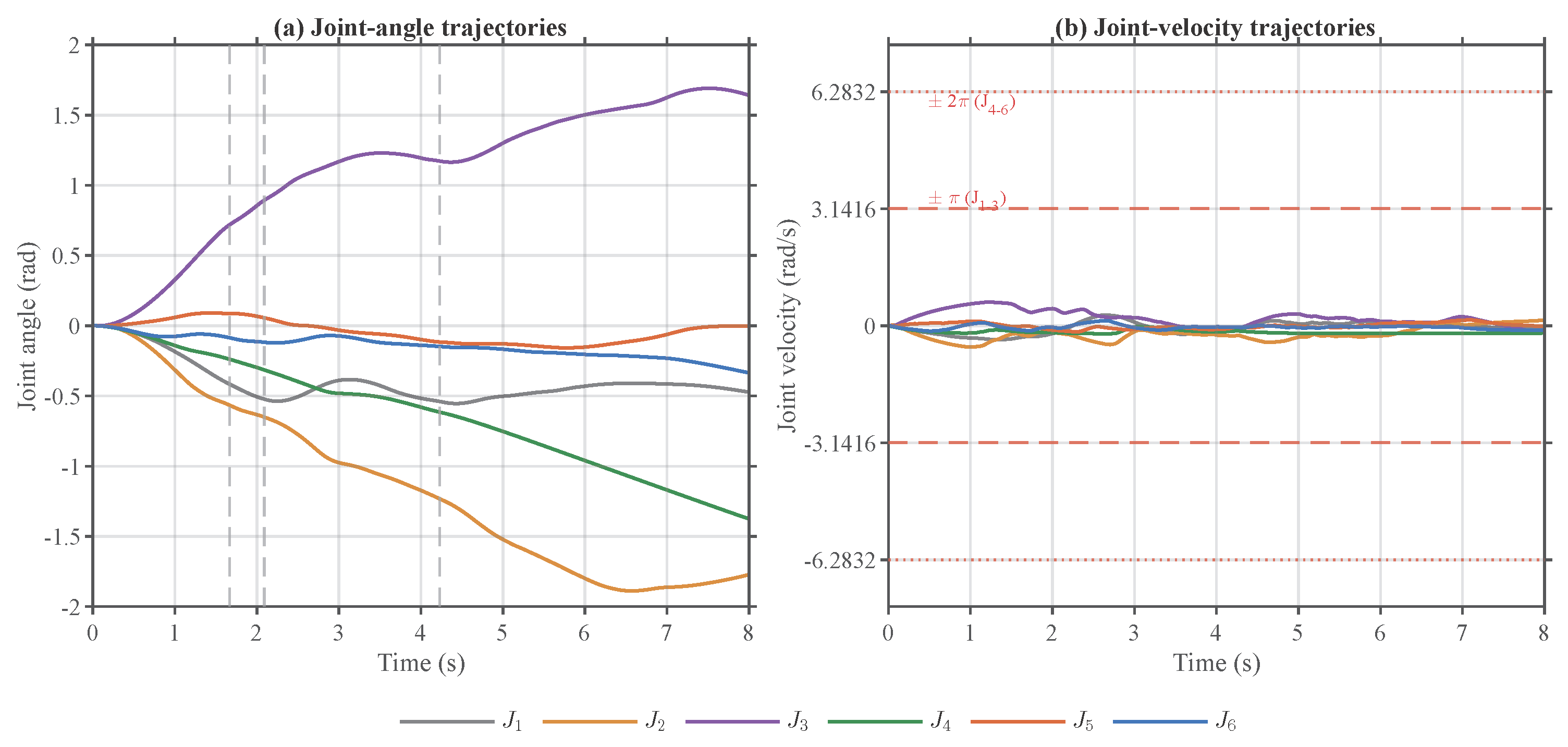
Figure A1. Joint-angle and joint-velocity trajectories during the representative successful episode.

Figure A2. Per-axis motor-voltage trajectories during the representative successful episode.

Figure A2. Per-axis motor-voltage trajectories during the representative successful episode.

References

- Gao, R.X.; Krüger, J.; Merklein, M.; Möhring, H.-C.; Váncza, J. Artificial intelligence in manufacturing: State of the art, perspectives, and future directions. CIRP Ann. 2024, 73, 723–749. [Google Scholar] [CrossRef] [Scilit]
- Kober, J.; Bagnell, J.A.; Peters, J. Reinforcement learning in robotics: A survey. Int. J. Robot. Res. 2013, 32, 1238–1274. [Google Scholar] [CrossRef] [Scilit]
- Han, D.; Mulyana, B.; Stankovic, V.; Cheng, S. A survey on deep reinforcement learning algorithms for robotic manipulation. Sensors 2023, 23, 3762. [Google Scholar] [CrossRef] [Scilit] [PubMed]
- Tang, C.; Abbatematteo, B.; Hu, J.; Chandra, R.; Martín-Martín, R.; Stone, P. Deep reinforcement learning for robotics: A survey of real-world successes. Annu. Rev. Control Robot. Auton. Syst. 2025, 8, 153–188. [Google Scholar] [CrossRef] [Scilit]
- Spong, M.W.; Hutchinson, S.; Vidyasagar, M. Robot Modeling and Control; John Wiley & Sons: Hoboken, NJ, USA, 2006. [Google Scholar]
- Siciliano, B.; Sciavicco, L.; Villani, L.; Oriolo, G. Robotics: Modelling, Planning and Control; Springer: London, UK, 2009. [Google Scholar] [CrossRef] [Scilit]
- Haarnoja, T.; Zhou, A.; Abbeel, P.; Levine, S. Soft actor-critic: Off-policy maximum entropy deep reinforcement learning with a stochastic actor. In Proceedings of the 35th International Conference on Machine Learning (ICML), Stockholm, Sweden, 10–15 July 2018; Proceedings of Machine Learning Research; International Conference on Machine Learning (ICML): San Diego, CA, USA, 2018; Volume 80, pp. 1861–1870. [Google Scholar]
- Shah, R.; Arockia Doss, A.S.; Lakshmaiya, N. Advancements in AI-enhanced collaborative robotics: Towards safer, smarter, and human-centric industrial automation. Results Eng. 2025, 27, 105704. [Google Scholar] [CrossRef] [Scilit]
- Gomes, N.M.; Martins, F.N.; Lima, J.; Wörtche, H. Reinforcement learning for collaborative robots pick-and-place applications: A case study. Automation 2022, 3, 223–241. [Google Scholar] [CrossRef] [Scilit]
- Kuo, P.-H.; Huang, C.-T.; Chang, C.-W.; Feng, P.-H.; Lin, Y.-S. Design and implementation of a soft actor–critic controller for a robotic arm. Eng. Appl. Artif. Intell. 2025, 151, 110589. [Google Scholar] [CrossRef] [Scilit]
- Lobbezoo, A.; Kwon, H.-J. Simulated and real robotic reach, grasp, and pick-and-place using combined reinforcement learning and traditional controls. Robotics 2023, 12, 12. [Google Scholar] [CrossRef] [Scilit]
- Elguea-Aguinaco, Í.; Serrano-Muñoz, A.; Chrysostomou, D.; Inziarte-Hidalgo, I.; Bøgh, S.; Arana-Arexolaleiba, N. A review on reinforcement learning for contact-rich robotic manipulation tasks. Robot. Comput.-Integr. Manuf. 2023, 81, 102517. [Google Scholar] [CrossRef] [Scilit]
- Fareh, R.; Siddique, T.; Choutri, K.; Dylov, D.V. Physics-informed reward-shaped reinforcement learning control of a robot manipulator. Ain Shams Eng. J. 2025, 16, 103595. [Google Scholar] [CrossRef] [Scilit]
- Batista, J.G.; Souza, D.A.; dos Reis, L.N.; Filgueiras, L.V.O.; Ramos, K.M.; Santos, A.B.S. Performance comparison between the PID and LQR controllers applied to a robotic manipulator joint. In Proceedings of the IECON 2019—45th Annual Conference of the IEEE Industrial Electronics Society, Lisbon, Portugal, 14–17 October 2019; pp. 479–484. [Google Scholar] [CrossRef] [Scilit]
- Asghar, A.; Iqbal, M.; Khaliq, A.; Rehman, S.U.; Iqbal, J. Performance comparison of structured H∞-based looptune and LQR for a 4-DOF robotic manipulator. PLoS ONE 2022, 17, e0266728. [Google Scholar] [CrossRef] [Scilit] [PubMed]
- Zhao, W.; Peña Queralta, J.; Westerlund, T. Sim-to-real transfer in deep reinforcement learning for robotics. In Proceedings of the 2020 IEEE Symposium Series on Computational Intelligence (SSCI), Canberra, Australia, 1–4 December 2020; pp. 737–744. [Google Scholar] [CrossRef] [Scilit]
- Liu, W.; Niu, H.; Pan, W.; Herrmann, G.; Carrasco, J. Sim-and-real reinforcement learning for manipulation: A consensus-based approach. In Proceedings of the 2023 IEEE International Conference on Robotics and Automation (ICRA), London, UK, 29 May–2 June 2023; pp. 3911–3917. [Google Scholar] [CrossRef] [Scilit]
- Salgado Patrón, J.d.J.; Vivas Albán, O.A. Simulation of a UR3e robot using Matlab/Simulink 2024a via ROS2 Humble. In Proceedings of the 2024 6th International Conference on Control and Robotics (ICCR), Yokohama, Japan, 5–7 December 2024; pp. 162–166. [Google Scholar] [CrossRef] [Scilit]
- Kapukotuwa, J.; Lee, B.; Devine, D.; Qiao, Y. UniROS: ROS-based reinforcement learning across simulated and real-world robotics. Sensors 2025, 25, 5679. [Google Scholar] [CrossRef] [Scilit] [PubMed]
- Aljamal, M.; Patel, S.; Mahmood, A. Comprehensive review of robotics operating system-based reinforcement learning in robotics. Appl. Sci. 2025, 15, 1840. [Google Scholar] [CrossRef] [Scilit]
- Iqdymat, A.; Stamatescu, G. Reinforcement learning of a six-DOF industrial manipulator for pick-and-place application using efficient control in warehouse management. Sustainability 2025, 17, 432. [Google Scholar] [CrossRef] [Scilit]
- Iqdymat, A.; Stamatescu, G. Analysis of trajectory optimization for solving Tower of Hanoi problem using industrial manipulator. In Proceedings of the 2023 24th International Conference on Control Systems and Computer Science (CSCS), Bucharest, Romania, 5–7 July 2023; pp. 11–15. [Google Scholar] [CrossRef] [Scilit]
- Iqdymat, A.; Stamatescu, G. Sim-to-sim control of a UR3e robot using soft actor–critic and real-time MATLAB–ROS–URSim integration. In Proceedings of the 2025 IEEE 13th International Conference on Intelligent Data Acquisition and Advanced Computing Systems: Technology and Applications (IDAACS), Gliwice, Poland, 4–6 September 2025; pp. 1–6. [Google Scholar] [CrossRef] [Scilit]
- Universal Robots. UR3e Technical Specifications. Available online: https://www.universal-robots.com/products/ur3e/ (accessed on 13 July 2026).
- Fujimoto, S.; van Hoof, H.; Meger, D. Addressing function approximation error in actor-critic methods. In Proceedings of the 35th International Conference on Machine Learning (ICML), Stockholm, Sweden, 10–15 July 2018; Proceedings of Machine Learning Research; International Conference on Machine Learning (ICML): San Diego, CA, USA, 2018; Volume 80, pp. 1587–1596. [Google Scholar]
Disclaimer/Publisher’s Note: The statements, opinions and data contained in all publications are solely those of the individual author(s) and contributor(s) and not of MDPI and/or the editor(s). MDPI and/or the editor(s) disclaim responsibility for any injury to people or property resulting from any ideas, methods, instructions or products referred to in the content. |
© 2026 by the authors. Licensee MDPI, Basel, Switzerland. This article is an open access article distributed under the terms and conditions of the Creative Commons Attribution (CC BY) license.