


Abstract
Extracting causal relations from complex dynamic systems has become an appealing topic for decades, especially for machine design engineering, industrial manufacturing, and equipment maintenance, which usually suffer from a large number of tangled relationships. Although many causality detection methods have been utilized, evaluating and choosing appropriate methods, and developing proper workflow remain challenges. In this paper, a causal analysis workflow designed to detect hidden patterns involved with mechanical mechanisms is presented. In particular, various causality measures are ensembled, enabling the search for refined causal mechanisms, the impact of constitutive law, and spatial distribution of causality from the entangled raw network. Based on numerical experiments, several beneficial conclusions can be drawn: Separating typical stages is necessary for a complex process; The constitutive property has a great impact on causal inference; The discrepancy of causality among different locations of monitor points mainly depends on whether it is near the fixed boundary, near to the load, or in contact with friction; Granger Causality is suitable for discovering linear dependencies among material, load, and geometry, while constraint-based and score-based algorithms excel in identifying nonlinear causality in metal plasticity, severe discontinuity in contact, impulsive dynamic load, or damping phenomenon.
1. Introduction
Research on abstracting causal knowledge from complex systems has attracted considerable interest in recent years, with exciting developments in medical treatment [1,2], economy [3,4], and industrial and engineering fields [5,6,7]. One important line of causal inference focuses on exploring the network structure in determining the dynamic properties of a system [8,9,10]. In applications such as the study of neuronal signals [11], gene interactions [12], and root cause diagnosis [13] with process connectivity information, it has shown that causality can reveal the true influence of one variable on another, and causality-based models are intrinsically more transparent and reasonable than purely data-driven approaches [1,2]. Applications in engineering and industry illustrate the feasibility of exploring causal dependencies: To capture the dominant dynamical modes of the system, the Granger Causality Test is used by Gunjal et al. [14] to establish causation, which is demonstrated with case studies on the 22 bus six generator power system. Yu et al. [15] employ Granger Causality and Transfer Entropy to identify causal variables for stable soft sensor modeling, deriving the enhanced interpretability and better prediction results in different operating modes. The hierarchical causality between the root-causes and the fault is captured by [16], and an actuator system that consists of complex fault and normal operation states is illustrated, addressing the causality analysis in complex systems. To define the residual-based detection threshold and identify false anomalies, Chen et al. [17] apply Transfer Entropy to measure the directed information between the telemetry parameters predicted by the Gated Recurrent Unit, achieving deep learning-based satellite on-orbit anomaly detection methods.
To be specific, machine design engineering, industrial manufacturing, equipment maintenance, or other practical scenarios usually involve a large number of tangled relationships. In fact, a single variable can potentially be influenced by many others through network interactions, making it inherently challenging to deduce the right causality. In general, the reliability of inferred causal effects needs to be verified by the first principle-based modeling. Within the underlying mutual influences, the dominating mechanism that is troubling the entire examination is often a problem of mechanical analysis to answer questions like under what conditions will materials fail, why does large deformation occur under load, and how to improve structural strength? In other words, once you attempt to conduct in-depth research, mechanical quantities such as stress, strain, displacement, and energy will undoubtedly become the focus of your discussion. Therefore, uncovering the governing mechanical laws is necessary for stepping toward the goal of effectively controlling and optimizing practical engineering. Considering the effectiveness of capturing and describing interactions through reasoning, utilizing the developed causal analysis methods is a good choice to understand the complex mechanics processes.
It is worth pointing out that, originating from mathematics, causal discovery is not designed for a particular practical scenario in engineering. Although lots of comparative studies of causality detection methods have been conducted to determine preferred causality measures for the target domain, studies in the literature are often described with a great deal of technical detail to quantify the performance of relationships or adjust parameters. First, each method has its own presuppositions, advantages, and limitations, it is still hard for an experimental researcher or an engineer to be aware of which one may be applicable. Second, the results from hyperparameter tuning are not robust to the variation of data, let alone the slight difference in experimental conditions or task goals. Thus, the scalability of the resulting conclusions remains an open issue. In fact, the simple and direct implementation of causal analysis tends to seek for an end-to-end optimal solution in terms of values that meets mathematical rules, no matter what graph is drawn or what function is deduced to present the extracted causality. The confinement of existing causal analysis methods forces the researchers to think clearly about their purpose and articulate that by making improvements to adapt to specific problems. The development of relevant causal approaches has gained growing attention across distinct fields: Based on causal paths that sequentially connect the cause-effect variables as the reception fields to extract features, Zheng et al. [13] develop a hierarchical graph convolution attention network to discover the inherent causality among monitoring variables in complex mechatronic systems. To estimate the causal effect of different types of crashes on highway speed, Li et al. [18] employ the Neyman-Rubin Causal Model to formulate the problem and adopt the Structural Causal Model for defining the statistical estimand for causal effects, and then incident records, traffic flow information, and road alignment data are merged to assess the accuracy and robustness of the estimated results. Heyn et al. [19] propose a workflow to elicit low-level model and data requirements from high-level prior knowledge using causal models, with demonstration on an industrial fault detection system. By leveraging the structural causal model of bearing fault signal generation, Jia et al. [20] propose a deep causal factorization network for cross-machine bearing diagnosis, and public, laboratory and simulation bearing fault datasets are used to show its effectiveness in learning causal factors with stable and sufficient distinguishing features. He et al. [21] employ four distinct modeling strategies to enhance the accuracy and interpretability of trend analyses for aviation incidents, and data on civil aviation incidents and operational volumes in China from 1994 to 2020 are gathered to validate the performance.
Targeting interested researchers or engineers who suffer from detecting hidden patterns involved with mechanical mechanisms, this article intends to offer a causal analysis workflow designed to be superior in providing convincing insights, which allows one to focus on inferring general rules rather than randomly trying different methods. Meanwhile, the presented comprehensive investigation will enhance the awareness of identifying interactions through causality for complex systems with dynamic behaviors. The major contributions of this research are as follows:
- Demonstrate that temporal discretization, which separates dynamic operations into characteristic stages, is fundamental to causal reasoning.
- Introduce spatial awareness into causal inference by evaluating discrepancies at monitor points based on their proximity to fixed boundaries, applied loads, or frictional contacts.
- Transform causal analysis from a purely statistical exercise into a highly interpretable, physically grounded tool for detecting hidden patterns by utilizing mechanical mechanisms to contextualize algorithmic outputs.
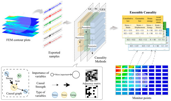
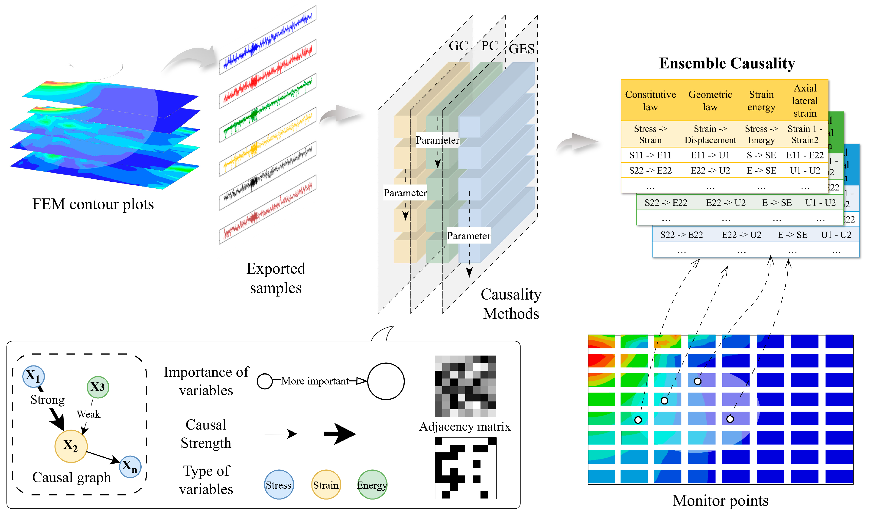
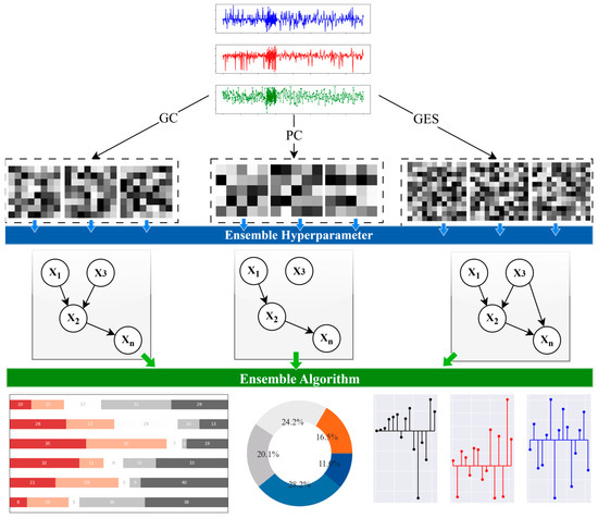
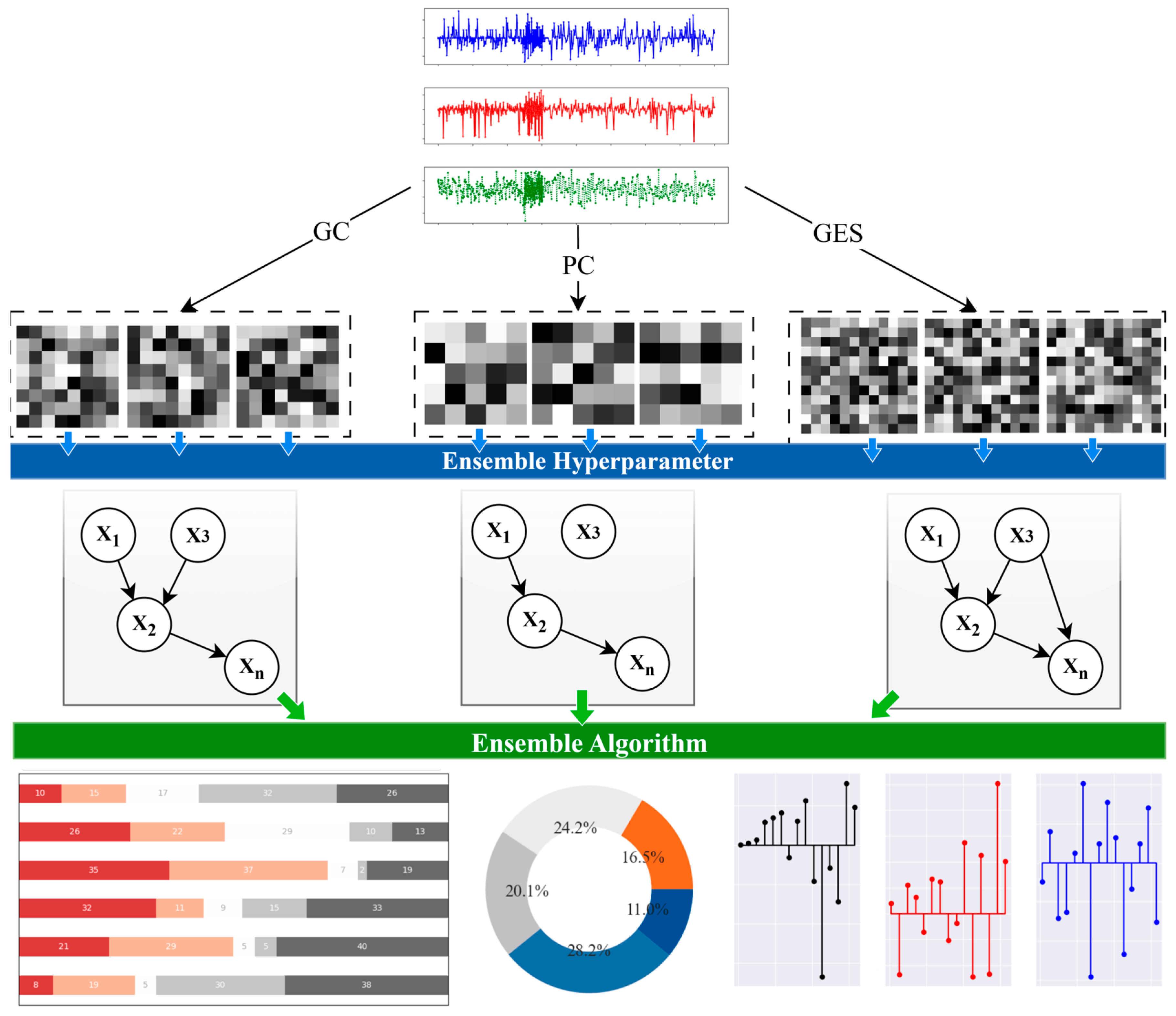
As illustrated in Figure 1, the causal discovery begins with numerical experiments involved with mechanical characteristics; namely, the Finite Element Method (FEM) is utilized to complete the mechanical process, performance testing on devices, and manufacturing technique. Then, the recorded samples of monitor points on stress, strain, energy, and displacement are exported for the preparation of causal reasoning. After employing the causality measures, graphs denoting variable importance, connection strength, and network structure are generated. Next, the outcomes in the initially derived graph across various causality measures, hyperparameters, and cases are ensembled for better understanding of typical mechanical stages within the process, influences of material property and location of monitor points.
Figure 1.
Schematic of presented causal analysis workflow.
2. Numerical Experiments
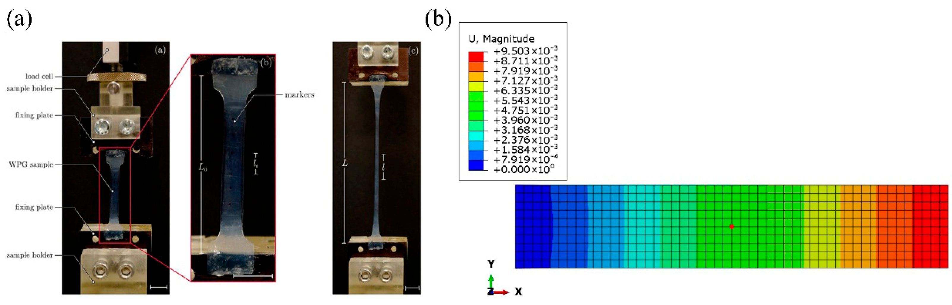
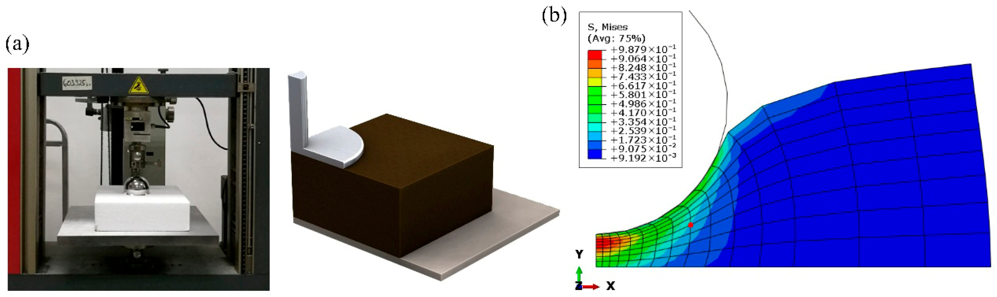
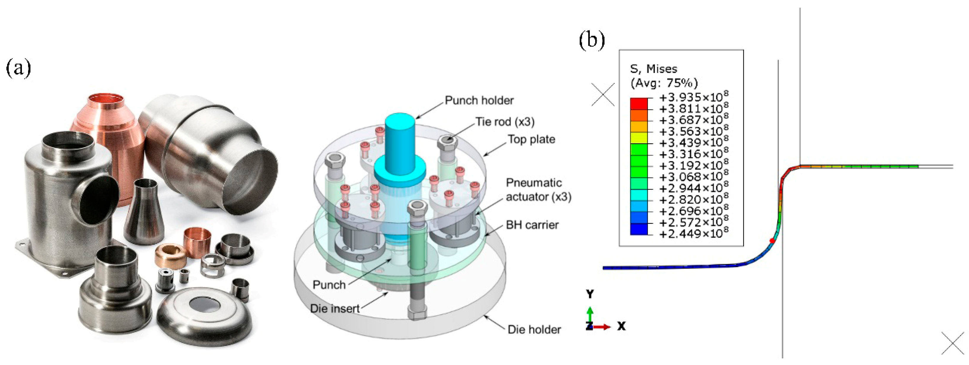
Numerical simulation experiments exhibiting concerned mechanical mechanisms and closely related to practical applications in engineering or industry are utilized. At first, the stress and strain experienced by a member due to a tension/compression load acting along its length is studied. The next case is a cylindrical specimen of an elastomeric foam, indented by a rough, rigid, hemispherical punch, showcasing how the foam-based energy-absorbing materials work in shock absorption and impact protection systems. The third case introduces a widely used manufacturing technique to get deep-drawn cups for common metals, including stainless steel, aluminum, and brass, in which a circular plate of the sheet metal is punched out of a sheet metal strip and then formed into a cup by a drawing die. All cases take the model’s central point as an example to begin the analysis, which are highlighted in the red dots in Figure 2, Figure 3 and Figure 4.
2.1. Axial Tension
The first studied case is a rectangular bar loading in tension and compression [22]. For simplicity, a 2D numerical model containing two stages is set up. The model size is 10 m high and 50 m wide with a mesh of 500 linear quadrilateral elements in type CPS4. Commonly used steel elastic properties are assumed, including a Young’s modulus of 200 GPa and a Poisson ratio of 0.25. The left boundary of the bar is fully encased, while the load is added by applying a uniform displacement in the x-direction (U1) on the right side. In the first stage, tensile force is exerted by setting U1 to 0.02, while it changes to −0.03 in the second stage to simulate the compression situation. The distribution of resultant displacement is displayed by a contour plot, shown in Figure 2b. The schematic diagram of the tensile test is presented in Figure 2a.
Figure 2.
Experiment of Axial Tension Case. (a) Axial tension experiments [23]. (b) Contour plot of displacement in numerical experiment.
2.2. Indentation Foam
In the second case, a cylindrical specimen of an elastomeric foam, indented by a rigid and hemispherical punch, is investigated [24]. Owing to the symmetry, only half of the length of the specimens is modeled [25]. The foam specimen has a radius of 600 mm and a thickness of 300 mm, meshed with 135 axisymmetric elements CAX4 described as 4-node bilinear axisymmetric quadrilateral elements. The material of the elastomeric foam is defined using experimental data in the uniaxial compression test and simple shear test. The punch is simulated as a rough spherical rigid body, with a radius of 200 mm. To account for the axisymmetric nature of the model, the bottom edge is fixed, the left side is constrained in the x-direction, and the outer boundary is free to move [26]. The contact between the punch and the foam is defined in terms of two surfaces that may interact with each other: the indent as the master surface and the piece of foam as the slave surface. A friction coefficient of 0.8 is employed to mimic the interaction.
The whole indentation process is composed of two stages. In Stage 1, the model is loaded at the top by the punch moving downward to a maximum displacement of 250 mm. In Stage 2, the punch returned to its original position, and the deformation of foam gradually recovered. The contour plot of vons of Mises is illustrated in Figure 3.
Figure 3.
Experiment of Indentation Foam Case. (a) Indentation foam experiments [27]. (b) Contour plot of vons of Mises in numerical experiment.
2.3. Deepdraw Cup
This case illustrates an important manufacturing technique, the deep drawing of a sheet metal cylindrical cup [28]. It is accomplished by one cycle of punch movement through the die and back to the original position, resulting in deformation of the blank to a desired shape shown in Figure 4. Because of the presence of elasto-plastic transformations and the non-constant boundary conditions of contact with friction, the modeling of the deep-drawing process involves more complex non-linearity [29]. In this study, a 2D axisymmetric model is chosen for showcase, in which four components called punch, die, blank-holder, and blank are created and assembled in Abaqus. Three stages are carried out to accomplish this manufacturing simulation process: Push the blankholder down and apply prescribed force; Move the punch down against the blank; Remove the contact surface and return to the original boundary.
The circular blank to be drawn has an initial radius of 100 mm and an initial thickness of 0.82 mm, with finite element meshes in 40 linear quadrilateral elements of type CAX4R. Aluminum-killed steel satisfying the Ramberg-Osgood relation is adopted for the material property of the blank. The forming load of 100 kN is applied on the blank holder in the downward direction, then transferred from the punch through the drawn part wall into the blank. Mechanical interaction between the blank and the blank holder and the die is assumed to be surface-to-surface contact formulation, by employing a friction coefficient of 0.2.
Figure 4.
Experiment of Deepdraw Cup Case. (a) Deepdraw cup experiments [30]. (b) Contour plot of vons of Mises in numerical experiment.
This article will present causal reasoning from the above cases’ experimental results. To get a deeper understanding of interested relations, the scope is narrowed down to six mechanical variables, including strain energy (SE), stress (S), strain (E or LE), and displacement (U). Here, two kinds of representations of strain (E or LE) correspond to the integrated strain measure E and the logarithmic strain measure LE provided in the FEM analysis.
3. Causal Analysis Methods
In order to illustrate the feasibility of analyzing mechanical problems through the perspective of causality, this work concentrates on three popular methods in the causal discovery field. They are not only good at uncovering cause-and-effect relationships but also visually interpretable in nature through the generated causal graph.
After employing a significance test to decide whether causality exists between and through causal analysis methods, an adjacency matrix representing a finite graph is built, in which the elements of the matrix indicate whether pairs of nodes are adjacent or not in the graph. Then, by utilizing the fundamental concept in graph theory, a Directed Acyclic Graph (DAG) with inferred causality can be drawn, which is widely used in computer science and engineering to represent dependencies and relationships [31]. A DAG is a directed graph characterized by the absence of cycles, which ensures an acyclic flow of information. In this framework, nodes represent variables and are connected by directed edges; for instance, an edge from to signifies that exerts a causal influence on .
The subsequent content in the current section introduces the employed methods: Granger Causality (GC), Peter-Clark algorithm (PC), and Greedy Equivalence Search (GES) [32].
3.1. Granger Causality
Granger Causality (GC) is a well-established causal inference method widely used in neuroscience and economics [10]. Recently, its application has expanded into industrial and engineering fields to investigate the underlying causes of physical phenomena. Conceptually, Granger-causes if forecasting is significantly more accurate when using the past values of both and (the unrestricted model) rather than the past values of alone (the restricted model). The univariate autoregressive models for variables and are defined in Equations (1) and (2) [33].
Here,represents the autoregressive coefficients, while denotes the prediction errors. For time series of length , the model order is restricted to .
If the variance of error is statistically significantly smaller for the model taking into account the variable ( different from zero) than the variance of the same model without taking into account the variable ( equal to zero), then it implies that causes .
GC is quantified using an F-test based on the logarithmic ratio of autoregressive prediction errors. Specifically, is the error variance of a model using only the history of , whereas is the error variance of a model that uses the combined history of and .
In statistical hypothesis testing, the -value measures the probability of observing the data given that the null hypothesis is true. For the GC test, the null hypothesis assumes no causal relationship, whereas the alternative hypothesis indicates the presence of causality. A -value below 0.05 typically warrants rejecting the null hypothesis, signifying a statistically significant connection. Regarding the hyperparameters of the GC method, the lag order is considered the most critical factor influencing the resulting causal structure. Therefore, is optimized by searching within the interval detailed in Table 1.
Table 1.
Hyperparameter settings in causality analysis methods.
3.2. Peter-Clark Algorithm
Causal discovery methods are broadly classified into two main categories: constraint-based and score-based algorithms [34]. Constraint-based approaches infer causal structures by evaluating conditional independence within observational data. Meanwhile, score-based methods identify the optimal causal network by maximizing a predefined scoring function over the space of possible DAGs.
The Peter-Clark (PC) algorithm is a classic and widely recognized constraint-based method [35]. It addresses this computational challenge by repeatedly testing candidate causal links conditioned on subsets of the remaining variables. Operating under the assumptions of independent and identically distributed (i.i.d.) data and the absence of latent confounders, the PC algorithm utilizes conditional independence (CI) tests to prune invalid edges. This process first establishes the undirected skeleton of the causal network, and then orients the edges to form a DAG. Because CI testing lies at the core of constraint-based methods, this study implements four distinct CI tests, which are summarized in Table 1. The pseudocode for the PC algorithm is provided in Algorithm 1 [36].
| Algorithm 1. PC Pseudocode of the Peter-Clark Algorithm |
| 1: Input: Variables |
| 2: Output: Directed acyclic graph (DAG) |
| 3: Initialize: Fully connected undirected graph |
| 4: Repeat: |
| ) do |
| exists then |
| 9: Execute the orientation rules making use of v-structures and acyclicity assumption |
3.3. Greedy Equivalence Search
In contrast to the PC algorithm, which relies primarily on statistical tests of conditional independence, score-based learning methods pair a scoring metric with a search algorithm to navigate the space of possible graphs. These methods identify the optimal causal structure by maximizing a goodness-of-fit score for a candidate graph given the observed data . A prominent example of this approach is the Greedy Equivalence Search (GES) algorithm, which performs a greedy search over the space of Markov equivalence classes, also referred to as essential graphs or completed partially directed acyclic graphs.
A score commonly used by GES is the Bayesian Information Criterion (BIC) score [37] described in Equation (4). Given a model class for each , and the data has samples, the BIC score is:
where is a hyperparameter, is the likelihood maximizer over , and the number of parameters is the number of edges in .
Another popular metric is the Bayesian Dirichlet equivalent uniform (BDeu) score [38]. It defines priors for conditional probability distributions using a single hyperparameter called the prior equivalent sample size [2], and is calculated as:
where is the number of states of node ; is the number of configurations of the parents of ; The most common implementation assumes . is the number of times in the data that took its kth value when the parents of had their jth instantiation. and .
Starting from an edge-less DAG, the GES algorithm iteratively optimizes a scoring metric through a three-phase procedure [37]:
Step 1: Evaluates all valid edge additions, executing the one that maximizes the score increase, and repeats this process until no further additions are beneficial.
Step 2: Evaluates all valid edge removals, executing the one that provides the greatest score improvement, continuing until no deletions increase the score.
Step 3: Evaluates all possible edge reversals within the Markov equivalence class, applying the one with the highest score gain, and repeats until convergence.
The outcome of the inferred graphs will be influenced by many factors, including the algorithm chosen, hyperparameter values, data size and quality, and so on. This study concentrates on GC, PC, and GES methods and selects the most critical hyperparameters to display results. Their specific ranges are listed in Table 1, and others remain at defaults as implemented.
Regarding the discretization strategy, CI tests in Chi-Square and G-Square are employed for categorical variables in PC. Besides, if the local score function is BDeu in GES, the input variables are also discrete categorical features. To convert the continuous numerical data into these required bins, a quantile-based discretization strategy is adopted. Specifically, the first and third quartiles are used as thresholds to partition the data distribution into three distinct intervals. This quantile-based approach was chosen because it ensures a balanced representation of data points across bins, making the algorithms more robust against the skewed distributions and outliers often encountered in non-linear mechanical responses.
4. Result
The implementation of the aforementioned causal analysis methods, namely, Granger Causality (GC), Peter-Clark algorithm (PC), and Greedy Equivalence Search (GES), will be shown in terms of mechanical experiments completed by numerical simulations, respectively. Especially, the point near the center of the model is investigated. The results are reported in graphical form and its corresponding adjacency matrix. Instead of presenting the raw inferred outcomes over the hyperparameters in separate causal networks shown in Appendix A, the generated graphs have been processed to mitigate the impact of hyperparameter settings. Furthermore, the importance of each variable and the strength of each causal connection can be visualized through the improved cause-and-effect diagram. The node color denotes the type of variable: “plum” is strain energy (SE), “skyblue” is stress (S), “blue” is strain (E or LE), and “darkcyan” is displacement (U). Their subsequent numbers express the direction: S11 refers to stress components in x-direction and U2 refers to displacement components in y-direction.
4.1. Axial Tension
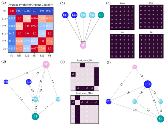
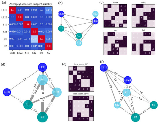
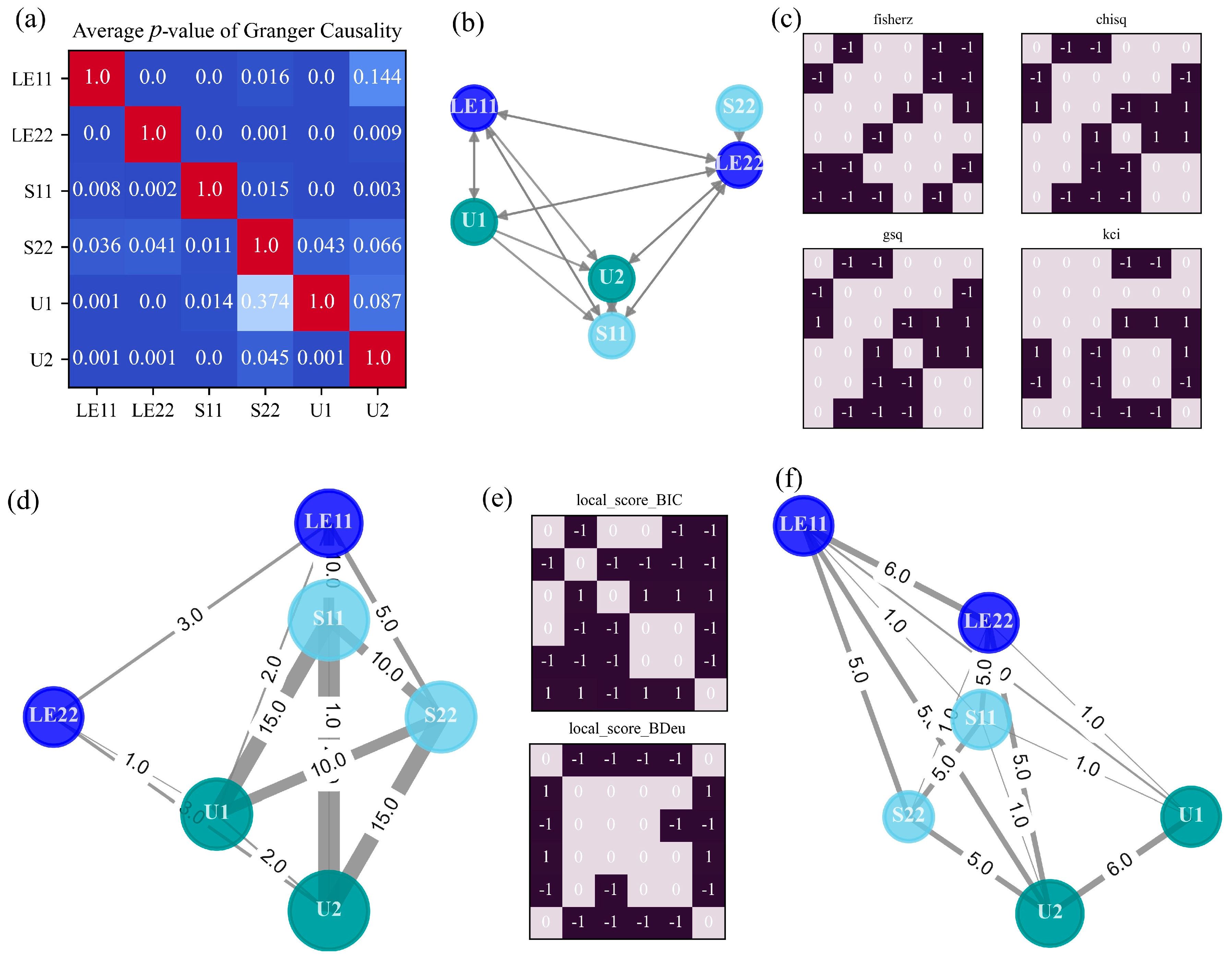
For Axial Tension Case in terms of its two stages, the results of three investigated causal methods are illustrated in Figure 5. Because the raw inferred causal networks are difficult to reveal general and scalable rules, an approximate graph is produced by taking into account several possible values of lag orders. This technique is called model averaging, returning the average output over multiple candidate outputs as determined by a single causal analysis method. It is inevitable that large inconsistencies exist among the learned outputs based on different hyperparameter values. Thus, taking the average of all the p-value matrices of granger causality test can yield a quite clear and comprehensive causal graph [39]. With the consideration of the most concerned hyperparameter ranging from 1 to 4, an averaged causal graph is derived in Figure 5b, as well as its corresponding p-value matrix in Figure 5a.
Figure 5.
Generated causal graphs and causal matrices in Axial Tension Case. (a) Averaged p-value of different lag orders in GC. (b) Causal graph by GC. (c) Adjacency matrix versus independence test method in PC. (d) Causal graph by PC. (e) Adjacency matrix versus score function in GES. (f) Causal graph by GES. The significance level is set as 0.01 for GC and 0.001 for both PC and GES.
The generated causal graph successfully identifies the interaction between strain energy (SE) and other mechanical variables such as stress (S11, S22), strain (E11, E22), and displacement (U1), but it failed to detect further associations among stress, strain, and displacement. This outcome accurately reveals a known ground truth in mechanics, where strain energy is decided by the amount of deformation or strain in a material and the applied stress:
where is the stress component and is the strain component.
Moreover, all the directions of causation are also correct in that the strain energy indeed is the result of those variables. In respect to the mechanical principle, the GC method is quite suitable for discovering the underlying rules within the tension and compression of members. It should be noted that linear dependencies dominate the relationships between material, load, and geometry in this case, so uncovering several general patterns is not surprising since GC is built on linear vector autoregressive models.
Next, the adjacency matrices calculated by PC in terms of four different CI tests are presented in Figure 5c, where and means i -> j; means ; means i <-> j. Accordingly, a causal map drawn through PC is given in Figure 5d. Similarly, a strategy needs to be adopted for balancing the discrepancy induced by selecting different CI tests. Considering that the generated graphs are rather sparse, all the possible causal links discovered by each CI test are summed up. As a consequence, a causal network capable of illustrating the connection strength is obtained, in which the thickness of the edge represents the total number of connections identified by each CI test. Moreover, the importance of a variable can be expressed by its node size in the causal graph. The size is proportional to the node degree, which denotes the number of edges adjacent to the node in graph terminology.
The energy node (SE) and the displacement node (U1) appear to play important roles in the information flow, behaving like a root or leaf node respectively, while stress (S11, S22) and strain (E11, E22) serve as intermediate nodes. As stated in the first principle-based knowledge, the displacement is directly caused by the strain, and strain is directly caused by the stress. Therefore, the indirect S→U is inferred. Apart from that, many causal connections in line with mechanical formulas have been found: strain—strain energy, stress—strain energy, S22—E22, and E11—U1.
Figure 5e,f illustrate the outcomes of GES if the BIC or BDeu local score function is selected. Similar to PC, GES shares the same rules between its adjacency matrix and causal graph. Two bigger nodes describing the deformation in x direction stand out in the causal graph: E11 and U1. Besides, there are two causal links between E11 and U1, highlighting the axial interaction between strain and displacement.
For Axial Tension Case, quite different mechanical relationships have been detected, especially between the linear method GC and the other two methods. Although the causal networks generated by PC and GES are not the same, the similarities between them are obvious: regarding strain energy and displacement as the root or leaf node in the entire network, stress and strain are located in the middle; and being able to explore the relation between stress and strain, and strain and displacement.
4.2. Indentation Foam
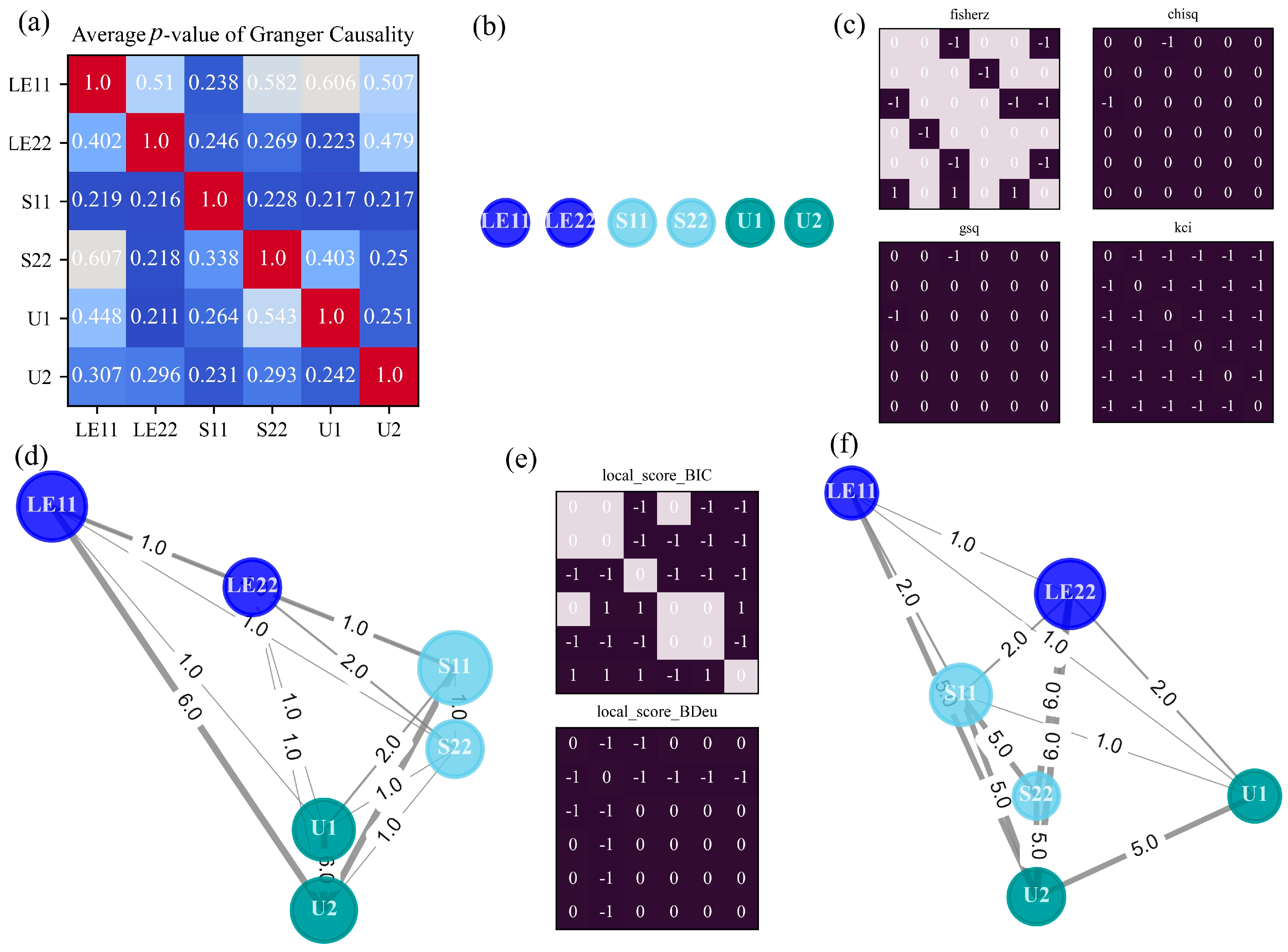
In this subsection, causal discovery for foam indentation by a spherical punch is carried out, and the results are shown in Figure 6, presenting the identical subplots for the investigated causal analysis methods as Figure 5. The element values of the p-values matrix in Figure 6a are relatively larger than the significance level, leading to a causal graph with no connecting edges. The derived blank causal diagram indicates that GC cannot capture any mechanical interactions for the current case, suggesting it is inappropriate to apply the method with the assumption of linearity to a problem involving hyperelastic material and rough contact. On the contrary, if the method is not confined to linear dependencies, plenty of causal connections are expected to be detected, as verified by the complex networks in Figure 6d,f.
Figure 6.
Generated causal graphs and causal matrices in Indentation Foam Case. (a) Averaged p-value of different lag orders in GC. (b) Causal graph by GC. (c) Adjacency matrix versus independence test method in PC. (d) Causal graph by PC. (e) Adjacency matrix versus score function in GES. (f) Causal graph by GES. Significance level is set as 0.001 for all methods.
Due to the complex mechanical characteristics of elastomeric foam indentation, PC and GES outperform GC in identifying nonlinear causal relationships, such as polynomial, exponential, and logarithmic dependencies. Specifically, this systemic nonlinearity is driven both by the hyperfoam material coefficients—derived via a nonlinear least-squares fit of the test data—and the modeled frictional contact between the punch and the foam. Compared to the linear axial tension case, both PC and GES generate denser causal networks, though they share a similar underlying skeleton. Nevertheless, distinct differences emerge between the two methods. In the PC-generated graph, mechanical responses in the x-direction (LE11, S11, U1) exhibit more connections with other nodes. Conversely, variables corresponding to y-direction deformation (LE22, U2) dominate the GES-generated network. Following skeleton estimation in PC, edge directions are determined and visualized as thicker lines (assigned an edge weight of 5). Directed connections inherently provide deeper mechanistic insight than undirected ones by explicitly specifying the cause-and-effect orientation. Notably, the directed relationships U1 -> U2 and LE11 -> U2 are correctly identified by PC. For instance, the edge U1 -> U2 indicates that displacement in the x-direction drives displacement in the y-direction, a finding consistent with the mechanical principles governing the ratio of lateral to axial strain. Similarly, the edge LE11 -> U2 reveals an indirect causal relationship that captures both the kinematic transformation from strain to displacement and the mechanical coupling between deformations in orthogonal directions. Although GES identifies a greater number of directional relationships, only two edges evaluated under the BIC score align with physical expectations: U1 -> U2 and LE22 -> U2. Based on fundamental domain knowledge, the latter relationship accurately reflects the geometric compatibility laws governing strain and displacement.
where is the strain and is the displacement.
4.3. Deepdraw Cup
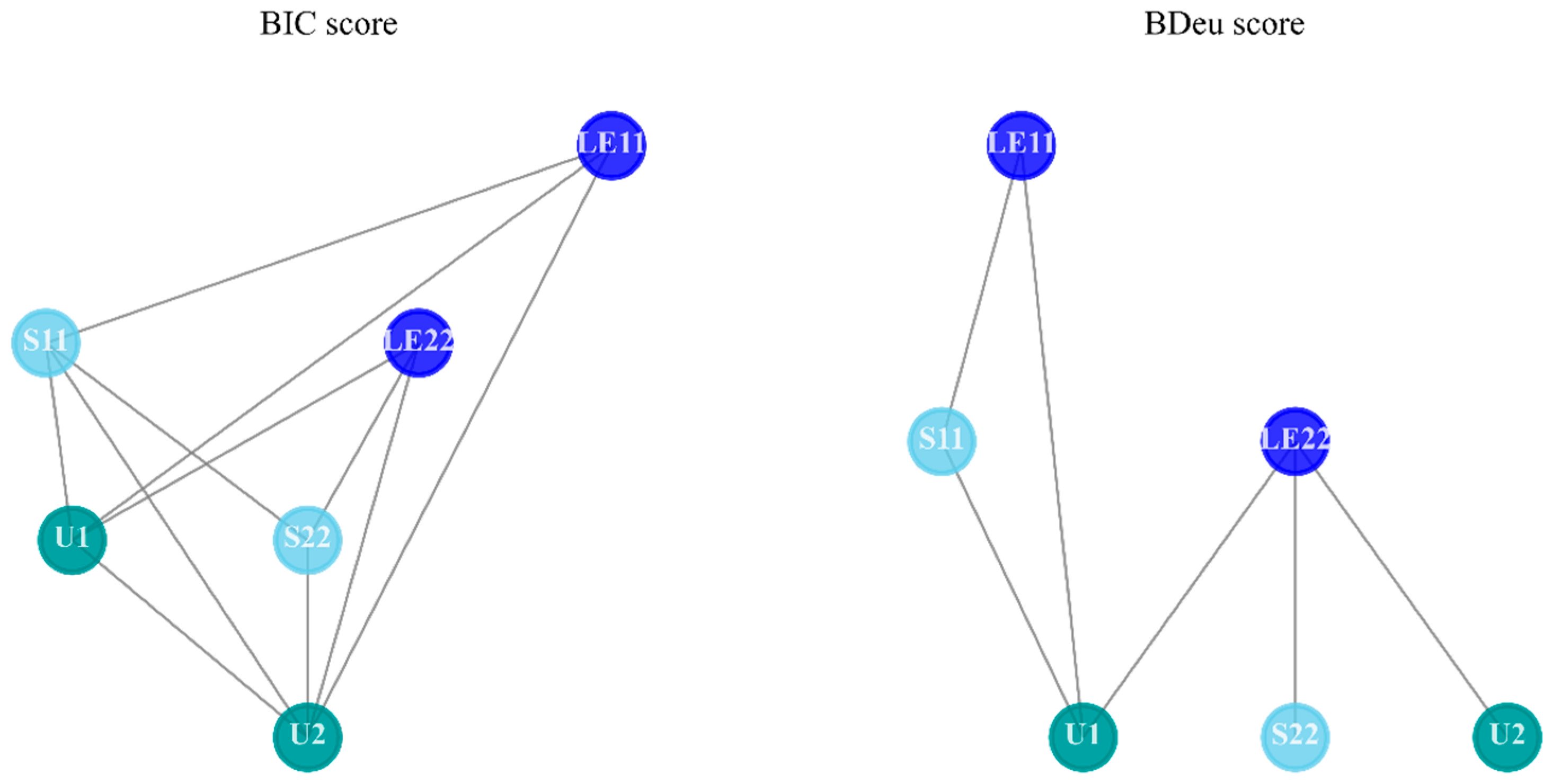
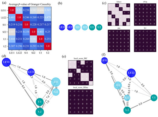
The third case illustrates the deep drawing of a sheet metal cylindrical cup, three stages to accomplish the whole manufacturing process are taken into account to learn the causal maps presented in Figure 7. It can be seen that GC draws a complicated network with dozens of connections, even bi-directional edges make up the majority. Considering the aluminum-killed steel to be processed, its stress-strain curve is defined in piecewise linear segments in the metal plasticity specification, resulting in a larger number of connections in comparison with Indentation Foam Case. However, different from Axial tension case focusing on finding causal relations with strain energy, the granger causality test turns to uncovering mechanical associations among stress, strain, and displacement. Several useful connections, such as S22 -> LE22, S11 -> LE11, and LE11 -> U1, are inferred, along with some reverse erroneous causal connections. According to the applications of GC on other problems [10], when the system under consideration involves oscillations, it does tend to produce spurious causation. As plotted in Figure A7, the oscillations in stress components can be attributed to the severely discontinuous behavior in the contact between the blank and the rigid punch, the rigid die, and the rigid blank holder.
Figure 7.
Generated causal graphs and causal matrices in Deepdraw Cup Case. (a) Averaged p-value of different lag orders in GC. (b) Causal graph by GC. (c) Adjacency matrix versus independence test method in PC. (d) Causal graph by PC. (e) Adjacency matrix versus score function in GES. (f) Causal graph by GES. Significance level is set as 0.001 for all methods.
Unlike previous cases, networks’ structures deduced by PC and GES are quite different, as demonstrated in Figure 7d,f. Moreover, although PC finds more directional links with larger edge weights, most of them make false positive errors (S22 -> S11, U2 -> LE11, U1 -> S11, U2 -> S11). In contrast to yielding many spurious causal connections, GES achieves better performance where strong causal relations in line with mechanical principles are visually displayed by thick edges: LE22 -> U2, S22 -> U2, U1 -> U2, LE11 -> LE22. Among them, S22 -> U2 is an indirect causality explaining the cause from stress to displacement in the y-direction, as the direct and precise information flow is Stress -> Strain -> Displacement. LE11 -> LE22 and U1 -> U2 reflect the cause-and-effect of deformation between axial and lateral directions. Additionally, PC intends to recognize stress and displacement as the most important variables, while the impact of each variable is difficult to tell owing to the equal size of nodes in GES’s graph.
This section offers considerable outcomes of three commonly used causal analysis methods, with regard to experiments about classical mechanical deformation, energy absorption devices, and manufacturing technique. It should be noted that the data samples used in causal analysis are extracted across the whole process in one case, and only one point located around the center of the model has been studied. In spite of the averaging or summing technique to deal with critical hyperparameters, the results obtained from different methods vary greatly, thus hard to make full use of all of them in a unified manner. In addition, most derived causal graphs are inclined to be sophisticated and difficult to conclude general rules or provide insightful suggestions. To address these issues come from the brief study on a mechanical case and the overly entangled networks, the following strategies are adopted to present further comprehensive causal analysis:
- Investigate typical stages in one case separately
- Replace the material property of the object
- Set up multiple monitor points at different locations
- Break down the causal network into isolated edges
- Integrate various causal analysis methods
5. Discussion
While the adopted methods demonstrate the capability of capturing some mechanical interactions, it should be acknowledged that this level of causal discovery tends to be the end-to-end application of algorithms, not being designed for the certain practical scenario on purpose. In fact, the direct output from the causal analysis is insufficient to draw convincing conclusions for the concerned issues in the mechanical problem. Therefore, this work develops a causal analysis workflow superior in providing insights on targeted mechanisms involved:
- Influence of stage characteristic in the same case (Refined causal mechanisms)
- Influence of material property (Constitutive law)
- Influence of monitor point location (Spatial distribution of causality)
To extend to the above concerned requirements, firstly typical mechanical stages are divided for Indentation Foam Case and Deepdraw Cup Case respectively and each stage in one case is employed with each causal analysis method for comparison. Then, the generated causal network is broken down into several isolated causal edges, enabling comprehensible research for single causal relations of interest. Next, the material of foam changes from elastic to viscoelastic to figure out what role the constitutive equation plays. To reduce the bias from a certain method, the identified causalities from different methods are then integrated versus various cases and stages. At last, causal reasoning is carried out for other monitor points set up at different locations. Figure 8 illustrates the aggregation strategy, which relying on breaking down and validating individual edges. Specifically, each causal network generated under a single condition is first decomposed into isolated directed edges (e.g., S22 -> LE22, U1 -> U2). All isolated edges from the various networks are then aggregated, with the fundamental criterion for inclusion in the final graph being statistical frequency—essentially acting as a voting mechanism across the different methods.
Figure 8.
Integrate the results of various causal analysis methods.
According to the order of the improvements mentioned above, causal inference matching mechanical process will be performed in subsequent subsections to enhance the reliability of the proposed causal analysis workflow.
5.1. Divide Typical Mechanical Stages
As stated before, the whole mechanical process in one case can be divided into several stages, where each stage presents its own characteristic. In this subsection, the studied case is the foam indentation by a spherical punch, and the whole statically deformed process is divided into two parts. The deep drawing process is the other example for showcasing the impact of typical stages on reasoning, and the details are presented in Appendix A.
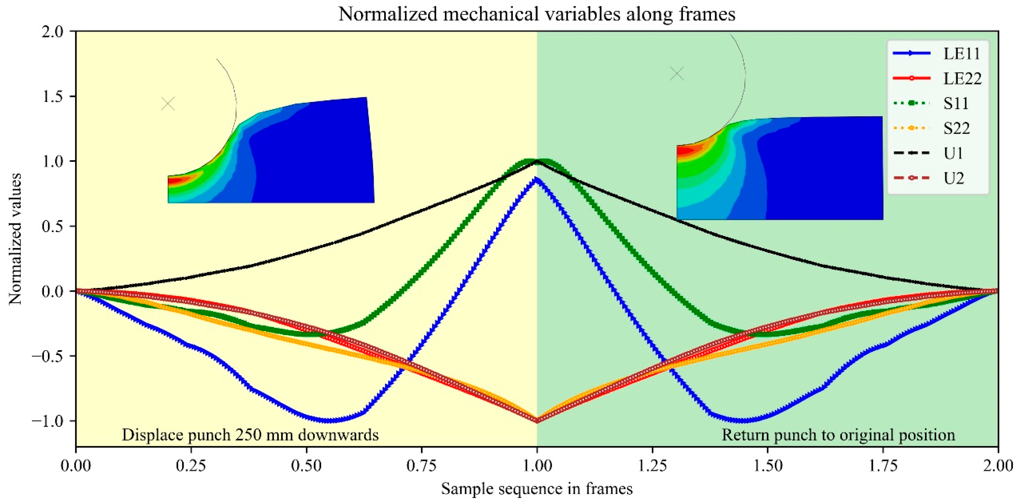
- Stage 1: Displace the punch 250 mm downwards
- Stage 2: Return the punch to its original position
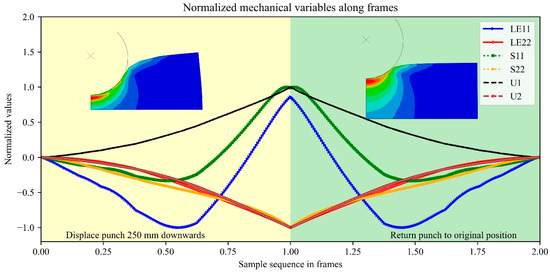
In the first stage, the load is added by punch to make severe compression of the foam, thus the foam has been subjected to large strains. In the second stage, the load is removed and the foam returns back to its original shape since elastic material is reversible. Figure 9 visualized the variation of normalized values for studied mechanical variables in these two stages. When looking at the line plots of six variables, it is easy to find that they are symmetric at the middle time, where the load disappears and the recovery begins. Hence, what the model undergoes in the second stage is relatively contrary to the first stage, as shown in the contour plots of von Mises stress distribution above. Moreover, it is easy to see that while the vertical displacement follows a simple linear path, variables such as horizontal strain (LE11) and stress (S11) exhibit obvious non-linear curves and time delays. Mechanically, these delayed responses happen since the material undergoes complex internal behaviors. Hence, these unsynchronized curves and time lags provide the essential statistical clues that algorithms require to discover the causal relationships.
Figure 9.
Sequences of mechanical variables along frames in FEM analysis using elastic properties of the foam.
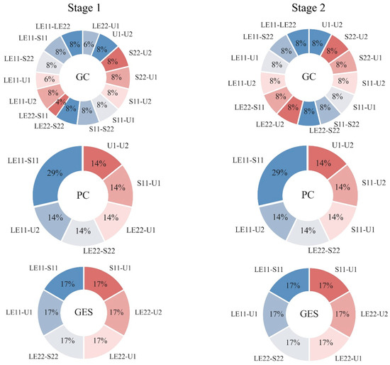
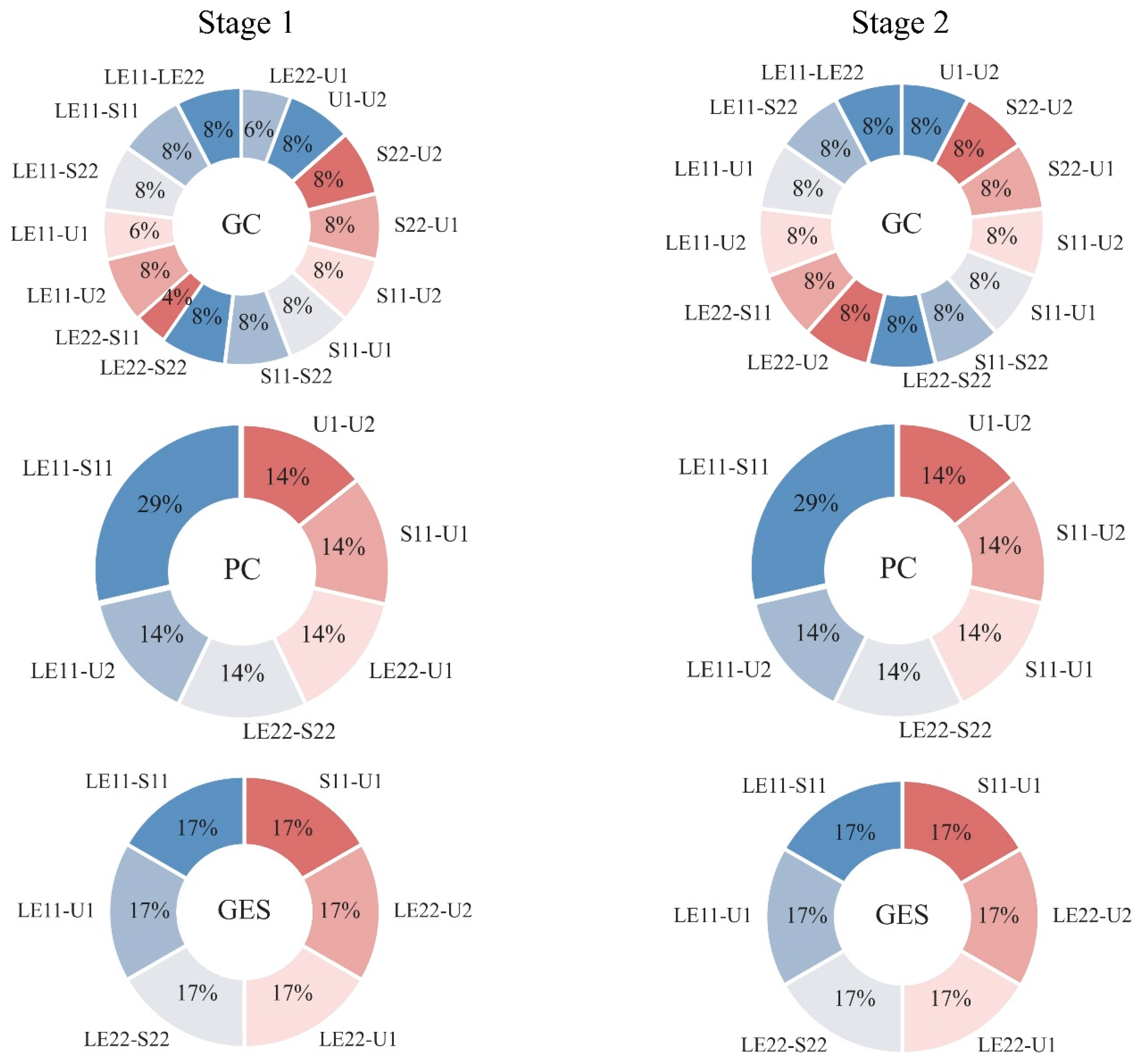
Causal inference outputs from each method in terms of two separate stages are summarized in Figure 10, illustrating the proportion of a specific causal edge’s occurrence by pie chart. To get rid of randomness and concentrate on main findings, causal edges that only appear once are neglected.
Figure 10.
Summary of causal relationships identified during the two stages of foam indentation (elastic).
Figure 10 presents six pie charts arranged in a 3 × 2 matrix. The rows represent the applied causal analysis methods, while the columns correspond to the process stages (Stage 1 on the left, Stage 2 on the right). The specific method evaluated is indicated in the center of each chart. Because the majority of causal connections identified by the Peter-Clark (PC) algorithm and Greedy Equivalence Search (GES) lack directionality, all generated graphs have been converted into undirected graphs to ensure consistency.
Notably, the results for Stage 1 closely mirror those of Stage 2 across all implemented methods. For instance, when applying Granger Causality (GC) to either stage, over ten distinct causal relationships are detected, with each comprising less than 10% of the total. Conversely, the connections uncovered by PC are concentrated into just six sectors. The causal link LE11–S11—representing the relationship between stress and strain in the x-direction—constitutes the largest proportion at 29%, while the remaining five relations account for 14% each. The outcomes of GES yield similarly identical distributions between the two stages. This striking consistency occurs because Stage 2 represents the inverse mechanical process of Stage 1: removing the applied load to allow the structure to return to its original shape. Furthermore, the analyzed data is derived from an idealized finite element analysis, which naturally produces more symmetric results than physical experiments.
Because the foam is subjected to large strains, nonlinear behavior is inevitably encountered. Consequently, GC—a method primarily suited for linear dependencies—detects numerous spurious connections and fails to isolate the dominant mechanical relationships. In contrast, PC and GES effectively capture nonlinear interactions, yielding more interpretable distributions. In these methods, six specific causal edges predominate across both stages. Most importantly, the edges denoting the constitutive law (S11–LE11 and S22–LE22) account for the majority of the discovered relationships, comprising 43% of the connections in PC and 34% in GES.
5.2. Material Property
To figure out the impact of constitutive property on causal inference, the material of the foam is changed from elastic to viscoelastic in Indentation Foam Case. Under this configuration, the displacement will reach a steady value at the stress relaxation stage, followed by a severe drop due to the impulsive dynamic load. This is followed by a rebound and then finally by a rapid decay of the subsequent oscillations due to the strong damping provided by the viscoelasticity of the foam. If the foam is viscoelastic, three stages are divided to analyze the whole process:
- Stage 1: Apply gravity force
- Stage 2: Apply dynamic load
- Stage 3: Remove the load
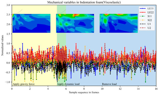
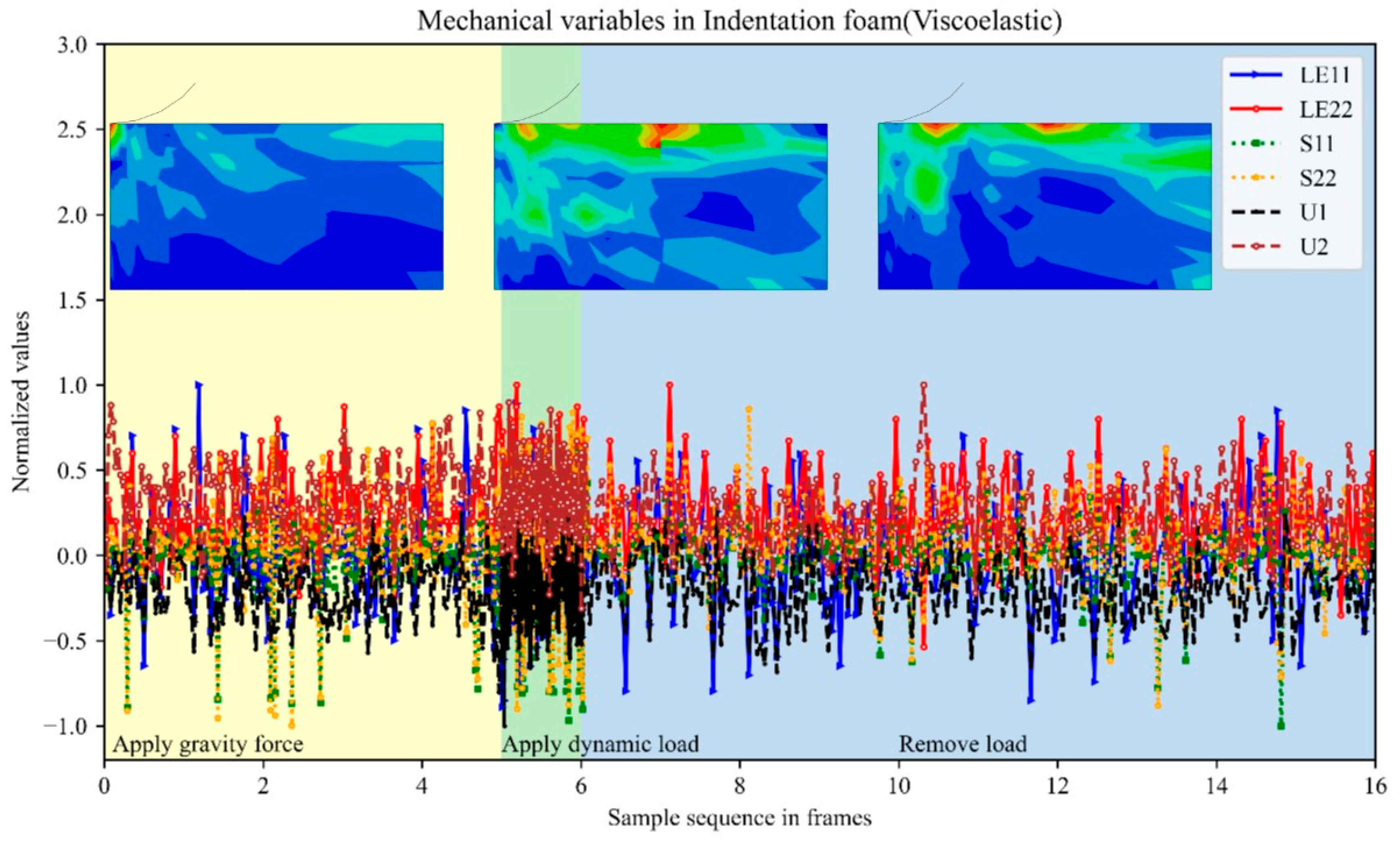
Mechanical variables of three stages in Figure 11 resemble irregular signals. The variation of each line is great and like vibration curves with huge oscillation. Besides, the contour plots of the von Mises distribution during each stage indicate the complexity of stress fields, since they are totally different from the elastic case. Such complicated and overlapped data samples are hard to analyze with the general method. As a consequence, discovering underlying causal relationships within these fluctuated line plots is demanded.
Figure 11.
Sequences of mechanical variables along frames in FEM analysis using viscoelastic properties of the foam.
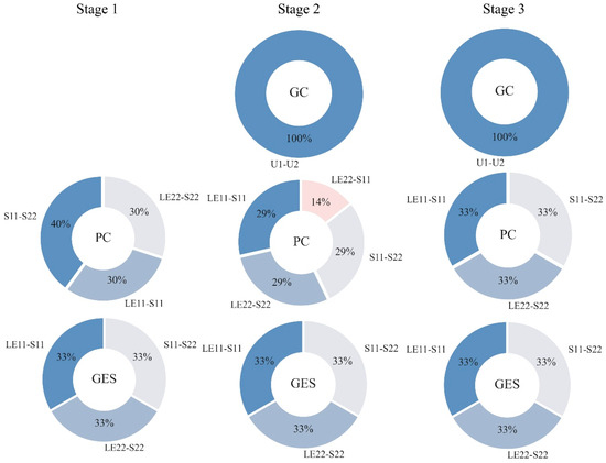
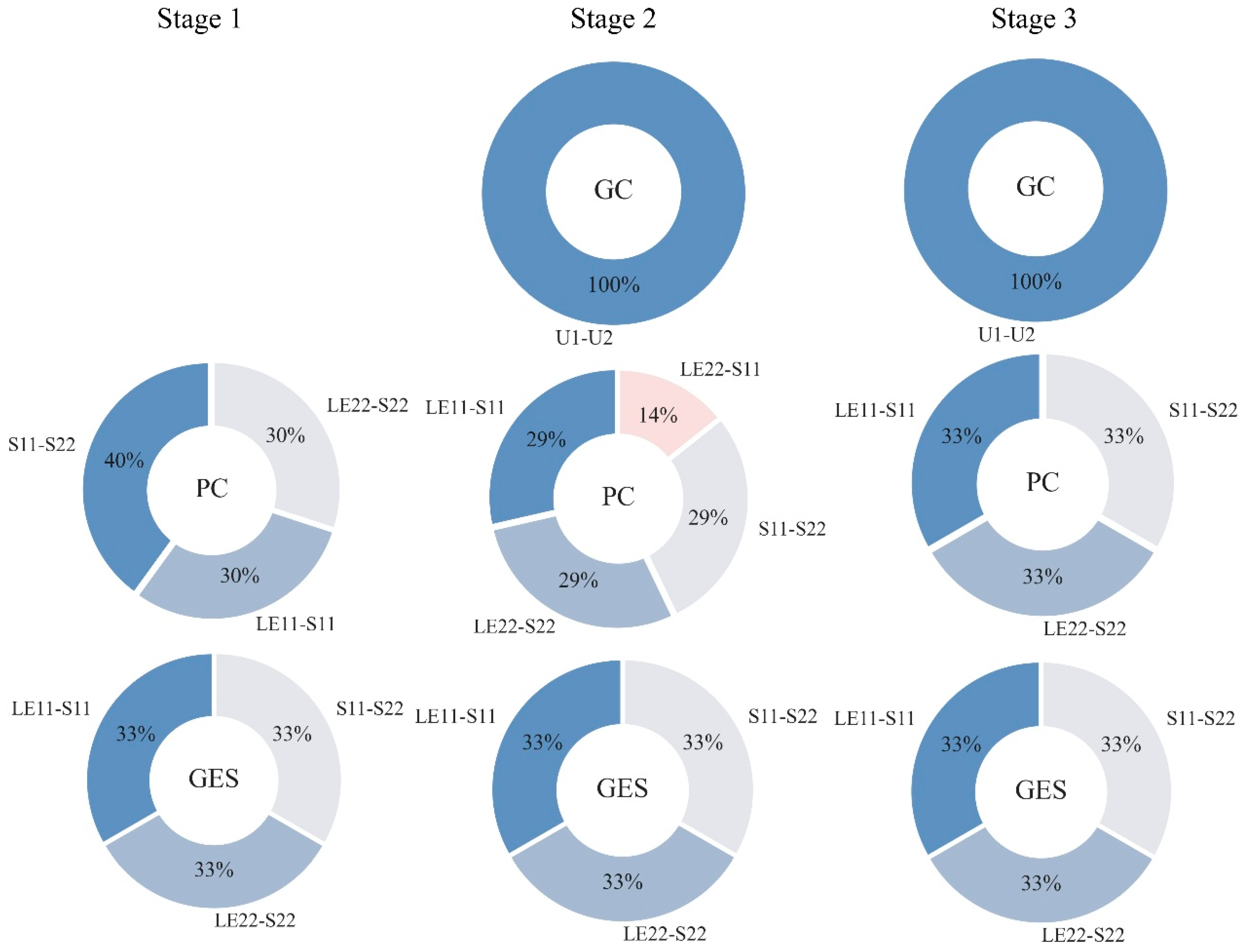
Although the variations in the mechanical variables are highly complex, the resulting causal relationships shown in the circular graphs are notably concise. Similar to Figure 10, the columns Figure 12 represent the three deformation stages, while the rows denote the causal analysis methods. Overall, the graphs indicate that the identified edges concentrate on a few specific relationships. For instance, Granger Causality (GC) detects no connections in Stage 1, and only the U1–U2 connection (representing the deformation relationship between the x- and y-directions) in Stages 2 and 3. This limited detection can be attributed to GC’s inherent difficulty in identifying strong non-linear dependencies.
Figure 12.
Summary of causal relationships identified during the two stages of foam indentation (viscoelastic).
In contrast, the PC algorithm is largely unaffected by the specific characteristics of each stage. It consistently identifies causal links between stress and strain (LE11–S11, LE22–S22) and between directional stress components (S11–S22). Similarly, the GES results remain perfectly consistent across all three stages, extracting the exact same three causal links as PC, each occupying an equal 33% proportion. Ultimately, these findings demonstrate the potential of these algorithms to successfully uncover underlying causality in complex indentation processes characterized by rapid oscillation decay, strong damping, and material viscoelasticity.
The material property is the key factor in the studied process when comparing the pie charts in Figure 10 and Figure 12. Apparently, irregular responses in viscoelastic foam hinder causal analysis to identify more kinds of relationships than the elastic one. The great impact of replacing the constitutive equation is in line with the ground truth in mechanical theory. Noticing that the interactions between stress and strain are primary causality revealed, no matter which material property is selected. Therefore, these causal analysis methods seem to be more attracted by the constitutive law since they generate isolated edges of LE11—S11 and LE22—S22 with a large proportion. Additionally, it is demonstrated again that PC and GES are inclined to generate similar results.
5.3. Integrate Results of Causal Analysis Methods
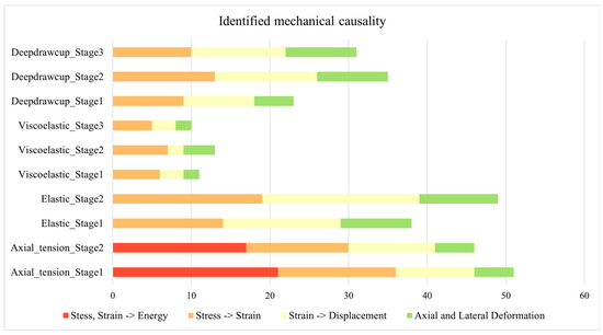
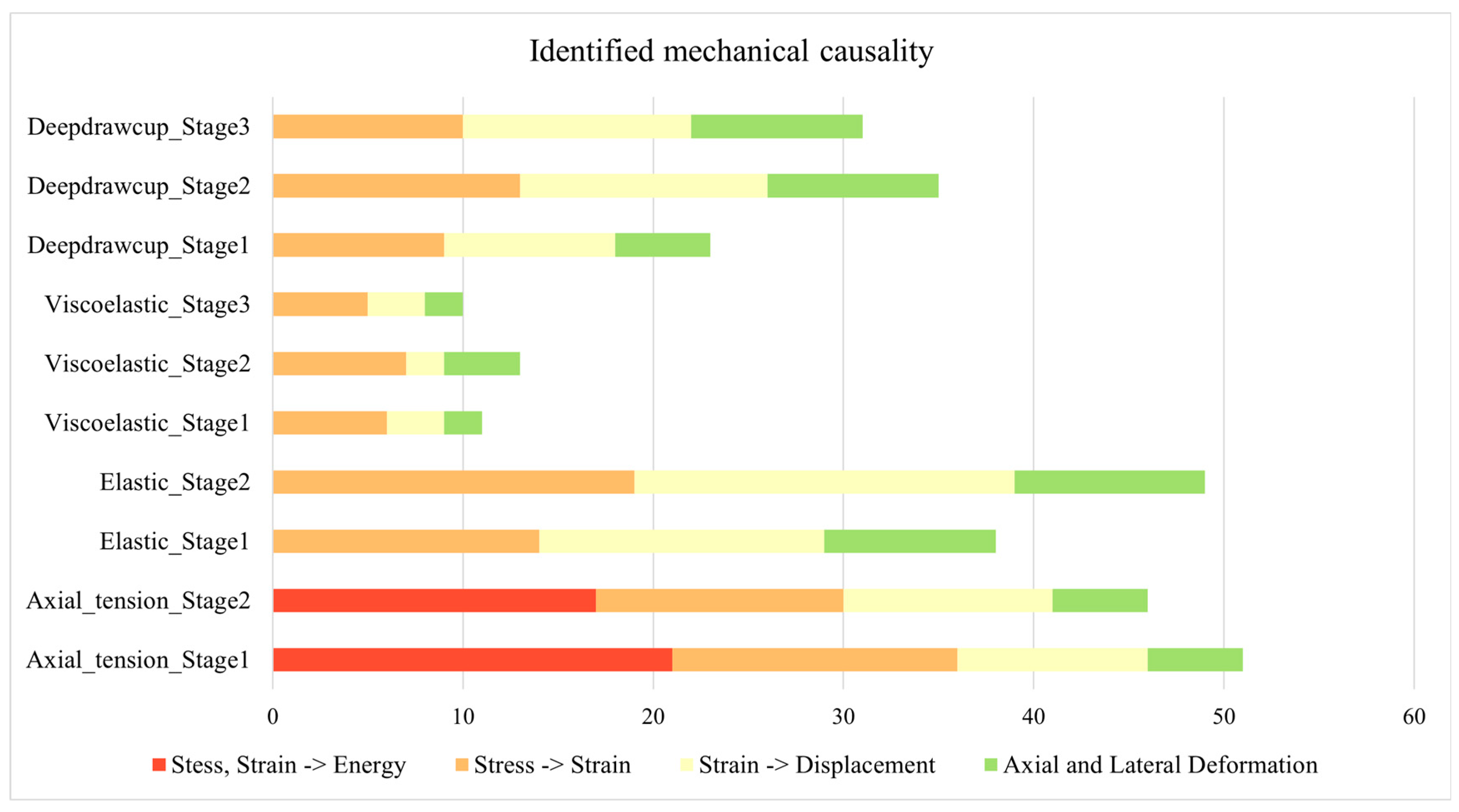
To study the types of discovered causal relations versus various cases and stages, the number of identified causalities with various methods is summed up to diminish the impact of each method’s own property, as shown in Figure 8. In addition, the desirable results focusing on the basic mechanical principles are also concluded. Specifically, by comparing the studied cases (Axial tension, Indentation foam, and Deepdraw cup) and their variants and stages, the underlying mechanisms of strain energy, constitutive law, geometric law, and deformation in orthogonal directions hidden within ten application scenarios are discussed.
According to the statistical results of causal edges in Figure 13, the number of causal relations reaches a fairly high value around 50 in Axial Tension Case and Indentation Foam Case (elastic), in which linear-elastic material is adopted. Therefore, it is easier for the employed methods to find causality. If the material changes to viscoelastic in the Indentation Foam Case, only around 10 edges are detected owing to the quite irregular trend in curves. Moreover, causalities related to energy have the largest proportion in both Stages 1 and 2 in Axial Tension Case, while causal analysis methods show little interest in detecting the associations between axial and lateral displacement in this case. Moreover, the mechanical interactions on Stress—Strain—Displacement, referring to the bar in orange and yellow, are dominant in this stacked bar chart. Unlike other cases indicating uneven distribution across various mechanical mechanisms, uniformly distributed counts are displayed in the Deepdraw Cup Case in Stages 2 and 3. This can be explained by the extreme deformation of metal during the deep drawing process, causing great variation in strain and displacement easily to be captured by causal reasoning.
Figure 13.
Number of types of mechanical causal effect identified in varying cases and stages.
5.4. Influences of Monitor Point Location
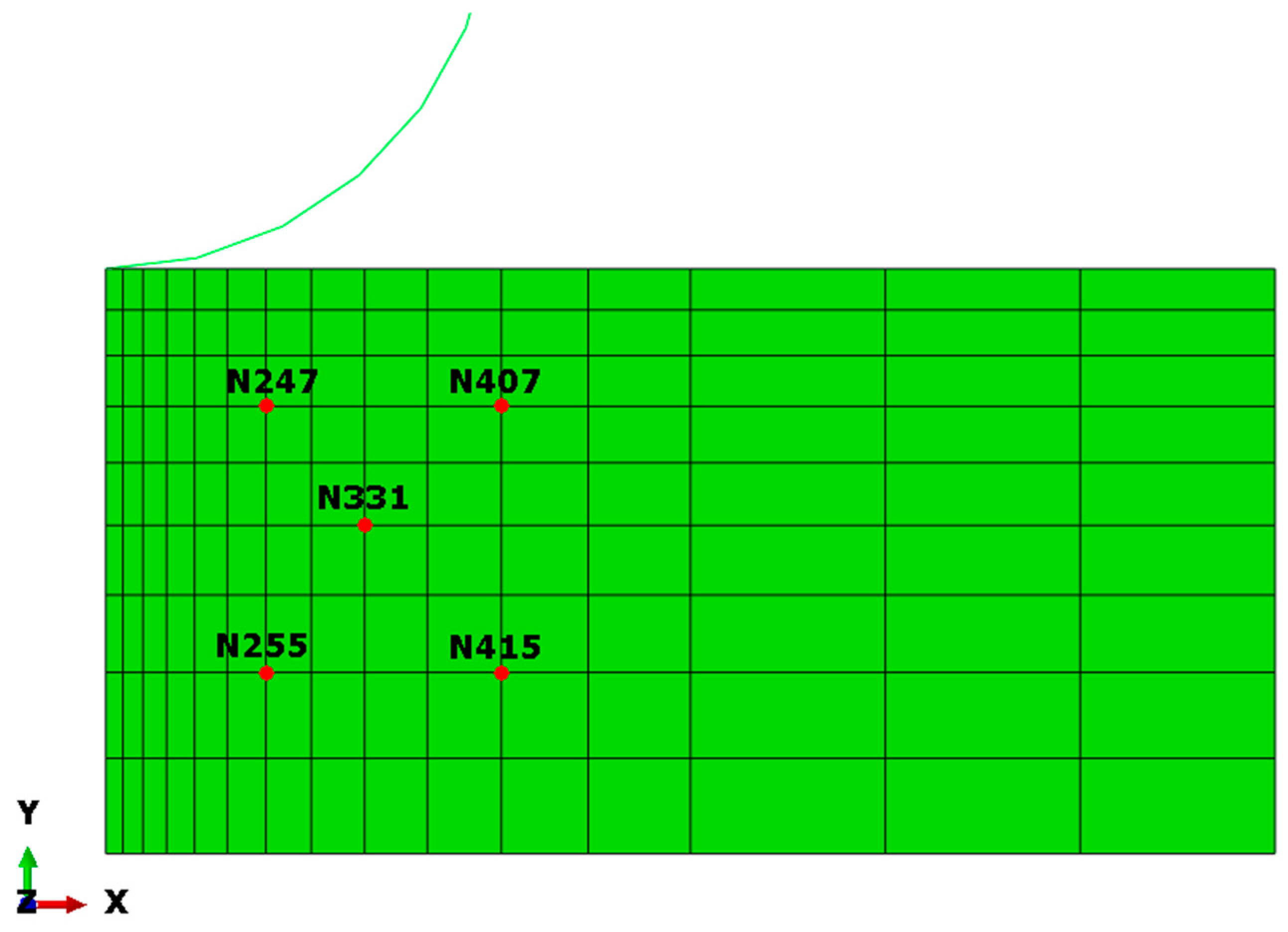
Based on the preliminary study, the proposed workflow is capable of discovering interest mechanisms. However, the revealed causality merely comes from the center point in the model. Whether the inferred causality will change with different locations of the monitor point remains a question. To verify whether this workflow can be extended to other positions, several new monitor points have been set up around the center point. Consequently, spatial distribution of causality is taken into consideration.
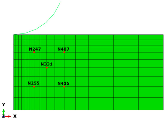
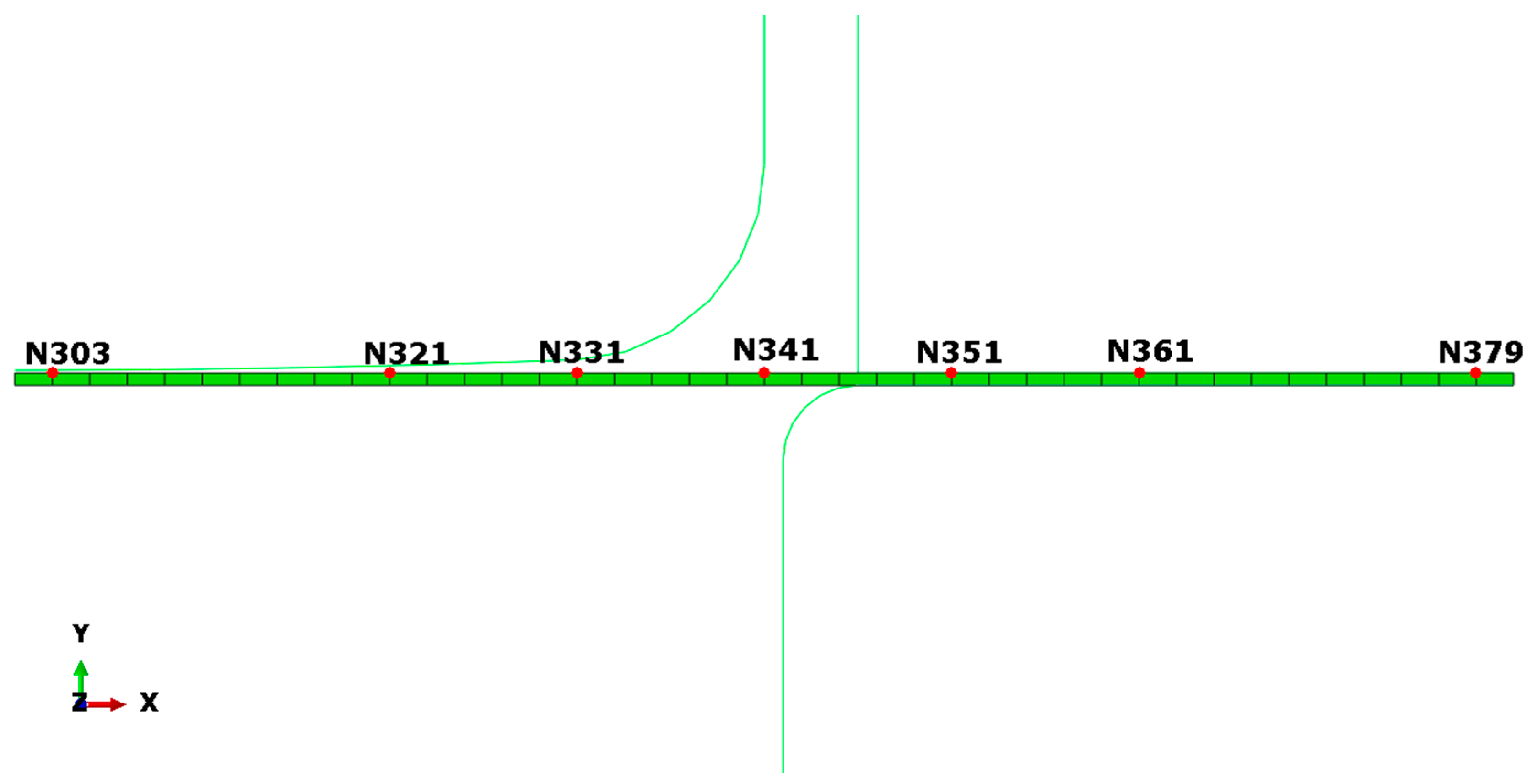
In detail, four nodes around Node 331 are added in Indentation Foam Case (viscoelastic). Six nodes located on either side of Node 341 are considered in the Deepdraw Cup Case. Both of the monitor points’ locations in two examples are given in Figure 14 and Figure 15. From the perspective of space distribution, the samples collected over time are under investigation again to support the scalability of current causal analysis. Besides, the discrepancies among the deduced connections in regard to the location of the investigated point will be revealed, providing suggestions on determining preferred monitor positions in the geometric model.
Figure 14.
Location of monitor points in Indentation Foam Case (viscoelastic).
Figure 15.
Location of monitor points in Deepdraw Cup Case.
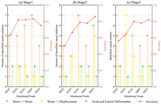
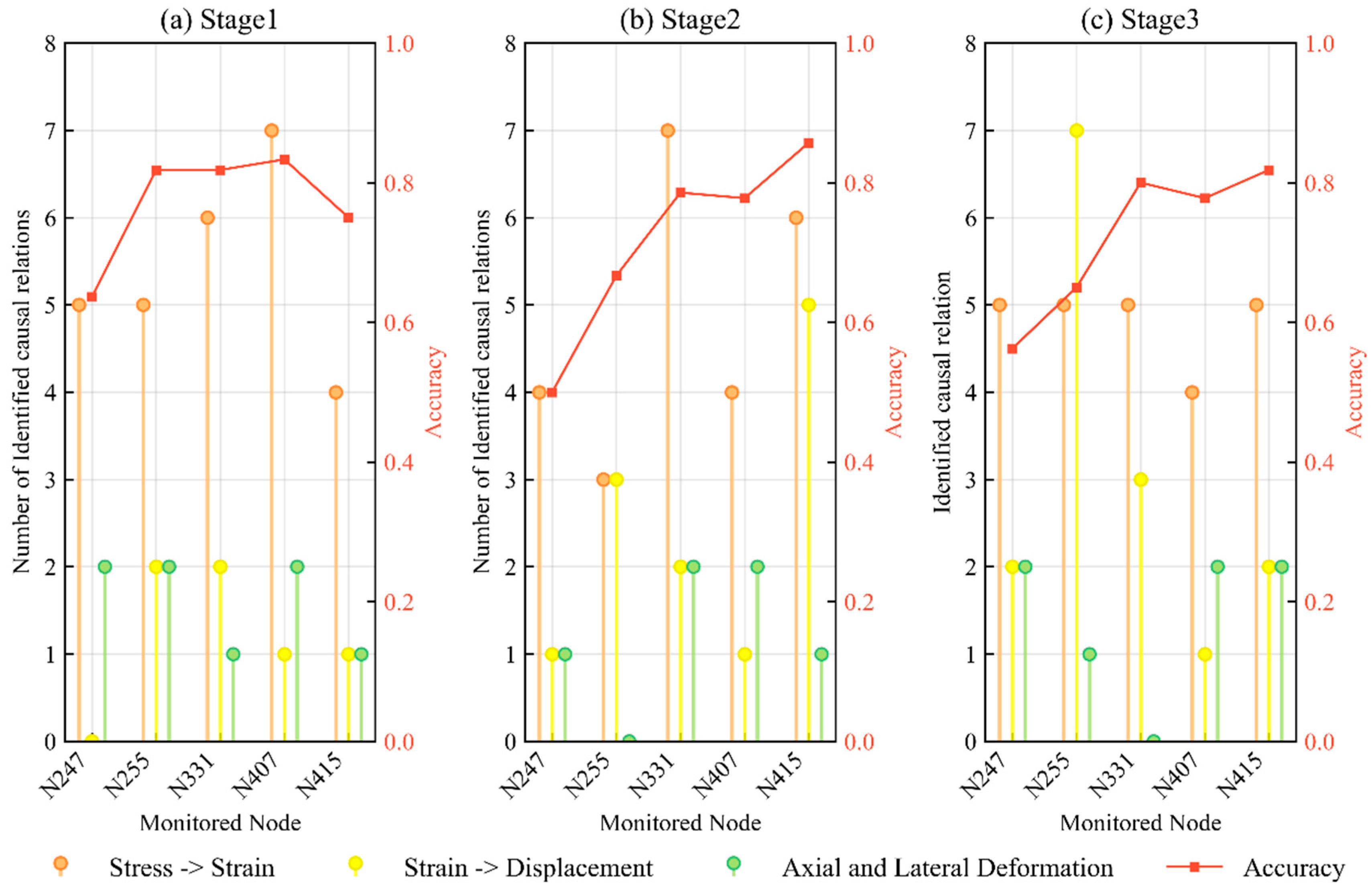
Stem plots in Figure 16 correspond to three stages in Indentation Foam Case. The number of identified causal relations in different nodes is presented along the horizontal axis, where different colors stand for the type of mechanical principle. To evaluate the correctness of causal discovery and exclude spurious links, the accuracy of causal analysis is plotted in red lines on the top of the stems. To be specific, it is the percentage of correctly identified causality among the total founded. Most points get prediction accuracy in 60~90%, indicating the feasibility of finding causality through these popular methods in causal inference fields. The points that get lower accuracy are Node247 and Node255, suffering much more deformation when the punch is compressing the foam. Thus, it is reasonable to apply it on nodes not very close to the load, namely, the punch. Moreover, the orange stem reveals the most frequently identified connection, meaning the constitutive law dominates across the nodes and the stages. Also, the difference in orange stem among nodes in different locations is small in Stage 3 and larger in Stages 1 and 2. The most influenced type of relationship is the yellow stem denoting the mechanical principle between strain and displacement. Actually, the instability of detected causality in different locations is primarily due to the significant fluctuations and uncertainty in the collected data, as shown in Figure A7. On the contrary, the relation between two directional deformations seems to be less affected by the position. Briefly, even handling quite irregular samples recorded in mechanical processes, many useful causal relations can still be explored with more discrepancies in different locations.
Figure 16.
Number of identified mechanical causal relations in Indentation Foam Case using viscoelastic properties. (a) Stage 1 (b) Stage 2 (c) Stage 3.
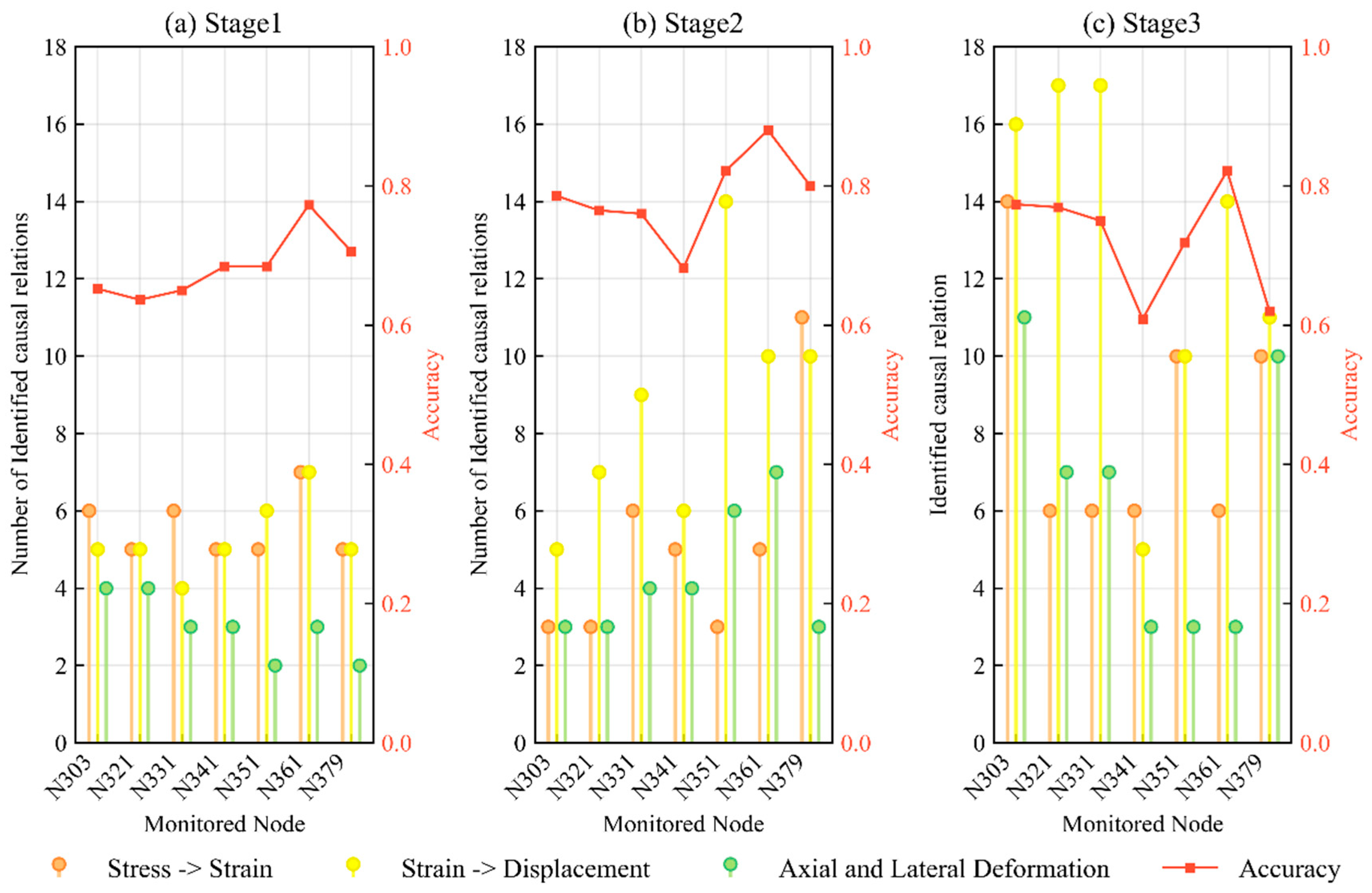
When inspecting the results in Deepdraw Cup Case in Figure 17, the accuracy of seven monitor nodes in most situations exceeds 70%, showing more reliable results than that in Indentation Foam Case. In regard to Stage 1, the number of different types of causal relationships is nearly consistent. This is because only prescribed force is applied at the beginning, so mechanical variables remain virtually unchanged. However, when the deep drawing process goes to the second stage, the height gap between stems denoting seven monitor nodes is evident, especially for Strain—Displacement. On the one hand, there has been severely discontinuous behavior in frictional contact in Stage 2. On the other hand, the contact situation of points in different positions is totally different throughout the entire stamping process. Thus, oscillations happen in the data samples, leading to unstable causal findings in different locations. At the last stage, the total number of identified causal relations increases, and there are still variations in the height of stems from Node303 to Node379.
Figure 17.
Number of identified mechanical causal relations in Deepdraw Cup Case. (a) Stage 1 (b) Stage 2 (c) Stage 3.
Noticing that the geometric distance between these seven nodes is quite large, spanning nearly the entire length of the blank. Thus, even if the compared nodes are far away from each other, the employed methods can still achieve similar results. In other words, the cause-and-effect relations inferred from one node can be extended to other nodes, since the primary causal relationships identified are in accord with each other.
Through these two studied cases, it can be concluded that it does have some influence if another location is selected. Sometimes, the nodes in various locations of the material undergo a totally different process. The results of causal discovery greatly depend on whether the node is near the fixed boundary, near to the applied load, or in contact with friction.
Besides, when facing problems in highly nonlinear, noisy, or discontinuous systems such as the strong damping by the viscoelastic property of a foam, the rapid decay of oscillations, or the severe deformation of metal material, the proposed approach still requires improvement to cover other problems with different underlying mechanical phenomena or data properties.
In this study, the challenge of scalability in analyzing massive raw networks is addressed through the refined workflow of separating typical stages. It is observed that decomposing complex processes is necessary not only for computational efficiency but for revealing the amazing consistency of causal connections across forward and reverse deformation processes. Additionally, the large discrepancy of causality found near fixed boundaries or friction zones indicates that spatial distribution is a critical factor often overlooked in purely data-driven approaches. Consequently, these beneficial conclusions open new research directions for developing hybrid frameworks, where constitutive properties and boundary conditions serve as priors to refine causal inference in equipment maintenance.
While this study successfully demonstrates the theoretical viability of causal discovery using deterministic FEM data, applying this framework to real-world scenarios will introduce complexities such as sensor noise and experimental uncertainties. Further investigation can incorporate quantitative sensitivity analyses to evaluate how reliably causal analysis can distinguish spatial boundary effects under varying noise levels. Validating the workflow against noisy, real-world experimental data remains a critical next step for translating this theoretical framework into practical engineering applications.
6. Conclusions
This study demonstrates the effectiveness of causal discovery in revealing underlying mechanical mechanisms within complex dynamic processes. Representative cases, such as the tension and compression of members, energy absorption devices, and metal forming techniques, are investigated. Furthermore, to overcome the limitations of existing methods in extracting general rules from entangled raw networks, an improved workflow designed to identify target causality is developed. By applying specific strategies to reveal mechanical interactions, this workflow enables the investigation of refined causal mechanisms across different process stages, the impact of constitutive laws, and the spatial distribution of causality. Based on numerical experiments, several key conclusions are drawn:
- Separating typical stages is necessary for causal reasoning in complex dynamic processes. Notably, a remarkable consistency in causal connections is observed between forward and reverse deformation processes. Additionally, even when applying the same causal analysis method, the proportion of isolated causal edges varies depending on the specific characteristics of each stage.
- Constitutive properties significantly impact causal inference. Regardless of the selected material behavior (e.g., elastic or viscoelastic), the mechanical interactions between stress and strain consistently emerge as the primary detected causality.
- The spatial location of monitor points heavily influences causal discovery. Specifically, significant discrepancies in the identified causality occur when nodes are situated near fixed boundaries, applied loads, or frictional contact zones.
- Granger Causality is highly suitable for extracting underlying rules dominated by linear dependencies among material, load, and geometry. Conversely, the Peter-Clark algorithm and Greedy Equivalence Search outperform Granger Causality in identifying nonlinear causality associated with metal plasticity, severe contact discontinuity, impulsive dynamic loads, or damping phenomena.
By demonstrating that statistically deduced cause-and-effect relationships align with known governing equations, this study validates that underlying mechanical rules can be successfully extracted purely from data. Furthermore, the proposed statistical causality framework can be extended to complex, real-world problems where the underlying governing equations are entirely unknown, excessively difficult to formulate, or computationally prohibitive to solve.
Future Work
The current implementation can be extended in various directions, particularly around causal networks, mechanical characteristics, and causality measures. In this study, the original complicated network is broken down into isolated edges to extract cause and effect, while graph simplification techniques can be used to simplify complex graphs, enhancing visualization and improving analysis. Besides, it would be beneficial to account for other mechanical characteristics such as strength, ductility, hardness, and toughness, allowing for better understanding of the role of constitutive law in dynamic systems. Moreover, more rigorous examination of how spatial sampling strategies impact causal discovery is necessary to provide sufficient and unbiased results. Apart from constraint-based algorithms and score-based algorithms, it is looking forward to utilizing deep neural networks to solve the problem of causal learning that involves a large number of variables.
Funding
This research was funded by National Natural Science Foundation of China, grant number 12202077.
Institutional Review Board Statement
Not applicable.
Informed Consent Statement
Not applicable.
Data Availability Statement
The data that supports the findings of this study are available on request from the corresponding author, upon reasonable request.
Conflicts of Interest
The author declares no conflicts of interest.
Appendix A
Raw inferred causal networks versus hyperparameters
The appendix presents the raw inferred outcomes over the hyperparameters in separate causal networks. Except for the causal analysis method itself, the derived outcomes are also sensitive to the choices of hyperparameters. Using the first stage in Axial Tension Case and Indentation Foam Case, the influences of causal measures and their hyperparameters are provided.
Casual graphs of Granger Causality versus lag order ranges from 1 to 9 are given in Figure A1. Obviously, the derived networks vary greatly with lag order. Besides, if the lag order is larger than 6, the structure of the generated graphs becomes stable and sparse. This phenomenon is more significant in the Indentation Foam Case shown in Figure A4. No causal relationship is detected in the last three subplots, while a rather dense network is generated as the lag order equals 1. Since there are lots of causal paths among nodes within one graph, it is hard to directly extract useful causal relationships, let alone to identify the category of principles of mechanics. When comparing the outcomes of GC in terms of these two examples, the advantage of applying GC to linear problems becomes apparent in that it is inclined to identify correct cause and effects. Meanwhile, the weakness of GC in dealing with nonlinearity is shown in Figure A4.
Figure A1.
GC generated causal graphs versus lag orders in Axial tension (Stage 1).
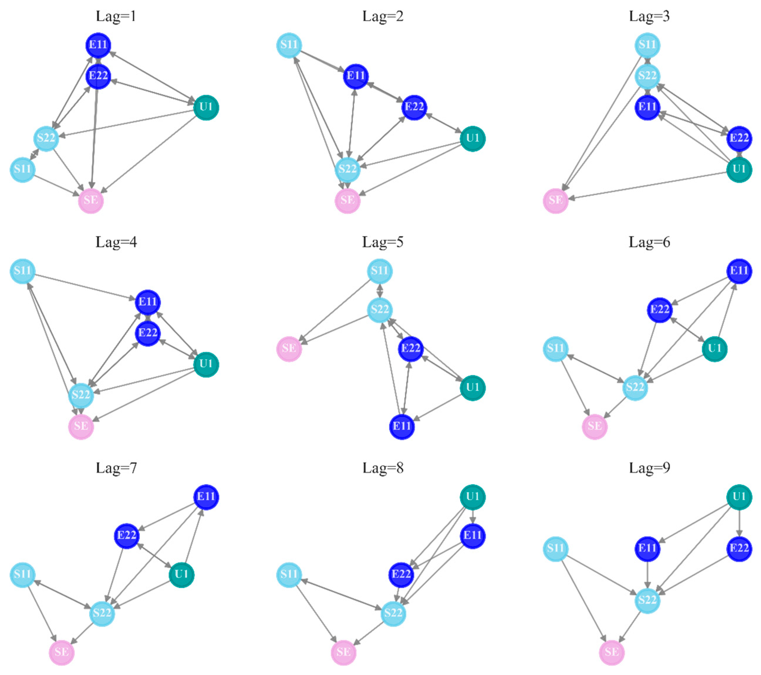
Figure A2.
GES generated causal graphs versus score functions in Axial tension (Stage 1).
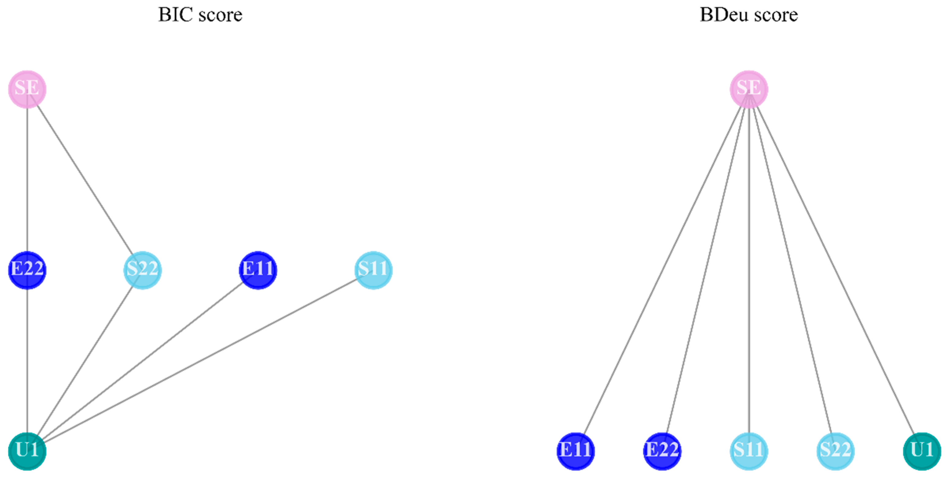
Figure A3.
PC generated causal graphs versus independence test methods in Axial tension (Stage 1).
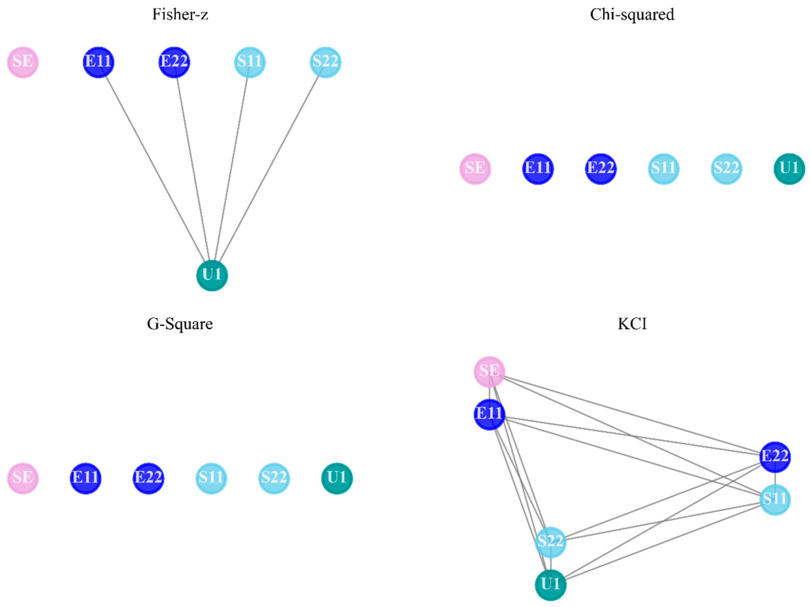
Similarly, the outcomes of PC change with the type of independence test. The kernel-based test intends to find lots of causal links, as shown in Figure A3 and Figure A5. Moreover, both Chi-squared and G-squared tests are more likely to recognize fewer edges among nodes. For GES, if the local score function is set as BIC, a denser causal map is generated than that of BDeu. As stated before, PC and GES outperform GC in the Indentation Foam Case, as they recognize more reasonable connections.
Figure A4.
GC generated causal graphs versus lag orders in Indentation foam using elastic properties (Stage 1).
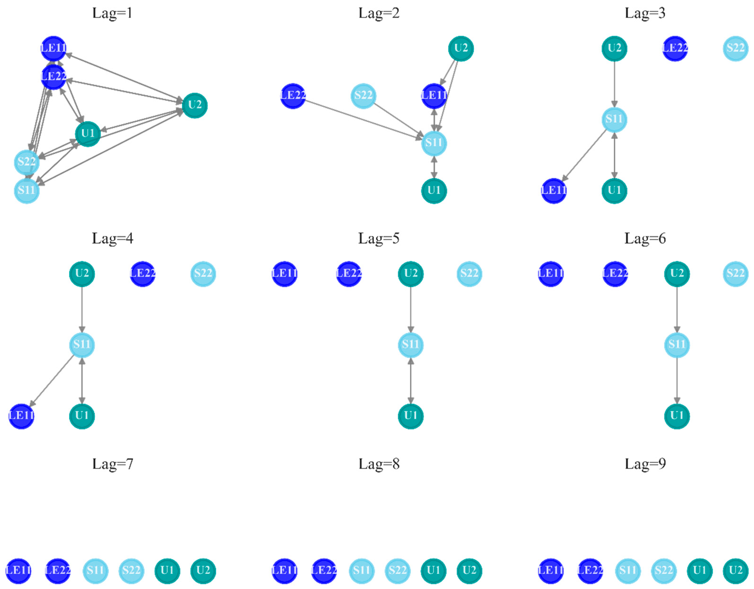
Figure A5.
PC generated causal graphs versus independence test methods in Indentation foam using elastic properties (Stage 1).
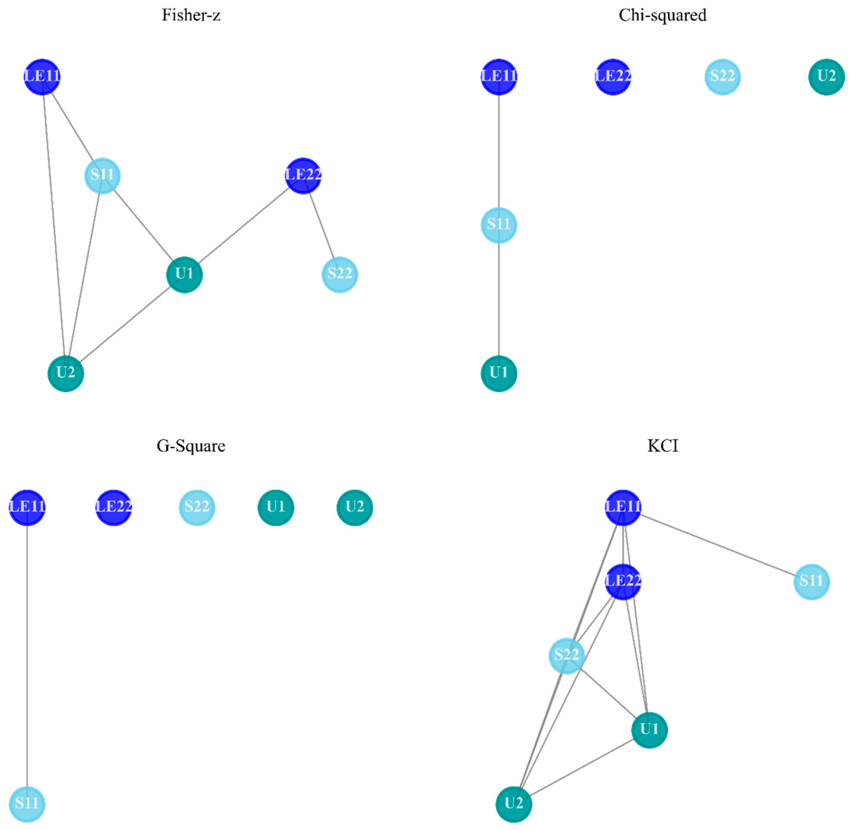
Figure A6.
GES generated causal graphs versus score functions in Indentation foam using elastic properties (Stage 1).
The deep drawing process is the other example for showcasing the impact of typical stages on reasoning. To complete this metal forming technology, three stages need to be conducted in the simulation experiment:
- Stage 1: Push the blankholder down and apply the prescribed force
- Stage 2: Move the punch down against the blank
- Stage 3: Remove contact surface and return to original boundary
The differences among three stages are shown by plotting investigated mechanical variables in Figure A7. At the beginning, the prescribed force is applied, the blank is positioned on top of the die, and the blank holder is in touch with the top surface of the blank. Correspondingly, these settings will result in little effect on the mechanical response, as plotted in Stage 1. Next, a punch is moved against the blank, which is drawn into the die in Stage 2. The metal material undergoes severe deformation to form the cup during Stage 2, and the mechanical variables change evidently along the time frame, even great fluctuations occurred in S22. At last, the contact surface is removed and the boundary is replaced in Stage 3.
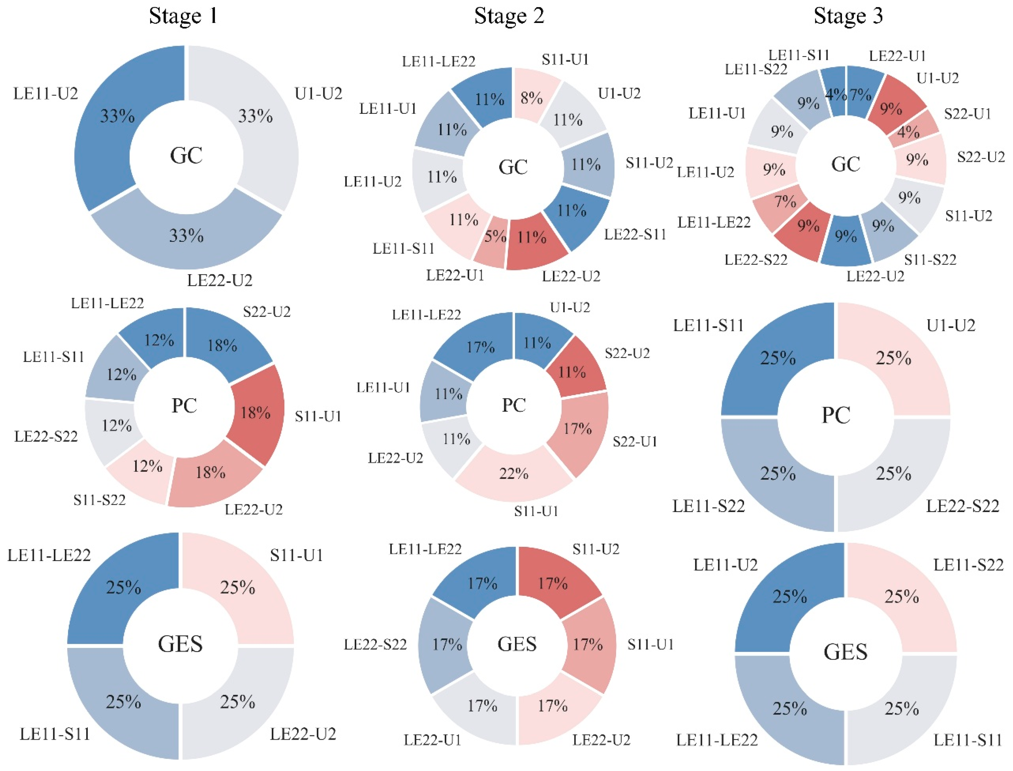
The statistical results of founded causality in the Deepdraw Cup Case are presented in Figure A8. One might find that nine subplots are different both across rows and columns, suggesting the discrepancy among types of stages and causal measures. In Stage 1, the prescribed force is applied, and little change can be found in the line plot in Figure A7, so few links are detected. The punch is moving down in the next stage, and the blank has severe deformation when it is in frictional contact with the punch and the die, leading to oscillations in the S11 and S22′ curves. As a result, diverse causal edges are captured in Stage 2 due to the significant mechanical responses of the metal material. After removing the contact surfaces and replacing the boundary, the stress curves exhibit a linear tendency in Stage 3. Thus, lots of different categories of relations have been detected by GC, in contrast to fewer sections in PC and GES’s pie chart. Considering that PC and GES have better performance in finding non-linearity than GC, the proportion of outcomes of these two methods in Stage 2 are more convincing. For instance, the resulting LE11—LE22 and LE22—U2 connections are detected by both methods, keeping in line with the ground truth on deformation rules.
Figure A7.
Sequences of mechanical variables along frames in FEM analysis in Deepdraw Cup Case.
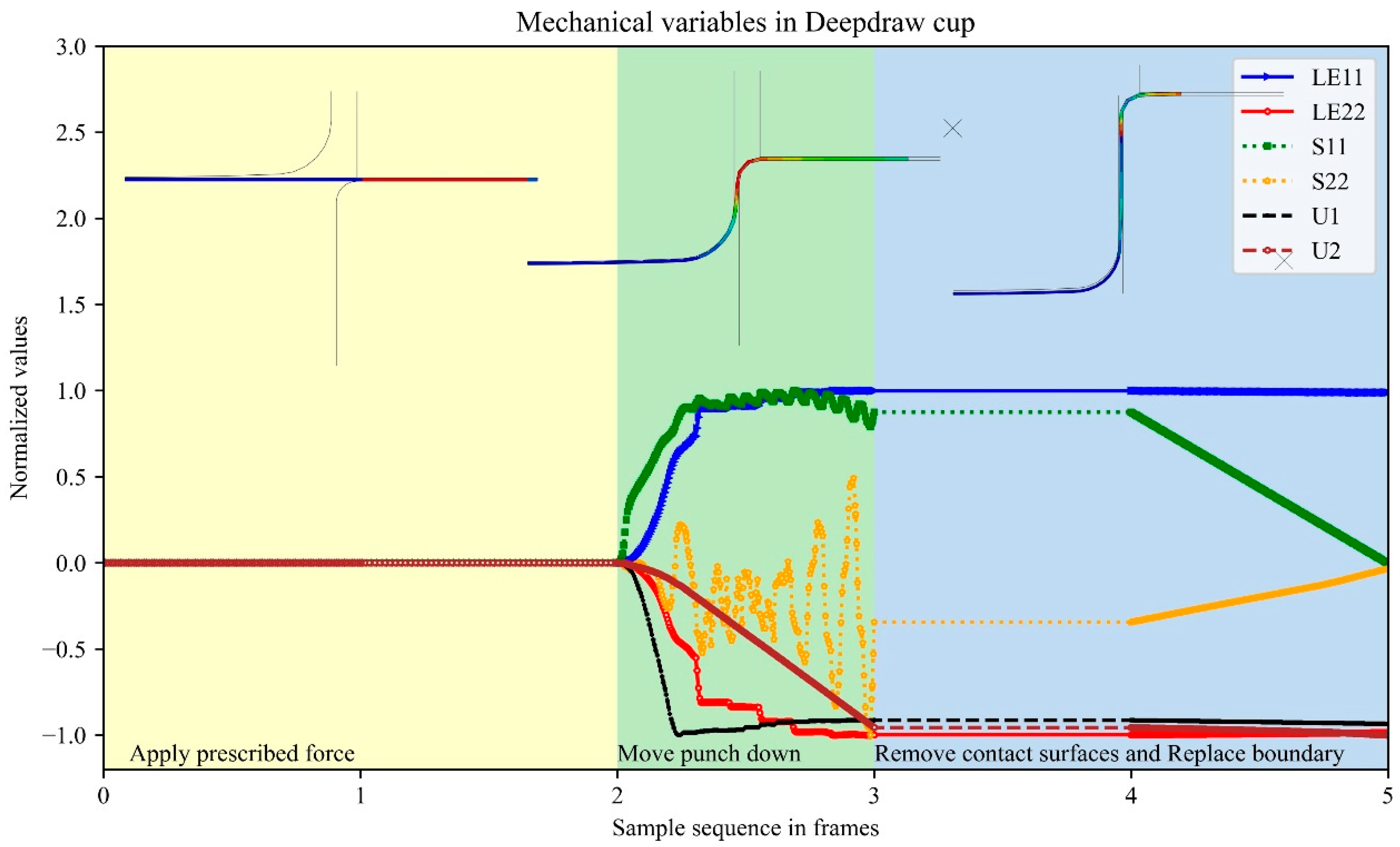
Figure A8.
Summary of causal relationships identified across the three stages of deepdraw cup.
References
- Ferrari, E.; Gargani, L.; Barbieri, G.; Ghiadoni, L.; Faita, F.; Bacciu, D. A causal learning framework for the analysis and interpretation of COVID-19 clinical data. PLoS ONE 2022, 17, e0268327. [Google Scholar] [CrossRef] [Scilit]
- Liu, J.; Xu, Y.; Wang, L. Fault information mining with causal network for railway transportation system. Reliab. Eng. Syst. Saf. 2022, 220, 108281. [Google Scholar] [CrossRef] [Scilit]
- Cheng, X.; Wu, P.; Liao, S.S.; Wang, X. An integrated model for crude oil forecasting: Causality assessment and technical efficiency. Energy Econ. 2023, 117, 106467. [Google Scholar] [CrossRef] [Scilit]
- Alyousef, M.I.; Sattar, M.U.; Hasan, R.; Usman, S.; Hassan, A. The Counterfactual–Dialectical Optimization Framework: A Prescriptive Approach to Employee Attrition Management with Empirical Validation. Information 2025, 16, 1053. [Google Scholar] [CrossRef] [Scilit]
- Altenbernd, A.; Wu, Z.; Kao, O. AmocRCA: At Most One Change Segmentation and Relative Correlation Ranking for Root Cause Analysis. In Proceedings of the 33rd ACM International Conference on the Foundations of Software Engineering, Trondheim, Norway, 23–28 June 2025; pp. 1386–1393. [Google Scholar] [CrossRef] [Scilit]
- Zang, H.; Li, M.; Jin, Z.; Huang, J. Unveiling construction accident causation: A scientometric analysis and qualitative review of research trends. Front. Built Environ. 2025, 11, 1602297. [Google Scholar] [CrossRef] [Scilit]
- Shrestha, A.; Giabbanelli, P.J. Are We Ready for Synchronous Conceptual Modeling in Augmented Reality? A Usability Study on Causal Maps with HoloLens 2. Information 2025, 16, 952. [Google Scholar] [CrossRef] [Scilit]
- Lin, T.; Song, K.; Jiang, Z.; Kang, Y.; Yuan, W.; Li, X.; Sun, C.; Huang, C.; Liu, X. Towards human-like perception: Learning structural causal model in heterogeneous graph. Inf. Process. Manag. 2024, 61, 103600. [Google Scholar] [CrossRef] [Scilit]
- Wu, X.; Zhong, Y.; Ling, Z.; Yang, J.; Li, L.; Sheng, W.; Jiang, B. Nonlinear learning method for local causal structures. Inf. Sci. 2024, 654, 119789. [Google Scholar] [CrossRef] [Scilit]
- Madhusoodanan, N.; Chiplunkar, R.; Puli, V.K.; Huang, B. Physics-informed sparse causal inference for source detection of plant-wide oscillations. J. Am. Inst. Chem. Eng. 2024, 70, e18362. [Google Scholar] [CrossRef] [Scilit]
- Zhou, S.; Cai, H.; Chen, H.; Ye, L. A Comparative Study of Causality Detection Methods in Root Cause Diagnosis: From Industrial Processes to Brain Networks. Sensors 2024, 24, 4908. [Google Scholar] [CrossRef] [Scilit]
- Wen, Y.; Huang, J.; Guo, S.; Elyahu, Y.; Monsonego, A.; Zhang, H.; Ding, Y.; Zhu, H. Applying causal discovery to single-cell analyses using CausalCell. eLife 2023, 12, e81464. [Google Scholar] [CrossRef] [Scilit]
- Zheng, S.; Wang, C.; Zio, E.; Liu, J. Fault detection in complex mechatronic systems by a hierarchical graph convolution attention network based on causal paths. Reliab. Eng. Syst. Saf. 2024, 243, 109872. [Google Scholar] [CrossRef] [Scilit]
- Gunjal, R.; Nayyer, S.S.; Wagh, S.R.; Stankovic, A.M.; Singh, N.M. Granger Causality for prediction in Dynamic Mode Decomposition: Application to power systems. Electr. Power Syst. Res. 2023, 225, 109865. [Google Scholar] [CrossRef] [Scilit]
- Yu, F.; Xiong, Q.; Cao, L.; Yang, F. Stable soft sensor modeling based on causality analysis. Control Eng. Pract. 2022, 122, 105109. [Google Scholar] [CrossRef] [Scilit]
- Waghen, K.; Ouali, M.-S. Multi-level interpretable logic tree analysis: A data-driven approach for hierarchical causality analysis. Expert Syst. Appl. 2021, 178, 115035. [Google Scholar] [CrossRef] [Scilit]
- Chen, S.; Jin, G.; Ma, X. Satellite On-Orbit Anomaly Detection Method Based on a Dynamic Threshold and Causality Pruning. IEEE Access 2021, 9, 86751–86758. [Google Scholar] [CrossRef] [Scilit]
- Li, S.; Pu, Z.; Cui, Z.; Lee, S.; Guo, X.; Ngoduy, D. Inferring heterogeneous treatment effects of crashes on highway traffic: A doubly robust causal machine learning approach. Transp. Res. Part C Emerg. Technol. 2024, 160, 104537. [Google Scholar] [CrossRef] [Scilit]
- Heyn, H.-M.; Mao, Y.; Weiss, R.; Knauss, E. Causal Models in Requirement Specifications for Machine Learning: A vision. In Proceedings of the 33rd ACM International Conference on the Foundations of Software Engineering, Trondheim, Norway, 23–28 June 2025; pp. 1402–1405. [Google Scholar] [CrossRef] [Scilit]
- Jia, S.; Li, Y.; Wang, X.; Sun, D.; Deng, Z. Deep causal factorization network: A novel domain generalization method for cross-machine bearing fault diagnosis. Mech. Syst. Signal Process. 2023, 192, 110228. [Google Scholar] [CrossRef] [Scilit]
- He, P.; Sun, R. Trend Analysis of Civil Aviation Incidents Based on Causal Inference and Statistical Inference. Aerospace 2023, 10, 822. [Google Scholar] [CrossRef] [Scilit]
- Liu, S.; Chen, S.; Wang, W.; Zhou, Z. Experimental and analytical study of grade Q690 high-strength steel square hollow section T joints under axial tension and compression. Structures 2024, 64, 106486. [Google Scholar] [CrossRef] [Scilit]
- Liu, J.; Böl, M. Experimental characterisation of the mechanical failure behaviour of whey protein gel treated with sodium hydroxide. Food Bioprod. Process. 2021, 129, 94–104. [Google Scholar] [CrossRef] [Scilit]
- Zniker, H.; Feddal, I.; El Kouifat, M.K.; El Magri, A.; El Hasnaoui, M. Numerical and experimental investigation of quasi-static indentation response of PVC foam sandwich and GFRP laminated composites. Int. Rev. Appl. Sci. Eng. 2025, 16, 11–21. [Google Scholar] [CrossRef] [Scilit]
- Lachambre, J.; Sibellas, A.; Adrien, J.; Papillon, J.; Bruant, R.; Maurel, G.; Maire, E. Experimental method for rubber deformation analysis using in situ X-ray tomography and digital volume correlation with FEM validation. Tomogr. Mater. Struct. 2025, 7, 100045. [Google Scholar] [CrossRef] [Scilit]
- Zhao, C.; Goh, K.L.; Lee, H.P.; Yin, C.; Zhang, K.; Zhong, J. Experimental study and finite element analysis on energy absorption of carbon fiber reinforced composite auxetic structures filled with aluminum foam. Compos. Struct. 2023, 303, 116319. [Google Scholar] [CrossRef] [Scilit]
- Zhang, B.; Zhang, X.; Wu, S.; Zhang, H. Indentation of expanded polystyrene foams with a ball. Int. J. Mech. Sci. 2019, 161–162, 105030. [Google Scholar] [CrossRef] [Scilit]
- Takalkar, A.S.; Chinnapandi, L.B.M. Multi-stage deep drawing process of axis-symmetric extra deep drawing steel cylindrical cup. Eng. Res. Express 2020, 2, 025008. [Google Scholar] [CrossRef] [Scilit]
- Coër, J.; Laurent, H.; Oliveira, M.C.; Manach, P.-Y.; Menezes, L.F. Detailed experimental and numerical analysis of a cylindrical cup deep drawing: Pros and cons of using solid-shell elements. Int. J. Mater. Form. 2018, 11, 357–373. [Google Scholar] [CrossRef] [Scilit]
- Chen, K.; Carter, A.J.; Korkolis, Y.P. Flange Wrinkling in Deep-Drawing: Experiments, Simulations and a Reduced-Order Model. J. Manuf. Mater. Process. 2022, 6, 76. [Google Scholar] [CrossRef] [Scilit]
- Kitson, N.K.; Constantinou, A.C.; Guo, Z.; Liu, Y.; Chobtham, K. A survey of Bayesian Network structure learning. Artif. Intell. Rev. 2023, 56, 8721–8814. [Google Scholar] [CrossRef] [Scilit]
- Constantinou, A.C.; Liu, Y.; Chobtham, K.; Guo, Z.; Kitson, N.K. Large-scale empirical validation of Bayesian Network structure learning algorithms with noisy data. Int. J. Approx. Reason. 2021, 131, 151–188. [Google Scholar] [CrossRef] [Scilit]
- Rosoł, M.; Młyńczak, M.; Cybulski, G. Granger causality test with nonlinear neural-network-based methods: Python package and simulation study. Comput. Methods Programs Biomed. 2022, 216, 106669. [Google Scholar] [CrossRef] [Scilit]
- La Bastide-van Gemert, S.; Stolk, R.P.; Van Den Heuvel, E.R.; Fidler, V. Causal inference algorithms can be useful in life course epidemiology. J. Clin. Epidemiol. 2014, 67, 190–198. [Google Scholar] [CrossRef] [Scilit]
- Ganopoulou, M.; Kangelidis, I.; Sianos, G.; Angelis, L. Causal Models for the Result of Percutaneous Coronary Intervention in Coronary Chronic Total Occlusions. Appl. Sci. 2021, 11, 9258. [Google Scholar] [CrossRef] [Scilit]
- Ramsey, J.; Spirtes, P.; Zhang, J. Adjacency-Faithfulness and Conservative Causal Inference. arXiv 2012, arXiv:1206.6843. [Google Scholar] [CrossRef] [Scilit]
- Nazaret, A.; Blei, D. Extremely Greedy Equivalence Search. arXiv 2025, arXiv:2502.19551. [Google Scholar] [CrossRef] [Scilit]
- Rathnam, C.; Lee, S.; Jiang, X. An algorithm for direct causal learning of influences on patient outcomes. Artif. Intell. Med. 2017, 75, 1–15. [Google Scholar] [CrossRef] [Scilit] [PubMed]
- Constantinou, A.C.; Liu, Y.; Kitson, N.K.; Chobtham, K.; Guo, Z. Effective and efficient structure learning with pruning and model averaging strategies. arXiv 2022, arXiv:2112.00398. [Google Scholar] [CrossRef] [Scilit]

Disclaimer/Publisher’s Note: The statements, opinions and data contained in all publications are solely those of the individual author(s) and contributor(s) and not of MDPI and/or the editor(s). MDPI and/or the editor(s) disclaim responsibility for any injury to people or property resulting from any ideas, methods, instructions or products referred to in the content. |
© 2026 by the author. Licensee MDPI, Basel, Switzerland. This article is an open access article distributed under the terms and conditions of the Creative Commons Attribution (CC BY) license.