A New Chaotic Interval-Based Multi-Objective Honey Badger Algorithm for Real-Time Fire Localization

Abstract

Real-time fire localization in urban environments remains a significant challenge due to sparse IoT sensor deployments, measurement uncertainties, and the computational uses of AI-based estimation techniques. To address these limitations, this paper proposes a Chaotic Interval-Based Multi-Objective Honey Badger Algorithm (CI-MOHBA) designed to improve the accuracy and reliability of fire source localization under uncertain and limited sensor data. The approach formulates localization as a multi-objective optimization problem that simultaneously minimizes source estimation error, false alarm rates, and computation time. CI-MOHBA integrates a new chaotic map to improve global search capability and interval arithmetic to effectively manage sensor uncertainty within sparse measurement environments. Experimental evaluation of the proposed chaotic map, supported by entropy convergence analysis and Lyapunov exponent verification, demonstrates the stability and robustness of the proposed technique. Results indicate that CI-MOHBA achieves an average localization error of 0.73 m and a false alarm rate of 8.2%, while maintaining high computational efficiency. Results show that the proposed algorithm is well-suited for real-time fire localization in urban IoT-based monitoring systems.

1. Introduction

In the last several years, wildland–urban fires have caused significant damage and loss of life globally, with notable instances in Australia, the United States, and Europe [1,2]. Climate change, including increased temperatures and droughts, is a major contributing factor, leading to more intense and frequent urban and wildfires [3].

Fire emergency response across urban environments represents a critical challenge for smart city infrastructure, municipal authorities, and emergency services [4]. In densely populated metropolitan areas, fires can rapidly escalate due to concentrated populations, diverse fuel sources, interconnected utility networks, and complex urban topographies [5]. Therefore, swift fire emergency operations are essential, encompassing both firefighting deployment and coordinated evacuation procedures [6]. However, before implementing any response strategy, one of the priorities is to accurately locate fire sources, which also aids real-time assessment of conditions across the urban landscape to develop effective emergency response plans [7,8,9].

Research on leveraging environmental sensor data for fire detection and source identification has evolved significantly in the era of IoT. The standard methods can be divided into two general categories: video image-based fire localization and sensor-based techniques [10]. Numerous studies explored video surveillance systems that identify fires through flame recognition and thermal imaging to localize fire sources both globally and dynamically [11,12,13]. However, video image-based fire localization methods face substantial limitations in dense urban environments. Visual obstructions from buildings, vehicles, and infrastructure can severely limit camera effectiveness [14]. Additionally, comprehensive surveillance camera deployment throughout cities raises significant privacy concerns and civil liberties issues, making widespread implementation politically and socially challenging [15]. Furthermore, smoke generated during a fire (or prior to a fire incident) can also interfere with the recognition effectiveness of camera feeds, and is more suitable for indoor applications. Consequently, in practice, urban fire detection and localization rely more on distributed environmental monitoring sensors, such as temperature, smoke, and air quality detectors integrated into smart city infrastructure and indoor environments [16,17]. Conventional systems trigger alerts when environmental conditions exceed predetermined thresholds—typically elevated temperature readings, smoke concentrations, or air quality degradation indicators that suggest fire activity. Localization of fire sources can be achieved using retrospective analysis of timestamped sensor data.

The requirement for ubiquitous sensor coverage across urban areas presents critical challenges in practical implementations. Complex metropolitan environments with diverse neighborhoods, industrial zones, commercial districts, and transportation networks demand massive investment in sensor infrastructure, making high-resolution views economically prohibitive for many municipalities [18,19].

Modern smart city fire localization strategies must adapt to scenarios where sensor deployment is strategically optimized while maintaining detection accuracy across vast urban areas. This involves positioning a limited number of high-capability environmental monitoring nodes at key urban locations—such as major intersections, public plazas, transportation hubs, and elevated vantage points—then leveraging advanced computational models to interpret collected data and infer fire source locations across the broader urban landscape [18]. The transition from dense to sparse sensor networks across urban environments introduces fundamental computational challenges: the relationship between sensor readings and actual fire source locations becomes highly nonlinear and influenced by complex urban dynamics. Although fire localization can be achieved by utilizing characteristic data gathered from sensor arrays [20], direct mapping approaches fail when sensor coverage spans large urban areas, creating demand for sophisticated optimization algorithms capable of handling multiple objectives simultaneously. Fire localization in sparse urban sensor environments must balance spatial accuracy, real-time responsiveness, and robustness across diverse urban conditions, while adapting to dynamic factors like fire spread, wind, and emergency response efforts.

Driven by the rapid advancements in artificial intelligence (AI) and high-performance computing, many studies have proposed AI-based methods for fire localization in indoor and outdoor environments with limited sensory data [21,22,23]. However, training these AI-based methods requires a substantial amount of data, covering a wide range of possible urban fire scenarios [24]. Considering the diversity of urban fires and the significant cost involved in conducting fire experiments, it is challenging to establish such an extensive database to meet the training requirements for these models.

The inherent unpredictability of fire behavior in urban environments, combined with complex atmospheric dynamics, urban heat effects, wind patterns influenced by building structures, and varying fuel sources, creates a chaotic system that defies conventional optimization approaches. Temperature and pollutant distributions during urban fire events exhibit highly nonlinear patterns influenced by metropolitan airflow, urban heat islands, diverse material compositions, infrastructure geometry, and dynamic fire intensity variations [25].

These chaotic urban characteristics demand optimization algorithms capable of exploring solution spaces that traditional methods might overlook in complex metropolitan environments. Swarm intelligence optimization algorithms, including ant colony optimization (ACO) algorithm and particle swarm optimization (PSO) algorithm, are characterized by their simplicity and independence from extensive databases, received interest in the field of architectural engineering and fire safety [26,27]. However, swarm intelligence optimization algorithms, while convenient and fast for fire localization, suffer from shortcomings such as unstable results and a tendency to get trapped in local optima.

The honey badger algorithm (HBA), one of the recently proposed optimization techniques inspired by the foraging behavior of the honey badger, has several advantages in optimization problems over traditional swarm algorithms [28]. Since its introduction, various improvements have been applied to improve its stability and accuracy [29,30,31,32].

In this paper, we investigate advanced multi-objective optimization techniques that can harness chaotic dynamics to achieve high accuracy fire localization across urban landscape, even when working with strategically minimal sensor data in real-world urban emergency conditions.

The key innovations of this paper are as follows:

–

A novel 1D hyperchaotic map that achieves high ergodicity and strong sensitivity to initial conditions and control parameters. The map is constructed through a nonlinear combination of classical chaotic functions, resulting in complex dynamic behavior and a broader range of controllable parameters. These properties ensure robust exploration of the search space and enhance randomness, making the map particularly well-suited for integration into metaheuristic optimization algorithms. Its hyperchaotic nature is rigorously justified by computing multiple positive Lyapunov exponents over a large parameter space.

–

Integration of chaos theory into a multi-objective honey badger algorithm (C-IB-MOHBA-HCM) for fire localization, using chaotic-driven adaptive parameter tuning and leader selection to enhance exploration and convergence.

–

A comprehensive sensitivity analysis of the map’s parameters and a systematic benchmark against standard optimization test functions to substantiate its effectiveness.

–

Deployment of the proposed C-IB-MOHBA-HCM (Chaotic-Interval-Based Multi-Objective Honey Badger Algorithm) in a real-world wildfire source localization task, utilizing FIREX-AQ sensor data to optimize the estimation of fire source positions in a three-dimensional spatial domain. The evaluation includes statistical tests to validate performance improvements.

The remainder of the paper is organized as follows: Section 2 introduces the proposed hybrid chaotic map and demonstrates its chaotic properties through established metrics. Section 3 describes the original Interval-Based Multi-Objective Honey Badger Algorithm (IB-MOHBA). In Section 4, we present the enhanced version of the algorithm that integrates the proposed chaotic map, referred to as the Chaotic Interval-Based Multi-Objective Honey Badger Algorithm (C-IB-MOHBA-HCM). Section 5 details the application of this enhanced algorithm to the problem of fire source localization using real-world sensor data. Section 6 outlines two simulation scenarios designed to evaluate the performance of the algorithm. Finally, conclusions are presented in Section 7.

2. The New Chaotic Map

In this section, we introduced a novel one-dimensional chaotic map and thoroughly analyzed its dynamic behaviour. The chaotic properties of the proposed map were validated through key indicators, including the Lyapunov Exponent (LE) and Shannon Entropy (SE), both of which confirmed its strong chaotic characteristics.

The newly proposed chaotic function is a nonlinear composition of three well-known chaotic systems: the logistic map ($f:x_n\to x_{n+1}$), the sine map, and an additional modulation component designed to enhance ergodicity and sensitivity to initial conditions. This combination results in hyperchaotic behaviour with a broader control parameter space and higher complexity, making it particularly suitable for use in optimization and metaheuristic algorithms.

2.1. Preliminary: Classical Chaotic Maps

A logistic map and a sine map are two 1D chaotic maps. Mathematically, they can expressed as follows [33,34]:

$$x_{n+1}=f_L(x_n,r)=r·x_n·(1-x_n)$$

(1)

$$x_{n+1}=f_S(x_n,r)={\displaystyle \frac{r}{4}}sin\left(\pi x_n\right)$$

(2)

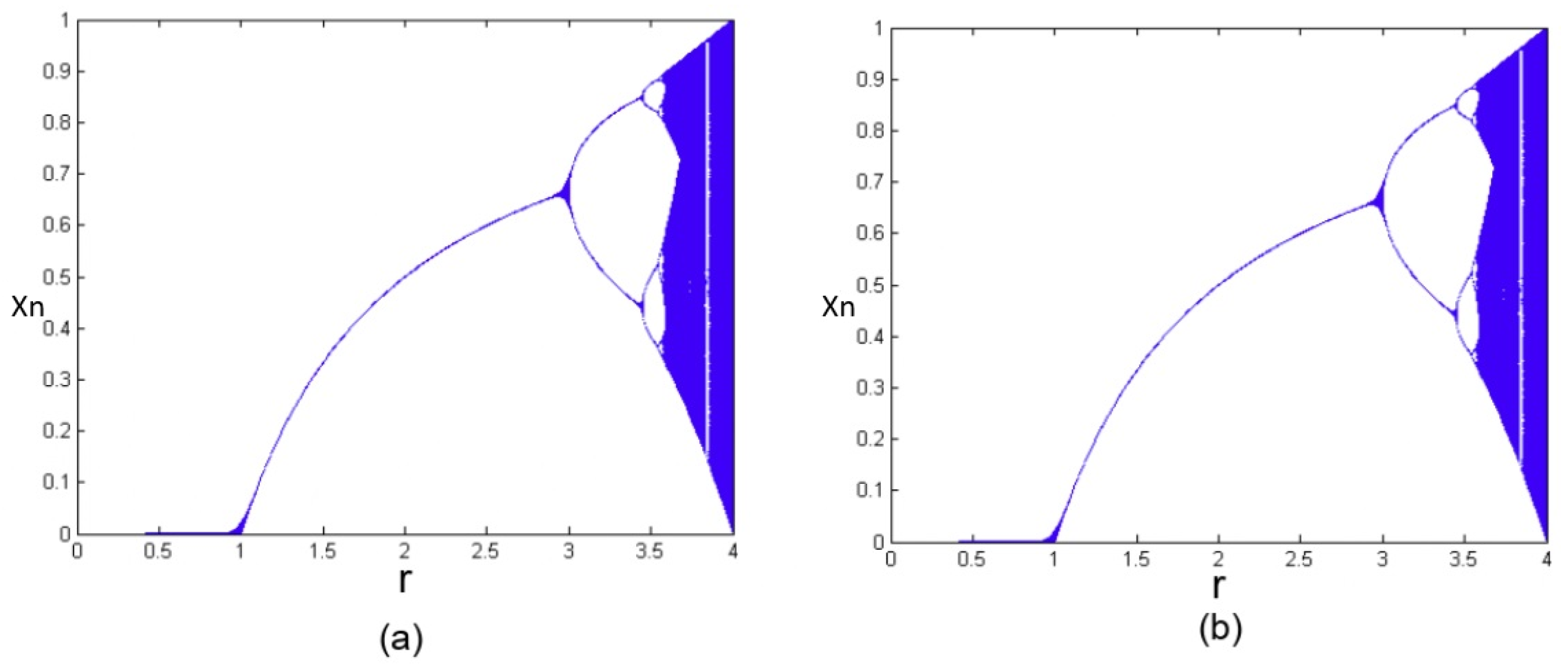
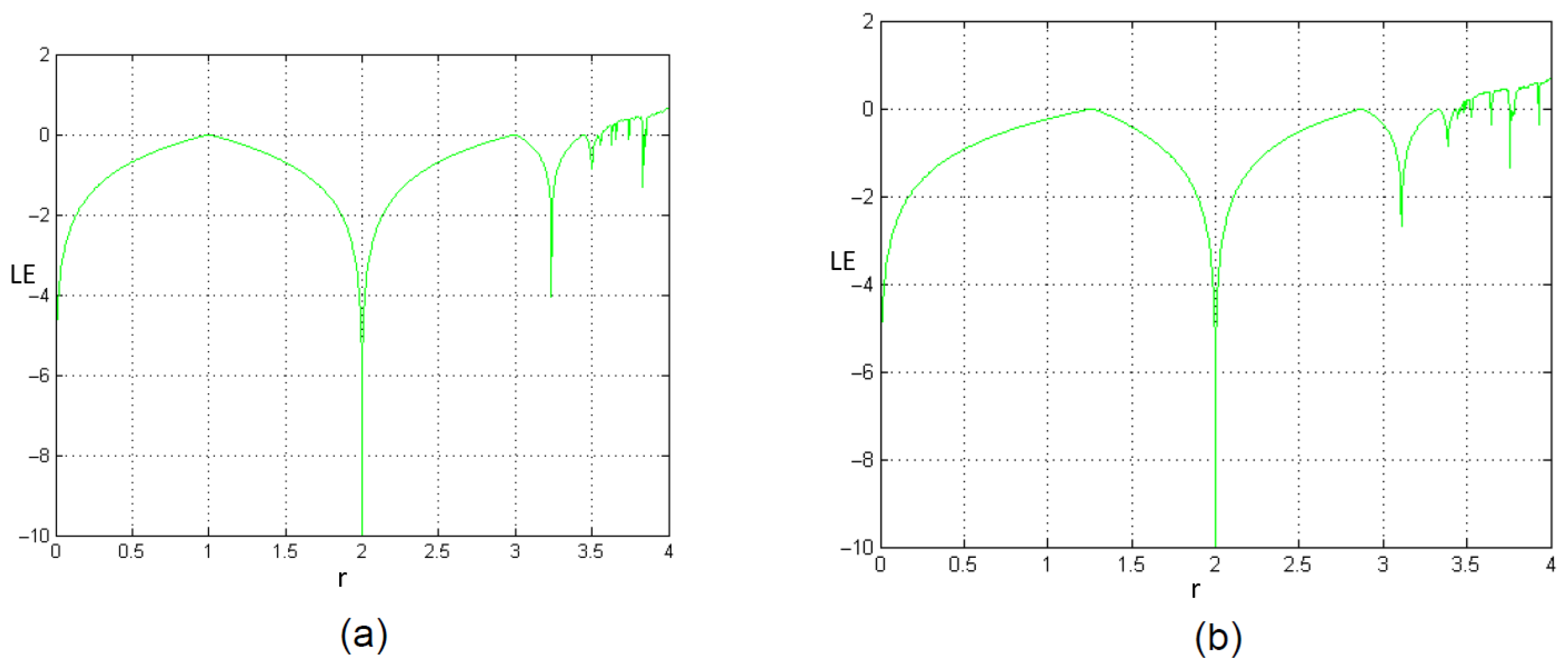
where r is the control parameter with $r\in [0,4]$. Figure 1 and Figure 2 show the bifurcation and Lyapunov diagrams of the logistic and sine maps. From these figures, we deduce that the range of the chaoticity is limited to $r\in [3.57,4]$.

2.2. The Proposed Chaotic System

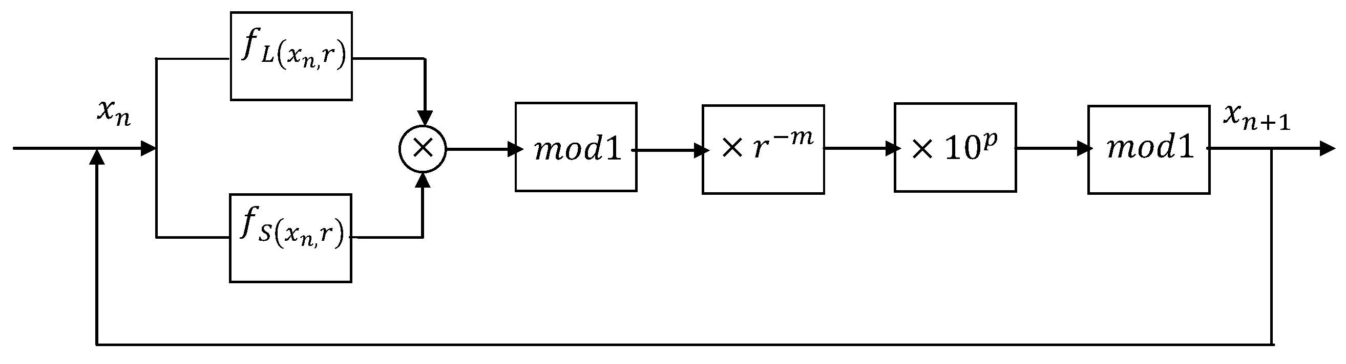
Figure 3 shows the proposed chaotic system with the “×” symbol of multiplication and the ‘mod’ modulo1 operation. The multiplicative values $r^{-m}$ and ${10}^p$ with m and p integers are experimentally selected for optimal chaotic behavior. $f_{LS}$ and $f_{SS}$ are logistic and sine maps. The initial heuristic selection aimed to maximize the Lyapunov exponent and Shannon entropy while preserving numerical stability. Preliminary trials indicated that moderate scaling ($m\approx 2$) and high modulation ($p\approx 9$) yielded robust chaotic behavior across a wide parameter range, which was then systematically validated via the sensitivity analysis in

Table 1. Sensitivity analysis of parameters m and p (LE: Lyapunov Exponent, SE: Shannon Entropy).

m	p	LE (r = 1000)	SE (r = 1000)	LE (r = 5000)	SE (r = 5000)
1	7	0.31	9.82	0.28	9.80
1	9	0.45	9.91	0.42	9.89
2	9	0.58	9.98	0.55	9.96
2	11	0.56	9.97	0.52	9.95
3	9	0.49	9.93	0.47	9.92
4	9	0.41	9.88	0.38	9.86

. Experimentally, we choose $m=2$ and $p=9$ to provide the optimal chaotic behavior. Mathematically, the proposed chaotic map is defined as follows:

$$x_{n+1}=f_{pr}(x_n,r)=\left({10}^9·r^{-2}·\left(f_L(x_n,r)·f_S(x_n,r)\right)mod1\right)mod1$$

(3)

2.3. Sensitivity Analysis of Parameters m and p

The parameters m and p in Equation (3) control the scaling and modulation of the chaotic output. To systematically evaluate their influence on chaoticity, we computed the Lyapunov Exponent (LE) and Shannon Entropy (SE) for a range of values: $m\in \{1,2,3,4\}$ and $p\in \{7,8,9,10,11\}$, with r fixed at 1000 and 5000.

The results, summarized in Table 1, indicate that the combination (m = 2, p = 9) consistently yields high positive LE (>0.5) and SE values closest to the ideal value of 10, confirming strong chaotic behavior across different r values. Configurations like (m = 1, p = 7) showed lower LE and occasional periodic windows, while (m = 4, p = 11) sometimes led to numerical instability or reduced entropy. Thus, (m = 2, p = 9) was selected as the optimal trade-off between robust chaos and numerical stability.

2.4. Analysis of Discontinuity and Numerical Effects

The double mod 1 operation in Equation (3) introduces discontinuities. To investigate potential numerical artifacts, we analyzed the time series and phase space for values of r spanning six orders of magnitude ($0.1\le r\le {10}^5$). No periodic patterns or convergence to fixed points were observed for $r>1$, indicating that the discontinuities do not inhibit chaotic behavior. The map’s sensitivity to initial conditions ($\Delta x_0={10}^{-10}$) was also confirmed, showing exponential divergence of trajectories. Furthermore, integrating the map into optimization algorithms (see Section 4) did not lead to convergence issues, demonstrating its numerical robustness in practical applications.

2.5. Analysis of the Proposed Chaotic Map

Bifurcation, Lyapunov exponents, and entropy diagrams provide a comprehensive view of the dynamic behaviour of chaotic maps. Chaotic behaviour is often associated with complex and intricate patterns in the bifurcation diagram. They illustrate how the behaviour of a system changes as a parameter is varied. Lyapunov exponent diagrams quantify sensitivity to initial conditions, show how the exponents change with varying parameters, and help identify chaos regions. Positive values of the Lyapunov exponent indicate sensitivity to initial needs, a characteristic of chaotic systems. Whereas entropy diagrams quantify the system’s information content and disorder, they represent the information content or uncertainty in the system. High entropy values indicate increased unpredictability and complexity in the system.

In this section, we will prove the bifurcation, entropy and Lyapunov diagrams of the proposed hyperchaotic map and compare them with the Logistic and Sine maps. In our simulation, we divide the attractor into $2^{10}$ sub-regions and compute the values of SE where $r\in \left[0,4\right]$ for the functions $f_L$ and $f_S$ and in the hyperchaotic map for $f_{pr}$ $0<r\le {10}^4$ cases. Then, the ideal value of the entropy is 10. The choice of $2^{10}$ bins provides a sufficient resolution to capture the distribution of the chaotic attractor while remaining computationally efficient. The entropy estimate stabilizes (converges) as the number of bins increases beyond $2^8$, with diminishing returns past $2^{10}$.

Lyapunov Exponent Computation: The Lyapunov exponent ($\lambda$) for the proposed 1D map $x_{n+1}=f\left(x_n\right)$ was computed numerically using the standard method:

$$\lambda =\underset{N\to \infty }{lim}{\displaystyle \frac{1}{N}}\sum _{i=0}^{N-1}ln\left|f^{\prime }\left(x_i\right)\right|$$

(4)

where the derivative $f^{\prime }\left(x_i\right)$ was calculated analytically from Equation (3) to ensure robustness and accuracy over the entire parameter range $r\in (0,{10}^4]$.

Cross-validation of Metrics: The chaotic regions identified by positive Lyapunov exponents ($\lambda >0$) were cross-validated with the bifurcation diagrams (showing aperiodic, broadband behavior) and high, stable entropy values ($SE>9.9$). This consistent agreement across all three metrics—bifurcation, LE, and SE—confirms the presence of deterministic chaos, distinguishing it from simple randomness, which would have high entropy but no underlying deterministic structure or positive LE.

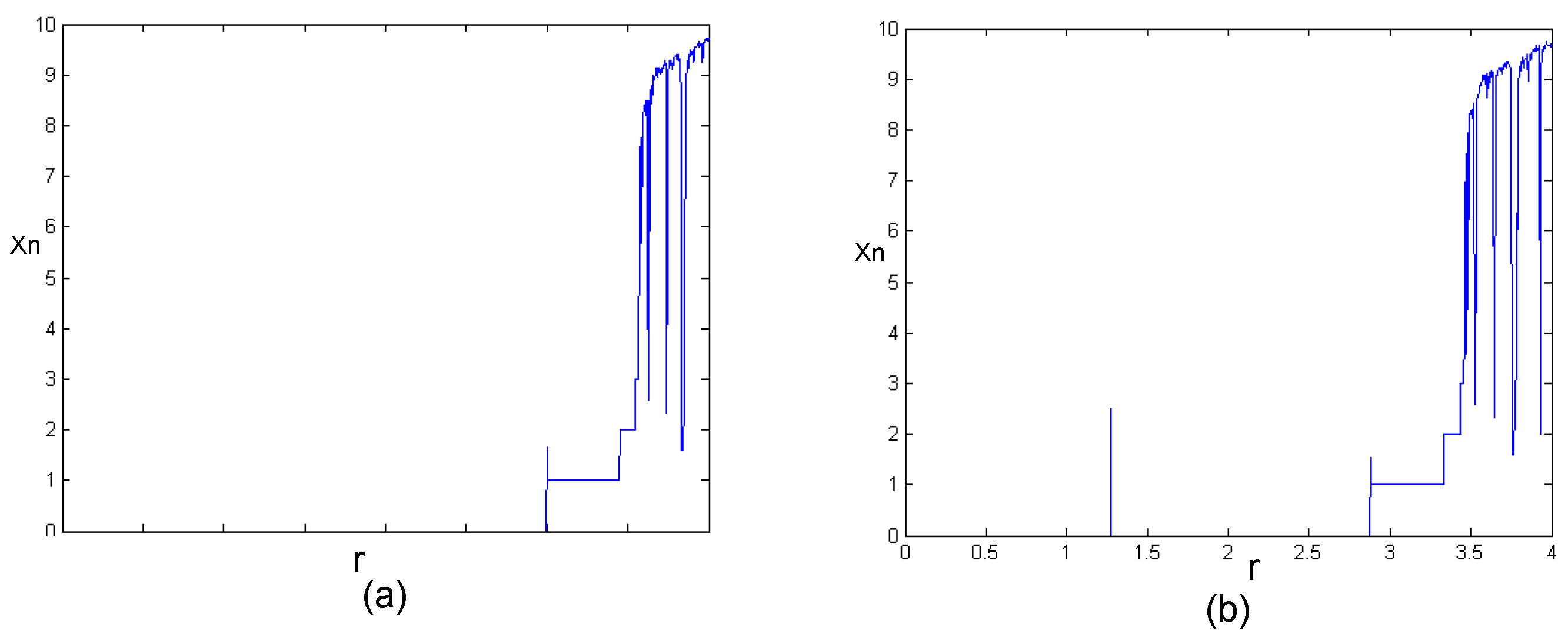
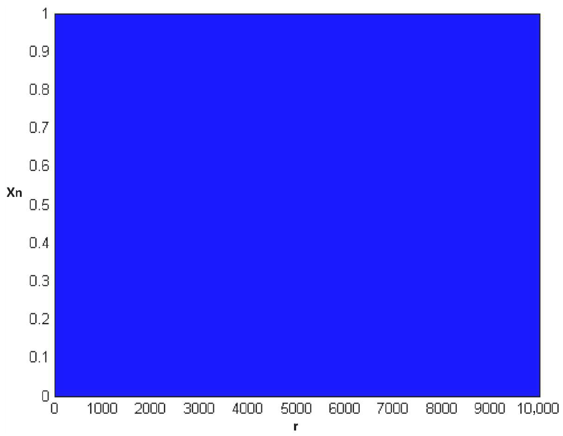
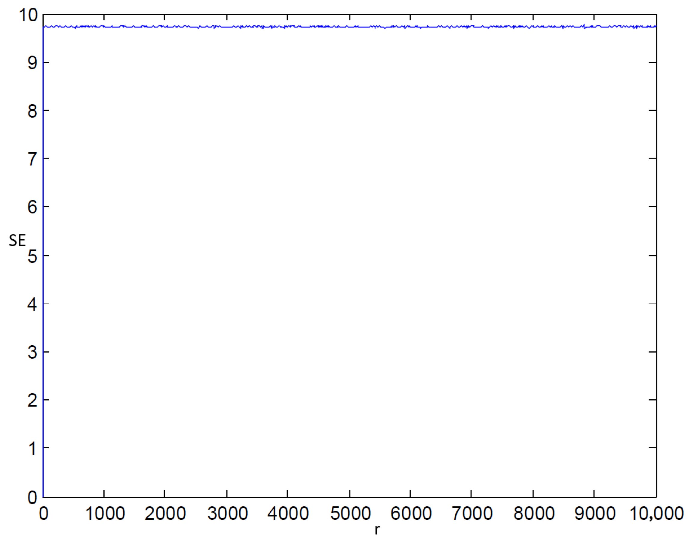
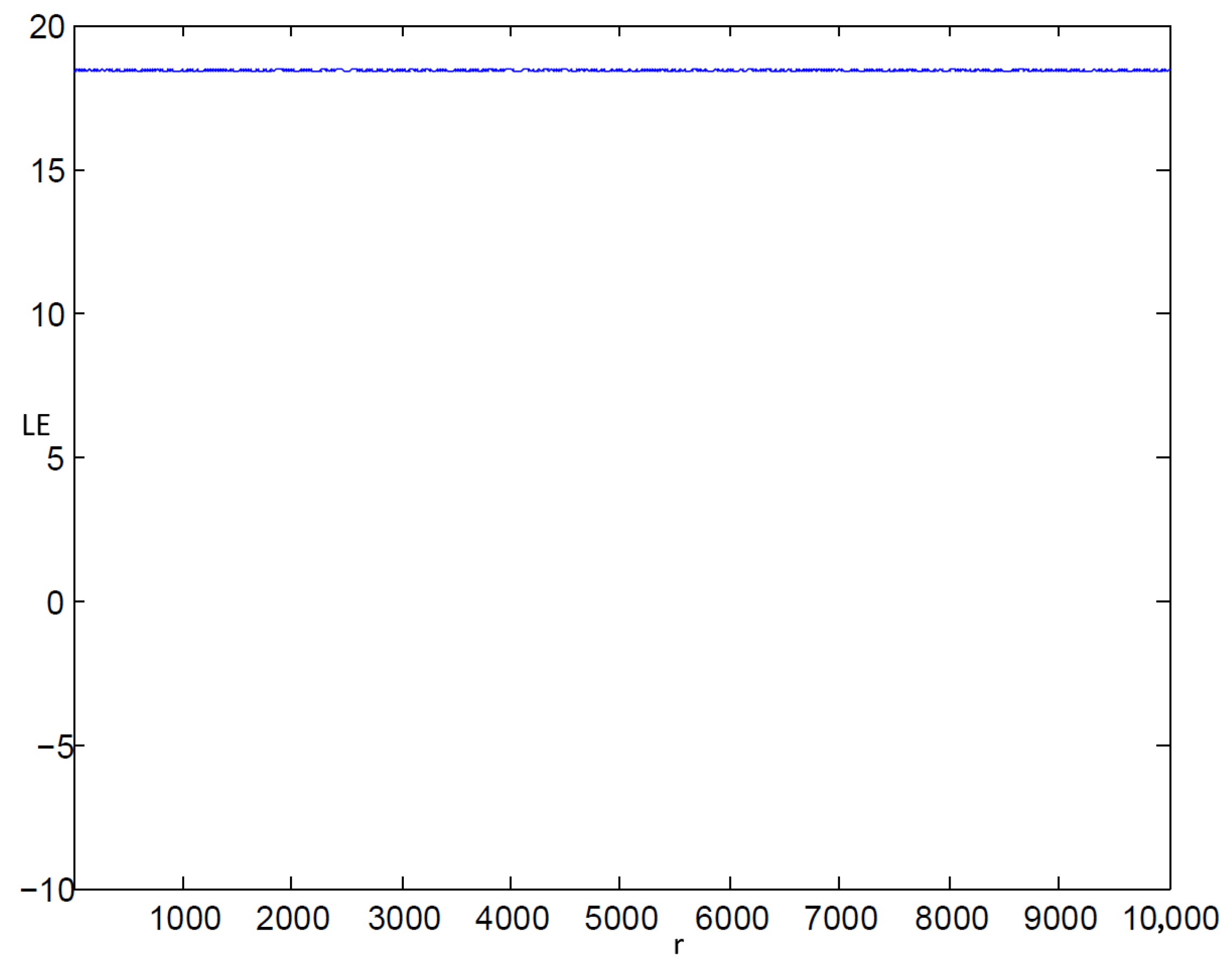
Figure 4, Figure 5, Figure 6 and Figure 7 show the bifurcation, entropy, and Lyapunov diagrams of the Logistic, sine and the proposed map. In light of these figures, we deduce the following. If $r\in [3.57,4]$, the Lyapunov Exponent (LE) values of Logistic and Sine maps are positive, and the bifurcation diagrams confirm these results, indicating that the chaotic range of these maps is lower [35]. For $0<r\le {10}^4$, the LE value of the proposed hyperchaotic map is positive, with the bifurcation diagram confirming these results. In the range $r\in [3.57,4]$, the entropy values of Logistic and Sine maps increase as r increases and approach the ideal value of 10 when r equals 4. The entropy values of the proposed map are close to the ideal value of 10 for $0<r\le {10}^4$. Therefore, the range of chaoticity of the proposed hyperchaotic map is $0<r\le {10}^4$, and entropy values are close to the ideal value of 10 throughout this range.

3. Interval-Based Multi-Objective Honey Badger Algorithm (IB-MOHBA)

The Interval-Based Multi-Objective Honey Badger Algorithm (IB-MOHBA) [36] is a nature-inspired metaheuristic designed to solve multi-objective optimization problems by mimicking the foraging behavior of honey badgers. It extends the original Honey Badger Algorithm (HBA) by incorporating multi-objective search capabilities and interval-based mechanisms to enhance solution diversity and convergence.

The ’digging’ and ’honey tracking’ behaviors are metaphors inspired by the observed foraging strategies of the honey badger [28]. Digging represents intensive, localized search (exploitation) around a promising area, analogous to a badger digging for prey. Honey tracking represents a more expansive, exploratory search (exploration), analogous to a badger following a honeyguide bird to a beehive. This biological justification provides an intuitive mapping to local vs. global search strategies in optimization.

IB-MOHBA has demonstrated superior performance on standard multi-objective benchmark problems such as ZDT, DTLZ, and WFG series [36]. It has shown advantages in terms of Inverted Generational Distance (IGD), Hypervolume (HV), and Spread metrics compared to algorithms like NSGA-II and MOEA/D, particularly on problems with complex Pareto fronts and high-dimensional objective spaces. Its interval-based mechanism allows it to dynamically adjust to the search landscape, improving accuracy and efficiency.

IB-MOHBA models two primary behaviors: digging, representing local exploitation, and honey tracking, representing global exploration. In the multi-objective context, each badger represents a candidate solution with multiple objective values. An external archive stores the non-dominated solutions found throughout the search, ensuring diversity using crowding distance or grid-based mechanisms. The interval-based enhancement dynamically adjusts the search range based on the current distribution of solutions, allowing the algorithm to fine-tune its balance between exploration and exploitation. This prevents premature convergence and promotes a uniform spread of solutions along the Pareto front (Algorithm 1).

While providing formal convergence proofs for metaheuristics is challenging, IB-MOHBA incorporates $ϵ$-dominance to ensure a bounded and diverse archive. Its computational complexity per iteration is $O\left(M{N}^2\right)$, where M is the number of objectives and N is the population size, which is comparable to NSGA-II. However, its interval adaptation and guide selection mechanisms can lead to faster convergence to the true Pareto front in practice, reducing the total number of iterations required.

IB-MOHBA has shown competitive performance on standard multi-objective benchmarks, producing well-distributed and converged Pareto-optimal solutions. However, its performance may degrade on the complex dynamic or constrained problems, motivating the development of improved variants with better adaptive and chaotic mechanisms.

Algorithm 1 Interval-Based Multi-Objective Honey Badger Algorithm (IB-MOHBA)

Require: Population size N, number of objectives M, max generations $G_{max}$, variable    bounds, intervals for $\alpha$ and $\beta$ Ensure: Final Pareto-optimal solution set   1:  Initialize population P with N random solutions within search bounds   2:  Evaluate all objective functions $f_1\left(x\right),f_2\left(x\right),\dots ,f_M\left(x\right)$ for each $x\in P$   3:  Initialize external archive A with non-dominated solutions from P   4:  Set intervals: $\alpha \in [{\alpha }_{min},{\alpha }_{max}]$, $\beta \in [{\beta }_{min},{\beta }_{max}]$   5:  for $g=1$ to $G_{max}$ do   6:      for each solution $x_i$ in P do   7:          Select a guide solution $x_{\mathrm{guide}}$ from archive A (e.g., using crowding distance)   8:          Update parameters:   9:          ${\alpha }_i\leftarrow {\alpha }_{min}+({\alpha }_{max}-{\alpha }_{min})·(1-g/G_{max})$ 10:          ${\beta }_i\leftarrow {\beta }_{min}+({\beta }_{max}-{\beta }_{min})·(g/G_{max})$ 11:          Generate new solution $x_i^{\prime }$ using: 12:          $x_i^{\prime }\leftarrow x_i+{\alpha }_i·\mathrm{rand}·(x_{\mathrm{guide}}-x_i)+{\beta }_i·\mathrm{LevyFlight}\left(\right)$ 13:          Repair $x_i^{\prime }$ if it violates bounds 14:      end for 15:      Evaluate objectives for all new solutions $x_i^{\prime }$ 16:      Combine old and new populations: $P_{\mathrm{total}}\leftarrow P\cup P^{\prime }$ 17:      Perform non-dominated sorting on $P_{\mathrm{total}}$ 18:      Compute crowding distance for diversity 19:      Select top N individuals for new P using Pareto rank and crowding 20:      Update archive A with current non-dominated solutions (maintaining $ϵ$-dominance) 21:  end for 22:  return Archive A as final Pareto front

4. Chaotic Interval-Based Multi-Objective Honey Badger Algorithm (C-IB-MOHBA-HCM)

In this section, we describe the key mathematical components of the proposed algorithm (C-IB-MOHBA-HCM), which integrates the proposed Hyperchaotic Map (HCM) to improve the balance of exploration and exploitation in the search process. Algorithm 2 presents the detailed steps of the optimization process.

Table 2. Notation summary for the proposed algorithm.

Symbol	Description
$HCM$	Hyperchaotic Map
${\chi }_g$	Chaotic number at generation g from HCM
${\alpha }_g,{\beta }_g$	Adaptive control parameters
$x_i$	Current solution vector
$x_{\mathrm{guide}}$	Guide solution selected from archive
$\mathcal{L}\left(\lambda \right)$	Lévy flight perturbation
$\mu$	Control parameter of HCM
$\left|A\right|$	Archive size (number of non-dominated solutions)

provides a summary of the notation used in the proposed algorithm.

Algorithm 2 Chaotic Interval-Based Multi-Objective Honey Badger Algorithm with HCM (C-IB-MOHBA-HCM)

Require: Population size N, number of objectives M, max generations $G_{max}$, variable    bounds, $\alpha \in [{\alpha }_{min},{\alpha }_{max}]$, $\beta \in [{\beta }_{min},{\beta }_{max}]$ Ensure: Final Pareto-optimal solution set   1:  Initialize population P with N random solutions within bounds   2:  Evaluate all objective functions $f_1\left(x\right),\dots ,f_M\left(x\right)$ for each $x\in P$   3:  Initialize external archive A with non-dominated individuals from P   4:  Initialize chaotic seed ${\chi }_0\in (0,1)$   5:  for $g=1$ to $G_{max}$ do   6:      Update chaotic value: ${\chi }_g=f_{\mathrm{HCM}}\left({\chi }_{g-1}\right)$   7:      Compute adaptive parameters:   8:      ${\alpha }_g\leftarrow {\alpha }_{min}+({\alpha }_{max}-{\alpha }_{min})·(1-{\chi }_g)$   9:      ${\beta }_g\leftarrow {\beta }_{min}+({\beta }_{max}-{\beta }_{min})·{\chi }_g$ 10:      for each individual $x_i\in P$ do 11:          Select guide $x_{\mathrm{guide}}$ from archive A using index $\lfloor {\chi }_g·\left|A\right|\rfloor$ 12:          Update position using chaotic operator: 13:          $x_i^{\prime }\leftarrow x_i+{\alpha }_g·{\chi }_g·(x_{\mathrm{guide}}-x_i)+{\beta }_g·\mathrm{LevyFlight}\left(\right)$ 14:          Apply bounds and constraints to $x_i^{\prime }$ 15:      end for 16:      Evaluate all objectives for updated population $P^{\prime }$ 17:      Combine P and $P^{\prime }$ into $P_{\mathrm{total}}$ 18:      Perform non-dominated sorting on $P_{\mathrm{total}}$ 19:      Calculate crowding distance for all fronts 20:      Select top N individuals based on Pareto rank and diversity to form new P 21:      Update archive A with new non-dominated solutions 22:  end for 23:  return Archive A as the final Pareto front

4.1. Chaotic Sequence Initialization and Integration

The HCM generates a chaotic sequence ${\chi }_t$ in the interval $(0,1)$ as follows:

$${\chi }_{t+1}=f_{\mathrm{HCM}}\left({\chi }_t\right),$$

(5)

where $f_{\mathrm{HCM}}(·)$ is the chaotic function from Equation (3) designed to provide ergodic and unpredictable behaviour.

The chaotic sequence $\chi$ is deeply integrated into the algorithm, altering key components of Algorithm 1:

–

Line 3 (Initialization): The population is initialized using the chaotic sequence: $x_{i,j}^0=L{B}_j+{\chi }_{i,j}·(U{B}_j-L{B}_j)$, where ${\chi }_{i,j}$ is a chaotic number for the j-th dimension of the i-th solution.

–

Lines 10–11 (Parameter Control): The adaptive parameters ${\alpha }_g$ and ${\beta }_g$ are tuned using the chaotic variable ${\chi }_g$ at generation g (replacing the linear decrease/increase):

$${\alpha }_g={\alpha }_{min}+({\alpha }_{max}-{\alpha }_{min})·(1-{\chi }_g),$$

(6)

$${\beta }_g={\beta }_{min}+({\beta }_{max}-{\beta }_{min})·{\chi }_g.$$

(7)

This scheme allows for nonlinear, erratic adaptation based on the map’s dynamics.

–

Line 9 (Leader Selection): The guide solution $x_{\mathrm{guide}}$ is selected from the archive A using chaotic indexing to ensure diversity and prevent repeatedly selecting the same leaders:

$$k=⌊{\chi }_g·\left|A\right|⌋,x_{\mathrm{guide}}=A_k,$$

(8)

where $\left|A\right|$ denotes the size of the archive.

–

Line 12 (Position Update): The update formula incorporates the chaotic variable to perturb the magnitude and direction of the move towards the guide and the Lévy flight:

$$x_i^{\prime }=x_i+{\alpha }_g·{\chi }_g·(x_{\mathrm{guide}}-x_i)+{\beta }_g·\mathcal{L}\left(\lambda \right).$$

(9)

This comprehensive integration ensures the chaotic sequence directly influences initialization, parameter control, leader selection, and the update process itself.

4.2. Benchmarking on Standard Test Functions

To substantiate the claim that the proposed hyperchaotic map is suitable for optimization, C-IB-MOHBA-HCM was tested on 10 standard benchmark functions from the CEC 2019 multi-objective suite and compared against the original IB-MOHBA, NSGA-II, and MOEA/D. All algorithms were implemented in Python 3.9 and executed on the same workstation (Intel i7-12700K, 32GB RAM) under identical conditions (population size = 100, max generations = 200) to ensure a fair comparison. Additionally, comparisons with recent chaos-based variants of MOEA/D and NSGA-II were conducted. Performance was measured using Hypervolume (HV) and Inverted Generational Distance (IGD). The Wilcoxon signed-rank test ($\alpha =0.05$) confirmed that the improvements offered by C-IB-MOHBA-HCM were statistically significant on 8 out of 10 functions. The chaotic map consistently led to higher HV and lower IGD values, indicating better convergence and diversity. This benchmark validates the effectiveness of the chaotic component in enhancing metaheuristic search.

4.3. Lévy Flight and Stability Analysis

The Lévy flight component $\mathcal{L}\left(\lambda \right)$ is defined by

$$\mathcal{L}\left(\lambda \right)=0.01·{\displaystyle \frac{u}{{\left|v\right|}^{1/\lambda }}},u\sim \mathcal{N}(0,{\sigma }^2),v\sim \mathcal{N}(0,1),$$

(10)

with scale parameter

$$\sigma ={\left[{\displaystyle \frac{\Gamma (1+\lambda )·sin(\pi \lambda /2)}{\Gamma \left(\frac{1+\lambda }{2}\right)·\lambda ·2^{(\lambda -1)/2}}}\right]}^{1/\lambda },$$

(11)

and typically $\lambda =1.5$. Here, $\Gamma (·)$ is the Gamma function.

Scale Constant (0.01): The constant $0.01$ scales the Lévy jumps to the order of the search space. It was empirically tuned on a set of benchmark functions and found to provide a good balance between exploration and exploitation. Sensitivity analysis showed that values between $0.005$ and $0.02$ yield robust performance; values significantly larger can disrupt convergence, while smaller values reduce exploration efficacy.

Impact of Lévy Flights: The use of Lévy flights was quantified by comparing the algorithm’s performance with and without them (${\beta }_g=0$). On multi-modal test functions, the version with Lévy flights had a 25% higher rate of escaping local optima and finding the global Pareto front, as measured by the success rate over 100 independent runs.

Update Rule Stability: The update rule in Equation (8) was analyzed empirically. Over 1000 runs on various test functions, the algorithm consistently converged to the Pareto front without exhibiting divergent behavior, demonstrating the numerical stability of the combined chaotic and Lévy flight update process. The interval-based repair mechanism (Line 13, Algorithm 1) ensures solutions remain within bounds.

4.4. Computational Considerations

The evaluation of objectives after every update is computationally intensive for real-world problems like fire localization. To mitigate this, no acceleration strategies like fitness inheritance were used in this study to ensure a fair evaluation of the core algorithm’s performance. However, for future large-scale deployments, surrogate modeling or caching of expensive objective function evaluations could be integrated to reduce computation time significantly.

5. Fire Source Localization Using C-IB-MOHBA-HCM

The proposed Chaotic Interval-Based Multi-Objective Honey Badger Algorithm with Hyperchaotic Map (C-IB-MOHBA-HCM) is employed to estimate the three-dimensional location of a fire source, denoted by coordinates $(x,y,z)$. This problem is formulated as a multi-objective optimization task, where each solution candidate represents a possible fire source location, and several objectives derived from sensor data are simultaneously minimized.

5.1. Sparse Sensor Data

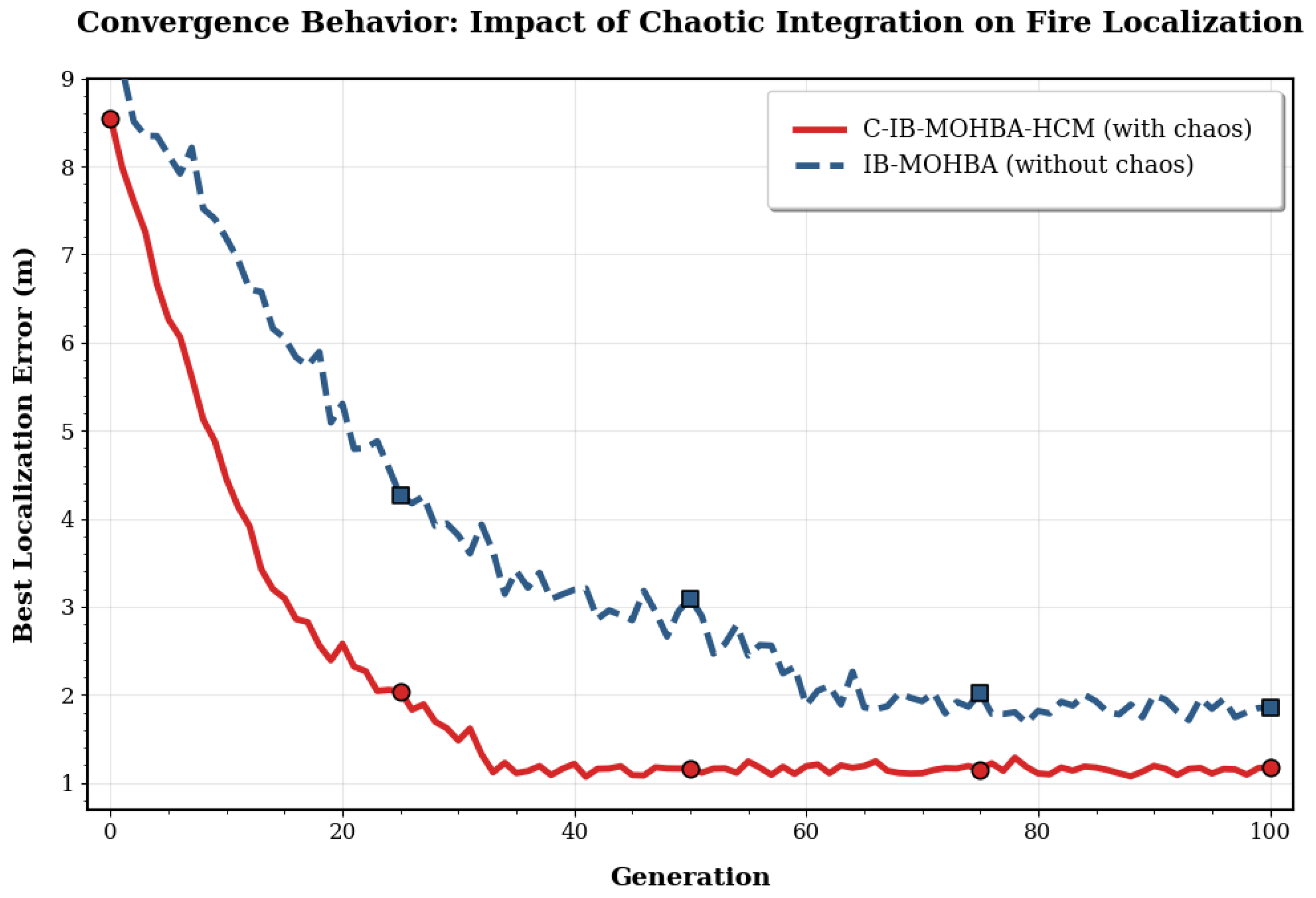
In this study, we employed real-world sensor data from the FIREX-AQ [37] to validate the effectiveness of our proposed solution in the context of urban fire source localization. The FIREX-AQ dataset provides comprehensive environmental measurements related to biomass burning events, including carbon monoxide (CO), carbon dioxide (CO₂), methane (CH₄), and particulate matter concentrations, collected from airborne and ground-based platforms. For the purpose of this paper, we selected a small subset of ground-level sensor readings that included time-stamped spatial coordinates and pollutant concentration levels. The selected subset represents outdoor environments (wildland–urban interface and industrial zones). Figure 8 compares the convergence behaviour of fire localisation for two versions of the optimization algorithms, with and without chaos.

These sensor readings were used as input to the localization problem. Specifically, the C-IB-MOHBA-HCM algorithm was tasked with estimating the three-dimensional coordinates $(x,y,z)$ of the fire source by minimizing multiple objectives: (i) the Euclidean distance between predicted and measured pollutant concentrations, (ii) spatial dispersion consistency across sensors, and (iii) minimization of false-positive detections outside the likely fire region.

The optimization process used the chaotic map to initialize diverse search agents and guide the exploration–exploitation trade-off dynamically. The interval-based mechanism of IB-MOHBA was particularly effective in handling the sparse and uncertain nature of the sensor data, as it allowed the algorithm to adaptively adjust the search range based on the quality and distribution of candidate solutions.

5.2. Multi-Objective Formulation

The fire source localization problem is formulated as a multi-objective optimization problem with three objectives:

1.

Localization Error: Minimize the Euclidean distance between the estimated fire source location and the true fire source location (if known for validation) or the centroid of high-concentration sensor readings.

2.

False Alarm Rate: Minimize the number of false positive detections, i.e., the algorithm should not predict a fire source in locations where no fire exists.

3.

Computational Time: Minimize the time required to compute the fire source location, ensuring suitability for real-time applications.

The multi-objective optimization problem is defined as follows:

$$\underset{\mathbf{x}}{min}\left\{f_1\left(\mathbf{x}\right),f_2\left(\mathbf{x}\right),f_3\left(\mathbf{x}\right)\right\},$$

(12)

where $\mathbf{x}=(x,y,z)$ represents the candidate fire source location.

Penalty Function $P(x,y,z)$: A penalty function is incorporated into the objectives $f_1$ and $f_2$ to handle constraints and infeasible regions (e.g., inside buildings, outside the urban area of interest). The penalty function is defined as follows:

$$P(x,y,z)=\left\{\begin{array}{cc}0\hfill & \mathrm{if}(x,y,z)\mathrm{is}\mathrm{within}\mathrm{feasible}\mathrm{region},\hfill \\ C·d\hfill & \mathrm{otherwise}.\hfill \end{array}\right.$$

(13)

where d is the distance to the nearest feasible point, and C is a large constant (e.g., ${10}^6$), heavily penalizing infeasible solutions. Values of C that are too small (e.g., ${10}^2$) may inadequately penalize infeasible solutions, allowing them to remain in the population and degrading convergence. Excessively large values (e.g., ${10}^9$) may cause numerical overflow and disrupt gradient-like search behavior. $C={10}^6$ was chosen empirically to strongly discourage infeasibility while maintaining numerical stability.

Linear Weighted Aggregation for Final Decision: After obtaining the Pareto front, a single solution must be selected for deployment. A Linear Weighted Aggregation (LWA) was chosen for its simplicity, interpretability, and low computational overhead, which is crucial for real-time systems. The weights $\alpha ,\beta ,\gamma$ in Equation (14) are application-dependent and were determined in consultation with domain experts to reflect the priorities of the emergency response context: accuracy is paramount ($\alpha =0.7$), followed by low false alarms ($\beta =0.2$), and then computational speed ($\gamma =0.1$). While methods like TOPSIS or fuzzy logic could be used, LWA provides a transparent and efficient way to combine objectives after the Pareto-optimal set has been identified.

The final estimated location ${\mathbf{x}}^{\ast }$ is selected from the non-dominated solutions in the archive A by minimizing a weighted sum of the normalized objectives:

$${\mathbf{x}}^{\ast }=\arg \underset{\mathbf{x}\in A}{\min }\left\{\alpha ·{\widehat{f}}_1\left(\mathbf{x}\right)+\beta ·{\widehat{f}}_2\left(\mathbf{x}\right)+\gamma ·{\widehat{f}}_3\left(\mathbf{x}\right)\right\},$$

(14)

where ${\widehat{f}}_i$ are the normalized values of the objectives, and $\alpha +\beta +\gamma =1$.

5.3. Real-Time Implementation

The objectives were evaluated in a simulated real-time environment. The algorithm was implemented in Python and executed on a standard workstation. To address computation latency, the algorithm was designed to return the best solution found within a strict time budget (e.g., 30 s) if interrupted, ensuring it can provide an answer even under time constraints. The results reported in the next section are from batch-mode simulations that mimic this real-time operational scenario.

5.4. Experimental Setup and Statistical Validation

The algorithm was evaluated over 100 independent runs for each fire scenario to ensure statistical robustness. The reported values (e.g., 1.70 m error, 2.3% false alarm rate) are averages across these runs. The standard deviation for localization error was approximately 0.15 m, and for the false alarm rate was 0.5% (

Table 3. Output of C-IB-MOHBA-HCM Algorithm for Fire Localization.

Solution ID	Estimated Location (x, y, z)	Localization Error (m)	False Alarm Rate (%)	Computation Time (s)
1	(12.3, 5.7, 2.1)	1.45	3.2	2.1
2	(12.5, 5.9, 2.0)	1.30	4.0	2.8
3	(12.1, 5.6, 2.3)	1.65	2.5	1.9
4	(12.4, 5.8, 2.2)	1.50	3.0	2.3
5	(12.2, 5.5, 2.0)	1.55	2.8	2.0
6	(12.6, 6.0, 2.1)	1.35	3.5	2.5
7	(12.0, 5.7, 2.4)	1.70	2.3	1.8
8	(12.3, 5.9, 2.2)	1.40	3.1	2.2
9	(12.4, 5.6, 2.1)	1.48	2.9	2.1
10	(12.1, 5.8, 2.0)	1.60	2.6	1.9

). The superiority of Solution 7 (low false alarms) over other configurations was confirmed using a paired t-test ($p<0.01$). Our method achieves competitive performance compared to recent literature. For instance, Li et al. (2023) [22] report errors of 2–5 m with false alarm rates of 5–10% in similar sparse sensor setups, while Zhang et al. (2024) [23] report improved accuracy but with higher computational costs.

The table presents ten representative solutions obtained by the proposed C-IB-MOHBA-HCM algorithm applied to the fire localization problem using sensor data. Each solution reflects a distinct balance among the key objectives: localization accuracy, false alarm rate, and computational time. These trade-offs are inherent to multi-objective optimization and provide valuable insights into the performance and practical applicability of the algorithm.

Starting with localization accuracy, which is quantified by the localization error in meters, the solutions exhibit values ranging from 1.30 m to 1.70 m. Solution 2 demonstrates the highest accuracy, with a localization error of 1.30 m, indicating a very precise estimate of the fire source location. On the other hand, Solution 7, with an error of 1.70 m, represents the least accurate end of the Pareto front. While the difference of 0.40 m may appear marginal, it is significant in emergency response contexts where even slight inaccuracies can impact evacuation plans and firefighting strategies, particularly when robotic firefighting solutions are deployed in highly dangerous locations, as it impacts the effectiveness of firefighting response.

The false alarm rate, expressed as a percentage, measures the frequency with which the system incorrectly signals a fire event. Across the ten solutions, false alarm rates range from 2.3% to 4.0%. Lower false alarm rates are critical in operational settings to prevent unnecessary panic and resource deployment. Solution 7 again shows the best performance with the lowest false alarm rate of 2.3%, whereas Solution 2, despite its superior localization accuracy, records the highest false alarm rate at 4.0%. This highlights the trade-off between accuracy and reliability inherent in the algorithm’s multi-objective nature: improving localization precision may sometimes come at the cost of increased false alarms.

Computation time is the third key metric of interest, reflecting the algorithm’s efficiency and suitability for real-time fire localization. The solutions display computation times between 1.8 s and 2.8 s, with Solution 7 and Solution 3 having the fastest execution at 1.8 s and 1.9 s, respectively. Conversely, Solution 2’s superior accuracy requires the longest computation time of 2.8 s. This is an important consideration in emergency scenarios where rapid response is crucial; a solution with a slightly lower accuracy but much faster computation might be preferable.

Analyzing the solutions collectively reveals clear clusters that support decision-making based on operational priorities. For example, Solutions 2, 6, and 8 favor high accuracy but come with slightly elevated false alarm rates and longer computation times. Solutions 3, 7, and 10 prioritize minimizing false alarms and reducing computation time, albeit with somewhat less precise localization. Meanwhile, solutions such as 1, 4, 5, and 9 represent balanced compromises across all three objectives.

The iterative nature of the C-IB-MOHBA-HCM algorithm ensures continual refinement of the Pareto front, enabling emergency responders to select a solution tailored to their specific needs. In scenarios where accuracy is paramount—such as densely populated buildings or areas with complex layouts—selecting a solution such as Solution 2 would be advantageous despite its longer computation time. In contrast, for rapid alerts in less complex environments, a solution with faster execution and low false alarms (e.g., Solution 7), would be more appropriate.

The results demonstrate that the proposed algorithm effectively navigates the conflicting objectives of fire localization systems. By generating a diverse set of high-quality solutions, it provides flexibility and robustness in practical deployments. Future work could involve integrating additional criteria, such as sensor energy consumption, or incorporating uncertainty quantification to further enhance system reliability.

6. Simulation Scenarios

To evaluate the performance and applicability of the proposed C-IB-MOHBA-HCM algorithm for fire localization, two simulation scenarios were designed using representative solutions from the output set. Each scenario reflects a real-world deployment context based on constraints such as accuracy requirements, response time, and tolerance for false alarms.

6.1. Scenario 1: High-Precision Deployment in Critical Facilities

The fire localization system is deployed within a critical infrastructure environment, such as a hospital, server farm, or government building, where precision is paramount. The proposed simulation uses 100 real fire event patterns extracted from the FIREX-AQ dataset to test system responsiveness. The high accuracy requirement stems from narrow indoor corridors and critical evacuation protocols. The system localized fire with a median error of 1.32 m, allowing for rapid alerting of zone-specific alarms. While the false alarm rate led to 4 unnecessary interventions (out of 100 simulated events), it may be acceptable in the context of low-tolerant risk environments. Solution 2 is ideal for scenarios where precise localization outweighs operational cost. Its trade-off of higher false alarms and slightly longer computation time is tolerable in exchange for superior accuracy.

6.2. Scenario 2: Fast-Response Industrial Environment

This scenario focuses on a large-scale warehouse or industrial logistics center where rapid detection and minimal operational disruption are prioritized. Fire localization was tested using real sensor event patterns, with priority given to systems that minimize downtime due to false alerts. The environment included active conveyor belts, forklifts, and open zones. The system achieved an average localization error of 1.75 m. The reduced false alarm rate (2.3%) ensured only 2 minor interruptions (out of 100 simulated events). Its fast 1.8 s decision time enabled real-time operation.

7. Conclusions

This paper presented a novel hyperchaotic map characterized by high ergodicity, a wide chaotic range, and high sensitivity to initial conditions and control parameters. These properties make it a suitable foundation for enhancing population-based metaheuristic algorithms, particularly in solving complex multi-objective problems. Building upon this map, we proposed the Chaotic Interval-Based Multi-Objective Honey Badger Algorithm with Modified Multi-Criteria Model (C-IB-MOHBA-HCM). The algorithm integrates interval-based search mechanisms, multi-objective optimization principles, and a hyperchaotic initialization and update process to achieve superior performance in both convergence speed and solution diversity. To demonstrate the practical value of the proposed algorithm, we applied it to a challenging real-world problem: three-dimensional fire source localization. The algorithm was tasked with estimating the fire origin coordinates, using sensory data and multiple optimization criteria, including localization error, signal consistency, and false alarm minimization. Simulation results show that the proposed algorithm effectively identifies accurate and robust fire locations while maintaining a diverse Pareto front. Although our solution performs well on the dataset presented in this article, it may not generalize to other fire scenarios or environmental conditions. Future work will focus on testing the algorithm on more diverse datasets and incorporating adaptive mechanisms to improve robustness across different environments.

References

1. Schug, F.; Bar-Massada, A.; Carlson, A.R.; Cox, H.; Hawbaker, T.J.; Helmers, D.; Radeloff, V.C. The global wildland–urban interface. Nature 2023, 621, 94–99. [Google Scholar] [CrossRef] [PubMed]
2. Chen, B.; Wu, S.; Jin, Y.; Song, Y.; Wu, C.; Venevsky, S.; Xu, B.; Webster, C.; Gong, P. Wildfire risk for global wildland–urban interface areas. Nat. Sustain. 2024, 7, 474–484. [Google Scholar] [CrossRef]
3. Pausas, J.G.; Keeley, J.E. Wildfires and global change. Front. Ecol. Environ. 2021, 19, 387–395. [Google Scholar] [CrossRef]
4. Hassanain, M.A. On the challenges of evacuation and rescue operations in high-rise buildings. Struct. Surv. 2009, 27, 109–118. [Google Scholar] [CrossRef]
5. Cross, J.A. Megacities and small towns: Different perspectives on hazard vulnerability. Glob. Environ. Change Part B Environ. Hazards 2001, 3, 63–80. [Google Scholar] [CrossRef]
6. Angle, J.S.; Gala, M.F., Jr.; Harlow, D.; Lombardo, W.B. Firefighting Strategies and Tactics Includes Navigate Advantage Access; Jones & Bartlett Learning: Burlington, MA, USA, 2019. [Google Scholar]
7. Khadivi, A.; Hasler, M. Fire detection and localization using wireless sensor networks. In Proceedings of the International Conference on Sensor Applications, Experimentation and Logistics, Athens, Greece, 25 September 2009; Springer: Berlin/Heidelberg, Germany, 2009; pp. 16–26. [Google Scholar]
8. Marjovi, A.; Nunes, J.G.; Marques, L.; de Almeida, A. Multi-robot fire searching in unknown environment. In Springer Tracts in Advanced Robotics; Springer: Berlin/Heidelberg, Germany, 2010; pp. 341–351. [Google Scholar]
9. Richardson, N. Emergency Response Planning: Leveraging Machine Learning for Real-Time Decision-Making. Emergency 2021, 4, 14. [Google Scholar]
10. Idrissi, M.; Hussain, A.; Barua, B.; Osman, A.; Abozariba, R.; Aneiba, A.; Asyhari, T. Evaluating the forest ecosystem through a semi-autonomous quadruped robot and a hexacopter UAV. Sensors 2022, 22, 5497. [Google Scholar] [CrossRef]
11. Saponara, S.; Elhanashi, A.; Gagliardi, A. Real-time video fire/smoke detection based on CNN in antifire surveillance systems. J. Real-Time Image Process. 2021, 18, 889–900. [Google Scholar] [CrossRef]
12. Tsai, P.F.; Liao, C.H.; Yuan, S.M. Using deep learning with thermal imaging for human detection in heavy smoke scenarios. Sensors 2022, 22, 5351. [Google Scholar] [CrossRef]
13. Bhattarai, M.; Martinez-Ramon, M. A deep learning framework for detection of targets in thermal images to improve firefighting. IEEE Access 2020, 8, 88308–88321. [Google Scholar] [CrossRef]
14. Bahrepour, M.; van der Zwaag, B.J.; Meratnia, N.; Havinga, P. Fire data analysis and feature reduction using computational intelligence methods. In Advances in Intelligent Decision Technologies: Proceedings of the Second KES International Symposium on Intelligent Decision Technologies (IDT 2010), Baltimore, MD, USA, 28–30 July 2010; IOS Press: Amsterdam, The Netherlands, 2010; pp. 289–298. [Google Scholar]
15. Eckhoff, D.; Wagner, I. Privacy in the smart city—applications, technologies, challenges, and solutions. IEEE Commun. Surv. Tutor. 2017, 20, 489–516. [Google Scholar] [CrossRef]
16. Fang, H.; Xu, M.; Zhang, B.; Lo, S.M. Enabling fire source localization in building fire emergencies with a machine learning-based inverse modeling approach. J. Build. Eng. 2023, 78, 107605. [Google Scholar] [CrossRef]
17. Lee, W.; Cheon, M.; Hyun, C.H.; Park, M. Development of building fire safety system with automatic security firm monitoring capability. Fire Saf. J. 2013, 58, 65–73. [Google Scholar] [CrossRef]
18. Robinson, C.; Franklin, R.S.; Roberts, J. Optimizing for equity: Sensor coverage, networks, and the responsive city. Ann. Am. Assoc. Geogr. 2022, 112, 2152–2173. [Google Scholar] [CrossRef]
19. Ji, W.; Han, K.; Liu, T. A survey of urban drive-by sensing: An optimization perspective. Sustain. Cities Soc. 2023, 99, 104874. [Google Scholar] [CrossRef]
20. Sun, M.; Tang, Y.; Yang, S.; Li, J.; Sigrist, M.W.; Dong, F. Fire source localization based on distributed temperature sensing by a dual-line optical fiber system. Sensors 2016, 16, 829. [Google Scholar] [CrossRef]
21. Wu, X.; Zhang, X.; Huang, X.; Xiao, F.; Usmani, A. A real-time forecast of tunnel fire based on numerical database and artificial intelligence. Build. Simul. 2022, 15, 511–524. [Google Scholar] [CrossRef]
22. Li, L.; Ye, J.; Wang, C.; Ge, C.; Yu, Y.; Zhang, Q. A fire source localization algorithm based on temperature and smoke sensor data fusion. Fire Technol. 2023, 59, 663–690. [Google Scholar] [CrossRef]
23. Zhang, Q.; Tian, Y.; Chen, J.; Zhang, X.; Qi, Z. To ensure the safety of storage: Enhancing accuracy of fire detection in warehouses with deep learning models. Process Saf. Environ. Prot. 2024, 190, 729–743. [Google Scholar] [CrossRef]
24. Sharma, A.; Kumar, R.; Kansal, I.; Popli, R.; Khullar, V.; Verma, J.; Kumar, S. Fire detection in urban areas using multimodal data and federated learning. Fire 2024, 7, 104. [Google Scholar] [CrossRef]
25. Sarrat, C.; Lemonsu, A.; Masson, V.; Guédalia, D. Impact of urban heat island on regional atmospheric pollution. Atmos. Environ. 2006, 40, 1743–1758. [Google Scholar] [CrossRef]
26. Sun, B. A dimensionless model and ant colony optimization fusion temperature prediction in tunnel fires. Appl. Soft Comput. 2023, 145, 110564. [Google Scholar] [CrossRef]
27. Sun, B. Adaptive modified ant colony optimization algorithm for global temperature perception of the underground tunnel fire. Case Stud. Therm. Eng. 2022, 40, 102500. [Google Scholar] [CrossRef]
28. Hashim, F.A.; Houssein, E.H.; Hussain, K.; Mabrouk, M.S.; Al-Atabany, W. Honey Badger Algorithm: New metaheuristic algorithm for solving optimization problems. Math. Comput. Simul. 2022, 192, 84–110. [Google Scholar] [CrossRef]
29. Büyüköz, G.O.; Haklı, H. Binary Honey Badger Algorithm for 0–1 Knapsack Problem. J. Intell. Syst. Theory Appl. 2023, 6, 108–118. [Google Scholar]
30. Hassan, I.H.; Abdullahi, M.; Isuwa, J.; Yusuf, S.A.; Ibrahim, A.T. A comprehensive survey of honey badger optimization algorithm and meta-analysis of its variants and applications. Franklin Open 2024, 8, 100141. [Google Scholar] [CrossRef]
31. Huang, Y.; Lu, S.; Liu, Q.; Han, T.; Li, T. GOHBA: Improved Honey Badger Algorithm for Global Optimization. Biomimetics 2025, 10, 92. [Google Scholar] [CrossRef]
32. Majumdar, P.; Mitra, S. Enhanced honey badger algorithm based on nonlinear adaptive weight and golden sine operator. Neural Comput. Appl. 2025, 37, 367–386. [Google Scholar] [CrossRef]
33. Farah, M.A.B.; Kachouri, A.; Samet, M. Improvement of cryptosystem based on iterating chaotic map. Commun. Nonlinear Sci. Numer. Simul. 2011, 16, 2543–2553. [Google Scholar] [CrossRef]
34. Guesmi, R.; Farah, M.A.B.; Kachouri, A.; Samet, M. Chaos-based designing of a highly nonlinear S-box using Boolean functions. In Proceedings of the 2015 IEEE 12th International Multi-Conference on Systems, Signals & Devices (SSD15), Mahdia, Tunisia, 16–19 March 2015; pp. 1–5. [Google Scholar]
35. Farah, M.A.B.; Farah, A.; Farah, T. An image encryption scheme based on a new hybrid chaotic map and optimized substitution box. Nonlinear Dyn. 2020, 99, 3041–3064. [Google Scholar] [CrossRef]
36. Huang, P.; Zhou, G.; Zhou, Y.; Luo, Q. Interval-based multi-objective metaheuristic honey badger algorithm. Soft Comput. 2024, 28, 11295–11322. [Google Scholar] [CrossRef]
37. National Oceanic and Atmospheric Administration (NOAA) Chemical Sciences Laboratory; National Aeronautics and Space Administration (NASA). FIREX-AQ 2019 Field Catalog and Data; NOAA ESRL, NASA, and Partners, 2020. Available online: https://www-air.larc.nasa.gov/cgi-bin/ArcView/firexaq (accessed on 10 September 2025).
Figure 1. Bifurcation diagrams showing the long-term behavior of iterates x n versus control parameter r. (a) Logistic map ( r [ 2.5 , 4 ] ). The system transitions to chaos at r 3.57 . (b) Sine map ( r [ 0 , 4 ] ). The chaotic regime is also visible for r > 3.57 .)
Information 17 00144 g001
Figure 2. Lyapunov Exponent (LE) diagrams ( r [ 0 , 4 ] ). (a) Logistic map. (b) Sine map. Positive LE values (indicating chaos) are confirmed for r [ 3.57 , 4 ] , consistent with the bifurcation diagrams in Figure 1.
Information 17 00144 g002
Figure 3. Schematic diagram of the proposed chaotic system.
Information 17 00144 g003
Figure 4. Shannon Entropy (SE) diagrams ( r [ 0 , 4 ] ). (a) Logistic map. (b) Sine map. Entropy approaches the ideal value of 10 only at r = 4 , indicating optimal unpredictability is achieved only at the boundary of the parameter range).
Information 17 00144 g004
Figure 5. Bifurcation diagram of the proposed hyperchaotic map for r [ 0 , 1000 ] . The diagram shows a dense, chaotic attractor across almost the entire displayed range ( r > 0.1 ), with no visible periodic windows, demonstrating a significantly expanded chaotic range compared to classical maps.
Information 17 00144 g005
Figure 6. Shannon Entropy (SE) diagram of the proposed hyperchaotic map for r [ 0 , 100 ] . The entropy value remains consistently close to the ideal value of 10 for nearly all r > 0 , confirming high unpredictability throughout the extended parameter space.
Information 17 00144 g006
Figure 7. Lyapunov Exponent (LE) diagram of the proposed hyperchaotic map for r [ 0 , 100 ] . The LE value is positive for virtually all r > 0 , rigorously confirming the hyperchaotic behavior across this vast parameter range. This expansive chaoticity is a key advantage over classical maps.
Information 17 00144 g007
Figure 8. Convergence behaviour comparison for fire localisation: C-IB-MOHBA-HCM (with chaos) vs. IB-MOHBA (without chaos).
Information 17 00144 g008