A Lightweight Deep Learning Model for Profiled SCA Based on Random Convolution Kernels

Abstract

In deep learning-based side-channel analysis (DL-SCA), there may be a proliferation of model parameters as the number of trace power points increases, especially in the case of raw power traces. Determining how to design a lightweight deep learning model that can handle a trace with more power points and has fewer parameters and lower time costs for profiled SCAs appears to be a challenge. In this article, a DL-SCA model is proposed by introducing a non-trained DL technique called random convolutional kernels, which allows us to extract the features of leakage like using a transformer model. The model is then processed by a classifier with an attention mechanism, which finally outputs the probability vector for the candidate keys. Moreover, we analyze the performance and complexity of the random kernels and discuss how they work in theory. On several public AES datasets, the experimental results show that the number of required profiling traces and trainable parameters reduce, respectively, by over 70% and 94% compared with state-of-the-art works, while ensuring that the number of power traces required to recover the real key is acceptable. Importantly, differing from previous SCA models, our architecture eliminates the dependency between the feature length of power traces and the number of trainable parameters, which allows for the architecture to be applied to the case of raw power traces.

1. Introduction

Side-channel analysis, a technique for breaking cryptographic implementations, has a rich history. Its origins can be traced back to Kocher’s pioneering work on timing attacks against Diffie–Hellman, RSA, and DSS systems in 1996 [1]. However, a significant breakthrough occurred in 1999 when Kocher, Jaffe, and Jun introduced differential power analysis (DPA), successfully attacking DES and AES [2].

In the realm of contemporary cryptographic implementations, side-channel analysis (SCA) (a term including side-channel attacks) has surged in effectiveness thanks to the integration of artificial intelligence (AI) [3]. Recently, deep learning gained prominence in side-channel analysis due to its robust feature extraction capabilities. In 2016, Maghrebi et al. [4] introduced multilayer perceptrons (MLPs), stacked auto encoder (SAE), and convolutional neural networks (CNNs) into side-channel analysis. Their research demonstrated the superiority of MLPs and CNNs in this domain, especially CNNs, which can even break certain masked cryptographic implementations. In a separate study, Kim et al. [5] investigated regularization techniques, such as adding noise to the input to prevent overfitting.

Numerous studies have consistently demonstrated the superior efficiency of DL-based SCA when compared to traditional classification methods [6,7,8]. In particular, Ryad et al. in [6] encompassed hyperparameter selection, exploration of various CNN and MLP architectures, and the introduction of the ASCAD dataset. This dataset has since become a valuable resource in the field. An approach using a triplet-neural-network-assisted template attack was introduced by Wu et al., thereby reducing the profiling cost while enhancing attack efficiency [9]. Three feature selection scenarios and hyperparameter search methods were designed by Perin et al. [10], which can successfully recover cryptographic keys from AES power consumption traces with fewer than ten samples. Acharya et al. [11] introduced an information-theory-based evaluation method that not only improves the efficiency of key recovery but also reduces the required number of traces for training. A novel Transformer network-based model called EstraNet for DL-SCA was presented by Hajra et al. [12] in 2023. The model has linear time complexity in trace length and significantly improves the attack efficiency. Ahmed et al. [13] using deep learning techniques to extract leakages broke the minimally protected AES and ECC algorithm. Zhang et al. [14] used the common SCA metric, Guessing Entropy (GE), to conduct the training of DL-SCA models. They claimed that using GE as either the validation metric or the loss function produces DNN models that lead to much more effective follow-on attacks. In 2024, a side-channel analysis approach based on contrastive learning named CL-SCA was proposed by Liu et al. [15] to address the problem of heavy reliance on profiled traces. Leveraging the stochastic data augmentation technique, the model can more effectively filter out irrelevant information from profiled traces. Wu et al. [16] presented a label correlation DL-SCA method where the authors defined a new metric, label correlation, by transferring the labels from one-hot encoding to the distributions to speed up the convergence of guessing entropy.

However, measurements correlate with the dimensions of observed data, so that finer measurements require datasets of larger dimensions, which implies an increased learning time. For example, the ASCAD dataset [6] has 60,000 power traces, each with 100,000 power points. This creates trace collection and pre-processing time-consuming tasks that can take over a week [16]. Moreover, an increase in power consumption points of interest can also induce an increase in the trainable parameters of the model. Therefore, it undoubtedly greatly reduces the efficiency of the training process, especially for the new remote attack scenario where the profiling traces are constrained to a certain amount or the adversary does not have a high-performance computer. In addition, the power trace of millions of dimensions may exceed the memory of GPU, resulting in the inability to train models.

To tackle the challenges of parameter explosion and against masking techniques [17], we present a model with fewer parameters that can still handle power consumption masking effectively. We elaborate on a deep learning component called random convolution kernel (first used for a time series classification method by [18,19]), whose parameters, including weights, biases, paddings, and kernel lengths, are all randomly generated in a predefined manner. Specifically, our contributions are as follows:

(1)

Simplifying model architecture design

A lightweight DL-based architecture for profiled SCA is proposed by using non-trained random convolution kernels [18], an attention mechanism, and a classifier (building upon the best CNNs introduced in [20]). Its random convolution layers are used as a non-trained transformer and then processed through a new attention layer in order to extract the mask information. Finally, this information is inputted into the (trained) classifier. Benefiting from this design, the model has fewer parameters and simpler structure. Compared with [15,16], the parameter number of this model is reduced by tens of thousands or even millions.

(2)

Processing diverse power traces (varying lengths and targets)

We expand our model to support different input sizes and datasets of power traces, investigating the impact of the number of POIs (Point of Interest) selections. Furthermore, we also discuss the performance and complexity and evaluate the architecture in the identity (ID) leakage model. The notable superiority is that our architecture eliminates the dependents between the feature length of power consumption and the number of trainable parameters.

(3)

Lowering computational complexity of training

We evaluate and compare other relevant state-of-the-art works and demonstrate that our training efficiency is hundreds of times faster than other methods while at the same time requiring fewer power traces. Moreover, our architecture reduces the profiling traces and parameters by more than 70% and 94% compared to [15] and [16], respectively.

Outline. In Section 2, we provide all the necessary background on profiled SCA. Then, we propose our architecture and describe each component in detail in Section 3, where we give the rationales behind the choice of such components. To validate the correctness and advantages of our model, in Section 4, we perform several tests on the network instances for different datasets and levels of desynchronization. In addition, some experiments are conducted for fixed-key and variable-key scenarios. In Section 5, we set out the main conclusions and discuss potential future research directions.

2. Profiled Side-Channel Analysis

The goal of side-channel analysis is to recover the secret parameter of an algorithm by exploiting noisy observations during its operation. If the attacker can use a replica of the target cryptographic implementation, called the profiling device, for which they can control (or, at least, partially control) the inputs, including the secret parameter, then a profiled side-channel analysis can be performed. A profiled SCA is composed of two phases: the profiling (or training) and the attack (or testing).

2.1. The Profiling (Training) Phase

In the profiling phase, the aim is to create a probability density function from the observed leakage of a possible candidate key $k\in \mathcal{K}$ ($\mathcal{K}$ is the key space):

$$f_k:\left(\mathit{x}\right)\to \mathtt{Pr}\left(\mathit{x}\right|\varphi (p,k)),$$

(1)

where the symbol $\varphi (·)$ represents a specific operation on the plaintext p and the key k of a cryptographic algorithm. In this paper, $\varphi (·)$ corresponds to the S-box in AES, that is, $\varphi (p,k)=sbox(p\oplus k)$. More specifically, a byte of the output of the first round AES. The reasons for choosing the S-box operation as a target is that the inputs and outputs of the S-box are independent, and it is easily implemented using a lookup table [16].

To obtain the distribution function $f_k$, the attacker collects N traces ${\mathit{x}}_1,\dots ,{\mathit{x}}_N$ from the profiling device corresponding to the plaintext $p_i$ and key $k_i$. For every trace ${\mathit{x}}_i$, its label is calculated by $y_i=sbox(p_i\oplus k_i)$. By grouping the traces with its labels, we can create a dataset, the so-called profiling dataset

$$\begin{array}{cc}\hfill {\mathcal{D}}_{profiling}& =\{({\mathit{x}}_1,y_1),\dots ,({\mathit{x}}_N,y_N)\}\hfill \\ \hfill & ={\left\{({\mathit{x}}_i,y_i)\right\}}_{i=1}^N\subset \mathcal{X}\times \mathcal{Y},\hfill \end{array}$$

(2)

where $\mathcal{X}$ and $\mathcal{Y}$ denote the set of all traces and the set of all possible labels, respectively.

2.2. The Attack (Testing) Phase

In this phase, the attacker prepares $N_a$ traces from the target device with $N_a$ plaintext $p_1,\dots ,p_{N_a}$. For these traces and plaintexts, the corresponding chunk $k^{*}$ of the key is unknown, but the plaintext $p_i$ is known. The label of ${\mathit{x}}_i$ can then be calculated by the same operation $\varphi (p_i,k)$ used during the profiling phase, that is, a vector ${\mathit{y}}_i=(y_{i,0},\dots ,y_{i,K-1})$, where $K=\#\mathcal{K}$ denotes the number of keys and $y_{i,j}=\varphi (p_i,k_j)$ for a given ordering ${\left\{k_j\right\}}_{j=0}^{K-1}$ of $\mathcal{K}$. Then, the attack dataset is denoted as

$${\mathcal{D}}_{attack}=\{({\mathit{x}}_1,{\mathit{y}}_1),\dots ,({\mathit{x}}_{N_a},{\mathit{y}}_{N_a})\}.$$

(3)

To execute an attack, the attacker has to consider all the possible candidate keys $k\in \mathcal{K}$ and decide which key is the most likely key according to the model $f:\mathcal{X}\to \mathcal{Y}$ derived from the profiling phase using ID model. This model receives a trace ${\mathit{x}}_i$ and generates a probability vector ${\mathit{s}}_i$ for which the j-th entry $s_{i,j}$ is the probability $\mathtt{Pr}\left({\mathit{x}}_i\right|\varphi (p,k)=z_j)$, when the intermediate value is $z_j$. Since the relationship between the intermediate values and the key is determined, all scores ${\widehat{\mathit{s}}}_i$ of candidate keys can be obtained as

$${\widehat{\mathit{s}}}_i:=({\mathit{s}}_i\left[y_{i,0}\right],{\mathit{s}}_i\left[y_{i,1}\right],\dots ,{\mathit{s}}_i\left[y_{i,K-1}\right]),$$

(4)

i.e., ${\widehat{\mathit{s}}}_{i,k}={\mathit{s}}_i\left[y_{i,k}\right].$ Then, we can obtain a cumulative score $d_{N_a}$ for each key byte candidate $k\in \mathcal{K}$, which is calculated over several attack traces by the maximum log-likelihood [6]:

$$d_{N_a}\left[k\right]=log\left(\prod _{i=1}^{N_a}{\widehat{\mathit{s}}}_{i,k}\right)=\sum _{i=1}^{N_a}log\left({\widehat{\mathit{s}}}_{i,k}\right).$$

(5)

Usually, it is necessary to run multiple attacks on the manually shuffled attack dataset to improve the robustness of the outcome. To find the real key $k^{*}$, each entry in the guessing vector (obtained via the score function) should be sorted in descending order according to their probabilities. This yields a new vector, called the key rank vector, given by

$$\mathit{g}=\mathtt{sort}\left(d_{N_a}\right)=(g_0,\dots ,g_{K-1}),$$

(6)

where the $\mathtt{sort}$ algorithm is implemented based on Quicksort, with a time complexity of $O\left(n^2\right)$. It should be noted that the problem size n is fixed at 256, as the candidate values for the key k range from 0 to 255. The entries in $\mathit{g}$ thus correspond to the likelihood of the corresponding key candidate being the correct key, that is, $g_0$ and $g_{K-1}$ are the best and worst guesses, respectively. From the vector $\mathit{g}$, we define the rank $r_{N_a}\left[k\right]$ of the key $k\in \mathcal{K}$ to be equal to the index i when $g_i=d_{N_a}\left[k\right]$. This is equivalent to $r_{N_a}\left[k\right]={\sum }_{\tilde{k}\in \mathcal{K}\setminus \left\{k\right\}}\left[[d_{N_a}\left[\tilde{k}\right]>d_{N_a}\left[k\right]]\right]$. Since the attack has to be typically run multiple times, the guessing entropy (GE) is the average of the ranks of the correct key $k^{*}$ over T trials using independent datasets:

$$G{E}_{N_a}\left(k^{*}\right)={\displaystyle \frac{1}{T}}\sum _{t=1}^T{r}_{N_a}{\left[k^{*}\right]}^{\left(t\right)},$$

(7)

where the superscript denotes the rank with respect to the corresponding (shuffled) dataset. An additional metric for evaluating the efficiency of the attack is the number $T_{GE0}$, which is the minimum number of traces ${\tilde{N}}_a$ such that $G{E}_{{\tilde{N}}_a}\left(k^{*}\right)=0$.

3. Our Approach

In this section, we first motivate our discussion by highlighting the limitations of existing MLP and CNN architectures and indicate how to overcome them. Then, we present the design principles of our random CNN architecture and explain each component of the model in detail.

3.1. Motivation

To execute a successful attack and ensure more sensitive leakages, adversaries should use more available time samples in power traces, spanning the duration of an operation’s execution. While MLPs and CNNs have demonstrated superiority in profiling traces, this advantage is often most evident in advanced leakage feature analysis, such as signal-to-noise ratio. In particular, when POIs are limited and input dimensions are high, especially in the case of raw traces, the limitations of MLPs become apparent. The fully-connected inner layers of MLPs contribute to this issue, as each neuron is influenced by all neurons from the preceding layer. Consequently, increasing the input dimension leads to each neuron handling more weights, which can make training more challenging. On the other hand, the fully-connected layers also limit the number of neurons in the first layer, as the weight matrix associated to high-dimensional inputs and a large amount of neurons may quickly deplete the memory of the given GPU. A similar problem exists in the CNN architecture. Although traditional convolutional layers tend to have fewer weights compared to fully-connected layers, they may not efficiently reduce dimensions while performing optimally. Some successful CNNs in computer vision incorporate dozens or hundreds of convolutional layers.

Based on the analysis above, we outline the design principles for the trainable part of our architecture as follows:

(1)

Avoid the use of heavy-weight and high-dimensional layers;

(2)

Minimize or avoid the stacking of traditional convolution layers, pooling layers, and activation layers;

(3)

Design a lightweight classifier with the ability to select and combine features from previous layers.

Despite the availability of GPUs with large memory capacities capable of handling million-dimensional traces and extensive profiling samples, our objective remains finding a lightweight and efficient architecture to address practical SCA.

3.2. The Architecture

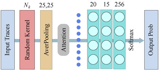
The random convolution kernel is used as the first component (i.e., as a junior encoder) to preliminarily extract features from the traces (synchronization, desynchronization, POIs/raw traces). Besides its use as an encoder, it also contributes to the dimensional reduction and denoising reduction. In order to improve the extraction efficiency and achieve a lightweight design principle, an attention mechanism is immediately appended to the junior encoder. These operations are followed by two fully-connected layers containing very few neurons, which constitutes the senior encoder of our architecture. Actually, the attention mechanism can assist the following classifier to pay more attention to the leakage features of the target intermediate operations. Finally, a classification layer (usually a softmax layer) with c classes (depending on the leakage model) and the considered cryptographic algorithm encompasses the last layers. The whole structure is shown in Figure 1.

Figure 1. The overall architecture of our SCA model.

3.2.1. Kernel

The random convolution kernel transform is a method for extracting features from time series data. It has evolved from the concept of unsupervised feature learning with random weights. With the development of convolution technology, this technique now incorporates the random initialization of various critical parameters. These parameters encompass not only the weights but also essential components such as kernel length, bias, dilation, and padding.

Number. The number of kernels is the only hyperparameter of random convolution, which is specified by the adversary and determines the output length of the junior encoder. Let $N_k$ be the number of kernels, and the output size will be $l_o=2\times N_k$ regardless of the input size of data (e.g., power traces).

Length. Commonly, the length of kernel is shorter than the time series input length. It is often sampled equiprobably from $\{7,9,11\}$. However, in practice, we found that the attack success rate for the fixed-length profiled SCA scenario is higher than for a random selection. Therefore, we choose (and fix) a length from $\{7,9,11\}$ in each complete profiling and attack phase instead of assigning different random lengths to each kernel.

Bias. The values of the biases are generated from a uniform distribution, denoted by $b_i\sim \mathcal{U}(-1,1),1\le i\le N_k$. Only biases greater than zero affect the application of kernels to time series data. As a result, similar kernels with different biases can alter the feature map by shifting values above or below zero (by a fixed amount).

Dilation. The dilation parameter acts as an input filter in the convolution operation, which can increase the receptive field. For an input X of a kernel with length $l_k$, the input with dilation d is $X_{i+j\times d}$, $0\le j\le l_k-1$. Let $l_i$ be the length of the input time series, the dilation of a kernel is sampled on an exponential scale $d=\lfloor 2^x\rfloor ,x\sim \mathcal{U}(0,A)$, where $A={log}_2{\displaystyle \frac{l_i-1}{l_k-1}}$.

Weights. This is the most important parameter. Nonetheless, the rule for generating the weights is relatively simple: all weights are generated via a normal distribution. For a single convolution kernel, each weight is set to a value $w_i$ such that $w_i\sim \mathcal{N}(0,1)$. After all the weights are set, they will be normalized as $\mathbf{W}\leftarrow \mathbf{W}-\overline{\mathbf{W}}$, where $\mathbf{W}$ denotes the weight matrix and $\overline{\mathbf{W}}={\sum }_{i=1}^{l_k}{w}_i/N_k$.

Padding. After generating each kernel, we decide whether to add a padding layer to it (chosen randomly with an equal probability) and how long this padding should be if applied. Padding means we add zeros to both at the beginning and at the end of the time series data to ensure that the middle weight of the kernel aligns with the starting point in the time series. If a kernel indeed needs padding, the padding length is calculated as follows: $\rho =\lfloor ((l_k-1)\times d)/2\rfloor$, where d denotes the dilatation and $l_k$ denotes the length of the considered kernel. Otherwise, if no padding is used, $\rho =0$. Once we determine the padding length, we can calculate the output length $l_{k_o}$ as follows: $l_{k_o}=l_i+2\rho -(l_k-1)d$, where $l_i$ is the size of the input data.

Note that all kernels have a slide window (stride) of one, and the input time series data have been normalized to have a zero mean and a standard deviation of one. For a given time series, each kernel systematically processes each data point, resulting in a feature map. A kernel K of length $l_k$ with associated weights $w_j$, $1\le j\le l_k-1$, and dilation factor d, when applied to a given time series dataset denoted as $\mathit{X}$, from position i, can be described as follows:

$${\mathit{X}}_i\ast K:=\sum _{j=0}^{l_k-1}{\mathit{X}}_{i+(j\times d)}\times w_j.$$

(8)

Finally, two features are extracted from the sequence (${\mathit{X}}_i\ast K$). Namely, the maximum value (achieved through global max pooling) denoted as $m_k$, and the proportion of positive values computed as $\left({\sum }_{{\mathit{X}}_i\ast K>0}1\right)/l_{k_o}$, denoted as $p{r}_k$. When performing these operations using a set of $N_k$ kernels, the resulting feature map for each time series has a length of $2·N_k$. We represent this output as $\mathit{H}=[m_1,p{r}_1,m_2,p{r}_2,\dots ,m_{N_k},p{r}_{N_k}]$. Since the parameters of random convolutional kernels are non-trainable, the trainable components of the entire model are reduced to only the attention mechanism and classifier. Furthermore, because the feature dimension fed into these trainable modules remains constant regardless of trace length, our approach effectively eliminates the traditional dependence between power trace length and trainable parameter quantity. This allows it to handle unprocessed raw power traces (regardless of their dimensions, POIs, or synchronization). Moreover, this method effectively mitigates the problem of rapidly increasing parameters.

3.2.2. The Attention Mechanism and Classifier

The second part of the architecture includes an attention mechanism and a classifier, which are the only components in the architecture with trainable parameters. Despite having fewer parameters compared to some current DL-based SCA models, we can still further compress it.

Before the mapped features enter the attention mechanism, we employ an average pooling layer with a kernel length and stride of 25. It is evident that, in an encrypted operation, most of the remaining power points are simply noise rather than meaningful leakage. This suggests that certain time steps contain more informative data than others. By identifying these sensitive time steps, we can simultaneously reduce the dimension and training complexity. Fortunately, the attention mechanism can play this crucial role.

Let ${\mathit{H}}^{\prime }$ be the output of the average pooling layer, then the attention mechanism works as follows:

$$\begin{array}{cc}\hfill {\mathit{s}}^{\prime }& =\mathrm{softmax}({\mathit{w}}^T·{\mathit{H}}^{\prime });\hfill \\ \hfill {\mathit{s}}^{″}& ={\mathit{H}}^{\prime }·{{\mathit{s}}^{\prime }}^T,\hfill \end{array}$$

where $\mathit{w}$ represents the trainable weight vector of a single dense layer, ${\mathit{w}}^T$ denotes the transpose, ${\mathit{s}}^{\prime }$ the attention scores, and ${\mathit{s}}^{″}$ is the output of the attention mechanism.

Lastly, we require a component to recover the intermediate encryption values and subsequently obtain the secret key. A common choice for such a classifier is a fully-connected layer (dense layer) followed by a softmax layer. The softmax function serves as an activation function, converting the output of the last layer into probability distributions ranging from 0 to 1.

The number of categories in this classification layer depends on the specific leakage model and encryption algorithm being used. For instance, if the ID model is employed, there are 256 categories, while for the HW model, there are 9 categories. In this paper, we have adopted the classification structure described in the work of Zaid et al. [21].

3.3. Training Procedure with Early Stopping

Selecting appropriate hyperparameters is a crucial and intricate aspect of deep learning model training. This includes decisions regarding the input shape, optimizer, and learning rate. In contrast to certain works (e.g., [22]) that reshape trace dimensions into 2-D structures of the form $(N,l_i,1)$ or $(N,\lfloor \sqrt{l_i}\rfloor ,l_i/\left(\lfloor \sqrt{l_i}\rfloor \right))$, we consider the trace, which represents time series data, as a 1-D shape within our architecture.

This choice of maintaining a 1-D input shape offers several advantages. First, it is better suited for the task of feature extraction using random convolutional kernels. Additionally, a 1-D input shape allows for the parallel calculation of these convolution kernels, ensuring computational speed that matches or exceeds that of commonly utilized GPU-accelerated convolution operations.

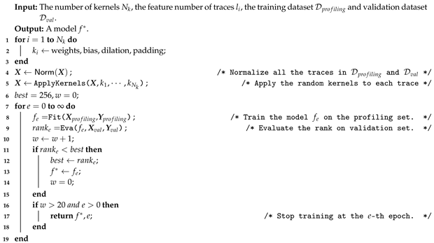
Since convolution kernels are randomly generated, the features entering the trainable part of the architecture are different every time, even for identical input traces. This variability can lead to different optimal epochs during the training process. Additionally, it is essential to ensure effective training across various datasets. One effective strategy to address these challenges is early stopping (ES). ES serves the dual purpose of preventing overfitting and preserving optimal weight parameters. Many deep learning frameworks come equipped with hardcoded early stopping mechanisms, enabling developers to either utilize them or implement custom early stopping techniques. Early stopping involves three crucial parameters: monitor, patience, and mode. The monitor parameter determines the metric to be observed during training, such as accuracy, loss, or a custom metric. Typically, these metrics are evaluated on a validation set. In the context of DL-based profiled SCA, neither loss nor accuracy serves as a suitable monitor. These metrics fail to reflect the model’s ability to successfully recover the secret key. In some cases, a model with very low accuracy (less than 0.1%) can still recover the key. Therefore, we assess the key rank and monitor it on the validation set instead of relying on loss or accuracy. The ES of the model defines the concept of improvement by observing changes in the monitor metric. Generally, the mode `max’ indicates that the DL networks are considered to improve when the metric monitor increases, while the `min’ mode is the opposite, where improvement is associated with a decrease in the metric monitor. In our architecture, we set the ES mode to `min’ because a key rank value closer to zero indicates a higher likelihood of successfully recovering the key. The patience parameter represents the number of epochs during which no improvement is tolerated before early stopping is triggered, and it is set to 20 in this method. The complete training procedure is outlined in Algorithm 1.

Algorithm 1: The overall training procedure.

3.4. Performance Analysis of Random Kernels

An interesting question is why the random convolution kernel can work well as normal convolution with trained weights. Exploring the set of optimal inputs that maximally activate the pooling unit is a good way to understand what input features are preferred by the convolutional pooling architecture.

Typically, convolutional pooling operations exhibit two characteristics: translation invariance and frequency selectivity. Therefore, to prove that a random convolutional kernel has the same efficiency as a regular convolutional pooling layer, it is only necessary to prove that random convolutional kernels also possess these two features.

By using pooling operations, this architecture naturally shows translation invariance, and itself should be a family of optimal inputs. Then, the question is whether the random convolution kernel with the two pooling operations also has the frequency selectivity. Through frequency domain analysis, the work of Andrew et al. [23] provided an idea to answer it. In their theory, a 2D “circular” (kernels sliding on every position in the rolled data) convolutional square pooling architecture has the optimal input as

$$x^{opt}[m,s]={\displaystyle \frac{\sqrt{2}}{n}}cos\left({\displaystyle \frac{2\pi mv}{n}}+{\displaystyle \frac{2\pi sh}{n}}+\varphi \right),$$

(9)

where n represents input dimension, v vertical frequencies, and h horizontal frequencies, $\varphi$ an unspecified phase. In particular, let the filter f be formed by zero-padding f to size $n\times n$. Then $(v,h)$ is the frequency pair with amplitude equal to the maximum amplitude of any frequency in f. Moreover, for a 2D “valid” convolution (kernels sliding on the positions within unrolled data), there exists a sinusoidal input $x^{sin}$ that is near optimal for the activation of pooling units such that

$$x^{sin}[m,s]={\displaystyle \frac{\sqrt{2}}{n}}cos\left({\displaystyle \frac{2\pi mv}{n}}+{\displaystyle \frac{2\pi sh}{n}}+\varphi \right).$$

(10)

Then for all $x(\parallel x\parallel =1)$, the following inequality holds.

$$p_v\left(x^{sin}\right)\ge p_v\left(x\right)-K{n}^{-1},$$

where $K=4k^3{\parallel f\parallel }^2$ does not depend on n. The two equations (9) and (10) are sufficient to illustrate that the frequency of the optimal input is the frequency of maximum magnitude in the filter f. Namely, the architecture is frequency selective and translation invariant.

The same characteristics also exist in random convolutional kernels. Considering an 1D convolutional kernel (or filter) $f\in {\mathbb{R}}^k,k<n$, the activation of the pooling unit is determined by the kernel f and input x, then computing the average of the sum of the output of the convolution layer. Since convolution operation is linear, the problem about optimal input features can be seen as a matrix norm problem, i.e., to obtain the solution of x which makes ${\parallel C\parallel }_1$ maximum. The matrix C is flattened by the convolutional kernel and it is a Toeplitz matrix. According to the norm inequality, we have ${\parallel Cx\parallel }_1\le \sqrt{n}{\parallel Cx\parallel }_2$. Then the problem can further transform to solve the optimization problem of ${max}_{x\in {\mathbb{R}}^n,x\ne 0}{\displaystyle \frac{x^{*}{C}^{*}Cx}{x^{*}x}}$, where “$x^{*}$” means the transpose operation. Obviously, this is a semi-positive definite quadratic form, and its solution is the eigenvector related to the maximum eigenvalue of C. We reparameterize the optimization problem into a solution matrix $C^{*}C$, where the eigenvalues and eigenvectors can be directly read from the diagonalization matrix to obtain an analyzable solution. Introduce a 2D discrete Fourier transform matrix F, such that $z=Fx$:

$$\begin{array}{cc}\hfill {\displaystyle \frac{x^{*}{C}^{*}Cx}{x^{*}x}}& ={\displaystyle \frac{z^{*}F{C}^{*}C{F}^{*}z}{z^{*}F{F}^{*}z}}\hfill \\ \hfill & ={\displaystyle \frac{z^{*}F{C}^{*}{F}^{*}FC{F}^{*}z}{z^{*}z}}={\displaystyle \frac{z^{*}{\Lambda }^{*}\Lambda z}{z^{*}z}}.\hfill \end{array}$$

Then there is a modified optimization problem ${max}_{z\in {\mathcal{R}}^{n^2},z\ne 0}$ ${\displaystyle \frac{z^{*}{|\Lambda |}^{2}z}{z^{*}z}},\mathit{\text{s.t.}}{F}^{*}z\in \mathcal{R}$. Consequentially, the solution $z_j$ is given by

$$z_j=\left\{\begin{array}{cc}{\displaystyle \frac{a_{\left|j\right|}}{\sqrt{2}}}{e}^{i\mathrm{sgn}\left(j\right){\varphi }_{\left|j\right|}}\hfill & {\lambda }_j\in max\lambda ,\hfill \\ 0\hfill & \mathrm{otherwise}.\hfill \end{array}\right.$$

Converting z to the spatial domain can obtain Equations (9) and (10). Therefore, one-dimensional convolutional pooling architecture also maintains the frequency as selective and translation as invariant. In addition, the use of max pooling units is to better handle noise in power consumption.

3.5. Complexity Analysis

The computational complexity of the architecture can be estimated from two parts: the complexity of the non-trainable random kernels and the complexity of the trainable classifier. The random kernel transform only relies on the number of kernels $N_k$ and the length of traces in the dataset. Formally, its complexity is $O(N_k·(N_p+N_a)·l_i)$. The symbol $N_k$ denotes the number of generated convolutional kernels, where each kernel extracts two power consumption feature values from each trace. $N_p$ represents the profiling set size, i.e., the number of power traces used during the training phase. Similarly, $N_a$ indicates the attack set size, specifying the number of traces available to the adversary for key recovery during the attack phase. Finally, $l_i$ corresponds to the number of power samples in each individual power trace, which may either be preprocessed (through POIs, denoising, etc.) or remain raw traces. This process only involves repeated multiplications and additions, so its complexity is determined by the input length and the convolution length, with a maximum convolution length of 11, which can be regarded as a constant without impacting on the overall complexity.

The classifier, as explained above, is the trainable component of the model, and it follows a lightweight principle. The complexity of this process is mainly dictated by the sum of trainable parameters of each layer. As shown in Table 1, the trainable components have two softmax layers, four dense layers, an average-pooling layer, and a multiply layer. The only trainable parameters are thus the ones for the dense layers. Similarly, the number of trainable parameters only relies on the number of kernels and the number of categories (determined by the leakage model). The average-pooling reduces the length of extracted features from the random kernel layers by 25 times, i.e., features with length $2N_k$ are turned into features of length $\lfloor 2N_k/25\rfloor$.

Table 1. The parameters of our architecture.

Hyperparameter Type	Hyperparameter Shape	Complexity *
Random kernel	time series length ($l_i$)	$N_k·l_i+3N_k$
	number of kernels ($N_k$)
Attention	averagePooling1D ($\lfloor 2N_k/25\rfloor$)	0
	dense (1)	21
	softmax (1)	0
	multiply (20)	0
Classifier	dense (20)	420
	dense (15)	315
	dense (c)	$15c+c$
	softmax (c)	0

* The total spatial complexity is $N_k·(N_p+N_a)·l_i+\left(\lfloor 2N_k/25\rfloor \right)·(21+420+315+15c+c)$, where $N_p$ is the size of the profiling set, $N_a$ is the size of the attack set and c is the number of classes.

For example, if the number of kernels is 260, the length of features after random kernel layers is 20. Then, the dense layer processes $1\times 20+1$ weights. In the classifier, there are 3 dense layers with parameters $\{20,15,c\}$, which induce the number of weights: $(20\times 20+20)+(20\times 15+15)+(15c+c)=420+315+15c+c$. For the AES algorithm, if the leakage model is ID, there are 4831 weights; otherwise, if the leakage model is HW, the number of weights is 879. Finally, the complexity of the trainable part is given by $O(N_p·N_k^2·c)$.

Moreover, the time complexity of the whole architecture is also analyzed as follows. Firstly, the time consumption of the non-trainable part could be ignored because the random kernel part is used as a transformer on traces. This means that the transformer only needs to be applied once, and the transformed power traces can be stored. Secondly, for the trainable part, due to the constant input length, the time consumption of this part only relies on the number of training traces, rather than being determined by both the number of training traces and the number of power points per trace. Therefore, the architecture eliminates the dependency between the number of power points (trace length) and the number of trainable parameters, and this is the reason why it can directly deal with million-dimensional raw power traces.

4. Experiments and Analysis

In this section, we evaluate our architecture by conducting the profiling and attack phases on various datasets, including ASCADv1, AES_HD, AES_RD, and CHES CTF. Our results showcase its competitiveness in metrics such as profiling cost, $T_{GE0}$, and adaptability of raw traces. We offer an overview of the datasets, including power file organization, metadata (plaintext, ciphertext, key, etc.), and their variations. Then, we outline our experimental setups and present the results obtained from different datasets.

4.1. Datasets

ASCAD. The ASCAD dataset is a benchmark for DL-based SCA research. It is sampled from the ATMega8515-board, which implements a masked AES-128 [6].

ASCAD_fixed_key (ASCAD_f). This subset includes 50,000 profiling traces and 10,000 attack traces. Each trace contains 700 pre-selected features using a signal-to-noise ratio from the original 100,000-dimensional trace. The labels for these trace intervals are determined by the third S-box of the first round of AES, and the key remains fixed.

ASCAD_variable_key (ASCAD_r). This subset comprises 200,000 profiling traces with variable keys and plaintexts. Additionally, it contains 100,000 traces for the attack phase with fixed keys and random plaintexts, each trace including 1400 points of interest.

ASCAD_raw_traces. This dataset serves as the foundational source for both ASCAD_f and ASCAD_r. It contains all the raw traces, including 100,000 time points and associated metadata for each trace.

AES_HD. The traces in the AES_HD dataset are sampled from Xilinx Virtex-5 FPGA, which carries out an unprotected AES-128 implementation [24]. Unlike the other datasets, its traces record the AES decryption procedure instead of the encryption process. The labels are then calculated by the 12-th byte and 8-th byte of ciphertexts $c_i^j$, i.e., $\varphi (c_i,k_i)={sbox}^{-1}(c_i^{11}\oplus k_i)\oplus c_i^7$. We used and analyzed the compressed AES_HD dataset.

AES_RD. AES_RD was used to study random delay countermeasures, in which the traces are collected from an 8-bit ATMEL AVR platform executing an AES-128 encryption, and we used the pre-processed dataset as analyzed in [21].

CHES CTF. The CHES CTF is the dataset containing traces generated for the CHES 2018 AES-128 CTF challenge. It provides six different subsets (42,000 traces), where a single reduced version (45,000 traces) is used in the experiments. The reduced version is used in the AISY framework and has already been pre-processed [25].

4.2. Setups and Environments

First, we need to determine the hyperparameters for our architecture. Luckily, we only have three hyperparameters to worry about because of our design, which employs a non-training structure and a lightweight classifier. These hyperparameters are the number of kernels (denoted as $N_k$), the learning rate of the classifier ($l_r$), and the batch size. To optimize the learning rate, we can use cyclical learning rate (CLR) technology [26,27]. We set the batch size to 50, following best practices from deep learning-based SCA model training methods [16,20].

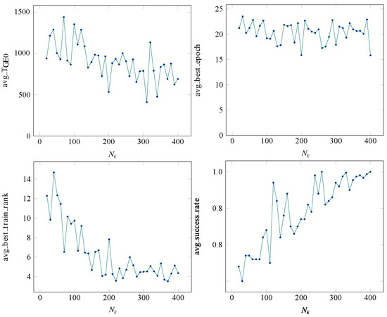
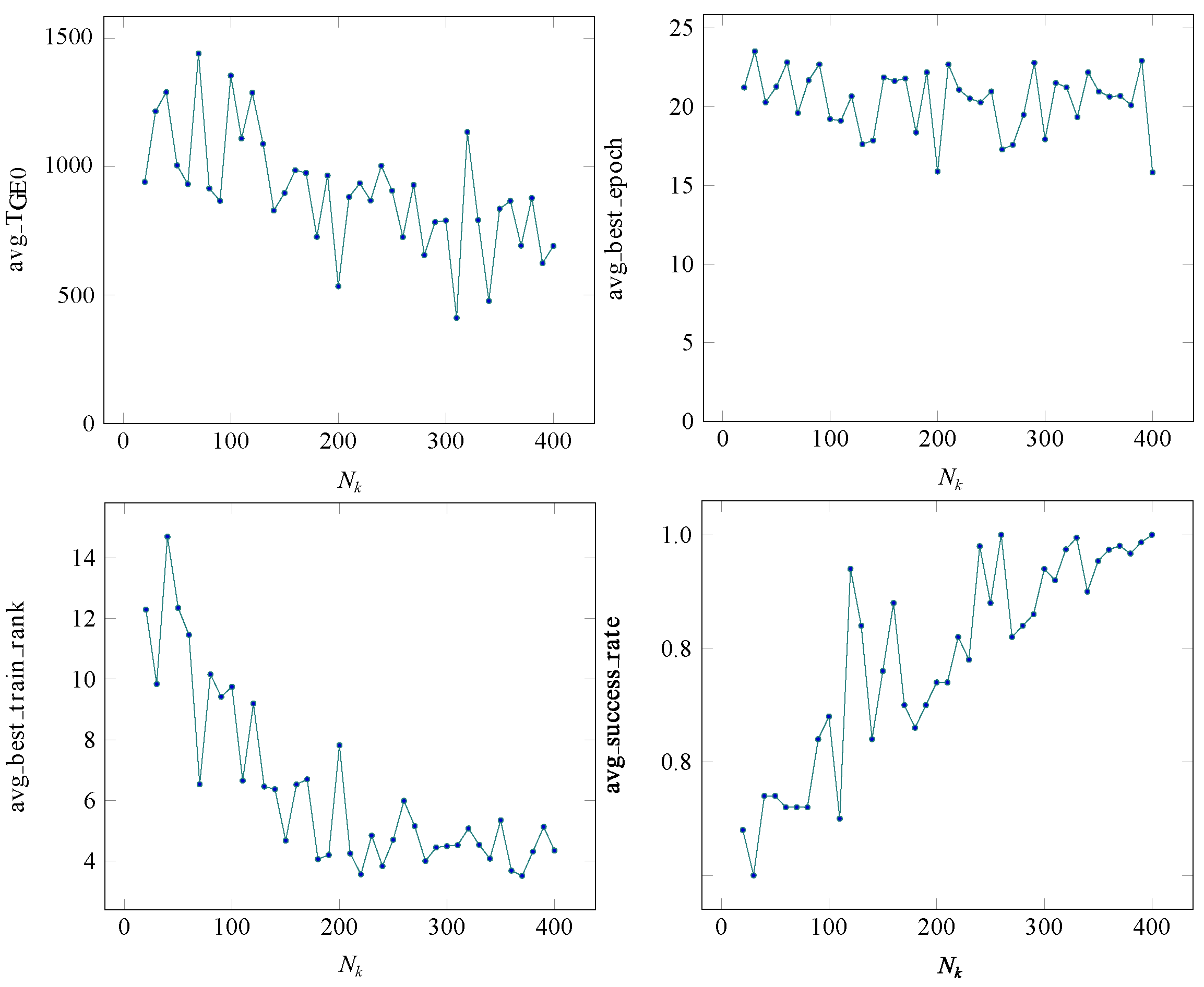
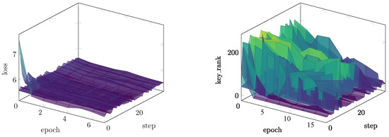
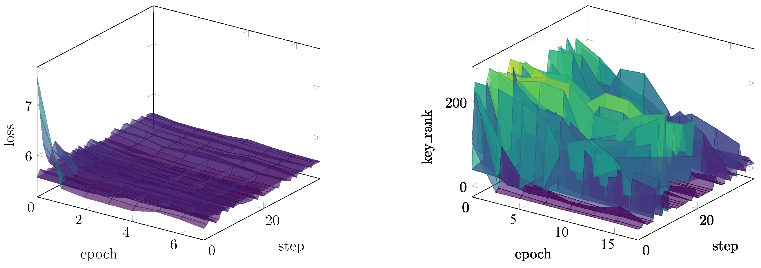
Now, let us focus on the number of kernels $N_k$. We conduct an experiment where we increase the number of kernels in increments of 10, ranging from 20 to 400. This approach adheres to the principle of minimizing the number of features in the input classifier. We repeat this experiment 100 times for each kernel. For this experiment, we use traces from the ASCAD dataset, where we select 1500 points of interest from the raw power trace file “ATMega8515_raw_traces.h5”. The selection was based on the signal-noise-ratio (SNR) (the SNR is sometimes referred as the F-Test) [28]. For a noisy observation $X_t$ at time sample t of an event Y, it is defined as $Var\left[E\left[X_t\right|Y]\right]/E\left[Var\left[X_t\right|Y]\right]$. The training dataset, denoted as ${\mathcal{D}}_{train}$, consists of 15,000 traces, and the attack dataset, denoted as ${\mathcal{D}}_{attack}$, contains 5000 traces. Notably, there is no separate testing dataset in this experiment because it is not required to select an optimal model from the test dataset. In this experiment, we evaluate four metrics: the average value of $T_{GE0}$, the average best epoch, the average best training key rank, and the average attack success rate. Finally, $T_{GE0}$ stabilizes around 500 after $N_k$ reaches 200, and the average best training epoch is essentially 20 regardless of the value of $N_k$. The average best training rank and the average attack success rate are more closely related to $N_k$. From the results in Figure 2, we observe that the best $N_k$ is about 260, which induces a good trade-off for the number of trainable parameters and the attack efficiency. In addition, we also record the loss and rank changes for each epoch and batch in a single training phase, which is shown in Figure 3.

Figure 2. The average $T_{GE0}$, best epoch, best training key rank, and attack success rate.

Figure 3. The loss and rank changes with epochs and batches (Viridis colormap is used to represent changes in numerical values from large to small).

Upon determining the hyperparameter $N_k$, we provide the detailed setups for datasets in Table 2. In this description, we include the attack byte (indices of bytes where the correct key is at) and the decimal values of correct keys. We conducted experiments on the ASCAD, AES_HD, AES_RD and CHES CTF datasets. As pointed out above, there are several variants in the ASCAD dataset. We used the previously described subsets ASCAD_f, ASCAD_r, where we also considered their desynchronization level. Notice also that the traces in ASCAD_f_raw are full power time points (100,000 points) without any SNR selection. To control the operation time of the random convolution kernels, the profiling traces are reduced to 4500 compared with other ASCAD variants. Similarly to ASCAD datasets, we analyzed the AES_HD dataset, where we manually added random desynchronization with a level of 50 and 100. Note that the desynchronization level is indicated by appending “_desyncX” for $X\in \{50,100\}$ to the corresponding dataset.

Table 2. Details of the datasets.

Dataset	Trace Length	Profiling Traces	Attack Traces	Attack Byte
ASCAD_f	700	15,000	5000	2 (224)
ASCAD_f_desync50	700	15,000	5000	2 (224)
ASCAD_f_desync100	700	15,000	5000	2 (224)
ASCAD_f_raw	100,000	4500	5000	2 (224)
ASCAD_r	1400	15,000	5000	2 (34)
AES_HD	1250	15,000	5000	0 (0)
AES_HD_desync50	1250	15,000	5000	0 (0)
AES_HD_desync100	150	15,000	5000	0 (0)
AES_RD	3500	15,000	5000	0 (43)
CHES CTF	2200	15,000	5000	2 (94)

Experimental platform. Our architecture requires the training of a minimal number of hyperparameters, rendering GPU acceleration measures unnecessary. Instead, we rely solely on the computational capacity of the CPU. All experiments were carried out on a PC with a 12th Gen Intel ^® Core^TM i5-12500H × 16 CPU, equipped with a 16.0 GB RAM, and running 64-bit Ubuntu 22.04.1 LTS. Remarkably, each experiment on a dataset variant takes only about 20–30 s to finish.

4.3. Experimental Results

For each dataset, we present the experimental results, which include training loss, validation loss, and validation key rank. In order to improve training efficiency, we used the Early Stopping (ES) strategy. In experimental figures, we will indicate the epochs using dotted lines. At the same time, the values of $T_{GE0}$ are compared on each dataset. Finally, we compare these two metrics and trainable parameters with some state-of-the art architectures.

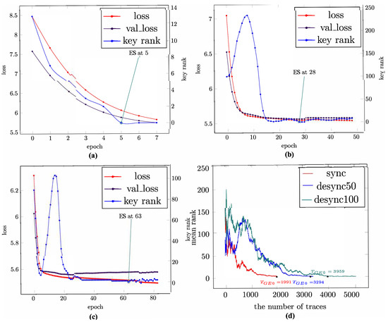
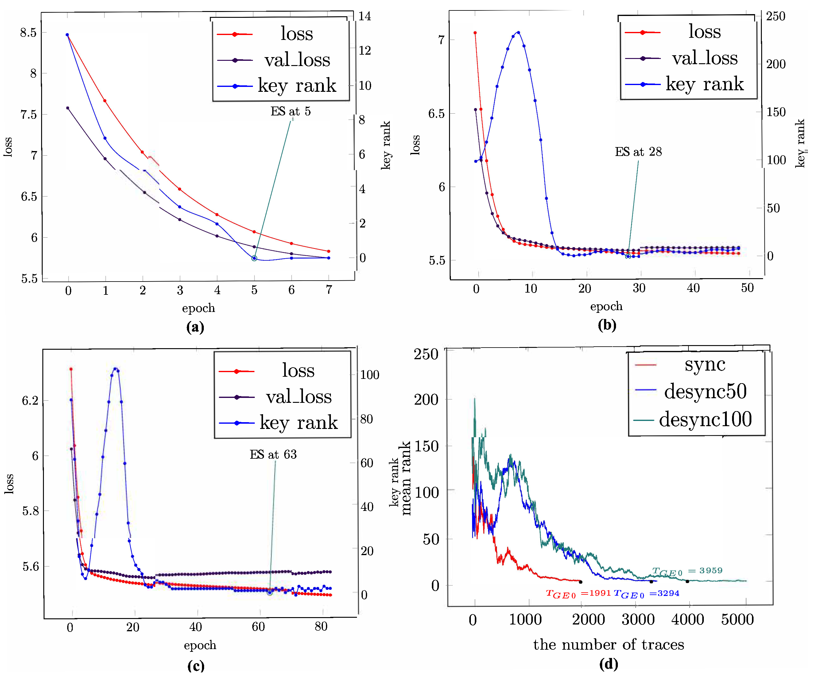
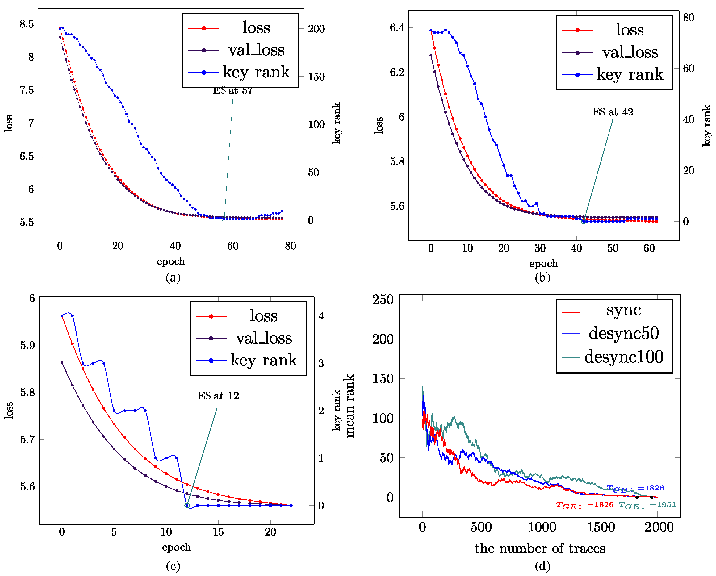
For the AES_HD dataset, we conduct an experiment on the synchronization traces set, then manually add desynchronizing noise with two levels of 50 and 100.Then, we record the training loss, validation loss and the metrics $T_{GE0}$ of these experiments. In Figure 4, we depict the changes in loss (red) and validation loss (gray) using the left y-axis as a reference, and plot the key rank changes (blue) using the right y-axis. Moreover, to verify $T_{GE0}$, all the GEs and the number of traces for the key are recorded. From these result, we can see that the learning curve is very smooth and only a few epochs are needed to learn about the power leakage. In addition, its attack efficiency is also good, yielding $T_{GE0}=1991$.

Figure 4. The experimental result on AES_HD dataset: (a) synchronization, (b) desync50, (c) desync100, (d) $T_{GE0}$.

Then, we added two different levels of desynchronization noise to the traces of the AES_HD dataset. We observe that the key ranks have an obvious fluctuation, so it takes more epochs to train (Figure 4b and Figure 4c with an ES of 28 and 63, respectively), as adding desynchronization noise. In addition, the required number of traces for a successful attack (Figure 4d) is slightly greater than in the synchronization scenario.

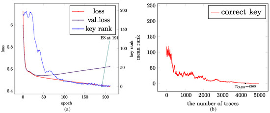
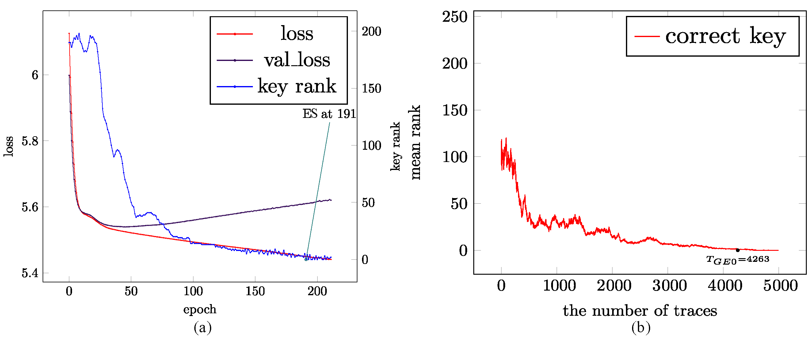
In the AES_RD dataset, the power traces come with an inherent desynchronization noise. Therefore, it is sufficient to conduct only one experiment. The experimental results are shown in Figure 5. Compared with the AES_HD dataset, the model needs more epochs (ES at 191) for AES_RD. In total, it takes about 37 s and 190 ms per epoch. Note also that the loss and key rank reduction on AES_RD is similar to the ones on the AES_HD dataset with 100-level desynchronization.

Figure 5. The experimental result for the AES_RD dataset, where (a,b) show the learning state and the evaluation of the attack.

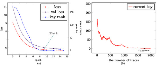
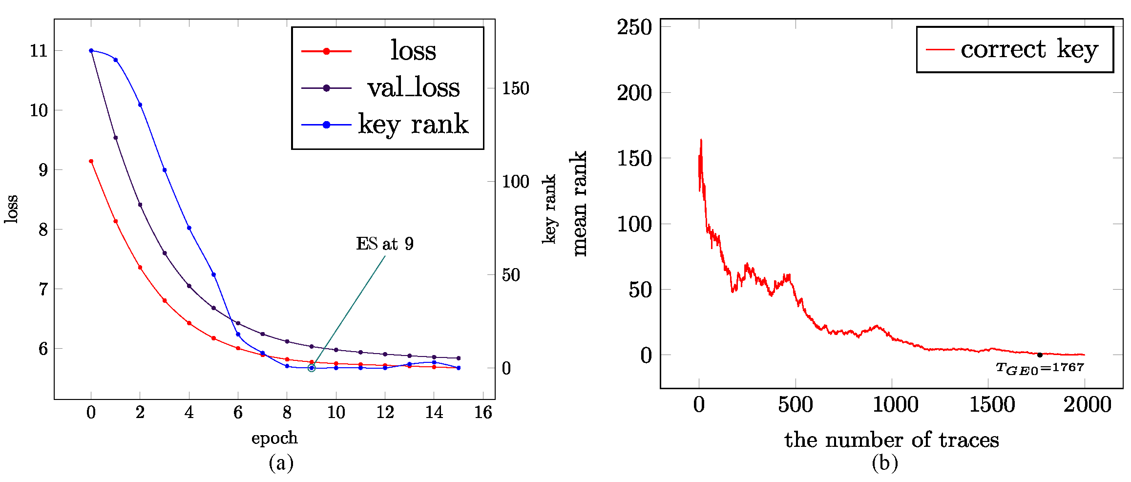
We performed an experiment on CHES CTF dataset. The result shows that the model was trained on the 9th epoch with an average time of 350 ms per epoch. Figure 6 depicts the details of the experiment.

Figure 6. The experiment on the CHES CTF dataset; (a,b) show the training situations and the evaluation result.

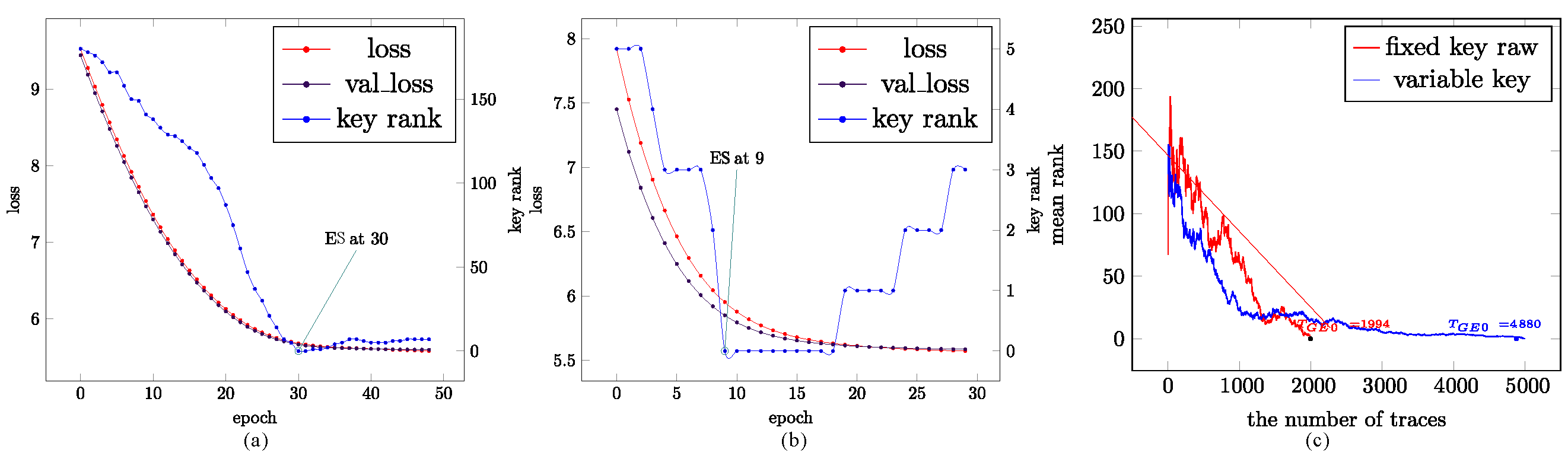
ASCAD is the largest dataset used in this paper. We will focus on the fixed key version (ASCAD_f) and on the variable key version (ASCAD_r). Therefore, the experimental results are organized into two parts, based on whether the training key is fixed or not. First, we show the results for a fixed key with synchronization in Figure 7a. The experimental results of the fixed key and desynchronization version are shown in the Figure 7b,c.

Figure 7. The experiment on the ASCAD_f dataset: (a) synchronization, (b) desync50, (c) desync100, (d) $T_{GE0}$.

In addition to the above versions, we also conducted experiments on the ASCAD_raw dataset for the synchronization version, without any preprocessing. This is referred as the fixed key and raw version. The result is shown in Figure 8a. It is worth noting that although there are no POIs, the model can still properly learn leaked knowledge in a very short time. The result of the variable key version of ASCAD is shown in Figure 8b.

Figure 8. The experimental result of (a) the fixed-key raw version the ASCAD dataset, (b) the variable key version of the ASCAD_r dataset, (c) $T_{GE0}$.

4.4. Comparison and Analysis

To some extent, the operation of random convolution kernels may appear somewhat similar to power consumption preprocessing based on wavelet transform. However, in practice, we cannot simply regard the role of random convolution kernels as merely a preprocessing technique. To elaborate on this perspective, we first summarize several wavelet transform-based side-channel analysis methods, such as those in [29,30,31] In the work of [29], wavelet transform and principal component analysis (PCA) were jointly employed for power trace preprocessing. By utilizing neural networks trained on the processed power traces, they achieved approximately 20% improvement in success rate. Similarly, the study in [30] leveraged both wavelet transform and inverse wavelet transform to obtain denoised traces, upon which CPA was performed to recover the secret key. The literature [31] integrates wavelet transform with convolutional networks to propose a novel dedicated feature extraction layer. By designing trainable parameters to optimize wavelet scales, this method achieves competitive performance on the ASCAD dataset. The commonality among these approaches lies in their application of wavelet transform for preprocessing power traces during attacks, primarily aimed at denoising (i.e., enhancing the Signal-to-Noise Ratio, SNR). In contrast, another strategy involves transforming 1D power traces into two-dimensional image representations using wavelet transform (or Short-Time Fourier Transform, STFT), followed by leveraging mature deep learning architectures from the image processing domain to learn leakage features, as demonstrated in [32,33].

Due to fundamental differences in evaluation metrics and methodologies, a direct comparison between these approaches [29,30,31,32,33] and our proposed method cannot be fully established. Additionally, the functionality of random convolutional kernels inherently differs from wavelet transform—they serve dual functions of feature extraction and noise reduction through an irreversible process (enabled by convolution-pooling operations). Therefore, we restrict our evaluation to their common operational dimension, specifically the efficiency in power trace processing, while deliberately excluding their differential impacts on attack effectiveness. The results are provided in Table 3.

Table 3. The processing efficiency of several wavelet transforms (fast Fourier transform) and random convolution kernels.

Pre-Processing Technique	Input (Trace) Length	Output (Feature) Length	Time Cost/s (1000 Traces)
Wavelet+PCA [29,30]	700	520	6.84963298
	1250		8.00765491
	1400		8.87215233
	2200		8.32040954
	3500		9.62530255
	100,000		41.92533708
Time-Frequency image [32,33] *	700	$224\times 224$/$51\times 46$	0.06076002/0.06228614
	1250		0.24854016/0.30057955
	1400		0.35778213/0.38010383
	2200		1.24332047/1.30320311
	3500		6.13667226/7.13198972
	100,000		-/-
Random Convolution Kernels	700	520	0.41842961
	1250		0.72135997
	1400		0.77635646
	2200		1.18555427
	3500		1.77288055
	100,000		46.68730211

* Ref. [32] uses STFT transform whereas [33] utilizes wavelet transform, resulting in two distinct numerical metrics within the evaluation outcomes.

Finally, we compared our architecture with the State-of-the-Art (SoA) methods in terms of performance of trainable parameters, training duration, and the minimum number of samples required to recover the real key (Table 4). The number of profiling traces and number of parameters are two important factors that affect the time cost of the profiling phase.

Table 4. Comparison of our architecture with the SoAs.

Model	Dataset Name	Num. Pro. Traces	Num. Param.	Time/(100 Batches)	${\mathit{T}}_{\mathit{GE}0}$
[6]	ASCAD_f	50,000	66,652,544	244.6 s	782
	ASCAD_f_desync100				8033
[15]	ASCAD_f	10,000	47,778,176	167.7 s	3860
[16]	ASCAD_f	50,000	79,695	2.10 s	4050
	ASCAD_r		151,375	3.92 s	3684
	CHES CTF		233,295	6.31 s	1458
[31]	ASCAD_f	50,000	66,646,208	230.5 s	133
	ASCAD_f_desync100		66,646,208		5512
Ours	ASCAD_f	15,000	4852	0.1173323 s	1826
	ASCAD_f_raw			0.0635662 s	1948
	ASCAD_r			0.3135437 s	4880
	CHES CTF			0.1166667 s	1767
	AES_HD			0.0676667 s	1974
	AES_RD			0.0681399 s	1953

In these methods, the work [6] made significant contributions by providing the ASCAD dataset and also examining the application of MLP, CNN, and other classical models in side-channel attacks. The study [15] introduced adversarial learning techniques and randomized data augmentation methods, with the goal of learning leakage characteristics using fewer profiling traces. This approach can be conceptually viewed as improving feature extraction efficiency and reducing training overhead by decreasing the required training set size. The literature [16] proposed transforming the classification model in DL-SCA into a regression model through a specially designed label-distribution-based loss function, which simultaneously reduced both the necessary training epochs and the number of trainable parameters compared to conventional approaches. The literature [31] integrates wavelet transform with convolutional networks to propose a novel dedicated feature extraction layer. By designing trainable parameters to optimize wavelet scales, this method achieves competitive performance. The results show that our architecture exhibits significant advantages in both the above factors so that the time cost in the profiling phase is reduced by hundreds of times compared to other approaches.

Moreover, the trainable parameters of our model are constant for traces of different datasets and feature points, which is also the reason why the training speed of the model is much faster than that of conventional SoA DL-based SCA models.

5. Conclusions

In this paper, we address the problem of exponentially increased training time costs as more features are selected from raw power traces. By employing random kernel convolution, a lightweight architecture that integrates attention mechanisms is proposed for DL-based profiled SCA. Compared with previous methods, our architecture achieves the constantization of trainable parameters when the number of profiling traces is fixed. Furthermore, the performance and complexity of the random convolution kernels are analyzed. Finally, our findings on multiple datasets demonstrate that this model effectively reduces the number of trainable parameters and enhances the learning phase across various scenarios. In future work, we aim to extend this model to handle more complex masking implementations, such as inner masking and affine masking.

References

- Kocher, P.C. Timing Attacks on Implementations of Diffie-Hellman, RSA, DSS, and Other Systems. In Proceedings of the Advances in Cryptology—CRYPTO’96, 16th Annual International Cryptology Conference, Santa Barbara, CA, USA, 18–22 August 1996; Springer: Berlin/Heidelberg, Germany, 1996; pp. 104–113. [Google Scholar]
- Kocher, P.C.; Jaffe, J.; Jun, B. Differential power analysis. In Proceedings of the Advances in Cryptology—CRYPTO’99: 19th Annual International Cryptology Conference, Santa Barbara, CA, USA, 15–19 August 1996; Springer: Berlin/Heidelberg, Germany, 1999; pp. 388–397. [Google Scholar]
- de la Fe, S.; Park, H.B.; Sim, B.Y.; Han, D.G.; Ferrer, C. Profiling Attack against RSA Key Generation Based on a Euclidean algorithm. Information 2021, 12, 462. [Google Scholar] [CrossRef] [Scilit]
- Maghrebi, H.; Portigliatti, T.; Prouff, E. Breaking Cryptographic Implementations Using Deep Learning Techniques. In Proceedings of the Security, Privacy, and Applied Cryptography Engineering: 6th International Conference, Hyderabad, India, 14–18 December 2016; Springer: Berlin/Heidelberg, Germany, 2016; pp. 3–26. [Google Scholar]
- Kim, J.; Picek, S.; Heuser, A.; Bhasin, S.; Hanjalic, A. Make Some Noise. Unleashing the Power of Convolutional Neural Networks for Profiled Side-channel Analysis. IACR Trans. Cryptogr. Hardw. Embed. Syst. 2019, 2019, 148–179. [Google Scholar] [CrossRef] [Scilit]
- Benadjila, R.; Prouff, E.; Strullu, R.; Cagli, E.; Dumas, C. Deep learning for side-channel analysis and introduction to ASCAD database. J. Cryptogr. Eng. 2020, 10, 163–188. [Google Scholar] [CrossRef] [Scilit]
- Picek, S.; Samiotis, I.P.; Kim, J.; Heuser, A.; Bhasin, S.; Legay, A. On the Performance of Convolutional Neural Networks for Side-Channel Analysis. In Proceedings of the Security, Privacy, and Applied Cryptography Engineering: 8th International Conference, Kanpur, India, 15–19 December 2018; Springer: Berlin/Heidelberg, Germany, 2018; pp. 157–176. [Google Scholar]
- Li, L.; Ou, Y. A deep learning-based side channel attack model for different block ciphers. J. Comput. Sci. 2023, 72, 102078. [Google Scholar] [CrossRef] [Scilit]
- Wu, L.; Perin, G.; Picek, S. The Best of Two Worlds: Deep Learning-assisted Template Attack. IACR Trans. Cryptogr. Hardw. Embed. Syst. 2021, 2022, 413–437. [Google Scholar] [CrossRef] [Scilit]
- Perin, G.; Wu, L.; Picek, S. Exploring Feature Selection Scenarios for Deep Learning-based Side-Channel Analysis. IACR Trans. Cryptogr. Hardw. Embed. Syst. 2022, 2022, 828–861. [Google Scholar] [CrossRef] [Scilit]
- Acharya, R.Y.; Ganji, F.; Forte, D. Information Theory-based Evolution of Neural Networks for Side-channel Analysis. IACR Trans. Cryptogr. Hardw. Embed. Syst. 2023, 2023, 401–437. [Google Scholar] [CrossRef] [Scilit]
- Hajra, S.; Chowdhury, S.; Mukhopadhyay, D. EstraNet: An Efficient Shift-Invariant Transformer Network for Side-Channel Analysis. Cryptology ePrint Archive, Paper 2023/1860. 2023. Available online: https://eprint.iacr.org/2023/1860 (accessed on 6 December 2023).
- Ahmed, A.A.; Salim, R.A.; Hasan, M.K. Deep Learning Method for Power Side-Channel Analysis on Chip Leakages. Elektron. Elektrotechnika 2023, 29, 50–57. [Google Scholar] [CrossRef] [Scilit]
- Zhang, Z.; Ding, A.A.; Fei, Y. A Guessing Entropy-Based Framework for Deep Learning-Assisted Side-Channel Analysis. IEEE Trans. Inf. Forensics Secur. 2023, 18, 3018–3030. [Google Scholar] [CrossRef] [Scilit]
- Liu, A.; Wang, A.; Sun, S.; Wei, C.; Ding, Y.; Wang, Y.; Zhu, L. CL-SCA: Leveraging Contrastive Learning for Profiled Side-Channel Analysis. Cryptology ePrint Archive, Paper 2024/049. 2024. Available online: https://eprint.iacr.org/2024/049 (accessed on 15 January 2024).
- Wu, L.; Weissbart, L.; Krček, M.; Li, H.; Perin, G.; Batina, L.; Picek, S. Label Correlation in Deep Learning-Based Side-Channel Analysis. IEEE Trans. Inf. Forensics Secur. 2023, 18, 3849–3861. [Google Scholar] [CrossRef] [Scilit]
- Ou, Y.; Li, L. Research on a high-order AES mask anti-power attack. IET Inf. Secur. 2020, 14, 580–586. [Google Scholar] [CrossRef] [Scilit]
- Dempster, A.; Petitjean, F.; Webb, G. ROCKET: Exceptionally fast and accurate time series classification using random convolutional kernels. Data Min. Knowl. Discov. 2020, 34, 1454–1495. [Google Scholar] [CrossRef] [Scilit]
- Salehinejad, H.; Wang, Y.; Yu, Y.; Jin, T.; Valaee, S. S-Rocket: Selective Random Convolution Kernels for Time Series Classification. arXiv 2022, arXiv:cs.LG/2203.03445. [Google Scholar]
- Rijsdijk, J.; Wu, L.; Perin, G.; Picek, S. Reinforcement learning for hyperparameter tuning in deep learning-based side-channel analysis. IACR Trans. Cryptogr. Hardw. Embed. Syst. 2021, 2021, 677–707. [Google Scholar] [CrossRef] [Scilit]
- Zaid, G.; Bossuet, L.; Habrard, A.; Venelli, A. Methodology for efficient CNN architectures in profiling attacks. IACR Trans. Cryptogr. Hardw. Embed. Syst. 2020, 2020, 1–36. [Google Scholar] [CrossRef] [Scilit]
- Gupta, P.; Drees, J.P.; Hüllermeier, E. Automated Side-Channel Attacks using Black-Box Neural Architecture Search. Cryptology ePrint Archive, Paper 2023/093. 2023. Available online: https://eprint.iacr.org/2023/093 (accessed on 14 January 2024).
- Saxe, A.M.; Koh, P.W.; Chen, Z.; Bhand, M.; Suresh, B.; Ng, A.Y. On random weights and unsupervised feature learning. ICML 2011, 2, 6. [Google Scholar]
- Picek, S.; Heuser, A.; Jovic, A.; Bhasin, S.; Regazzoni, F. The Curse of Class Imbalance and Conflicting Metrics with Machine Learning for Side-channel Evaluations. IACR Trans. Cryptogr. Hardw. Embed. Syst. 2019, 2019, 209–237. [Google Scholar] [CrossRef] [Scilit]
- Perin, G.; Wu, L.; Picek, S. AISY—Deep Learning-based Framework for Side-channel Analysis. Cryptology ePrint Archive, Paper 2021/357. 2021. Available online: https://eprint.iacr.org/2021/357 (accessed on 18 March 2021).
- Smith, L. A disciplined approach to neural network hyper-parameters: Part 1 – learning rate, batch size, momentum, and weight decay. arXiv 2018, arXiv:cs.LG/1803.09820. [Google Scholar]
- Smith, L.; Topin, N. Super-Convergence: Very Fast Training of Neural Networks Using Large Learning Rates. arXiv 2018, arXiv:cs.LG/1708.07120. [Google Scholar]
- Fisher, R.A. On the Mathematical Foundations of Theoretical Statistics. Philos. Trans. R. Soc. 1922, 222, 309–368. [Google Scholar]
- Saravanan, P.; Kalpana, P.; Preethisri, V.; Sneha, V. Power analysis attack using neural networks with wavelet transform as pre-processor. In Proceedings of the 18th International Symposium on VLSI Design and Test, Coimbatore, India, 16–18 July 2014; pp. 1–6. [Google Scholar] [CrossRef] [Scilit]
- Ai, J.; Wang, Z.; Zhou, X.; Ou, C. Improved wavelet transform for noise reduction in power analysis attacks. In Proceedings of the 2016 IEEE International Conference on Signal and Image Processing (ICSIP), Beijing, China, 13–15 August 2016; pp. 602–606. [Google Scholar] [CrossRef] [Scilit]
- Bae, D.; Park, D.; Kim, G.; Choi, M.; Lee, N.; Kim, H.; Hong, S. Autoscaled-Wavelet Convolutional Layer for Deep Learning-Based Side-Channel Analysis. IEEE Access 2023, 11, 95381–95395. [Google Scholar] [CrossRef] [Scilit]
- Yang, G.; Li, H.; Ming, J.; Zhou, Y. Convolutional Neural Network Based Side-Channel Attacks in Time-Frequency Representations. In Smart Card Research and Advanced Applications; Bilgin, B., Fischer, J.B., Eds.; Springer: Cham, Switzerland, 2019; pp. 1–17. [Google Scholar]
- Garg, A.; Karimian, N. Leveraging Deep CNN and Transfer Learning for Side-Channel Attack. In Proceedings of the 2021 22nd International Symposium on Quality Electronic Design (ISQED), Santa Clara, CA, USA, 7–8 April 2021; pp. 91–96. [Google Scholar] [CrossRef] [Scilit]
Disclaimer/Publisher’s Note: The statements, opinions and data contained in all publications are solely those of the individual author(s) and contributor(s) and not of MDPI and/or the editor(s). MDPI and/or the editor(s) disclaim responsibility for any injury to people or property resulting from any ideas, methods, instructions or products referred to in the content. |
© 2025 by the authors. Licensee MDPI, Basel, Switzerland. This article is an open access article distributed under the terms and conditions of the Creative Commons Attribution (CC BY) license (https://creativecommons.org/licenses/by/4.0/).