A Novel Sea Surface Roughness Parameterization Based on Wave State and Sea Foam

Abstract

A wave state related sea surface roughness parameterization scheme that takes into account the impact of sea foam is proposed in this study. Using eight observational datasets, the performances of two most widely used wave state related parameterizations are examined under various wave conditions. Based on the different performances of two wave state related parameterizations under different wave state, and by introducing the effect of sea foam, a new sea surface roughness parameterization suitable for low to extreme wind conditions is proposed. The behaviors of drag coefficient predicted by the proposed parameterization match the field and laboratory measurements well. It is shown that the drag coefficient increases with the increasing wind speed under low and moderate wind speed conditions, and then decreases with increasing wind speed, due to the effect of sea foam under high wind speed conditions. The maximum values of the drag coefficient are reached when the 10 m wind speeds are in the range of 30–35 m/s.

1. Introduction

The momentum transfer between the atmosphere and the ocean plays an important role in the evolution of weather and climate [1,2,3]. Parameterization of the momentum transfer across the air–sea interface is essential to the modeling of many air–sea interaction activities, such as tropical cyclones and ocean waves [4]. In the current applications, the air–sea momentum flux τ is usually estimated from the drag coefficient C_d as follows:

$$\tau \equiv \rho u_{*}^2=\rho C_d{U}_{10}^2,$$

(1)

where $\rho$ is the air density, $u_{*}$ is the friction velocity, and $U_{10}$ is the wind speed at 10 m elevation above the sea surface. The logarithmic wind profile law can be expressed as [5,6,7]:

$$U_{10}=\frac{u_{*}}{\kappa }[ln(\frac{10}{z_0})-{\mathsf{\Psi }}_m(\frac{10}{L})],$$

(2)

where $\kappa =0.4$ is the von Kármán constant, and $z_0$ is the sea surface aerodynamic roughness, ${\mathsf{\Psi }}_m$ is the stratification correction for the logarithmic wind profile, which is a function of the Obukhov length L, and the function of ${\mathsf{\Psi }}_m$ can be found in Paulson [8] for unstable stratification and in Grachev et al. [9] for stable stratification, respectively. By combining Equations (1) and (2), the relationship between $C_d$ and $z_0$ is given as:

$$C_d={\kappa }^2{[ln(\frac{10}{z_0})-{\mathsf{\Psi }}_m(\frac{10}{L})]}^{-2}.$$

(3)

Thus, there is an one-to-one correspondence between $C_d$ and $z_0$ under a certain stratification, specifying that $z_0$ specifies $C_d$ and vice versa. The sea surface aerodynamic roughness $z_0$ is widely used in the parameterization of the sea surface wind stress.

In current numerical models, $C_d$ and $z_0$ are often parameterized as the function of wind speed $U_{10}$. In low and moderate wind conditions ($U_{10}\le 20$ m/s), the results of many experiments show that $C_d$ increases linearly with wind speed [10,11,12,13]. Thus, the function of $C_d$ in low and moderate wind speed conditions can be expressed as [14]:

$${10}^3{C}_d=a+b{U}_{10}.$$

(4)

By fitting the coefficients a and b to observational data, different results were obtained from different studies (Table 1); the functions of $C_d$ in low and moderate wind conditions from different research are qualitatively consistent, but differ significantly in values.

Table 1. Coefficients a and b in Equation (4) from different studies.

References	a	b
Kondo [15]	1.20	0.025
Smith and Banke [16]	0.63	0.066
Garratt [17]	0.75	0.067
Wu [18]	0.80	0.065
Large and Pond [19]	0.49	0.065
Donelan [20]	0.96	0.041
Geernaert et al. [12]	0.58	0.085
Yelland and Taylor [21]	0.60	0.070
Vickers and Mahrt [22]	0.75	0.067
Drennan et al. [23]	0.60	0.070
Guan and Xie [14]	0.78	0.065
Toffoli et al. [24]	0.96	0.060

Due to the lack of observational data in high wind speeds, the linear relationship between $C_d$ and $U_{10}$ in low and moderate winds has been extrapolated to high wind conditions in early applications, such as the modeling of tropical cyclones [25] and waves [26]. However, some recent experiments from both field and laboratory showed that $C_d$ tends to saturate [27,28] or decrease [29,30] with wind speed at extremely high wind speeds. Therefore, in many recent applications of tropical cyclone [31,32] and storm surge modeling [33], the increasing value of $C_d$ has been replaced by a constant that does not change with wind speed, or a value that decreases with increasing wind speed.

Several mechanisms of $C_d$ saturation at high wind speeds from different aspects have been proposed, and a summary of them can be found in Bryant and Akbar [34]. Many researchers ascribed the reduction or saturation of the $C_d$ to interface slipping and flattening accompanied by intense wave breaking at high wind speeds, which makes the wave steepness decrease or no longer increase, thereby affecting the aerodynamic roughness [35,36,37]. While some other researchers focused on the effect of sea foam on the momentum transfer process [38,39,40], the sea surface is covered by sea foam under high wind speed conditions, which changes the dynamics and thermodynamics of the air–sea interface. In addition to these two mechanisms, several other researchers explain the sea surface drag saturation from the unique airflow caused by breaking waves [41,42].

As the dependence of $C_d$ on wind speed varies significantly (Table 1), the drag coefficient might depend not only on the wind speed [43]. Based on the above mentioned mechanisms of $C_d$ saturation at high wind speeds, the dynamics and thermodynamics properties of the air–sea interface are crucial for the momentum transfer. Hence, it is convincible to parameterize the drag coefficient or the sea surface aerodynamic roughness through factors that describing the characteristic of the air–sea interface, i.e., wave age [44] and wave steepness [14].

Wave age and wave steepness are two of the most frequently used parameters to describe the air–sea interface and the development of wind wave. Wave age ($\beta =c_p/U_{10}$) is defined as the ratio between spectral peak phase velocity $c_p$ and wind speed $U_{10}$, or replace $U_{10}$ with friction velocity $u_{*}$ (${\beta }_{*}=c_p/u_{*}$). Wave age $\beta$ denotes the relative speed of wave to wind, the smaller the $\beta$, the lower the wave relative to the wind, and thus the more momentum transferred from the air to the sea. Wave steepness ($\delta =H_s/L_p$) is defined as the ratio between significant wave height $H_s$ and the wavelength at the spectral peak $L_p$, $\delta$ denotes the physical roughness of the sea surface. In general, $\beta$ describes the relative magnitude of wave speed and wind speed, while $\delta$ describes the characteristic of roughness.

Due to the importance of wave state on the momentum transfer across the air–sea interface, many wave parameter based schemes have been proposed to improve the parameterization of the momentum transfer [12,45,46,47]. The dimensionless roughness $z_0/H_s$ is often applied in the wave state related parameterization of the momentum transfer, as it has a stronger correlation with $\beta$ and $\delta$ than the original $C_d$ and $z_0$ [48]. Smith et al. [11], Donelan et al. [46], and Drennan et al. [49] have proposed their function of $z_0/H_s$ based on $\beta$ or ${\beta }_{*}$, respectively:

$$z_0/H_s=1.33\times {10}^{-4}{\beta }^{-3.5},$$

(5)

$$z_0/H_s=1.68\times {10}^{-4}{\beta }^{-2.6},$$

(6)

$$z_0/H_s=3.35\times {\beta }_{*}^{-3.4}.$$

(7)

These studies demonstrated a decreasing of the dimensionless roughness $z_0/H_s$ with an increasing of wave age. On the other hand, Anctil and Donelan [50], Taylor and Yelland [51], and Takagaki et al. [28] have proposed their functions of $z_0/H_s$ based on $\delta$, respectively:

$$z_0/H_s=6.39\times {10}^2{\delta }^{6.76},$$

(8)

$$z_0/H_s=1.2\times {10}^2{\delta }^{4.5},$$

(9)

$$z_0/H_s=10.94\times {\delta }^{3.0}.$$

(10)

These studies demonstrate an increasing of the dimensionless roughness $z_0/H_s$ with an increasing of wave steepness. The merits and limitations of both wave age based and wave steepness based sea surface roughness parameterization have been examined in several studies. Among them, the wave steepness based scheme proposed by Taylor and Yelland [51] (see Equation (9), hereafter TY01) and the wave age based scheme proposed by Drennan et al. [49] (see Equation (7), hereafter DN03) have received the most attention [48,52,53]. In general, the wave state related parameterizations present a better performance than the wind speed related bulk parameterizations, wave age based and wave steepness based schemes showed advantages in different wind or wave conditions, but none of them showed a good performance in all situations.

In addition to the wave state, sea foam also has a significant effect on the dynamics and thermodynamics properties of the air–sea interface. Under high wind conditions, the impact of sea foam on momentum transport cannot be ignored [54]. Owing to the lack of observational wave data under high wind conditions ($U_{10}\ge 25$ m/s), the aforementioned wave state related parameterizations have been proposed based only on the observational wave data under low to moderate wind speeds ($U_{10}\le 20$ m/s). Note that, since the impact of sea foam on sea surface is minimal at low to moderate wind speeds [38,55], the effect of sea foam has not been included in these parameterizations implicitly.

In this study, we have evaluated the performance of two most widely used wave state related parameterizations (TY01 and DN03), using a combination of eight datasets including various wind and wave conditions. Based on the advantages and limitations of two schemes in different conditions, we propose a new wave state related parameteration scheme, by adding the effect of sea foam to the momentum transfer for existing schemes, which is verified to be suitable for low to extreme wind conditions ($U_{10}>40$ m/s).

The paper is organized as follows: Section 2 describes the observational datasets used to evaluate the performance of two wave state related parameterizations. Based on the different performances of two wave state related parameterizations under different wave states, a combination of them is proposed in Section 3. Section 4 introduces the effect of sea foam into the scheme presented in Section 3; thus, the new parameterization of sea surface roughness based on the wave state and sea foam is proposed. $C_d$ predicted by the new parameterization under high wind speed conditions is verified by the observational data in Section 5. Finally, Section 6 gives a summary of this study.

2. Datasets

To examine the performance of two most widely used wave state related parameterization: wave age based DN03 and wave steepness based TY01, eight observational datasets (published in tabular form) were used in this study. Wind stress in seven datasets was calculated using the direct eddy-correlation (EC) method [56] and the other dataset adopted the inertial dissipation (ID) method [57]. These datasets are described below, and a summary of them is given in Table 2.

a.

Lake Ontario

The Lake Ontario dataset was collected from the air–sea interaction experiment conducted in the western basin of Lake Ontario in the autumn of 1994 and 1995. A sonic anemometer was deployed on a 7.8 m-height bow mast to measure the wind fluctuations, which were used to calculate wind stress, and the sampling time of each run was 80 min (by pooling four consecutive 20-min averages groups to reduce the sampling error). Wave information was measured using a wave staff array. Here, we use the Lake Ontario data published by Anctil and Donelan [50].

b.

AUSWEX

The Australian Shallow Water Experiment (AUSWEX) took place in the eastern basin of Lake George in 1997–2000 [58]. Two anemometer masts, accommodating wind probes, were mounted at 10-m height. Wind stress was calculated using the 21-Hz velocity data measured from an ultrasonic anemometer. Wave data were measured using eight wave probes. Here, we use the AUSWEX data published by Babanin et al. [59].

c.

ERS Validation

The wind stress and wave data in this dataset were the validation data for the Grand Banks Earth Remote Sensing Satelite (ERS-1) Synthetic Aperture Radar (SAR) Wave Validation Experiment, which was collected from the scientific ship Hudson in the open North Atlantic. Wind data were measured using an anemometer system deployed on the bow of the ship, and the height of the system was 14 m. Wave data were measured using three wave buoys. Data used in this study were published by Dobson et al. [60].

d.

SWADE

The data presented by Drennan et al. [61] were taken as part of the Surface Waves Dynamics Experiment (SWADE), which was conducted in 1990–1991 off the coast of Virginia. A 20-m swath ship was deployed to provide a high-resolution measurements near the air–sea interface [62]. Wind fluctuations were measured from an 12-m height anemometer, from which the wind stress was calculated, the sampling time was 17 min. Wave information was obtained using a wave staff array.

e.

FPN

The North Sea Platform (FPN) experiment in 1985 was carried out on a platform located 65 km southwest of West Strand. Wind fluctuations were measured using a 33-m height sonic anemometer to calculate wind stress, and the sampling time was 30 min. Wave data were collected by a rider buoy located 800 m southwest of the platform, and were recorded on the platform. Data used in our study were released by Geernaert et al. [12] in tabular form.

f.

HEXOS

The Humidity Exchange over the Sea (HEXOS) experiment was carried out on the Dutch research platform Meetpost Noordwijk (MPN) in the autumn of 1986. Wind fluctuations were obtained using a sonic and a pressure anemometer concurrently to calculated wind stress, height of them was 6 m, data collected from the pressure anemometer were adopted in this study, the sampling time for each run was 20 min. Wave data were collected by a rider buoy which was 150 m away from the platform. Here, we use the HEXOS data published by Janssen et al. [63].

g.

RASEX

The Risø Air–Sea Exchange (RASEX) field experiment was performed at a shallow-water site near Denmark. In this experiment, wind fluctuation data were obtained from a 3 m height sonic anemometer, accompanied by the mean wind speed data collected from a cup anemometer located at 7 m, the sampling time for each run was 30 min. Wave data were gathered from the wave gauge near the tower. Data used here were obtained from Johnson et al. [64].

h.

GOTEX

The Gulf of Tehuantepec Experiment (GOTEX) was carried out in February 2004. Data used in this study were presented by Romero and Melville [65], which were obtained from the National Science Foundation/National Center for Atmospheric Research (NSF/NCAR) C-130 aircraft. Vector winds were measured by the airborne detector at 25 Hz frequency, from which wind stress was calculated [66]. Frictional velocity $u_{*}$ was estimated from the lowest-height runs (about 40 m above the water surface) with a time average of 50 s. The sea surface elevation data were measured using a lidar system.

Table 2. Summary of eight datasets. The method EC denotes the wind stress was measured using direct eddy-correlation method, ID denotes the inertial dissipation method.

Dataset	Lake Ontario	AUSWEX	ERS Validation	SWADE
Reference	Anctil and Donelan [50]	Babanin et al. [59]	Dobson et al. [60]	Drennan et al. [61]
Platform	tower	suspended bridge	ship	ship
Location	Lake Ontario	Lake George	North Atlantic	Atlantic shelf
Method	EC	EC	ID	EC
Height	7.8 m	10 m	14 m	12 m
Sampling time	80 min	10 min	10∼30 min	17 min
Dataset	FPN	HEXOS	RASEX	GOTEX
Reference	Geernaert et al. [12]	Janssen et al. [63]	Johnson et al. [64]	Romero and Melville [65]
Platform	FPN platform	MPN platform	tower	aircraft
Location	North Sea	North Sea	Baltic coast	Gulf of Tehuantepec
Method	EC	EC	EC	EC
Height	33 m	6 m	7 m	about 40 m
Sampling time	30 min	20 min	30 min	50 s

Table 2. Summary of eight datasets. The method EC denotes the wind stress was measured using direct eddy-correlation method, ID denotes the inertial dissipation method.

Dataset	Lake Ontario	AUSWEX	ERS Validation	SWADE
Reference	Anctil and Donelan [50]	Babanin et al. [59]	Dobson et al. [60]	Drennan et al. [61]
Platform	tower	suspended bridge	ship	ship
Location	Lake Ontario	Lake George	North Atlantic	Atlantic shelf
Method	EC	EC	ID	EC
Height	7.8 m	10 m	14 m	12 m
Sampling time	80 min	10 min	10∼30 min	17 min
Dataset	FPN	HEXOS	RASEX	GOTEX
Reference	Geernaert et al. [12]	Janssen et al. [63]	Johnson et al. [64]	Romero and Melville [65]
Platform	FPN platform	MPN platform	tower	aircraft
Location	North Sea	North Sea	Baltic coast	Gulf of Tehuantepec
Method	EC	EC	EC	EC
Height	33 m	6 m	7 m	about 40 m
Sampling time	30 min	20 min	30 min	50 s

In several datasets, the wavelength at the spectral peak $L_p$ was not measured directly. We calculate it using the dispersion relationship:

$${\omega }^2=gk\tanh kh,$$

(11)

where $\omega$ is the angular frequency, g is the gravitational acceleration, k is the wavenumber, and h denotes the depth of water. For deep water ($h>\frac{L}{2}$, where L is the wavelength), $L_p$ can be calculated from:

$$L_p=\frac{g{T}_p^2}{2\pi },$$

(12)

where $T_p$ denotes the period of wave at the spectral peak. If deep water conditions are not met, by substituting $\omega =2\pi /T_p$ and $k=2\pi /L_p$ into Equation (11), $L_p$ can be calculated from $T_p$ and h. When both $T_p$ and $f_p$ (frequency of wave at the spectral peak) were not presented by the dataset, $T_p$ can be determined using the equations developed by Carter [67], which were derived from the Joint North Sea Wave Project (JONSWAP). For fetch limited seas:

$$T_p=0.566X^{0.3}{U}_{10}^{0.4},$$

(13)

where X is the fetch in kilometers. For duration limited seas:

$$T_p=0.540D^{3/7}{U}_{10}^{4/7},$$

(14)

where D is the duration in hours.

In addition to eight wind and wave datasets measured in low and moderate wind conditions, four datasets of $C_d$ in high wind speed conditions are also used in the validation of our new sea surface roughness parameterization in Section 5, two of them are field observations: Powell et al. [29] and Jarosz et al. [68], and the other two are laboratory observations: Donelan et al. [27] and Takagaki et al. [28]. Here, we make a brief introduction to them.

Powell et al. [29] measured the wind profile in tropical cyclone boundary layer using Global Positioning System, from the intercept and slope of the wind profile, $C_d$ and $z_0$ for winds up to 50 m/s are measured.

Due to the difficulties of direct stress measurements at high wind speeds caused by the spray droplets and the damages of winds to the instruments, Jarosz et al. [68] estimated the air–sea momentum transfer from the ocean side, namely the bottom-up method [27]. Using currents’ observations recorded by the Acoustic Doppler current profiler during Hurricane Ivan, $C_d$ is calculated from:

$$C_d=\frac{{\rho }_{w}h}{\rho U_{10}{U}_{10x}}(\frac{\partial U_w}{\partial t}-f{V}_w+\frac{r{U}_w}{h})$$

(15)

where ${\rho }_w$ and $\rho$ are the density for water and air, respectively; f is the Coriolis parameter; $U_w$ and $V_w$ are the depth-integrated along and across the continental shelf current velocity components, respectively; $U_{10x}$ is the along-shelf component of 10 m wind speed; and r is a constant resistance coefficient at the sea floor, which describes the degree of the bottom friction, and it usually ranges from 0.0001 cm/s to 0.1 cm/s. Using the bottom-up method, $C_d$ is estimated under different r for winds between 20 and 48 m/s.

Donelan et al. [27] measured $C_d$ in laboratory conditions for winds up to 53 m/s using the Air–Sea Interaction Facility at the University of Miami, three methods were compared in the calculation of $C_d$: momentum budget (MB), profile method (PM), and Reynolds stress (RS), the results from which were only slightly different. Tools for measuring stress include hot-film anemometry, digital particle image velocimetry (DPIV), and laser/line scan cameras for measuring the water surface elevation.

Using a high-speed wind-wave tank, Takagaki et al. [28] measured $C_d$ and $z_0$ for winds up to 64 m/s from wind velocity components collected by laser Doppler and phase Doppler anemometers; the eddy correlation method was utilized in their measurements to calculate $C_d$ and $z_0$.

3. Evaluation of Two Wave State Related Parameterizations

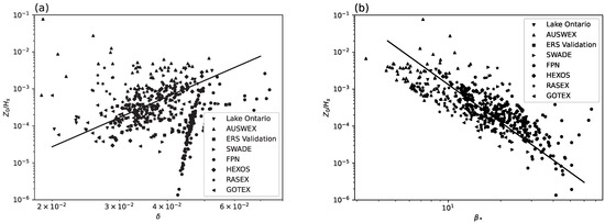
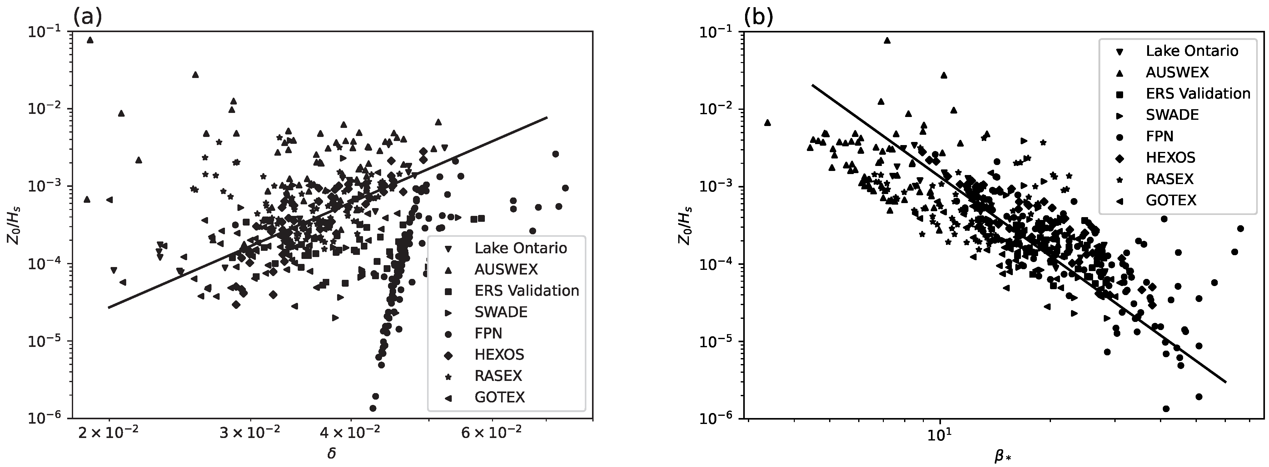
The dimensionless roughness $z_0/H_s$ of data points from eight datasets are plotted in Figure 1a against wave steepness $\delta$, the curve of TY01 is also shown as the solid line. It is shown that TY01 is able to describe the positive correlation between $z_0/H_s$ and $\delta$ in general, but the data points are quite scattered.

Figure 1. Dimensionless roughness $z_0/H_s$ vs. (a) wave steepness $\delta$ and (b) wave age ${\beta }_{*}$ for data points from eight datasets. The solid lines represent the curves of TY01 and DN03 in (a,b), respectively.

For comparison, we plot the same data points using the wave age scaling in Figure 1b, i.e., $z_0/H_s$ versus ${\beta }_{*}$. The curve of DN03 provides a better prediction of the dimensionless roughness $z_0/H_s$ than TY01, the data points are more concentrated near the curve than in Figure 1a.

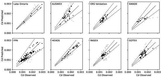
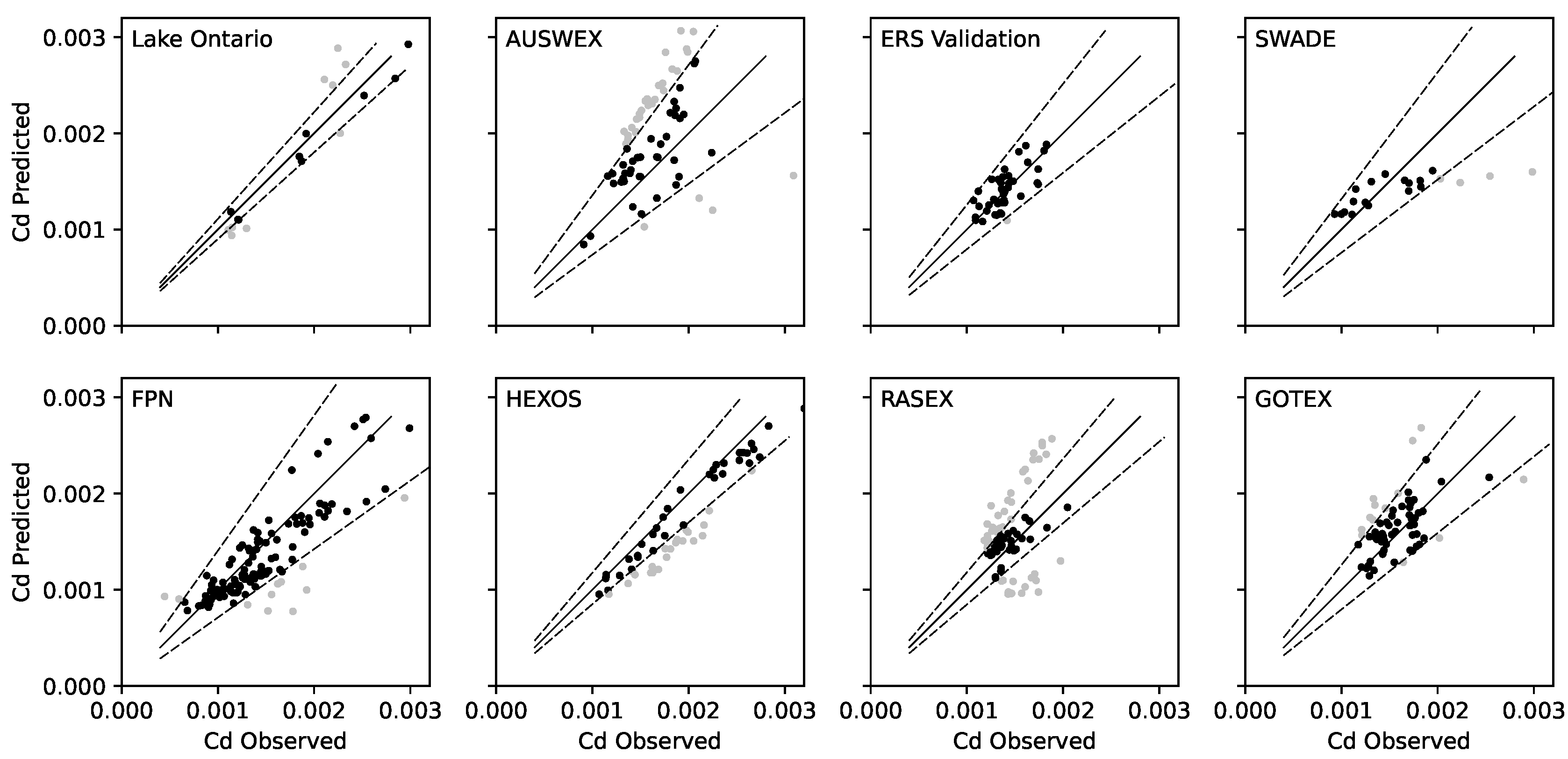
Although the plots of dimensionless roughness $z_0/H_s$ for all data points show the overall performance of two parameterizations, it is more instructive to test how they predict the drag coefficient. $z_0$ can be converted to $C_d$ by Equation (3). A comparison between measured and predicted $C_d$ has been made for each dataset, and the results of TY01 and DN03 are presented in Figure 2 and Figure 3, respectively. Note that the data points that fall within the 90% confidence regions are denoted as black points.

Figure 2. Measured drag coefficient vs. the value predicted by TY01 for eight datasets. Data points fall within the 90% confidence regions are shown in black points, and data points falling outside the 90% confidence regions are shown in grey points. Solid lines indicate the best fit between observations and predictions. Dashed lines represent the upper and lower boundaries of the 90% confidence regions.

Figure 3. Measured drag coefficient vs. the value predicted by DN03 for eight datasets. Data points fall within the 90% confidence regions are shown in black points, and data points fall outside the 90% confidence regions are shown in grey points. Solid lines indicate the best fit between observations and predictions. Dashed lines represent the upper and lower boundaries of the 90% confidence regions.

The 90% confidence regions for datasets using the EC method are calculated based on the sampling errors $\epsilon$ [69], where the sampling errors of six EC datasets can be calculated following Donelan [70]:

$$\epsilon =9.2z^{1/2}{(U{\rm Y})}^{-1/2},$$

(16)

where ${\rm Y}$ is the sampling time (s), U is the mean wind speed for an experiment, and z is the height of the anemometer above the water level. The sampling errors of eight datasets are summarized in Table 3. It is worth mentioning that the wind stress in the ERS Validation dataset was calculated using the ID method, Equation (16) is not applicable, and, following Drennan et al. [52], we assume an error equal to the mean sampling error of the EC data (25.77%). Similarly, data from GOTEX were collected from the aircraft, and the measuring instrument and post-processing method were inconsistent from other datasets. Equation (16) is suitable mainly for traditional platforms, i.e., buoy and tower. Thus, the sampling error for GOTEX dataset was also assumed as the mean sampling error for the EC data (25.77%).

Table 3. Sampling errors of eight datasets.

Dataset	Height (m)	Mean Wind Speed (m/s)	Sampling Time (s)	Number of Data	Sampling Error
Lake Ontario	7.8	11.39	4800	18	10.99%
AUSWEX	10	11.15	600	71	35.57%
ERS Validation	-	-	-	41	25.77%
SWADE	12	9.90	1020	20	31.71%
FPN	33	9.43	1800	116	40.57%
HEXOS	6	13.56	1200	58	17.67%
RASEX	7	10.05	1800	80	18.10%
GOTEX	-	-	-	67	25.77%

The sampling errors of the ERS validation dataset and the GOTEX dataset were assumed as the mean sampling error of six other datasets.

In Figure 2 and Figure 3, the 90% confidence regions are shown as the areas between the dotted lines, and the slope of the upper and the lower boundary line is $1+\epsilon$ and $1/(1+\epsilon )$, respectively. To evaluate the performance of TY01 and DN03 quantitatively, $P_{90}$ was defined as the percentage of data points that fall within the 90% confidence regions. The normalized bias ($NB$) is defined as:

$$NB=\frac{\sum (X_{mod}-X_{obs})}{\sum X_{obs}},$$

(17)

and the normalized root-mean-square-error ($NRMSE$) is defined as:

$$NRMSE=\sqrt{\frac{\sum {(X_{obs}-X_{mod})}^2}{\sum X_{obs}^2}},$$

(18)

where $X_{obs}$ is the observation, and $X_{mod}$ is the corresponding value calculated from parameterization schemes [71]. In addition, $P_{90}$, $NB$, and $NRMSE$ predicted by TY01 and DN03 for each dataset are shown in Table 4, also shown are the mean $\beta$, mean ${\beta }_{*}$, and mean $\delta$ for each dataset. From Table 4, we can see that the correlation between $P_{90}$ and $NB$ or $NRMSE$ is strong, and datasets with larger $P_{90}$ tend to have smaller $NB$ and $NRMSE$, and datasets in which TY01 performs better under $P_{90}$ are consistent with that under $NRMSE$. Considering that $P_{90}$ is consistent with $NB$ and $NRMSE$ qualitatively, and has the advantage of being able to take into account the sampling error of each dataset, we mainly focus on $P_{90}$ in the following analysis.

Table 4. $P_{90}$, $NB$, and $NRMSE$ predicted by TY01 and DN03 for each dataset.

Dataset	Mean $\mathit{\beta }$	Mean ${\mathit{\beta }}_{*}$	Mean $\mathit{\delta }$	${\mathit{P}}_{90}$-TY01	${\mathit{P}}_{90}$-DN03
Lake Ontario	0.6542	16.69	0.0354	0.5000	0.5000
AUSWEX	0.2978	7.54	0.0367	0.6620	0.5493
ERS Validation	0.7984	20.89	0.0392	0.3171	0.9756
SWADE	0.7487	18.88	0.0405	0.4000	0.8000
FPN	0.9917	27.43	0.0481	0.1638	0.9052
HEXOS	0.8007	19.20	0.0362	0.7931	0.6379
RASEX	0.4798	12.68	0.0352	0.6875	0.4625
GOTEX	0.6977	17.69	0.0329	0.8507	0.8060
Total	0.6948	18.18	0.0390	0.5393	0.7155
Dataset	NB-TY01	NB-DN03	NRMSE-TY01	NRMSE-DN03
Lake Ontario	−0.0847	−0.0003	0.1330	0.1346
AUSWEX	−0.2587	0.2120	0.3447	0.3734
ERS Validation	0.3727	0.0059	0.4377	0.1101
SWADE	0.1514	−0.1241	0.3990	0.2796
FPN	0.6924	−0.0938	0.7757	0.1985
HEXOS	−0.0107	−0.1125	0.1089	0.1358
RASEX	−0.0828	0.0790	0.1931	0.2603
GOTEX	0.0684	0.0517	0.1839	0.1857
Total	0.1464	0.0090	0.4327	0.2302

Schemes with better performance under different indicators are bolded.

We first consider the results predicted by TY01 shown in Figure 2 and Table 4. TY01 is seen to work well for the AUSWEX, HEXOS, RASEX, and GOTEX datasets with a $P_{90}$ larger than 0.65, but $C_d$ measured in ERA Validation, SWADE, and FPN datasets was poorly predicted with a $P_{90}$ less than 0.4, especially in the FPN dataset ($P_{90}=0.1638$). As we can see from Figure 2, $C_d$ in ERS Validation and FPN datasets were extremely overpredicted by TY01, it is worth noticing that the mean ${\beta }_{*}$ of ERS Validation and FPN datasets were the largest two among eight datasets (both larger than 20), corresponding to a mature wave field. Moreover, TY01 underpredicted $C_d$ from AUSWEX and RASEX datasets, whose mean ${\beta }_{*}$ was the smallest two among eight datasets. The performance of TY01 shows an obvious sensitivity to ${\beta }_{*}$; for datasets having a larger ${\beta }_{*}$, TY01 tend to overpredict $C_d$ from them; but, for datasets having a smaller ${\beta }_{*}$, $C_d$ from them was underpredicted.

The results of DN03 were shown in Figure 3 and Table 4. The overall performance of DN03 is better than TY01. The results of DN03 from ERS Validation, SWADE, and FPN datasets are much better than TY01, but $C_d$ measured in AUSWEX, HEXOS, and RASEX was poorly predicted and worse than TY01. For datasets in which DN03 performs well, the mean ${\beta }_{*}$ was seen to be large (20.89, 18.88, 27.43, and 17.69 for ERS Validation, SWADE, FPN, and GOTEX, respectively), and in two datasets that have a smaller ${\beta }_{*}$ (7.54 for AUSWEX and 12.68 for RASEX), the performance of DN03 is quite worse. Therefore, the performance of DN03 also shows a sensitivity to ${\beta }_{*}$.

In order to analyze the applicability of TY01 and DN03 in different conditions, we examine the sensitivity of their performance to $\beta$, ${\beta }_{*}$, and $\delta$. Here, we use TY01_in to denote the data points predicted by TY01 that fall within the 90% confidence regions, corresponding to those data accurately predicted by TY01; and TY01_out to denote the data points predicted by TY01 that fall outside the 90% confidence regions, corresponding to those data that are not accurately predicted by TY01. DN03_in and DN03_out are the same, but for data points predicted by DN03. Table 5 shows the mean $\beta$, mean ${\beta }_{*}$, and mean $\delta$ of TY01_in, TY01_out, DN03_in, and DN03_out.

Table 5. Sensitivities of the performance of TY01 and DN03 to $\beta$, ${\beta }_{*}$, and $\delta$.

	Mean $\mathit{\beta }$	Mean ${\mathit{\beta }}_{*}$	Mean $\mathit{\delta }$
TY01_in	0.5873	14.60	0.0369
TY01_out	0.8206	22.38	0.0414
DN03_in	0.7205	19.08	0.0398
DN03_out	0.6302	15.93	0.0369

The mean $\beta$ and ${\beta }_{*}$ of TY01_in is much smaller than that of TY01_out, demonstrating that TY01 tends to have better performance at younger wave conditions. The mean $\delta$ of TY01_in is close to the mean $\delta$ of TY01_out, indicating that the performance of TY01 is not sensitive to $\delta$. The difference of the mean $\beta$ between DN03_in and DN03_out is not as obvious as between TY01_in and TY01_out, but the difference of the mean ${\beta }_{*}$ between DN03_in and DN03_out is non-negligible. The difference of the mean $\delta$ between DN03_in and DN03_out is not obvious, demonstrating that the performance of DN03 is also not sensitive to the wave steepness.

Considering that the performance of TY01 and DN03 is both sensitive to ${\beta }_{*}$, to further investigate the sensitivities of the performance of TY01 and DN03 to ${\beta }_{*}$, we divide the 471 data from eight datasets into 10 groups of roughly equal numbers (47 or 48 per group) according to ${\beta }_{*}$ from low to high, and calculate the $P_{90}$ of each group, the results are shown in Table 6. Changes in performance of TY01 and DN03 with ${\beta }_{*}$ are clearly demonstrated, when ${\beta }_{*}$ exceeds 16, the performance of TY01 drops significantly; when ${\beta }_{*}$ is smaller than 10, the performance of DN03 is relatively poor. Considering the different performance of TY01 and DN03 in different conditions, it is reasonable to combine them by using TY01 in small ${\beta }_{*}$ conditions and using DN03 in large ${\beta }_{*}$ conditions. Another issue is the choice of the demarcation point between TY01 and DN03, since the datasets used in this study do not cover all wind and wave conditions, and there are inconsistencies between datasets due to different observation and processing methods, we cannot determine the demarcation points arbitrarily as the point where the performance of DN03 exceeds TY01. Therefore, we use the $\delta -{\beta }_{*}$ relationship derived from Toba’s [72] 3/2 power law to determine the demarcation points between TY01 and DN03. The well-known 3/2 power law is given as:

$$H_{*}=B{T}_{*}^{3/2},$$

(19)

where $H_{*}=g{H}_s/u_{*}^2$ and $T_{*}=g{T}_s/u_{*}$ are non-dimensional significant wave height and period, and $B=0.062$ is a constant. The 3/2 power law has been verified by many studies [64,73,74], which is suitable for low to extreme wind conditions [48]. Multiplying Equation (19) by $2\pi u_{*}^2/g^2{T}_p^2$, we get:

$$\frac{2\pi H_s}{g{T}_p^2}=2\pi \times 0.062{(\frac{g{T}_p^4}{u_{*}{T}_s^3})}^{-1/2},$$

(20)

by using the relation between significant wave period $T_s$ and peak wave period $T_p$ [75,76]:

$$T_s=0.91T_p,$$

(21)

and by calling the relation $c_p=g{T}_p/2\pi$, Equation (20) can be rewritten as:

$$\delta =0.135{\beta }_{*}^{-1/2}.$$

(22)

Table 6. $P_{90}$ of 10 groups divided according to ${\beta }_{*}$ from low to high.

Groups with Different ${\mathit{\beta }}_{*}$ Ranges	${\mathit{P}}_{90}$-TY01	${\mathit{P}}_{90}$-DN03
Group 1 ($3.38\le {\beta }_{*}\le 7.24$)	0.7083	0.3125
Group 2 ($7.26\le {\beta }_{*}\le 9.95$)	0.7021	0.6170
Group 3 ($10.02\le {\beta }_{*}\le 12.54$)	0.6596	0.6596
Group 4 ($12.59\le {\beta }_{*}\le 13.75$)	0.7447	0.8085
Group 5 ($13.78\le {\beta }_{*}\le 16.12$)	0.6809	0.8298
Group 6 ($16.13\le {\beta }_{*}\le 18.36$)	0.5106	0.8085
Group 7 ($18.43\le {\beta }_{*}\le 20.78$)	0.4894	0.7447
Group 8 ($20.79\le {\beta }_{*}\le 25.59$)	0.4894	0.8085
Group 9 ($25.70\le {\beta }_{*}\le 31.33$)	0.4043	0.7872
Group 10 ($31.40\le {\beta }_{*}\le 66.10$)	0.0000	0.7660

Schemes with better performance are bolded.

By combining Equation (7) (function of DN03), Equation (9) (function of TY01), and Equation (22), we work out that the curves of TY01 and DN03 intersect at ${\beta }_{*}=15.21$. According to the above inference, ${\beta }_{*}=15.21$ is selected as the demarcation point between TY01 and DN03, TY01 is adopted when ${\beta }_{*}<15.21$, and DN03 is adopted when ${\beta }_{*}\ge 15.21$:

$$z_0/H_s=\left\{\begin{array}{cc}1.2\times {10}^2{\delta }^{4.5},\hfill & {\beta }_{*}<15.21\hfill \\ 3.35\times {\beta }_{*}^{-3.4},\hfill & {\beta }_{*}\ge 15.21\hfill \end{array}.\right.$$

(23)

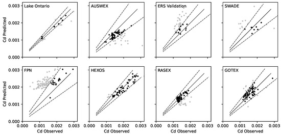
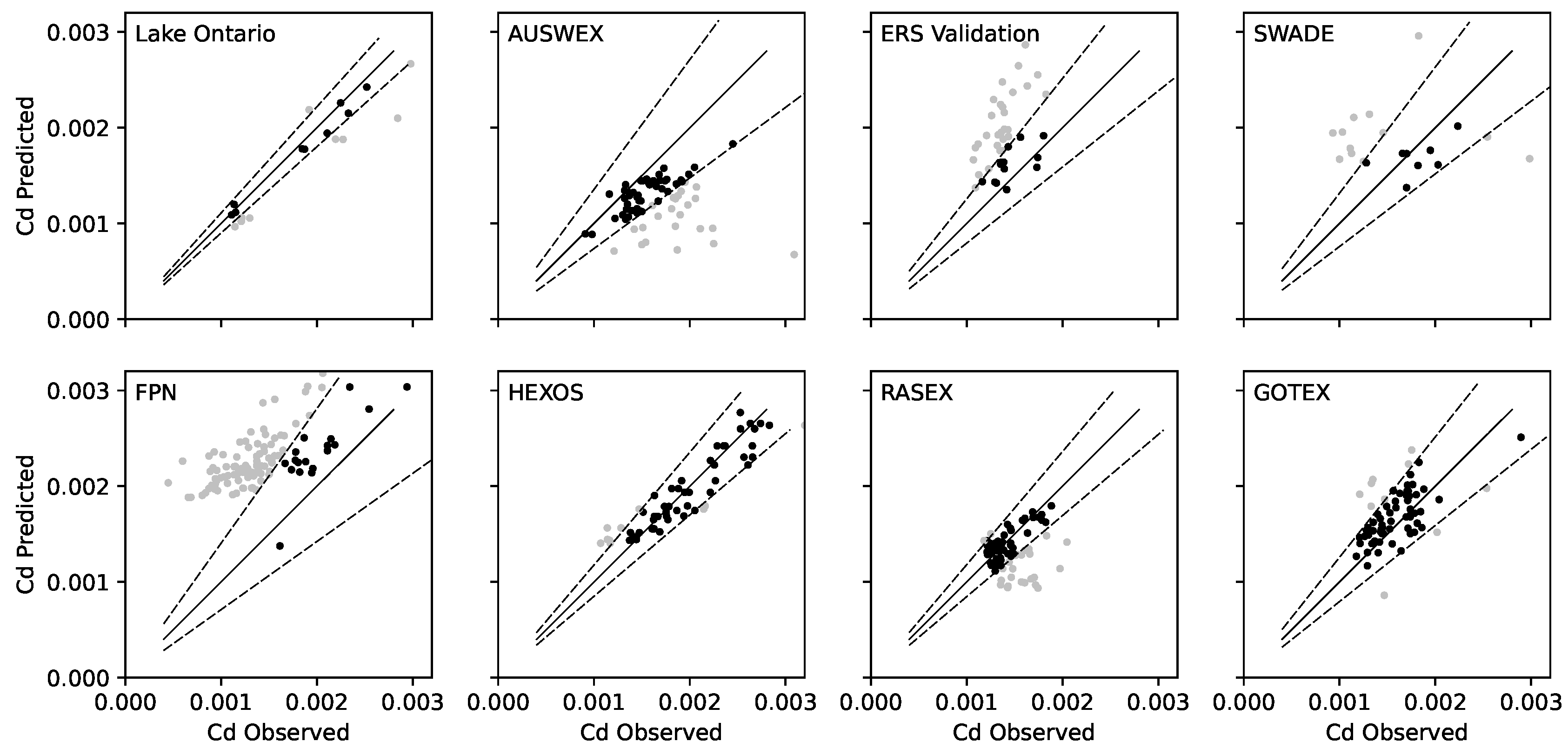
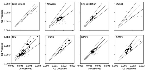
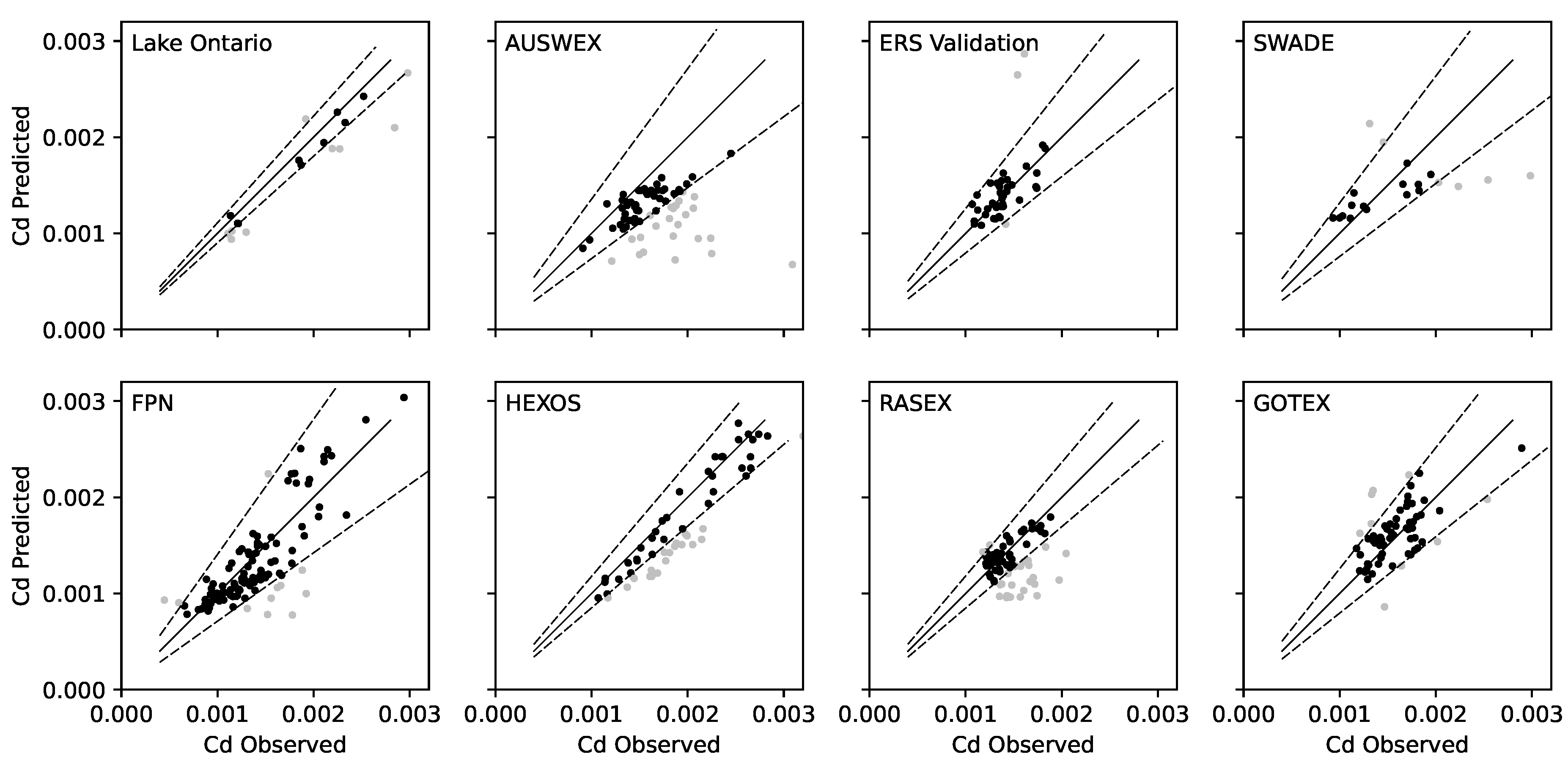
To verify the validity of the combination of TY01 and DN03 given in Equation (23), Figure 4 plotted a comparison between the measured $C_d$ and the corresponding values predicted by Equation (23) as in Figure 2 and Figure 3. By comparing Figure 2 and Figure 4, we can see that the performance of the combined scheme is much better than that of TY01, especially in ERS Validation and FPN datasets. By comparing Figure 3 and Figure 4, the improvement of the combined scheme compared to DN03 mainly comes from the RASEX dataset; most of the RASEX data overestimated by DN03 have been improved in the combined scheme. We further compared the $P_{90}$, $NB$, and $NRMSE$ predicted by TY01, DN03, and the combined scheme for the total eight datasets (Table 7); the results show that the performance of the combined scheme is much better than TY01 in $P_{90}$ and $NRMSE$, and slightly better than that of DN03, $NB$ predicted by the combined scheme is slightly worse than DN03. Considering that $NB$ mainly describes the overestimation or underestimation of the prediction, and can be offset if both overestimation and underestimation exist, while $P_{90}$ and $NRMSE$ are the key parameters to show the overall performance; the results in Table 7 prove that the performance of the combined scheme is better than TY01 and DN03.

Figure 4. Measured drag coefficient vs. the value predicted by Equation (23) for eight datasets. Data points fall within the 90% confidence regions are shown in black points, and data points fall outside the 90% confidence regions are shown in grey points. Solid lines indicate the best fit between observations and predictions. Dashed lines represent the upper and lower boundaries of the 90% confidence regions.

Table 7. $P_{90}$, $NB$, and $NRMSE$ predicted by TY01, DN03, and the combined scheme (Equation (23)) for the total eight datasets.

	TY01	DN03	Combined
$P_{90}$	0.5393	0.7155	0.7537
$NB$	0.1464	0.0090	0.0496
$NRMSE$	0.4327	0.2302	0.2249

Schemes with better performance are bolded.

4. Effect of Sea Foam

TY01 was developed using three datasets: HEXOS, RASEX, and Lake Ontario, and DN03 was developed using the pure wind sea subsets of five datasets: AGILE (measured from the 15-m research vessel AGILE) [77], FETCH (Flux, sea state and remote sensing in conditions of variable fetch) [78], HEXOS, SWADE, and WAVES (Water–Air Vertical Exchange Study) [79]; these datasets were collected under low and moderate wind conditions ($U_{10}\le 20$ m/s). Compared to low and moderate wind conditions, a significant change in high wind conditions ($U_{10}\ge 25$ m/s) is the generation of sea foam due to intense wave breaking, which plays an important role in the leveling off or decrease of $C_d$ and $z_0$. Since the effect of sea foam on sea surface roughness is minimal at low to moderate wind speeds [38,55], the effect of sea foam was not implicitly included in the proposing of TY01 and DN03, and an introduction of the effect of sea foam to TY01 and DN03 will enhance their applicability for high wind speed conditions.

A semi-empirical model is proposed by [55] to estimate the influence of sea foam on aerodynamic roughness. Their model treats the effective air–sea aerodynamic roughness ($z_{eff}$) as the weighted sum of two parts: one is the foam-free ($z_n$) part and the other is the foam-covered ($z_f$) part. The average $z_{eff}$ under area S is assumed as follows:

$$z_{eff}=\frac{1}{S}({\int }_{S_n}{z}_{n}d{S}^{\prime }+{\int }_{S_f}{z}_{f}d{S}^{\prime }).$$

(24)

Here, $S=S_n+S_f$ is the total area, in which $S_n$ and $S_f$ are the foam-free and foam-cover areas, respectively. Thus, Equation (24) can be rewritten as:

$$z_{eff}=\frac{S-S_f}{S}{z}_n+\frac{S_f}{S}{z}_f,$$

(25)

by defining ${\alpha }_f=S_f/S$ as the fractional foam coverage, we obtain:

$$z_{eff}=(1-{\alpha }_f)z_n+{\alpha }_f{z}_f.$$

(26)

The fractional foam coverage ${\alpha }_f$ is highly related to $U_{10}$ [80]. The function between ${\alpha }_f$ and $U_{10}$ can be approximated from the observational data as in Holthuijsen et al. [80]:

$${\alpha }_f=\gamma \tanh [\alpha \exp (\zeta U_{10})],$$

(27)

with $\alpha =0.00255$, $\zeta =0.166$, and $\gamma =0.98$. To demonstrate the different patterns of ${\alpha }_f$ in different situations, a universal dimensionless form of Equation (27) is given as:

$${\alpha }_f=\gamma \tanh [\alpha \exp (\tilde{\zeta }\frac{U_{10}}{U_{10}^{(s)}})],$$

(28)

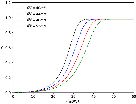
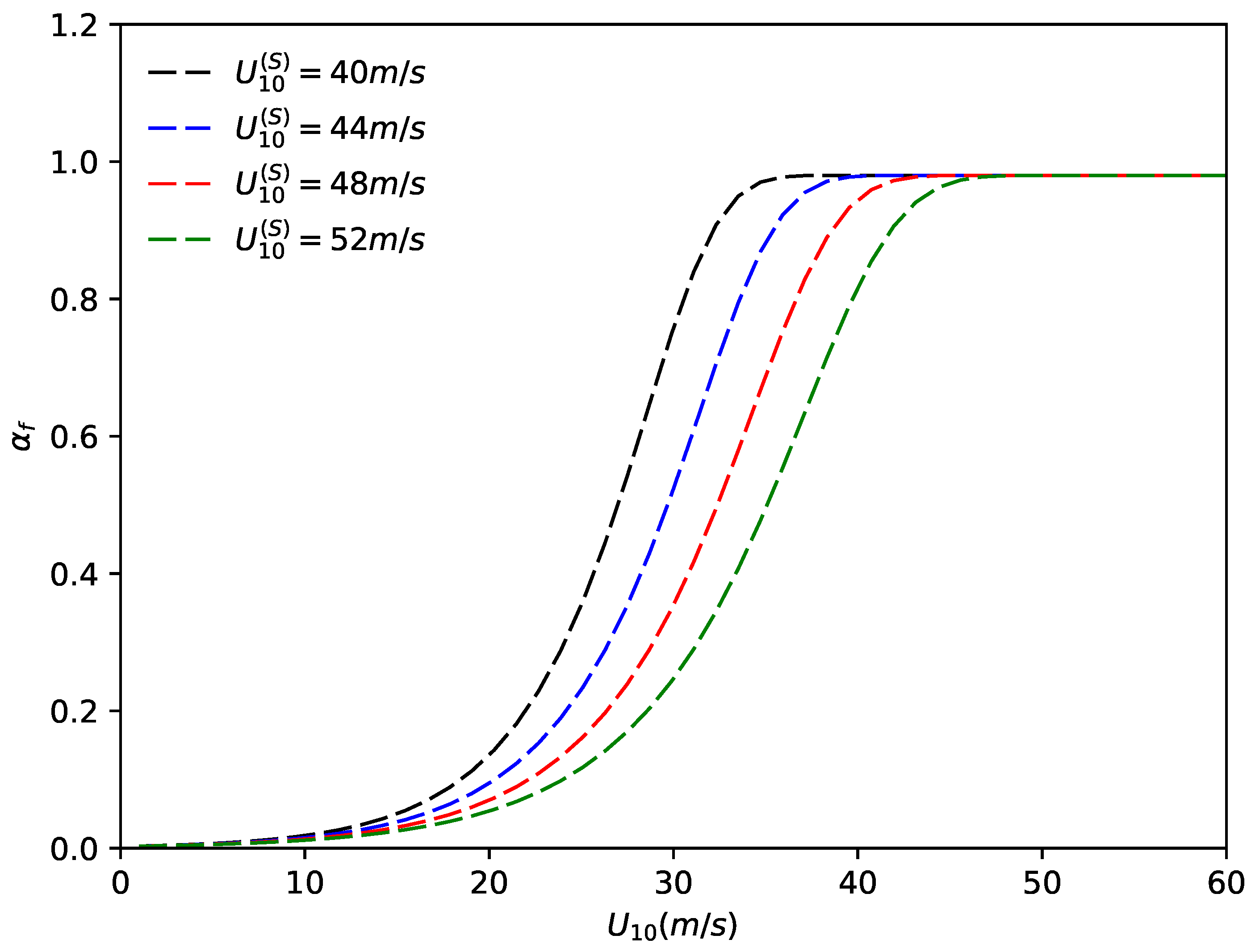
where $\tilde{\zeta }=8$, $U_{10}^{(S)}$ is the saturation speed, defined as the value where the difference between ${\alpha }_f$ and its saturation limit ${\alpha }_f=1$ is less than 2%. The curve of foam coverage ${\alpha }_f$ versus $U_{10}$ from Equation (28) varies and $U_{10}^{(S)}$ is presented in Figure 5, the results show that, when the wind speed $U_{10}$ exceeds 40 m/s, the foam coverage ${\alpha }_f$ is very close to 0.98, while ${\alpha }_f$ is minimal when $U_{10}$ is less than 20 m/s. Observational data collected from the open ocean by Holthuijsen et al. [80] suggest a value of $U_{10}^{(S)}=48$ m/s. According to the open-ocean experimental data for $C_d$ or, alternatively, $z_{eff}$ [29], it is assumed that the minimum value for $C_d=0.0017$ or, $z_{eff}=0.0003$ m is reached at the same wind speed $U_{10}=48$ m/s (see Figure 2 and Figure 3 in Golbraikh and Shtemler [55]). Because the relation between $C_d$ and $U_{10}$ in laboratory conditions is quite different from that of the open ocean, Golbraikh and Shtemler [55] suggested a different minimum value for $z_{eff}$ in laboratory conditions, which is $z_{eff}=0.0028$ m. Then, we adopt $U_{10}=48$ m/s as the saturation velocity, and the minimum value of $z_{eff}=0.0003$ m as the foam-covered aerodynamic roughness $z_f$ in Equation (26) for open ocean conditions, and the minimum value of $z_{eff}=0.0028$ m for laboratory conditions. As the effect of sea foam was not implicitly included in the proposing of TY01 and DN03, the aerodynamic roughness predicted by Equation (23) can be taken as the foam-free aerodynamic roughness $z_n$ in Equation (26), substituting Equation (23) into Equation (26), a new parameterization of sea surface roughness including the impact of sea foam is obtained:

$$z_0/H_s=\left\{\begin{array}{cc}(1-{\alpha }_f)1.2\times {10}^2{\delta }^{4.5}+{\alpha }_f{z}_f/H_s,\hfill & {\beta }_{*}<15.21\hfill \\ (1-{\alpha }_f)3.35\times {\beta }_{*}^{-3.4}+{\alpha }_f{z}_f/H_s,\hfill & {\beta }_{*}\ge 15.21\hfill \end{array},\right.$$

(29)

where $z_0$ is the aerodynamic roughness, $\delta$ is wave steepness, ${\beta }_{*}$ is wave age, $H_s$ is the significant wave height, ${\alpha }_f$ is the foam coverage (calculated from Equation (28)), and $z_f$ is the foam-covered aerodynamic roughness (taken as 0.0003 m for open ocean conditions, and 0.0028 m for laboratory conditions in this study). By combining TY01 and DN03 in the form of a piecewise function, the new proposed parameterization is able to make better predictions of $z_0$ in various wind and wave conditions. By adding the impact of sea foam, the predictions of $z_0$ in high wind speed conditions are improved.

Figure 5. The foam coverage ${\alpha }_f$ versus $U_{10}$ from Equation (28) in different $U_{10}^{(S)}$.

5. Validation and Discussion

As aforementioned, the proposed parameterization calls TY01 and DN03 according to different wave ages; its comparison against observations in low and moderate wind conditions have been made in Section 3. In this section, we will make a brief validation on the behavior of $C_d$ predicted by the proposed parameterization under high wind speed conditions. Specifically, datasets from several recent experiments [27,28,29,68] with observations under high wind speed conditions are compared with the new parameterization.

5.1. Estimation of $H_s$

These observational data were presented in the form of $C_d$ vs. $U_{10}$, in order to compare the proposed parameterization with these observational data; it is essential to parameterize $H_s$ with $U_{10}$.

Several schemes were proposed for the parameterization of $H_s$. From the formulas for fully developed wave field in deep water, Taylor and Yelland [51] proposed a parameterization of $H_s$:

$$H_s=0.0248U_{10}^2.$$

(30)

According to Equation (30), Fairall et al. [81] developed an empirical formula for predicting $H_s$ in the Coupled Ocean-Atmosphere Response Experiment bulk algorithm (COARE 3.0):

$$H_s=0.018U_{10}^2(1+0.015U_{10}).$$

(31)

In addition, using 15 years of hourly buoy data, Wang et al. [82] developed a $H_s$ scheme for open oceans:

$$H_s=0.0143U_{10}^2+0.9626.$$

(32)

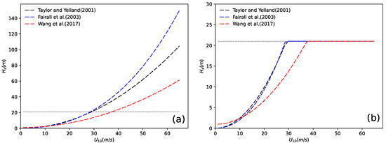
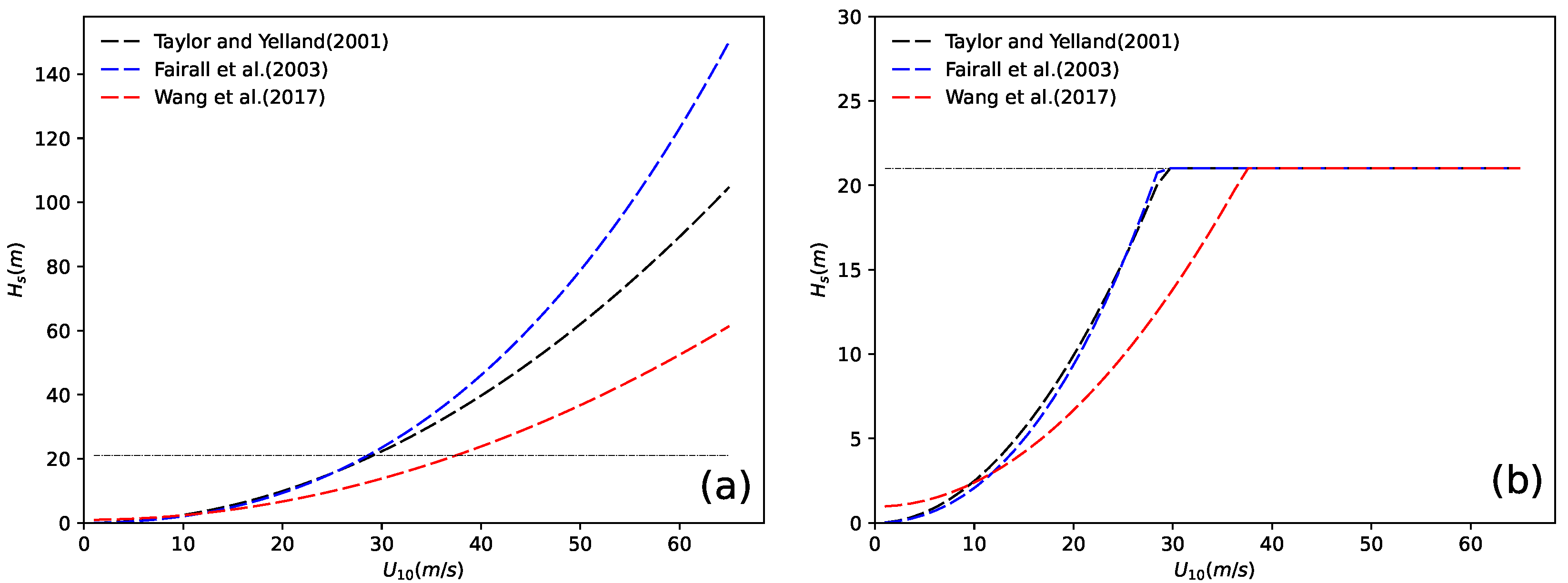
These schemes all reveal the monotonically increasing of $H_s$ with $U_{10}$, and this trend has been verified in low and moderate wind speeds, their applicability in high wind speed conditions is doubtful. The plots of $H_s$ versus $U_{10}$ of the three schemes above are shown in Figure 6a, the values of $H_s$ from three schemes are relatively reasonable at low and moderate wind speeds; however, as the wind speed increases, $H_s$ becomes unreasonably large, the values of $H_s$ calculated from three schemes all exceed 50 m at $U_{10}=60$ m/s, which are obviously unreasonable. However, accurate prediction of $H_s$ under high wind speeds requires the help of numerical models. Considering that our purpose is only to get the brief relationship between $H_s$ and $U_{10}$, we simply add a threshold of 21 m to $H_s$ to replace the unreasonably large value under high wind speeds (Figure 6b). The value of 21 m comes from the largest $H_s$ measured by the radar altimeter onboard the Jason 2 satellite (http://cersat.ifremer.fr/user-community/news/item/346-record-breaking-wave-heights-and-periods-in-the-north-atlantic, accessed on 11 February 2021) which is 20.1 m; here, we round it to 21 m.

Figure 6. $H_s$ versus $U_{10}$ (a) without threshold and (b) with threshold from Taylor and Yelland [51], Fairall et al. [81], and Wang et al. [82]. The threshold of $H_s$ = 21 m is shown as the thin dashed line.

5.2. Validation of the Proposed Parameterization

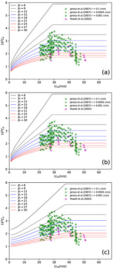
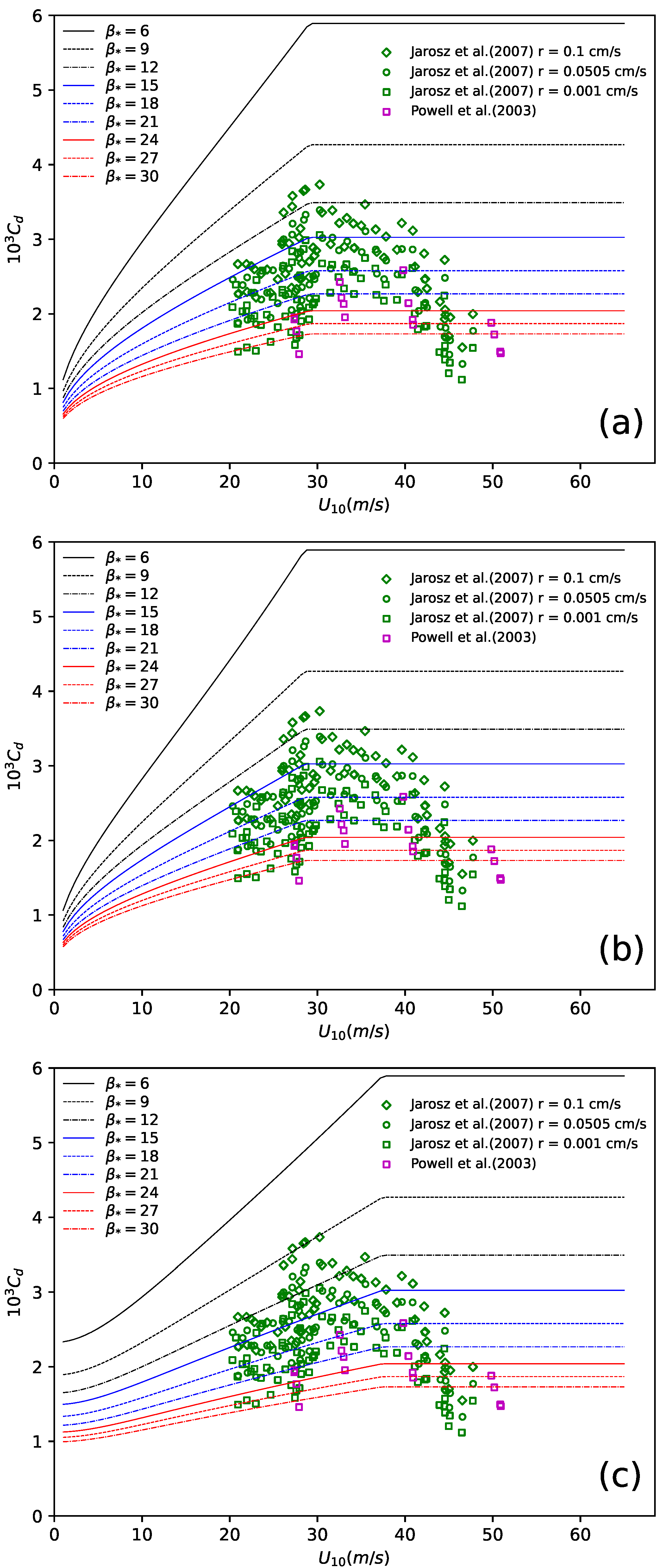
In order to show how sea foam affects our results, the comparison between the curves of our parameterization without the effect of sea foam (Equation (23)) and the field observations from Powell et al. [29] and Jarosz et al. [68] is presented in Figure 7. Figure 7a–c denotes the different relations from $H_s$ estimated from Taylor and Yelland [51], Fairall et al. [81], and Wang et al. [82], respectively. For the curves of ${\beta }_{*}<15.21$, $\delta$ has been converted to ${\beta }_{*}$ using the $\delta -{\beta }_{*}$ relationship derived from Toba’s [72] 3/2 power law (Equation (22)). From Figure 7, we can see that the curves of $C_d$ from Equation (23) can not reproduce the decreasing of $C_d$ at high winds. The effect of sea foam can be seen from the comparison between Figure 7 and Figure 8.

Figure 7. Comparison between $C_d$ predicted by the new parameterization without the effect of sea foam (Equation (23)) under different wave ages using $H_s$ estimated from (a) Taylor and Yelland [51]; (b) Fairall et al. [81]; and (c) Wang et al. [82] and the field observations.

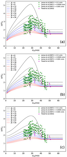
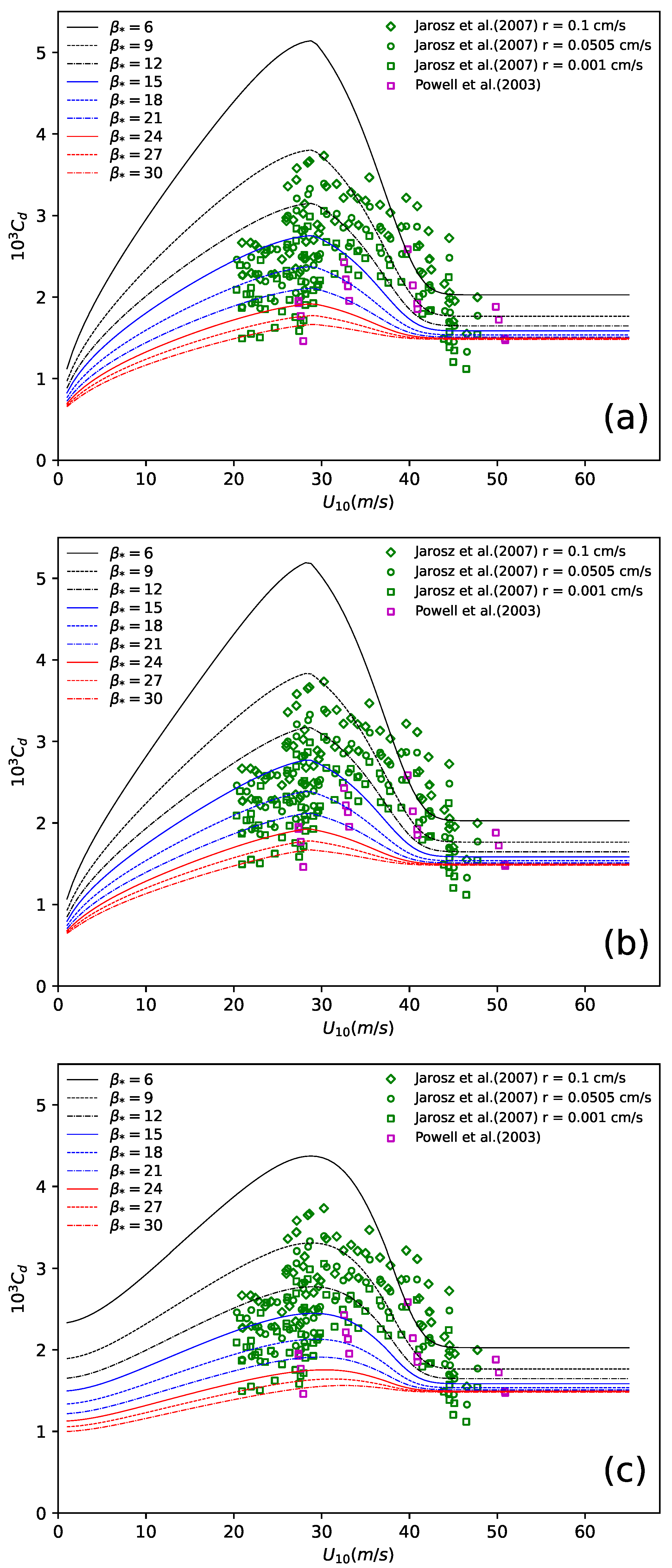
Figure 8. Comparison between $C_d$ predicted by the new parameterization with the effect of sea foam (Equation (29)) under different wave ages using $H_s$ estimated from (a) Taylor and Yelland [51]; (b) Fairall et al. [81]; and (c) Wang et al. [82] and the field observations.

Given that $z_f$ in Equation (29) is taken as different values for field and laboratory conditions, we compared the new parameterization with field and laboratory observations separately. Figure 8 shows the comparison between $C_d$ predicted by the new parameterization (Equation (29)) under different wave ages and the field observations from Powell et al. [29] and Jarosz et al. [68]. From Figure 8, we can see that $C_d$ predicted by the new proposed parameterization using different $H_s$ schemes are generally consistent. $C_d$ increases with wind speed in the range of 0–30 m/s, the maximum values are reached at about 30∼35 m/s, then decreases at the wind speed about 35∼45 m/s under the effect of sea foam, for wind speed larger than 45 m/s, the values of $C_d$ do not change much. By comparing Figure 7 and Figure 8, the effect of sea foam is obvious, by adding the sea foam, our parameterization can reproduce the reduction of $C_d$ at $U_{10}$ > 30 m/s, which is closer to the observations.

Results from $H_s$ schemes proposed by Taylor and Yelland [51] and Fairall et al. [81] (Figure 8a,b, respectively) do not show much differences, but the results from Wang et al. [82] (Figure 8c) are different from the other at low and moderate wind speeds, in which the values of $C_d$ are larger than the other two, especially for the younger wave. The difference is caused by the intercept of the formula proposed by Wang et al. [82] (see Equation (32)), when $U_{10}$ is close to zero, $H_s$ still has an initial value, given that young wave fields generally do not correspond to low wind speeds; this difference is not obvious in practice.

The curves of the new proposed parameterization shown in Figure 8 can cover the range of the field observational data well, and the scatter of the observations can be explained as the effect of wave state. The reduction of $C_d$ under high wind speeds is successfully reproduced by the new proposed parameterization, $C_d$ predicted by the new proposed parameterization reach the maximum values in the wind range of 30∼35 m/s, which is consistent with the field measurements in Jarosz et al. [68] and Powell et al. [29]. The maximum value in Jarosz et al. [68] with the resistance coefficient of 0.1 cm/s (∼$3.7\times {10}^{-3}$) is close to the maximum value of ${\beta }_{*}=9$ in Figure 8a,b, and is between ${\beta }_{*}=9$ and ${\beta }_{*}=6$ in Figure 8c. Furthermore, compared with the curves in Jarosz et al. [68] (cf Figure 2 and Figure 3 therein), our parameterization provides $C_d$ values for $U_{10}$ > 50 m/s, while curves in Jarosz et al. [68] did not, considering that conditions with $U_{10}$ larger than 50 m/s are common in tropical cyclones, our parameterization is suitable for the usage in tropical cyclone modeling and storm surge modeling. Since the simultaneous wave state was not measured by Jarosz et al. [68], we cannot compare the predictions of $C_d$ with the observations directly.

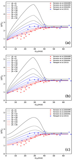
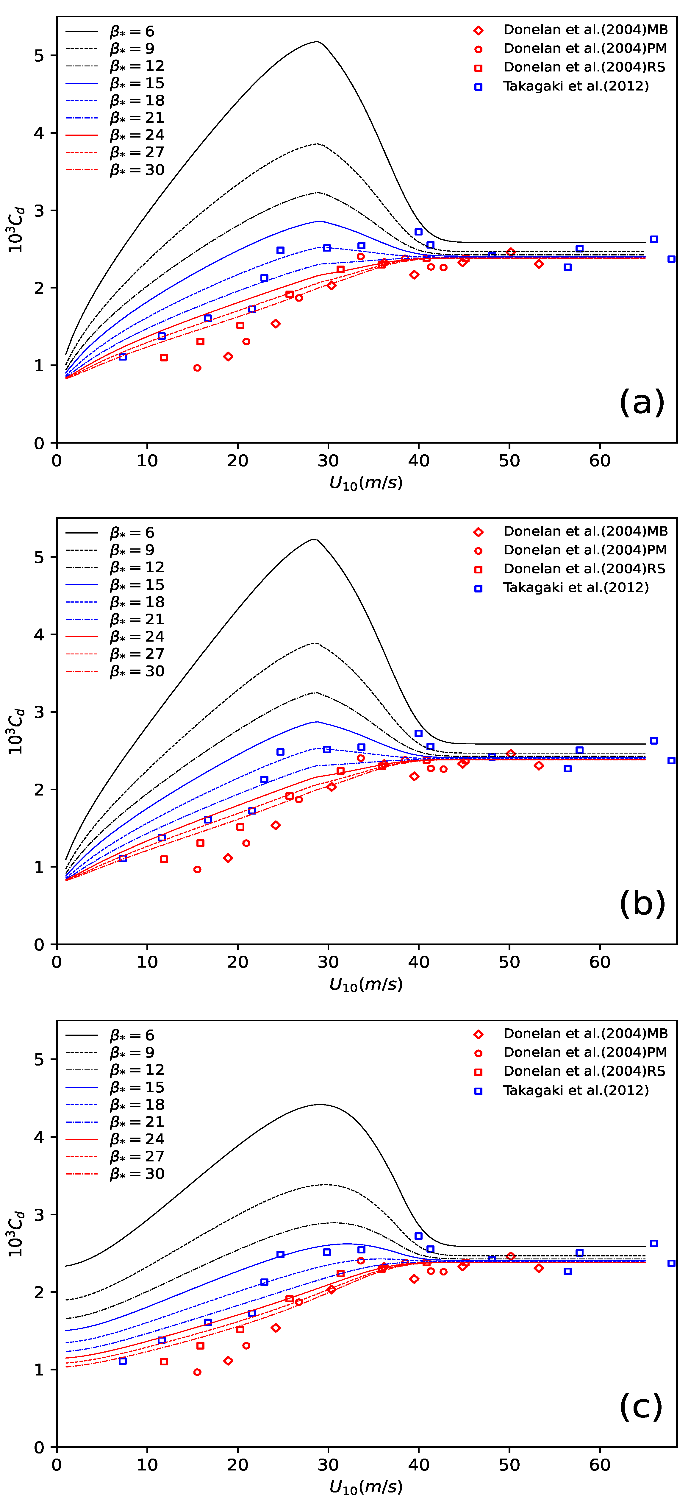
Figure 9 shows the comparison between $C_d$ predicted by the new parameterization under different wave ages and the laboratory observations from Donelan et al. [27] and Takagaki et al. [28]. The laboratory measurements do not show a decreasing trend under high wind speeds, their $C_d$ tend to saturate at wind speeds larger than 35 m/s. The difference between the field and laboratory measurements can be expected due to significant differences in fetch [35]; in addition, in hurricane conditions, the wave field is dominated by swell generated in the high wind areas, but it will not be reproduced under laboratory conditions [83]. Consistent with the laboratory measurements, $C_d$ predicted by the new parameterization also shows a saturation at $U_{10}>40$ m/s, the saturation values of the observations match the predicted $C_d$ well, both of them are very close to $C_d=0.0024$. For $U_{10}<30$ m/s, the values of observations concentrate near the curve of a larger wave age; considering that wave age is negative related to wind speed, and lower wind speed usually corresponds to a larger wave age, this result is reasonable. Observations from Donelan et al. [27] are slightly lower than that predicted by our parameterization, especially for MB and PM methods, this slightly difference is caused by the calculation method and the measuring instrument, i.e., the RS method uses the stress data directly measured from an x-film anemometer, the PM method uses wind speed data measured from the hot-film anemometry, and the MB method uses the bottom stress from DPIV and surface elevation from laser/line scan cameras to calculate $C_d$.

Figure 9. Comparison between $C_d$ predicted by the new parameterization under different wave ages using $H_s$ estimated from (a) Taylor and Yelland [51]; (b) Fairall et al. [81]; and (c) Wang et al. [82] and the laboratory observations.

Although the proposed parameterization can reasonably explain the behavior of the observational data, it should be pointed out that the values predicted by the new parameterization have not been compared with the observational data directly due to the lack of simultaneous wave state measurements under high wind speed conditions. Thus, more field and laboratory experiments containing simultaneous wind and wave state measurements are needed to further verify the performance of the new parameterization, and to investigate the mechanism of momentum transfer across the air–sea interface.

5.3. Comparison with Other Parameterizations

In this section, the performance of our parameterization has been compared with three different parameterizations, these parameterizations have been proposed for the calculation of $C_d$ in high wind speed conditions, and the saturation of $C_d$ has been dealt with different method.

Based on the work of Powell [84] and Garratt [17], Luettich and Westerink [85] offered a formulation that divides the tropical cyclone into three sectors and calculated $C_d$ accordingly; this formula has been used in the ADvanced CIRCulation (ADCIRC) storm surge model (here, we denote it as ADCIRC). For the right sector of a storm:

$$C_d=\left\{\begin{array}{cc}(0.75+0.067U_{10})\times {10}^{-3},\hfill & U_{10}\le 35\mathrm{m}/\mathrm{s}\hfill \\ 0.0020+\frac{(0.0030-0.0020)}{(45.0-35.0)}(U_{10}-35.0),\hfill & 35\mathrm{m}/\mathrm{s}\le U_{10}\le 45\mathrm{m}/\mathrm{s}\hfill \\ 0.0030,\hfill & U_{10}>45\mathrm{m}/\mathrm{s}\hfill \end{array},\right.$$

(33)

for the rear sector of a storm:

$$C_d=\left\{\begin{array}{cc}(0.75+0.067U_{10})\times {10}^{-3},\hfill & U_{10}\le 35\mathrm{m}/\mathrm{s}\hfill \\ 0.0020+\frac{(0.0010-0.0020)}{(45.0-35.0)}(U_{10}-35.0),\hfill & 35\mathrm{m}/\mathrm{s}\le U_{10}\le 45\mathrm{m}/\mathrm{s}\hfill \\ 0.0010,\hfill & U_{10}>45\mathrm{m}/\mathrm{s}\hfill \end{array},\right.$$

(34)

and for the left front sector of a storm:

$$C_d=\left\{\begin{array}{cc}0.0018,\hfill & U_{10}\le 25\mathrm{m}/\mathrm{s}\hfill \\ 0.0018+\frac{(0.0045-0.0018)}{(30.0-25.0)}(U_{10}-25.0),\hfill & 25\mathrm{m}/\mathrm{s}\le U_{10}\le 30\mathrm{m}/\mathrm{s}\hfill \\ 0.0045+\frac{(0.0010-0.0045)}{(45.0-30.0)}(U_{10}-35.0),\hfill & 30\mathrm{m}/\mathrm{s}\le U_{10}\le 45\mathrm{m}/\mathrm{s}\hfill \\ 0.0010,\hfill & U_{10}>45\mathrm{m}/\mathrm{s}\hfill \end{array}.\right.$$

(35)

Using more than 6000 near-surface flux measurements collected from low-flying aircrafts, Andreas proposed a parameterization for low-to-high winds (here, we denote it as A12):

$$u_{*}=0.239+0.0433(U_{10}-8.271)+{[0.120{(U_{10}-8.271)}^2+0.181]}^{1/2}.$$

(36)

$C_d$ can be calculated from $C_d={(\frac{u_{*}}{U_{10}})}^2$.

According to the dependence of wind speed-$C_d$ relation on swell, Holthuijsen et al. [80] proposed a parameterization for different swell conditions (here, we denote it as H12):

$$C_d\times {10}^3=min[a+b{(\frac{U_{10}}{27.5})}^c],d[1-{(\frac{U_{10}}{54.0})}^e].$$

(37)

For no swell, opposing swell, and following swell, a = 1.05, b = 1.25, c = 1.4, d = 2.3, and e = 10; for cross swell a = 0.7, b = 1.1, c = 6, d = 8.2, and e = 2.5.

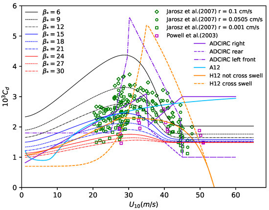
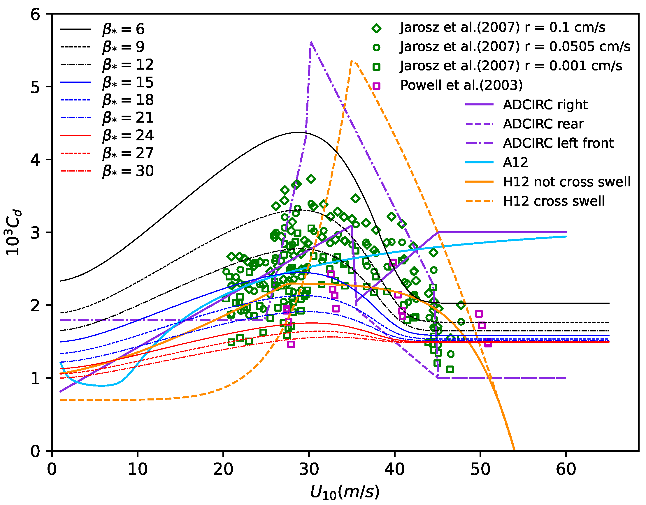
The comparison between the above-mentioned three parameterizations and our new parameterizations, along with two field observations, are presented in Figure 10 because the curves of our parameterization only show a little difference for different $H_s$ parameterization as shown in Figure 8 and Figure 9, we only plot the curves based on the $H_s$ parameterization of Wang et al. [82]. The results in Figure 10 show that the saturation of $C_d$ are presented in different forms, all three forms of ADCIRC take $C_d$ as constants for $U_{10}$ > 45 m/s, but the values are different, the maximum value of $C_d$ predicted by ADCIRC left front is about 0.0057, which is much larger than that observed in field experiments; another problem for ADCIRC parameterization is that their values of $C_d$ are not continuous at their demarcation point of their formula, such as $U_{10}$ = 30 m/s, $U_{10}$ = 35 m/s, and $U_{10}$ = 45 m/s, which are unreasonable physically. The curve of A12 is smooth, but the reduction of $C_d$ at $U_{10}$ > 35 m/s has not been reproduced by their formula. $C_d$ predicted by H12 under cross swell conditions reaches a maximum value of about 0.0053 at $U_{10}\approx 35$ m/s, then decreases rapidly, the predicted $C_d$ is smaller than 0 when $U_{10}$ > 54 m/s, this is also incorrect. In general, these three schemes have deficiencies in different aspects, our parameterization has presented the most reasonable results.

Figure 10. As in Figure 8c, but the curves of ADCIRC, A12, and H12 are plotted.

6. Conclusions

An accurate estimate of momentum transfer across the air–sea interface is vital for atmospheric, oceanic, and surface wave prediction models. Compared with parameterization of momentum flux based on wind speed, parameterization based on wave state can describe the nature of the air–sea interface more directly. Wave age ($\beta =c_p/U_{10}$, or ${\beta }_{*}=c_p/u_{*}$) and wave steepness ($\delta =H_s/L_p$) are two of the most frequently used parameters to describe the air–sea interface and the development of wind wave. Using eight observational datasets, the performances of two most widely used wave state related parameterizations: TY01 and DN03, are examined under various wave conditions. TY01 shows a better performance for the younger waves (smaller ${\beta }_{*}$), while DN03 is more suitable for wave fields with medium or large wave age. Hence, we use a combination of them to get a better performance under various wave conditions: for ${\beta }_{*}<15.21$, TY01 is adopted; and, for ${\beta }_{*}\ge 15.21$, DN03 is adopted. The demarcation point ${\beta }_{*}=15.21$ is selected from the $\delta -{\beta }_{*}$ relationship derived from Toba’s [72] 3/2 power law (see Equation (22)). Considering that TY01 and DN03 were developed using observational data under low and moderate wind speed conditions ($U_{10}\le 20$ m/s), the effect of sea foam was not included explicitly or implicitly in the proposing of TY01 and DN03. By introducing the effect of sea foam into the scheme presented in Section 3 (see Equation (23)), a new parameterization of sea surface roughness based on the wave state and sea foam is proposed (see Equation (29)).

$C_d$ predicted by the new parameterization increases with wind speed in the range of 0∼30 m/s; the maximum values are reached at about 30∼35 m/s and then decrease at the wind speed about 35∼45 m/s under the effect of sea foam; its behavior is also supported by the field observations from [29,68]. The saturation values of $C_d$ in laboratory measurements from [27,28] is also reproduced by the new parameterization.

Due to the vital role of wave state and sea foam on the momentum transfer across the air–sea interface, the new proposed sea surface roughness parameterization is suitable for the coupled atmosphere-ocean-wave modeling systems. Furthermore, as the effects of sea foam are included in the presented parameterization, it is also applicable for the modeling of some severe air–sea interaction activities accompanied with extreme winds, such as tropical cyclones, and the wave modeling of storm surge.

Finally, it should be emphasized that, due to the lack of simultaneous wave state measurements under high wind speed conditions, the values predicted by the new parameterization have not been compared with the observational data directly. Thus, more field and laboratory experiments containing simultaneous wind and wave state measurements, especially for high wind speed conditions, are needed to further verify the performance of the new parameterization, and to investigate the specific mechanism of air–sea interaction. However, although a direct comparison between the new parameterization with the observational data at high wind speeds is difficult, assessing it in the numerical weather prediction system is more realistic. It is our plan to implement the new parameterization in numerical models, including large-eddy simulations and coupled atmosphere-wave models, and to evaluate the performance of our parameterization from the model results.

References

- Kumar, R.; Sandeepan, B.; Holland, D.M. Impact of different sea surface roughness on surface gravity waves using a coupled atmosphere–wave model: A case of Hurricane Isaac (2012). Ocean Dyn. 2020, 70, 421–433. [Google Scholar] [CrossRef] [Scilit]
- Golbraikh, E.; Shtemler, Y.M. Momentum and heat transfer across the foam-covered air–sea interface in hurricanes. Ocean Dyn. 2020, 70, 683–692. [Google Scholar] [CrossRef] [Scilit]
- Yousefi, K.; Veron, F.; Buckley, M.P. Momentum flux measurements in the airflow over wind-generated surface waves. J. Fluid Mech. 2020, 895. [Google Scholar] [CrossRef] [Scilit]
- Bye, J.A.; Jenkins, A.D. Drag coefficient reduction at very high wind speeds. J. Geophys. Res. Ocean. 2006, 111. [Google Scholar] [CrossRef] [Scilit]
- Priestley, C.H.B. Turbulent Transfer in the Lower Atmosphere; CSIRO: Canberra, Australia, 1959. [Google Scholar]
- Lumley, J.; Panofsky, H. The structure of atmospheric turbulence. New York. Interscience Publ. MacPherson, J. y GA Isaac, 1977. Turbulent characteristics of some Canadian cumulus clouds. J. Appl. Meteorx. 1964, 16, 81–90. [Google Scholar]
- Webb, E.K. Profile relationships: The log-linear range, and extension to strong stability. Q. J. R. Meteorol. Soc. 1970, 96, 67–90. [Google Scholar] [CrossRef] [Scilit]
- Paulson, C.A. The mathematical representation of wind speed and temperature profiles in the unstable atmospheric surface layer. J. Appl. Meteorol. 1970, 9, 857–861. [Google Scholar] [CrossRef] [Scilit]
- Grachev, A.A.; Andreas, E.L.; Fairall, C.W.; Guest, P.S.; Persson, P.O.G. SHEBA flux–profile relationships in the stable atmospheric boundary layer. Bound.-Layer Meteorol. 2007, 124, 315–333. [Google Scholar] [CrossRef] [Scilit]
- Smith, S.D. Wind stress and heat flux over the ocean in gale force winds. J. Phys. Oceanogr. 1980, 10, 709–726. [Google Scholar] [CrossRef] [Scilit]
- Smith, S.D.; Anderson, R.J.; Oost, W.A.; Kraan, C.; Maat, N.; De Cosmo, J.; Katsaros, K.B.; Davidson, K.L.; Bumke, K.; Hasse, L.; et al. Sea surface wind stress and drag coefficients: The HEXOS results. Bound.-Layer Meteorol. 1992, 60, 109–142. [Google Scholar] [CrossRef] [Scilit]
- Geernaert, G.; Larsen, S.; Hansen, F. Measurements of the wind stress, heat flux, and turbulence intensity during storm conditions over the North Sea. J. Geophys. Res. Ocean. 1987, 92, 13127–13139. [Google Scholar] [CrossRef] [Scilit]
- Edson, J.B.; Jampana, V.; Weller, R.A.; Bigorre, S.P.; Plueddemann, A.J.; Fairall, C.W.; Miller, S.D.; Mahrt, L.; Vickers, D.; Hersbach, H. On the exchange of momentum over the open ocean. J. Phys. Oceanogr. 2013, 43, 1589–1610. [Google Scholar] [CrossRef] [Scilit]
- Guan, C.; Xie, L. On the linear parameterization of drag coefficient over sea surface. J. Phys. Oceanogr. 2004, 34, 2847–2851. [Google Scholar] [CrossRef] [Scilit]
- Kondo, J. Air-sea bulk transfer coefficients in diabatic conditions. Bound.-Layer Meteorol. 1975, 9, 91–112. [Google Scholar] [CrossRef] [Scilit]
- Smith, S.; Banke, E. Variation of the sea surface drag coefficient with wind speed. Q. J. R. Meteorol. Soc. 1975, 101, 665–673. [Google Scholar] [CrossRef]
- Garratt, J. Review of drag coefficients over oceans and continents. Mon. Weather Rev. 1977, 105, 915–929. [Google Scholar] [CrossRef] [Scilit]
- Wu, J. Wind-stress coefficients over sea surface near neutral conditions—A revisit. J. Phys. Oceanogr. 1980, 10, 727–740. [Google Scholar] [CrossRef] [Scilit]
- Large, W.; Pond, S. Open ocean momentum flux measurements in moderate to strong winds. J. Phys. Oceanogr. 1981, 11, 324–336. [Google Scholar] [CrossRef] [Scilit]
- Donelan, M.A. The dependence of the aerodynamic drag coefficient on wave parameters. In Proceedings of the First, International Conference on meteorological and Air–Sea Interaction of the Coastal Zone, The Hague, The Netherlands, 10–12 May 1982; American Meteorological Society: Boston, MA, USA, 1982; pp. 381–387. [Google Scholar]
- Yelland, M.; Taylor, P.K. Wind stress measurements from the open ocean. J. Phys. Oceanogr. 1996, 26, 541–558. [Google Scholar] [CrossRef] [Scilit]
- Vickers, D.; Mahrt, L. Fetch limited drag coefficients. Bound.-Layer Meteorol. 1997, 85, 53–79. [Google Scholar] [CrossRef] [Scilit]
- Drennan, W.M.; Graber, H.C.; Donelan, M.A. Evidence for the effects of swell and unsteady winds on marine wind stress. J. Phys. Oceanogr. 1999, 29, 1853–1864. [Google Scholar] [CrossRef] [Scilit]
- Toffoli, A.; Loffredo, L.; Le Roy, P.; Lefèvre, J.M.; Babanin, A. On the variability of sea drag in finite water depth. J. Geophys. Res. Ocean. 2012, 117. [Google Scholar] [CrossRef] [Scilit]
- Bender, M.A.; Ginis, I.; Kurihara, Y. Numerical simulations of tropical cyclone-ocean interaction with a high-resolution coupled model. J. Geophys. Res. Atmos. 1993, 98, 23245–23263. [Google Scholar] [CrossRef] [Scilit]
- Tolman, H.L.; Balasubramaniyan, B.; Burroughs, L.D.; Chalikov, D.V.; Chao, Y.Y.; Chen, H.S.; Gerald, V.M. Development and implementation of wind-generated ocean surface wave Modelsat NCEP. Weather Forecast. 2002, 17, 311–333. [Google Scholar] [CrossRef] [Scilit]
- Donelan, M.; Haus, B.K.; Reul, N.; Plant, W.; Stiassnie, M.; Graber, H.C.; Brown, O.; Saltzman, E. On the limiting aerodynamic roughness of the ocean in very strong winds. Geophys. Res. Lett. 2004, 31. [Google Scholar] [CrossRef] [Scilit]
- Takagaki, N.; Komori, S.; Suzuki, N.; Iwano, K.; Kuramoto, T.; Shimada, S.; Kurose, R.; Takahashi, K. Strong correlation between the drag coefficient and the shape of the wind sea spectrum over a broad range of wind speeds. Geophys. Res. Lett. 2012, 39. [Google Scholar] [CrossRef] [Scilit]
- Powell, M.D.; Vickery, P.J.; Reinhold, T.A. Reduced drag coefficient for high wind speeds in tropical cyclones. Nature 2003, 422, 279–283. [Google Scholar] [CrossRef] [Scilit]
- Zijlema, M.; Van Vledder, G.P.; Holthuijsen, L. Bottom friction and wind drag for wave models. Coast. Eng. 2012, 65, 19–26. [Google Scholar] [CrossRef] [Scilit]
- Green, B.W.; Zhang, F. Impacts of air–sea flux parameterizations on the intensity and structure of tropical cyclones. Mon. Weather Rev. 2013, 141, 2308–2324. [Google Scholar] [CrossRef] [Scilit]
- Chen, Y.; Zhang, F.; Green, B.W.; Yu, X. Impacts of ocean cooling and reduced wind drag on Hurricane Katrina (2005) based on numerical simulations. Mon. Weather Rev. 2018, 146, 287–306. [Google Scholar] [CrossRef] [Scilit]
- Moon, I.J.; Kwon, J.I.; Lee, J.C.; Shim, J.S.; Kang, S.K.; Oh, I.S.; Kwon, S.J. Effect of the surface wind stress parameterization on the storm surge modeling. Ocean Model. 2009, 29, 115–127. [Google Scholar] [CrossRef] [Scilit]
- Bryant, K.M.; Akbar, M. An exploration of wind stress calculation techniques in hurricane storm surge modeling. J. Mar. Sci. Eng. 2016, 4, 58. [Google Scholar] [CrossRef] [Scilit]
- Troitskaya, Y.I.; Sergeev, D.; Kandaurov, A.; Baidakov, G.; Vdovin, M.; Kazakov, V. Laboratory and theoretical modeling of air–sea momentum transfer under severe wind conditions. J. Geophys. Res. Ocean. 2012, 117. [Google Scholar] [CrossRef] [Scilit]
- Takagaki, N.; Komori, S.; Suzuki, N.; Iwano, K.; Kurose, R. Mechanism of drag coefficient saturation at strong wind speeds. Geophys. Res. Lett. 2016, 43, 9829–9835. [Google Scholar] [CrossRef] [Scilit]
- Komori, S.; Iwano, K.; Takagaki, N.; Onishi, R.; Kurose, R.; Takahashi, K.; Suzuki, N. Laboratory measurements of heat transfer and drag coefficients at extremely high wind speeds. J. Phys. Oceanogr. 2018, 48, 959–974. [Google Scholar] [CrossRef] [Scilit]
- Makin, V.K. A note on the drag of the sea surface at hurricane winds. Bound.-Layer Meteorol. 2005, 115, 169–176. [Google Scholar] [CrossRef] [Scilit]
- Troitskaya, Y.; Ezhova, E.; Soustova, I.; Zilitinkevich, S. On the effect of sea spray on the aerodynamic surface drag under severe winds. Ocean Dyn. 2016, 66, 659–669. [Google Scholar] [CrossRef] [Scilit]
- Rastigejev, Y.; Suslov, S.A. E–ε model of spray-laden near-sea atmospheric layer in high wind conditions. J. Phys. Oceanogr. 2014, 44, 742–763. [Google Scholar] [CrossRef] [Scilit]
- Kudryavtsev, V.N.; Makin, V.K. Aerodynamic roughness of the sea surface at high winds. Bound.-Layer Meteorol. 2007, 125, 289–303. [Google Scholar] [CrossRef] [Scilit]
- Kukulka, T.; Hara, T.; Belcher, S.E. A model of the air–sea momentum flux and breaking-wave distribution for strongly forced wind waves. J. Phys. Oceanogr. 2007, 37, 1811–1828. [Google Scholar] [CrossRef] [Scilit]
- Liu, B.; Guan, C.; Xie, L. The wave state and sea spray related parameterization of wind stress applicable from low to extreme winds. J. Geophys. Res. Ocean. 2012, 117. [Google Scholar] [CrossRef] [Scilit]
- Moon, I.J.; Ginis, I.; Hara, T. Effect of surface waves on air–sea momentum exchange. Part II: Behavior of drag coefficient under tropical cyclones. J. Atmos. Sci. 2004, 61, 2334–2348. [Google Scholar] [CrossRef] [Scilit]
- Toba, Y.; Iida, N.; Kawamura, H.; Ebuchi, N.; Jones, I.S. Wave dependence of sea-surface wind stress. J. Phys. Oceanogr. 1990, 20, 705–721. [Google Scholar] [CrossRef] [Scilit]
- Donelan, M.A.; Dobson, F.W.; Smith, S.D.; Anderson, R.J. On the dependence of sea surface roughness on wave development. J. Phys. Oceanogr. 1993, 23, 2143–2149. [Google Scholar] [CrossRef] [Scilit]
- Hwang, P.A. Temporal and spatial variation of the drag coefficient of a developing sea under steady wind-forcing. J. Geophys. Res. Ocean. 2005, 110. [Google Scholar] [CrossRef] [Scilit]
- Zhao, D.; Li, M. Dependence of wind stress across an air–sea interface on wave states. J. Oceanogr. 2019, 75, 207–223. [Google Scholar] [CrossRef] [Scilit]
- Drennan, W.M.; Graber, H.C.; Hauser, D.; Quentin, C. On the wave age dependence of wind stress over pure wind seas. J. Geophys. Res. Ocean. 2003, 108. [Google Scholar] [CrossRef] [Scilit]
- Anctil, F.; Donelan, M. Air–water momentum flux observations over shoaling waves. J. Phys. Oceanogr. 1996, 26, 1344–1353. [Google Scholar] [CrossRef] [Scilit]
- Taylor, P.K.; Yelland, M.J. The dependence of sea surface roughness on the height and steepness of the waves. J. Phys. Oceanogr. 2001, 31, 572–590. [Google Scholar] [CrossRef] [Scilit]
- Drennan, W.M.; Taylor, P.K.; Yelland, M.J. Parameterizing the sea surface roughness. J. Phys. Oceanogr. 2005, 35, 835–848. [Google Scholar] [CrossRef] [Scilit]
- Olabarrieta, M.; Warner, J.C.; Armstrong, B.; Zambon, J.B.; He, R. Ocean–atmosphere dynamics during Hurricane Ida and Nor’Ida: An application of the coupled ocean–atmosphere–wave–sediment transport (COAWST) modeling system. Ocean Model. 2012, 43, 112–137. [Google Scholar] [CrossRef] [Scilit]
- Soloviev, A.V.; Lukas, R.; Donelan, M.A.; Haus, B.K.; Ginis, I. The air–sea interface and surface stress under tropical cyclones. Sci. Rep. 2014, 4, 5306. [Google Scholar] [CrossRef] [Scilit] [PubMed]
- Golbraikh, E.; Shtemler, Y.M. Foam input into the drag coefficient in hurricane conditions. Dyn. Atmos. Ocean. 2016, 73, 1–9. [Google Scholar] [CrossRef] [Scilit]
- Anctil, F.; Donelan, M.A.; Drennan, W.M.; Graber, H.C. Eddy-correlation measurements of air–sea fluxes from a discus buoy. J. Atmos. Ocean. Technol. 1994, 11, 1144–1150. [Google Scholar] [CrossRef] [Scilit]
- Anderson, R. A study of wind stress and heat flux over the open ocean by the inertial-dissipation method. J. Phys. Oceanogr. 1993, 23, 2153–2161. [Google Scholar] [CrossRef] [Scilit]
- Young, I.R.; Banner, M.L.; Donelan, M.A.; McCormick, C.; Babanin, A.V.; Melville, W.K.; Veron, F. An integrated system for the study of wind-wave source terms in finite-depth water. J. Atmos. Ocean. Technol. 2005, 22, 814–831. [Google Scholar] [CrossRef] [Scilit]
- Babanin, A.V.; Makin, V.K. Effects of wind trend and gustiness on the sea drag: Lake George study. J. Geophys. Res. Ocean. 2008, 113. [Google Scholar] [CrossRef] [Scilit]
- Dobson, F.W.; Smith, S.D.; Anderson, R.J. Measuring the relationship between wind stress and sea state in the open ocean in the presence of swell. Atmosphere-Ocean 1994, 32, 237–256. [Google Scholar] [CrossRef] [Scilit]
- Drennan, W.M.; Donelan, M.; Terray, E.; Katsaros, K. Oceanic turbulence dissipation measurements in SWADE. J. Phys. Oceanogr. 1996, 26, 808–815. [Google Scholar] [CrossRef] [Scilit]
- Donelan, M. The air–sea momentum flux in mixed wind sea and swell conditions. J. Phys. Oceanogr. 1997, 27, 2087–2099. [Google Scholar] [CrossRef] [Scilit]
- Janssen, J. Does wind stress depend on sea-state or not?–A statistical error analysis of Hexmax data. Bound.-Layer Meteorol. 1997, 83, 479–503. [Google Scholar] [CrossRef] [Scilit]
- Johnson, H.; Højstrup, J.; Vested, H.; Larsen, S.E. On the dependence of sea surface roughness on wind waves. J. Phys. Oceanogr. 1998, 28, 1702–1716. [Google Scholar] [CrossRef] [Scilit]
- Romero, L.; Melville, W.K. Airborne observations of fetch-limited waves in the Gulf of Tehuantepec. J. Phys. Oceanogr. 2010, 40, 441–465. [Google Scholar] [CrossRef] [Scilit]
- Brown, E.N.; Friehe, C.; Lenschow, D. The use of pressure fluctuations on the nose of an aircraft for measuring air motion. J. Clim. Appl. Meteorol. 1983, 22, 171–180. [Google Scholar] [CrossRef] [Scilit]
- Carter, D. Prediction of wave height and period for a constant wind velocity using the JONSWAP results. Ocean Eng. 1982, 9, 17–33. [Google Scholar] [CrossRef] [Scilit]
- Jarosz, E.; Mitchell, D.A.; Wang, D.W.; Teague, W.J. Bottom-up determination of air–sea momentum exchange under a major tropical cyclone. Science 2007, 315, 1707–1709. [Google Scholar] [CrossRef] [Scilit]
- Krogstad, H.E.; Wolf, J.; Thompson, S.P.; Wyatt, L.R. Methods for intercomparison of wave measurements. Coast. Eng. 1999, 37, 235–257. [Google Scholar] [CrossRef] [Scilit]
- Donelan, M.A. Air-sea interaction. Sea 1990, 9, 239–292. [Google Scholar]
- Ardhuin, F.; Rogers, E.; Babanin, A.V.; Filipot, J.F.; Magne, R.; Roland, A.; Van Der Westhuysen, A.; Queffeulou, P.; Lefevre, J.M.; Aouf, L.; et al. Semiempirical dissipation source functions for ocean waves. Part I: Definition, calibration, and validation. J. Phys. Oceanogr. 2010, 40, 1917–1941. [Google Scholar] [CrossRef] [Scilit]
- Toba, Y. Local balance in the air–sea boundary processes. J. Oceanogr. 1972, 28, 109–120. [Google Scholar] [CrossRef] [Scilit]
- Ebuchi, N.; Toba, Y.; Kawamura, H. Statistical study on the local equilibrium between wind and wind waves by using data from ocean data buoy stations. J. Oceanogr. 1992, 48, 77–92. [Google Scholar] [CrossRef] [Scilit]
- Guan, C.; Sun, Q. Analyses of wind wave growth relations and their support to the 3/2 power law. J. Ocean Univ. Qingdao 2001, 31, 633–639. [Google Scholar]
- Wen, S.; Zhang, D.; Guo, P.F.; Chen, B. Parameters in wind-wave frequency spectra and their bearings on spectrum forms and growth. Acta Oceanol. Sin 1989, 8, 15–39. [Google Scholar]
- Goda, Y. Investigation of the statistical properties of sea waves with field and simulation data. Rept. Port Harb. Res. Inst. 1974, 13, 3–37. [Google Scholar]
- Donelan, M.; Drennan, W. Direct field measurements of the flux of carbon dioxide. Air-Water Gas Transf. 1995, 677, 683. [Google Scholar]
- Hauser, D.; Branger, H.; Bouffies-Cloché, S.; Despiau, S.; Drennan, W.; Dupuis, H.; Durand, P.; Durrieu de Madron, X.; Estournel, C.; Eymard, L.; et al. The FETCH experiment: An overview. J. Geophys. Res. Ocean. 2003, 108. [Google Scholar] [CrossRef] [Scilit]
- Donelan, M.A.; Madsen, N.; Kahma, K.K.; Tsanis, I.K.; Drennan, W.M. Apparatus for atmospheric surface layer measurements over waves. J. Atmos. Ocean. Technol. 1999, 16, 1172–1182. [Google Scholar] [CrossRef] [Scilit]
- Holthuijsen, L.H.; Powell, M.D.; Pietrzak, J.D. Wind and waves in extreme hurricanes. J. Geophys. Res. Ocean. 2012, 117. [Google Scholar] [CrossRef] [Scilit]
- Fairall, C.W.; Bradley, E.F.; Hare, J.; Grachev, A.A.; Edson, J.B. Bulk parameterization of air–sea fluxes: Updates and verification for the COARE algorithm. J. Clim. 2003, 16, 571–591. [Google Scholar] [CrossRef] [Scilit]
- Wang, C.; Fei, J.; Ding, J.; Hu, R.; Huang, X.; Cheng, X. Development of a new significant wave height and dominant wave period parameterization scheme. Ocean Eng. 2017, 135, 170–182. [Google Scholar] [CrossRef] [Scilit]
- Young, I. A review of the sea state generated by hurricanes. Mar. Struct. 2003, 16, 201–218. [Google Scholar] [CrossRef] [Scilit]
- Powell, M. Final report to the NOAA Joint Hurricane Testbed: Drag coefficient distribution and wind speed dependence in tropical cyclones. NOAA Hurric. Res. Div. 2007. Available online: https://www.nhc.noaa.gov/jht/05-07reports/final_Powell_JHT07.pdf (accessed on 11 February 2021).
- Luettich, R.; Westerink, J. ADCIRC: A (Parallel) Advanced Circulation Model for Oceanic, Coastal and Estuarine Waters. Users Manual. 2000. Available online: http://www.marine.unc.edu/C_CATS/adcirc/adcirc.htm (accessed on 11 February 2021).
Publisher’s Note: MDPI stays neutral with regard to jurisdictional claims in published maps and institutional affiliations. |
© 2021 by the authors. Licensee MDPI, Basel, Switzerland. This article is an open access article distributed under the terms and conditions of the Creative Commons Attribution (CC BY) license (http://creativecommons.org/licenses/by/4.0/).