Modified Shields Number Considering the Vertical Seepage on Underwater Three-Dimensional Slopes

Abstract

Scour has been a topic of significant concern among coastal geotechnical engineers in recent years. The Shields number serves as a crucial parameter for erosion calculations, reflecting the balance between sediment particle conditions and hydrodynamic forces, derived from the mechanics of sediment particle equilibrium. Seepage flow, a common phenomenon driven by pressure in soil, further influences the movement of sediment particles. Building upon the classical three-dimensional two-slope angle erosion model, this study incorporates the vertical seepage force. It comprehensively considers slope angles, sediment response angles, incident current angles, and vertical seepage intensities to adjust the Shields number for sediment particles on slopes. The calculation encompasses both transverse and longitudinal slope configurations. Based on the derived formula and parametric analysis, the study draws the following conclusions: 1. The modified Shields number (${\theta }_{cr}/{\theta }_{cr0}$) decreases non-linearly with the increase of slope angle; 2. ${\theta }_{cr}/{\theta }_{cr0}$ is central and has axial symmetry about 180° incident current angles for transverse and longitudinal slopes, respectively; 3. ${\theta }_{cr}/{\theta }_{cr0}$ increases non-linearly with the increase of soil angle of response; 4. ${\theta }_{cr}/{\theta }_{cr0}$ decreases linearly with the increase of seepage intensity; 5. There exists an approximately zero ${\theta }_{cr}/{\theta }_{cr0}$ area when the response angle approaches the slope angle, and the area increases non-linearly as the seepage intensity becomes greater.

1. Introduction

In offshore and river channels, the scour problem is very common. The propagation of flow will generate a driving force on the sand particles, which will cause sand sliding, scrolling, or even jumping with violent fluid dynamics. It is therefore crucial to derive the critical moving state under various flow dynamics for different types of sand particles. It is well known that the dimensionless parameter Shields number is adopted for sand moving judgment, which is the ratio of the shear stress of the flow on the bed surface particle to the underwater gravity of the bed particle. In addition, the Shields number is a useful metric for assessing a variety of particulate matter, including fine clay, pebbles, and coarse gravel. As a result, it is widely applied in fields such as river erosion, sediment transport, coastal engineering, and the identification of debris flow initiation. Shields [1] was the first one who conducted foundational work and established the Shields parameter, a dimensionless number to predict the initiation of sediment motion, based on critical shear stress and particle size. Despite bed-load sediment, Rouse [2] conducted experiments to understand the mechanics of suspended sediment, focusing on the vertical distribution of suspended particles in flowing water. Coleman [3] provides a comprehensive overview of various experimental studies on sediment transport, including analyses of sediment motion dynamics and the application of the Shields number. Many researchers have investigated and summarized the Shields parameters calculation on a flat bed surface with different methods. Dey and Papanicolaou [4] present a comprehensive review of the important laboratory experimental and theoretical investigations on sediment threshold under steady stream flow, and the critical Shields number for sediment initiation on different types of beds and under various flow conditions was collected. Hinton et al. [5] compared different methods for predicting bed-load transport rates, in which seven sediment transport equations for bed-load transport were compared. Nasrollahi et al. [6] developed a two-dimensional (2D) computational model using the discrete element method (DEM) to simulate the initial sediment motion of non-cohesive uniform and non-uniform particles on a horizontal bed; sensitivity analysis was performed and the initiation mechanisms in different regions were investigated and the influence of different forces on the initiating particle motion was derived.

In the real environment, underwater slopes exist everywhere accompanied by scour development and the existing terrain. Therefore, the sloping effect is also a critical factor in scour calculation. As we all know, the commonly used Shields number is based on the assumption that the sand particle is located on a flat bed surface, and the sand particle is fully exposed without any shielding effect. Therefore, when a slope exists, the force balance between flow driving forces, gravity force, and friction resistance force is changed. Many researchers have committed to Shields number calculations on slopes, including two-dimensional (2D) and three-dimensional (3D) cases. Sekine and Parker [7] discussed the transport of sediment in the presence of transverse slopes, providing insights into the effects of bed slope on sediment movement, and the results were used to determine a relation for the ratio of transverse to streamwise bed-load transport. Wang and Yuan [8] investigated sediment transport over coarse-sand rippled beds under oscillatory flows; the main conclusion focused on the Shields number and ripple geometry. They pointed out that wave-driven near-bed oscillatory flows can be acceleration-skewed due to the onshore leaning of shoaling waves in shallow coastal waters. Ma et al. [9] used a two-phase model based on smoothed particle hydrodynamics (SPH) to describe water and sediment interactions. It employed an improved Shields criterion that accounts for sediment thickness and the slope of the sediment interface to predict sediment transport and erosion. Tan and Yuan [10] used a novel experimental setup to simulate nonlinear oscillatory flows over a sloping bed, providing detailed insights into sediment transport mechanisms with oscillatory flow acting on slope beds. The results improve the predictive capabilities of sediment transport models by accounting for both nonlinearity in wave shapes and bed slope effects, which are crucial for realistic coastal engineering applications. Salimi-Tarazouj et al. [11] utilized an Eulerian two-phase model, SedFoam, to simulate sediment transport over migrating ripples, highlighting the significant effects of wave shape, skewness, and asymmetry on sediment dynamics. The results pointed out the importance of considering underwater ripple terrain for coastal engineering and sediment management practices. According to the results, the asymmetric flow will reduce the net offshore directed suspended load transport rate. Meanwhile, compared to the asymmetric flow, the net onshore directed transport rate driven by the combined flow is slightly reduced, due to the small net offshore directed suspended transport rate. Therefore, the ripples certainly affect the ratio of suspended load and bed load, but it is also related to hydrodynamic conditions.

In the design of marine structures such as pipes, piles, and gravity foundations, scour prediction is very crucial to the safety of the structure. Many former researchers have investigated scour prediction through numerical and experimental methods. Sui et al. [12] employ a detailed 3D experimental approach to study sediment transport and scour dynamics around the suspended pipeline. They conclude that the primary stage of scour is driven by strong three-dimensional flow, while the secondary stage is slower and more two-dimensional, enhancing prediction accuracy for pipeline safety. Dodaro et al. [13,14] conducted flume experiments on the spatio and temporal evolution of downstream scouring results in a rigid bed, including new scouring results under steady-state and unsteady-state flow conditions. Furthermore, a new mathematical scouring model, namely the improved Einstein sediment transport method, was proposed, and the calculation results showed good comparison with experimental results. Tang et al. [15] provided a comprehensive numerical model to evaluate the impact of different breakwater configurations on coastal dynamics. It concludes that breakwater layout significantly affects wave patterns, sediment transport processes, and the resultant beach morphology, offering critical insights for optimizing coastal protection strategies. Lyu et al. [16] explored the intricate dynamics of scour formation around submerged mono-piles under the combined action of waves and currents, which provides insights into the mechanisms of local scour and the identification of factors influencing scour depth and patterns around a submerged mono-pile. Albayrak et al. [17] offered significant contributions by combining field data with numerical modelling to enhance understanding of sediment dynamics, which provides insights into tunnel design and maintenance for better performance and longevity under varying hydraulic conditions. The above studies all involve scour calculation in the vicinity of offshore and marine structures. However, little research was dedicated to Shields number modification while considering the existing seepage for a real scour environment.

It is evident that the scour is more likely to occur with the existing seepage [18,19,20,21]; if seepage is violent enough, the sand particles could move without horizontal flow drag force, such as sand surges and flowing soil after earthquakes generated by intense upward seepage. There has been some research focusing on the relationship between seepage and scour in recent decades. Qi and Gao [22] conducted experiments and indicated that the presence of combined waves and currents significantly influences the development and characteristics of local scour around mono-piles. Patel et al. [23,24] simulated the influence of downward seepage (i.e., leakage accident at the bottom of the open channel) on the scour around the series spur dike in the open channel flow through the flume experiment. According to the research results, the downward seepage movement leads to greater local scour at the leading edge of the spur dike. To prevent and reduce the damage caused by seepage, Sui et al. [25] conducted experiments to assess the effect of shell–sand mixing technology on coastal protection; the results indicate that the amplitude of pore water pressure decreased by up to 46.5% after the application of shell–sand mixing, and therefore the seepage result was greatly reduced. Takegawa et al. [26] conducted hydraulic model experiments to clarify the influence of liquefaction on the scour behind coastal dikes due to tsunami overflow; the results indicate that the degree of liquefaction was controlled by upward seepage and liquefaction notably changes the scour depth, length, and area, whereas the maximum scour depth and scour area for high hydraulic gradient became smaller than that for low hydraulic gradient. The experimental results show that significant seepage creates a longer but shallower scour profile, resulting in a smaller scour area. For example, at the end of the experiment, the scour length for $i=1.0$ is 1.20 and 1.59 times longer in $q=0.5$ and $q=1.0$, respectively, whereas the maximum scour depth for $i=1.0$ is 0.75 and 0.77 times smaller in $q=0.5$ and $q=1.0$, respectively, compared to $i=0.0$. In the research of Guo et al. [18], the effect of seepage flow on the mobility of bed particles was considered in the sediment incipient motion around a free-spanning pipeline. The results showed that lower saturation and higher seabed permeability increase seepage forces, increasing the mobility of bed particles. For sandy seabeds with lower shear modulus, where residual forces accumulate over time, this will facilitate particles being dragged away. Li et al. [19] proposed a numerical scour model considering the effect of upward seepage. Results show that the small seepage within the seabed can cause significant changes to the hydrodynamic force on the bed surface and stability of bed particles, which can significantly further affect the sediment transport. In the research of Zhai et al. [20], a modified Shields number considering the two-dimensional seepage was derived; the results indicated that two-dimensional seepage promoted the sediment incipient motion near wave troughs and restrained it near wave crests. Furthermore, Zhai et al. [21] proposed a numerical model considering the three-dimensional seepage in the process of sediment incipient motion; through parametric study, the results indicate that larger wave height, current velocity and soil permeability and smaller water depth, shear modulus and saturation degree remarkably increase the three-dimensional modified coefficient around the pile and further promote the sediment incipient motion and scour. This research highlights the necessity of including three-dimensional seepage in sediment transport models for more accurate predictions in coastal engineering. Numerical calculations such as two-dimensional seepage around pipeline [19,27,28,29] and three-dimensional seepage around pile [21,30] have been widely conducted. It should be pointed out that the derived equations have been adopted in the mentioned numerical studies. However, the derivation process and the influence of each scouring parameter are not detailed. Therefore, a 3D Shields number modification derivation considering the complex flow, terrain, and vertical seepage conditions is indispensable and necessary.

This study systematically investigates the effects of vertical upward seepage on a 3D slope sand particle moving; the flow, slope, and seepage parameters are considered to modify the critical Shields number. Additionally, conjoint calculation is adopted to analyse the 3D sloping effect and seepage effect; the modified Shields number variation distribution for a case study is depicted. The remainder of the present work is structured as follows: Section 2 presents the derivation for governing equations; Section 3 presents the parametric calculation results, comprising the effects of slope angle in Section 3.1, the effects of incident current angle in Section 3.2, the effects of soil angle of response in Section 3.3 and the effects of vertical seepage intensity in Section 3.4; Section 4 presents the collaborative calculation for parameters with two slopes; Finally, conclusions are presented in Section 5.

2. Critical Shields Number Formula Derivation

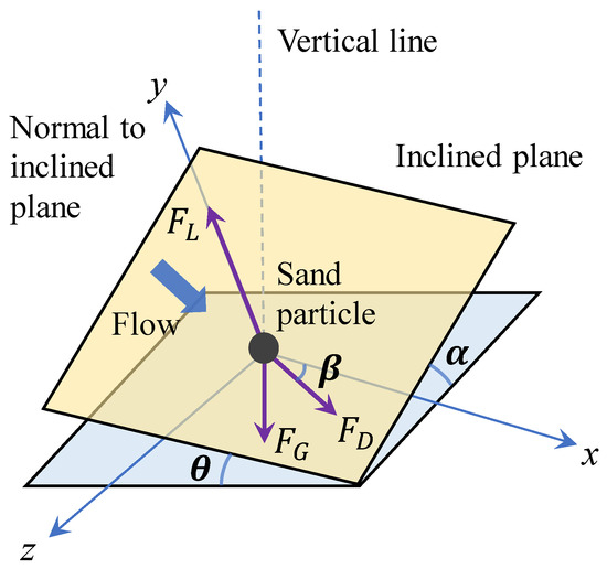
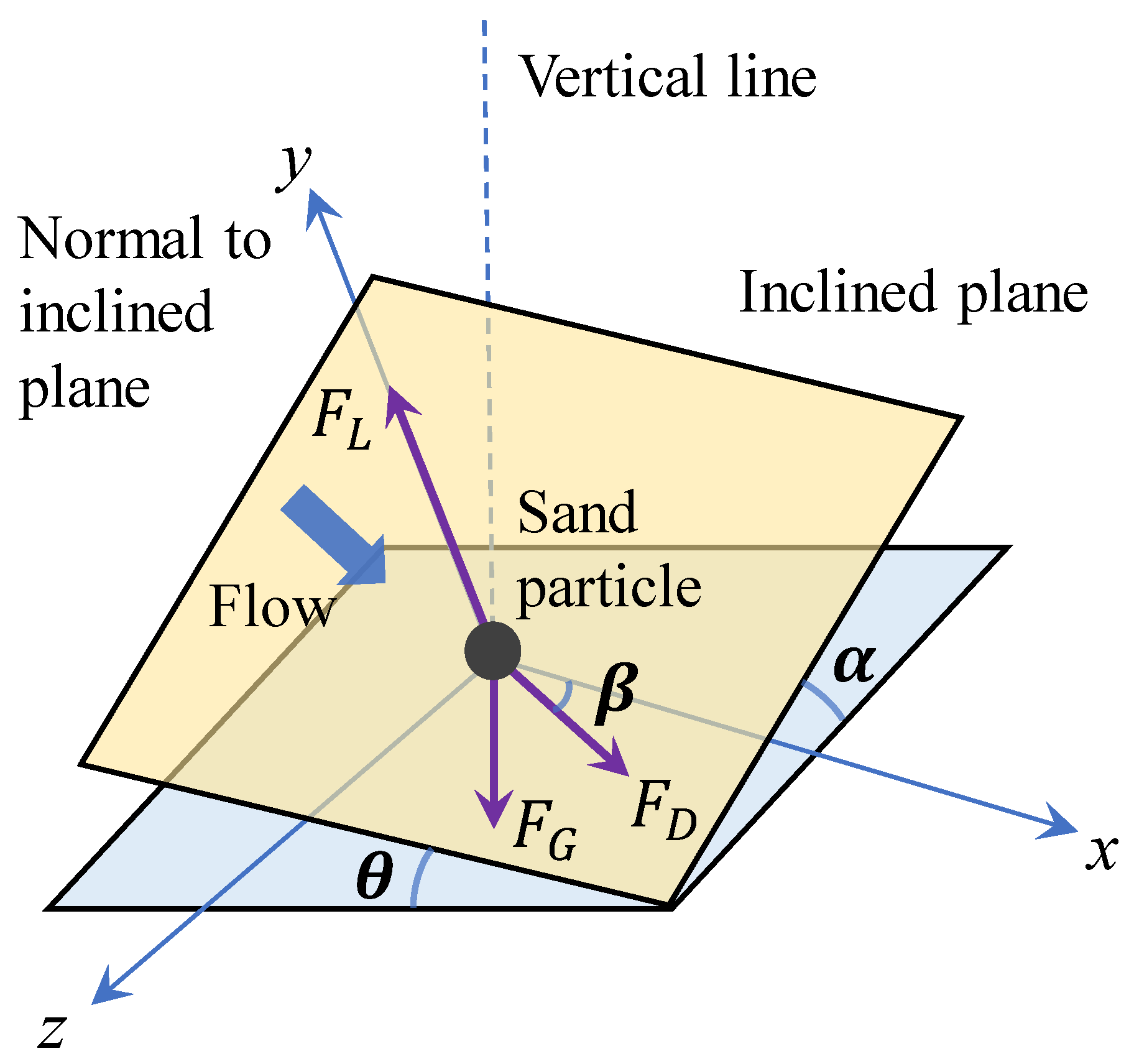
As shown in Figure 1, which is introduced in Dey [31], the force acting on a spherical sediment particle placed on a bed having a combined transverse and longitudinal slope is depicted. The forces include submerged weight of the particle ($F_G$), drag force ($F_D$), and lift force ($F_L$). However, when considering a vertical seepage force, e.g., tsunami-induced violent upward seepage loading, the vertical seepage force acting on the particle ($F_{vs}$) should be involved. The seepage force normal to the flat bed surface $F_{vs}$ is expressed as Cheng and Chiew [32],

$$\begin{array}{cc}\hfill & F_{vs}={\displaystyle \frac{i\rho g\pi d^3}{6(1-n)}}\hfill \\ \hfill & i_c=(S-1)(1-n)\hfill \end{array}$$

(1)

where n is the sand porosity. The seepage force acting on a porous medium per unit volume is expressed as $S=i\rho g$, (refer to Bear [33]). Furthermore, the number of sediment particles per unit volume is expressed as $N={\displaystyle \frac{1-n}{\pi d^3/6}}$, (refer to Cheng and Chiew [34]). The ratio of $S/N$ derives to the seepage force on a single particle in Equation (1). $i_c$ is the critical hydraulic gradient that describes the critical condition of liquefaction within the bed sediments. s is the specific gravity of sand particles, and n is the sand porosity.

Figure 1. Schematic photo of sand particle force balance on a 3D sloping seabed.

When the solitary particle maintains its position to avoid drop down, the drag force $F_D$, the seepage force $F_{vs}$ and the lift force $F_L$ could be decomposed into components on the slope surface; the force balance could be written as,

$$F_s^2={(F_{D}cos\beta +(F_G-F_{vs})sin\theta )}^2+{(F_{D}sin\beta +(F_G-F_{vs})cos\alpha )}^2$$

(2)

where $F_s$ is the static Coulomb friction force between the particle and the bed, and $\beta$ is the angle of inclination of flow with respect to the longitudinal axis of the channel (positive downward). The submerged weight of the particle is,

$$F_G={\displaystyle \frac{\pi }{6}}{d}^3({\rho }_s-\rho )g$$

(3)

where d is the particle diameter; ${\rho }_s$ is the mass density of particle; $\rho$ is the mass density of fluid; and g is the gravitational constant.

Combining Equations (1) and (3), one can get the seepage force $F_{vs}$ equals the sand gravity $F_G$ when $i=i_c$, and the relation between them is,

$$F_{vs}=F_G\ast {\displaystyle \frac{i}{i_c}}$$

(4)

The drag force and the lift force acting on the particle are,

$$\begin{array}{cc}\hfill F_D& =C_D{\displaystyle \frac{\pi d^2}{8}}\rho u_r^2;\hfill \\ \hfill F_L& =C_L{\displaystyle \frac{\pi d^2}{8}}\rho u_r^2\hfill \end{array}$$

(5)

where $C_D$ and $C_L$ are the drag and lift coefficients, the relative velocity $u_r$ relates to the fluid velocity u at the particle position, and the mean transport velocity of the particle moving as bed-load is $u_b$. It should be noted that the research focuses on the initiation calculation of a fully exposed sediment particle—complex conditions of multi-layer sediment and sheltered state are not involved. As pointed out by Engelund and Fredsøe [35], the value of u is denoted as $u=a{u}_f$, and $u_f$ is the friction velocity; a is an empirical constant taken as 10 with the experimental data from studies of Fernandez Luque and Van Beek [36] and Meland and Norrman [37] (note that a in the research of Engelund and Fredsøe [35] was determined by comparing the velocity of bed-load particles expressed by ${\displaystyle \frac{u_b}{u_f}}=a(1-0.7\sqrt{{\displaystyle \frac{{\theta }_c}{\theta }}})$). $\theta$ and ${\theta }_c$ are the Shields parameter and the critical Shields value, respectively.

The static Coulomb friction force $F_s$ is equal to,

$$F_s=((F_G-F_{vs})\sqrt{{cos}^2\theta -{sin}^2\alpha }-F_L){\mu }_c$$

(6)

where ${\mu }_c$ is the static Coulomb friction factor, and arctan(${\mu }_c$) equals the response angle $\mathsf{\Phi }$ for the submerged particles.

Equating Equations (2), (4) and (6), the force balance equation transforms to,

$$\begin{array}{cc}\hfill F_D^2+& 2F_D{F}_G(1-{\displaystyle \frac{i}{i_c}})(cos\beta sin\theta +sin\beta sin\alpha )+F_G^2{(1-{\displaystyle \frac{i}{i_c}})}^2({sin}^2\theta +{sin}^2\alpha )\hfill \\ \hfill -& {\left[F_G(1-{\displaystyle \frac{i}{i_c}})\sqrt{{cos}^2\theta -{sin}^2\alpha }-F_L\right]}^2{tan}^2\mathsf{\Phi }=0\hfill \end{array}$$

(7)

Normalizing Equation (7), we obtain,

$$\begin{array}{cc}\hfill & \left(1-{\eta }^2{tan}^2\varphi \right){\widehat{\tau }}_b^2\hfill \\ \hfill & +{\displaystyle \frac{2}{{\widehat{F}}_D}}\left(cos\beta sin\theta (1-{\displaystyle \frac{i}{i_c}})+sin\beta sin\alpha (1-{\displaystyle \frac{i}{i_c}})+\eta {tan}^2\varphi ·(1-{\displaystyle \frac{i}{i_c}})·\sqrt{{cos}^2\theta -{sin}^2\alpha }\right)·{\widehat{\tau }}_b\hfill \\ \hfill & -{\displaystyle \frac{1}{{\widehat{F}}_D}}\left[\left({cos}^2\theta -{sin}^2\alpha \right)·{(1-{\displaystyle \frac{i}{i_c}})}^2·{tan}^2\varphi -{sin}^2\theta {(1-{\displaystyle \frac{i}{i_c}})}^2-{sin}^2\alpha {(1-{\displaystyle \frac{i}{i_c}})}^2\right]=0\hfill \end{array}$$

(8)

where $\eta$ is $F_L/F_D$; ${\widehat{\tau }}_b$ is the dimensionless critical shear stress on a sloping bed, which is $\rho u_{\ast b}^2/\left[({\rho }_s-\rho )gd\right]$ or ${\tau }_b/\left[({\rho }_s-\rho )gd\right]$; $u_{\ast b}$ is the critical shear velocity on a sloping bed; ${\tau }_b$ is the critical shear stress on a sloping bed; and $\widehat{F_D}$ is equal to $6F_D/\left(\pi \rho d^2{u}_{\ast b}^2\right)$.

The positive solution of Equation (8) is,

$$\begin{array}{cc}\hfill {\widehat{\tau }}_b=& {\displaystyle \frac{1}{\left(1-{\eta }^2{tan}^2\varphi \right){\widehat{F}}_D}}\left\{-(cos\beta sin\theta (1-{\displaystyle \frac{i}{i_c}})+sin\beta sin\alpha (1-{\displaystyle \frac{i}{i_c}})\right.\hfill \\ \hfill & +\eta {tan}^2\varphi (1-{\displaystyle \frac{i}{i_c}})\sqrt{{cos}^2\theta -{sin}^2\alpha })+\left[(cos\beta sin\theta (1-{\displaystyle \frac{i}{i_c}})\right.\hfill \\ \hfill & +sin\beta sin\alpha (1-{\displaystyle \frac{i}{i_c}})+\eta {tan}^2\varphi (1-{\displaystyle \frac{i}{i_c}})\sqrt{{cos}^2\theta -{sin}^2\alpha })\hfill \\ \hfill & +(1-{\eta }^2{tan}^2\varphi )\left({cos}^2\theta {tan}^2\varphi {(1-{\displaystyle \frac{i}{i_c}})}^2-{sin}^2\alpha {tan}^2\varphi {(1-{\displaystyle \frac{i}{i_c}})}^2\right.\hfill \\ \hfill & \left.{\left.\left.-{sin}^2\theta {(1-{\displaystyle \frac{i}{i_c}})}^2-{sin}^2\alpha {(1-{\displaystyle \frac{i}{i_c}})}^2\right)\right]}^{0.5}\right\}\hfill \end{array}$$

(9)

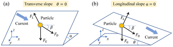
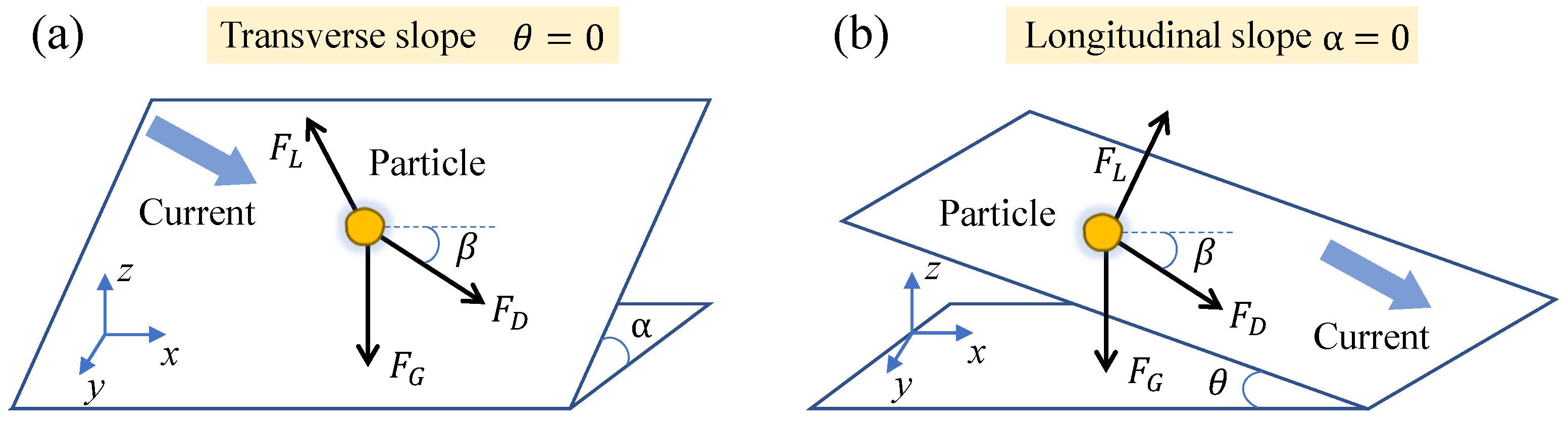
It is noted that in the schematic diagram in Figure 1, two slope directions are included, which are the transverse slope ($\theta =0$) and longitudinal slope ($\alpha =0$). As shown in Figure 2, the angle between flow direction and the positive x direction is defined as $\beta$. On the one hand, when the slope of $\theta$ is reduced to zero, as Figure 2a depicts, this is the transverse slope. On the other hand, when the slope of $\alpha$ is reduced to zero, as Figure 2b depicts, this is the longitudinal slope. In general, the former case is more common in constant direction flow channel circumstance, such as river scour. And the latter type of flow oblique to the bed slope is more usual in coastal and estuarine morphology. Thus, in this research, the transverse slope is firstly considered. For transverse slope, $\theta =0$, Equation (9) is written as follows,

$$\begin{array}{cc}\hfill {\widehat{\tau }}_b=& {\displaystyle \frac{1}{\left(1-{\eta }^2{tan}^2\varphi \right){\widehat{F}}_D}}\left\{-(sin\beta sin\alpha (1-{\displaystyle \frac{i}{i_c}})+(1-{\displaystyle \frac{i}{i_c}})·\eta ·{tan}^2\varphi \left.·cos\alpha \right)\right.\hfill \\ \hfill & +\left[\left(sin\beta sin\alpha (1-{\displaystyle \frac{i}{i_c}})+(1-{\displaystyle \frac{i}{i_c}})·\eta ·{tan}^2\varphi {\left.·cos\alpha \right)}^2+\left(1-{\eta }^2{tan}^2\varphi \right)\right.\right.\hfill \\ \hfill & ({tan}^2\varphi ·{(1-{\displaystyle \frac{i}{i_c}})}^2-{sin}^2\alpha ·{tan}^2\varphi ·{(1-{\displaystyle \frac{i}{i_c}})}^2\left.{\left.\left.-{sin}^2\alpha ·{(1-{\displaystyle \frac{i}{i_c}})}^2\right)\right]}^{0.5}\right\}\hfill \end{array}$$

(10)

Figure 2. Diagrammatic sketch of two kinds of slopes for a 3D sloping seabed. (a) Transverse slope; (b) longitudinal slope.

While for flat bed $\alpha =0$, and when the seepage force is not considered, ${\displaystyle \frac{i}{i_c}}=0$,

$$\begin{array}{cc}\hfill {\widehat{\tau }}_{b0}=& {\displaystyle \frac{1}{\left(1-{\eta }^2{tan}^2\varphi \right){\widehat{F}}_D}}\{-(1-{\displaystyle \frac{i}{i_c}})·\eta ·{tan}^2\varphi +[{(1-{\displaystyle \frac{i}{i_c}})}^2·{\eta }^2·{tan}^4\varphi \hfill \\ \hfill & +\left(1-{\eta }^2{tan}^2\varphi \right)·{tan}^2\varphi ·{(1-{\displaystyle \frac{i}{i_c}})}^2{]}^{0.5}\}\hfill \\ \hfill =& {\displaystyle \frac{(1-\eta tan\varphi )·tan\varphi }{(1-{\eta }^2{tan}^2\varphi )·{\widehat{F}}_D}}\hfill \end{array}$$

(11)

Thus, combining Equations (10) and (11), one can get,

$$\begin{array}{cc}\hfill {\displaystyle \frac{{\widehat{\tau }}_b}{{\widehat{\tau }}_{b0}}}=& {\displaystyle \frac{1}{\left(1-{\eta }^2{tan}^2\varphi \right){\widehat{F}}_D}}·\left\{\dots \dots \right\}·{\displaystyle \frac{(1-{\eta }^2{tan}^2\varphi )·{\widehat{F}}_D}{(1-\eta tan\varphi )·tan\varphi }}\hfill \\ \hfill =& {\displaystyle \frac{1}{\left(1-\eta tan\varphi \right)·tan\varphi }}·\left\{\dots \dots \right\}\hfill \end{array}$$

(12)

where $\eta ={\displaystyle \frac{F_L}{F_D}}$ in most regular loading conditions, such as the scour results around offshore wind turbine pile foundations. And the working condition belongs to a large water depth with steady near-bed flow, where the lifting force is much smaller than the drag force when the gravity force is dominant [6] (while the drag force is dominant, the ratio is usually less than o(0.1)). Therefore, the lift force could be omitted, and the value of $\eta$ degenerates to zero. $\eta \approx 0$, and Equation (12) gives us,

$$\begin{array}{cc}\hfill {\displaystyle \frac{{\widehat{\tau }}_b}{{\widehat{\tau }}_{b0}}}=& {\displaystyle \frac{1}{{\mu }_s}}·\left\{-sin\alpha sin\beta ·(1-{\displaystyle \frac{i}{i_c}})+\sqrt{\left[-{sin}^2\alpha {cos}^2\beta ·{(1-{\displaystyle \frac{i}{i_c}})}^2+{\mu }_s^2·{(1-{\displaystyle \frac{i}{i_c}})}^2·{cos}^2\alpha \right]}\right\}\hfill \\ \hfill =& -{\displaystyle \frac{sin\alpha sin\beta ·(1-\frac{i}{i_c})}{{\mu }_s}}+\sqrt{{\displaystyle \frac{-{sin}^2\alpha {cos}^2\beta ·{(1-\frac{i}{i_c})}^2+{\mu }_s^2·{(1-\frac{i}{i_c})}^2·{cos}^2\alpha }{{\mu }_s^2}}}\hfill \\ \hfill =& cos\alpha ·(1-{\displaystyle \frac{i}{i_c}})\left(\sqrt{1-{\displaystyle \frac{{tan}^2\alpha {cos}^2\beta }{{\mu }_s^2}}}-{\displaystyle \frac{tan\alpha sin\beta }{{\mu }_s}}\right)\hfill \end{array}$$

(13)

Equation (13) is exactly the modified Shields number ratio when considering the transverse slope, the incident flow angle and the seepage force. In the most common equation from Roulund et al. [38] and Figure 2a, Equation (13) should make some symbols change because of different definitions. In Roulund et al. [38], the $\beta$ is slope angle, and $\alpha$ is the angle between flow direction and the down-slope direction. Therefore, by transforming $\alpha =\beta$ and $\beta ={90}^{\circ }-\alpha$, we can get the express of Equation (13) under the definition of Roulund et al. [38], and the influence of vertical seepage force is added, and when the seepage force is zero (${\displaystyle \frac{i}{i_c}}$ = 0), Equation (13) is exactly the same as Roulund et al. [38].

The longitudinal slope is manifested as $\alpha$ = 0. We combine Equation (9) and the flat bed with no seepage circumstance, Equation (11). The modified Shields number ratio considering longitudinal slope is written as,

$${\displaystyle \frac{{\theta }_{cr}}{{\theta }_{cr0}}}=cos\theta ·\left(1-{\displaystyle \frac{i}{i_c}}\right)\left(\sqrt{1-{\displaystyle \frac{{sin}^2\beta {tan}^2\theta }{{\mu }_s^2}}}-{\displaystyle \frac{tan\theta cos\beta }{{\mu }_s}}\right)$$

(14)

Adopting Equations (13) and (14) to make a parameter analysis, the influence of vertical seepage intensity, slope angle, incident current angle, and soil angle of response on the reduced Shields ratio is investigated in the following subsections. The input parameters are listed in Table 1. The slope angle $\alpha$ or $\theta$ ranges from $0^{\circ }$ to ${30}^{\circ }$ with an interval of 5, the incident wave angle $\beta$ ranges from $0^{\circ }$ to ${360}^{\circ }$ with an interval of 10, the vertical seepage intensity $i/i_c$ varies from 0 to 0.9 in increments of 0.1, and the soil angle of response $\varphi$ varies from ${20}^{\circ }$ to ${40}^{\circ }$ in increments of $2^{\circ }$. Meanwhile, the adopted standard parameters are marked with bold font. Therefore, without explanation, the former four parameters are ${15}^{\circ }$, ${90}^{\circ }$, 0.5 and ${32}^{\circ }$ as standard condition.

Table 1. Parametric analysis of reduced Shields ratio.

Parameters	Notation	Values	Units
Slope angle	$\alpha$	0, 5, 10, 15, 20, 25, 30	$\circ$
Incident current angle	$\beta$	0, 10, 20, 30, 40, 50, 60, 70, 80, 90, 100, 110, 120, 130, 140, 150, 160, 170, 180, 190, 200, 210, 220, 230, 240, 250, 260, 270, 280, 290, 300, 310, 320, 330, 340, 350, 360	$\circ$
Vertical seepage intensity	$i/i_c$	0, 0.1, 0.2, 0.3, 0.4, 0.5, 0.6, 0.7, 0.8, 0.9	-
Soil angle of response	$\varphi$	20, 22, 24, 26, 28, 30, 32, 34, 36, 38, 40	$\circ$

Note: Bold values indicate the standard parameters used in this study.

3. Parametric Analysis for Transverse and Longitudinal Slope Conditions

This section concentrates on different slope conditions with relation to the underwater scour Shields number; different influencing factors such as slope angle, incident current angle, soil angle of response and vertical seepage intensity are compared carefully.

3.1. Influence of Slope Angle

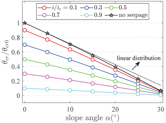
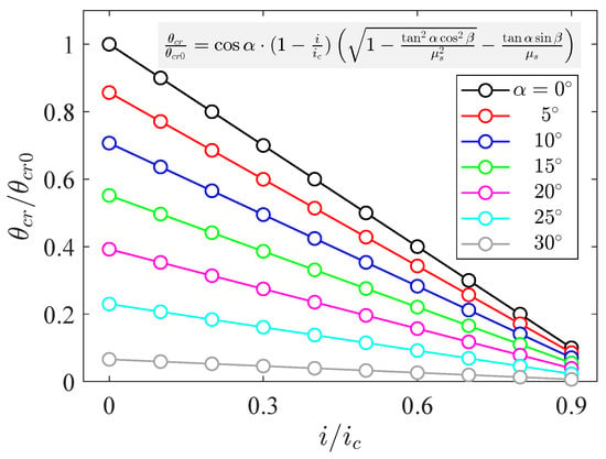
For the transverse slopes, as shown in Figure 3, the reduced Shields ratio decreases non-linearly with the increase of slope angle, regardless of whether the seepage force is considered or not. A black dashed line with linear variation is added to confirm the nonlinear variation. With a larger slope angle $\alpha$, the decreasing rate becomes much more significant. It is noted that when the seepage is not included, the reduced Shields ratio maintains the maximum in different slope cases. And when the slope $\alpha$ is zero, the circumstance transforms to the flat bed case without seepage, and the reduced Shields ratio is exactly one. In addition, with the increase of seepage intensity, the reduced Shields ratio regularly decreases. Another noteworthy conclusion is that when the seepage intensity becomes larger, the decrease rate of ${\theta }_{cr}/{\theta }_{cr0}$ gets more and more gentle; the intuitive manifestation is that the absolute gradient of the line from top to bottom ($i/i_c$ increases) becomes smaller. For example, when slope angle varies from $0^{\circ }$ to ${30}^{\circ }$, the results of $i/i_c$ = 0.1 vary from 0.9 to 0.059, and the results of $i/i_c$ = 0.9 vary from 0.1 to 0.006, which means the influence of slope angle on the reduced Shields ratio decreases under large seepage intensity. The reduced Shields ratio decreases non-linearly with larger slope angle, especially under $\alpha >{15}^{\circ }$. Because under larger seepage intensity and slope angle the critical Shields number is reduced, the sand particle can easily move and fall due to gravity and seepage force. Through the calculation of Equation (13), the effect is much more significant within that range.

Figure 3. Modified Shields number on a transverse slope with different slope angle $\alpha$.

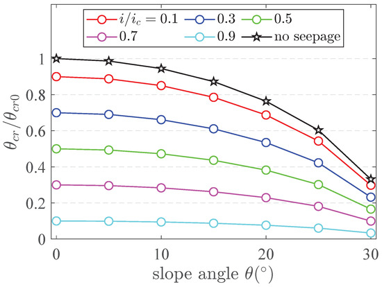
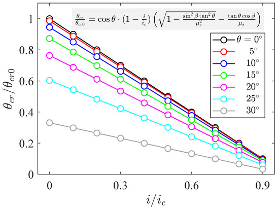
For the longitudinal slopes, as shown in Figure 4, the nonlinear relation between slope and ${\theta }_{cr}/{\theta }_{cr0}$ becomes more significant within the slope ranges from $0^{\circ }$ to ${30}^{\circ }$. Similarly, the decreasing rate of ${\theta }_{cr}/{\theta }_{cr0}$ becomes much more significant with a larger slope ratio. Even when the slope angle is ${30}^{\circ }$, there are still large differences between the results of ${\theta }_{cr}/{\theta }_{cr0}$ with different seepage intensities (${\displaystyle \frac{i}{i_c}}$), and ${\theta }_{cr}/{\theta }_{cr0}$ decreases 89% when ${\displaystyle \frac{i}{i_c}}$ increases from 0.1 to 0.9. The results indicate that ${\theta }_{cr}/{\theta }_{cr0}$ is more sensitive to the variation of slope angle for the transverse slopes; the larger variation range of ${\theta }_{cr}/{\theta }_{cr0}$ in transverse slopes is 5 times of the result in longitudinal slope. The control effect of slope geometry on the critical conditions for sediment initiation has significant spatial differences.

Figure 4. Modified Shields number on a longitudinal slope with different slope angle $\theta$.

3.2. Influence of Incident Current Angle

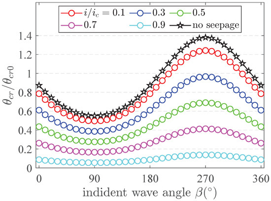
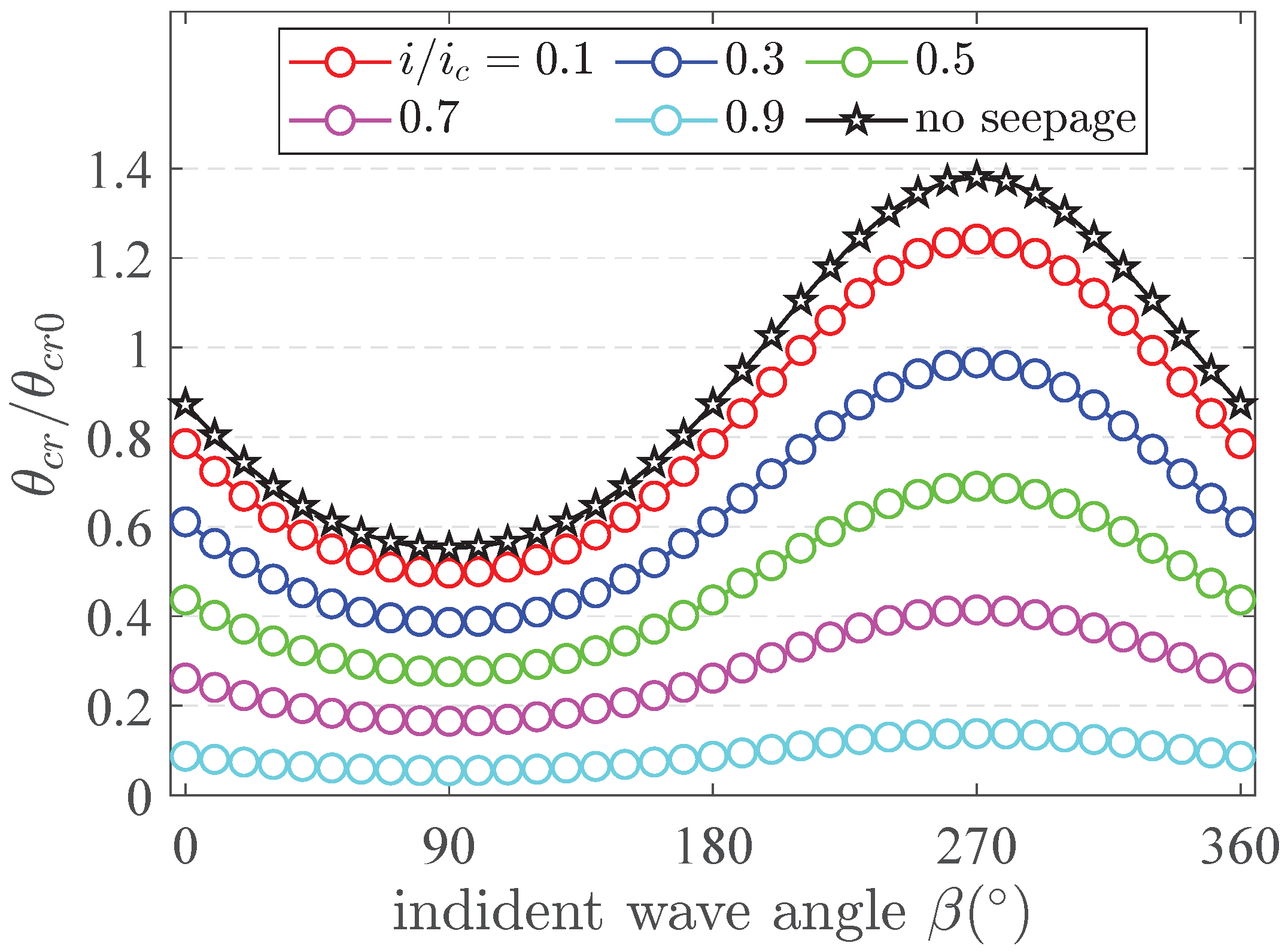
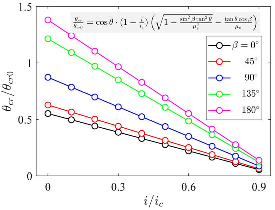
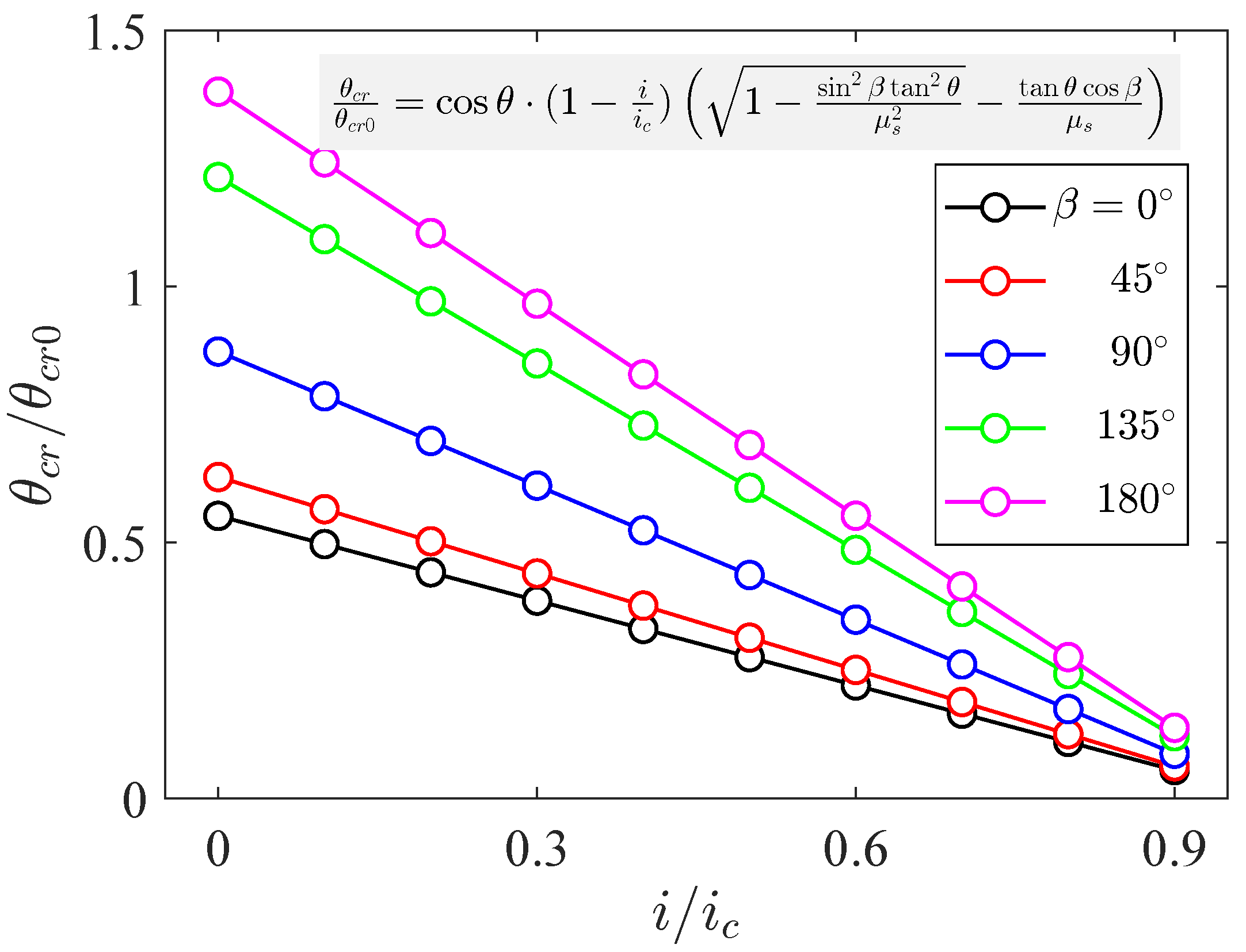
For the transverse slopes, as shown in Figure 5, in the range of $0^{\circ }$ to ${180}^{\circ }$, the reduced Shields ratio firstly decreases and then increases with the increase of incident current angle, regardless of whether the seepage force is considered or not. And the variation results are a central symmetry distribution about a ${180}^{\circ }$ position. When the incident wave angle $\alpha$ equals ${90}^{\circ }$, which means the incident current transport is along the down-slope direction (refer to Figure 2a), the reduced Shields ratio becomes the minimum due to the minimum friction resistance. When the incident current angle $\alpha$ equals ${270}^{\circ }$, which means the incident current transport is along the up-slope direction (refer to Figure 2a), the reduced Shields ratio becomes the maximum due to the maximum friction resistance resulting from the gravity component. In addition, with the increase of seepage intensity, the reduced Shields ratio regularly decreases. Another worthwhile thing to note from this result is that when the seepage intensity becomes larger, the variation rate of ${\theta }_{cr}/{\theta }_{cr0}$ gets more and more gentle; the intuitive behaviour is that the absolute tangent values of the line from top to bottom ($i/i_c$ increases) become smaller. For example, when the incident angle varies from $0^{\circ }$ to ${90}^{\circ }$, the results of $i/i_c$ = 0.1 vary from 0.496 to 1.242, and the results of $i/i_c$ = 0.9 vary from 0.055 to 0.138. A high seepage intensity ($i/i_c⩾0.7$) considerably reduces incident angle sensitivity.

Figure 5. Modified Shields number on a transverse slope with different incident current angle $\beta$.

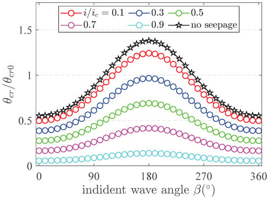
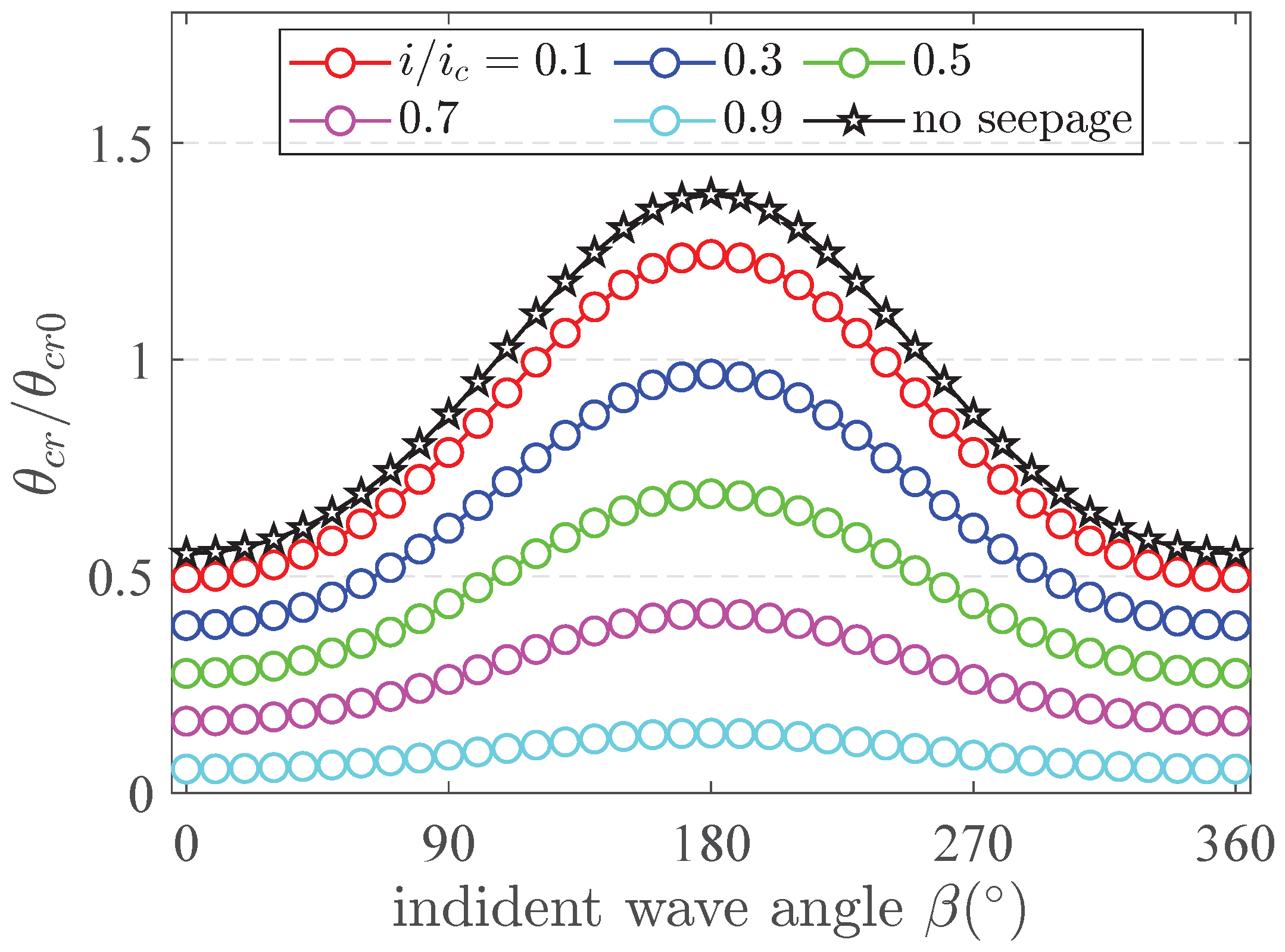
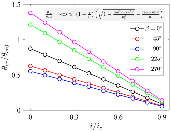
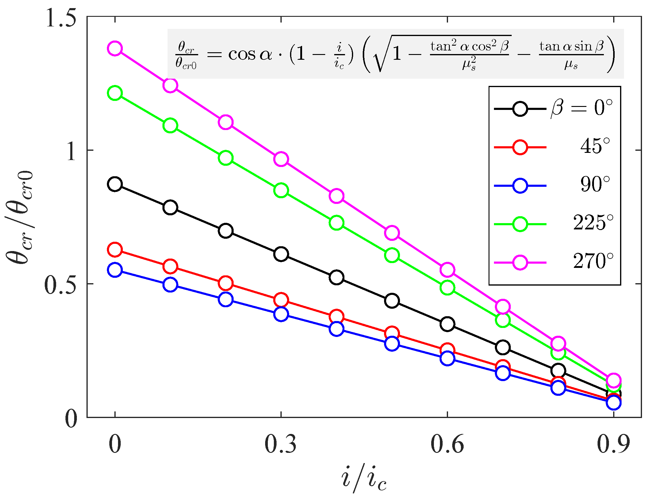
For the longitudinal slopes, as shown in Figure 6, with the increase of incident current angle $\beta$, ${\theta }_{cr}/{\theta }_{cr0}$ firstly increases from $0^{\circ }$ to ${180}^{\circ }$ and then decreases from ${180}^{\circ }$ to ${360}^{\circ }$, and the curves are axially symmetric about the ${180}^{\circ }$ position. When the incident current angle $\theta$ equals $0^{\circ }$ or ${360}^{\circ }$, which means the incident current transport is along the down-slope direction (refer to Figure 2b), similarly to what was mentioned above, ${\theta }_{cr}/{\theta }_{cr0}$ becomes the minimum due to the minimum friction resistance. And the ${180}^{\circ }$ incident current corresponds to the incident current transport being along the up-slope direction (refer to Figure 2b), where ${\theta }_{cr}/{\theta }_{cr0}$ becomes the maximum. The variation rate of the modified Shields number caused by the seepage intensity under the latter condition ($\beta ={180}^{\circ }$) is 2.3 times that of the former ($\beta =0^{\circ }$), indicating that down-slope flow has a stronger seepage effect. With the increase of seepage intensity, the value and its variation range of ${\theta }_{cr}/{\theta }_{cr0}$ become smaller.

Figure 6. Modified Shields number on a longitudinal slope with different incident current angle $\beta$.

3.3. Influence of Soil Angle of Response

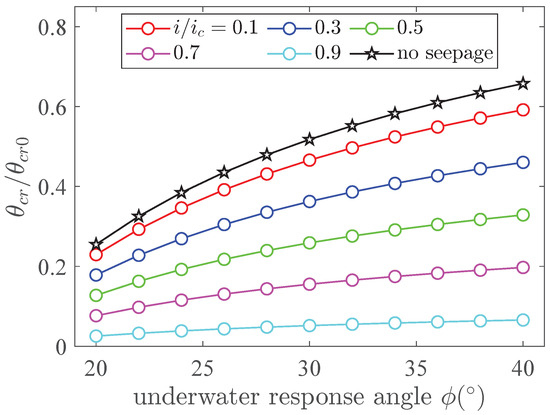
For the transverse slopes, as shown in Figure 7, the reduced Shields ratio increases with the increase of the underwater response angle $\varphi$ of soil, regardless of whether the seepage force is considered or not. It is noted that when the seepage is not included, the reduced Shields ratio maintains the maximum in all different slope cases. And with a larger response angle $\varphi$, ${\theta }_{cr}/{\theta }_{cr0}$ becomes larger, which is caused by the larger friction coefficient calculated by $tan\varphi$. Moreover, with the increase of seepage intensity, the reduced Shields ratio regularly decreases. Another phenomenon worth noting is that when the seepage intensity becomes larger, the variation rate of ${\theta }_{cr}/{\theta }_{cr0}$ gets more and more gentle; the intuitive view is that the gradient of the line from top to bottom ($i/i_c$ increases) becomes smaller. For example, when response angle varies from ${20}^{\circ }$ to ${40}^{\circ }$, the results of $i/i_c=0.1$ vary from 0.293 to 0.592, and the results of $i/i_c=0.9$ vary from 0.032 to 0.066. The results indicate that the impact of soil angle of response on critical starting parameters is considerably reduced under strong seepage conditions.

Figure 7. Modified Shields number on a transverse slope with different soil angle of response $\varphi$.

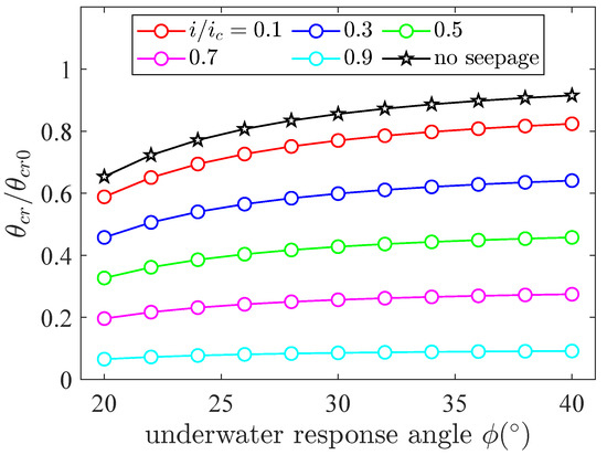
For the longitudinal slopes, as shown in Figure 8, the variation trend of ${\theta }_{cr}/{\theta }_{cr0}$ with response angle $\varphi$ is similar to the transverse slopes. However, the variation range of ${\theta }_{cr}/{\theta }_{cr0}$ is much smaller for different seepage intensity cases; even under large seepage intensity (such as 0.9), the variation curve behaves like a horizontal line with little change. In the typical underwater response angle range of sediment (${20}^{\circ }$ to ${40}^{\circ }$), the variation of ${\theta }_{cr}/{\theta }_{cr0}$ of the transverse slope is 2–3 times that of the longitudinal slope. The result indicates that ${\theta }_{cr}/{\theta }_{cr0}$ is more sensitive to the variation of soil angle of response for the transverse slopes. Based on Figure 2 and Table 1, the standard flow direction is ${90}^{\circ }$, and in the transverse slope, the component of gravity along the slope completely promotes particle initiation, while the value needs to be decomposed further in the longitudinal slope. In other words, the change of gravity component caused by slope angle affects sediment initiation, which is more obvious in the transverse slope model.

Figure 8. Modified Shields number on a longitudinal slope with different soil angle of response $\varphi$.

3.4. Influence of Vertical Seepage Intensity

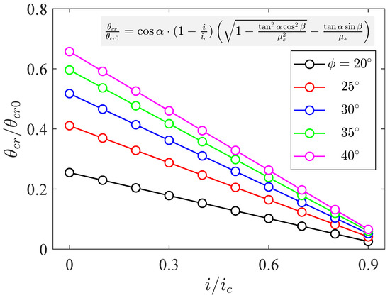
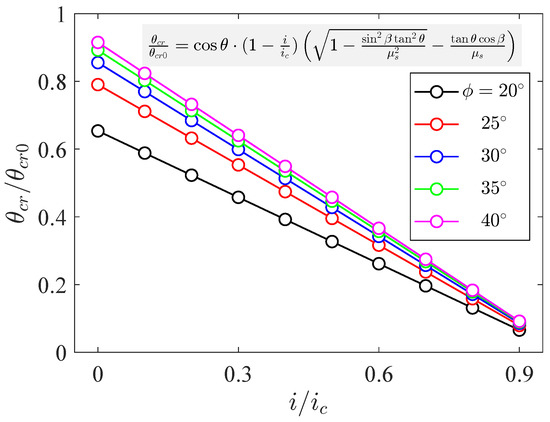
It is clear that the reduced Shields ratio ${\theta }_{cr}/{\theta }_{cr0}$ decreases linearly with the increase of seepage intensity. For transverse slopes, as shown in Figure 9, the reduced Shields ratio ${\theta }_{cr}/{\theta }_{cr0}$ decreases linearly with increasing seepage intensity under different slope angles. When the slope angle is zero, the case exactly degenerates into a flat seabed condition, and the maximum value is exactly equal to one. And, when the seepage intensity reaches a relatively large value, the Shields number considering seepage reduces to a relatively small value (<0.1) compared with the original Shields number on the flat bed. Meanwhile, under large seepage intensity, the effect of slope angle $\alpha$ is reduced. The results of longitudinal slopes are the same, as shown in Figure 10, except for the variation rate of ${\theta }_{cr}/{\theta }_{cr0}$ with the increased slope angle, where the results are consistent with Figure 4. Meanwhile, under each seepage intensity, the decreasing rate of ${\theta }_{cr}/{\theta }_{cr0}$ significantly increases with the larger slope angle. Under the same slope conditions, the change rate of ${\theta }_{cr}/{\theta }_{cr0}$ with $i/i_c$ is 38% to 42% lower than that of the transverse slope, and this change rate is negatively correlated with $\theta$, which is consistent with the results in Figure 4. Comparative analysis shows that, taking the ${15}^{\circ }$ slope as an example, the dynamic range of ${\theta }_{cr}/{\theta }_{cr0}$ of the longitudinal slope (0.087–0.872) is about 57% larger than that of the transverse slope (0.055–0.552), which confirms that the seepage–slope coupling effect has a stronger control on the sediment initiation of the longitudinal slope, that is, the seepage intensity under different slope gradients has a greater impact on the sediment initiation of the longitudinal slope.

Figure 9. Modified Shields number on a transverse slope with different seepage intensity ${\displaystyle \frac{i}{i_c}}$ and slope angle $\alpha$.

Figure 10. Modified Shields number on a longitudinal slope with different seepage intensity ${\displaystyle \frac{i}{i_c}}$ and slope angle $\theta$.

In addition, as shown in Figure 11, the incident wave angle could change under different seepage intensities with the transverse slope condition. The ${\theta }_{cr}/{\theta }_{cr0}$ decreases linearly under different incident wave angles. Due to the symmetrical distribution, only five typical incident current angles are selected ($0^{\circ }$, ${45}^{\circ }$, ${90}^{\circ }$, ${225}^{\circ }$, and ${270}^{\circ }$). Among different seepage intensities, the value of incident wave angle ${270}^{\circ }$ is the maximum and the value of ${90}^{\circ }$ is the minimum, which is consistent with the results of Figure 5. The variation magnitude between $0^{\circ }$ and ${45}^{\circ }$ is larger than the difference value between ${45}^{\circ }$ and ${90}^{\circ }$, which could also be seen in the sinusoidal variation pattern from Figure 5. Meanwhile, under large seepage intensity, the effect of incident wave angle $\beta$ is reduced. The incident wave angle changes under different seepage intensities with the longitudinal slope conditions are shown in Figure 12. Five typical incident current angles are selected ($0^{\circ }$, ${45}^{\circ }$, ${90}^{\circ }$, ${135}^{\circ }$, and ${180}^{\circ }$); the value of incident wave angle ${180}^{\circ }$ is the maximum, and the value of $0^{\circ }$ is the minimum, which is consistent with the result of Figure 6. By comparing the response characteristics of the seepage–inflow angle coupling effect of the two types of slopes, it can be seen that within the same seepage intensity range, the modified Shields number shows the same variation magnitude, indicating that the influence mechanism of seepage intensity on the initiation of sediment mobilization in the two types of slopes is inherently consistent.

Figure 11. Modified Shields number on a transverse slope with different seepage intensity ${\displaystyle \frac{i}{i_c}}$ and incident current angle $\beta$.

Figure 12. Modified Shields number on a longitudinal slope with different seepage intensity ${\displaystyle \frac{i}{i_c}}$ and incident current angle $\beta$.

As shown in Figure 13, the underwater response angle $\varphi$ could vary with different seepage intensities while the transverse slope conditions are considered. It is obvious that the reduced Shields ratio ${\theta }_{cr}/{\theta }_{cr0}$ increases with larger $\varphi$ non-linearly. Once the seepage intensity $i/i_c$ is determined, the growth rate of ${\theta }_{cr}/{\theta }_{cr0}$ is decelerating with the increase of $\varphi$, which is in line with Figure 7. Meanwhile, under large seepage intensity, the influencing effect of response angle $\varphi$ is reduced. The same calculation results for longitudinal slopes are depicted in Figure 14. The variation patterns are basically the same, except that ${\theta }_{cr}/{\theta }_{cr0}$ is larger for the longitudinal slope compared with the transverse slope under the same parameters. Comparative analysis shows that the modified Shields number of the longitudinal slope shows a more significant response amplitude in the process of seepage intensity change. Taking the ${30}^{\circ }$ response angle condition as an example, the dynamic range of ${\theta }_{cr}/{\theta }_{cr0}$ of the longitudinal slope (0.086–0.856) is about 65% larger than that of the transverse slope (0.052–0.518), which means that the seepage–response angle coupling effect has a stronger control effect on the sediment initiation of the longitudinal slope, that is, the seepage intensity under different response angles has a greater impact on the sediment initiation on the longitudinal slope.

Figure 13. Modified Shields number on a transverse slope with different seepage intensity ${\displaystyle \frac{i}{i_c}}$ and soil angle of response $\varphi$.

Figure 14. Modified Shields number on a longitudinal slope with different seepage intensity ${\displaystyle \frac{i}{i_c}}$ and soil angle of response $\varphi$.

4. Collaborative Calculation of Four Slope Parameters with Two Slope Conditions

In this section, the four aforementioned parameters (slope ratio, incident current angle, soil angle of response, and vertical seepage intensity) within two slope types are systematically calculated to obtain the influence on the modified Shields ratio. The incident current angle ranges from $0^{\circ }$ to ${360}^{\circ }$, which means the current and drag force could act on the particle in all directions on the slope. The soil angle of response ranges from ${20}^{\circ }$ to ${40}^{\circ }$, which is the common range of the response angles of quaternary non-cohesive sediments. The slope ratios are set as $0^{\circ }$, ${15}^{\circ }$, and ${30}^{\circ }$, and the seepage intensities are set as 0.1, 0.5, and 0.9. In order to display the calculation results more intuitively, the results of contour plots are depicted.

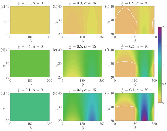
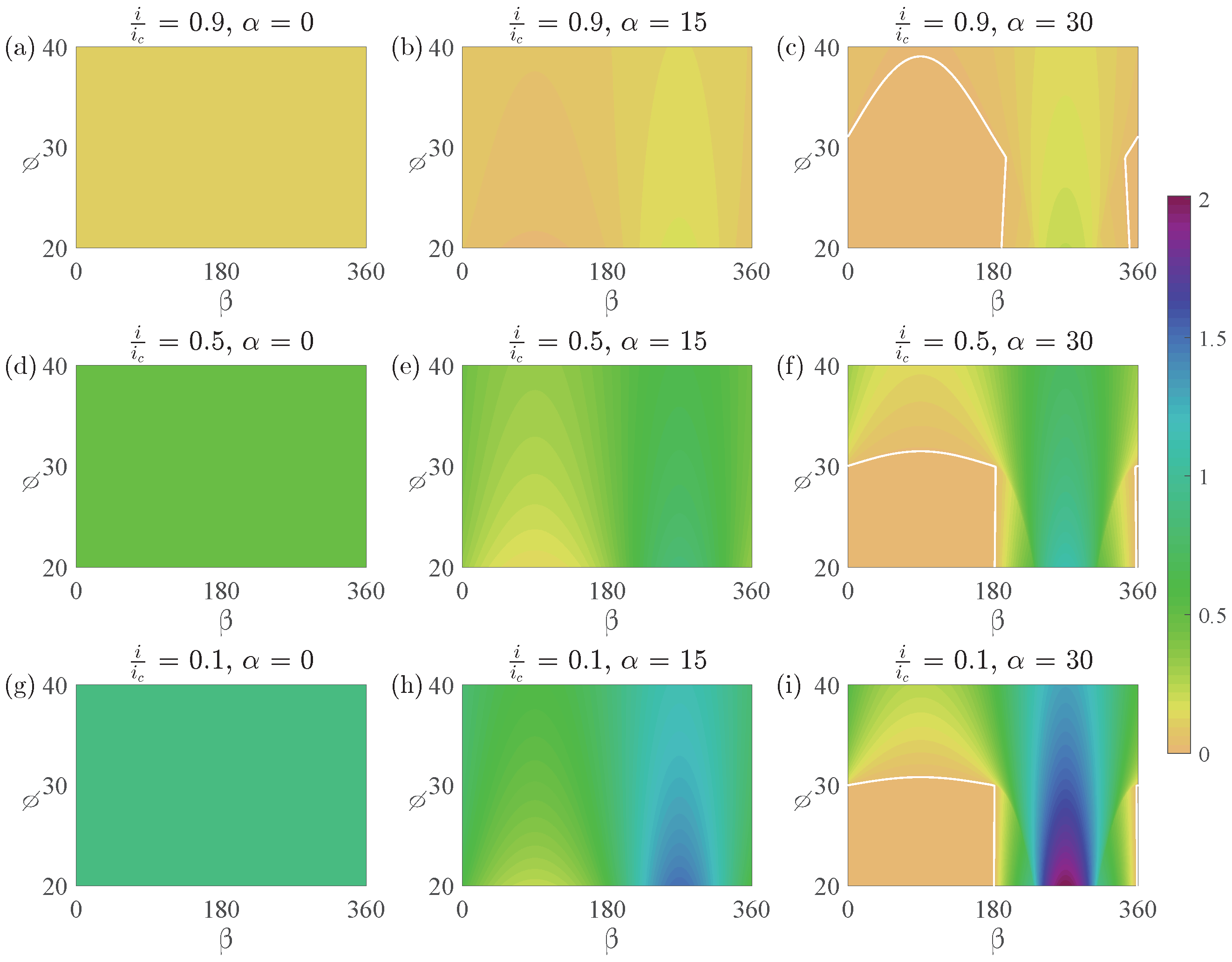
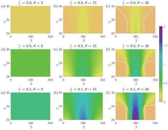
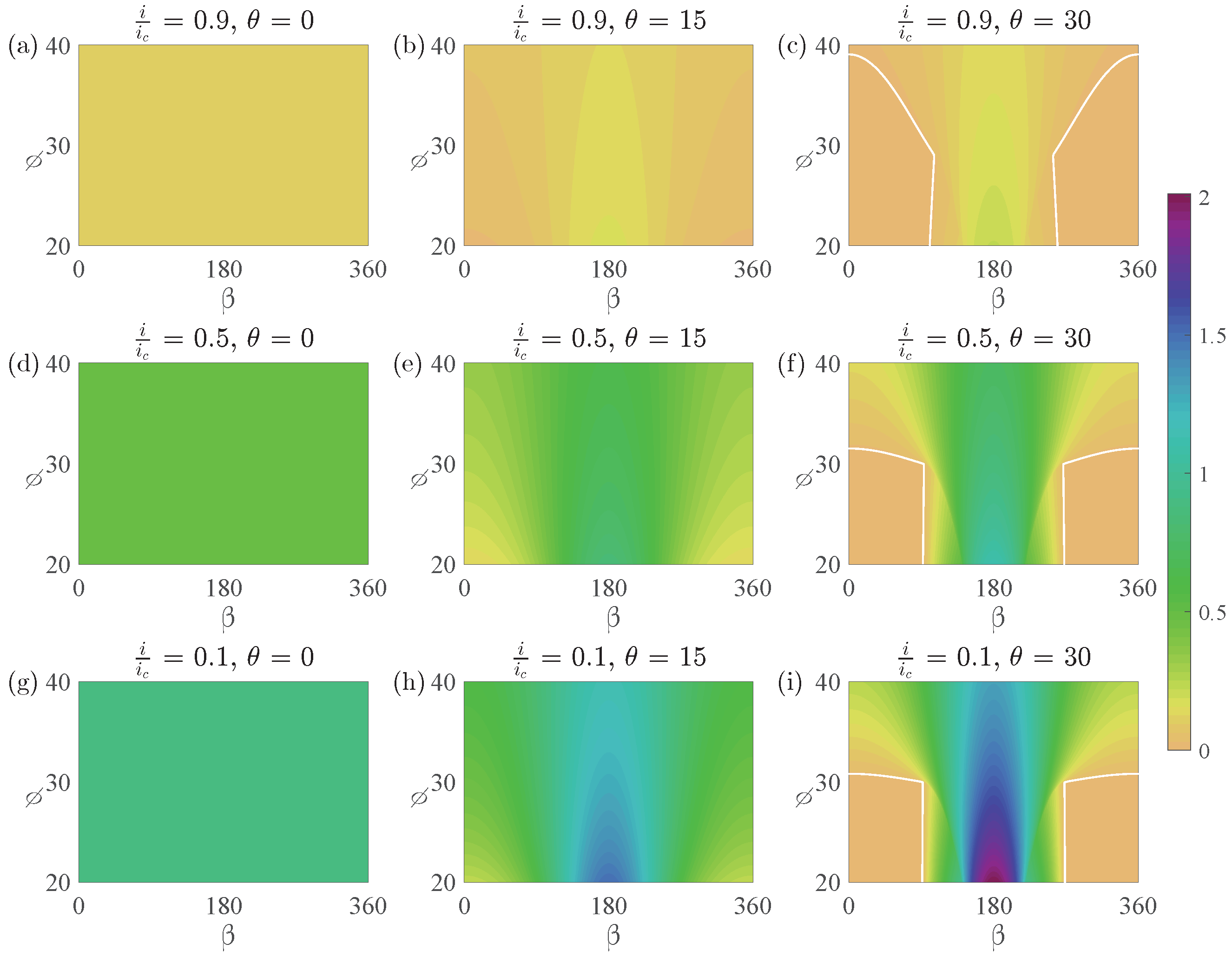
For the transverse slope condition ($\theta$ = 0), the results are shown in Figure 15. Three seepage intensities and three slope angles make up nine cases within the above-mentioned incident current ranges and slope response angle conditions. The first column is the flat bed condition ($\alpha$ = 0), and the value of ${\theta }_{cr}/{\theta }_{cr0}$ is constant in the fields; from top to bottom the results are 0.1, 0.5 and 0.9, respectively, exactly equal to the values of $1-{\displaystyle \frac{i}{i_c}}$. The second column is the small slope condition ($\alpha$ = ${15}^{\circ }$); it is clear that under large seepage intensity (such as Figure 15b, $i/i_c$ = 0.9), the results of ${\theta }_{cr}/{\theta }_{cr0}$ are much reduced, as the values are nearly 0. When the seepage is small (such as Figure 15h, $i/i_c$ = 0.1), it is obvious that the value of ${\theta }_{cr}/{\theta }_{cr0}$ is reduced with the incident current angle ranges from $0^{\circ }$ to ${90}^{\circ }$ and ${270}^{\circ }$ to ${360}^{\circ }$ (${\theta }_{cr}/{\theta }_{cr0}⩽$ 1), while it is increased within the range of ${90}^{\circ }$ to ${270}^{\circ }$ (${\theta }_{cr}/{\theta }_{cr0}⩾$ 1).

Figure 15. 2D modified Shields number contours for a transverse slope. (a–c) ${\displaystyle \frac{i}{i_c}}=0.9$, $\alpha =0^{\circ },{15}^{\circ },{30}^{\circ }$; (d–f) ${\displaystyle \frac{i}{i_c}}=0.5$, $\alpha =0^{\circ },{15}^{\circ },{30}^{\circ }$; (g–i) ${\displaystyle \frac{i}{i_c}}=0.1$, $\alpha =0^{\circ },{15}^{\circ },{30}^{\circ }$.

Furthermore, with the increase of response angle $\varphi$, the value of ${\theta }_{cr}/{\theta }_{cr0}$ varies with different incident angles; the result increases with the response angle $\varphi$ that ranges from $0^{\circ }$ to ${180}^{\circ }$, while it decreases with the response angle $\varphi$ that ranges from ${180}^{\circ }$ to ${360}^{\circ }$. The third column is the large slope condition ($\alpha$ = ${30}^{\circ }$); we note that within the range of $0^{\circ }$ to ${180}^{\circ }$, ${\theta }_{cr}/{\theta }_{cr0}$ decreases with the increase of slope angle (${15}^{\circ }$ to ${30}^{\circ }$), while ${\theta }_{cr}/{\theta }_{cr0}$ increases with the increase of slope angle within the range of ${180}^{\circ }$ to ${360}^{\circ }$.

Meanwhile, it is worth noting that within the range of $0^{\circ }$ to ${180}^{\circ }$, there exists a nearly zero ${\theta }_{cr}/{\theta }_{cr0}$ field around the response angle of ${20}^{\circ }$ to ${30}^{\circ }$ (e.g., ${\theta }_{cr}/{\theta }_{cr0}⩽0.025$). This is because when the soil angle of response is no larger than the slope, the sand particle could move under its gravity force without any drag force. Furthermore, the initiation condition is weakened under the action of seepage; therefore, a wider range of initiation occurs easily under weak hydrodynamic conditions. For example, under a downward slope current ($\beta$ ranges $0^{\circ }$ to ${180}^{\circ }$, see Figure 2a) or even a small angle upward slope current ($\beta$ is close to ${180}^{\circ }$ or ${360}^{\circ }$), the sand can easily move. Meanwhile, when the seepage intensity is increased, the nearly zero ${\theta }_{cr}/{\theta }_{cr0}$ field becomes larger, as shown by the white solid line in the Figure 15c,f,i. The non-linear effects of various flow directions and seepage sizes on the incipient motion of sediment are primarily highlighted here.

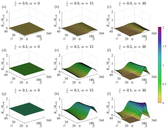
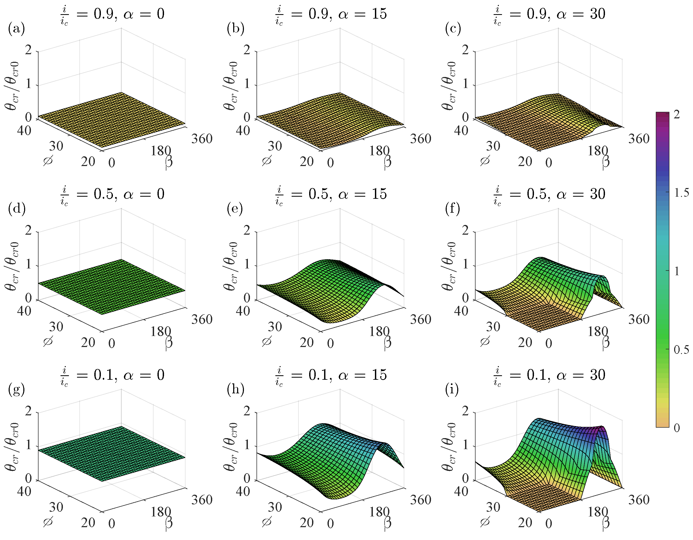
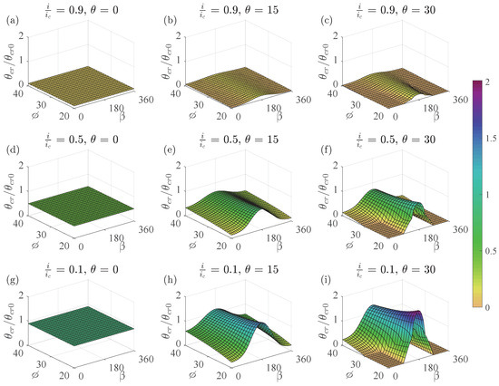
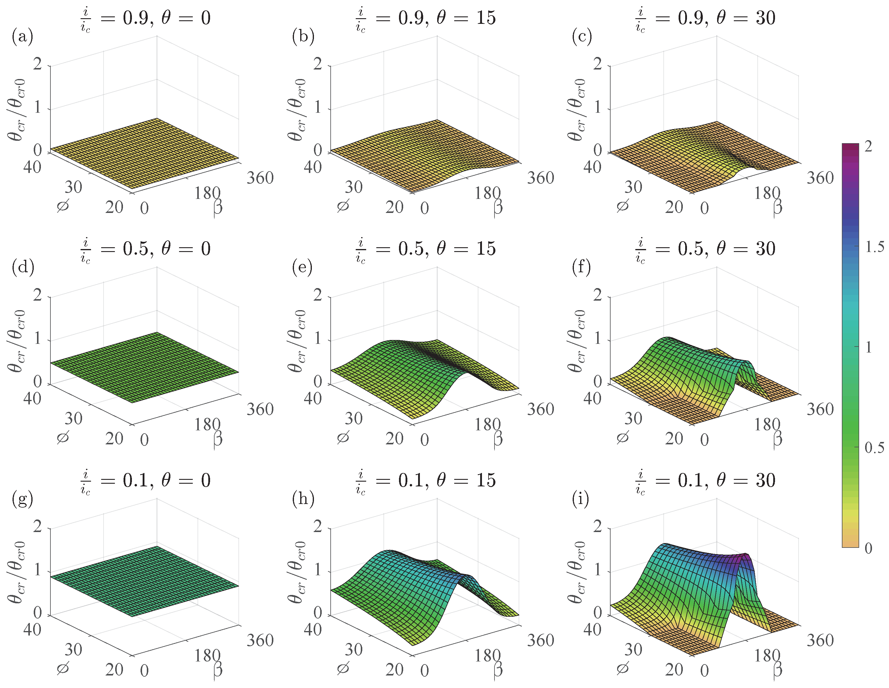
Through uniformly meshed operation, the three-dimensional (3D) contours of modified Shields number are shown in Figure 16, in which the above-mentioned characteristics are significant and more intuitive.

Figure 16. 3D meshed modified Shields number contours for a transverse slope. (a–c) ${\displaystyle \frac{i}{i_c}}=0.9$, $\alpha =0^{\circ },{15}^{\circ },{30}^{\circ }$; (d–f) ${\displaystyle \frac{i}{i_c}}=0.5$, $\alpha =0^{\circ },{15}^{\circ },{30}^{\circ }$; (g–i) ${\displaystyle \frac{i}{i_c}}=0.1$, $\alpha =0^{\circ },{15}^{\circ },{30}^{\circ }$.

For the longitudinal slope condition ($\alpha$ = 0), the results are shown in Figure 17. Three seepage intensities and three slope angles make up nine cases within the above-mentioned incident current ranges and slope response angle ranges.

Figure 17. 2D Modified Shields number contours for a longitudinal slope. (a–c) ${\displaystyle \frac{i}{i_c}}=0.9$, $\theta =0^{\circ },{15}^{\circ },{30}^{\circ }$; (d–f) ${\displaystyle \frac{i}{i_c}}=0.5$, $\theta =0^{\circ },{15}^{\circ },{30}^{\circ }$; (g–i) ${\displaystyle \frac{i}{i_c}}=0.1$, $\theta =0^{\circ },{15}^{\circ },{30}^{\circ }$.

The first column is the flat bed conditions ($\beta$ = 0), and the value of ${\theta }_{cr}/{\theta }_{cr0}$ remains constant in the fields; from top to bottom the results are 0.1, 0.5 and 0.9, respectively, exactly equal to the values of $1-{\displaystyle \frac{i}{i_c}}$. The second column is the small slope condition ($\alpha$ = ${15}^{\circ }$); it is clear that under large seepage intensity (such as Figure 17b, $i/i_c$ = 0.9), the results of ${\theta }_{cr}/{\theta }_{cr0}$ are much reduced; the values are nearly zero, except for the values in the vicinity of ${180}^{\circ }$ incident current angle. When the seepage is small (such as Figure 17h, $i/i_c$ = 0.1), it is obvious that the value of ${\theta }_{cr}/{\theta }_{cr0}$ is increased within the incident current angle of $0^{\circ }$ to ${180}^{\circ }$ (${\theta }_{cr}/{\theta }_{cr0}⩽$ 1), while it is reduced within the range of ${180}^{\circ }$ to ${360}^{\circ }$ (${\theta }_{cr}/{\theta }_{cr0}⩾$ 1).

Furthermore, with the increase of response angle $\varphi$, the value of ${\theta }_{cr}/{\theta }_{cr0}$ varies with different incident angles; the result increases with the response angle $\varphi$ ranging from $0^{\circ }$ to ${90}^{\circ }$ and ${270}^{\circ }$ to ${360}^{\circ }$, while it decreases with the response angle $\varphi$ ranging from ${90}^{\circ }$ to ${270}^{\circ }$. The third column is the large slope condition ($\alpha$ = ${30}^{\circ }$); it is noteworthy that within the range of $0^{\circ }$ to ${90}^{\circ }$, and ${270}^{\circ }$ to ${360}^{\circ }$, ${\theta }_{cr}/{\theta }_{cr0}$ decreases with the increase of slope angle (${15}^{\circ }$ to ${30}^{\circ }$), while ${\theta }_{cr}/{\theta }_{cr0}$ increases with the increase of slope angle within the range of ${90}^{\circ }$ to ${270}^{\circ }$.

Meanwhile, it is worth noting that within the range of $0^{\circ }$ to ${90}^{\circ }$ and ${270}^{\circ }$ to ${360}^{\circ }$, there exists a nearly zero ${\theta }_{cr}/{\theta }_{cr0}$ field around the response angle of ${20}^{\circ }$ to ${30}^{\circ }$, because when the soil angle of response is no larger than the slope, the sand particle could move under its gravity force without any drag force. In addition, a wider range of initiation occurs easily under weak hydrodynamic conditions due to the seepage effect. For instance, under a downward slope current ($\beta$ ranges $0^{\circ }$ to ${90}^{\circ }$ and ${270}^{\circ }$ to ${360}^{\circ }$, see Figure 2b) or even a small angle upward slope current ($\beta$ is close to ${180}^{\circ }$ or ${360}^{\circ }$), the sediment initiation easily occurs. Meanwhile, when the seepage intensity is increased, the non-linear interaction of flow direction and seepage intensity causes the nearly zero ${\theta }_{cr}/{\theta }_{cr0}$ field to become larger, as shown by the white solid line in the Figure 18c,f,i. The three-dimensional (3D) contours of the modified Shields number are illustrated in Figure 18 through meshed treatment, where the aforementioned characteristics are clear and more intuitive.

Figure 18. 3D meshed modified Shields number contours for a longitudinal slope. (a–c) ${\displaystyle \frac{i}{i_c}}=0.9$, $\theta =0^{\circ },{15}^{\circ },{30}^{\circ }$; (d–f) ${\displaystyle \frac{i}{i_c}}=0.5$, $\theta =0^{\circ },{15}^{\circ },{30}^{\circ }$; (g–i) ${\displaystyle \frac{i}{i_c}}=0.1$, $\theta =0^{\circ },{15}^{\circ },{30}^{\circ }$.

5. Numerical Simulation and Verification

The scour model adopted here is ibScourFoam, which is an open source code implemented in OpenFOAM version 5.x, and the immersed boundary method is embedded, which is more suitable for complex boundary fluid–solid coupling problems. The seepage result distributions are obtained through a wave–structure–seabed (WSSI) model, which is also implemented in the OpenFOAM platform. Through the combination of the scour model and WSSI model, the scour results considering vertical seepage could be obtained.

5.1. Hydrodynamic Model

Firstly, in the hydrodynamic model, the RANS equation and the $k-\omega$ SST-SAS model for turbulence is included., and the immersed boundary method and the near-wall function are introduced.

The 3D incompressible Reynolds-Averaged Navier–Stokes equations are written as:

$$\begin{array}{cc}\hfill \nabla ·\mathbf{u}& =0\hfill \\ \hfill {\displaystyle \frac{\partial \mathbf{u}}{\partial t}}+\nabla ·\left(\mathbf{u}\mathbf{u}\right)& =-{\displaystyle \frac{\nabla p}{\rho }}+\nabla ·\left[\left(v+v_t\right)\nabla \mathbf{u}\right]\hfill \end{array}$$

(15)

where u is the Reynolds-averaged flow velocity, p is the mean pressure, $\rho$ is water density, $\nu$ is kinematic viscosity, and ${\nu }_t$ denotes the eddy viscosity.

The $k-\omega$ model has been proven to achieve better simulation capabilities in the near-wall area and numerical stability [39]. In this simulation, the $k-\omega$ SST-SAS model [40] is adopted and its governing equations are:

$$\begin{array}{cc}\hfill {\displaystyle \frac{\partial k}{\partial t}}+\nabla ·\left(\mathbf{u}k\right)=& \nabla ·\left[\left(\nu +{\alpha }_k{\nu }_t\right)\nabla k\right]+P_k-C_{\mu }k\omega \hfill \\ \hfill {\displaystyle \frac{\partial \omega }{\partial t}}+\nabla ·\left(\mathbf{u}\omega \right)=& \nabla ·\left[\left(\nu +{\alpha }_{\omega }{\nu }_t\right)\nabla \omega \right]+\alpha {\displaystyle \frac{\omega }{k}}{P}_k-\beta {\omega }^2\hfill \\ \hfill & +{\displaystyle \frac{2}{{\alpha }_{\omega 2}}}\left(1-F_1\right){\displaystyle \frac{1}{\omega }}\nabla k\nabla \omega +Q_{SAS}\hfill \end{array}$$

(16)

where k denotes the turbulence kinetic energy and $\omega$ denotes the specific dissipation rate. $P_k={\nu }_t{\mathbf{S}}^2$ is the production term, $\mathbf{S}=\sqrt{2{\mathbf{S}}_{ij}{\mathbf{S}}_{ij}}$ is a scalar invariant of the strain rate tensor ${\mathbf{S}}_{ij}=0.5[{(\nabla \mathbf{u})}_{ij}+{(\nabla \mathbf{u})}_{ij}]$.

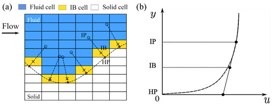
The immersed boundary method includes three cell types based on their relative position to the immersed bed surface: (1) the first cell type that intersects with the immersed boundary, having their centers positioned on the fluid side, is recognized as IB cells; (2) the cells that are entirely on the fluid side are designated as fluid cells; and (3) the cells with centers located on the solid (sediment) side are referred to as solid cells. The flow variables only need to be solved for those fluid cells, while the flow variables of solid cells are set at zero. For the IB cells, the flow variables are determined based on a wall model.

In the wall model, three distinct point types are defined in the near-wall region, as illustrated in Figure 19. The first point is the IB cell center; the second is the image point (IP) located on the normal line to the immersed boundary that intersects the IB cell center; the third is the hit point (HP), where the normal line intersects the immersed boundary. The flow values at the IPs are interpolated from the neighboring cells.

Figure 19. Mesh generation near immersed boundary and velocity profile. (a) Three point types in the near-wall region; (b) velocity profile.

The distance between an IP and the immersed boundary $d_{IP}$ is set to three times the minimum length of the IB cell $l_{\ast }$. Around the bed surface, because the cells are uniform and similarly sized, the mentioned distance $d_{IP}$ is almost uniform. The wall function in the IB method is as follows. It is assumed that an IP and the center of its corresponding IB cell are located on the same log-law velocity profile, which can be expressed as:

$$u^{+}={\displaystyle \frac{1}{\kappa }}ln\left(E^{\prime }{y}^{+}\right)$$

(17)

where $u^{+}=u/u_{\tau }$ and $y^{+}=y{u}_{\tau }/\nu$ are the dimensionless velocity and wall distance, respectively. The shear velocity $u_{\tau }$ is related with wall shear stress as $\tau =\rho u_{\tau }^2$. $E^{\prime }$ is a wall roughness parameter related to boundary roughness.

Therefore, with an interpolated velocity at an IP, $u_{IP}$ and the distance $d_{IP}$, the log-law distribution is written as:

$${\displaystyle \frac{u_{IP}}{u_{\tau }}}={\displaystyle \frac{u_{IP}}{y_{IP}^{+}\nu /y}}={\displaystyle \frac{1}{\kappa }}ln\left(E^{\prime }{y}_{IP}^{+}\right)$$

(18)

Through Newton–Raphson iteration, $y_{IP}^{+}$ could be solved iteratively using the following equation:

$$y_{IP,i+1}^{+}={\displaystyle \frac{y_{IP,i}^{+}+\kappa y{u}_{IP}/\nu }{1+ln\left(E^{\prime }{y}_{IP,i}^{+}\right)}}$$

(19)

Hereafter, the shear velocity $u_{\tau }$ could be determined through the definition of $y_{IP}^{+}$.

Another important issue is the velocity profile between the IB cell center and the immersed bed boundary. The log-law profile could induce numerical instability if the distance $y_{IB}$ is too small, although the IB cell may indeed be located within the log-law layer. To solve this problem, a linear velocity distribution between the IP and HP is assumed in order to estimate the velocity at the IB, as shown in Figure 19. The slope of the linear profile is assumed to be equal to the slope of the log-law profile at the IP. To maintain the same value of the shear stress on the immersed boundary, the eddy viscosity is kept constant between IP and HP ($u_{\tau }^2=(\nu +{\nu }_t)\partial u/\partial y$). The advantage of this method is that this approach prevents the discontinuous behavior that arises from using different wall functions in the laminar sublayer and the log-law layer.

Based on the linear assumption described above, the tangential velocity $u_{IB,tan}$ and the normal velocity $u_{IB,norm}$ at the IB cell center is measured as:

$$\begin{array}{cc}\hfill & u_{IB,tan}=u_{IP,tan}-{\left({\displaystyle \frac{\partial u^{+}}{\partial y^{+}}}\right)}_{IP,tan}(y_{IP}-y_{IB})u_{\tau }\hfill \\ \hfill & u_{IB,norm}=u_{IB,norm}{\displaystyle \frac{d_{IP}}{d_{IB}}}\hfill \end{array}$$

(20)

where $\partial u^{+}/\partial y^{+}=1/\left(\kappa y^{+}\right)$.

The turbulence kinetic energy, $k=u_{\tau }^2/\sqrt{C_{\mu }}$, is nearly constant in the near-wall region [41]. The eddy viscosity ${\nu }_t=k/\omega$ is also approximately constant between the IP and IB cell centers to maintain smooth shear stress variation [42]. ${\omega }_{IB}$ is expressed as:

$${\omega }_{IB}={\omega }_{IP}=\sqrt{{\omega }_{vis}^2+{\omega }_{log}^2}=\sqrt{{\left({\displaystyle \frac{6.0\nu }{0.075y_{IP}^2}}\right)}^2+{\left({\displaystyle \frac{k^{1/2}}{C_{\mu }^{1/4}\kappa y_{IP}}}\right)}^2}$$

(21)

5.2. Bed Morphodynamic Model

In this section, the morphodynamic model is introduced, in which the bed-load transportation is considered. The morphodynamics is implemented through an unstructured triangular mesh, which is adopted as the immersed boundary for the flow solver. The bed-load transport rate for a flat horizontal bed is solved through the empirical formula proposed by [35],

$${\displaystyle \frac{q_0}{\sqrt{Rgd}d}}=\left\{\begin{array}{cc}18.74\left(\theta -{\theta }_c\right)\left({\theta }^{1/2}-0.7{\theta }_c^{1/2}\right),\hfill & \mathrm{if}\theta >{\theta }_c\hfill \\ 0,\hfill & \mathrm{if}\theta <{\theta }_c\hfill \end{array}\right.$$

(22)

where R is the submerged specific gravity, usually 1.65 for quartz sand, d is the sediment grain size, $\theta =\left|\tau \right|/\left(\rho gRd\right)$ is the Shields number, and ${\theta }_c$ is the critical Shields number, which could be calculated from the modified fit to the Shields diagram [43],

$${\theta }_{c0}=0.5\times \left(0.22\times R{e}_p^{-0.6}+0.06\times {10}^{-7.7R{e}_p^{-0.6}}\right)$$

(23)

For the local bed slope and local in-flow direction, the critical Shields number could be defined by Equation (14).

The evolution of the bed elevation is determined by the Exner equation,

$$(1-n){\displaystyle \frac{\partial z_b}{\partial t}}=-\nabla ·\left(q_0{\displaystyle \frac{\tau }{\left|\tau \right|}}\right)$$

(24)

where $z_b$ is the bed elevation and n is the porosity of bed.

It should be noted that the Exner equation only considers the conservation of mass for bed sediment. It does not consider other factors such as the stability of the granular bed if the angle exceeds the angle of repose. The sand slide model is considered to re-correct this problem. The sand slide model is based on the slope-limited diffusion method, according to Fick’s law of diffusion,

$$\begin{array}{cc}\hfill \mathbf{q}=-& K\nabla z_b\hfill \\ \hfill {\displaystyle \frac{\partial z_b}{\partial t}}=& K{\nabla }^2{z}_b\hfill \end{array}$$

(25)

where $\mathbf{q}$ is sand slide flux, K is sand slide diffusivity ($L^2/T$), and the sediment diffusive flux must satisfy the mass conservation.

In the context of sand slide, one deviation from Fick’s law is that the flux is limited by the bed slope. If the bed angle is less than or equal to the angle of repose, there is no sand slide and flux should be zero. To reflect this, the diffusivity K should be a conditional function as follows:

$$K=\left\{\begin{array}{cc}{K}_0,\hfill & \mathrm{if}\left|\nabla z_b\right|\ge tan{\varphi }_0\hfill \\ 0,\hfill & \mathrm{otherwise}\hfill \end{array}\right.$$

(26)

where $K_0$ is the diffusivity coefficient once sand slide initiates and forms a constant value. The detailed information about diffusion coefficient determination and numerical schemes can be found in the work by Song et al. [44].

5.3. Scheme and Validation

In this section, the scour experiment conducted by Roulund et al. [38] is compared with the simulation. The flow resistance estimator in Chen et al. [45] was used to estimate the roughness height, and the shear velocity measured in the flume experiment was adopted. The flow condition and sediment properties are shown in Table 2; case 1 and case 2 are hydrodynamic and scour verification, respectively.

Table 2. Scour model validation and parameter settings.

	Parameter	Symbol	Value (Unit)
Case 1: Smooth bed mono-pile hydraulic comparison	water depth	d	54 (cm)
	cross-section average velocity	V	32.6 (cm/s)
	pile diameter	D	53.6 (cm)
	roughness height	$k_s$	0 (cm)
Case 2: Mono-pile scour comparison	water depth	d	40 (cm)
	cross-section average velocity	V	46 (cm/s)
	pile diameter	D	10 (cm)
	roughness height	$k_s$	0.5 (cm)
	grain size	$d_{50}$	0.26 (mm)
	critical Shields number of flat bed	$\theta$	0.022 (-)
	static friction coefficient	${\mu }_s$	0.63 (-)
	shear velocity	$u_{\tau }$	2.8 (cm/s)

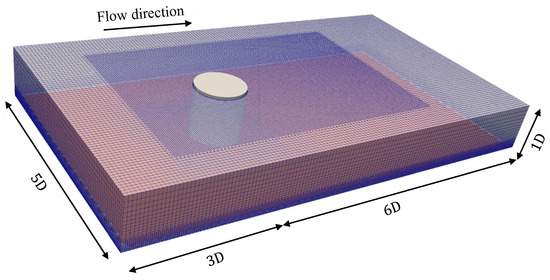
In the flow part, the mesh design is depicted in Figure 20; the size of the flow field area is set to be 9D in length, 5D in width and 1D in height (D is the diameter of the single pile), and the mesh refinement is performed in the area around the single pile, especially for the downstream area behind the pile, so as to capture the flow field change on the downstream side of the mono-pile more accurately. The simulation process consists of two stages. In the first stage, it runs for 300 s to establish a stable flow state. Based on the average flow velocity during this time, it is estimated that the volume of fluid flowing through the computational domain is approximately 20 times the volume of the domain itself. Subsequently a continuous simulation lasting 100 s was conducted to collect time-history data of the flow field parameters. The average flow field variables were then calculated and compared with experimental data from Roulund et al. [38].

Figure 20. Mesh generation for flow around circular pile on smooth bed (blue mesh and red bed).

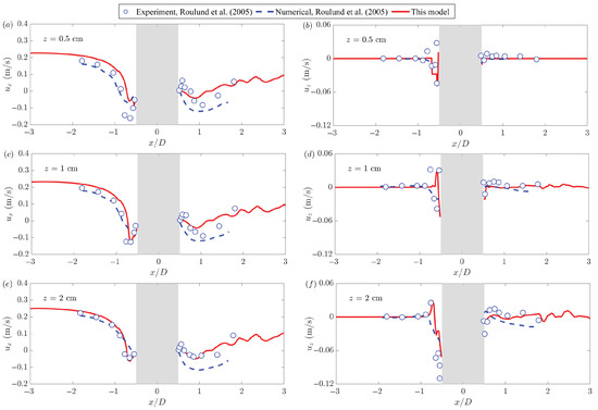
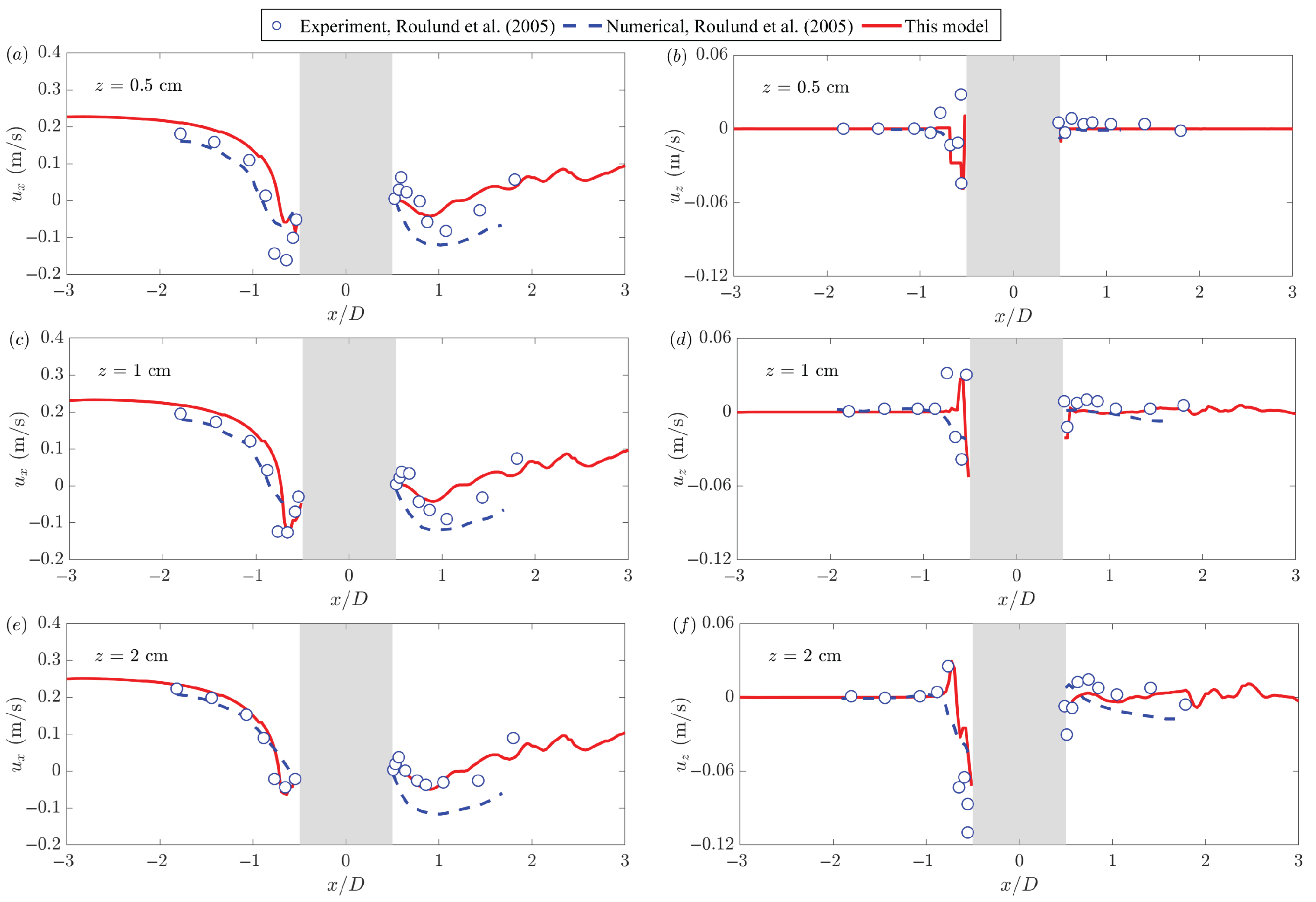
Figure 21 illustrates the comparison of time-averaged flow velocities $u_x$ and $u_z$ at various heights (z = 0.5, 1, and 2 cm) on the plane of symmetry ($y=0$). The red curve represents the numerical simulation results from this study, while the blue dashed line and blue hollow circle indicate the numerical simulation and measured data from Roulund et al. [38], respectively. The average flow velocity was monitored at three vertical locations (z = 0.5, 1, and 2 cm). The left column of the figure displays the flow velocity distribution in the x-direction. The downward flow caused by the horseshoe vortex on the upstream surface of the pile results in a negative x-direction velocity, which indicates a flow direction upstream. This reverse velocity leads to erosion and scouring at the tip of the pile, as sediment particles are carried by the upper mainstream to the area behind the pile. As the height (z) increases, the effect of the horseshoe vortex weakens, causing a corresponding decrease in the amplitude of the negative flow velocity. The right column of the figure illustrates the velocity distribution in the z-direction. The velocity fluctuations observed upstream of the pile confirm the presence of the water-blocking effect and the associated downward flow. In contrast, the downstream area displays randomness due to the shedding of the wake vortex. After averaging, the velocities in both the x and z directions exhibit an oscillating trend along the path (from $x/D$ = 0.5 to 3). A comprehensive comparison indicates that the numerical model aligns closely with the experimental data, effectively replicating the dynamic characteristics of the flow field around the pile.

Figure 21. Validation of velocity distribution along flow direction at different depths against Roulund et al. [38]. (a) $z=0.5$ cm, $u_x$; (b) $z=0.5$ cm, $u_z$; (c) $z=1$ cm, $u_x$; (d) $z=1$ cm, $u_z$; (e) $z=2$ cm, $u_x$; (f) $z=2$ cm, $u_z$.

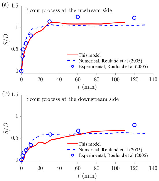
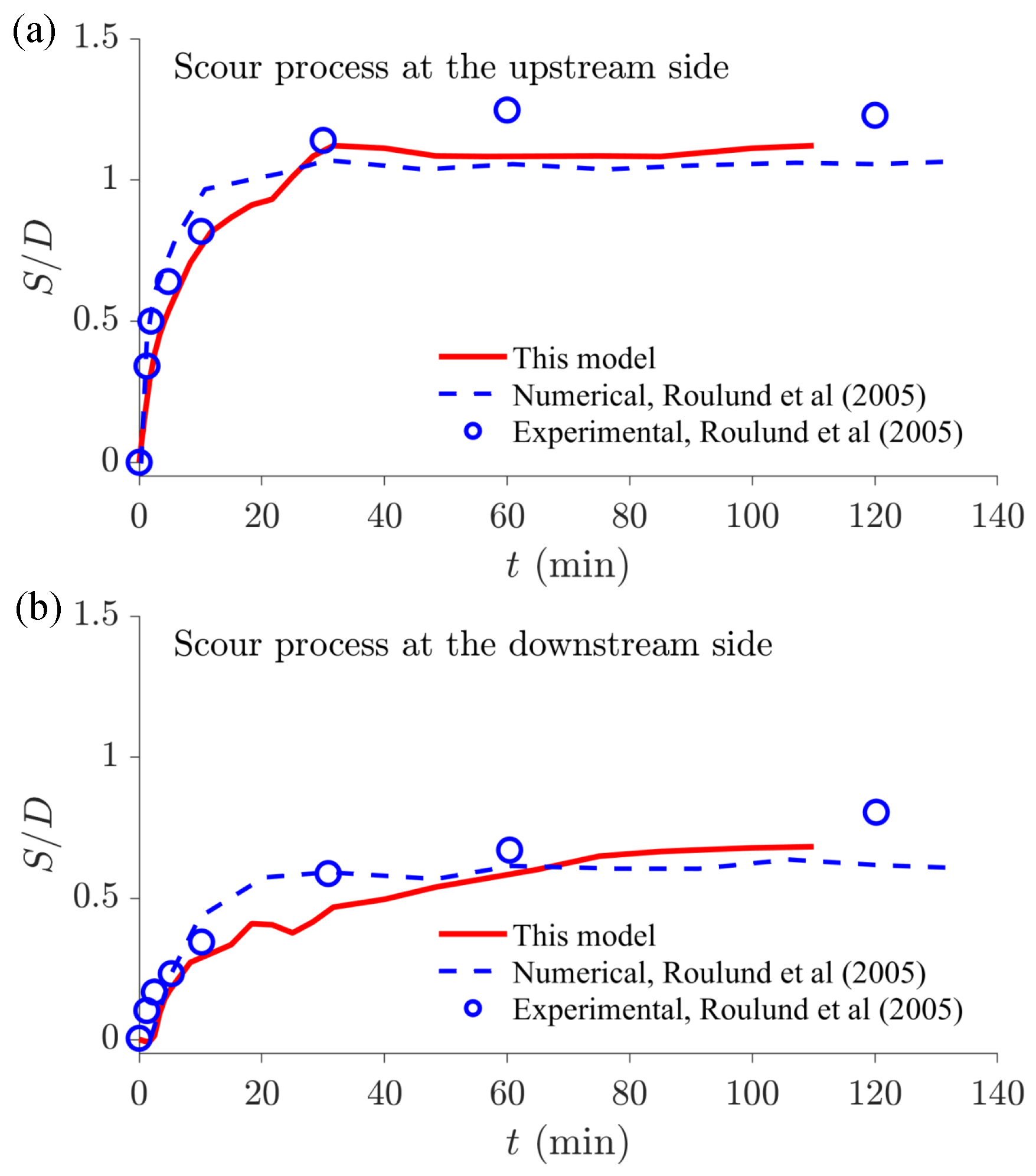
Moreover, in the scour result of case 2, the scour depth development curves are compared with simulation results; the upstream and downstream results are both included. The result of the upstream side is shown in Figure 22a; the scour depths of both upstream and downstream sides of the pile increase quickly in the first 0.5 h and then develop gently. The scour depth at the upstream side of the cylinder almost reaches its equilibrium earlier than that at the downstream side in the experimental condition. At the upstream side, the predicted maximum scour depths in Roulund et al. [38] and this simulation are 1.06 D and 1.12 D, respectively. The measured maximum scour depth from the experiment is 1.25 D. The simulation scour depth result compares well with the experiment, with a tolerance of 10%.

Figure 22. Comparative validation of temporal scour depth evolution around mono-pile against Roulund et al. [38]. (a) Scour process at the upstream side; (b) scour process at the downstream side.

The result of the downstream side is shown in Figure 22b; at the downstream side, there exists a scour lag around 2 min, which is also obvious in the numerical result of Roulund et al. [38]. The simulations in Roulund et al. [38] and this research give the maximum values equal to 0.64 D and 0.68 D. The measured maximum scour depth from the experiment is 0.80 D. The simulation scour depth result compares well with the experiment, with a tolerance of 15%, a bit larger than the upstream side results.

More importantly, the influence of vertical seepage on scour should be verified. The calculation process of seepage intensity ($i/i_c$) should be briefly described. The underwater weight of one single sand particle is expressed as $W^{\prime }$,

$$W^{\prime }=\left({\gamma }_s-{\gamma }_w\right){\displaystyle \frac{\pi d_{50}^3}{6}}$$

(27)

where ${\gamma }_s$ and ${\gamma }_w$ are the weight of sand sediment and water and $d_{50}$ is the median particle size of sediment particles.

Meanwhile, the seepage force per unit volume acting on porous media soil can be expressed as S [33],

$$S={\displaystyle \frac{\partial \overrightarrow{p}}{\partial \overrightarrow{h}}}$$

(28)

where $\partial \overrightarrow{h}$ is the action direction of the seepage force; in the research, this is the vertical direction.

Considering the uniform distribution of sediment particles in space, the number of sediment particles per unit volume is expressed as N [46],

$$N={\displaystyle \frac{1-n}{\pi d_{50}^3/6}}$$

(29)

where n is the porosity of sand sediment.

Therefore, the seepage force acting on a sand particle is $S/N$; the acting direction is reverse to the result in Equation (28). The seepage force acting vertically is expressed as,

$$F_{sz}=-{\displaystyle \frac{\partial p}{\partial z}}·{\displaystyle \frac{\pi d_{50}^3}{6\left(1-n\right)}}$$

(30)

where $(1-n)$ denotes the converted unit seepage force after considering the porosity of the sand–water mixture.

Finally, $i/i_c$ is equal to $F_{sz}/W^{\prime }$. When the value is 1, the sand particle is in a complete state of suspension. $i/i_c$ is expressed as,

$${\displaystyle \frac{i}{i_c}}=-{\displaystyle \frac{\partial p}{\partial z}}·{\displaystyle \frac{1}{(1-n)({\gamma }_s-{\gamma }_w)}}$$

(31)

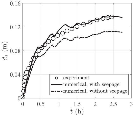
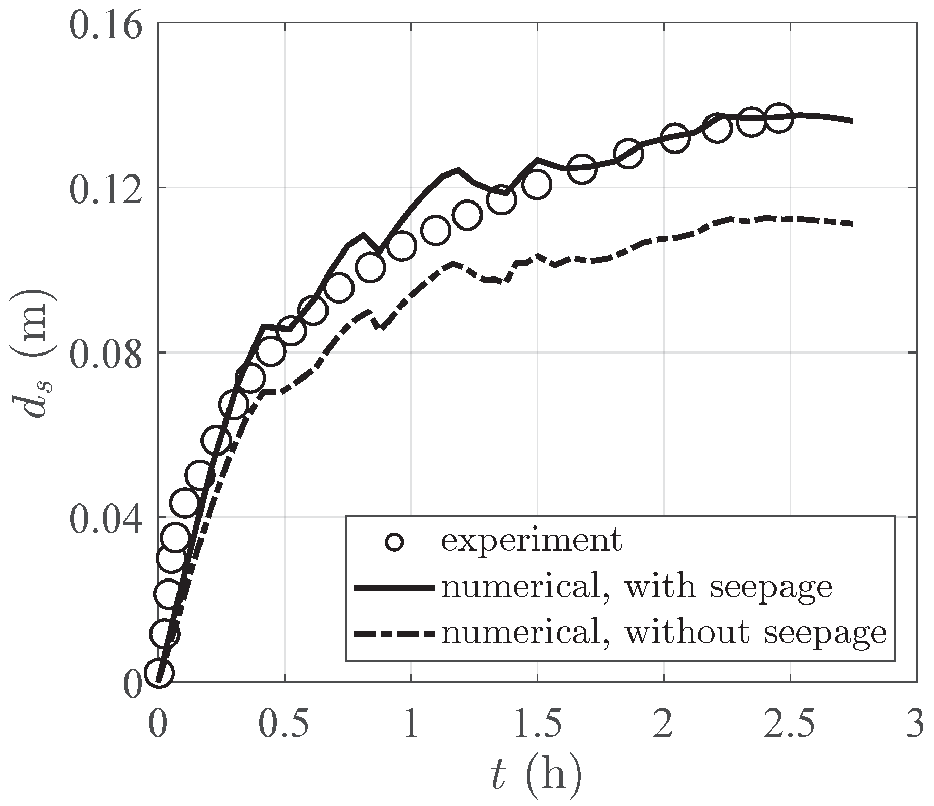
In addition, the mono-pile scouring experiment conducted by Qi and Gao [22] is compared. The influence of the vertical seepage effect of the numerical model on scour calculation is verified. The sand particle size is 0.38 mm and the seepage coefficient is $1.88\times {10}^{-4}$ m/s. The void ratio and relative density are 0.771 and 0.352, respectively. Wave-current loading (condition 8) is adopted; the water depth is $0.5\mathrm{m}$, pile diameter is $0.2\mathrm{m}$, wave height is $0.085\mathrm{m}$, wave period is $1.4\mathrm{s}$, and current velocity is $0.23\mathrm{m}/\mathrm{s}$. Furthermore, the vertical seepage distribution is obtained and adopted to the scour model, in which the soil response with seepage result could be calculated by the wave–structure–seabed model (WSSI). To avoid redundancy, the detailed information about the WSSI numerical method can be found in the works by Liu et al. [47] and Sui et al. [48].

Through iterative calculation, the seepage distribution and variation could be calculated and adopted in the scouring process. The scouring results can be seen in Figure 23. The results show that scouring outcomes align well with experimental data when the seepage effect is considered, and the accuracy of scour calculations is enhanced by accounting for seepage.

Figure 23. Comparative validation of mono-pile scour development.

6. Conclusions

In this study, a revision of the 3D Shields number is derived which considers the influence of the local sloping effect, incident flow direction, soil angle of response, and vertical seepage force. Based on the revised equation, different parametric analyses are implemented for two kinds of slopes. Based on the calculation results, the following conclusions can be drawn:

• Slope angles for two kinds of slopes: The modified Shields ratio ${\theta }_{cr}/{\theta }_{cr0}$ decreases non-linearly with the increase of slope angle for two slope types; as the seepage intensity increases, the decrease rate of ${\theta }_{cr}/{\theta }_{cr0}$ with slope angle becomes progressively more gradual. Among the common slope range, the transverse slope is more sensitive to slope angle, and the variation of ${\theta }_{cr}/{\theta }_{cr0}$ is larger, while the variation of ${\theta }_{cr}/{\theta }_{cr0}$ is smaller for the longitudinal slope.
• Incident flow angles for two kinds of slopes: For transverse slopes, ${\theta }_{cr}/{\theta }_{cr0}$ firstly decreases and then increases with the increase of incident current angle $\beta$ from $0^{\circ }$ to ${180}^{\circ }$, while it keeps increasing from the current angle $\beta$ that ranges from $0^{\circ }$ to ${180}^{\circ }$ under longitudinal slope conditions. Larger seepage intensity reduces the modified Shields number ratio, and the variation rate of ${\theta }_{cr}/{\theta }_{cr0}$ gets more gentle with larger seepage intensity under different current angles.
• Soil angle of responses for two kinds of slopes: The modified Shields ratio ${\theta }_{cr}/{\theta }_{cr0}$ increases with the increase of underwater response angle $\varphi$ for two different slope types; the increased seepage intensity reduces the modified Shields number ratio, and the variation rate of ${\theta }_{cr}/{\theta }_{cr0}$ gets more gentle with larger seepage intensity under different $\varphi$. Among the common soil angle of response range, the transverse slope is more sensitive to response angle and the variation of ${\theta }_{cr}/{\theta }_{cr0}$ is larger, while the variation of ${\theta }_{cr}/{\theta }_{cr0}$ is smaller for the longitudinal slope.
• Seepage intensities for two kinds of slopes: The modified Shields ratio ${\theta }_{cr}/{\theta }_{cr0}$ decreases linearly with the increase of seepage intensity $i/i_c$, regardless of the transverse and the longitudinal slopes. When different slope angles are considered, ${\theta }_{cr}/{\theta }_{cr0}$ decreases faster under longitudinal slope conditions with the increase of seepage intensity. The seepage intensity under different slope gradients has a greater impact on the sediment initiation of the longitudinal slope. When different incident current angles are considered, the variation range of ${\theta }_{cr}/{\theta }_{cr0}$ with different seepage intensities is the same for two slope types; for example, the results of a ${45}^{\circ }$ incident angle are totally the same. When different response angles $\varphi$ are considered, ${\theta }_{cr}/{\theta }_{cr0}$ decreases more rapidly with the increase of seepage intensity under longitudinal slope conditions. Therefore, the seepage intensity under different response angles has a greater impact on the sediment initiation on the longitudinal slope, with the variation of other related parameters.
• Conjoint analysis for two kinds of slopes: The ${\theta }_{cr}/{\theta }_{cr0}$ is equal to $1-{\displaystyle \frac{i}{i_c}}$ when two slopes are set to zero in the flat bed circumstance. For transverse slopes ($\theta =0$), ${\theta }_{cr}/{\theta }_{cr0}$ is reduced within the incident current angle of $0^{\circ }$ to ${90}^{\circ }$ and ${270}^{\circ }$ to ${360}^{\circ }$, while it is increased within the range of ${90}^{\circ }$ to ${270}^{\circ }$. ${\theta }_{cr}/{\theta }_{cr0}$ increases with the increase of response angle $\varphi$ and decreases with the increase of slope angle $\alpha$ when the incident angle ranges from $0^{\circ }$ to ${180}^{\circ }$, while it decreases with the increase of response angle $\varphi$ and increases with the increase of slope angle $\alpha$ when incident angle ranging from ${180}^{\circ }$ to ${360}^{\circ }$. There exists a nearly zero ${\theta }_{cr}/{\theta }_{cr0}$ field around the response angle of ${20}^{\circ }$ to ${30}^{\circ }$ and incident current angle from $0^{\circ }$ to ${180}^{\circ }$; the specified area becomes larger when the seepage intensity increases. For longitudinal slopes ($\alpha =0$), ${\theta }_{cr}/{\theta }_{cr0}$ is increased with the incident current angle of $0^{\circ }$ to ${180}^{\circ }$, while it is reduced within the range of ${180}^{\circ }$ to ${360}^{\circ }$. ${\theta }_{cr}/{\theta }_{cr0}$ increases with the increase of response angle $\varphi$ and decreases with the increase of slope angle $\theta$ when the incident angle ranges from $0^{\circ }$ to ${90}^{\circ }$ and ${270}^{\circ }$ to ${360}^{\circ }$, while it decreases with the increase of response angle $\varphi$ and increases with the increase of slope angle $\theta$ within the incident angle range of ${90}^{\circ }$ to ${270}^{\circ }$. There exists a nearly zero ${\theta }_{cr}/{\theta }_{cr0}$ field around the response angle of ${20}^{\circ }$ to ${30}^{\circ }$ and incident current angle from $0^{\circ }$ to ${90}^{\circ }$ and ${270}^{\circ }$ to ${360}^{\circ }$; the specified field gets larger when the seepage intensity increases.

The numerical calculation provides the verification of hydrodynamic and scour results. Additionally, the scour outcomes with and without vertical seepage are compared with experimental results, ensuring the reliability of the model calculations. However, there are some shortcomings that need to be improved, such as the fact that the horizontal seepage force could be considered in the calculation. In the future research, a more refined derivation process will be proposed, and more abundant numerical calculation applications could be carried out.

References

- Shields, A. Application of Similarity Principles and Turbulence Research to Bed-Load Movement. 1936. Available online: https://scispace.com/pdf/application-of-similarity-principles-and-turbulence-research-jatjbrj9wh.pdf (accessed on 24 March 2026).
- Rouse, H. Experiments on the Mechanics of Sediment Suspension; John Wiley & Sons: Hoboken, NJ, USA, 1938; Volume 55, pp. 550–554. [Google Scholar]
- Coleman, N.L. Experimental studies of sediment transport: An overview. In Computational Methods and Experimental Measurements, Proceedings of the International Conference, Washington DC, USA, 30 June–2 July 1982; Springer: Berlin/Heidelberg, Germnany, 1982; pp. 671–681. [Google Scholar]
- Dey, S.; Papanicolaou, A. Sediment threshold under stream flow: A state-of-the-art review. KSCE J. Civ. Eng. 2008, 12, 45–60. [Google Scholar] [CrossRef] [Scilit]
- Hinton, D.; Hotchkiss, R.H.; Cope, M. Comparison of calibrated empirical and semi-empirical methods for bedload transport rate prediction in gravel bed streams. J. Hydraul. Eng. 2018, 144, 04018038. [Google Scholar] [CrossRef] [Scilit]
- Nasrollahi, A.; Neyshabouri, A.A.S.; Ahmadi, G.; Namin, M.M. Numerical simulation of incipient particle motion. Int. J. Sediment Res. 2020, 35, 1–14. [Google Scholar] [CrossRef] [Scilit]
- Sekine, M.; Parker, G. Bed-load transport on transverse slope.I. J. Hydraul. Eng. 1992, 118, 513–535. [Google Scholar] [CrossRef] [Scilit]
- Wang, D.; Yuan, J. An experimental study of net sediment transport rate due to acceleration-skewed oscillatory flows over rippled seabeds. Coast. Eng. 2020, 155, 103583. [Google Scholar] [CrossRef] [Scilit]
- Ma, X.; Zhang, B.; Chen, J.; Zhou, X.; Chen, W. The simulation of sediment transport and erosion caused by free-surface flow based on two-phase SPH model with the improved Shields criterion. Ocean Dyn. 2022, 72, 169–186. [Google Scholar] [CrossRef] [Scilit]
- Tan, W.; Yuan, J. Experimental study of sheet-flow sediment transport under nonlinear oscillatory flow over a sloping bed. Coast. Eng. 2019, 147, 1–11. [Google Scholar] [CrossRef] [Scilit]
- Salimi-Tarazouj, A.; Hsu, T.J.; Traykovski, P.; Chauchat, J. Investigating wave shape effect on sediment transport over migrating ripples using an eulerian two-phase model. Coast. Eng. 2024, 189, 104470. [Google Scholar] [CrossRef] [Scilit]
- Sui, T.; Staunstrup, L.H.; Carstensen, S.; Fuhrman, D.R. Span shoulder migration in three-dimensional current-induced scour beneath submerged pipelines. Coast. Eng. 2021, 164, 103776. [Google Scholar] [CrossRef] [Scilit]
- Dodaro, G.; Tafarojnoruz, A.; Calomino, F.; Gaudio, R.; Stefanucci, F.; Adduce, C.; Sciortino, G. An experimental and numerical study on the spatial and temporal evolution of a scour hole downstream of a rigid bed. In Proceedings of the International Conference on Fluvial Hydraulics, River Flow, Lausanne, Switzerland, 3–5 September 2014; pp. 3–5. [Google Scholar]
- Dodaro, G.; Tafarojnoruz, A.; Sciortino, G.; Adduce, C.; Calomino, F.; Gaudio, R. Modified Einstein sediment transport method to simulate the local scour evolution downstream of a rigid bed. J. Hydraul. Eng. 2016, 142, 04016041. [Google Scholar] [CrossRef] [Scilit]
- Tang, J.; Lyu, Y.; Shen, Y.; Zhang, M.; Su, M. Numerical study on influences of breakwater layout on coastal waves, wave-induced currents, sediment transport and beach morphological evolution. Ocean Eng. 2017, 141, 375–387. [Google Scholar] [CrossRef] [Scilit]
- Lyu, X.; Cheng, Y.; Wang, W.; An, H.; Li, Y. Experimental study on local scour around submerged monopile under combined waves and current. Ocean Eng. 2021, 240, 109929. [Google Scholar] [CrossRef] [Scilit]
- Albayrak, I.; Arnold, R.; Demiral-Yüzügüllü, D.; Maddahi, M.; Boes, R.M. Field monitoring and modelling of sediment transport, hydraulics and hydroabrasion at Sediment Bypass Tunnels. J. Hydro-Environ. Res. 2024, 55, 1–19. [Google Scholar] [CrossRef] [Scilit]
- Guo, Z.; Jeng, D.S.; Zhao, H.; Guo, W.; Wang, L. Effect of seepage flow on sediment incipient motion around a free spanning pipeline. Coast. Eng. 2019, 143, 50–62. [Google Scholar] [CrossRef] [Scilit]
- Li, Y.; Ong, M.C.; Fuhrman, D.R. CFD investigations of scour beneath a submarine pipeline with the effect of upward seepage. Coast. Eng. 2020, 156, 103624. [Google Scholar] [CrossRef] [Scilit]
- Zhai, H.; Jeng, D.; Guo, Z.; Liang, Z. Impact of two-dimensional seepage flow on sediment incipient motion under waves. Appl. Ocean Res. 2021, 108, 102510. [Google Scholar] [CrossRef] [Scilit]
- Zhai, H.; Jeng, D.; Guo, Z.; Sui, T. Modified Shields number for sediment incipient motion around a pile with impact of three-dimensional seepage in a porous seabed. Appl. Ocean Res. 2021, 117, 102896. [Google Scholar] [CrossRef] [Scilit]
- Qi, W.G.; Gao, F.P. Physical modeling of local scour development around a large-diameter monopile in combined waves and current. Coast. Eng. 2014, 83, 72–81. [Google Scholar] [CrossRef] [Scilit]
- Patel, H.K.; Qi, M.; Kumar, B. Downward seepage effects on flow near a L-shape spur dike and bed morphology. Int. J. Sediment Res. 2024, 39, 194–208. [Google Scholar] [CrossRef] [Scilit]
- Patel, H.K.; Arora, S.; Chavan, R.; Kumar, B. Migrating scour depth around a spur dike with downward seepage using multiscale characterizations. Exp. Therm. Fluid Sci. 2024, 151, 111071. [Google Scholar] [CrossRef] [Scilit]
- Sui, T.; Lv, T.; Yang, M.; Zhu, H. The Influence of Shell-Sand Mixing on the Dynamic Response of the Seabed Foundation in Front of a Slope Breakwater. J. Mar. Sci. Eng. 2026, 14, 93. [Google Scholar] [CrossRef] [Scilit]
- Takegawa, N.; Sawada, Y.; Murai, K.; Kawabata, T. Influence of liquefaction on scour behind coastal dikes due to tsunami overflow. Int. J. Geotech. Eng. 2018, 12, 40–45. [Google Scholar] [CrossRef] [Scilit]
- Zhai, H.; Jeng, D.S. Impacts of wave-induced seabed response on local scour around a pipeline: PORO–FSSI–SCOUR–FOAM. Coast. Eng. 2024, 187, 104424. [Google Scholar] [CrossRef] [Scilit]
- Hu, Z.; Qi, W.; Li, Y.P. The Role of Dynamic Seepage Response in Sediment Transport and Tsunami-Induced Scour. J. Geophys. Res. Ocean. 2025, 130, e2024JC021084. [Google Scholar] [CrossRef] [Scilit]
- Sui, T.; Lv, T.; Yang, M.; Zhang, C.; Bihs, H.; Chen, W.; Zhang, Z.; Zheng, J. Effect of seepage flow on sediment incipient motion around buried pipelines. Ocean Eng. 2026, 352, 124579. [Google Scholar] [CrossRef] [Scilit]
- Hu, Z.; Li, Y.P. Full-scale tsunami-induced scour around a circular pile with three-dimensional seepage. Coast. Eng. 2025, 197, 104676. [Google Scholar] [CrossRef] [Scilit]
- Dey, S. Threshold of sediment motion on combined transverse and longitudinal sloping beds. J. Hydraul. Res. 2003, 41, 405–415. [Google Scholar] [CrossRef] [Scilit]
- Cheng, N.S.; Chiew, Y.M. Modified logarithmic law for velocity distribution subjected to upward seepage. J. Hydraul. Eng. 1998, 124, 1235–1241. [Google Scholar] [CrossRef] [Scilit]
- Bear, J. Dynamics of Fluids in Porous Media; Elsevier Scientific Publishing Company: New York, NY, USA, 1972. [Google Scholar]
- Cheng, N.S.; Chiew, Y.M. Incipient sediment motion with upward seepage. J. Hydraul. Res. 1999, 37, 665–681. [Google Scholar] [CrossRef] [Scilit]
- Engelund, F.; Fredsøe, J. A sediment transport model for straight alluvial channels. Hydrol. Res. 1976, 7, 293–306. [Google Scholar] [CrossRef] [Scilit]
- Fernandez Luque, R.; Van Beek, R. Erosion and transport of bed-load sediment. J. Hydraul. Res. 1976, 14, 127–144. [Google Scholar] [CrossRef] [Scilit]
- Meland, N.; Norrman, J.O. Transport velocities of single particles in bed-load motion. Geogr. Ann. Ser. A Phys. Geogr. 1966, 48, 165–182. [Google Scholar] [CrossRef]
- Roulund, A.; Sumer, B.M.; Fredsøe, J.; Michelsen, J. Numerical and experimental investigation of flow and scour around a circular pile. J. Fluid Mech. 2005, 534, 351–401. [Google Scholar] [CrossRef] [Scilit]
- Wilcox, D.C. Turbulence Modeling for CFD, 3rd ed.; DCW Industries, Inc.: La Canada, CA, USA, 2006. [Google Scholar]
- Egorov, Y.; Menter, F. Development and Application of SST-SAS turbulence model in the DESIDER project. In Advances in Hybrid RANS-LES Modelling, 3rd ed.; Springer: Berlin/Heidelberg, Germany, 2008. [Google Scholar]
- Kalitzin, G.; Medic, G.; Iaccarino, G.; Durbin, P. Near-wall behavior of RANS turbulence models and implications for wall functions. J. Comput. Phys. 2005, 204, 265–291. [Google Scholar] [CrossRef] [Scilit]
- Tamaki, Y.; Harada, M.; Imamura, T. Near-wall modification of Spalart–Allmaras turbulence model for immersed boundary method. AIAA J. 2017, 55, 3027–3039. [Google Scholar] [CrossRef] [Scilit]
- Parker, G.; Toro-Escobar, C.M.; Ramey, M.; Beck, S. Effect of floodwater extraction on mountain stream morphology. J. Hydraul. Eng. 2003, 129, 885–895. [Google Scholar] [CrossRef] [Scilit]
- Song, Y.; Xu, Y.; Liu, X. Physically based sand slide method in scour models based on slope-limited diffusion. J. Hydraul. Eng. 2020, 146, 04020074. [Google Scholar] [CrossRef] [Scilit]
- Chen, Y.; DiBiase, R.A.; McCarroll, N.; Liu, X. Quantifying flow resistance in mountain streams using computational fluid dynamics modeling over structure-from-motion photogrammetry-derived microtopography. Earth Surf. Process. Landforms 2019, 44, 1973–1987. [Google Scholar] [CrossRef] [Scilit]
- Cheng, N.S.; Chiew, Y.M. Analysis of initiation of sediment suspension from bed load. J. Hydraul. Eng. 1999, 125, 855–861. [Google Scholar] [CrossRef] [Scilit]
- Liu, C.; Sui, T.; Zhang, J.; Zhang, C. 3D numerical investigation of wave-induced seabed response around a tripod pile foundation with different arrangements. Ocean Eng. 2023, 287, 115861. [Google Scholar] [CrossRef] [Scilit]
- Sui, T.; Liu, C.; Zhang, J.; Zhang, C.; Zheng, J. 3D numerical modeling of wave–monopile–seabed interaction in the presence of a scour hole. Ocean Eng. 2024, 298, 117254. [Google Scholar] [CrossRef] [Scilit]
Disclaimer/Publisher’s Note: The statements, opinions and data contained in all publications are solely those of the individual author(s) and contributor(s) and not of MDPI and/or the editor(s). MDPI and/or the editor(s) disclaim responsibility for any injury to people or property resulting from any ideas, methods, instructions or products referred to in the content. |
© 2026 by the authors. Licensee MDPI, Basel, Switzerland. This article is an open access article distributed under the terms and conditions of the Creative Commons Attribution (CC BY) license.