Development of a TimesNet–NLinear Framework Based on Seasonal-Trend Decomposition Using LOESS for Short-Term Motion Response of Floating Offshore Wind Turbines

Abstract

Floating offshore wind turbines (FOWTs) exhibit complex motions under marine environmental loads and frequently undergo coupled oscillations across multiple degrees of freedom (DOFs). Accurate short-term motion prediction of these responses is crucial for operational safety and maintenance. To overcome the limitations of traditional “black-box” models under complex aero-hydrodynamic loads, this study proposes STL–TimesNet–NLinear, a novel physics-informed deep learning framework. The framework utilizes STL decomposition to explicitly decouple motion signals: NLinear captures non-stationary low-frequency slow drifts, while TimesNet extracts multi-periodic wave-frequency responses. The model was evaluated across different platform typologies—a 5 MW semi-submersible and a larger-scale 15 MW Spar-type platform—under various typical operational and extreme environmental conditions. Model performance was evaluated using comparative and ablation experiments. At a prediction-ahead time (PAT) of 5 s, the proposed model achieves coefficients of determination (R²) exceeding 0.95. Even at longer PATs, the R² remains above 0.90, consistently outperforming multiple benchmark models. Compared to traditional recurrent neural networks (e.g., LSTM), it decreases the Mean Absolute Error (MAE) for pitch motion under extreme sea states by 54.7% and increases the R² to 0.9573. Furthermore, the inference latency is only 2.4 ms per step. These findings confirm that the proposed STL–TimesNet–NLinear model provides fast and accurate solutions for the short-term motion response prediction of FOWTs, demonstrating valuable potential applications for enhancing the safety planning of offshore wind turbine operation and maintenance.

1. Introduction

Wind energy is a sustainable, clean, and readily accessible resource. As a key component of renewable energy, it plays an essential role in facilitating the transition from fossil fuels to low-carbon energy systems [1,2]. Over the past decade, global wind power generation has experienced significant growth, addressing the urgent need for global decarbonization. According to the IEA Renewables 2025 report, both wind and solar power generation are projected to surpass nuclear power in 2026, while wind power is further expected to exceed hydropower by 2030 [3]. To harness the abundant and high-quality wind resources available in deep-sea regions, floating offshore wind turbines (FOWTs) have gained increasing attention [4,5,6]. Unlike stationary onshore wind turbines, the support platform of FOWTs exhibit complex six degrees of freedom (DOFs) dynamic responses due to wind and wave loads, among other environmental factors. This dynamic behavior poses significant challenges for the design and performance evaluation of FOWTs [7,8]. For instance, accurate short-term forecasting with a 5 to 10 s prediction horizon offers a vital “golden window” for implementing feed-forward control (FFC) in FOWTs. Short-term forecasting plays a key role in improving dynamic positioning control and can trigger early warnings during extreme sea states, which helps reduce structural damage to the platform. According to the official specifications of the NREL 5-MW reference wind turbine [9], the blade pitch actuator has a mechanical rate limit of 8°/s. During severe transient events, traditional feedback controllers will face response delays. By predicting the platform’s pitch and surge tens of seconds ahead of time, the system gains a proactive “preview window.” This allows the pitch actuator to smoothly execute the necessary adjustments within the 8°/s threshold, thereby significantly mitigating the fatigue loads on the tower base. Furthermore, for modern FOWTs equipped with active tuned mass dampers (ATMD) or semi-active tuned liquid column dampers (TLCD), the physical movement of mechanical parts (like driving heavy masses or servo valves) naturally comes with physical delays [10,11,12]. The forecasted multi-DOF oscillation paths (such as roll and pitch) act as necessary continuous state inputs for model predictive controllers (MPC). By offering this advance preview time, short-term forecasting overcomes these mechanical lag bottlenecks, allowing the dampers to apply the best control forces accurately and in real time. For offshore floating platforms, the PAT in short-term motion forecasting is typically in the order of seconds, allowing the provision of effective early-warning information. Accordingly, a high level of predictive accuracy is required [13].

Early methods for predicting motion responses primarily relied on frequency-domain calculation techniques. Wiener [14] proposed the Wiener filter based on stationary stochastic processes, achieving optimal linear prediction via frequency-domain convolution. This theory later underpinned single-input single-output (SISO)-based motion response prediction methods, but its linearity assumption limits applicability under strongly nonlinear or non-stationary sea states. Kaplan et al. [15] extended Wiener’s approach to ship motion forecasting, predicting short-term responses over a 5–10 s window in mild seas. However, the method cannot capture nonlinear restoring variations, often underestimating peaks and exhibiting phase drift under energetic, highly nonlinear conditions. Time-domain methods, in contrast, operate directly on the temporal evolution of the system’s response, without relying on assumptions of linearity or stationarity. By sequentially processing raw time-series data, these methods inherently account for nonlinear interactions and transient phenomena, such as large-amplitude responses, sudden wave impacts, or time-varying restoring forces. This capability allows time-domain approaches to more accurately replicate peak motions, preserve phase information, and handle highly irregular or evolving sea states, thereby overcoming the intrinsic limitations of frequency-domain linear prediction techniques.

In recent years, deep learning algorithms have proven highly capable of forecasting the near-term kinematics of marine vessels and floating platforms. To manage the complex temporal relationships inherent in hydrodynamic sequences, researchers frequently leverage recurrent neural networks (RNNs)—including long short-term memory (LSTM), gated recurrent unit (GRU), and bi-directional long short-term memory (BiLSTM) architectures. For example, Qiao et al. [16] developed an LSTM-based model for the real-time monitoring of mooring line responses during vessel operations. To better capture the fluctuation characteristics of the input data, they extracted the first-order and second-order central moments from the raw signals. Their results demonstrated that incorporating these statistical moments as supplementary inputs significantly enhanced the forecasting accuracy of the LSTM network, enabling highly precise predictions of mooring dynamics (with the majority of R² exceeding 0.95) using vessel motions as input. Similarly, Yin et al. [17] applied a BiLSTM architecture to predict the surge, heave, and pitch motions of the OO-Star semi-submersible platform. Through extensive validations under various wave conditions, they established that the model could reliably forecast dynamic responses up to 10 s ahead, with many cases achieving a R² exceeding 0.90.

Improving the forecast duration and accuracy constitutes a pivotal research emphasis in the area of short-term forecasting within ocean engineering. While single RNN models can effectively capture temporal features, their performance diminishes significantly as sequence length increases. For instance, Zhou et al. [18] reported that when using a LSTM network to predict the hourly temperature of a transformer station, the overall performance deteriorates markedly beyond 48 time steps (i.e., 48 h). Beyond this horizon, prediction accuracy declines rapidly, and the effectiveness of the LSTM model begins to fail. To address the challenge of error accumulation and the subsequent degradation of RNN-based models as the prediction horizon extends, researchers have extensively explored hybrid models that integrate recurrent neural networks (RNNs) with complementary techniques, such as attention mechanisms, Empirical Mode Decomposition (EMD), and Variational Mode Decomposition (VMD). These approaches have been shown to effectively enable accurate predictions over longer time horizons. A hybrid architecture combining EMD, LSTM, and SVR was formulated by Ye et al. [19] to tackle platform motion prediction under complex sea states. By leveraging the adaptive decomposition capability of EMD for wideband signals, this approach optimizes the modeling of non-stationary time series, resulting in significantly better error performance compared to single-algorithm models. Wei et al. [20] integrated VMD with LSTM, GRU, and Temporal Convolutional Network (TCN) models to predict the short-term 6-DOF motion responses of a semi-submersible platform. The VMD-enhanced hybrids consistently outperformed the baseline models, yielding approximately a 10% improvement. Deng et al. [21] proposed a hybrid model integrating self-attention (SA) mechanisms with LSTM networks to predict the 6-DOF motion responses of FOWT platforms. The SA-LSTM model demonstrated superior stability and accuracy, achieving an R² of 0.978 for yaw motion, substantially higher than the 0.716 by the standard LSTM.

With the rapid progress of deep learning, an increasing number of advanced time-series forecasting models have been developed, including Informer [22], Autoformer [23], FEDformer [24], PatchTST [25], TimesNet [26], iTransformer [27], and NLinear [28]. These models demonstrated high performance in handling long-horizon data sequences. To enhance the precision of short-term wind energy estimates, a CNN-Informer setup was used by Wang et al. [29] for three-hour forecasts. Their comparative analysis revealed that this attention-based framework yielded far fewer errors than conventional DeepAR, LSTM, or RNN baselines. Deng et al. [30] proposed a hybrid TimesNet-DeepAR model for photovoltaic (PV) power forecasting. The results show that the TimesNet module effectively captures correlations among PV power data across different time periods, thereby mitigating the impact of multi-periodic meteorological variability. Compared with conventional methods, the approach reduces the mean absolute percentage error (MAPE) by 9.79%. Wang et al. [31] proposed a multi-factor clustering integration model incorporating an optimized iTransformer model to forecast measured wind speed data from a site in Canada. The results indicate that the Transformer-based model outperforms traditional methods such as BPNN, GRU, RF, XGBoost, and BiLSTM by achieving lower mean squared error (MSE) and MAPE values. Compared to the conventional Transformer model, the iTransformer achieves up to 5.9% reduction in MSE. Hu et al. [32] demonstrated the performance of the TimesNet framework. The researchers first established a high-fidelity dataset via ANSYS-AQWA to capture the integrated environmental loads (wind, wave, and current) acting on the system. When evaluated against multiple traditional predictive models, TimesNet proved most effective at recognizing the multi-periodic nature of mooring tensions. For forecasts made 9 s in advance, their approach yielded high accuracy, maintaining an R² above 0.98 for the bow lines.

In summary, the outstanding issues and research gaps in short-term motion response prediction for FOWTs are as follows. (1) Most studies remain centered on conventional RNNs, notably LSTM and GRU models, with limited adoption of state-of-the-art time-series architectures in this domain. (2) Data decomposition is predominantly based on empirical schemes such as VMD and EMD, which are prone to mode mixing, lack rigorous theoretical guarantees, and incur substantial computational cost. (3) Existing hybrid frameworks typically follow a “decomposition + baseline” or multi-baseline ensemble paradigm; few works match component-specific predictors to the distinct characteristics of the decomposed components, resulting in limited interpretability.

To address the aforementioned challenges, this article aims to solve the problem of accurately predicting the highly nonlinear, non-stationary, and multi-periodic short-term motion responses of FOWTs under complex wind–wave loads. To achieve this aim, the following objectives are formulated: (1) To develop a novel, highly interpretable hybrid framework, STL–TimesNet–NLinear, for the joint short-term motion response prediction of FOWTs. (2) To effectively extract the trend and seasonal components from the complex motion time series using STL decomposition, and to precisely capture multi-periodic variations and stabilize trend predictions by integrating the TimesNet and NLinear modules, thereby enhancing predictive accuracy. (3) To validate the better predictive performance and application generalization of the proposed framework across different wind turbine platforms under both operational and extreme environmental conditions. This specific architectural design is motivated by the recent literature, which demonstrates that hybrid TimesNet models deliver more accurate forecasts for data with pronounced seasonality, such as photovoltaic data [33], whereas NLinear attains higher accuracy on trend-dominated series, as illustrated by the New York Stock Exchange (NYSE) dataset [34].

Accordingly, the main contributions of this study are summarized as follows:

(1)

This study introduces advanced time-series forecasting models into the domain of short-term motion response prediction for FOWT support platforms. By designing various network architectures and comprehensively comparing their predictive performance, this research establishes a novel deep learning benchmark for offshore engineering.

(2)

Moving beyond the limitations of traditional empirical “black-box” models, the proposed architecture achieves a structural “feature-to-model” alignment with FOWT dynamics. Through the application of STL decomposition, the framework effectively extracts physically interpretable components from motion signals: a non-stationary trend component corresponding to low-frequency slow-drift motions, and a quasi-periodic seasonal component corresponding to wave-frequency responses. Subsequently, the NLinear and TimesNet modules are specifically tailored to learn these distinct physical mechanisms.

(3)

The proposed framework significantly outperforms both the introduced state-of-the-art models and traditional recurrent neural networks, achieving a substantial reduction in prediction errors while maintaining an ultra-fast inference latency. Furthermore, the framework has been experimentally validated across different floating platform concepts, including both semi-submersible and Spar-type structures. Its consistently high predictive accuracy under varying operational conditions confirms the broad applicability of the model.

This study focuses on utilizing the proposed STL–TimesNet–NLinear framework to predict the 6-DOFs motion responses of FOWT support platforms. To comprehensively evaluate the model’s performance and structural application generalization, both a 5 MW semi-submersible platform and a larger-scale 15 MW spar-type platform are investigated as benchmark cases. Regarding the manuscript’s structure, Section 2 introduces the core theoretical concepts and algorithmic design. The computational environment and step-by-step project execution are laid out in Section 3. Subsequently, Section 4 evaluates the numerical predictions across multiple weather scenarios and turbine sizes. Finally, Section 5 presents the study’s main conclusions while outlining its boundaries and prospective research pathways.

2. Methodology

This chapter presents the STL method adopted in this study, together with the TimesNet and NLinear models. It further describes the proposed STL–TimesNet–NLinear hybrid framework and outlines the overall workflow of the study.

2.1. STL Time-Series Decomposition

To systematically isolate the dynamic characteristics of the structural responses, this study implements Seasonal-Trend decomposition using LOESS (STL) [35]. This algorithm partitions the raw data sequence $y_t$ into three distinct components: the low-frequency long-term drift $T_t$, the periodic wave-frequency oscillations $S_t$, and the residual variation $R_t$. By employing locally estimated scatterplot smoothing (LOESS), the STL framework can capture how both trend and seasonal elements change over time, making the signal decomposition resistant to outliers and slowly varying conditions. The step-by-step mathematical extraction proceeds as follows:

(1)

Trend extraction. A LOESS smoother is applied to the original series to estimate the long-term trend component $T_t$, which suppresses short-term fluctuations and reveals the underlying progression of the series.

(2)

Detrending. The detrended series is obtained by subtracting the estimated trend from the original data: $y_t^{\prime }=y_t-T_t$

(3)

Seasonal Extraction. The detrended data $y_t^{\prime }$ are grouped by seasonal periods, and LOESS is applied again to estimate the recurring seasonal pattern $S_t$

(4)

Remainder Calculation. The residual component $R_t$ is calculated by removing both the trend and seasonal components from the original series: $R_t=y_t-T_t-S_t$

(5)

Iteration and robustness enhancement. The decomposition process iterates through an inner loop that repeatedly updates both $T_t$ and $S_t$. During these iterations, the algorithm assigns dynamic robustness weights to downweight extreme outliers, reducing their influence on the final decomposition.

Finally, the additive form of the model is expressed as: $y_t=T_t+S_t+R_t$. Within this framework, $y_t$ represents the original motion response time series of the FOWT (e.g., pitch or surge) at discrete time $t$, which is decomposed into three time-dependent components: $T_t$ denotes the non-stationary trend capturing low-frequency structural drifts or long-term variations; $S_t$ denotes the seasonal component representing quasi-periodic oscillations at the wave frequency; and $R_t$ denotes to the remainder (or residual) term accounting for stochastic noise and unpredictable fluctuations not captured by the trend or seasonal components.

2.2. TimesNet

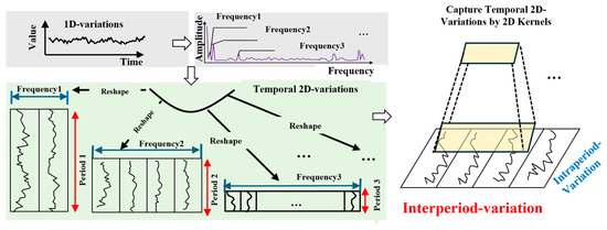
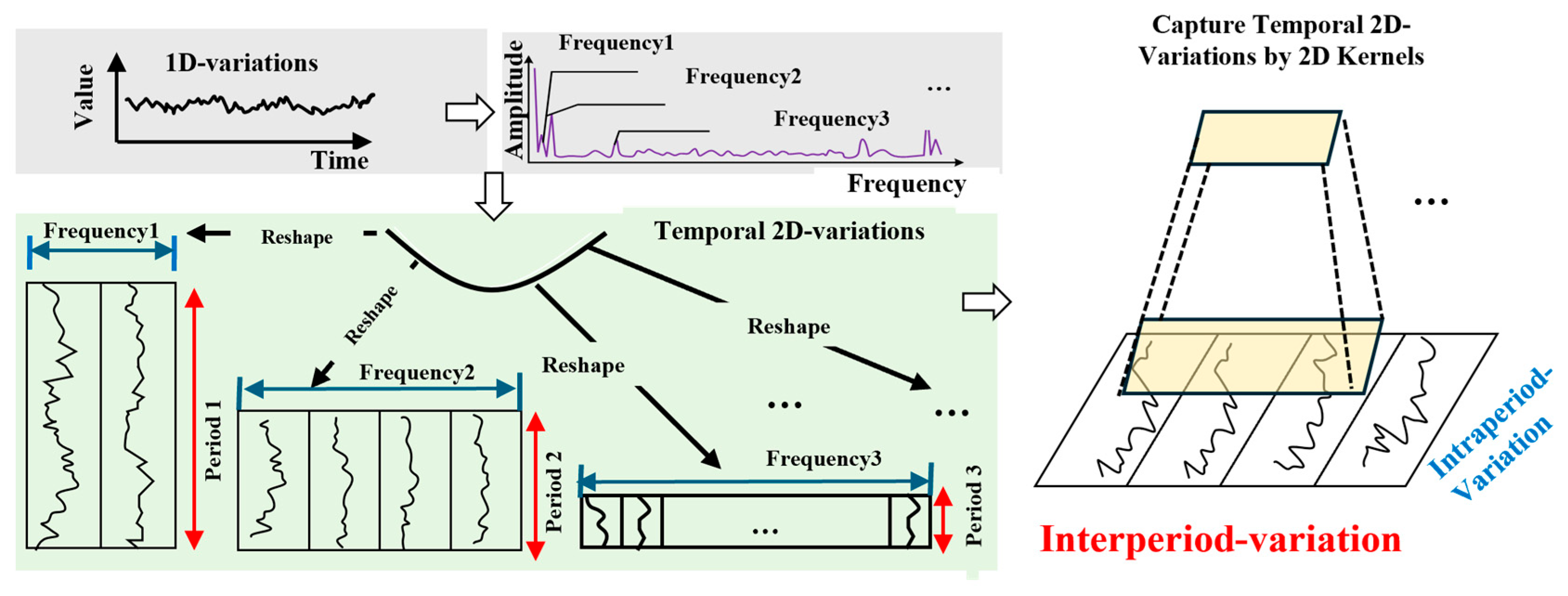
Traditional methods face challenges when dealing with the complex variations in time series, as they typically attempt to capture these changes directly from one-dimensional time series, overlooking the multi-periodicity inherent in the data. Wu et al. [26] proposed the TimesNet model, which reshapes 1D time series into a set of 2D tensors to capture the multi-periodicity and uses Convolutional Neural Networks (CNNs) to learn the patterns of the series. This approach enables the model to capture complex patterns within the time series and make accurate predictions for the future. where the time-series data are expanded from 1D to 2D representation, as illustrated in Figure 1.

Figure 1. Transformation of the 1D time series into a structured 2D tensor [26].

First, for a time series of length $T$ with $C$ recorded variables, the original 1D form is $X_{1D}\in {ℝ}^{T\times C}$. The time series is analyzed in the frequency domain using the Fast Fourier Transform (FFT), as shown below:

$$A=Avg\left(Amp\left(FFT\left(X_{1D}\right)\right)\right),\left\{f_1,\dots ,f_k\right\}=\underset{f_{\ast }\in \left\{1,\dots ,\left[{\displaystyle \frac{T}{2}}\right]\right\}}{\arg Topk},p_i=⌈{\displaystyle \frac{T}{f_i}}⌉,i\in \left\{1,\dots ,k\right\}$$

(1)

Here, $FFT\left(\cdot \right)$ and $Amp\left(\cdot \right)$ denote the fast Fourier transform and the computation of amplitude, respectively. $A$ represents the amplitude at each frequency, obtained by applying $Avg\left(\cdot \right)$ across the $C$ dimensional channel axis.

To capture the most representative signal features, only the $k$ components with the highest amplitudes are filtered to identify the key frequency sequence $\left\{f_1,\dots ,f_k\right\}$. In this context, $k$ functions as a tunable hyperparameter that governs the density of frequency extraction. Subsequently, these selected frequencies are mapped to their respective $k$ periodic lengths $\left\{p_1,\dots ,p_k\right\}$. Equation (1) is summarized as follows:

$$A,\left\{f_1,\dots ,f_k\right\},\left\{p_1,\dots ,p_k\right\}=Period\left(X_{1D}\right)$$

(2)

Finally, by using the identified frequency set $\left\{f_1,\dots ,f_k\right\}$ and their associated period lengths $\left\{p_1,\dots ,p_k\right\}$, the initial 1D temporal data $X_{1D}\in {ℝ}^{T\times C}$ is remapped into a multi-dimensional collection of 2D tensors as:

$$X_{2D}^i=\mathrm{Re}shap{e}_{p_i,f_i}\left(Padding\left(X_{1D}\right)\right),i\in \left\{1,\dots ,k\right\}$$

(3)

Here, $Padding\left(\cdot \right)$ denotes zero-padding along the temporal dimension to ensure compatibility with $\mathrm{Re}shap{e}_{p_i,f_i}\left(\cdot \right)$. Specifically, the Padding operation extends the original 1D time-series by appending zeros (or replicating boundary values) to ensure that its total length is an exact multiple of the detected period length. Subsequently, the Reshape operation folds this padded 1D sequence into a 2D tensor format. This topological transformation explicitly aligns the intra-period variations (short-term local dynamics) and inter-period variations (long-term periodic patterns) along the two distinct dimensions of the 2D tensor. The symbols $p_i$ and $f_i$ denote, respectively, the number of rows and columns of the reshaped 2D tensor.

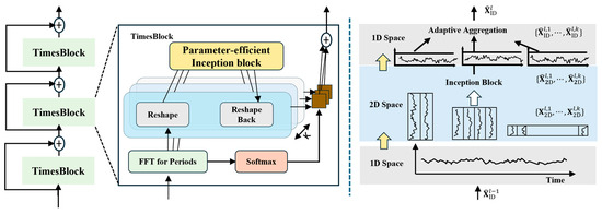
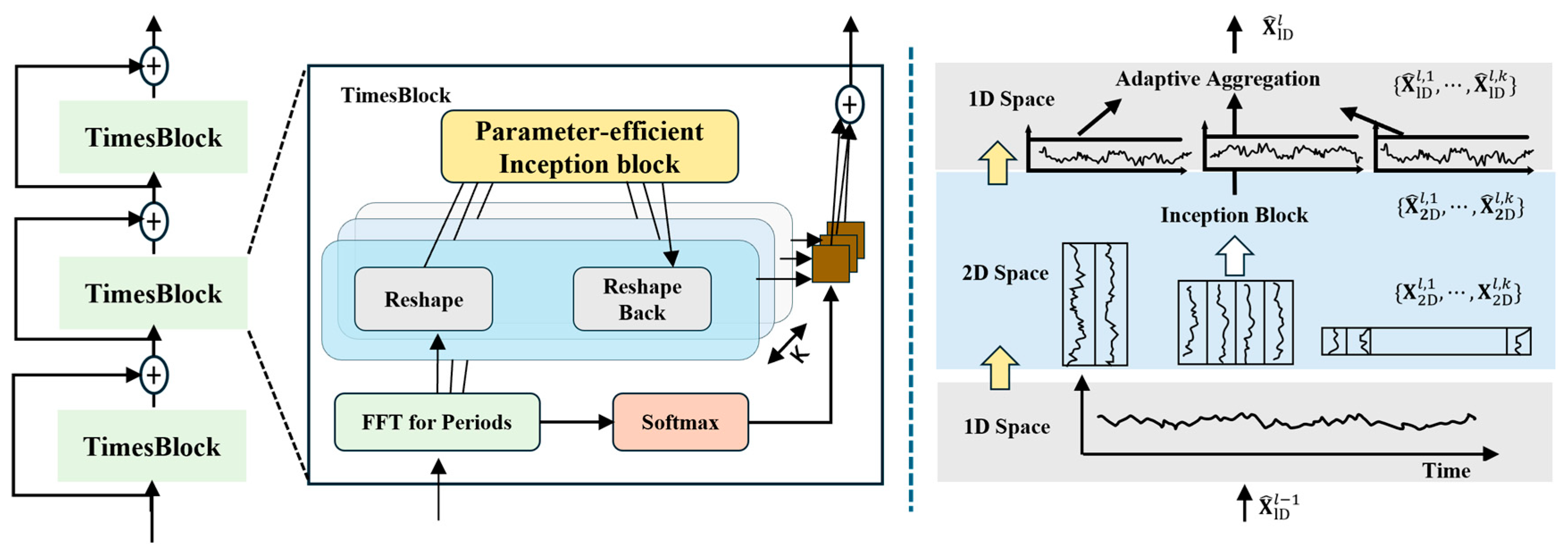
TimesNet is composed of a stack of TimesBlocks, with the TimesBlock serving as its core module. The overall architecture of TimesNet is shown in Figure 2. Given a 1D input time series $X_{1D}\in {ℝ}^{T\times C}$ of length $T$ the raw input is first mapped by an embedding layer to a deep feature representation $X_{1D}^0\in {ℝ}^{T\times d_{\mathrm{mod}el}}$ by the embedding layer. For the l-th layer of TimesNet, the input is $X_{1D}^{l-1}\in {ℝ}^{T\times d_{\mathrm{mod}el}}$, and this process can be formalized as:

$$X_{1D}^l=TimesBlock\left(X_{1D}^{l-1}\right)+X_{1D}^{l-1}$$

(4)

Figure 2. Overall architecture of TimesNet [26].

Specifically, each TimesBlock comprises the following sub-processes:

(1)

Folding the time series (1D to 2D). Extract the periodicities from the 1D input time-series features and transform them into a 2D temporal representation. The calculation formula is as follows:

$$A^{l-1},\left\{f_1,\dots ,f_k\right\},\left\{p_1,\dots ,p_k\right\}=Period\left(X_{1D}^{l-1}\right),$$

(5)

$$X_{2D}^{l,i}=\mathrm{Re}shap{e}_{p_i,f_i}\left(Padding\left(X_{1D}^{l-1}\right)\right),i\in \left\{1,\dots ,k\right\}$$

(6)

(2)

Extract a 2D representation of temporal variations. After completing the 2D transformation, the two-dimensional tensor is processed by a parameter-efficient Inception module [36]. The calculation formula is as follows:

$${\widehat{X}}_{2D}^{l,i}=Inception\left(X_{2D}^{l,i}\right),i\in \left\{1,\dots ,k\right\}$$

(7)

(3)

Unfolding the time series (2D to 1D). Convert the learned 2D representation ${\widehat{X}}_{2D}^{l,i}$ back to the 1D space ${\widehat{X}}_{1D}^{l,i}$ for feature aggregation. A $Trunc\left(\cdot \right)$ operation is applied to truncate the padded portion, restoring the sequence length from $\left(p_i\times f_i\right)$ to the original $T$, as follows:

$${\widehat{X}}_{1D}^{l,i}=Trunc\left(\mathrm{Re}shap{e}_{1,\left(p_i\times f_i\right)}\left({\widehat{X}}_{2D}^{l,i}\right)\right),i\in \left\{1,\dots ,k\right\}$$

(8)

(4)

Adaptive aggregation. Finally, the $k$ distinct 1D representations $\{{\widehat{X}}_{1D}^{l,i},\dots ,{\widehat{X}}_{1D}^{l,k}\}$ are fused for use by the next layer. The amplitude matrix $A$ reflects the relative importance of the selected frequencies and periods, indicating the salience of each transformed 2D tensor. Guided by these amplitudes, the 1D representations are aggregated via weighted fusion, as follows:

$${\widehat{A}}_{f_1}^{l-1},\dots ,{\widehat{A}}_{f_k}^{l-1}=Soft\max \left(A_{f_1}^{l-1},\dots ,A_{f_k}^{l-1}\right)$$

(9)

$$X_{1D}^l={\displaystyle \sum _{i=1}^k{\widehat{A}}_{f_i}^{l-1}}\times {\widehat{X}}_{1D}^{l,i}$$

(10)

2.3. NLinear

Transformers now dominate sequence modeling, and many variants have been developed specifically for time-series forecasting, especially for long-term prediction (LTSF). However, despite positional encodings and sub-sequence embeddings, the permutation-invariant nature of self-attention can dilute temporal order-central to time-series modeling. To address this, Zeng et al. [28] introduced LTSF–Linear and systematically compared it with multiple Transformer variants on nine real-world datasets, showing that simple linear models consistently outperform Transformer-based approaches.

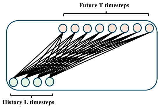
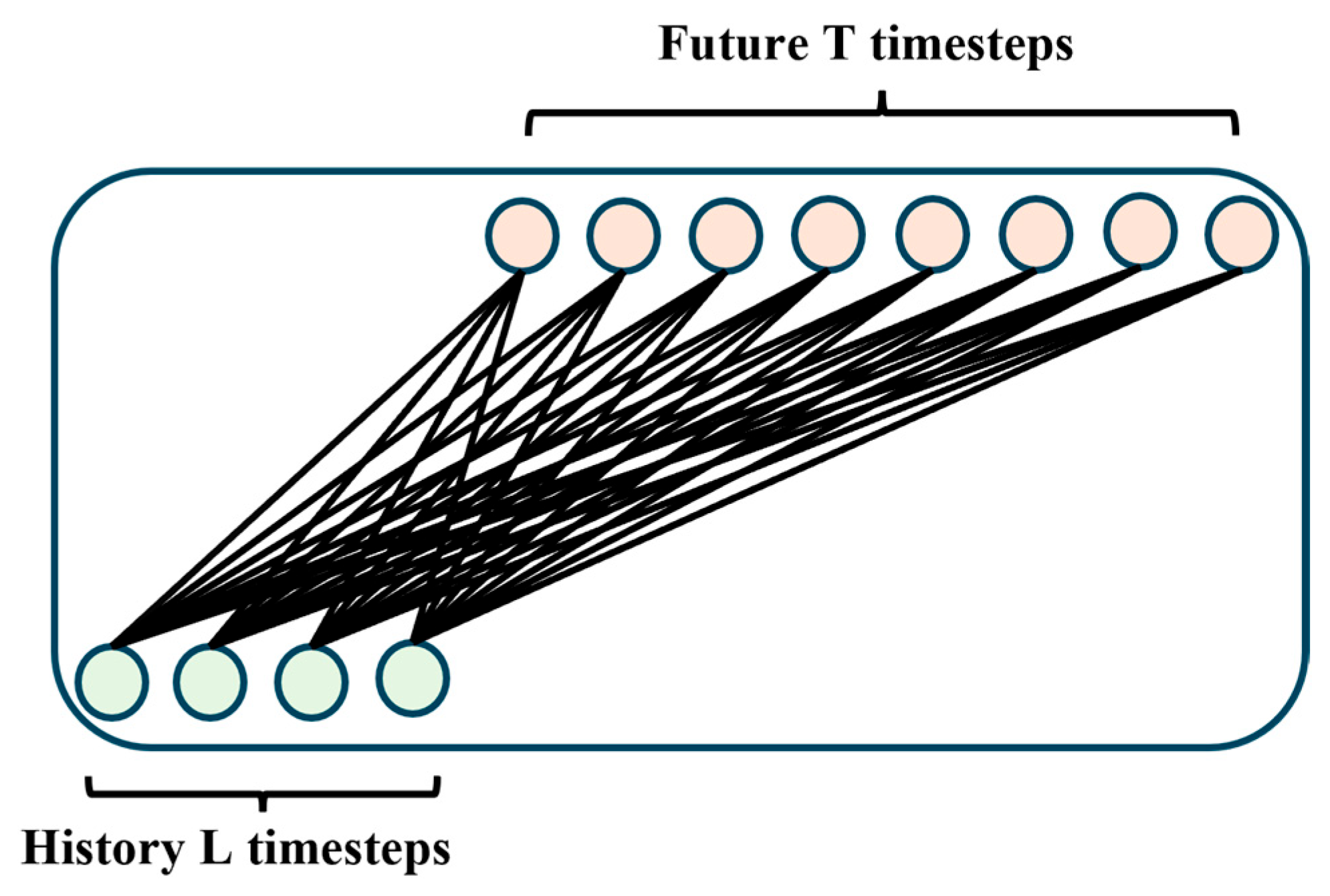
LTSF–Linear adopts a single-layer linear architecture to perform regression on historical sequences, enabling the direct generation of future predictions. Its structure is depicted in Figure 3. The LTSF–Linear family comprises Linear, DLinear, and NLinear. Linear forecasts future values by directly regressing the historical series via a weighted summation; the computation is as follows:

$${\tilde{X}}_i=W{X}_i,W\in {ℝ}^{T\times L}$$

(11)

where ${\tilde{X}}_i$ and $X_i$ denote, respectively, the prediction and the input of the i-th variable.

Figure 3. Architecture of the LTSF-Linear.

NLinear is a normalization-based variant of Linear. It first subtracts the last observed value from the input before feeding it into the linear layer, and then adds this value back to the output, thereby mitigating distribution drift and improving forecasting accuracy. The computation is as follows:

$$X_n=X_i-x_l$$

(12)

$${\tilde{X}}_i=W{X}_n+x_l$$

(13)

where $X_n$ denotes the normalized input, and $x_l$ denotes the last value of the input sequence.

2.4. STL–TimesNet–NLinear Model

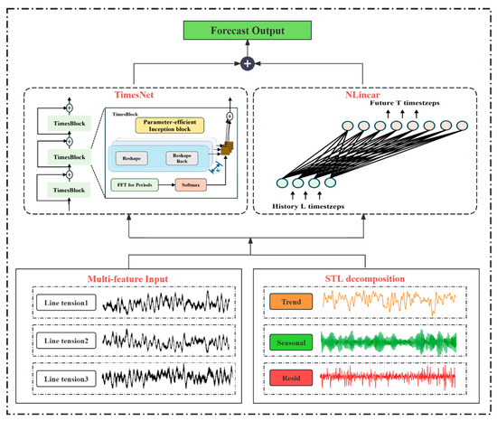
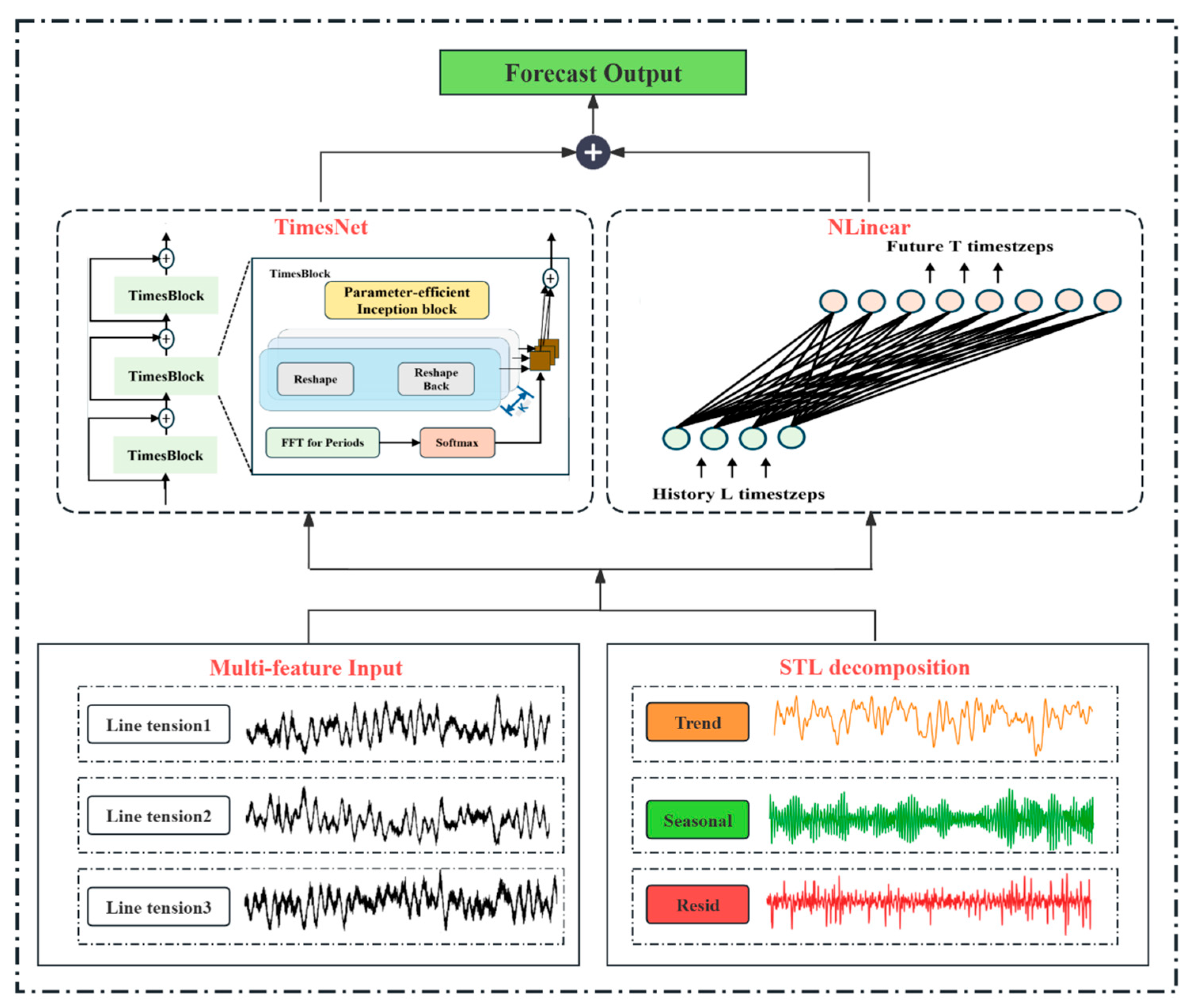
A novel predictive framework integrating STL, TimesNet, and NLinear is developed in this research to tackle the challenges of short-term FOWT response forecasting. The core mechanism relies on utilizing the STL algorithm to decouple the raw observational sequence into distinct seasonal, trend, and residual sub-signals, which are subsequently merged with relevant feature sets to construct a refined input space. By using TimesNet’s capability to map complex 2D temporal variations, the model can decode both intra- and inter-period cyclical patterns. Concurrently, the NLinear algorithm handles the macroscopic trending behaviors. The framework synthesizes these parallel analytical streams to generate highly accurate final predictions, as visually detailed in Figure 4.

Figure 4. Architecture of the STL–TimesNet–NLinear.

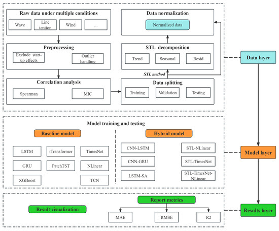
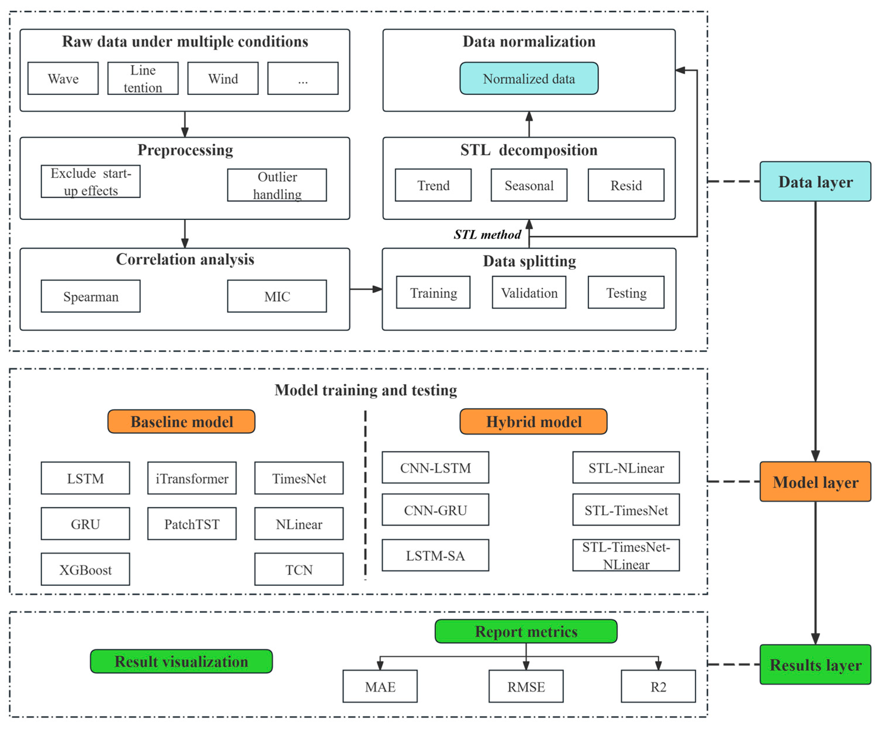
To clearly articulate the research scheme, Figure 5 presents the overall workflow, which is organized into three layers: the data layer, the model layer, and the results layer. In the data layer, we first preprocess the raw data, conduct feature selection using correlation analysis tools, perform a training–validation–test split, and standardize the data, noting that for STL the series is decomposed prior to standardization. In the model layer, we train and test a total of 14 models, encompassing both baseline and hybrid architectures. Finally, in the results layer, we visualize the forecasting outputs and report multiple evaluation metrics derived from the trained models.

Figure 5. Overview of the workflow.

3. Case Study

3.1. Numerical Simulation of the 5 MW FOWT

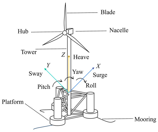
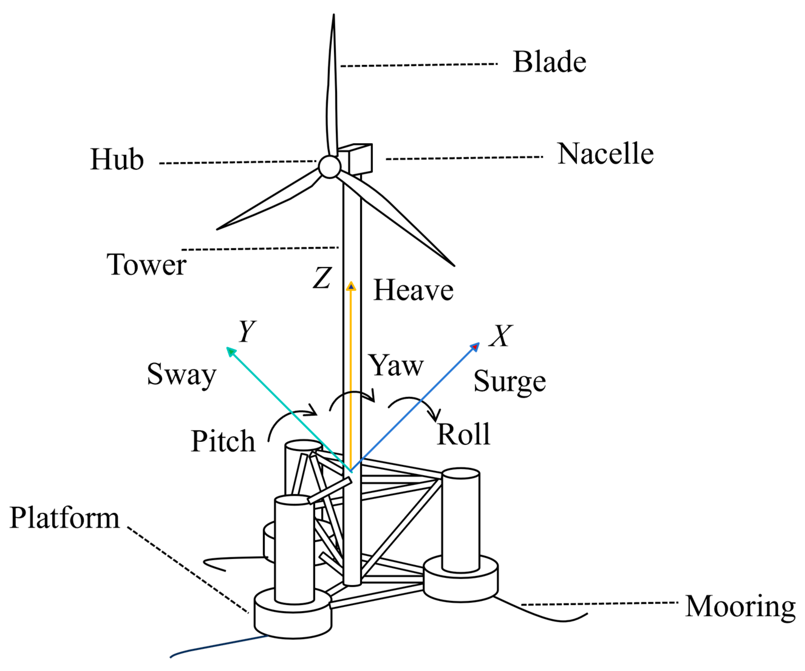
The FOWT model used in this study is the OC4 DeepCwind semi-submersible FOWT. The hub height of the turbine is 90 m, and the rotor has a diameter of 126 m. The semi-submersible floating platform features horizontal and diagonal cross-bracings, a central support column for the tower, and three offset columns with larger diameters. To mitigate excessive heave motions, heave plates are attached to the bottoms of the base columns. The platform is anchored using three catenary mooring lines spaced 120 degrees apart, which provide restoring forces and moments for the surge, sway, and yaw DOFs. Table 1 summarizes the key properties of the DeepCwind semi-submersible FOWT, including hub height, cut-in, rated, and cut-out wind speeds, center of mass (CM), moments of inertia, and the mass of major components [37]. The simulation data used in this article are based on the verification and validation (V&V) activities performed in IEA Wind Task 30, specifically the Offshore Code Comparison Collaboration (OC4–OC6) projects [37,38,39]. This is because the aero-hydro-servo-elastic modeling capabilities of open-source wind turbine simulation tool (OpenFAST) have been rigorously validated against wave tank tests and full-scale prototype measurements. This ensures that the motion data used for training inherently will contain validated nonlinear dynamic coupling present in the FWT system, allowing the accuracy improvements observed in this study to hold genuine practical significance for real-world offshore engineering operations. A schematic of the FOWT structure and its 6-DOFs is illustrated in Figure 6.

Table 1. Summary properties of the DeepCwind semi-submersible FOWT.

Item	Value
Rotor orientation	Upwind, 3 blades
Cut-in/Rated/Cut-out wind speeds	3 m/s, 11.4 m/s, 25 m/s
Rotor mass	110,000 kg
Nacelle mass	240,000 kg
Tower mass	347,460 kg
Hub height	90 m
CM (x, y, z) of the platform	(0, 0, −13.46)
Platform draft	20 m
Platform roll inertia about CM	6.827 × 109 kg·m2
Platform pitch inertia about CM	6.827 × 109 kg·m2
Platform yaw inertia about CM	1.226 × 1010 kg·m2

Figure 6. Schematic illustration of the semi-submersible FOWT structure and definitions of the 6-DOFs motions.

The OpenFAST v4.1.2, developed by the National Renewable Energy Laboratory (NREL), is utilized in this study to simulate the aero-hydro-servo-elastic responses of the target FOWT under specific environmental conditions. Previous research has validated the modeling capability of OpenFAST, confirming its accuracy and reliability [38,40]. The preprocessing tool TurbSim is employed to generate a synthetic three-dimensional turbulent wind field using the Kaimal exponential and spectral coherence model. To capture the coupled dynamics of the FOWT, rotor aerodynamic responses are simulated via the AeroDyn code utilizing the Blade Element Momentum (BEM) method. Simultaneously, the HydroDyn package calculates the platform’s hydrodynamic load-effects by combining potential flow formulations with Morison’s equation for viscous drag estimation. The mooring lines are represented using a spatial lumped-mass discretization approach. Furthermore, a variable-speed generator torque and a collective blade-pitch control are used.

Three representative environmental load cases are used, corresponding to the cut-in, rated, and cut-out operating regions. According to the DNV-ST-0437 [41], the vertical wind profile is to be approximated using a power–law model featuring a shear exponent of 0.12. Stochastic irregular waves are modelled using the JONSWAP spectrum, with a peakedness parameter of 3.3. The total computational duration for each load case is set to 4000 s; however, the initial 500 s transient period is discarded to eliminate the non-stationary parts. The detailed environmental parameters, including turbulence intensity (TI), significant wave height (Hs), and peak spectral period (Tp), are summarized in Table 2.

Table 2. Parameters of three Environmental conditions.

Item	${\mathit{u}}_{\mathit{h}\mathit{u}\mathit{b}}$	TI	${\mathit{H}}_{\mathit{s}}$	${\mathit{T}}_{\mathit{p}}$
EC1	8 m/s	17.4%	2.3 m	8.3 s
EC2	11 m/s	15.1%	2.8 m	8.7 s
EC3	15 m/s	13.5%	3.4 m	9.8 s

3.2. Data Processing

The raw 6-DOFs motion response data of the support platform obtained from OpenFAST has a sampling frequency of 40 Hz. The sampling frequency is reduced to 10 Hz to retain the signal characteristics while reducing data size. Each simulation under the selected environmental conditions (ECs) lasts for 4000 s. To exclude the start-up effects, only the simulation data from 500 to 4000 s are retained, resulting in 35,000 data points collected for each EC.

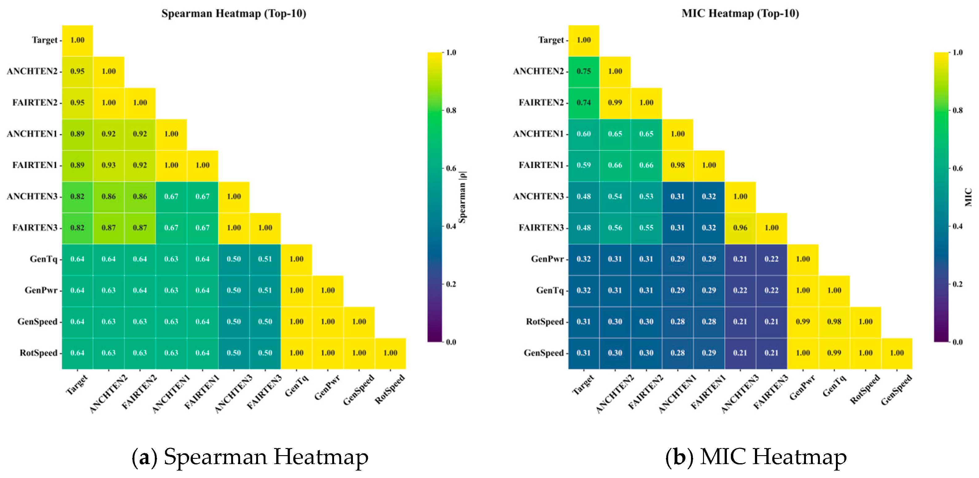
Studies have shown that using wave elevation and mooring force as multi-feature inputs can improve prediction accuracy [42]. To curb the sharp rise in training cost caused by high-dimensional inputs, we perform feature screening by combining Spearman rank-correlation analysis with the Maximal Information Coefficient (MIC). Figure 7 reports the top-10 features under Spearman and MIC, respectively; we take the intersection of these two sets and, considering data availability in practical deployments, ultimately select fairlead tension as the multi-feature input.

Figure 7. Heatmap of spearman and MIC analysis results.

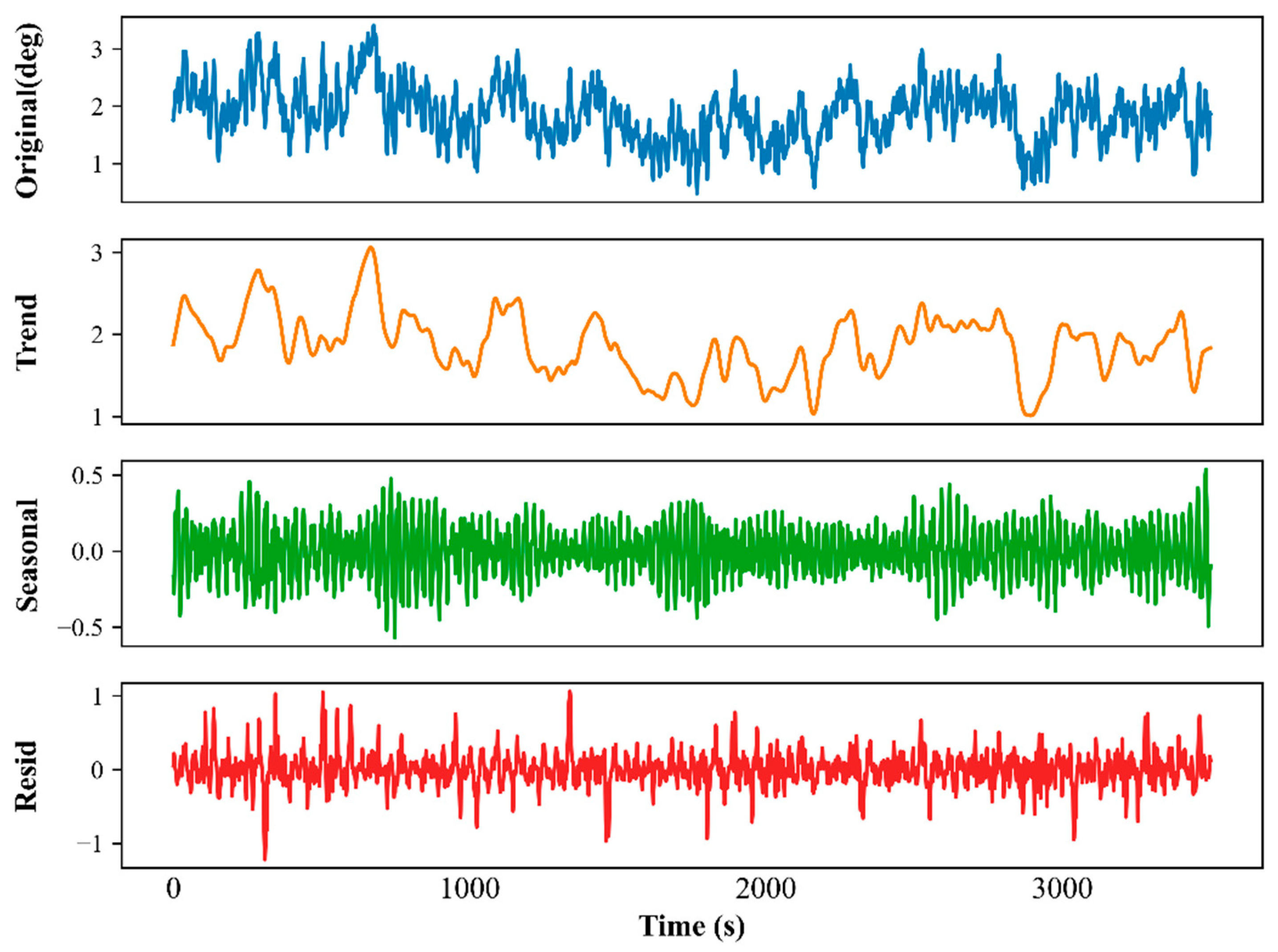
Following the feature screening process, the data matrix is split into 60% training, 20% validation, and 20% testing sets. For architectures incorporating the STL mechanism, the target sequence is first decomposed into its constituent components. Using the pitch response under EC1 as a representative case, Figure 8 shows the extracted macroscopic trend, periodic seasonality, and random residual components. As illustrated, the top panel (Original) displays the raw pitch motion, where multi-periodic wave-frequency oscillations are superimposed upon an irregular low-frequency drift. The second panel isolates the trend component ($T_t$), which physically aligns with the low-frequency slow-drift dynamics induced by second-order wave forces and wind turbulence. This non-stationary trend is specifically targeted by the NLinear module within our framework to reduce the effects of distribution shifts. The third panel extracts the seasonal component ($S_t$), corresponding to the wave-frequency responses driven by first-order wave excitation. The TimesNet module is assigned to this component to use, its capability to capture intricate intra-period and inter-period variations. Lastly, the bottom panel represents the residual component ($R_t$), encompassing stochastic noise and unpredictable high-frequency fluctuations. Following dataset standardization and the aforementioned STL decomposition, the continuous time-series data—comprising the target 6-DOF motions and the selected multi-feature inputs (i.e., fairlead tensions)—are transformed into input–output tensor pairs via a sliding window mechanism. To ensure a fair comparison, all models evaluated in this study utilize a look-back window of length $L=\left\{200,400\right\}$ steps (corresponding to 20 and 40 s of historical dynamics at a 10 Hz sampling rate) to forecast a future horizon of $T=\left\{50,100\right\}$ steps (representing 5 and 10 s of future 6-DOF motion responses, respectively). The sliding window advances along the time axis with a stride of 1, generating a set of overlapping sequences to construct the three-dimensional tensors required for training the deep learning architectures.

Figure 8. STL decomposition of pitch motion under EC1.

To accelerate the convergence rate during the training phase, the raw dataset initially undergoes a standard scaling process. Upon completion of the model training, an inverse scaling procedure is applied to both the forecasted outputs and the ground truth. This crucial step ensures that the FOWT platform’s 6-DOF dynamic responses are accurately restored to their original physical dimensions. The mathematical expressions governing these bidirectional transformations are detailed below:

$$x_{trans}={\displaystyle \frac{x-\mu }{\sigma }}$$

(14)

$$\mu ={\displaystyle \frac{1}{n}}{\displaystyle \sum _{i=1}^n{x}_i}$$

(15)

$$\sigma =\sqrt{{\displaystyle \frac{1}{n-1}}{\displaystyle \sum _{i=1}^n{(x_i-\mu )}^2}}$$

(16)

$$x=x_{trans}\sigma +\mu$$

(17)

Here, $x_{trans}$ represents the normalized data, $x$ represents the original data, $\mu$ represents the mean value, and $\sigma$ represents the standard deviation.

3.3. Training and Testing Models

The modelling stage for training and evaluation is performed after the data processing. As demonstrated by Guo et al. [13,43], short-term forecasting of FOWT motions generally involves high-fidelity predictions over a prediction horizon on the order of tens of seconds. Accordingly, this study considers two PATs of 5 s and 10 s. To evaluate the advantages of the proposed method, we trained 14 models at this stage. As summarized in Table 3, these include both baseline and hybrid configurations, covering machine learning (e.g., XGBoost), CNN-based architectures (e.g., Temporal Convolutional Network (TCN)), classical RNNs and their hybrid models, as well as the latest state-of-the-art time-series architectures.

Table 3. Overview of the models used in this study.

Baseline Models	Hybrid Models
LSTM	CNN-LSTM CNN-GRU LSTM–SelfAttention (SA) STL–TimesNet STL–NLinear STL–TimesNet–NLinear
GRU
PatchTST
iTransformer
TimesNet
NLinear
XGBoost
TCN

The maximum number of training epochs is set to 50. To improve training efficiency, we adopt an early stopping strategy: the validation loss is continuously monitored, and the model is checkpointed when the minimum validation loss is observed; if the validation loss fails to decrease within a predefined patience window, training is terminated to reduce unnecessary computation and mitigate overfitting. In this study, the early-stopping patience is set to 10, meaning that training stops early if the validation loss shows no improvement for 10 consecutive epochs. To ensure experimental reproducibility and maintain a fair comparative environment, all baseline models evaluated in this study were implemented utilizing the widely recognized open-source time-series forecasting frameworks, Darts [44] and TFB [34] (Time Series Forecasting Benchmark). We deliberately refrained from exhaustive, model-specific manual hyperparameter tuning, as such practices inherently risk introducing human bias or forcing the models to overfit the test set. Instead, all network architectures and optimization pipelines uniformly adopted the standardized, default hyperparameter configurations recommended by both libraries for multivariate forecasting tasks.

Open-source libraries are utilized in this study for model construction and training. For data processing, libraries such as NumPy, Pandas, and Scikit-learn are employed. The Python version used is 3.8.10, with PyTorch 1.7.1 for model construction and CUDA 11.0 to accelerate GPU computations. For visualization, the Matplotlib v3.7.5 library in Python and the ggplot library in the R language (version 4.4.2) are used to create visual plots. The experiments are conducted on an Ubuntu 20.04.3 LTS system, using an NVIDIA A10 GPU with 24 GB memory for model training and testing.

3.4. Evaluation of Metrics

The forecasting performance of the proposed model is quantitatively evaluated using three statistical indicators: MAE, root mean squared error (RMSE), and R². The respective mathematical definitions are presented as follows:

$$\mathrm{MAE}={\displaystyle \frac{1}{n}}{\displaystyle \sum _{j=1}^n|y_j-{\widehat{y}}_j|}$$

(18)

$$\mathrm{RMSE}=\sqrt{{\displaystyle \frac{1}{n}}{\displaystyle \sum _{j=1}^n{(y_j-{\widehat{y}}_j)}^2}}$$

(19)

$${\mathrm{R}}^2=1-{\displaystyle \frac{{\displaystyle {\sum }_{j=1}^n{(y_j-{\widehat{y}}_j)}^2}}{{\displaystyle {\sum }_{j=1}^n{(y_j-\overline{y})}^2}}}$$

(20)

In the above formulas, $y_j$ and ${\widehat{y}}_j$ respectively represent the actual value and the predicted value at time $j$. Where $\overline{y}$ represents the average value of the actual values, and $n$ is the number of data values in the test set.

4. Results and Discussion

4.1. Motion Response Result Analysis

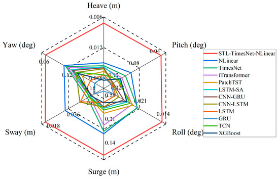
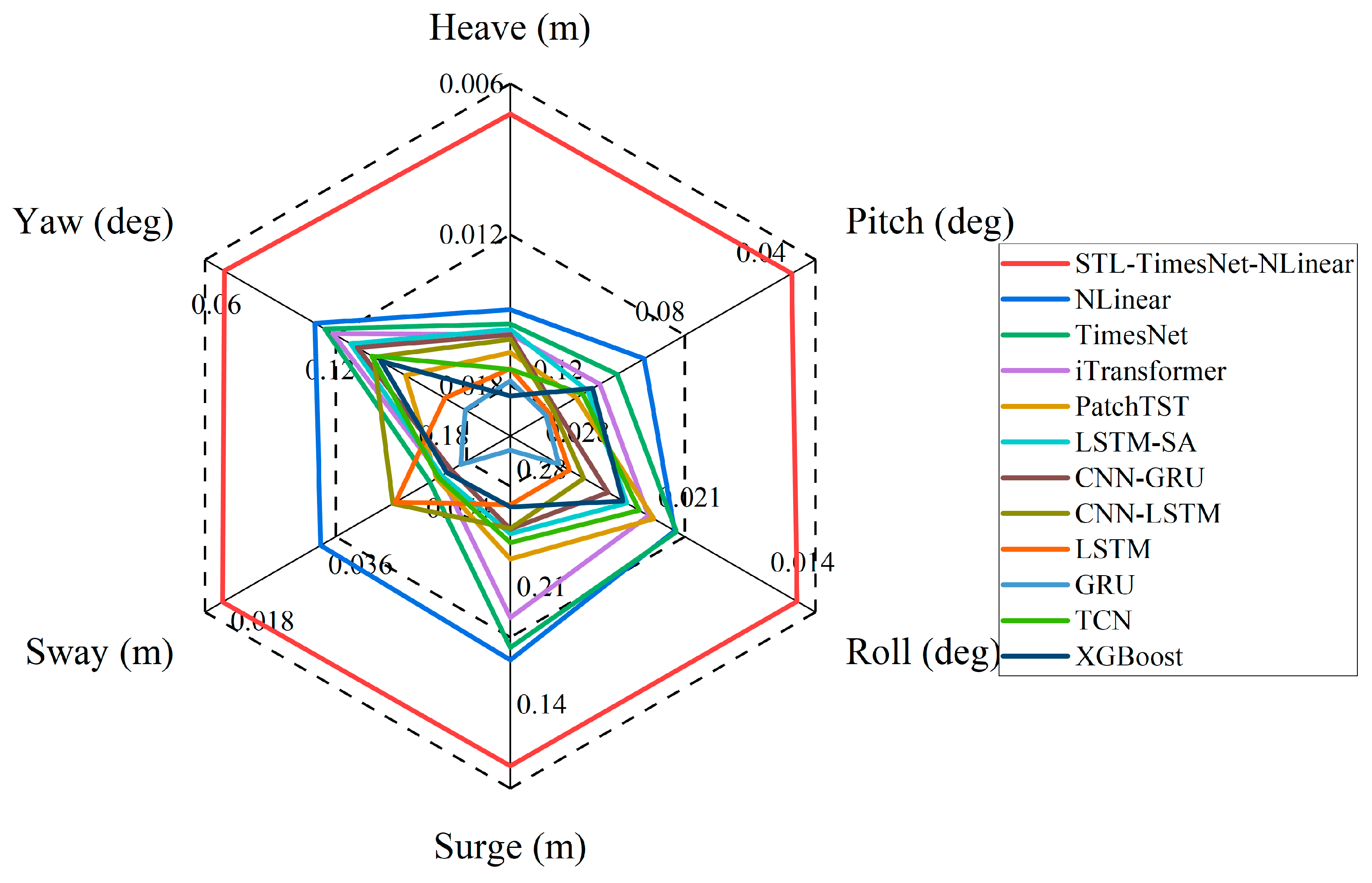
To assess the feasibility and superiority of the proposed STL–TimesNet–NLinear framework for predicting the 6-DOFs motion responses of the FOWT support platform, we performed comparative experiments under EC1 with a PAT of 5 s. The benchmark set includes state-of-the-art time-series models such as iTransformer, PatchTST, TimesNet, and NLinear; traditional RNNs like LSTM and GRU; and common RNN-based hybrid models. In addition, we also included the machine learning method XGBoost and the CNN-based TCN model. Figure 9 presents a radar chart of MAE across the six motion components (heave, pitch, roll, surge, sway, yaw). The results indicate that the proposed STL–TimesNet–NLinear consistently attains the lowest MAE across the DOFs, demonstrating superior prediction accuracy compared with the competing methods.

Figure 9. MAE results of different methods across the 6-DOFs.

4.1.1. Comparison of the Different Methods for Motion Response Prediction

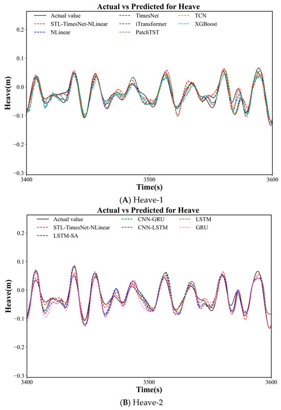
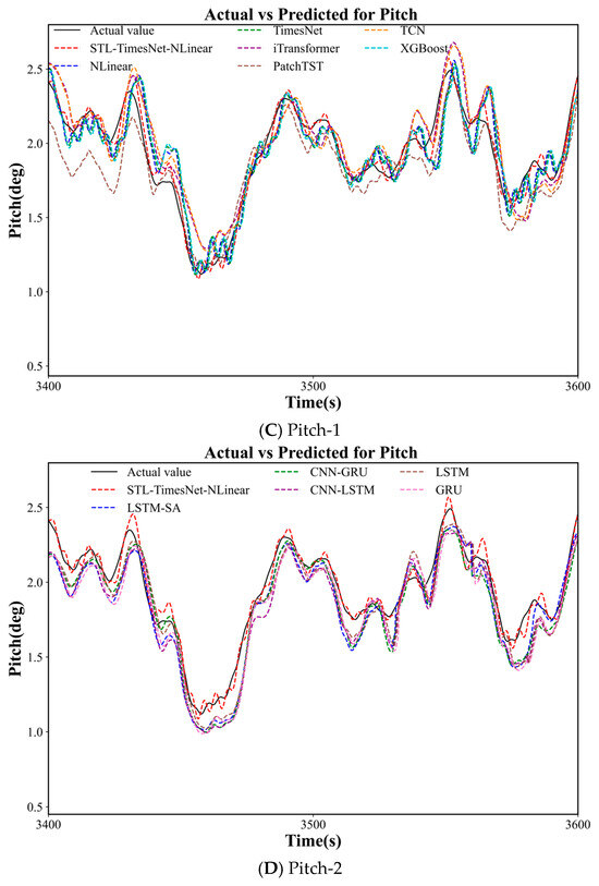
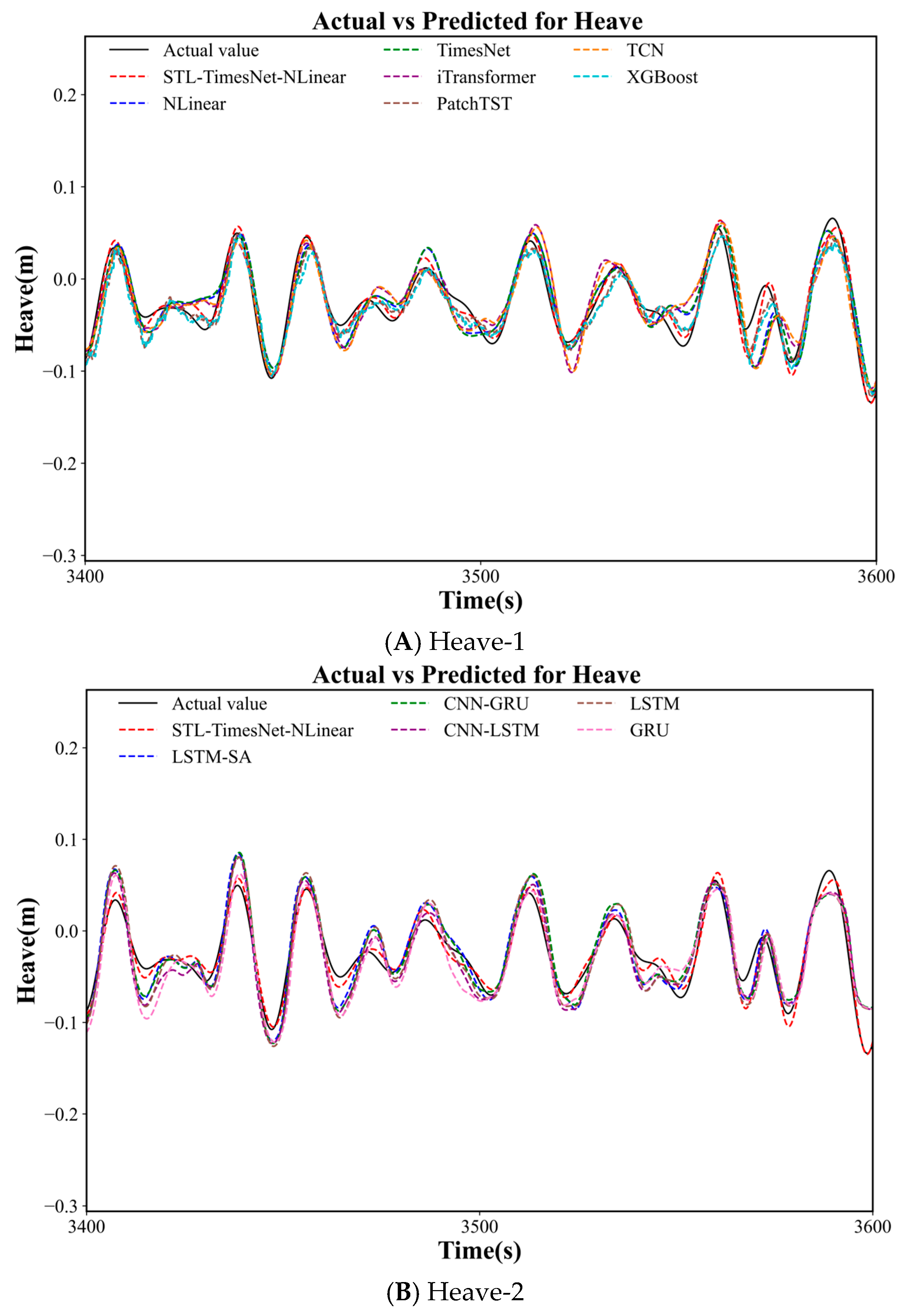
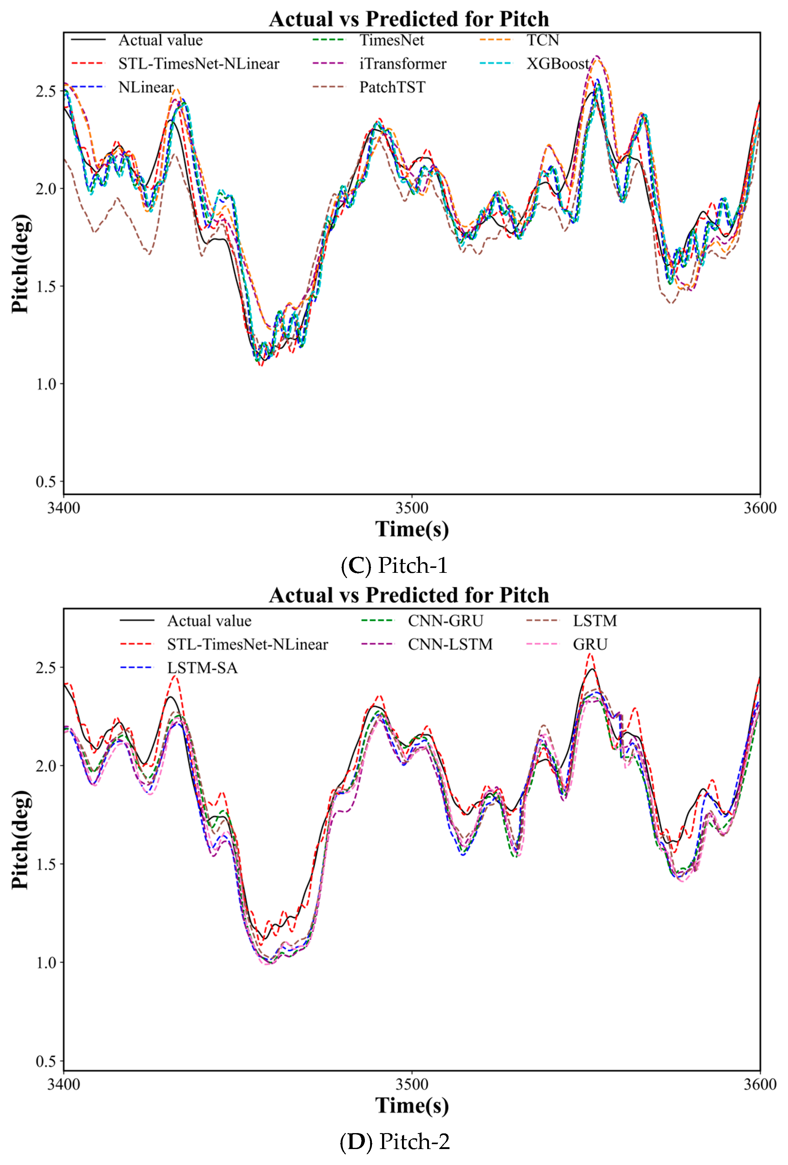
Using simulated data generated from numerical simulations, the STL–TimesNet–NLinear model and the comparative models were trained on the 6-DOFs motion response data of the FOWT support platform. The predicted outputs were then compared with the ground-truth data from the test set. Figure 10 illustrates the comparative prediction results for selected test samples of the heave and pitch motions under EC1. Two separate figures are presented for the heave and pitch responses due to the large number of benchmark models. The first figure compares the proposed method with state-of-the-art models in the time-series domain, as well as the machine learning model XGBoost and the CNN-based model TCN, while the second contrasts it with RNN-based models and their hybrid variants. In these plots, the black line denotes the ground truth, the red line represents the predictions of the STL–TimesNet–NLinear model, and the remaining colors correspond to other comparative models. As observed, the STL–TimesNet–NLinear model consistently produces predictions that are closest to the ground truth, particularly around the peaks and valleys, while also preserving the overall dynamic trend. This indicates that it achieves the highest predictive accuracy among all evaluated models.

Figure 10. Predicted heave and pitch responses from different models for selected test samples.

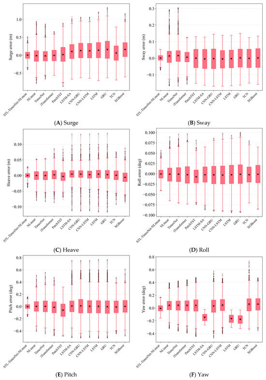
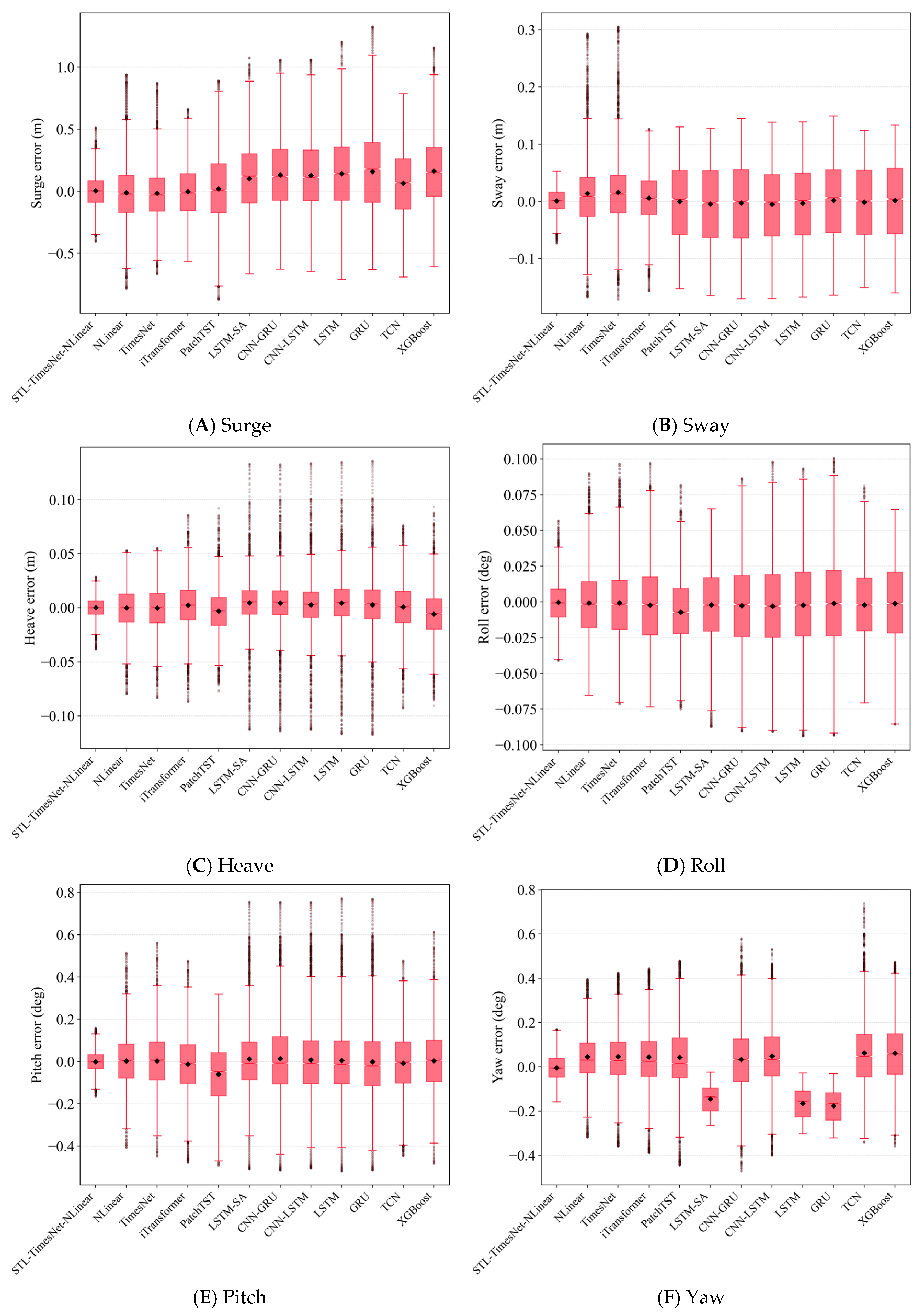
Figure 11 presents the boxplots of prediction errors for all 6-DOFs across the evaluated models. In each subplot, the black diamond denotes the mean prediction error, while the circular markers above and below the box indicate outliers. It is evident that the proposed STL–TimesNet–NLinear model exhibits highly concentrated error distributions across all DOFs: the upper and lower bounds of the box remain tightly clustered around zero, the number of outliers is minimal, and the fluctuation range is the smallest among all models. Moreover, the mean error is consistently close to zero, demonstrating the model’s strong robustness and stability.

Figure 11. Boxplots of prediction errors for different models.

In addition, advanced time-series forecasting models such as NLinear, TimesNet, iTransformer, and PatchTST achieve noticeably lower errors and reduced variability compared with RNN-based models and their hybrid variants, as well as the XGBoost and TCN models. This further verifies their inherent advantages in capturing temporal dependencies and improving predictive performance in short-term dynamic response forecasting of floating structures.

4.1.2. Comparison of Prediction Evaluation Metrics

To further evaluate the performance of different models in short-term motion response prediction of FOWTs, Table 4 and Table 5 compare the proposed STL–TimesNet–NLinear model with several benchmark approaches under a PAT of 5 s. The performance metrics adopted, including MAE, RMSE, and R², are consistent with those defined in Section 3.4. In the tables, boldface indicates the best performance, while underlined values denote the second-best results. As shown, the proposed STL–TimesNet–NLinear model consistently achieves the lowest MAE and RMSE across all six degrees of freedom, demonstrating superior numerical fitting capability and the highest prediction accuracy among all the evaluated models. Moreover, its R² values remain above 0.95 for every DOF, indicating an excellent ability to capture the intrinsic temporal patterns of the motion responses. These results further confirm the robustness and effectiveness of the STL–TimesNet–NLinear model, particularly in handling the highly coupled and nonlinear characteristics of FOWT dynamics. Compared with both state-of-the-art time-series models and RNN-based or hybrid models, STL–TimesNet–NLinear exhibits a clear and consistent performance advantage, providing more stable predictions and significantly reduced error fluctuations under short-term forecasting conditions.

Table 4. Results of prediction evaluation metrics (Set 1).

	Surge			Sway			Heave
Model	MAE	RMSE	R2	MAE	RMSE	R2	MAE	RMSE	R2
XGBoost	0.2576	0.3273	0.9454	0.0584	0.0657	0.9806	0.0184	0.0240	0.8874
TCN	0.2365	0.2880	0.9577	0.0568	0.0639	0.9817	0.0174	0.0222	0.9036
GRU	0.2915	0.3569	0.9351	0.0574	0.0656	0.9807	0.0178	0.0250	0.8784
LSTM	0.2589	0.3198	0.9479	0.0565	0.0650	0.9810	0.0173	0.0244	0.8844
CNN-LSTM	0.2445	0.3074	0.9519	0.0553	0.0640	0.9816	0.0162	0.0231	0.8957
CNN-GRU	0.2448	0.3091	0.9513	0.0609	0.0691	0.9785	0.0160	0.0230	0.8968
LSTM-SA	0.2418	0.2938	0.9560	0.0592	0.0667	0.9800	0.0158	0.0226	0.9001
PatchTST	0.2266	0.2817	0.9596	0.0573	0.0649	0.9811	0.0160	0.0208	0.9160
iTransformer	0.1738	0.2160	0.9762	0.0352	0.0445	0.9911	0.0167	0.0215	0.9098
TimesNet	0.1665	0.2152	0.9764	0.0485	0.0675	0.9795	0.0156	0.0197	0.9244
NLinear	0.1917	0.2476	0.9688	0.0489	0.0683	0.9790	0.0150	0.0190	0.9296
STL–TimesNet–NLinear	0.1033	0.1310	0.9913	0.0172	0.0217	0.9979	0.0072	0.0091	0.9837

Table 5. Results of prediction evaluation metrics (Set 2).

	Roll			Pitch			Yaw
Model	MAE	RMSE	R2	MAE	RMSE	R2	MAE	RMSE	R2
XGBoost	0.0230	0.0276	0.8949	0.1176	0.1502	0.8836	0.1316	0.1754	0.9460
TCN	0.0220	0.0273	0.8971	0.1215	0.1551	0.8759	0.1269	0.1634	0.9531
GRU	0.0270	0.0338	0.8425	0.1359	0.1796	0.8335	0.1763	0.1896	0.9369
LSTM	0.0263	0.0327	0.8523	0.1329	0.1759	0.8404	0.1654	0.1780	0.9444
CNN-LSTM	0.0254	0.0317	0.8616	0.1320	0.1748	0.8424	0.1193	0.1593	0.9555
CNN-GRU	0.0239	0.0298	0.8773	0.1346	0.1766	0.8390	0.1280	0.1669	0.9511
LSTM-SA	0.0214	0.0265	0.9032	0.1195	0.1639	0.8614	0.1447	0.1559	0.9573
PatchTST	0.0198	0.0250	0.9138	0.1240	0.1578	0.8715	0.1158	0.1591	0.9556
iTransformer	0.0227	0.0285	0.8879	0.1148	0.1474	0.8878	0.1064	0.1455	0.9628
TimesNet	0.0211	0.0268	0.9008	0.1079	0.1378	0.9021	0.1021	0.1394	0.9659
NLinear	0.0197	0.0251	0.9132	0.0974	0.1245	0.9200	0.0970	0.1311	0.9699
STL–TimesNet–NLinear	0.0121	0.0155	0.9671	0.0394	0.0495	0.9873	0.0491	0.0599	0.9937

Specifically, the proposed model exhibits pronounced performance advantages in the heave, pitch, and roll degrees of freedom. Compared with other models that achieved the second-best results (indicated by underlines in Table 4 and Table 5), the STL–TimesNet–NLinear model achieves reductions in MAE of 52.0%, 59.5%, and 38.6%, respectively, while the RMSE decreases by 52.1%, 60.2%, and 38.0% for the same DOFs. In addition, the R² values increase by 5.8%, 7.3%, and 5.8%, demonstrating substantial improvements in capturing the underlying dynamic patterns. For the motions of surge, sway, and yaw, the proposed model achieves R² values above 0.99, with the lowest MAE and RMSE among all compared models, highlighting its exceptional accuracy and robustness across all 6-DOFs.

Among the competing approaches, the NLinear model consistently achieves the second-lowest MAE in the heave, roll, pitch, and yaw directions. TimesNet and iTransformer obtain the second-lowest MAE and RMSE, as well as the second-highest R², in the surge and sway directions, indicating their relatively strong predictive capabilities. These results confirm that state-of-the-art time-series models outperform RNN-based and hybrid RNN models, further demonstrating their advantages and research potential in short-term motion response prediction of FOWTs.

To evaluate the practical feasibility of the proposed framework for engineering applications, a computational complexity analysis was conducted. Table 6 presents the total training time (Fit_time) and single-step inference time (Inference_time) for all evaluated models. To ensure a fair comparison, all experiments were executed in the identical hardware and software environment detailed in Section 3.3, and the average runtime was calculated over three independent trials. As shown in Table 6, traditional RNN-based models (e.g., LSTM, GRU) and their hybrid variants exhibit significantly higher training costs, ranging from 1225.3 s to 1749.2 s. This is primarily attributed to their sequential data processing mechanisms, which inherently hinder parallel computation. In contrast, advanced time-series architectures benefit from parallel processing capabilities, resulting in notably reduced training times. The proposed STL–TimesNet–NLinear model requires 645.6 s for training. Although this duration is slightly higher than that of purely linear baseline models like NLinear (140.7 s) due to the requisite STL decomposition and TimesNet feature extraction, it still reduces the training time by more than 50% compared to a standard LSTM (1404.2 s). It should be noted that while the absolute values of training and inference time are hardware-dependent and may fluctuate across different GPU architectures, the relative efficiency gains and the order of magnitude of the computational latency remain consistent.

Table 6. Comparison of training and inference time for different forecasting models.

Model	Fit_Time (s)	Inference_Time (ms)
XGBoost	386.4	15.1
TCN	450.7	17.5
GRU	1225.3	15.7
LSTM	1404.2	24.6
CNN-LSTM	1614.4	35.6
CNN-GRU	1445.6	31.0
LSTM-SA	1749.2	42.5
PatchTST	499.6	1.2
iTransformer	188.8	0.7
TimesNet	590.7	1.8
NLinear	140.7	0.5
STL–TimesNet–NLinear	645.6	2.4

Note: All models were evaluated using an NVIDIA A10 GPU. Fit_time represents the total time to complete the training process, and Inference_time denotes the latency for a single-step prediction. Absolute runtimes may vary depending on specific hardware configurations.

More importantly, for short-term motion response prediction with a PAT of 5 s or 10 s, the online inference time is the critical metric for determining real-time control applicability. The results explicitly demonstrate that the proposed model achieves an ultra-fast inference time of merely 2.4 ms. An execution delay of 2.4 ms is orders of magnitude smaller than the 5 s prediction horizon. This confirms that despite its hybrid structural design, the proposed framework does not impose an excessive computational burden. Rather, it comfortably satisfies the stringent real-time computational constraints required for onboard dynamic positioning systems and safety early-warning controllers of FOWTs.

4.2. The Effect of Different PATs

As demonstrated in Section 4.1, the STL–TimesNet–NLinear model outperforms the other models in predicting the 6-DOF motion responses of the FOWT support platform. This section further examines the prediction performance of the model under different PATs. Two commonly used PAT values are selected to achieve a balanced trade-off between prediction horizon and prediction accuracy.

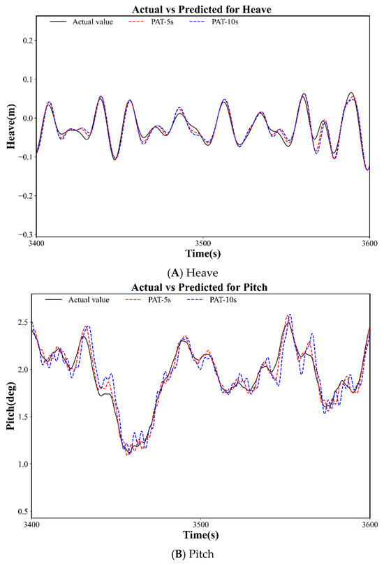
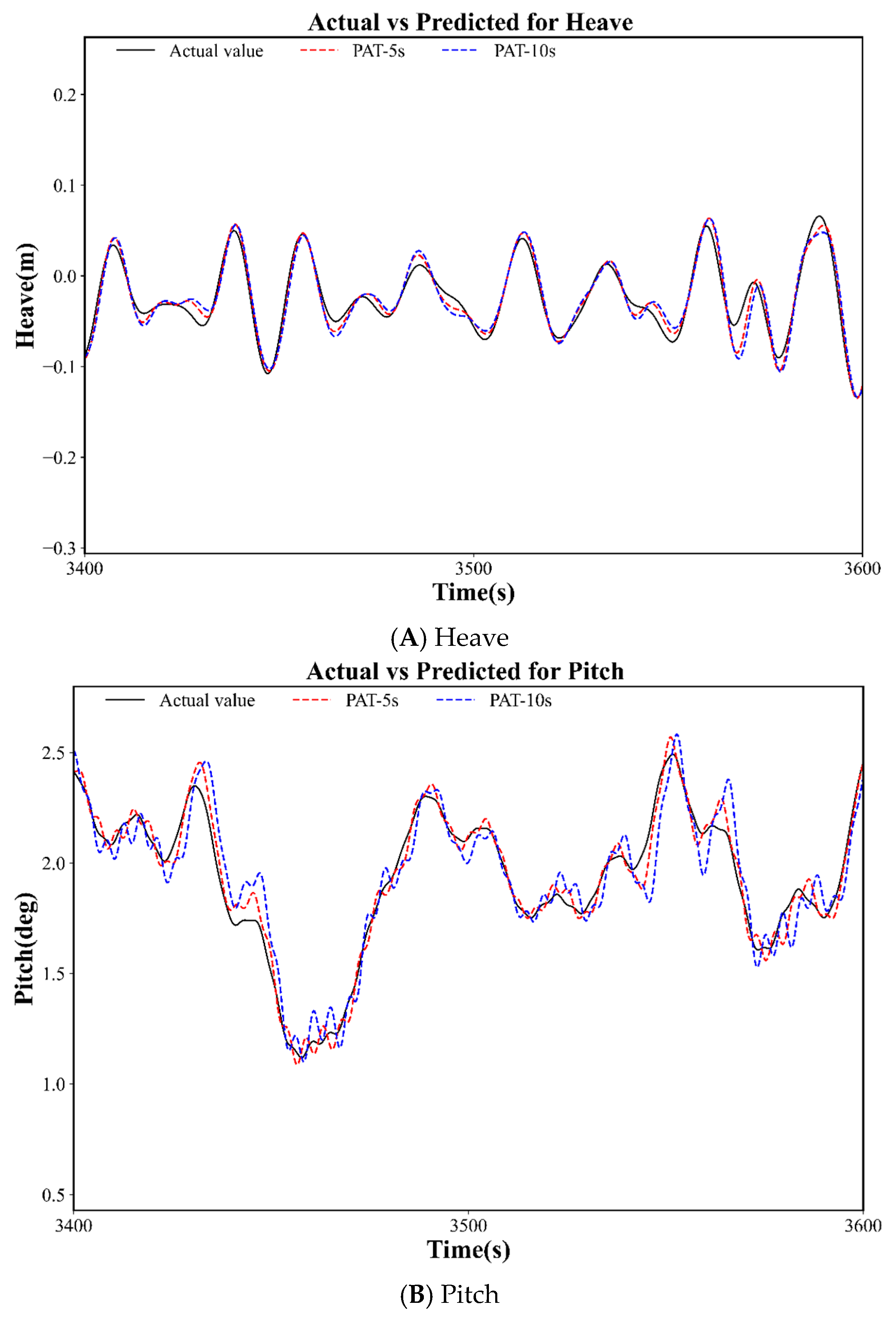
The PAT values are set to 5 s and 10 s, and the STL–TimesNet–NLinear model is trained under the EC1 condition to predict the 6-DOF motion responses. From the test set, portions of the heave and pitch data are randomly selected to visualize the prediction results, as shown in Figure 12. The black curves represent the actual test data, while the other curves show the model predictions under different PAT settings (5 s and 10 s). When the PAT is set to 5 s, the predicted responses of all 6-DOFs closely match the actual values, with particularly high accuracy at the peak and valley regions. It is evident that as the PAT increases, the deviation between the predicted and actual values gradually becomes larger. This is because the model must retain a greater amount of past information, while the growing influence of future uncertainties makes long-horizon prediction increasingly challenging. Nevertheless, the overall trends of the predicted responses remain highly consistent with the true data.

Figure 12. Predicted heave and pitch responses under different PAT settings for selected test samples.

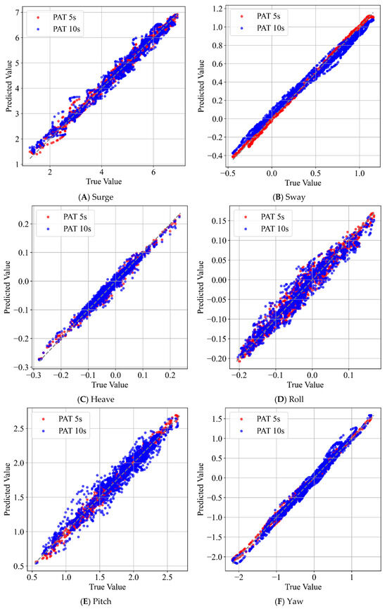
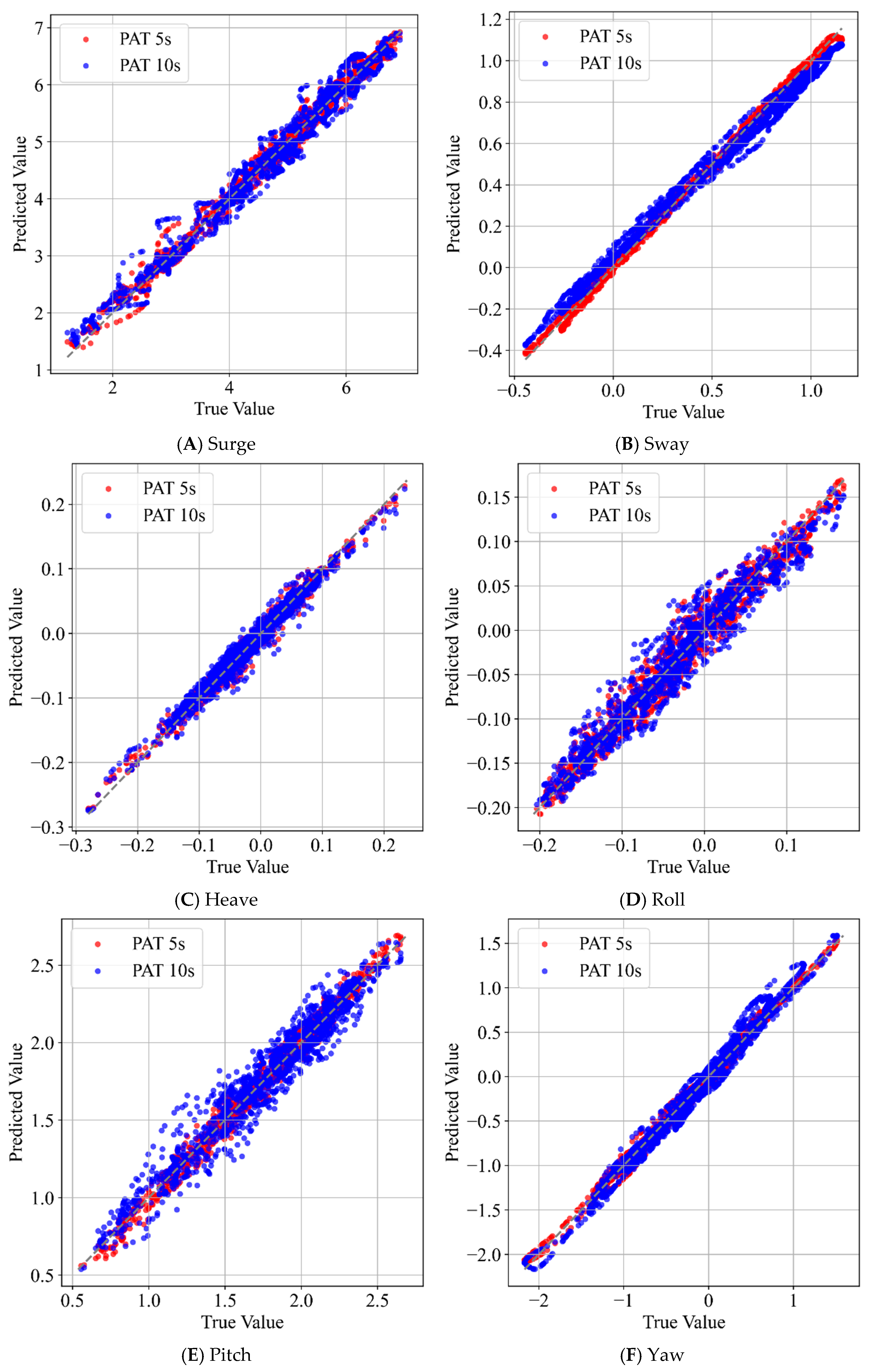
Figure 13 presents the scatter plots comparing the fitted predictions with the actual data, while Table 7 summarizes the prediction performance metrics of the 6-DOFs under the two PAT settings. As shown in Figure 12 and Figure 13 and Table 7, when the PAT is 5 s, all 6-DOFs exhibit low MAE values and demonstrate a high level of agreement with the true responses. The predicted results show minimal dispersion, and the R² values exceed 0.95, indicating that the model possesses strong capability in capturing the underlying trends of the time series. When the PAT increases to 10 s, the MAE values for the heave, pitch, and roll motions increase substantially, implying a decline in prediction accuracy and greater dispersion in the predicted responses. Nevertheless, the R² values remain above 0.90, suggesting that the overall trend-fitting performance is still acceptable despite the reduced accuracy and longer prediction horizon. For the surge, sway, and yaw motions, the decrease in prediction accuracy is relatively small. The predicted results remain low in dispersion, and the R² values consistently stay above 0.95, indicating that the predicted trends remain highly consistent with the actual data.

Figure 13. Scatter plots of STL–TimesNet–NLinear model predictions under different PATs.

Table 7. STL–TimesNet–NLinear models evaluation metrics under different PATs.

PAT	Metrics	Surge	Sway	Heave	Roll	Pitch	Yaw
5 s	MAE	0.1033	0.0172	0.0072	0.0121	0.0394	0.0491
	RMSE	0.1310	0.0217	0.0091	0.0155	0.0495	0.0599
	R2	0.9913	0.9979	0.9837	0.9671	0.9873	0.9937
10 s	MAE	0.1647	0.0571	0.0099	0.0162	0.0816	0.0822
	RMSE	0.2081	0.0629	0.0126	0.0207	0.1045	0.1028
	R2	0.9779	0.9822	0.9690	0.9411	0.9437	0.9814

Overall, an increase in PAT leads to reduced prediction accuracy because the model must retain more historical information, weakening certain temporal dependencies, while error accumulation becomes more prominent as the prediction horizon extends. Despite these challenges, the proposed model continues to demonstrate high predictive accuracy and strong practical applicability.

4.3. Comparison Among Different Environmental Conditions

To comprehensively evaluate the predictive performance of the STL–TimesNet–NLinear model under different environmental conditions (ECs), experiments were conducted for EC2 and EC3, as summarized in Table 8. The prediction results under both conditions demonstrate the strong capability and favorable generalization stability of the STL–TimesNet–NLinear model in short-term forecasting of FOWTs motion responses. For both environmental conditions, the model achieves its best performance when the PAT is set to 5 s, yielding low MAE and RMSE values as well as high R² scores across all 6-DOFs. Notably, the R² values for sway and yaw exceed 0.99 under both EC2 and EC3, indicating excellent trend-tracking capability and robust numerical fitting.

Table 8. STL–TimesNet–NLinear models evaluation metrics under EC2 and EC3.

	PAT	Metrics	Surge	Sway	Heave	Roll	Pitch	Yaw
EC2	5 s	MAE	0.1596	0.0310	0.0080	0.0240	0.0987	0.0783
		RMSE	0.2008	0.0398	0.0101	0.0305	0.1241	0.0971
		R2	0.9855	0.9969	0.9890	0.9608	0.9763	0.9918
	10 s	MAE	0.2155	0.0629	0.0131	0.0305	0.1527	0.1224
		RMSE	0.2709	0.0717	0.0165	0.0388	0.1913	0.1504
		R2	0.9737	0.9900	0.9705	0.9366	0.9437	0.9803
EC3	5 s	MAE	0.2031	0.0365	0.0139	0.0322	0.1236	0.0990
		RMSE	0.2553	0.0464	0.0177	0.0411	0.1571	0.1229
		R2	0.9826	0.9904	0.9833	0.9676	0.9745	0.9906
	10 s	MAE	0.2764	0.0572	0.0204	0.0402	0.1882	0.1212
		RMSE	0.3458	0.0705	0.0259	0.0512	0.2401	0.1613
		R2	0.9681	0.9777	0.9641	0.9497	0.9405	0.9839

When the PAT is increased to 10 s, a gradual decline in prediction accuracy is observed. Among the 6-DOFs, surge, heave, and pitch exhibit the most pronounced degradation due to their stronger sensitivity to wind–wave excitation and inherently nonlinear dynamics, leading to larger error growth. In contrast, sway and yaw maintain strong robustness, with only minor increases in MAE and RMSE and R² values still above 0.97. This reflects their intrinsic periodicity and relatively predictable dynamic characteristics.

A comparison between EC2 and EC3 further indicates that the latter introduces stronger environmental disturbances, resulting in slightly higher error levels. Nevertheless, the overall predictive trends remain consistent, and the R² values for all DOFs remain above 0.94 even at longer PAT settings. These results suggest that although extending the prediction horizon inevitably reduces numerical accuracy, the STL–TimesNet–NLinear model retains stable trend-fitting capability and reliable generalization across varying sea states. This robustness highlights its practical value for motion prediction and engineering applications in floating wind turbine systems.

4.4. Overall Comparative Analysis

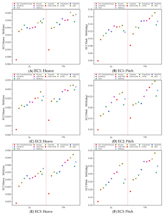
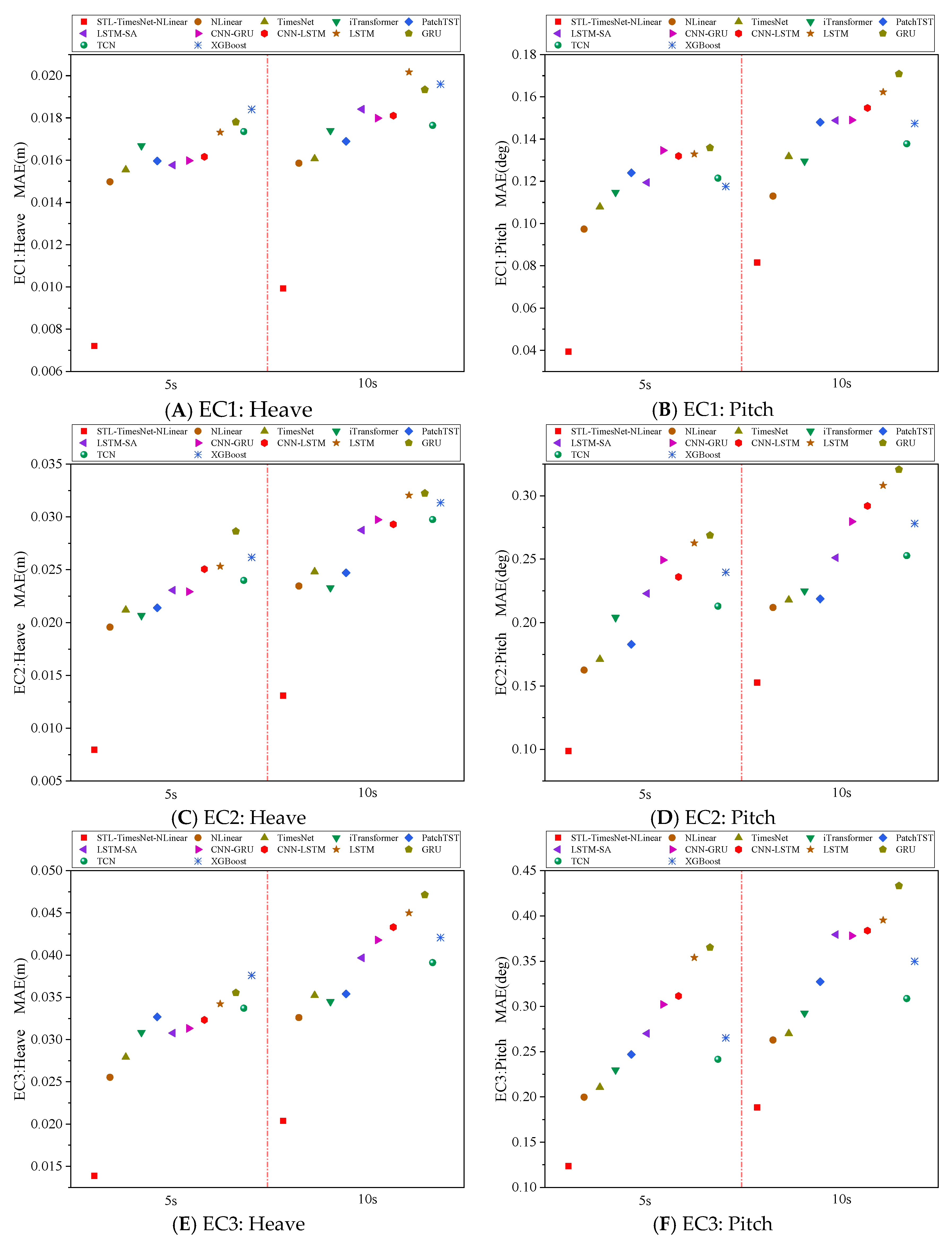
The MAE serves as a metric to measure the average magnitude of errors between the model-generated estimates and the observed ground truth. Minimizing the MAE value implies an increased level of consistency between the forecasted results and actual data, thereby demonstrating better results in numerical convergence and predictive fidelity. Figure 14 presents the MAE scatter plots of heave and pitch motions for the STL–TimesNet–NLinear model and the benchmark models under the EC1–EC3 conditions at PAT = {5 s, 10 s}. In the figure, the horizontal axis is divided into two segments by a red dashed line, corresponding to PAT = 5 s and PAT = 10 s, while the vertical axis represents the MAE. The results clearly show that the proposed model consistently achieves the lowest MAE across all PAT values, demonstrating superior prediction accuracy and a closer alignment with the true data compared with the baseline models.

Figure 14. Comparison of heave and pitch MAE among different models under EC1–EC3.

For instance, in the heave motion, relative to the second-best-performing model, the MAE is reduced by 51.9%, 59.3%, and 45.7% under the three environmental conditions when PAT = 5 s. When PAT increases to 10 s, the reductions remain substantial, reaching 37.4%, 43.8%, and 37.5%, respectively. These findings further confirm the outstanding predictive capability of the STL–TimesNet–NLinear model and underscore its practical value for engineering applications.

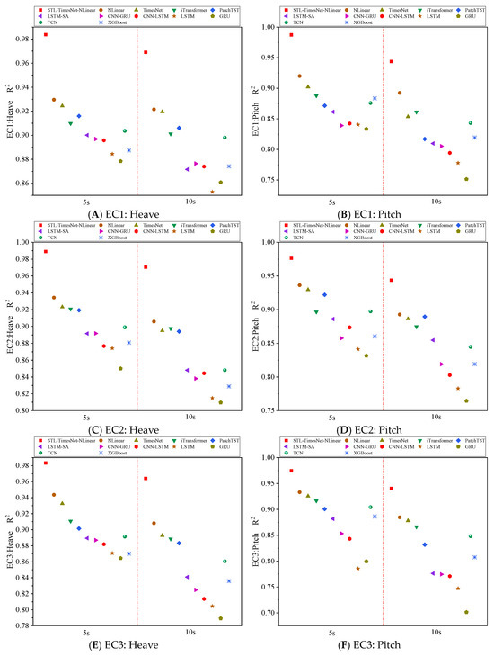
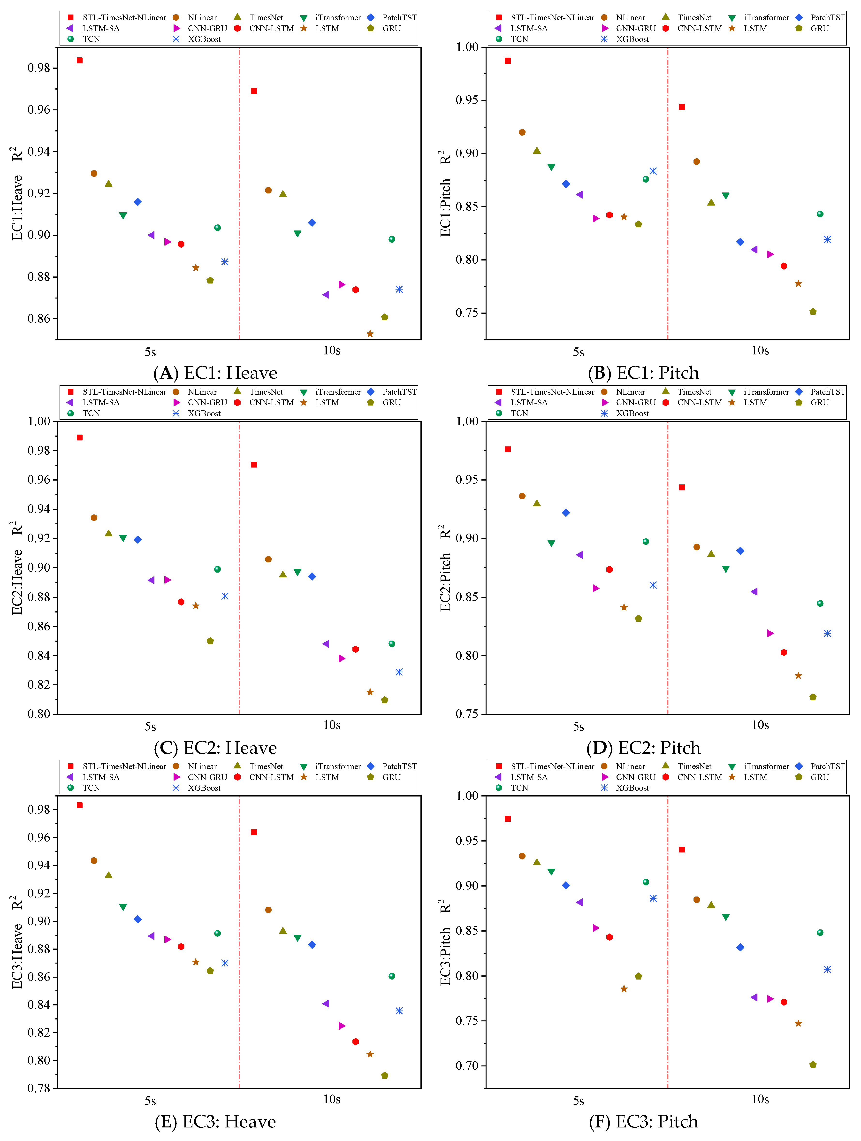
Figure 15 compares the R² scatter plots of heave and pitch motions at PAT = {5 s, 10 s}. The results show that under all environmental conditions, the STL–TimesNet–NLinear model consistently delivers the best predictive performance, with R² values surpassing those of all benchmark models. This demonstrates its strong capability in capturing the overall temporal trends of long motion sequences. When PAT = 5 s, the model achieves R² values above 0.98 for heave, substantially higher than the majority of RNN-based models, which generally fall below 0.90. For pitch motion, its R² remains above 0.95 across all ECs.

Figure 15. Comparison of heave and pitch R² among different models under EC1–EC3.

As PAT increases, the memory burden of the sequence becomes more demanding, leading to a noticeable degradation in prediction accuracy for all models. The decline is particularly pronounced for pitch, indicating that this degree of freedom exhibits stronger fluctuations and more complex dependency patterns, thereby imposing greater modeling challenges. Despite this degradation, the STL–TimesNet–NLinear model maintains R² values above 0.90 under all conditions, highlighting its superior robustness and adaptability.

In summary, experiments conducted under various environmental conditions and multiple PAT settings verify the feasibility and superiority of the proposed STL–TimesNet–NLinear model for short-term motion response prediction of FOWTs. Time-series data typically exhibit periodic and trending characteristics, and STL effectively decomposes the underlying seasonal and trend components. By integrating TimesNet and NLinear for joint prediction, the framework leverages the complementary strengths of both models, thereby enhancing prediction accuracy while maintaining high interpretability.

Furthermore, models such as iTransformer, PatchTST, TimesNet, and NLinear, which represent state-of-the-art approaches in time-series forecasting, demonstrate significantly higher prediction accuracy compared with RNN-based models, as well as the XGBoost and TCN models. This suggests that these advanced architectures hold substantial potential for future research on short-term motion response prediction of FOWTs.

4.5. Ablation Experiment

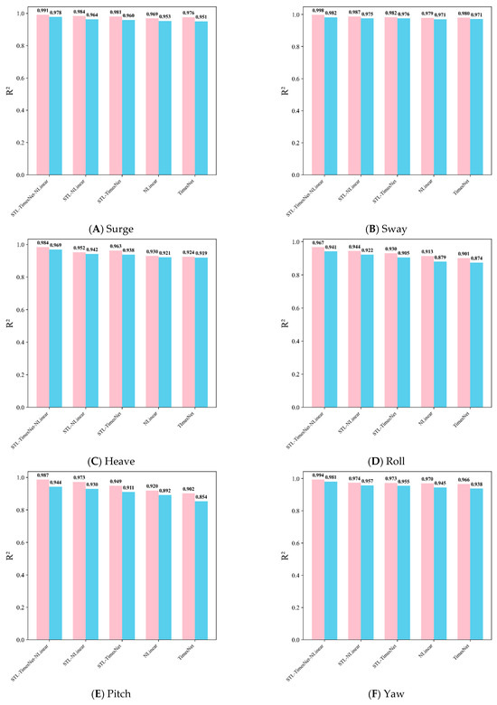
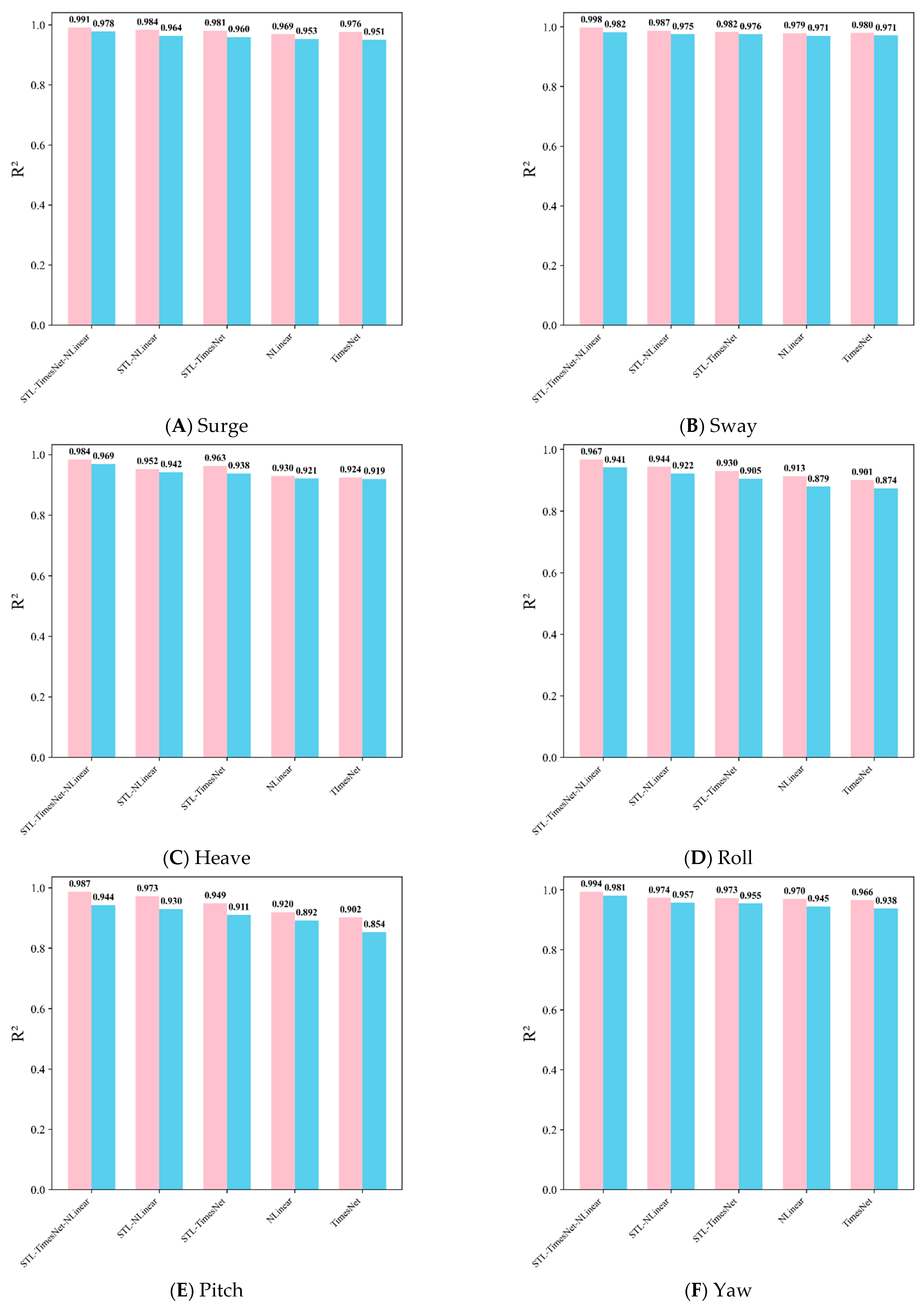
The ablation study comprehensively evaluates the six-degree-of-freedom motion prediction performance of five model architectures—STL–TimesNet–NLinear, STL–NLinear, STL–TimesNet, NLinear, and TimesNet—under the EC1 condition at PAT values of 5 s and 10 s, as summarized in Table 9 and illustrated in Figure 16. In Figure 16, pink represents the results for PAT = 5 s, while blue represents the results for PAT = 10 s. The results clearly demonstrate that STL–TimesNet–NLinear consistently achieves the highest prediction accuracy and strongest stability, outperforming all other models in terms of MAE, RMSE, and R². For horizontal motions (surge and sway), STL–TimesNet–NLinear exhibits markedly lower errors and higher R² scores, indicating a superior capability to capture both long-term drift components and small-amplitude lateral fluctuations. Its R² values for surge reach 0.9913 (5 s) and 0.9779 (10 s), while sway achieves near-perfect fitting with R² of 0.9979 and 0.9822, respectively, substantially surpassing the alternative variants. In the vertical heave motion, the model maintains exceptional accuracy, with MAE and RMSE values significantly lower than those of the other models and R² consistently above 0.96. This highlights its robustness in modeling low-energy vertical responses where both trend decomposition and multi-scale temporal representation are essential.

Table 9. Evaluation metrics of different models after the ablation experiments.

Models		STL–TimesNet–NLinear		STL–NLinear		STL–TimesNet		NLinear		TimesNet
Metrics		MAE	RMSE	MAE	RMSE	MAE	RMSE	MAE	RMSE	MAE	RMSE
Surge	5 s	0.1033	0.1310	0.1429	0.1796	0.1568	0.1952	0.1917	0.2476	0.1665	0.2152
	10 s	0.1647	0.2081	0.2130	0.2662	0.2275	0.2805	0.2409	0.3023	0.2477	0.3101
Sway	5 s	0.0172	0.0217	0.0419	0.0529	0.0476	0.0626	0.0489	0.0683	0.0485	0.0675
	10 s	0.0571	0.0629	0.0523	0.0742	0.0550	0.0736	0.0636	0.0808	0.0642	0.0800
Heave	5 s	0.0072	0.0091	0.0123	0.0157	0.0109	0.0138	0.0150	0.0190	0.0156	0.0197
	10 s	0.0099	0.0126	0.0136	0.0173	0.0141	0.0178	0.0159	0.0201	0.0161	0.0203
Roll	5 s	0.0121	0.0155	0.0159	0.0202	0.0176	0.0225	0.0197	0.0251	0.0211	0.0268
	10 s	0.0162	0.0207	0.0186	0.0237	0.0206	0.0262	0.0232	0.0296	0.0238	0.0303
Pitch	5 s	0.0394	0.0495	0.0574	0.0730	0.0777	0.0995	0.0974	0.1245	0.1079	0.1378
	10 s	0.0816	0.1045	0.0910	0.1164	0.1029	0.1314	0.1130	0.1444	0.1318	0.1685
Yaw	5 s	0.0491	0.0599	0.0970	0.1229	0.0946	0.1237	0.0970	0.1311	0.1021	0.1394
	10 s	0.0822	0.1028	0.1132	0.1558	0.1224	0.1610	0.1365	0.1774	0.1459	0.1887

Figure 16. R² values of different models after the ablation experiments.

In the rotational degrees of freedom (roll, pitch, and yaw), STL–TimesNet–NLinear again delivers the strongest performance. Its R² for roll and pitch substantially exceeds those of the other models, reflecting its ability to accurately capture the complex nonlinear and multi-frequency characteristics inherent in platform rotational dynamics. Pitch, which is typically the most challenging response due to strong aero-hydro-servo coupling, shows notable improvement, with the proposed model achieving R² values of 0.9873 (5 s) and 0.9437 (10 s), outperforming TimesNet by more than 9%. Yaw predictions also benefit from the hybrid architecture, with R² reaching 0.9937 and 0.9814 for the two PAT conditions, demonstrating enhanced robustness under more stochastic heading variations.

Overall, the results confirm that the joint introduction of STL decomposition, multi-scale temporal modeling from TimesNet, and linear residual constraints from NLinear produces significant complementary effects. This synergistic architecture not only reduces noise and preserves long-term trends but also improves the model’s capacity to learn nonlinear temporal dependencies and suppress extrapolation errors. Consequently, STL–TimesNet–NLinear stands out as the most effective and reliable configuration. The ablation study conclusively validates that each component contributes meaningfully to the final performance, and their integration enables the proposed model to provide highly accurate, stable, and generalizable short-term motion predictions for floating offshore wind turbines.

4.6. Generalization Analysis on 15 MW Windcrete Spar-Type FOWT

To further evaluate the FWT platform-type adaptability of the proposed STL–TimesNet–NLinear framework, a larger 15 MW Windcrete Spar-type FOWT was introduced as a second benchmark. This model is based on the IEA 15 MW reference wind turbine mounted on the Windcrete Spar platform, as defined in IEA Wind Task 37 [45] and the COREWIND project [46]. Compared to the 5 MW OC4 semi-submersible platform, the Windcrete concept features a monolithic concrete Spar structure with a significantly deeper draft (155 m) and low-frequency hydrodynamic responses. The key structural and inertial properties of the 15 MW Windcrete FOWT are summarized in Table 10.

Table 10. Summary properties of the 15 MW Windcrete Spar-type FOWT.

Item	Value
Rated power	15 MW
Rotor orientation	Upwind, 3 blades
Cut-in/Rated/Cut-out wind speeds	3 m/s, 10.59 m/s, 25 m/s
Rotor mass	195,000 kg
Nacelle mass	821,000 kg
Tower mass (Concrete)	1,263,000 kg
Hub height	135 m
Platform mass (including ballast)	36,550,000 kg
Center of Mass (CM) Height	−113.08 m
Platform draft	155 m
Platform roll/pitch inertia about CM	1.554 × 1011 kg·m2
Platform yaw inertia about CM	1.903 × 109 kg·m2

Furthermore, to verify the model’s performance under different load conditions, two additional environmental conditions (EC4 and EC5) were evaluated for the 15 MW platform, as shown in Table 11. EC4 represents a rated operational condition. EC5 simulates a parked (survival) scenario under extreme sea states.

Table 11. Parameters of two Environmental conditions.

Item	${\mathit{u}}_{\mathit{h}\mathit{u}\mathit{b}}$	${\mathit{H}}_{\mathit{s}}$	${\mathit{T}}_{\mathit{p}}$	Peak-Shape Parameter	Operational Status
EC4	10.5 m/s	5.11 m	11 s	3.3	Operation
EC5	38 m/s	6.3 m	13.5 s	3.3	Parked

Table 12 compares the performance of the STL–TimesNet–NLinear model against several benchmark approaches on the 15 MW Windcrete Spar-type platform at a PAT of 5 s. As illustrated, the proposed model consistently achieves better predictive accuracy across all 6-DOFs under both operational (EC4) and extreme (EC5) scenarios. Specifically, for the critical pitch and surge motions in EC4, the model gave high R² values of 0.9817 and 0.9886, respectively. These results underscore the framework’s capability to capture multi-periodic characteristics in 15 MW-class turbines. Compared with both state-of-the-art time-series models and traditional RNN-based architectures, the proposed framework exhibits better performances. In the pitch motion under EC4, the STL–TimesNet–NLinear model achieves a reduction of 49.7% in MAE and 48.8% in RMSE compared to the second-best-performing baseline (NLinear), while the R² increases by 5.5%. The performance gain over the traditional LSTM is even more substantial: the MAE for pitch is decreased by 67.8%, with the R² increasing from a moderate 0.8240 to an excellent 0.9817. Furthermore, in heave motion, the model achieves a 52.7% reduction in both MAE and RMSE relative to the NLinear model. Notably, even under the extreme non-stationary conditions of EC5, the framework maintains its better performance. For the pitch motion under this survival sea state, it reduces the MAE by 31.9% compared to NLinear, and by 54.7% compared to the traditional LSTM, while increasing the R² from 0.7903 (LSTM) to 0.9573. Overall, the framework maintains R² values exceeding 0.94 for all 6-DOFs under EC5. The consistent better performance of the STL–TimesNet–NLinear model across the two different turbine sizes (5 MW and 15 MW) and platform typologies (Semi-submersible and Spar) validates its applicability for the short-term motion response prediction of FOWTs.

Table 12. Prediction evaluation metrics for different models.

	Models	STL–TimesNet–NLinear			NLinear			iTransformer			LSTM-SA			LSTM
	Metrics	MAE	RMSE	R2	MAE	RMSE	R2	MAE	RMSE	R2	MAE	RMSE	R2	MAE	RMSE	R2
EC4	Surge	0.1464	0.1876	0.9886	0.2516	0.3174	0.9674	0.3212	0.4032	0.9474	0.3740	0.4687	0.9289	0.4291	0.5377	0.9064
	Sway	0.0607	0.0734	0.9849	0.0912	0.1115	0.9652	0.0926	0.1083	0.9672	0.1257	0.1522	0.9353	0.1305	0.1608	0.9277
	Heave	0.0204	0.0253	0.9841	0.0431	0.0535	0.9288	0.0479	0.0594	0.9121	0.0525	0.0652	0.8941	0.0574	0.0713	0.8737
	Roll	0.0334	0.0485	0.9797	0.0559	0.0850	0.9376	0.0663	0.1002	0.9134	0.0752	0.1145	0.8870	0.0849	0.1298	0.8546
	Pitch	0.0723	0.0926	0.9817	0.1436	0.1809	0.9301	0.1676	0.2188	0.8977	0.1924	0.2448	0.8720	0.2247	0.2870	0.8240
	Yaw	0.0417	0.0556	0.9893	0.0711	0.0929	0.9701	0.0839	0.1066	0.9606	0.1055	0.1370	0.9349	0.1149	0.1489	0.9232
EC5	Surge	0.1440	0.1822	0.9617	0.2055	0.2582	0.9231	0.2281	0.2866	0.9053	0.2620	0.3291	0.8752	0.2972	0.3734	0.8393
	Sway	0.0014	0.0017	0.9667	0.0019	0.0023	0.9420	0.0021	0.0025	0.9281	0.0022	0.0027	0.9205	0.0024	0.0028	0.9109
	Heave	0.0404	0.0528	0.9664	0.0660	0.0849	0.9129	0.0712	0.0914	0.8990	0.0791	0.1007	0.8776	0.0857	0.1088	0.8571
	Roll	0.0008	0.0010	0.9498	0.0010	0.0013	0.9170	0.0012	0.0016	0.8705	0.0014	0.0017	0.8424	0.0014	0.0018	0.8308
	Pitch	0.0545	0.0683	0.9573	0.0800	0.1003	0.9079	0.0936	0.1176	0.8735	0.1078	0.1357	0.8315	0.1204	0.1514	0.7903
	Yaw	0.0017	0.0023	0.9801	0.0025	0.0032	0.9609	0.0033	0.0041	0.9343	0.0040	0.0052	0.8967	0.0042	0.0055	0.8844

5. Concluding Remarks

To address the practical demand for high-accuracy short-term motion prediction of floating offshore wind turbines (FOWTs) operating in complex marine environments, this study proposes a novel decomposition-enhanced forecasting framework, STL–TimesNet–NLinear. The framework integrates the STL seasonal-trend decomposition method with the multi-period time-series modeling capability of TimesNet and the long-term trend prediction capability of NLinear. The proposed model was numerically tested on two different platform typologies (a 5 MW semi-submersible and a 15 MW spar-type platform) and various operational conditions. Furthermore, an ablation study was conducted to investigate the individual contributions and effectiveness of each component within the STL–TimesNet–NLinear framework. The main conclusions are summarized as follows:

(1)

By employing TimesNet for wave-frequency responses and NLinear for low-frequency drifts, the framework successfully captured seasonal and trend variations. Under standard conditions with a PAT of 5 s, the STL–TimesNet–NLinear model achieves the highest prediction accuracy across all 6-DOFs, reducing the MAE by 37.9–59.5% and the RMSE by 38.0–60.2% relative to the second-best-performing baseline model.

(2)

The framework demonstrates the ability to generalize when applied to the larger sized 15 MW Windcrete Spar-type platform. Specifically, under extreme environmental conditions, the framework reduces the MAE for pitch motion by 31.9% compared to the second-best-performing baseline model (NLinear). The performance improvement over the traditional LSTM model is also higher: the MAE for pitch is decreased by 54.7%, and the R² value increases from 0.7903 to 0.9573.

(3)

Although prediction accuracy naturally decreases as the PAT increases, the proposed model consistently keeps prediction errors at low levels. Across all experimental settings, the R² values remain above 0.94, significantly outperforming traditional RNN-based models. Moreover, the computational runtime is reduced by more than half compared to conventional RNN architectures, primarily because RNNs inherently rely on sequential processing. Additionally, the proposed model achieves an ultra-fast inference latency of only 2.4 ms per step, which is substantially lower than the 15.7 ms required by the GRU model.

(4)

The ablation study quantitatively confirms that incorporating STL significantly enhances model stability. Across all 6-DOFs, both STL–TimesNet and STL–NLinear consistently outperform their non-decomposed counterparts, with the proposed STL–TimesNet–NLinear model achieving the highest predictive accuracy. This demonstrates the complementary benefits of this physical “feature-to-model” alignment approach over conventional black-box and traditional RNN-based architectures.

While the proposed STL–TimesNet–NLinear framework demonstrates strong predictive accuracy across different FOWT platforms (e.g., the 5 MW and 15 MW models), several limitations remain that warrant future investigation. First, the current framework employs the STL method, which assumes a purely additive relationship between the trend and seasonal components. However, under extremely severe sea states, the aero-hydrodynamic coupling between low-frequency slow drifts and wave-frequency oscillations may exhibit strong non-additive (e.g., multiplicative or synergistic) nonlinearities, which an additive approach might oversimplify. Second, the model has been tested primarily through high-fidelity OpenFAST simulations, lacking verification with real-world offshore data that often contain noise, signal dropouts, and unmodeled disturbances. Additionally, although we included a modern 15 MW platform, the framework has not yet been comprehensively validated across the specific datasets and complex modeling conditions of the OC5–OC7 projects.

New algorithms in time-series forecasting are constantly emerging. Consequently, our future research will focus on developing adaptive, non-additive decomposition algorithms to handle extreme nonlinear coupling, and integrating Transfer Learning (TL) techniques to bridge the domain gap between numerical simulations and actual field measurements. We also plan to extend our validation to OC5–OC7 datasets and continuously benchmark our framework against future state-of-the-art models to allow for more comprehensive comparisons.

References

- McCoy, A.; Musial, W.; Hammond, R.; Mulas Hernando, D.; Duffy, P.; Beiter, P.; Pérez, P.; Baranowski, R.; Reber, G.; Spitsen, P. Offshore Wind Market Report: 2024 Edition (No. NREL/TP-5000-90525); National Renewable Energy Laboratory (NREL): Golden, CO, USA, 2024. [CrossRef] [Scilit]
- Yi, Y.; Sun, K.; Liu, Y.; Zhang, J.; Zhang, H.; Zhu, R.; Yao, H.D. Coupled numerical framework for wind-wave-to-wire energy conversion in floating hybrid wind-wave systems. Appl. Energy 2026, 403, 127106. [Google Scholar] [CrossRef] [Scilit]
- International Energy Agency. Renewables 2025; IEA: Paris, France, 2025; Available online: https://www.iea.org/reports/renewables-2025 (accessed on 19 January 2026).
- Ojo, A.; Collu, M.; Coraddu, A. Multidisciplinary design analysis and optimization of floating offshore wind turbine substructures: A review. Ocean Eng. 2022, 266, 112727. [Google Scholar] [CrossRef] [Scilit]
- Liu, Y.; Li, S.; Yi, Q.; Chen, D. Developments in semi-submersible floating foundations supporting wind turbines: A comprehensive review. Renew. Sustain. Energy Rev. 2016, 60, 433–449. [Google Scholar] [CrossRef] [Scilit]
- Koondhar, M.A.; Albsha, L.; Mahmoud, S.A.; Amin, L.G.; Mahariq, I. Comparative analysis of onshore, offshore, and floating wind turbines for renewable energy systems: A review. Ocean Eng. 2026, 343, 123243. [Google Scholar] [CrossRef] [Scilit]
- Stetco, A.; Dinmohammadi, F.; Zhao, X.; Robu, V.; Flynn, D.; Barnes, M.; Keane, J.; Nenadic, G. Machine learning methods for wind turbine condition monitoring: A review. Renew. Energy 2019, 133, 620–635. [Google Scholar] [CrossRef] [Scilit]
- Chuang, T.C.; Yang, W.H.; Yang, R.Y. Experimental and numerical study of a barge-type FOWT platform under wind and wave load. Ocean Eng. 2021, 230, 109015. [Google Scholar] [CrossRef] [Scilit]
- Jonkman, J.; Butterfield, S.; Musial, W.; Scott, G. Definition of a 5-MW Reference Wind Turbine for Offshore System Development (No. NREL/TP-500-38060); National Renewable Energy Laboratory (NREL): Golden, CO, USA, 2009. Available online: https://www.nrel.gov/docs/fy09osti/38060.pdf (accessed on 5 March 2026).
- Lackner, M.A.; Rotea, M.A. Structural control of floating wind turbines. Mechatronics 2011, 21, 704–719. [Google Scholar] [CrossRef] [Scilit]
- Yalla, S.K.; Kareem, A.; Kantor, J.C. Semi-active tuned liquid column dampers for vibration control of structures. Eng. Struct. 2001, 23, 1469–1479. [Google Scholar] [CrossRef] [Scilit]
- Chu, S.Y.; Soong, T.T.; Reinhorn, A.M. Active, Hybrid, and Semi-Active Structural Control: A Design and Implementation Handbook; Wiley: New York, NY, USA, 2005. [Google Scholar]
- Guo, X.; Zhang, X.; Lu, W.; Tian, X.; Li, X. Real-time prediction of 6-DOF motions of a turret-moored FPSO in harsh sea state. Ocean Eng. 2022, 265, 112500. [Google Scholar] [CrossRef] [Scilit]
- Wiener, N. Extrapolation, Interpolation, and Smoothing of Stationary Time Series: With Engineering Applications; The MIT Press: Cambridge, MA, USA, 1949. [Google Scholar] [CrossRef] [Scilit]
- Kaplan, P. A Preliminary Study of Prediction Techniques for Aircraft Carrier Motions at Sea (Report No. 65-22); Oceanics Inc.: Plainview, NY, USA, 1965. [Google Scholar]
- Qiao, D.; Li, P.; Ma, G.; Qi, X.; Yan, J.; Ning, D.; Li, B. Realtime prediction of dynamic mooring lines responses with LSTM neural network model. Ocean Eng. 2021, 219, 108368. [Google Scholar] [CrossRef] [Scilit]
- Yin, J.; Ding, J.; Yang, Y.; Yu, J.; Ma, L.; Xie, W.; Nie, D.; Bashir, M.; Liu, Q.; Li, C.; et al. Wave-induced motion prediction of a deepwater floating offshore wind turbine platform based on Bi-LSTM. Ocean Eng. 2025, 315, 119836. [Google Scholar] [CrossRef] [Scilit]
- Zhou, H.; Li, J.; Zhang, S.; Zhang, S.; Yan, M.; Xiong, H. Expanding the prediction capacity in long sequence time-series forecasting. Artif. Intell. 2023, 318, 103886. [Google Scholar] [CrossRef] [Scilit]
- Ye, Y.; Wang, L.; Wang, Y.; Qin, L. An EMD-LSTM-SVR model for the short-term roll and sway predictions of semi-submersible. Ocean Eng. 2022, 256, 111460. [Google Scholar] [CrossRef] [Scilit]
- Wei, Q.; Wu, B.; Li, X.; Guo, X.; Teng, Y.; Gong, Q.; Wang, S. Short-term motion prediction of a semi-submersible platform based on a combined prediction model. Ocean Eng. 2024, 307, 118039. [Google Scholar] [CrossRef] [Scilit]
- Deng, S.; Ning, D.; Mayon, R. The motion forecasting study of floating offshore wind turbine using self-attention long short-term memory method. Ocean Eng. 2024, 310, 118709. [Google Scholar] [CrossRef] [Scilit]
- Zhou, H.; Zhang, S.; Peng, J.; Zhang, S.; Li, J.; Xiong, H.; Zhang, W. Informer: Beyond efficient transformer for long sequence time-series forecasting. In Proceedings of the AAAI Conference on Artificial Intelligence 2021, Virtually, 2–9 February 2021; Volume 35, pp. 11106–11115. [Google Scholar] [CrossRef] [Scilit]
- Wu, H.; Xu, J.; Wang, J.; Long, M. Autoformer: Decomposition transformers with auto-correlation for long-term series forecasting. arXiv 2021, arXiv:2106.13008. [Google Scholar] [CrossRef] [Scilit]
- Zhou, T.; Ma, Z.; Wen, Q.; Wang, X.; Sun, L.; Jin, R. FEDformer: Frequency enhanced decomposed transformer for long-term series forecasting. In Proceedings of the International Conference on Machine Learning; PMLR: Baltimore, MD, USA, 2022; pp. 27268–27286. [Google Scholar] [CrossRef] [Scilit]
- Nie, Y.; Nguyen, N.H.; Sinthong, P.; Kalagnanam, J. A time series is worth 64 words: Long-term forecasting with transformers. arXiv 2022, arXiv:2211.14730. [Google Scholar] [CrossRef] [Scilit]
- Wu, H.; Hu, T.; Liu, Y.; Zhou, H.; Wang, J.; Long, M. TimesNet: Temporal 2d-variation modeling for general time series analysis. arXiv 2022, arXiv:2210.02186. [Google Scholar] [CrossRef] [Scilit]
- Liu, Y.; Hu, T.; Zhang, H.; Wu, H.; Wang, S.; Ma, L.; Long, M. iTransformer: Inverted transformers are effective for time series forecasting. arXiv 2023, arXiv:2310.06625. [Google Scholar] [CrossRef] [Scilit]
- Zeng, A.; Chen, M.; Zhang, L.; Xu, Q. Are transformers effective for time series forecasting? Proc. AAAI Conf. Artif. Intell. 2023, 37, 11121–11128. [Google Scholar] [CrossRef] [Scilit]
- Wang, H.K.; Song, K.; Cheng, Y. A hybrid forecasting model based on CNN and informer for short-term wind power. Front. Energy Res. 2022, 9, 788320. [Google Scholar] [CrossRef] [Scilit]
- Deng, F.; Wang, J.; Wu, L.; Gao, B.; Wei, B.; Li, Z. Distributed photovoltaic power forecasting based on personalized federated adversarial learning. Sustain. Energy Grids Netw. 2024, 40, 101537. [Google Scholar] [CrossRef] [Scilit]
- Wang, J.; Jiang, W.; Shu, S.; He, X. A multi-factor clustering integration paradigm for wind speed point-interval prediction based on feature selection and optimized inverted transformer. Energy 2025, 320, 135210. [Google Scholar] [CrossRef] [Scilit]
- Hu, F.; Zhang, X.; Cheng, Y.; Ling, H.; Dou, P.; Zhang, P.; Xing, Y.; Xu, X.; Wang, S. Multi-period modeling of floating production storage and offloading dock mooring line tensions using TimesNet-based deep learning framework. Ocean Eng. 2026, 353, 124651. [Google Scholar] [CrossRef] [Scilit]
- Gong, J.; Qu, Z.; Zhu, Z.; Xu, H. Parallel TimesNet-BiLSTM model for ultra-short-term photovoltaic power forecasting using STL decomposition and auto-tuning. Energy 2025, 320, 135286. [Google Scholar] [CrossRef] [Scilit]
- Qiu, X.; Hu, J.; Zhou, L.; Wu, X.; Du, J.; Zhang, B.; Guo, C.; Zhou, A.; Jensen, C.S.; Sheng, Z.; et al. TFB: Towards comprehensive and fair benchmarking of time series forecasting methods. arXiv 2024, arXiv:2403.20150. [Google Scholar] [CrossRef] [Scilit]
- Cleveland, R.B.; Cleveland, W.S.; McRae, J.E.; Terpenning, I. STL: A seasonal-trend decomposition procedure based on loess. J. Off. Stat. 1990, 6, 3–73. [Google Scholar]
- Szegedy, C.; Liu, W.; Jia, Y.; Sermanet, P.; Reed, S.; Anguelov, D.; Erhan, D.; Vanhoucke, V.; Rabinovich, A. Going deeper with convolutions. In Proceedings of the IEEE Conference on Computer Vision and Pattern Recognition, Boston, MA, USA, 7–12 June 2015; IEEE: New York, NY, USA, 2015; pp. 1–9. [Google Scholar] [CrossRef] [Scilit]
- Robertson, A.; Jonkman, J.; Masciola, M.; Song, H.; Goupee, A.; Coulling, A.; Luan, C. Definition of the Semisubmersible Floating System for Phase II of OC4 (Technical Report No. NREL/TP-5000-60601); National Renewable Energy Laboratory (NREL): Golden, CO, USA, 2014. Available online: https://www.nrel.gov/docs/fy14osti/60601.pdf (accessed on 19 January 2026).
- Robertson, A.N.; Wendt, F.; Jonkman, J.M.; Popko, W.; Dagher, H.; Gueydon, S.; Qvist, J.; Vittori, F.; Azcona, J.; Uzunoglu, E.; et al. OC5 project phase II: Validation of global loads of the DeepCwind floating semisubmersible wind turbine. Energy Procedia 2017, 137, 38–57. [Google Scholar] [CrossRef] [Scilit]
- Robertson, A.N.; Gueydon, S.; Bachynski, E.; Wang, L.; Jonkman, J.; Alarcon, D.; Amet, E.; Beardsell, A.; Bonnet, P.; Boudet, B.; et al. OC6 Phase I: Investigating the underprediction of low-frequency hydrodynamic loads and responses of a floating wind turbine. J. Phys. Conf. Ser. 2020, 1618, 032033. [Google Scholar] [CrossRef] [Scilit]
- Wendt, F.F.; Robertson, A.N.; Jonkman, J.M. FAST model calibration and validation of the OC5-DeepCwind floating offshore wind system against wave tank test data. Int. J. Offshore Polar Eng. 2019, 29, 15–23. [Google Scholar] [CrossRef] [Scilit]
- DNV-ST-0437; Loads and Site Conditions for Wind Turbines. Høvik: Bærum, Norway, 2024. Available online: https://www.dnv.com/energy/standards-guidelines/dnv-st-0437-loads-and-site-conditions-for-wind-turbines/ (accessed on 19 January 2026).
- Shi, W.; Hu, L.; Lin, Z.; Zhang, L.; Wu, J.; Chai, W. Short-term motion prediction of floating offshore wind turbine based on muti-input LSTM neural network. Ocean Eng. 2023, 280, 114558. [Google Scholar] [CrossRef] [Scilit]
- Guo, X.; Zhang, X.; Tian, X.; Lu, W.; Li, X. Probabilistic prediction of the heave motions of a semi-submersible by a deep learning model. Ocean Eng. 2022, 247, 110578. [Google Scholar] [CrossRef] [Scilit]
- Herzen, J.; Lässig, F.; Piazzetta, S.G.; Neuer, T.; Tafti, L.; Raille, G.; Van Pottelbergh, T.; Pasieka, M.; Skrodzki, A.; Huguenin, N.; et al. Darts: User-friendly modern machine learning for time series. J. Mach. Learn. Res. 2022, 23, 5442–5447. Available online: http://jmlr.org/papers/v23/21-1177.html (accessed on 5 March 2026).
- Gaertner, E.; Sethuraman, L.; Anderson, B.; Barter, G.; Abbas, N.; Bortolotti, P.; Scott, G.; Feil, R.; Shields, M.; Rinker, J.; et al. IEA Wind TCP Task 37: Definition of the IEA 15-Megawatt Offshore Reference Wind Turbine (Technical Report No. NREL/TP-5000-75669); National Renewable Energy Laboratory (NREL): Golden, CO, USA, 2020. [CrossRef] [Scilit]
- Mahfouz, M.Y.; Molins, C.; Trubat, P.; Hernández, S.; Vigara, F.; Pegalajar-Jurado, A.; Bredmose, H.; Salari, M. Response of the International Energy Agency (IEA) Wind 15 MW WindCrete and Activefloat floating wind turbines to wind and second-order waves. Wind Energy Sci. 2021, 6, 867–883. [Google Scholar] [CrossRef] [Scilit]
Disclaimer/Publisher’s Note: The statements, opinions and data contained in all publications are solely those of the individual author(s) and contributor(s) and not of MDPI and/or the editor(s). MDPI and/or the editor(s) disclaim responsibility for any injury to people or property resulting from any ideas, methods, instructions or products referred to in the content. |
© 2026 by the authors. Licensee MDPI, Basel, Switzerland. This article is an open access article distributed under the terms and conditions of the Creative Commons Attribution (CC BY) license.