


Abstract
The Mexican Tropical Pacific (MTP) is a key component of the Eastern Tropical North Pacific Oxygen Minimum Zone, yet its carbonate system variability remains poorly constrained. This study examines wind-driven circulation effects on dissolved oxygen (DO) and the carbonate system —dissolved inorganic carbon (DIC), total alkalinity (TA), total-scale pH (pHT), partial pressure of CO2 in seawater (pCO2w) and air–sea CO2 fluxes (FCO2)— in the Gulf of Tehuantepec (GT) and Tehuantepec Bowl (TB). Hydrographic data and discrete water samples were collected at 50 oceanographic stations during March 2020. Principal Component Analysis (PCA) identifies wind-driven circulation as the primary control of biogeochemical variability. Tehuano wind events and mesoscale eddies promoted upwelling of low-oxygen (DO < 20 µmol kg−1) and high-DIC (>2200 µmol kg−1) waters to 50 m depth in the central GT, while downwelling conditions prevailed in the TB. Stoichiometric analysis revealed DIC-DO coupling (slope = −1.39). Overall, the MTP acted as CO2 source (FCO2 ranging from −1.92 to 24.11 mmol m−2 d−1), with enhanced emissions linked to eddy-induced upwelling. This study provides the first integrated characterization of the carbonate system across both the GT and TB.
1. Introduction
In the world’s oceans, regions of persistent hypoxia (DO < 20 µmol kg−1), known as Oxygen Minimum Zones (OMZs), have been identified in the eastern North Pacific, the eastern South Pacific, the Arabian Sea, and the Bay of Bengal [1,2]. In these zones, significant remineralization of organic matter under limited ventilation conditions results not only in a marked reduction in dissolved oxygen (DO) but also in the accumulation of dissolved inorganic carbon (DIC) and a decrease in pH [3,4]. This close coupling between oxygen depletion and carbon accumulation has led to these regions also being referred to as Carbonate Maximum Zones (CMZs) [5], highlighting their relevance to ocean acidification and the marine carbon cycle [6].
Within this global context, the Eastern Tropical North Pacific (ETNP), which includes the Mexican Tropical Pacific (MTP), is considered one of the largest OMZs on the planet, in terms of both vertical extent and horizontal coverage [2,7,8]. This region should play a key role in the global biogeochemical system, as it would modulate carbon cycling processes and regulate ocean–atmosphere exchanges of greenhouse gases including CO2 as reported in other OMZs [4,9,10]. Observations in the OMZ of the study area document a strong vertical gradient in DO concentrations, with values below 19.5 µmol kg−1 (originally reported in µmol L−1) decreasing to 4.9 µmol kg−1 at its core [2,11]. The upper boundary of this low-oxygen layer can shoal to depths as shallow as ~60 m [2,12], while elevated DIC concentrations exceeding 2200 µmol kg−1 have been reported in the pelagic zone [4,13,14]. Together, these features emphasize the tight physical-biogeochemical coupling that characterizes the MTP.
From a regional perspective, the MTP can be divided into three major subregions with distinct dynamical characteristics. To the northwest lies the transition zone near Cabo Corrientes (covering ~4 × 10⁴ km2) [12,15,16]; in the central portion, the sinking region known as the Tehuantepec Bowl (TB; ~14 × 104 km2) [17,18], characterized by anticyclonic circulation and associated water-mass downwelling, which also hosts the core of the northeastern tropical Pacific OMZ [2,7]; and to the southeast, the Gulf of Tehuantepec (GT: ~8 × 10⁴ km2), a region characterized by intense “Tehuano” winds and frequent mesoscale activity that strongly modulate the spatial distribution of carbonate system variables [14,19].
The “Tehuano” winds arise from strong pressure gradients across the Isthmus of Tehuantepec. These gradients drive air masses through the Chivela Pass, generating intense wind jets that extend offshore over the GT and the adjacent Pacific [20,21,22,23]. Typical events last 3–4 days, with wind speeds of 10–20 m s−1 that may exceed 25 m s−1 and occur primarily between November and February [24]. These wind jets promote vertical mixing and Ekman pumping, inducing cyclonic circulation within the GT [25] and affecting areas up to ~400 km offshore. As a result, sea surface temperature can decrease by up to 8 °C, and the thermocline can shoal to depths shallower than 20 m [14,26,27]. Concurrently, anticyclonic circulation develops west of the GT in the TB, where convergence of Ekman transport deepens the thermocline through forced subsidence [19,28]. These processes have direct implications for the vertical redistribution of oxygen and carbonate system properties.
At the southeastern end of the MTP, circulation is further influenced by the Costa Rica Coastal Current (CRCC), which flows northwestward with average speeds of ~20 cm s−1 and transports exceeding 5 Sv [18,29]. Interaction with the anticyclonic circulation in the TB limits its northward penetration, diverting the current southwestward along the coast of Oaxaca before it eventually turns southward. Seasonal variability in the CRCC has been documented, with poleward flow from October to February and equatorward flow from April to August [30]. In addition, the Mexican Coastal Current is initially expressed as a subsurface (subthermocline) poleward flow in the GT and gradually reaches the surface near ~17° N, where local winds reinforce its transport and allow interaction with a branch of the California Current that recirculates toward the Gulf of California [27,31,32,33]. This complex circulation framework provides multiple pathways for the transport and transformation of biogeochemical properties.
The MTP, located between 12° N and 23° N, is a tropical-subtropical transition zone with complex physical dynamics [34]. Two large-scale ocean currents converge north of the MTP. The first is the California Current, whose tropical branch extends from approximately 23° N to 17° N and transports cold, dense waters of subarctic origin toward the equator. The second is the Mexican Coastal Current, a surface flow toward higher latitudes (between 15° and 21° N), which transports warm, less dense waters of tropical origin [16,32,35,36,37]. Meanwhile, in the south-central part of the MTP is the warm water pool of the Pacific, where the temperature is usually >28.5 °C due to the waters being exposed to sunlight for longer periods, and where the surface dynamics change in the Gulf of Tehuantepec (GT) during “Tehuano winds” events in the fall-winter season [17,23,38,39].
The biogeochemical importance of the MTP has been highlighted by the coexistence, within the upper 150 m of the water column of a shallow OMZ beneath the thermocline, a pronounced DIC maximum, and the upper limit of subtropical subsurface water [40]. These features are closely linked and can be brought toward the surface by mesoscale processes such as coastal upwelling and cyclonic eddies. Consequently, regions such as the Gulf of Tehuantepec act as significant sources of CO2 to the atmosphere, with reported fluxes reaching 42 mmol m−2 d−1 [14]. However, despite this recognized importance, the spatial variability of the carbonate system and its coupling with oxygen dynamics remain incompletely resolved across large portions of the MTP.
In this context, the present study focuses on a region encompassing part of the OMZ core, the Tehuantepec Bowl, and the Gulf of Tehuantepec (~13.42–16.91° N and ~92.62–101.10° W), based on observations collected during an oceanographic cruise conducted in March 2020. Although the Mexican Tropical Pacific has been identified as biogeochemically significant, extensive areas between Acapulco (16.85° N, 99.90° W), Guerrero, and Puerto Escondido (15.87° N, 97.08° W), Oaxaca, remain poorly characterized in terms of carbonate system variability, having been sampled only sporadically or during isolated campaigns [41] of lower spatial resolution, especially in the region between 98° W and 102° W. This study addresses this spatial gap by providing a regional characterization of the carbonate system across this understudied sector of the MTP. The main objective is to assess how physical processes influence the vertical distribution of dissolved oxygen and carbonate system variables, with particular emphasis on wind-driven circulation and mesoscale dynamics. Our results provide new insight into the role of these processes in structuring the biogeochemical environment of the Mexican Tropical Pacific and help to learn their implications for regional carbon cycling.
2. Materials and Methods
2.1. Oceanographic Cruise
The study was conducted in the Mexican Tropical Pacific (MTP; Figure 1), where 50 oceanographic stations were monitored aboard the R/V Dr. Jorge Carranza Fraser of the Mexican Institute for Research in Sustainable Fisheries and Aquaculture (IMIPAS), during March 2020. Sampling was carried out with a rosette to a maximum depth of 500 m, when local bathymetry permitted; at shallower stations, the rosette was deployed to a safe distance above the seafloor. Temperature, conductivity, pressure, and fluorescence were recorded throughout the water column using an Ocean Seven 320 Plus WOCE CTD (Idronaut, Brugherio, Italy).
Figure 1.
Study area in the Mexican Tropical Pacific region. The red dots indicate the oceanographic stations where hydrographic sampling was carried out. The pastel-colored circles denote the stations located within the Tehuantepec Bowl (TB) and the Gulf of Tehuantepec (GT). The black dotted lines correspond to the transects used for the vertical sections: CT (coastal transect) and OT (oceanic transect). The inset box shows the general location of the study area within Mexican territory.
2.2. Data Processing and Water Mass Characterization
The conservative temperature (Θ; °C) and absolute salinity (SA; g kg−1) were calculated using the supplier’s software and following the recommendations of IOC/SCOR/IAPSO [42], and McDougall and Barker [43]. Based on these data, Θ–SA diagrams were constructed according to the classification proposed by Portela et al. [16].
For the analysis of the vertical structure and spatial variability, two reference transects were defined based on the station distribution (Figure 1): a coastal transect (CT) and an oceanic transect (OT). These transects were used as a framework for the interpolation and visualization of hydrographic and biogeochemical variables in the results sections.
2.3. Sampling Strategy, Chemical Analyses and CO2 System Calculations
Samples were taken using 12 L Niskin bottles attached to the ship’s rosette, at standard depths (5, 10, 25, 50, 75, 100, 150, 200, and 500 m) and at the upper limit of the Oxygen Minimum Zone (OMZ), using the base of the oxycline as an operational criterion. Prior to the campaign, all Niskin Bottles underwent rigorous maintenance to prevent leaks and cross-contamination. Dissolved oxygen (DO) samples were the first to be collected immediately after the rosette resurfaced to minimize atmospheric equilibration. Samples were drawn into 300 mL BOD glass bottles, previously rinsed with sample water, using silicone tubing inserted into the bottom. Each bottle was allowed to overflow for a duration equivalent to two times its volume (verified through a manual control) to ensure a complete water exchange and the total absence of air bubbles. Following the Winkler method described by Anderson [44], DO samples were fixed on board in the ship’s dry lab with manganous chloride (MnCl2) and alkali-iodide reagents immediately after collection. Approximately one hour later, samples were acidified with sulfuric acid (H2SO4) in the lab, vigorously shaken, and titrated using a Titrino 848 automatic titrator (Metrohm, Herisau, Switzerland).
Samples for dissolved inorganic carbon (DIC) and total alkalinity (TA) analysis were collected directly from the Niskin bottles and transferred to 125 mL borosilicate bottles. These were then fixed with 50 µL of a saturated mercury chloride (HgCl2) solution and sealed with rubber stoppers and aluminum caps for subsequent analysis in the laboratory. DIC, TA, and pH analyses were carried out at the Marine Biogeochemistry Laboratory of the Universidad del Mar (UMAR), using standardized protocols. DIC was quantified by coulometric analysis using a CM5017 model device (UIC Inc., Joliet, IL, USA), following the standard operation procedure (SOP 2) from Dickson et al. [45]. The precision obtained was ±5 µmol kg−1. TA was determined with open cell titration, according to SOP 3b from Dickson et al. [45] using a Titrino 848 automatic titrator (Metrohm).
Certified reference standards from Dr. Andrew Dickson’s laboratory (Scripps Institution of Oceanography) were used to calibrate DIC and TA. The relative differences to the certified value did not exceed ±5 µmol kg−1. DIC, TA, and DO analyses were carried out by duplicate measurements, and in some cases, samples were measured up to 5 times, to obtain results with differences in no more than ±2%, and all values are reported in µmol kg−1.
Given that there is a direct relationship between DO and DIC values in OMZ’s [5] and that DIC values above 2200 µmol kg−1 have been reported to co-occur where DO is below 20 µmol kg−1 [46], we used this DIC value as a threshold to indicate the presence of the OMZ upper limit in the vertical profiles. This DO value of 20 µmol kg−1, considered in this study, is much higher than the Winkler detection limit from Niskin samples (~1 µmol kg−1).
The pH was measured spectrophotometrically on the total proton scale (pHT) at 25 °C following the SOP 6b described by Dickson et al. [45], using m-cresol purple as the indicator dye. Tris-buffer was used for method calibration. Analytical precision was better than ±0.005 pH units. Afterwards, in situ pHT was calculated with the software CO2SYS_v3 for MATLAB (version R2025a; MathWorks, Natick, MA, USA) [47], using in situ temperature (T), salinity (S) and pressure (from the CTD), together with laboratory-derived pH. The uncertainty of the variables was TA (±5 µmol kg−1), DIC (±5 µmol kg−1), pHT (±0.003) and pCO2w (±15.40 µatm). Pair-plot analyses were carried out for further data quality control of the measured variables.
Seawater pCO2 was calculated using the software CO2SYS_v3 [48,49] for MATLAB [47], using in situ temperature, salinity and pressure (from the CTD), together with laboratory-derived carbonate system parameters (DIC and TA as input variables) the dissociation constants of Lueker et al. [50], the bisulfate dissociation constant of Dickson [51], and the boric acid dissociation constants of Lee et al. [52].
Equation (1) was used to calculate carbon fluxes (FCO2), in which the direction of the flux is estimated by ΔpCO2—the difference between the partial pressures of CO2 at the ocean surface (pCO2w) and in the atmosphere (pCO2a). Its magnitude can be expressed as:
Positive FCO2 values indicate CO2 release to the atmosphere, whereas negative values indicate net CO2 uptake by the ocean. In this equation, Kw is the gas transfer rate coefficient as a function of wind speed described by Wanninkhof [53]; K0 is the solubility coefficient of CO2 in seawater as a function of temperature and salinity [54]. Atmospheric CO2 dry air mole fraction (xCO2) data for March 2020 were obtained from the NOAA Global Monitoring Laboratory (GBL) Marine Boundary Layer (MBL) reference [55] (https://gml.noaa.gov/ccgg/mbl/data.php, accessed on 24 February 2026) for the corresponding latitudinal band of the study area. To determine the atmospheric partial pressure of CO2 (pCO2a) at the surface, xCO2 values were corrected for water vapor pressure (pH2O) at sea surface temperature and salinity following the formulation of Weiss and Price (1980) [56]. The pCO2a was calculated as:
where Patm represents the local atmospheric pressure obtained from the ERA5 product [57] for each sampling station. This correction procedure ensures that atmospheric levels are referred to local sea surface conditions, following the best practices described by Dickson et al. [45]. Wind speed at 10 m height (U10) was obtained from the ERA5 product [57] and used to calculate FCO2.
Measured and calculated variables (Ekman velocity, potential density anomaly, T, S, DO, DIC, TA and pHT) were interpolated to construct vertical sections using MATLAB [49]. In addition, surface FCO2 was spatially interpolated to generate a distribution map (excluding stations where the shallowest sample collected was deeper than 5 m).
2.4. Wind Stress and Ekman Velocity
Wind data were obtained from the ERA5 product [57], developed by the European Centre for Medium-Range Weather Forecasts (ECMWF). This dataset provides atmospheric information at a spatial resolution of 0.25° × 0.25°, enabling detailed characterization of wind conditions in the study region. For this analysis, both the monthly average and daily data for March 2020 were used for the zonal (U) and meridional (V) components of horizontal wind speed at 10 m above sea level (U10). The zonal and meridional wind forces were calculated based on the criteria described by Domínguez-Hernández et al. [58], using the ERA5 wind fields.
The Ekman velocity (EV), used to characterize the dynamics of the ocean surface layer, was calculated following the approach proposed by Soto-Mardones et al. [59]. This parameter describes wind-ocean interaction and is key to understanding processes such as mass transport and nutrients and heat redistribution in marine ecosystems. A constant vertical turbulent viscosity AV of 0.02 m2 s−1 was assumed, within the range proposed by Pond and Pickard [60], which was consistent with previous studies on surface circulation. The seawater density required for the calculations was obtained from the Regional Sea Climatological Atlas (CARS), developed by CSIRO [61,62]. This resource provides horizontal density fields, up to 100 m depth, to cover the surface layer where Ekman effects are most relevant. To maintain spatial consistency between variables, the density fields were interpolated to the ERA5 resolution (0.25° × 0.25°). This interpolation facilitated the integration of atmospheric and oceanic data, optimizing the resolution and accuracy of the analysis.
2.5. Absolute Dynamic Topography and Sea Surface Temperature
To characterize surface circulation during the study period, Absolute Dynamic Topography (ADT) data were used together with the zonal (ugos) and meridional (vgos) components of geostrophic velocity. This information was obtained from the global L4 product provided by the Copernicus Marine Environment Monitoring Service (CMEMS) [63]. On the other hand, Sea Surface Temperature (SST) was obtained from the Multi-Scale Ultra-High Resolution (MUR) version 4.1 product, through the CoastWatch ERDDAP portal [64], which combines observations from multiple satellite sensors with interpolation methods to generate daily fields at a resolution of 0.01° × 0.01°.
2.6. Principal Component Analysis and Stoichiometric Relationships
A Principal Component Analysis (PCA) was applied to normalized in situ T, S, DO, TA, DIC and pHT, to examine the multivariate structure of hydrographic and carbonate system variability in the water column. To reduce error propagation and collinearity associated with shared calculations, we restricted the analysis to directly measured variables and excluded additional derived variables. The PCA was conducted in MATLAB [47] using the pca function, which calculates the principal components by singular value decomposition (SVD). Variable loadings, sample scores, and the variance explained by each component were extracted [65].
Additionally, fundamental stoichiometric relationships were evaluated through bivariate linear regressions between key physicochemical and carbonate system variables (DIC vs. T, DIC vs. DO, TA vs. S, and TA vs. DIC). To identify localized biogeochemical anomalies, such as phytoplankton blooms or distinct subsurface signatures, statistical outliers were defined as observations exceeding a ±2.5 standard deviation threshold from the regression residuals.
3. Results
3.1. Wind Stress and Geostrophic Flow
Wind forcing had a notable effect, with two distinct wind regimes observed during the study period. In the Tehuantepec Bowl (TB) region (~13.42–16.91° N and ~97.62–101.10° W), a predominant wind-coastal forcing was observed, with southeastward wind, parallel to the coastline. In contrast, Tehuano wind in the Gulf of Tehuantepec (GT) produced a jet stream. According to Ekman dynamics, induced westward advection favored the formation of cyclonic eddies to the east of the jet and anticyclonic eddies to the west (Figure 2a).
Figure 2.
(a) Spatial distribution of wind stress in the Tehuantepec Bowl (TB) and Gulf of Tehuantepec (GT) region during March 2020, calculated from ERA5 product [57]. Wind stress magnitude (in 10−3 N m−2) is represented by a color scale, while white arrows indicate wind stress. (b) Absolute Dynamic Topography (ADT) and absolute geostrophic velocity in the study region [63]. Sea level height (in 10−2 m) is represented by a color scale, while white arrows denote geostrophic current vectors, derived from the sea level gradient. The magenta dots correspond to the oceanographic stations where in situ sampling was carried out, while the purple diamonds denote stations 62 and 65. (c) Wind speed (in m s−1) at 10 m height (U10) at stations 62 (blue line) and 65 (red line) during March 2020, plotted from ERA5 data [57]. The green band highlights the period during which the in situ oceanographic cruise was carried out.
The distribution of sea level height showed lower levels in the coastal zone (Figure 2b), influenced by the wind forcing described (see Figure 2a). In the GT, within a cyclonic eddy, the lowest sea level values (<60 cm) were observed, while in the southwest, two anticyclonic eddies were identified with heights >100 cm at their centers and approximate diameters of 110 and 165 km, respectively. To the north of the study area, in the transect corresponding to stations 29 to 32, a cyclonic eddy was recorded, coinciding with the dates when those stations were monitored (March 8), with the center located at station 31.
Figure 2c presents wind speed records from stations 62 and 65, which are both located in the coastal zone of GT. These stations were selected because their location allows for clear observations of the evolution of the Tehuano wind and its effects on the water column. In March 2020, at least three periods were recorded in which wind speeds reached or exceeded 10 m s−1, with the most intense and prolonged event starting on March 6 and peaking at 20 m s−1.
3.2. Vertical Distribution of Zonal and Meridional Ekman Velocities
The vertical distribution of zonal Ekman velocity (EVZ) in the coastal transect (CT) is consistent with the two wind patterns identified in Figure 2a. In the TB (Figure 3a), the wind stress parallel to the coast induced an easterly zonal velocity, which reached depths of up to ~25 m, with magnitudes near the surface of approximately 8 × 10⁻³ m s−1. At greater depths, the direction of the velocity reversed, and its magnitude decreased progressively beyond 100 m. A similar pattern was observed in the southeastern region of the GT, with velocities greater than −15 × 10−3 m s−1 at its core, which coincided with the region where the wind stress exceeded 20 × 10−3 N m−2. The Tehuano wind induced a westward zonal flow (negative values) that reached a depth of ~80 m.
Figure 3.
At the surface, average monthly distribution of wind stress (in 10−3 N m−2) during March 2020, calculated from ERA5 product [57]. From 0 to 100 m zonal (a,b) and meridional (c,d) Ekman velocities (10−3 m s−1), for the coastal (a,c) and oceanic (b,d) transects, respectively. In the zonal calculations, positive (negative) values indicate eastward (westward) flow. In the meridional calculations, positive (negative) values denote northward (southward) flow.
In the oceanic transect (OT), wind forcing was observed in both directions, toward Tehuantepec Bowl (TB) and Gulf of Tehuantepec (GT) (Figure 3b). Compared to the coastal transect, wind stress (WS) was less intense and more stable in both regions. In the water column, the eastward Ekman velocity in the TB decreased to 2 × 10⁻³ m s−1 and was confined to shallow layers (<10 m). In the GT, the westward Ekman flow showed a wider and deeper distribution, reaching depths of more than 80 m and speeds greater than −18 × 10−3 m s−1 at its core. East of the GT, the EVZ changed in both direction and magnitude compared to what was observed in the coastal transect.
Figure 3c,d show the results of the meridional Ekman velocity (EVM). At the surface, wind stress generated a flow towards the oceanic zone in both the TB and the GT. In the coastal transect (Figure 3c), the southward flow predominated in the surface layers of the TB, with velocities <−10 × 10−3 m s−1. This flow gradually weakened to values close to zero between 60 and 70 m depth, at which point it reversed and flowed northward. In the center of the GT, the EVM reached values of up to −18 × 10−3 m s−1 toward the south, a flow that rapidly decayed with depth.
In the oceanic transect (Figure 3d), the EVM presented lower magnitudes than in the coastal transect, reaching shallower depths and with a more homogeneous distribution throughout the water column. Southward velocities predominated at depths between 30 and 50 m in the TB and GT regions, while northward velocities with magnitudes greater than 10 × 10−3 m s−1 occurred at the eastern boundary of the study area.
3.3. Water Masses
Figure 4 shows the Θ–SA diagrams constructed as a function of depth, dissolved oxygen (DO), total alkalinity (TA), dissolved inorganic carbon (DIC), and pHT. The presence of Tropical Surface Water (TSW; Θ > 25.1 and SA < 34.6) and Subtropical Subsurface Water (StSsW; Θ 9–18 and SA 34.6–35.1) was identified. In general, the potential density anomaly (σ0) ranging from 21 and 26 kg m−3 was observed in the study area within the first 100 m of the water column. At stations located in the TB zone (Figure 1, stations 29 to 56), TSW was detected from the surface to depths ranging from 40 to 80 m, while StSsW was recorded from 70 m onwards. Meanwhile, at stations located within the GT zone (Figure 1, stations 57 to 76), TSW was recorded from the surface to around 60 m, while StSsW was observed at depths as shallow as <20 m at some of the stations.
Figure 4.
Θ-SA diagrams of the study area with depth, DO, TA, DIC and pHT variables. The data from the surface to 100 m are shown. The upper part (items a–e) shows data from stations 29 to 56 (Tehuantepec Bowl), while the lower part (items f–j) shows data from stations 57 to 76 (Gulf of Tehuantepec). The boundaries of the water masses were based on the proposal by Portela et al. [16], with their conservative temperature (°C), absolute salinity (g kg −1) and pHT ranges, respectively: TSW = Tropical Surface Water (>25.1; <34.6; 7.7–8.1), TrW = Transition Water (18–25; 33.7–34.5; 7.5–8.0), StSsW = Subtropical Subsurface Water (9–18; 34.6–35.1; 7.4–7.7).
In the GT zone, within the StSsW, the minimum DO and pHT values coincided with the maximum DIC values, and this pattern was also observed, to a lesser extent, in the Transition Water (TrW). However, in the TB zone higher oxygenation, higher pHT, and lower DIC were detected in the TrW. The Θ–SA-TA diagram did not show a clear relationship between water masses and TA values, due to the high variability at the TSW of the TB stations, where it ranged from 2150 to 2300 µmol kg−1.
3.4. Multivariate Classification and Stoichiometric Relationships
The multivariate classification and elemental stoichiometric relationships elucidate the spatial distribution and underlying biogeochemical structure of the water masses in the MTP (Figure 5). The first two principal components (PCs) obtained from the PCA explained 92.2% of the dataset’s total variability (Figure 5a), with PC1 accounting for 76.40% and PC2 for 15.83%. The specific variable loadings are summarized in Table 1.
Figure 5.
Principal Component Analysis (PCA) biplot (a). The symbols represent the distribution of samples classified according to the identified water masses: TSW (Tropical Surface Water, red upward triangles), TrW (Transitional Water, green diamonds), and StSsW (Subtropical Subsurface Water, blue downward triangles). Each point corresponds to an observation projected in the space defined by the first two principal components (PC1 and PC2), which explain 76.40% and 15.83% of the variance, respectively. The arrows indicate the contribution and direction of the variables (T, S, DO, DIC, TA, and pHT) on the component space. Panels (b–e) present the fundamental stoichiometric relationships and linear regressions for: (b) DIC vs. T, (c) DIC vs. DO, (d) TA vs. S, and (e) TA vs. DIC. Red markers indicate statistical outliers (>2.5 standard deviations).
Table 1.
Percentage of explained variance and variable loadings for the first two principal components (PC1 and PC2).
In the multivariate space, the samples clustered distinctly according to the identified water masses (TSW, TrW and StSsW). Tropical Surface Water is associated with warmer, less saline, and more oxygenated conditions, whereas Subtropical Subsurface Water is characterized by lower temperature, higher salinity, and reduced DO concentrations (Table 2). Transitional Water occupies intermediate positions in the multivariate space, reflecting mixing between these endmembers. The positive axis of PC1 (Figure 5a) is dominated by salinity (S), TA and DIC, primarily associated with StSsW, whereas temperature (T), DO and pHT drive the negative axis, corresponding to TSW.
Table 2.
Physicochemical characteristics of the main water masses identified in the study area.
The fundamental biogeochemical relationships governing the system are further detailed in the stoichiometric biplots (Figure 5b–e). A negative correlation was observed between DIC and T (R2 = 0.79, slope = −17.32), as well as between DIC and DO (R2 = 0.74, slope = −1.39). Conversely, TA exhibited a positive relationship with Salinity (R2 = 0.65, slope = 81.27) and DIC (R2 = 0.44, slope = 0.25).
The stoichiometric analysis highlighted several statistical outliers exceeding the 2.5 standard deviation threshold, marked in red (Figure 5b–e). Detailed profiles of these specific samples revealed intense phytoplankton blooms, with peak chlorophyll-a concentrations at 10 m depth for station 62 (~10 mg m−3) and station 65 (~22 mg m−3). While near-surface DO (5 m) was notably higher at station 65 (~206 µmol kg−1) compared to station 62 (~144 µmol kg−1), both profiles exhibited a remarkably sharp oxycline. Consequently, DO concentrations dropped rapidly to hypoxic conditions at 25 m depth (~22 and ~6 µmol kg−1 for stations 62 and 65, respectively).
Conversely, the remaining anomalous samples (stations 35, 37, 38, and 40) were predominantly located in the subsurface layer, specifically at 25 m depth, and exhibited distinct physical and biogeochemical signatures. Stations 37 and 38 (at 25 m) were characterized by warm temperatures (>29 °C), well-oxygenated conditions (DO > 150 µmol kg−1), and noticeably lower salinity (~33.6) and TA (~2142–2146 µmol kg−1) values. Station 40, also at 25 m, displayed similarly high temperature and DO but was marked by higher DIC concentrations (2146 µmol kg−1). Furthermore, station 35 exhibited anomalous values at two depth horizons: at 25 m, it showed intermediate DO (~79 µmol kg−1) and warm temperatures (27.3 °C), whereas at 50 m, the water was significantly colder (19.5 °C), hypoxic (DO ~16 µmol kg−1), and accompanied by a high TA value (2351 µmol kg−1).
3.5. Spatial Variability of Potential Density Anomaly and Dissolved Oxygen
In both transects (coastal and oceanic, see Figure 1), the 25 kg m−3 isopycnal (thick, solid black line in Figure 6a,b) was used as a reference to identify the StSsW [66]. To the northwest of the coastal section (Figure 6a), this isopycnal was found at a depth of 70 m, deepening to 85 m at the center of the study area and shallower to 30 m in the GT zone. To the northwest of the oceanic section (Figure 6b), this isopycnal was also observed at 70 m, but at the center of the section, it was found beyond a depth of 100 m, rising to 50 m in the southern region of the GT.
Figure 6.
Average monthly distribution of wind stress (in 10−3 N m−2) at the surface during March 2020, calculated from ERA5 products [57] and following the criteria described by Domínguez-Hernández et al. [58]. Distribution of potential density (σ0, in kg m−3) from the surface to 100 m depth along the coastal (a) and oceanic (b) transects, previously established in Figure 1. The Thick solid lines denote isopycnals of 25 kg m−3. The vertical distribution of dissolved oxygen (µmol kg−1) in the coastal and oceanic transects is shown in (c,d), respectively. The thick white isolines denote 20 and 2 µmol kg−1.
The DO values recorded in the water column in coastal and oceanic transects (Figure 6c,d) ranged from >160 µmol kg−1 at the surface, with maximum values >200 µmol kg−1 in some areas, decreasing to suboxic values (2–20 µmol kg−1, white bold isolines in Figure 6) at depths as shallow as 25 m. The area between 97° and 101° W of the coastal transect recorded suboxic values between 60 and 70 m depth, with a drop to almost 100 m at 99° W followed by a rise in the GT region. In the center of the OT, it was observed that suboxia values were recorded at a greater depth. However, in the western region, suboxia values rose from >100 m to 50 m depth.
3.6. Spatial Variability of DIC, TA, and pHT
The vertical distribution of DIC is shown in Figure 7a, b, where the white bold line denotes a DIC content of 2200 µmol kg−1. DIC content ranged from <1900 µmol kg−1 at the surface to >2250 µmol kg−1 in both the coastal and oceanic sections. In the coastal transect (Figure 7a), surface values were <1950 µmol kg−1 in most of the area, except in the GT, where concentrations >2200 µmol kg−1 were recorded from 30 m onwards. A similar exception occurred near 99°W, where surface values exceeded >2050 µmol kg−1. The oceanic transect (Figure 7b), on the other hand, showed surface values <1950 µmol kg−1 throughout the region. The gradient in DIC concentrations in the GT zone is noteworthy, with values increasing above 2250 µmol kg−1 at depths greater than 50 m.
Figure 7.
Average monthly distribution of wind stress (in 10−3 N m−2) at the surface during March 2020, calculated from ERA5 products [57]. The vertical distribution of the carbonate system from 0 to 100 m depth, for the coastal and oceanic transects is shown as follows: Dissolved inorganic carbon (a,b), TA (c,d) and pHT (e,f). The values of the three variables are shown using a color overlay, from lower magnitudes (blue) to higher (red). The bold white line in (a,b) denotes 2200 µmol kg−1, which is related to the 20 µmol kg−1 oxyplet [4].
TA values in the coastal section ranged from 2225 to 2300 µmol kg−1. Figure 7c showed that the lowest values were found between 96° and 98° W, with a concentration of 2275 µmol kg−1 at 90 m, while the highest values were recorded at a depth of 100 m in the westernmost part of the transect (>2300 µmol kg−1). In the OT, the AT observed contrasting conditions, an abrupt change in values from <2175 µmol kg−1 to <100° W, and from >2350 µmol kg−1 to >100° W (Figure 7d). Two regions were recorded where values exceeded 2350 µmol kg−1, a core at 25 m in the OT and a continuous gradient in the westernmost region from 60 m onwards.
The pHT values in the study area ranged from <7.4 to >8.1. The spatial distribution of pHT was similar to that of DIC in both the coastal transect (Figure 7e) and the oceanic transect (Figure 7f). In both cases, surface values were >8.0 in almost the entire study area, except for the coastal zone near 99° W, where surface pHT values were ~7.8. The lowest pHT values for both sections (<7.6) were recorded at 20 m in the CT and at 30 m in the OT, in the GT region. In contrast, it was in the western zone of both transects where an area was identified where pHT values up to 100 m were >7.8.
3.7. Air–Sea CO2 Fluxes
Figure 8 shows the spatial distribution of CO2 fluxes (FCO2) in the study area. The magnitude of FCO2 varied between −1.92 to 24.11 mmol C m−2 d−1. The MTP acted as a net source of CO2 to the atmosphere during the study period, with a regional average of 0.93 ± 3.57 mmol C m−2 d−1. A prominent feature was observed at Station 65 (Figure 8, purple diamond) in the GT, where an extreme flux value of 24.11 mmol C m−2 d−1 was recorded. Excluding this value, the rest of the stations showed moderate fluxes, with maximum values of 5.04 mmol C m−2 d−1.
Figure 8.
Spatial distribution of carbon dioxide flux (FCO2, in mmol C m−2 d−1) at the sea surface during the oceanographic campaign in the study area. The color scale is truncated between −5 and 5 mmol C m−2 d−1 to enhance the visual interpretation of regional variability. Magenta dots indicate stations within the scale range, while the purple diamond represents Station 65, which exhibited an extreme value of 24.11 mmol C m−2 d−1. Positive values indicate CO2 emissions from the sea surface into the atmosphere, while negative values indicate CO2 capture. The white isoline denotes the ocean-atmosphere interface in equilibrium (FCO2 = 0).
Two distinct oceanographic areas were identified based on FCO2 dynamics: (1) the TB, where fluxes alternated between sink and source behavior with values ranging from −1.92 to 3.39 mmol C m−2 d−1; and (2) the GT, which acted consistently as a CO2 source. Excluding the extreme signal, fluxes ranged from 0.02 to 5.04 mmol C m−2 d−1.
4. Discussion
4.1. Roles of Physical Dynamics and Hydrography in the Carbonate Dynamics and CO2 Source/Sink Pattern of the Mexican Tropical Pacific
Within the upper 500 m of the water column, the main water masses previously described for the Mexican Tropical Pacific (MTP) were consistently identified [12,14,38,66,67]. As demonstrated by our multivariate classification, the PCA highlights a clear separation of water masses based on their physicochemical properties, indicating that their vertical distribution and interaction exert a primary control on carbonate system variability. Tropical Surface Water (TSW) is associated with warm, less saline conditions, lower dissolved inorganic carbon (DIC) and total alkalinity (TA), and high pHT values, reflecting recent atmospheric exchange and limited accumulation of respired carbon. In contrast, Subtropical Subsurface Water (StSsW) is characterized by higher salinity, elevated DIC (>2200 µmol kg−1) and TA, and lower pHT, consistent with subsurface carbon accumulation and remineralization under reduced ventilation. Transitional Water (TrW) occupies an intermediate position, indicating that mixing between these endmembers modulates carbonate chemistry.
However, this baseline hydrographic structure is strongly modified by regional wind forcing. In March 2020, TSW was recorded at the surface, reaching minimum depths of 5 m in the Gulf of Tehuantepec (GT) and maximum depths of ~90 m in the Tehuantepec Bowl (TB). For its part, the StSsW was identified from depths as shallow as ~15 m in the GT to >100 m in stations located in the TB region, close to the identified anticyclonic eddies (Figure 2b). Similar mesoscale control on water mass distribution has been reported in the Mexican Pacific using autonomous profilers [66]. As described by Chereskin and Price [68], regions of Ekman transport convergence favor downward pumping from the surface layer into deeper oceanic levels. In contrast, Ekman divergence zones, such as the region between 94° and 96°, induce upward pumping towards the surface [68] (Figure 3a,c). This dynamic promoted intense mixing at the eastern end of the GT coastal transect, and the 25 km m−3 isopycnal approached depths as shallow as ~30 m in the coastal section (Figure 6a). The dynamic of pumping towards the surface of the GT has been previously documented in the region by authors such as Barton et al. [19] and Müller-Karger and Fuentes-Yaco [69], and more recently by Chapa-Balcorta [70] and Portela et al. [71].
To place the in situ hydrographic observations within the immediate dynamical context during the cruise (Figure 9), surface circulation and SST are shown for a 48 h period in March 2020, capturing (i) the presence of a cyclonic eddy and an intense Tehuano event prior to the occupation of the Gulf of Tehuantepec, and (ii) a weaker Tehuano event that was directly sampled during the cruise. Previous studies have documented that following Tehuano wind events, sea surface temperature in the central GT can decrease by up to 8 °C, while the thermocline deepens to approximately 100 m in the western TB [19,23]. These hydrographic responses are consistent with the patterns observed during our cruises, which included surface temperatures as low as ~22 °C in the central GT (Figure 9c) and pronounced westward deepening of isopycnals (Figure 6a,b). Together, these observations indicate a robust hydrographic adjustment driven by wind-induced circulation and mesoscale dynamics. Such persistence in the physical response of the upper ocean to wind stress has been widely recognized as a key mechanism linking atmospheric forcing with subsurface ventilation and oxygen variability [72].
Figure 9.
Absolute dynamic topography (colors) and absolute geostrophic velocity (vectors; [63]) at the surface (a,b), together with sea surface temperature (SST, in °C; c,d) [64] in the study area on 8 March 2020 (a,c) and 18 March 2020 (b,d). Magenta dots indicate sampling stations. The arrows represent the vectors of geostrophic flow, with a scale reference of 0.5 m s−1 (black arrow at 17° N, 96° W).
In addition to the above, mesoscale circulation was present in the study area, characterized by a dipole of cyclonic and anticyclonic eddies (Figure 2b). Mesoscale eddies are known to mediate vertical transport through Ekman pumping mechanisms, particularly within their cores [73], and recent observational studies in the northeastern tropical Pacific have highlighted their role in redistributing physical anomalies associated with gap-wind forcing [74]. Comparable wind-driven circulation responses have been documented in other regions affected by intense regional winds, such as the Mistral and Tramontane systems in the northwestern Mediterranean Sea. Similar to Tehuano events in the GT, these winds generate strong surface stress and wind stress curl patterns that induce Ekman pumping, mesoscale eddy formation, and pronounced vertical motions, leading to deepening or shoaling of isopycnals depending on the sign of the curl [75]. Recent coupled atmospheric-ocean studies further highlight that such gap-wind forcing plays a dominant role in regulating upper-ocean circulation and vertical exchanges across diverse oceanographic settings, reinforcing the importance of wind-eddy interactions under strong gap-wind forcing [76].
The profound impact of this physical forcing on the regional biogeochemistry is explicitly captured by our stoichiometric analysis (Figure 5). The intense upward pumping in the GT not only breached the pycnocline but also triggered massive, localized phytoplankton blooms. As evidenced by the extreme positive statistical anomalies (>2.5 standard deviations) at Stations 62 and 65, the injection of nutrient- and DIC-rich StSsW into the euphotic zone resulted in extreme surface dissolved oxygen (DO) supersaturation (>200 µmol kg−1) and peak chlorophyll-a concentrations (>20 mg m−3). Conversely, the subsurface anomalies identified at Stations 35, 37, 38, and 40 (at 25 m depth) likely reflect the complex horizontal mixing at the margins of mesoscale eddies, where distinct thermohaline and DIC signatures interact without fully outcropping.
Ultimately, these physically driven vertical transports directly modulate the ocean-atmosphere CO2 exchange. In the northwestern sector of the study area, surface DIC values were generally within a moderate range, with localized maxima. The higher DIC conditions were accompanied by relatively elevated TA and pCO2w, together with lower pHT values, indicating enhanced surface expression of subsurface carbon-rich waters. Positive fluxes reached maximum values in areas influenced by cyclonic circulation, where upward advection of DIC-rich waters exposed chemical signatures characteristic of StSsW at the surface. The maximum FCO2 values coincided with the cyclonic eddy in the center of the GT where a decrease in temperature and sea surface height occurred, as shown in Figure 9. Elevated surface DIC and pCO2w values in these areas likely reflect prior vertical mixing and remineralization processes that preconditioned the water column, while the eddy-driven vertical pumping facilitated their surface expression [77].
During this study, stations within the GT generally behaved as CO2 source, coinciding with the Tehuano wind event recorded after 15 March (Figure 2c), which primarily affected the central part of the gulf (Figure 9d). In contrast, stations located in the TB exhibited near-neutral to weak CO2 sink conditions, with localized variability by mesoscale circulation. When integrated at regional and seasonal scales, these results indicate that the Gulf of Tehuantepec functions as an intermittent source of CO2 during periods of intense vertical mixing, particularly in autumn and winter, whereas the Tehuantepec Bowl partially acts as a CO2 sink. Transitions between source and sink behavior are modulated by the coupling between physical forcing (winds and mesoscale eddies) and biogeochemical processes (primary production and remineralization) [40,67].
Overall, the regional carbon balance suggests a weak net source, consistent with previous assessments in the region [14] and broader regionalized budgets for tropical margins [78], but characterized by episodic emissions events that may be disproportionately relevant for the regional carbon cycle, as observed in other regions subjected to strong wind events [79].
4.2. Relationship Between the Oxygen Minimum Zone and CO2 Maximum in the Mexican Tropical Pacific and Beyond
Oxygen minimum zones (OMZ) have been described as carbon maximum zones (CMZ) [5]. This OMZ-CMZ relationship has been documented in the Eastern Pacific, where the accumulation of DIC at subsurface levels reflects the combined effects of reduced ventilation and enhanced remineralization [14,47,80]. Direct observations across the eastern tropical Pacific further confirm that the vertical structure of the carbonate system is tightly coupled to the position and intensity of the OMZ, with low-oxygen waters exhibiting elevated DIC and pCO2 and reduced pHT [81].
This mechanistic coupling is explicitly demonstrated in our study through the stoichiometric relationships (Figure 5c). A robust, inverse linear correlation was observed between DIC and DO (R2 = 0.74, slope = −1.39). This stoichiometric signature is the direct result of aerobic respiration and organic matter remineralization, where the consumption of oxygen in the water column is stoichiometrically balanced by the release of inorganic carbon [5,82]. As the StSsW ages and penetrates the MTP, this biological pump continually drives the system toward hypoxic, carbon-rich conditions, a hallmark of the OMZ-CMZ dynamics in the eastern tropical Pacific [81].
In the MTP, the upper boundary of the OMZ is typically associated with StSsW and is characterized by low DO concentrations together with elevated DIC and pCO2w and low pHT. These subsurface waters can be transported toward the surface through vertical mixing and upwelling-related processes, enhancing their influence on upper layers [5,11,12,13,81,83]. At a global scale, OMZ conditions are commonly considered to begin when DO falls below 20 µmol kg−1, a threshold typically associated with suboxic conditions [2]. Using this criterion, the results of this study show that the depth at which DO concentrations dropped below 20 µmol kg−1 exhibited marked spatial variability, ranging from ~25 m in the GT (Figure 6c) to depths exceeding 100 m in the TB (Figure 6d), and as classically reported for the OMZ [5,7,12,84,85], deepening from the coast to the off-shore region, reaching up to ~160 m depth. This variability is strongly linked to the influence and vertical distribution of StSsW, as cyclonic circulation features and other processes causing vertical advection can displace the upper OMZ boundary toward shallower depths [12,86].
A representative case of this mechanism was observed at station 31, where the presence of a cyclonic eddy (Figure 9a) displaced the DO < 20 µmol kg−1 horizon to depths shallower than 50 m (Figure 6d). This behavior is consistent with observations from other OMZs systems in the eastern tropical Pacific, where mesoscale cyclonic circulation has been shown to promote the upward transport of oxygen-poor waters and the shoaling of the OMZ boundary [87]. Recent studies indicate that variability in OMZ structure occurs on seasonal to interannual timescales in response to changes in large-scale circulation, ventilation and climate forcing, including ENSO variability [88,89,90]. At shorter scales, mesoscale processes such as cyclonic circulation features can locally modulate the vertical distribution of oxygen, contributing to the spatial heterogeneity observed during individual events [86].
The physical displacement of these carbon-rich, oxygen-depleted waters directly impacts the buffering capacity and pH of the upper ocean. TA displayed marked spatial and vertical variability across the study area, particularly along the oceanic transect, indicating that its distribution is primarily controlled by physical processes such as water mass mixing and vertical advection rather than short-term biological activity. Previous studies indicate that TA behaves largely conservatively in the open ocean, and that variability in surface TA along continental margins is strongly linked to physical transport, mixing, and the relative contribution of subsurface waters [86]. In the MTP, elevated TA values associated with StSsW suggest the influence of poorly ventilated subsurface waters enriched through remineralization and carbonate dissolution processes, which can enhance the buffering capacity of surface waters when vertical mixing or mesoscale dynamics promote their upward transport [91,92].
Furthermore, the results suggest that low pHT conditions in the MTP are closely coupled to OMZ dynamics. In low-oxygen environments, pH variability must be interpreted in the context of ventilation intensity, remineralization processes, and seawater’s buffering capacity, rather than solely as a signal of long-term anthropogenic trends. Recent studies have demonstrated that reduced ventilation and the accumulation of respired carbon within OMZs can lead to pronounced declines in pH, even in the absence of sustained atmospheric CO2 forcing [93]. At the scale of the Pacific Ocean, recent analyses have shown that surface pH and pCO2w distributions are highly heterogeneous and closely linked to regional circulation patterns and physical forcing, reinforcing the role of local-to-basin scale dynamics in controlling carbonate system variability [94]. These patterns are consistent with updated global syntheses of TA and DIC, which indicate that regions influenced by strong physical forcing and reduced ventilation can shift between CO2 source and sink depending on the balance between mixing, biological activity, and circulation [95]. In this context, the pHT values observed in this study (<7.6 within the StSsW and ~7.8 at the surface in localized areas) are consistent with those reported for other OMZ-influenced regions of the eastern tropical Pacific, where episodic vertical mixing and weak ventilation allow subsurface acidified waters to influence upper layers [5,80,93].
The vertical intrusion of DIC-rich waters with low pHT and elevated pCO2w, associated with the StSsW, represents a key mechanism for transporting acidified conditions to the surface during periods of intensified mixing or cyclonic activity. Experimental and field observations indicate that the co-occurrence of low-oxygen and low-pH conditions can exert strong controls over planktonic communities, including reductions in calcification rates, altered metabolic performance, and shifts in the composition of phytoplankton and zooplankton assemblages, underscoring the ecological relevance of this physical-chemical coupling [82,96]. Together, these processes underscore the sensitivity of biogeochemical and ecological dynamics in the region to variations in ventilation and vertical transport associated with wind forcing and mesoscale circulation.
Although aragonite saturation state (Ωar) was not explicitly presented in the Results, the observed pHT values and their pronounced vertical gradients suggest proximity to carbonate chemistry conditions that may be unfavorable for calcifying organisms. At several stations, pHT levels were consistent with carbonate system conditions often associated with relatively low Ωar values, which have been reported to increase physiological stress in organisms such as corals [91,97]. Importantly, this inference does not imply that the threshold was crossed at the surface, but rather highlights the sensitivity of subsurface layers to changes in ventilation and vertical mixing, particularly where the upper boundary of the OMZ shoals due to cyclonic activity or wind-driven mixing. Similar couplings between low-oxygen conditions, reduced pH, and enhanced chemical corrosiveness have been documented in other eastern Pacific OMZ systems [98], while regional observations in the Mexican Pacific support the occurrence of low-pH and low Ωar conditions associated with upwelling and subsurface water intrusion [99].
4.3. Limitations and Outlooks
The findings of this study represent a synoptic characterization of the MTP during a period of intense episodic wind forcing. A primary limitation is the inherent challenge of capturing event-scale variability through discrete ship-based sampling. Historically, regional interpretations have relied on coarse-resolution datasets and atlases with horizontal resolution of 0.5–1° [100,101], which may smooth over the fine-scale biogeochemical gradients associated with coastal upwelling and mesoscale eddies. While recent efforts have produced high-resolution atlases of oxygen-deficient zones in the eastern tropical Pacific [102], a similar level of spatial resolution is urgently needed for carbonate system variables to better constrain the footprint of ocean acidification.
Moving forward, the integration of regional observations into global standardized databases remains a priority. Contributing data to international repositories such as the Global Ocean Data Analysis Product (GLODAP) [103] and the Surface Ocean CO2 Atlas (SOCAT) [104] is essential to improve the accuracy of global carbon budgets and to provide a baseline for detecting long-term anthropogenic trends in the MTP. Furthermore, future outlooks should focus on the deployment of autonomous platforms, such as BGC-Argo floats and gliders equipped with pH and pCO2w sensors. These technologies, as promoted by the Global Ocean Acidification Observing Network (GOA-ON) [105], offer the potential to resolve the seasonal and interannual cycles that were not captured in this study.
Finally, addressing the complex coupling between hypoxia and acidification requires a multi-stressor approach. Following the VOICE (variability of the oxycline and its impact on the ecosystem) initiative [106] and the development of multidisciplinary observing strategies, regional efforts must transition toward FAIR (Findable, Accessible, Interoperable, and Reusable) data principles [107]. Such a framework is critical for providing the high-quality, interoperable data needed to manage marine resources and predict the future state of the MTP in a warming, deoxygenating, and increasingly acidified ocean.
5. Conclusions
This study represents the first regional-level effort to characterize the carbonate system in the Mexican Tropical Pacific (MTP), specifically in the region between Acapulco and the eastern Gulf of Tehuantepec (GT). Through a robust multivariate approach (PCA), three distinct water masses (Tropical Surface Water, Subtropical Subsurface Water, and Transitional Water) were identified, showing a clear separation based on their physicochemical and carbon signatures. Their vertical distribution was modulated by intense mesoscale processes, primarily driven by eddy activity and Tehuano wind events. The stoichiometric analysis revealed a tight mechanistic coupling between DIC accumulation and oxygen consumption, identifying organic matter remineralization as the primary driver of the subsurface carbon maximum. The regional circulation was characterized by a dipole in the Gulf of Tehuantepec, which promoted alternating zones of upwelling and sinking, exerting a strong control on the depth of the mixed layer and the vertical transport of biogeochemical properties. In cyclonic circulation regions, the shoaling of the OMZ-CMZ boundary reached depths as shallow as ~25 m, facilitating the upward transport of DIC-rich waters. However, this physical forcing also triggered massive localized phytoplankton blooms, suggesting that biological uptake can significantly modulate the air–sea CO2 exchange during intense upwelling events.
Although most of the study region behaved as a net source of atmospheric CO2, there was marked variability in the direction and magnitude of FCO2 in areas such as Acapulco and the Gulf of Tehuantepec. Positive CO2 fluxes were associated with periods of enhanced vertical mixing driven by mesoscale activity, whereas CO2 uptake was probably favored during periods of increased biological production following prolonged wind events. The identification of statistical outliers through stoichiometric biplots proved essential to distinguish between standard mixing patterns and extreme biological responses.
Overall, these results emphasize the role of mesoscale processes and episodic wind forcing in modulating carbonate chemistry in the MTP. The interaction among OMZ dynamics, circulation, and biogeochemical processes suggests a system characterized by nonlinear responses, where short-lived physical events can exert a disproportionate influence on the regional carbon balance. This highlights the importance of sustained observations and high-resolution carbon and oxygen databases, aligned with FAIR (Findable, Accessible, Interoperable, Reusable) principles, to better constrain future changes in carbon cycling under ongoing climate variability.
Author Contributions
Conceptualization, A.I.d.l.C.-R., T.L.E.-C., C.C.-B., J.M.H.-A. and A.P.; methodology, A.I.d.l.C.-R., L.A.S.-M., J.M.H.-A. and V.H.M.-M.; software, A.I.d.l.C.-R., L.A.S.-M. and C.E.A.-L.; validation, L.A.S.-M., T.L.E.-C., C.C.-B. and A.P.; formal analysis, A.I.d.l.C.-R., L.A.S.-M., T.L.E.-C., C.C.-B. and L.d.L.A.C.-Á.; investigation, A.I.d.l.C.-R., C.E.A.-L. and M.L.L.-A.; resources, T.L.E.-C., C.C.-B. and J.M.H.-A.; data curation, A.I.d.l.C.-R., L.A.S.-M., C.E.A.-L., L.d.L.A.C.-Á. and A.P.; writing—original draft preparation, A.I.d.l.C.-R. and L.A.S.-M.; writing—review and editing, L.A.S.-M., T.L.E.-C., C.C.-B., C.E.A.-L., J.M.H.-A., L.d.L.A.C.-Á., V.H.M.-M., M.L.L.-A. and A.P.; visualization, A.I.d.l.C.-R. and L.A.S.-M.; supervision, L.A.S.-M., T.L.E.-C. and C.C.-B.; project administration, T.L.E.-C. and C.C.-B.; funding acquisition, T.L.E.-C., C.C.-B. and A.P. All authors have read and agreed to the published version of the manuscript.
Funding
The research was supported by the project “Variación espacio-temporal de los procesos biogeoquímicos de la zona costera del Golfo de Tehuantepec y su relación con el Zooplancton”, funded by the Programa para el Desarrollo Profesional Docente (PRODEP) of the Secretaría de Educación Pública (SEP, Mexico), as well as by projects SIP20200716, SIP20210174, and SIP20254452 of the Instituto Politécnico Nacional (IPN), and by IRD “Sud-Nord Mobilité”.
Data Availability Statement
This study is based on hydrographic, biogeochemical, and carbonate system measurements. Hydrographic data are publicly accessible through the GEOPESCA geoportal of the Mexican Institute of Research on Sustainable Fisheries and Aquaculture (IMIPAS) at https://geopesca.imipas.gob.mx/ and through the IMIPAS website www.imipas.gob.mx. Biogeochemical and carbonate system datasets are the property of the Government of Mexico and will be made available upon request to the corresponding authors.
Acknowledgments
The authors express our sincere gratitude for the time and effort of the anonymous reviewers. The authors gratefully acknowledge the Instituto Mexicano de Investigación en Pesca y Acuacultura Sustentables (IMIPAS) for the invitation to the JCF/INP/20_02_03 cruise aboard the R/V “Dr. Jorge Carranza Fraser”, as well as the vessel’s crew for their support during the campaign. A.I.d.l.C.-R. received a postgraduate scholarship from the Secretaría de Ciencia, Humanidades, Tecnología e Innovación (SECIHTI, Mexico), as well as BEIFI and postgraduate academic mobility scholarships from the Instituto Politécnico Nacional (IPN, Mexico). A.I.d.l.C.-R. also thanks the facilities provided by Universidad del Mar and Universidad del Bío-Bío, where chemical and analyses of satellite- derived databases were carried out, respectively. This work is a contribution of the Latin American Ocean Acidification network (LAOCA).
Conflicts of Interest
The authors declare that the research was conducted in the absence of any commercial or financial relationships that could be construed as a potential conflict of interest.
References
- Helly, J.J.; Levin, L.A. Global distribution of naturally occurring marine hypoxia on continental margins. Deep-Sea Res. Part I 2004, 51, 1159–1168. [Google Scholar] [CrossRef] [Scilit]
- Paulmier, A.; Ruiz-Pino, D. Oxygen minimum zones (OMZs) in the modern ocean. Prog. Oceanogr. 2009, 80, 113–128. [Google Scholar] [CrossRef] [Scilit]
- Cai, W.-J.; Hu, X.; Huang, W.-J.; Murrell, M.C.; Lehrter, J.C.; Lohrenz, S.E.; Chou, W.-C.; Zhai, W.-D.; Hollibaugh, J.T.; Wang, Y.; et al. Acidification of subsurface coastal waters enhanced by eutrophication. Nat. Geosci. 2011, 4, 766–770. [Google Scholar] [CrossRef] [Scilit]
- Gobler, C.J.; Baumann, H. Hypoxia and acidification in ocean ecosystems: Coupled dynamics and effects on marine life. Biol. Lett. 2016, 12, 20150976. [Google Scholar] [CrossRef] [Scilit]
- Paulmier, A.; Ruiz-Pino, D.; Garçon, V. CO2 maximum in the oxygen minimum zone (OMZ). Biogeosciences 2011, 8, 239–252. [Google Scholar] [CrossRef] [Scilit]
- Breitburg, D.; Levin, L.A.; Oschlies, A.; Grégoire, M.; Chavez, F.P.; Conley, D.J.; Garçon, V.; Gilbert, D.; Gutiérrez, D.; Isensee, K.; et al. Declining oxygen in the global ocean and coastal waters. Science 2018, 359, eaam7240. [Google Scholar] [CrossRef] [Scilit]
- Karstensen, J.; Stramma, L.; Visbeck, M. Oxygen minimum zones in the eastern tropical Atlantic and Pacific oceans. Prog. Oceanogr. 2008, 77, 331–350. [Google Scholar] [CrossRef] [Scilit]
- Keeling, R.F.; Körtzinger, A.; Gruber, N. Ocean deoxygenation in a warming world. Annu. Rev. Mar. Sci. 2010, 2, 463–493. [Google Scholar] [CrossRef] [Scilit] [PubMed]
- Paulmier, A.; Ruiz-Pino, D.; Garçon, V. The oxygen minimum zone (OMZ) off Chile as an intense source of CO2 and N2O. Cont. Shelf Res. 2008, 28, 2746–2756. [Google Scholar] [CrossRef] [Scilit]
- Chavez, F.; Pennington, J.T.; Michisaki, R.; Blum, M.; Chavez, G.; Friederich, J.; Jones, B.; Herlien, R.; Kieft, B.; Hobson, B.; et al. Climate variability and change: Response of a coastal ocean ecosystem. Oceanography 2017, 30, 128–145. [Google Scholar] [CrossRef] [Scilit]
- Maske, H.; Escobar, E.; Sánchez, L.; Almeda-Jauregui, C.; Chapa-Balcorta, C.; Sosa-Ávalos, R.; Hernández-Ayón, J.M. Zona del mínimo de oxígeno en el Pacífico Mexicano. In Estado del Ciclo del Carbono en México: Agenda Azul y Verde; Paz-Pellat, F., Hernández-Ayón, J.M., Sosa-Ávalos, R., Velázquez-Rodríguez, A.S., Eds.; Programa Mexicano del Carbono: Texcoco, México, 2019; pp. 86–102. ISBN 978-607-96490-7-4. [Google Scholar]
- Cepeda-Morales, J.; Gaxiola-Castro, G.; Beier, E.; Godínez, V.M. The mechanisms involved in defining the northern boundary of the shallow oxygen minimum zone in the eastern tropical Pacific Ocean off Mexico. Deep-Sea Res. Part I 2013, 76, 1–12. [Google Scholar] [CrossRef] [Scilit]
- Maske, H.; Cajal-Medrano, R.; Trasviña-Castro, A.; Jiménez-Mercado, A.; Almeda-Jauregui, C.O.; Gaxiola-Castro, G.; Ochoa, J. Inorganic carbon and biological oceanography above a shallow oxygen minimum in the entrance to the Gulf of California in the Mexican Pacific. Limnol. Oceanogr. 2010, 55, 481–491. [Google Scholar] [CrossRef]
- Chapa-Balcorta, C.; Hernández-Ayón, J.M.; Durazo, R.; Beier, E.; Alin, S.R.; López-Pérez, A. Influence of post-Tehuano oceanographic processes in the dynamics of the CO2 system in the Gulf of Tehuantepec, Mexico. J. Geophys. Res. Ocean. 2015, 120, 6950–6972. [Google Scholar] [CrossRef] [Scilit]
- López-Sandoval, D.; Lara-Lara, J.; Lavín, M.; Álvarez-Borrego, S.; Gaxiola-Castro, G. Primary productivity observations in the eastern tropical Pacific off Cabo Corrientes, Mexico. Cienc. Mar. 2009, 35, 169–182. [Google Scholar] [CrossRef] [Scilit]
- Portela, E.; Beier, E.; Barton, E.D.; Castro, R.; Godínez, V.; Palacios-Hernández, E.; Fiedler, P.C.; Sánchez-Velasco, L.; Trasviña, A. Water masses and circulation in the tropical Pacific off central Mexico and surrounding areas. J. Phys. Oceanogr. 2016, 46, 3069–3081. [Google Scholar] [CrossRef] [Scilit]
- Fiedler, P.C.; Talley, L.D. Hydrography of the eastern tropical Pacific: A review. Prog. Oceanogr. 2006, 69, 143–180. [Google Scholar] [CrossRef] [Scilit]
- Kessler, W.S. The circulation of the eastern tropical Pacific: A review. Prog. Oceanogr. 2006, 69, 181–217. [Google Scholar] [CrossRef] [Scilit]
- Barton, E.D.; Argote, M.L.; Brown, J.; Kosro, P.M.; Lavín, M.; Robles, J.M.; Smith, R.L.; Trasviña, A.; Vélez, H.S. Supersquirt: Dynamics of the Gulf of Tehuantepec, Mexico. Oceanography 1993, 6, 23–30. [Google Scholar] [CrossRef] [Scilit]
- Romero-Centeno, R.; Zavala-Hidalgo, J.; Gallegos, A.; O’Brien, J.J. Isthmus of Tehuantepec wind climatology and ENSO signal. J. Clim. 2003, 16, 2628–2639. [Google Scholar] [CrossRef] [Scilit]
- Romero, L.; Melville, W. Airborne observations of fetch-limited waves in the Gulf of Tehuantepec. J. Phys. Oceanogr. 2010, 40, 441–465. [Google Scholar] [CrossRef] [Scilit]
- Steenburgh, W.J.; Schultz, D.M.; Colle, B.A. The structure and evolution of gap outflow over the Gulf of Tehuantepec, Mexico. Mon. Weather. Rev. 1998, 126, 2673–2691. [Google Scholar] [CrossRef] [Scilit]
- Trasviña, A.; Barton, E.D.; Brown, J.; Vélez, H.S.; Kosro, P.M.; Smith, R.L. Offshore wind forcing in the Gulf of Tehuantepec, Mexico: The asymmetric circulation. J. Geophys. Res. Ocean. 1995, 100, 20649–20663. [Google Scholar] [CrossRef] [Scilit]
- Stumpf, H.G. Satellite detection of upwelling in the Gulf of Tehuantepec, Mexico. J. Phys. Oceanogr. 1975, 5, 383–388. [Google Scholar] [CrossRef] [Scilit]
- Sasai, Y.; Sasaki, H.; Sasaoka, K.; Ishida, A.; Yamanaka, Y. Marine ecosystem simulation in the eastern tropical Pacific with a global eddy-resolving coupled physical–biological model. Geophys. Res. Lett. 2007, 34, L23606. [Google Scholar] [CrossRef] [Scilit]
- Santiago-García, M.; Parés-Sierra, A.; Trasviña, A. Dipole–wind interactions under gap wind jet conditions in the Gulf of Tehuantepec, Mexico: A surface drifter and satellite database analysis. PLoS ONE 2019, 14, e0226366. [Google Scholar] [CrossRef] [Scilit]
- Terrazas Silva, M.A.; Salas de León, D.A.; Machain Castillo, M.L.; Monreal Gómez, M.A. The connection of the Costa Rica Coastal Current with the West Mexican Current in the Gulf of Tehuantepec. Cont. Shelf Res. 2024, 279, 105294. [Google Scholar] [CrossRef] [Scilit]
- Alexander, M.; Seo, H.; Xie, S.-P.; Scott, J. ENSO’s impact on the gap wind regions of the Eastern Topical Pacific Ocean. J. Clim. 2012, 25, 3549–3565. [Google Scholar] [CrossRef] [Scilit]
- Reyes-Hernández, C.; Ahumada-Sempoal, M.A.; Durazo, R. The Costa Rica Coastal Current, eddies and wind forcing in the Gulf of Tehuantepec, southern Mexican Pacific. Cont. Shelf Res. 2016, 114, 1–15. [Google Scholar] [CrossRef] [Scilit]
- Salazar-Ceciliano, J.; Trasviña-Castro, A.; González-Rodríguez, E. Coastal currents in the eastern Gulf of Tehuantepec from coastal altimetry. Adv. Space Res. 2018, 62, 866–873. [Google Scholar] [CrossRef] [Scilit]
- Zamudio, L.; Hurlburt, H.E.; Metzger, J.E.; Tilburg, C.E. Tropical wave-induced oceanic eddies at Cabo Corrientes and the María Islands, Mexico. J. Geophys. Res. Ocean. 2007, 112, C05048. [Google Scholar] [CrossRef] [Scilit]
- Godínez, V.M.; Beier, E.; Lavín, M.F.; Kurczyn, J.A. Circulation at the entrance of the Gulf of California from satellite altimeter and hydrographic observations. J. Geophys. Res. Ocean. 2010, 115, C04007. [Google Scholar] [CrossRef] [Scilit]
- Gómez-Valdivia, F.; Parés-Sierra, A.; Flores-Morales, A.L. The Mexican Coastal Current: A subsurface seasonal bridge that connects the tropical and subtropical northeastern Pacific. Cont. Shelf Res. 2015, 110, 100–107. [Google Scholar] [CrossRef] [Scilit]
- Chapa-Balcorta, C.; Sosa-Ávalos, R.; Hernández-Ayón, J.M.; Espinosa-Carreón, T.L.; Lara-Lara, R.; Guerra, R. Almacenes y flujos en ecosistemas marinos. In Estado del Ciclo del Carbono en México: Agenda Azul y Verde; Paz-Pellat, F., Hernández-Ayón, J.M., Sosa-Ávalos, R., Velázquez-Rodríguez, A.S., Eds.; Programa Mexicano del Carbono: Texcoco, México, 2019; pp. 3–23. ISBN 978-607-96490-7-4. [Google Scholar]
- Salinas-Matus, M. Conexiones entre la Corriente Costera Mexicana y Flujos Adyacentes. Master’s Thesis, Centro de Investigación Científica y de Educación Superior de Ensenada, Ensenada, Mexico, 2021; 42p. Available online: https://cicese.repositorioinstitucional.mx/jspui/handle/1007/3532 (accessed on 15 December 2025).
- Kurczyn, J.A.; Beier, E.; Lavín, M.F.; Chaigneau, A. Mesoscale eddies in the northeastern Pacific tropical–subtropical transition zone: Statistical characterization from satellite altimetry. J. Geophys. Res. Ocean. 2012, 117, C10021. [Google Scholar] [CrossRef] [Scilit]
- López-Avilés, B.; Beier, E.; Durán, R.; Gómez-Valdés, J.; Castro, R.; Sánchez-Velasco, L. The California Current System off Baja California Sur. Prog. Oceanogr. 2024, 222, 103225. [Google Scholar] [CrossRef] [Scilit]
- Coronado-Álvarez, L.d.L.A.; Hernández-Ayón, J.M.; Delgado-Contreras, J.A.; Durazo, R.; Espinosa-Carreón, T.L.; Norzagaray-López, O.; Sosa-Ávalos, R.; Chapa-Balcorta, C. Variability of pCO2 and FCO2 in the Mexican Pacific during 25 years. J. Mar. Syst. 2023, 239, 103853. [Google Scholar] [CrossRef] [Scilit]
- Wang, C.; Enfield, D.B. The tropical western hemisphere warm pool. Geophys. Res. Lett. 2001, 28, 1635–1638. [Google Scholar] [CrossRef] [Scilit]
- Hernández-Ayón, J.M.; Chapa-Balcorta, C.; Méndez, N.; Sosa-Ávalos, R.; Espinosa-Carreón, T.L.; Caso, M.; Ávila López, M.; Norzagaray-López, O.; Beas, R.; Lara-Lara, R.; et al. Acidificación de los mares mexicanos. In Estado del Ciclo del Carbono en México: Agenda Azul y Verde; Paz-Pellat, F., Hernández-Ayón, J.M., Sosa-Ávalos, R., Velázquez-Rodríguez, A.S., Eds.; Programa Mexicano del Carbono: Texcoco, México, 2019; pp. 65–85. ISBN 978-607-96490-7-4. [Google Scholar]
- Chapa-Balcorta, C.; Espinosa-Carreón, T.L.; Martínez-Magaña, V.H.; De la Cruz-Ruiz, A.I.; García-Burciaga, H.O.; Sosa-Ávalos, R.; Hernández-Ayón, J.M. Avances en el estudio de la acidificación en el Pacífico mexicano: Una historia de colaboración. In Exploración Científica en Territorio Mexicano a Bordo del Buque de Investigación Dr. Jorge Carranza Fraser: 10 años Generando Conocimiento de Nuestros Mares y sus Recursos Pesqueros; Rojas-González, R.I., Vallarta-Zárate, J.R., Osuna-Soto, J.E., Pérez-Flores, E.V., Eds.; Instituto Mexicano de Investigación en Pesca y Acuacultura Sustentables: Alcaldía Coyoacán, México, 2024; pp. 293–316. ISBN 978-607-8274-30-7. [Google Scholar]
- IOC; SCOR; IAPSO. The International Thermodynamic Equation of Seawater—2010: Calculation and Use of Thermodynamic Properties; Intergovernmental Oceanographic Commission, Manuals and Guides No. 56; UNESCO: Paris, France, 2010. [Google Scholar]
- McDougall, T.J.; Barker, P.M. Getting Started with TEOS-10 and the Gibbs Seawater (GSW) Oceanographic Toolbox; SCOR/IAPSO WG127: Newark, DE, USA, 2011; 28p, Available online: https://www.teos-10.org/pubs/Getting_Started.pdf (accessed on 12 October 2024).
- Anderson, J.C. Oxygen analysis. In Marine Technician Handbook; Sea Grant Publication No. 9; University of California: San Diego, CA, USA, 1971; 29p. [Google Scholar]
- Dickson, A.G.; Sabine, C.L.; Christian, J.R. (Eds.) Guide to Best Practices for Ocean CO2 Measurements; PICES Special Publication No. 3; North Pacific Marine Science Organization: Sidney, BC, Canada, 2007; 191p. [Google Scholar] [CrossRef]
- Trucco-Pignata, P.N.; Hernández-Ayón, J.M.; Santamaría-del-Ángel, E.; Beier, E.; Sánchez-Velasco, L.; Godínez, V.M.; Norzagaray, O. Ventilation of the upper oxygen minimum zone in the coastal region off Mexico: Implications of El Niño 2015–2016. Front. Mar. Sci. 2019, 6, 459. [Google Scholar] [CrossRef] [Scilit]
- MathWorks. MATLAB R2025a. The MathWorks, Inc. Available online: https://www.mathworks.com (accessed on 4 August 2025).
- Lewis, E.; Wallace, D. Program Developed for CO2 System Calculations; U.S. Department of Energy: Washington, DC, USA, 1998.
- Sharp, J.D.; Pierrot, D.; Humphreys, M.P.; Epitalon, J.-M.; Orr, J.C.; Lewis, E.R.; Wallace, D.W.R. CO2SYSv3 for MATLAB, Version 3.0; Zenodo: Geneva, Switzerland, 2020. [CrossRef]
- Lueker, T.J.; Dickson, A.G.; Keeling, C.D. Ocean pCO2 calculated from dissolved inorganic carbon, alkalinity, and equations for K1 and K2: Validation based on laboratory measurements of CO2 in gas and seawater at equilibrium. Mar. Chem. 2000, 70, 105–119. [Google Scholar] [CrossRef] [Scilit]
- Dickson, A.G. Standard potential of the reaction: AgCl(s) + ½H2(g) = Ag(s) + HCl(aq), and the standard acidity constant of the ion HSO4− in synthetic seawater from 273.15 to 318.15 K. J. Chem. Thermodyn. 1990, 22, 113–127. [Google Scholar] [CrossRef] [Scilit]
- Lee, K.; Kim, T.-W.; Byrne, R.H.; Millero, F.J.; Feely, R.A.; Liu, Y.-M. The universal ratio of boron to chlorinity for the North Pacific and North Atlantic oceans. Geochim. Cosmochim. Acta 2010, 74, 1801–1811. [Google Scholar] [CrossRef] [Scilit]
- Wanninkhof, R. Relationship between wind speed and gas exchange over the ocean revisited. Limnol. Oceanogr. Methods 2014, 12, 351–362. [Google Scholar] [CrossRef] [Scilit]
- Weiss, R.F. Carbon dioxide in water and seawater: The solubility of a non-ideal gas. Mar. Chem. 1974, 2, 203–215. [Google Scholar] [CrossRef] [Scilit]
- Dlugokencky, E.J.; Lans, P.P.; Mund, J.W.; Crotwell, A.M.; Hall, B.D.; Myers, M.J. Atmospheric Carbon Dioxide Dry Air Mole Fractions from the NOAA GML Carbon Cycle Greenhouse Gases Group. NOAA Global Monitoring Laboratory. Available online: https://gml.noaa.gov/ccgg/mbl/data.php (accessed on 24 February 2026).
- Weiss, R.F.; Price, B.A. Nitrous oxide solubility in water and seawater. Mar. Chem. 1980, 8, 347–359. [Google Scholar] [CrossRef] [Scilit]
- Hersbach, H.; Bell, B.; Berrisford, P.; Biavati, G.; Horányi, A.; Muñoz Sabater, J.; Nicolas, J.; Peubey, C.; Radu, R.; Rozum, I.; et al. ERA5 hourly data on single levels from 1940 to present. Copernicus Climate Change Service (C3S) Climate Data Store (CDS). Available online: https://cds.climate.copernicus.eu/datasets/reanalysis-era5-single-levels?tab=overview (accessed on 1 July 2024).
- Domínguez-Hernández, G.; Cepeda-Morales, J.; Soto-Mardones, L.; Rivera-Caicedo, J.P.; Romero-Rodríguez, D.A.; Inda-Díaz, E.A.; Hernández-Almeida, O.U.; Romero-Bañuelos, C. Semi-annual variations of chlorophyll concentration on the eastern tropical Pacific coast of Mexico. Adv. Space Res. 2020, 65, 2595–2607. [Google Scholar] [CrossRef] [Scilit]
- Soto-Mardones, L.; Parés-Sierra, A.; Ticse de la Torre, K.E.; Flores-Morales, A.L. Effect of the Grijalva–Usumacinta system on the circulation adjacent to the eastern shelf of Yucatan. Front. Mar. Sci. 2023, 9, 1034644. [Google Scholar] [CrossRef] [Scilit]
- Pond, S.; Pickard, G.L. Introductory Dynamical Oceanography; Gulf Professional Publishing: Houston, TX, USA, 1983. [Google Scholar]
- Ridgway, K.R.; Dunn, J.R.; Wilkin, J.L. Ocean interpolation by four-dimensional weighted least squares: Application to the waters around Australasia. J. Atmos. Ocean. Technol. 2001, 19, 1357–1375. [Google Scholar] [CrossRef] [Scilit]
- Dunn, J.R.; Ridgway, K.R. Mapping ocean properties in regions of complex topography. Deep.-Sea Res. Part I 2002, 49, 591–604. [Google Scholar] [CrossRef] [Scilit]
- Copernicus Climate Change Service (C3S). Sea Level Gridded Data from Satellite Observations for the Global Ocean from 1993 to Present. Climate Data Store (CDS). Available online: https://cds.climate.copernicus.eu/datasets/satellite-sea-level-global?tab=overview (accessed on 1 July 2024).
- JPL MUR MEaSUREs Project. GHRSST Level 4 MUR Global Foundation Sea Surface Temperature Analysis (Version 4.1). NOAA CoastWatch, ERD, NOAA NESDIS. Available online: https://coastwatch.pfeg.noaa.gov/erddap/griddap/jplMURSST41mday.html (accessed on 4 August 2024).
- Jolliffe, I.T. Principal Component Analysis, 2nd ed.; Springer: New York, NY, USA, 2002. [Google Scholar]
- Sánchez-Pérez, E.D.; Ruvalcaba-Aroche, E.D.; Sánchez-Velasco, L.; Barton, E.D.; Beier, E. Distribution of water masses in the tropical–subtropical convergence off Mexico using an autonomous profiler (2017–2021). Cont. Shelf Res. 2023, 263, 105024. [Google Scholar] [CrossRef] [Scilit]
- Franco, A.C.; Hernández-Ayón, J.M.; Beier, E.; Garçon, V.; Maske, H.; Paulmier, A.; Färber-Lorda, J.; Castro, R.; Sosa-Avalos, R. Air–sea CO2 fluxes above the stratified oxygen minimum zone off Mexico. J. Geophys. Res. Ocean. 2014, 119, 2923–2938. [Google Scholar] [CrossRef] [Scilit]
- Chereskin, T.K.; Price, J.F. Upper ocean structure: Ekman transport and pumping. In Encyclopedia of Ocean Sciences, 3rd ed.; Elsevier: Amsterdam, The Netherlands, 2019; pp. 1–12. [Google Scholar] [CrossRef] [Scilit]
- Müller-Karger, F.E.; Fuentes-Yaco, C. Characteristics of wind-generated rings in the eastern tropical Pacific Ocean. J. Geophys. Res. Oceans 2000, 105, 1271–1284. [Google Scholar] [CrossRef] [Scilit]
- Chapa-Balcorta, C. Dinámica del Carbono Inorgánico Disuelto en el Golfo de Tehuantepec. Ph.D. Thesis, Universidad Autónoma de Baja California, Ensenada, México, 2016. [Google Scholar]
- Portela, E.; Beier, E.; Barton, E.D.; Sánchez-Velasco, L. Surface salinity balance in the tropical Pacific off Mexico. J. Geophys. Res. Ocean. 2018, 123, 5763–5776. [Google Scholar] [CrossRef] [Scilit]
- Fennel, K.; Testa, J.M. Biogeochemical controls on coastal hypoxia. Annu. Rev. Mar. Sci. 2019, 11, 105–130. [Google Scholar] [CrossRef] [Scilit]
- Callbeck, C.M.; Lavik, G.; Stramma, L.; Kuypers, M.M.M.; Bristow, L.A. Enhanced nitrogen loss by eddy-induced vertical transport in the offshore Peruvian oxygen minimum zone. PLoS ONE 2017, 12, e0170059. [Google Scholar] [CrossRef] [Scilit]
- Purkiani, K.; Haeckel, M.; Haalboom, S.; Schmidt, K.; Urban, P.; Gazis, I.Z.; De Stigter, H.; Paul, A.; Walter, M.; Vink, A. Impact of a long-lived anticyclonic mesoscale eddy on seawater anomalies in the northeastern tropical Pacific Ocean: A composite analysis from hydrographic measurements, sea level altimetry data, and reanalysis model products. Ocean. Sci. 2022, 18, 1163–1181. [Google Scholar] [CrossRef] [Scilit]
- Estournel, C.; Durrieu de Madron, X.; Marsaleix, P.; Auclair, F.; Julliand, C.; Vehil, R. Observation and modeling of the winter coastal oceanic circulation in the Gulf of Lion under wind conditions influenced by the continental orography (FETCH experiment). J. Geophys. Res. 2003, 108, 8059. [Google Scholar] [CrossRef] [Scilit]
- Teng, F.; Dong, C.; Lim Kam Sian, K.T.C.; Ji, J.; Zhu, W. Wind work on oceanic mesoscale eddies in the Northeast Tropical Pacific Ocean. Front. Mar. Sci. 2023, 10, 1202875. [Google Scholar] [CrossRef] [Scilit]
- Wen, L.; Ma, J.; Li, X.; Dai, J.; Song, J.; Wang, Q.; Xu, K.; Xing, J.; Qu, B.; Zhong, G. The carbon transport mediated by the mild oxygen minimum zone (OMZ) in the seamount area of the Western Pacific. Mar. Environ. Res. 2025, 204, 106916. [Google Scholar] [CrossRef] [Scilit]
- Laruelle, G.G.; Lauerwald, R.; Pfeil, B.; Regnier, P. Regionalized global budget of the CO2 exchange at the air–water interface in continental shelf seas. Glob. Biogeochem. Cycles. 2014, 28, 1199–1214. [Google Scholar] [CrossRef] [Scilit]
- Dai, M.; Su, J.; Zhao, Y.; Hofmann, E.E.; Cao, Z.; Cai, W.-J.; Gan, J.; Lacroix, F.; Laruelle, G.G.; Meng, F.; et al. Carbon fluxes in the coastal ocean: Synthesis, boundary processes, and future trends. Annu. Rev. Earth Planet. Sci. 2022, 50, 593–626. [Google Scholar] [CrossRef] [Scilit]
- Cai, W.-J.; Xu, Y.-Y.; Feely, R.A.; Wanninkhof, R.; Jönsson, B.; Alin, S.R.; Barbero, L.; Cross, J.N.; Azetsu-Scott, K.; Fassbender, A.J.; et al. Controls on surface water carbonate chemistry along North American ocean margins. Nat. Commun. 2020, 11, 2691. [Google Scholar] [CrossRef] [Scilit]
- Hernández-Ayón, J.M.; Paulmier, A.; Garçon, V.; Sudre, J.; Montes, I.; Chapa-Balcorta, C.; Durante, G.; Dewitte, B.; Maes, C.; Bretagnon, M. Dynamics of the carbonate system across the Peruvian oxygen minimum zone. Front. Mar. Sci. 2019, 6, 617. [Google Scholar] [CrossRef] [Scilit]
- Engel, A.; Kiko, R.; Dengler, M. Organic matter supply and utilization in oxygen minimum zones. Annu. Rev. Mar. Sci. 2022, 14, 355–378. [Google Scholar] [CrossRef] [Scilit]
- Paulmier, A.; Ruiz-Pino, D.; Garçon, V.; Farías, L. Maintenance of the East South Pacific oxygen minimum zone (OMZ) off Chile. Geophys. Res. Lett. 2006, 33, L20601. [Google Scholar] [CrossRef] [Scilit]
- Fuenzalida, R.; Schneider, W.; Garcé-Vargas, J.; Bravo, L.; Lange, C. Vertical and horizontal extension of the oxygen minimum zone in the eastern South Pacific Ocean. Deep-Sea Res. Part II 2009, 56, 992–1003. [Google Scholar] [CrossRef] [Scilit]
- Morrison, J.; Codispoti, L.; Smith, S.L.; Wishner, K.; Flagg, C.; Gardner, W.D.; Gaurin, S.; Naqvi, S.; Manghnani, V.; Prosperie, L.; et al. The oxygen minimum zone in the Arabian Sea during 1995. Deep.-Sea Res. Part II 1999, 46, 8–9. [Google Scholar] [CrossRef] [Scilit]
- Karstensen, J.; Fiedler, B.; Schütte, F.; Brandt, P.; Körtzinger, A.; Fischer, G.; Zantopp, R.; Hahn, J.; Visbeck, M.; Wallace, D. Open ocean dead zones in the tropical North Atlantic Ocean. Biogeosciences 2015, 12, 2597–2605. [Google Scholar] [CrossRef] [Scilit]
- Czeschel, R.; Stramma, L.; Schwarzkopf, F.U.; Giese, B.S.; Funk, A.; Karstensen, J. Middepth circulation of the eastern tropical South Pacific and its link to the oxygen minimum zone. J. Geophys. Res. Ocean. 2011, 116, C01015. [Google Scholar] [CrossRef] [Scilit]
- Espinoza-Morriberón, D.; Echevin, V.; Colas, F.; Tam, J.; Gutiérrez, D.; Graco, M.; Ledesma, J.; Quispe-Ccalluari, C. Oxygen variability during ENSO in the tropical southeastern Pacific. Front. Mar. Sci. 2019, 5, 526. [Google Scholar] [CrossRef] [Scilit]
- Busecke, J.J.M.; Resplandy, L.; Ditkovsky, S.J.; John, J.G. Diverging fates of the Pacific Ocean oxygen minimum zone and its core in a warming world. AGU Adv. 2022, 3, e2021AV000470. [Google Scholar] [CrossRef] [Scilit]
- Vergara, O.; Dewitte, B.; Montes, I.; Garçon, V.; Ramos, M.; Paulmier, A.; Pizarro, O. Seasonal variability of the oxygen minimum zone off Peru in a high-resolution regional coupled model. Biogeosciences 2016, 13, 4389–4410. [Google Scholar] [CrossRef] [Scilit]
- Feely, R.A.; Sabine, C.L.; Hernández-Ayón, J.M.; Ianson, D.; Hales, B. Evidence for upwelling of corrosive “acidified” water onto the continental shelf. Science 2008, 320, 1490–1492. [Google Scholar] [CrossRef] [Scilit]
- Jiang, L.-Q.; Feely, R.A.; Carter, B.R.; Greeley, D.J.; Gledhill, D.K.; Arzayus, K.M. Climatological distribution of aragonite saturation state in the global oceans. Glob. Biogeochem. Cycles 2015, 29, 1656–1673. [Google Scholar] [CrossRef] [Scilit]
- Xue, L.; Sabine, C.; Chen, J.; Lauvset, S.K.; Wei, Q.; Li, K.; Cai, W.-J. Ventilation and buffering capacity effects on ocean acidification in low oxygen environments. Nat. Commun. 2025, 17, 228. [Google Scholar] [CrossRef] [Scilit]
- Huang, M.; Qi, J.; Zhang, C.; Wang, Y.; Chen, Y.; Shao, J.; Wu, S. Spatiotemporal analysis of sea-surface pH in the Pacific Ocean based on interpretable machine learning. J. Mar. Sci. Eng. 2025, 13, 1220. [Google Scholar] [CrossRef] [Scilit]
- Metzl, N.; Fin, J.; Monaco, C.L.; Mignon, C.; Alliouane, S.; Bombled, B.; Boutin, J.; Bozec, Y.; Comeau, S.; Conan, P.; et al. An updated synthesis of ocean total alkalinity and dissolved inorganic carbon measurements from 1993 to 2023: The SNAPO-CO2-v2 dataset. Earth Syst. Sci. Data 2025, 17, 1075–1103. [Google Scholar] [CrossRef] [Scilit]
- Piscoya, E.; von Dassow, P.; Aldunate, M.; Vargas, C.A. Physical–chemical factors influencing the vertical distribution of phototrophic pico-nanoplankton in the oxygen minimum zone (OMZ) off northern Chile: The relative influence of low pH/low O2 conditions. Mar. Environ. Res. 2022, 180, 105710. [Google Scholar] [CrossRef] [Scilit]
- Hoegh-Guldberg, O.; Mumby, P.J.; Hooten, A.J.; Steneck, R.S.; Greenfield, P.; Gomez, E.; Harvell, C.D.; Sale, P.F.; Edwards, A.J.; Caldeira, K.; et al. Coral reefs under rapid climate change and ocean acidification. Science 2007, 318, 1737–1742. [Google Scholar] [CrossRef] [Scilit]
- Díaz-Rosas, F.J.; Vargas, C.A.; von Dassow, P. Particulate inorganic carbon pools by coccolithophores in low-oxygen–low-pH waters off the Southeast Pacific margin. Biogeosciences 2025, 22, 4405–4422. [Google Scholar] [CrossRef] [Scilit]
- Norzagaray, O.C.; Hernández-Ayón, J.M.; Castro, R.; Calderón-Aguilera, L.E.; Martz, T.; Valdivieso-Ojeda, J.A.; Lara-Lara, J.R. Seasonal controls of the carbon biogeochemistry of a fringing coral reef in the Gulf of California, Mexico. Cont. Shelf Res. 2020, 211, 104279. [Google Scholar] [CrossRef] [Scilit]
- Kamykowski, D.; Zentara, S.-J. Hypoxia in the world ocean as recorded in the historical data set. Deep-Sea Res. 1990, 37, 1861–1874. [Google Scholar] [CrossRef] [Scilit]
- Garcia, H.E.; Wang, Z.; Bouchard, C.; Cross, S.L.; Paver, C.R.; Reagan, J.R.; Boyer, T.P.; Locarnini, R.A.; Mishonov, A.V.; Baranova, O.K.; et al. World Ocean Atlas 2023, Volume 3: Dissolved Oxygen, Apparent Oxygen Utilization, Dissolved Oxygen Saturation, and 30-year Climate Normal; NOAA Atlas NESDIS 91; NOAA/NESDIS: Silver Spring, MD, USA, 2023. [CrossRef]
- Kwiecinski, J.V.; Babbin, A.R. A high-resolution atlas of the eastern tropical Pacific oxygen deficient zones. Glob. Biogeochem. Cycles 2021, 35, e2021GB007001. [Google Scholar] [CrossRef] [Scilit]
- Lauvset, S.K.; Lange, N.; Tanhua, T.; Bittig, H.C.; Olsen, A.; Burger, E.F.; Álvarez, M.; Bellerby, R.G.J.; Carrasco, R.; Doney, S.C.; et al. GLODAPv2.2023: The global interior ocean biogeochemical data product. Earth Syst. Sci. Data 2024, 16, 2047–2080. [Google Scholar] [CrossRef] [Scilit]
- Bakker, D.C.E.; Alin, S.R.; Aramaki, T.; Barbero, L.; Bates, N.R.; Gkritzalis, T.; Jones, S.D.; Kozyr, A.; Lauvset, S.K.; Macovei, V.; et al. Surface Ocean CO2 Atlas Database Version 2025 (SOCATv2025); NOAA National Centers of Environmental Information: Silver Springs, MD, USA, 2025. [CrossRef]
- Tilbrook, B.; Jewett, E.B.; DeGrandpre, M.D.; Hernandez-Ayon, J.M.; Feely, R.A.; Gledhill, D.K.; Hansson, L.; Isensee, K.; Kurz, M.L.; Newton, J.A.; et al. An Enhanced Ocean Acidification Observing Network: From People to Technology to Data Synthesis and Information Exchange. Front. Mar. Sci. 2019, 6, 337. [Google Scholar] [CrossRef] [Scilit]
- Garçon, V.; Karstensen, J.; Palacz, A.; Telszewski, M.; Lara, T.A.; Breitburg, D.; Chavez, F.; Coelho, P.; Cornejo-D’Ottone, M.; Santos, C.; et al. Multidisciplinary observing in the World Ocean’s oxygen minimum zone regions: From climate to fish—The VOICE initiative. Front. Mar. Sci. 2019, 6, 722. [Google Scholar] [CrossRef] [Scilit]
- Garcon, V.C.; Isensee, K.; Sterling, J.J.; Lange, N.; Buttigieg, P.L.; Atamanchuk, D.; Babbin, A.R.; Bhaskar, U.; Buga, L.; Calewaert, J.-B.; et al. Ocean oxygen data: How to measure, how to manage? Environ. Res. Lett. 2026; in press. [CrossRef] [Scilit]
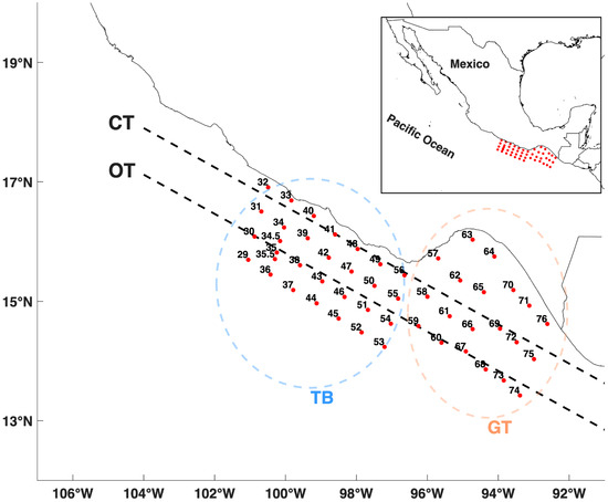
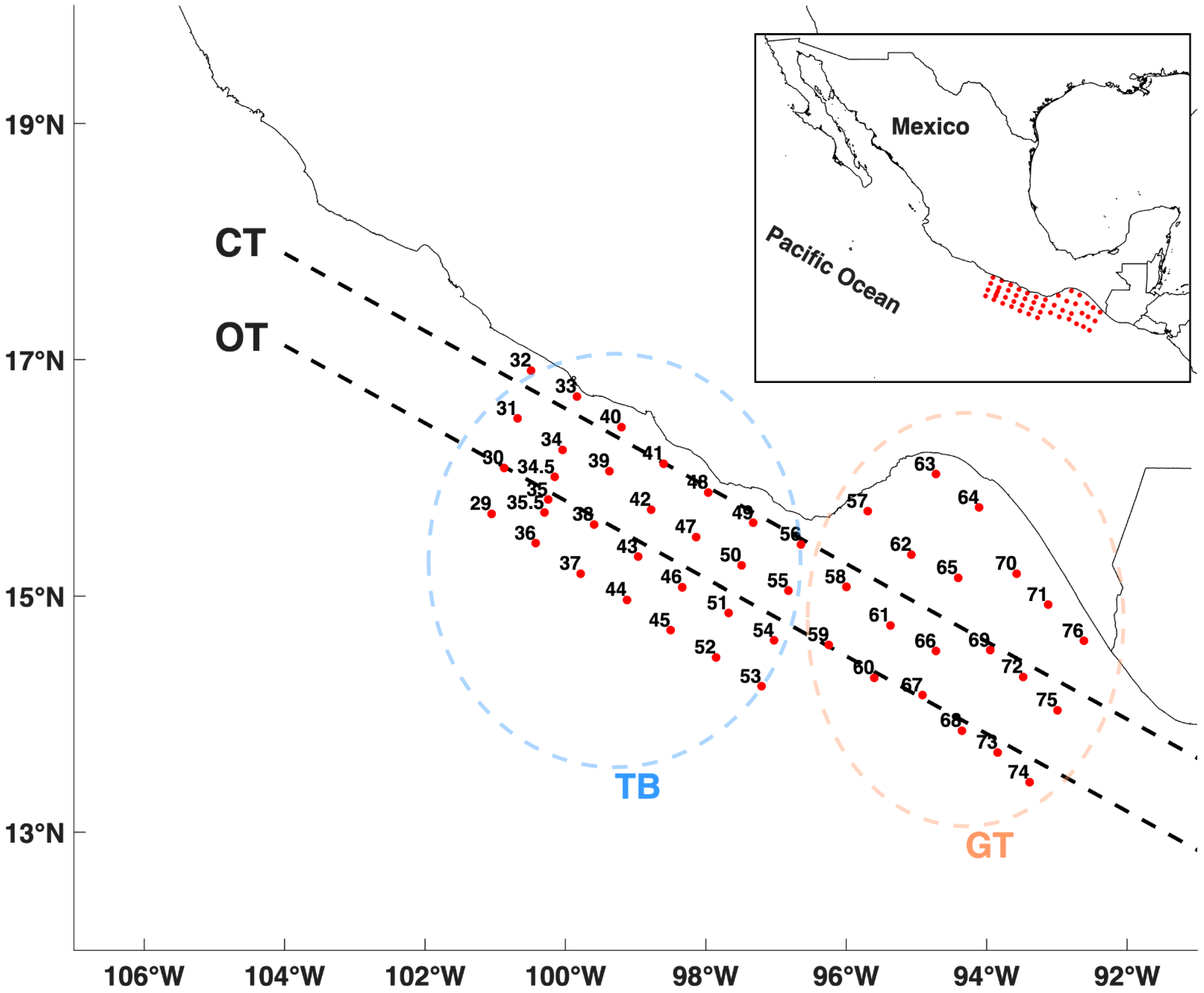
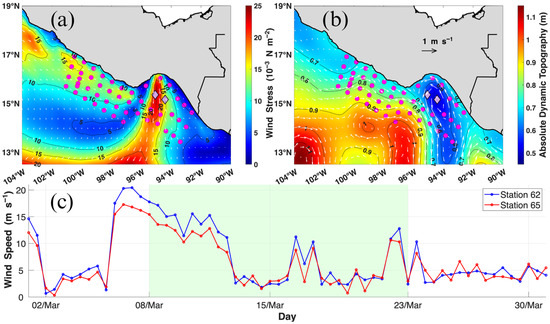
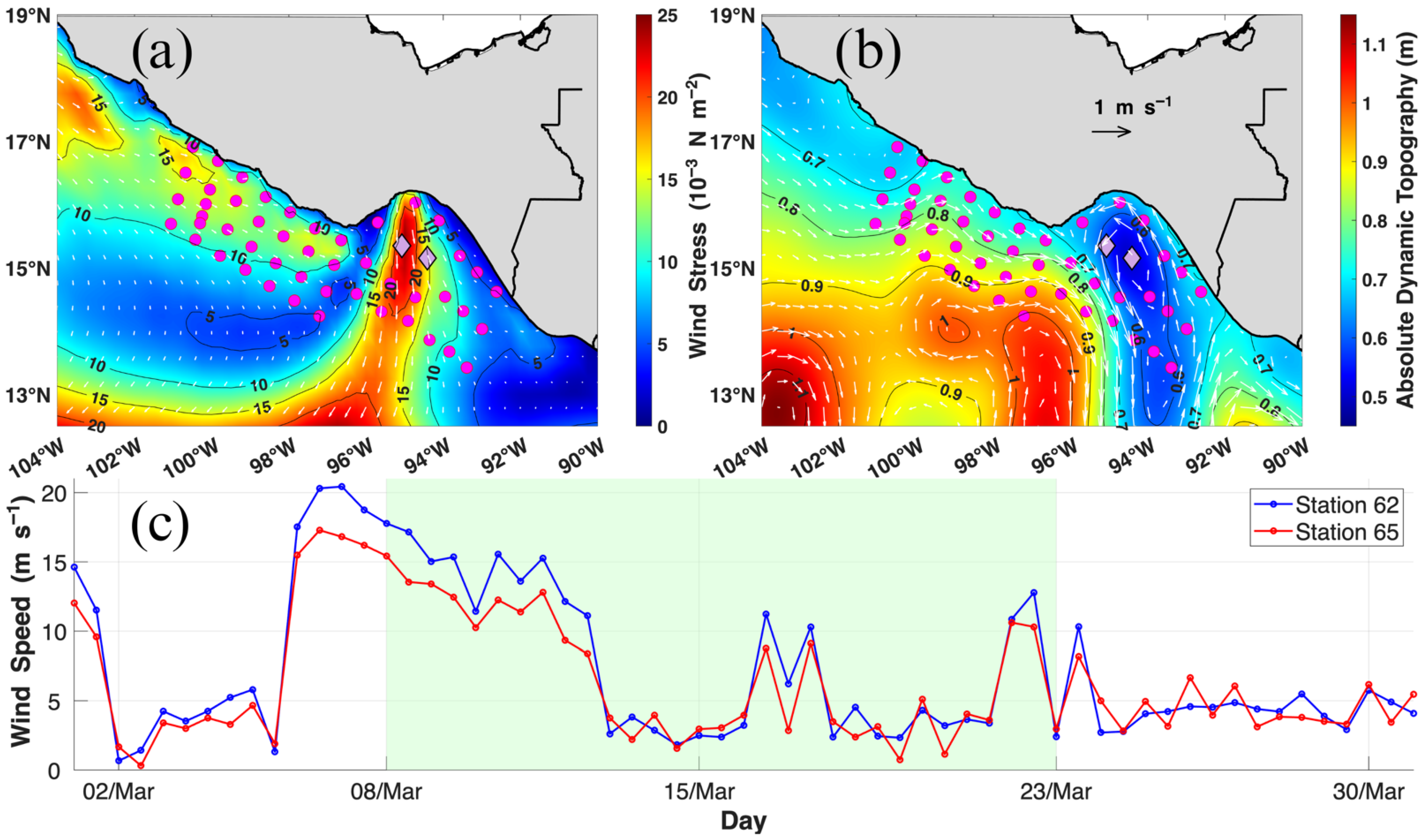
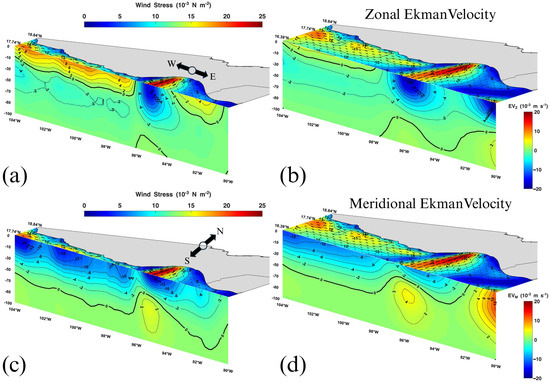
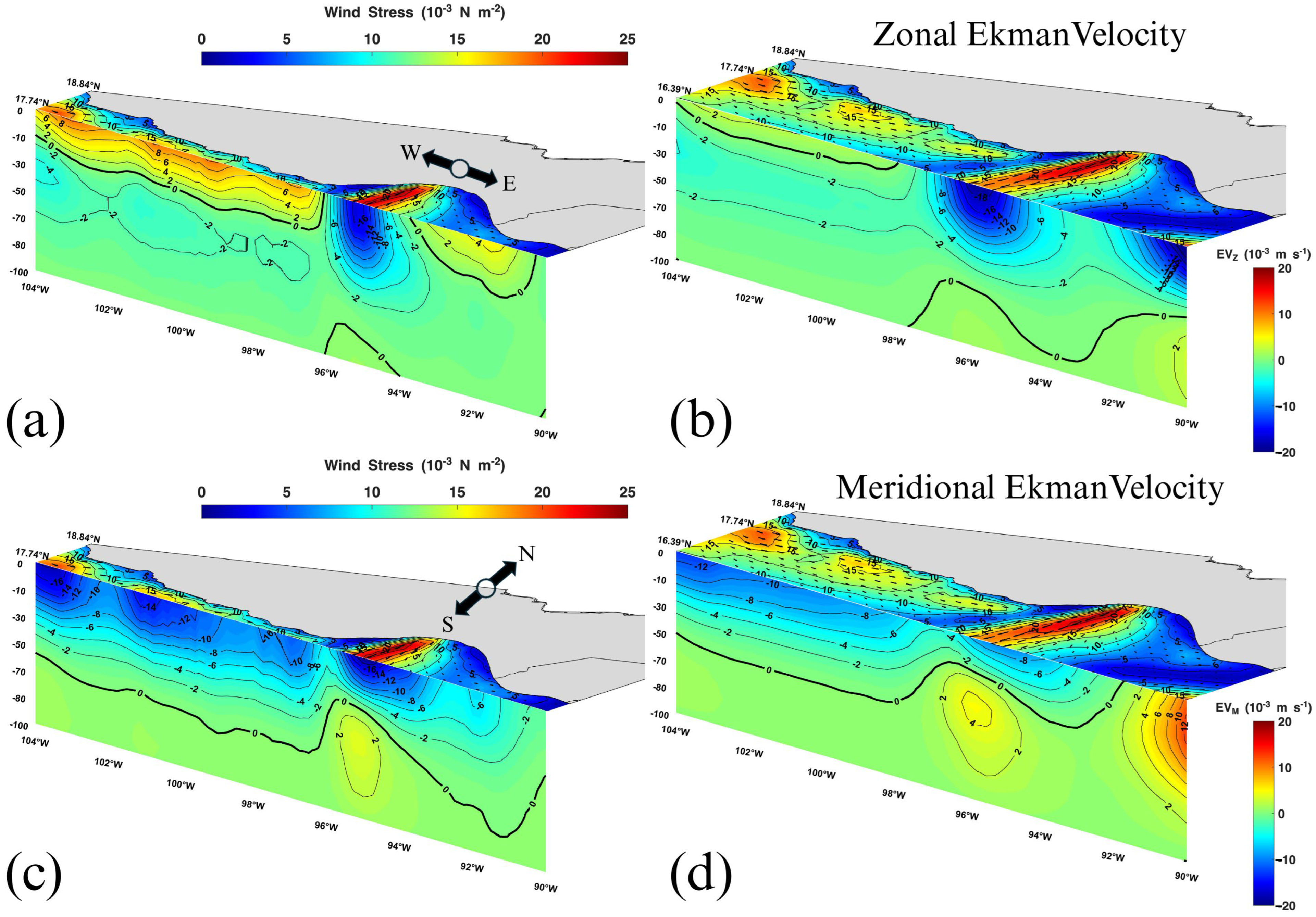
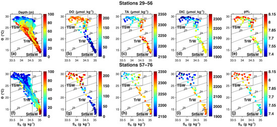
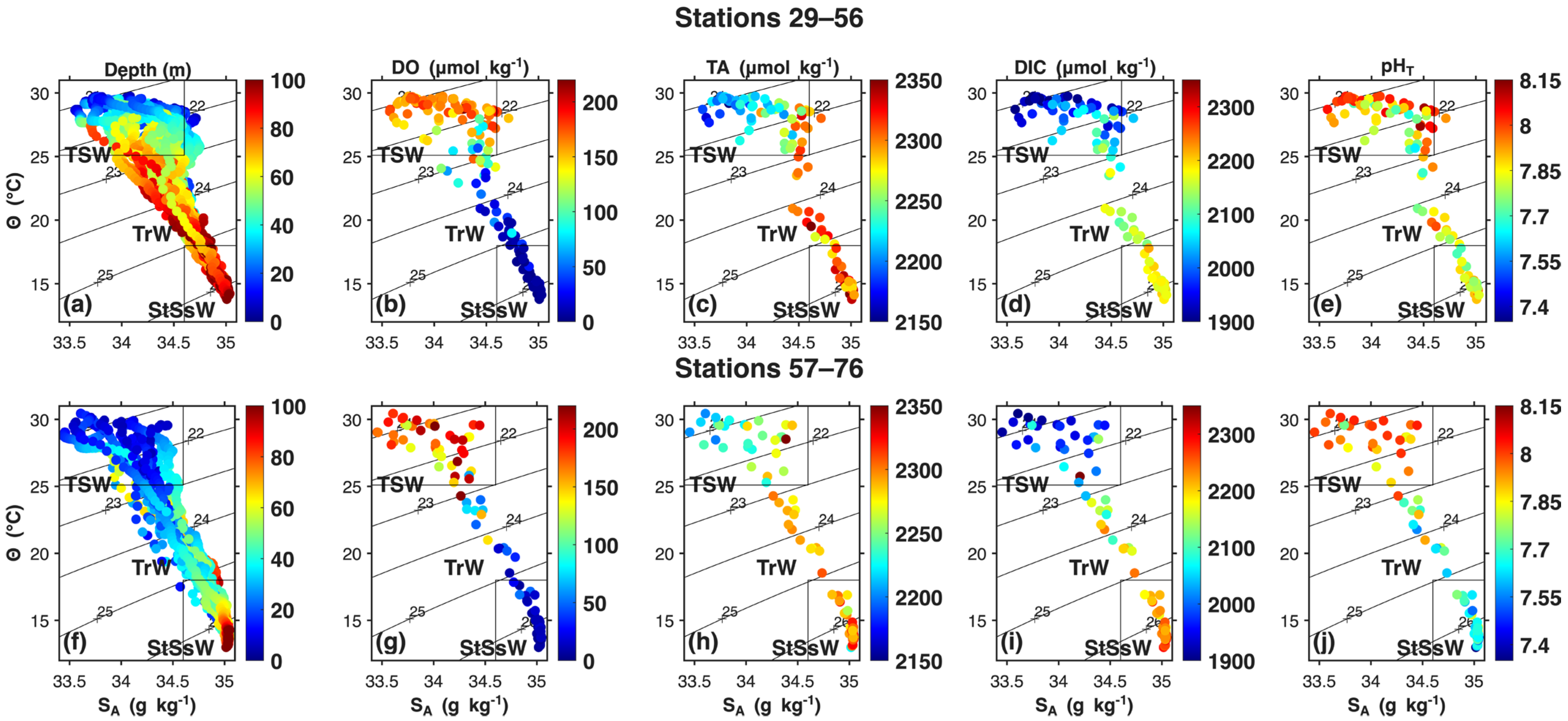
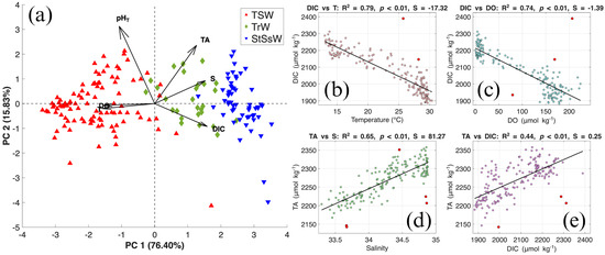
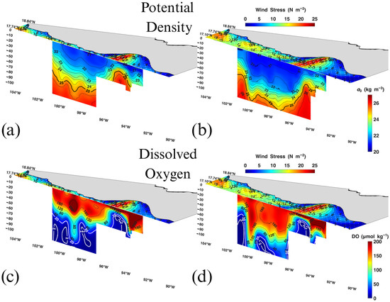
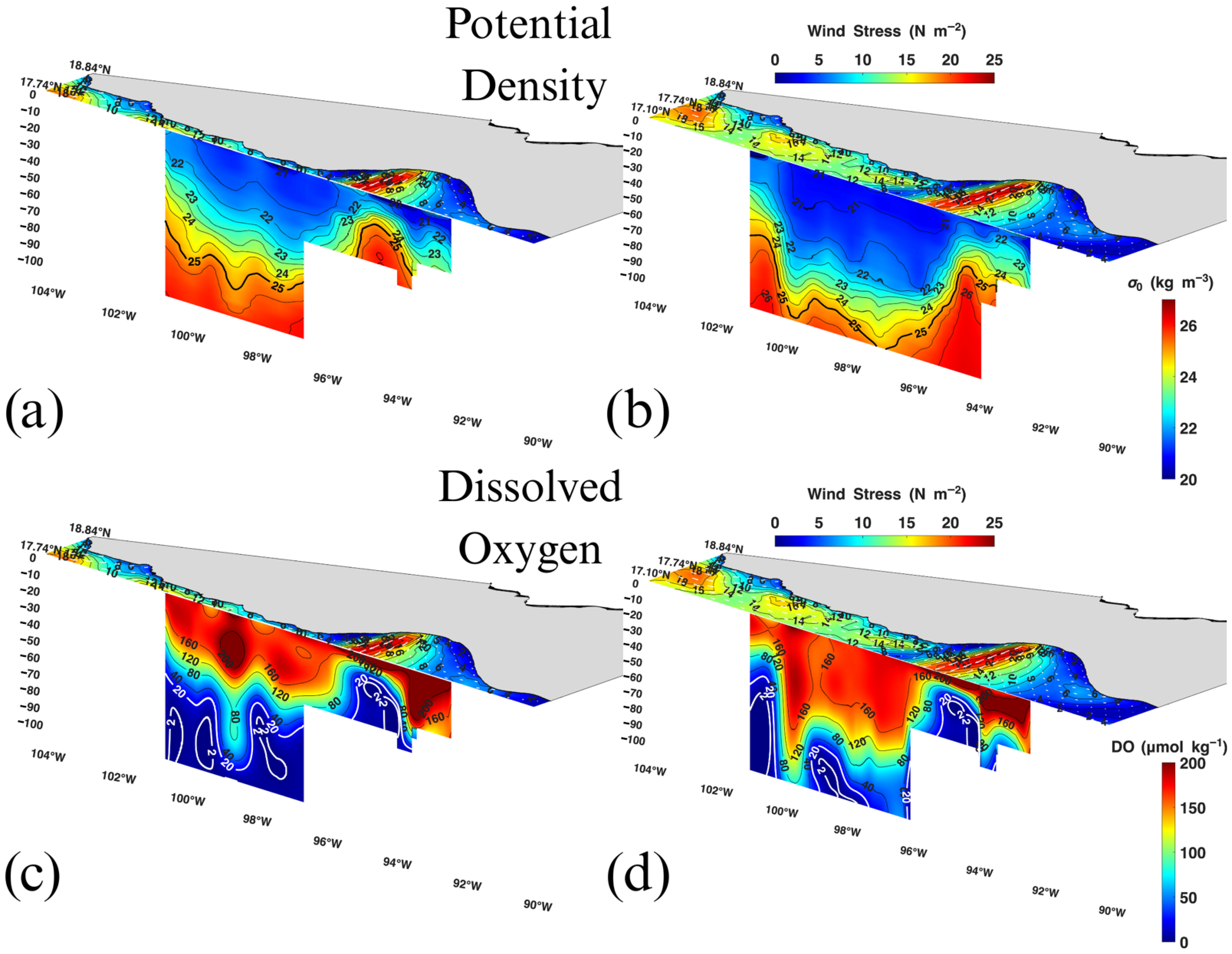
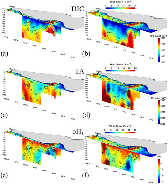
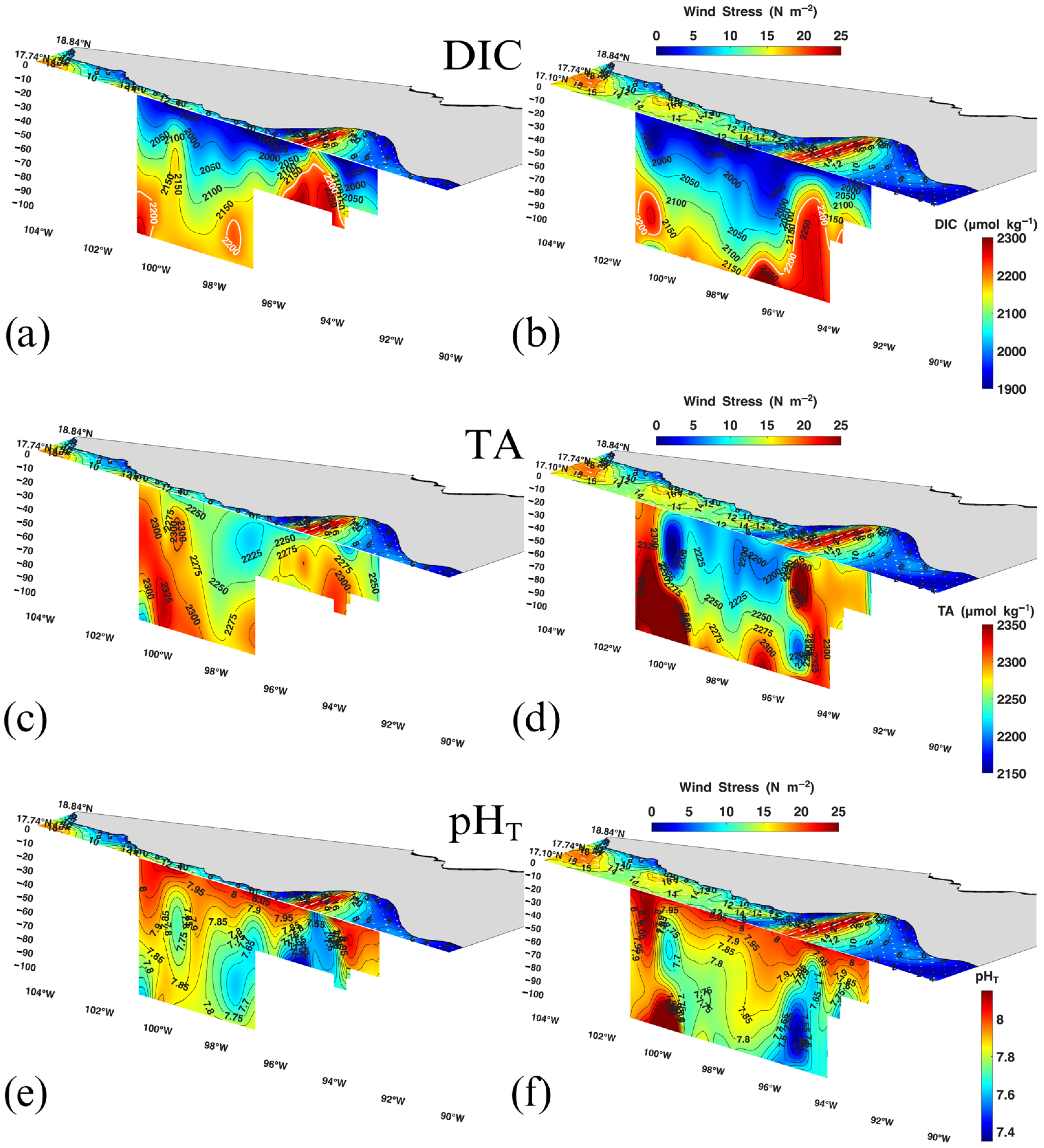
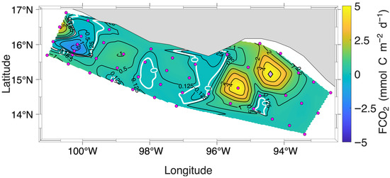
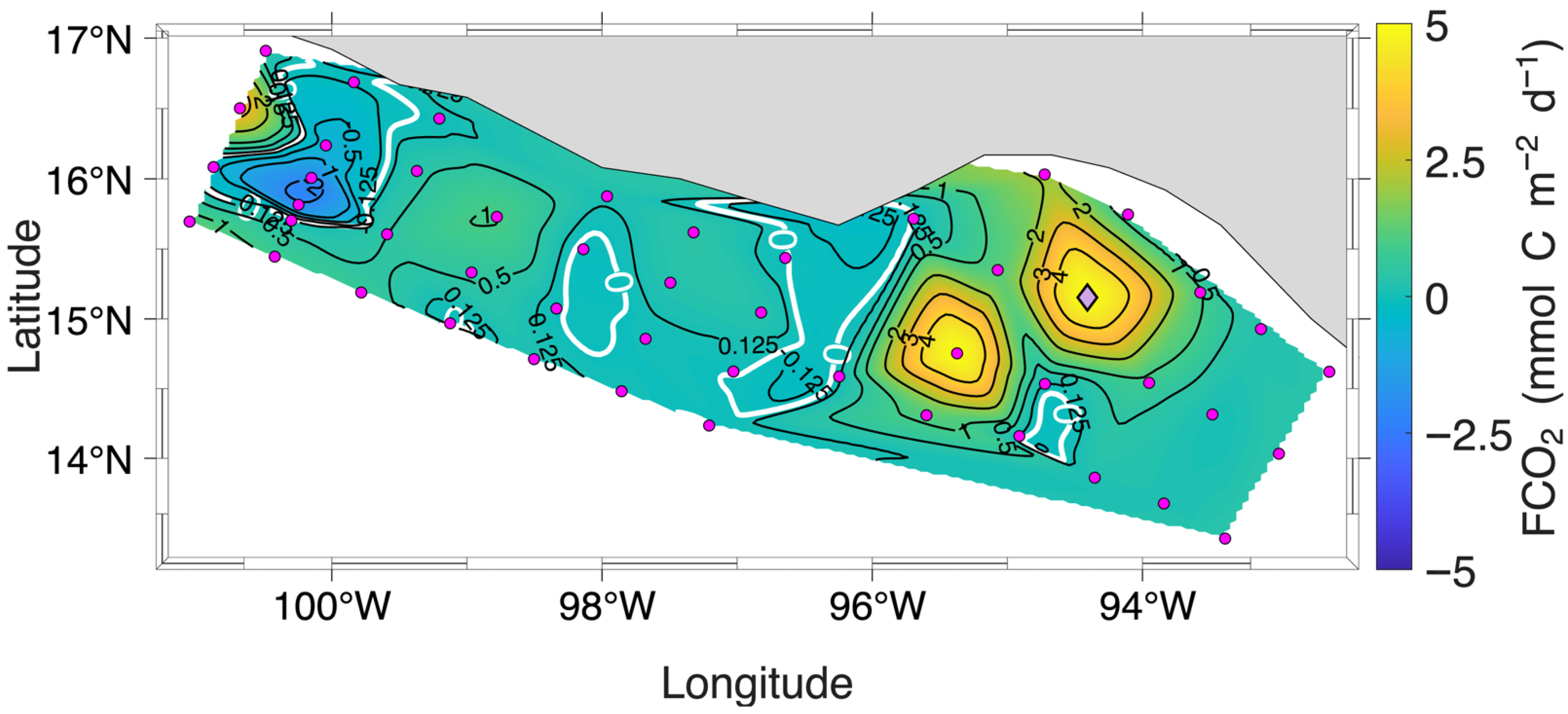
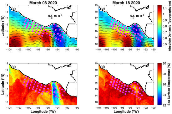
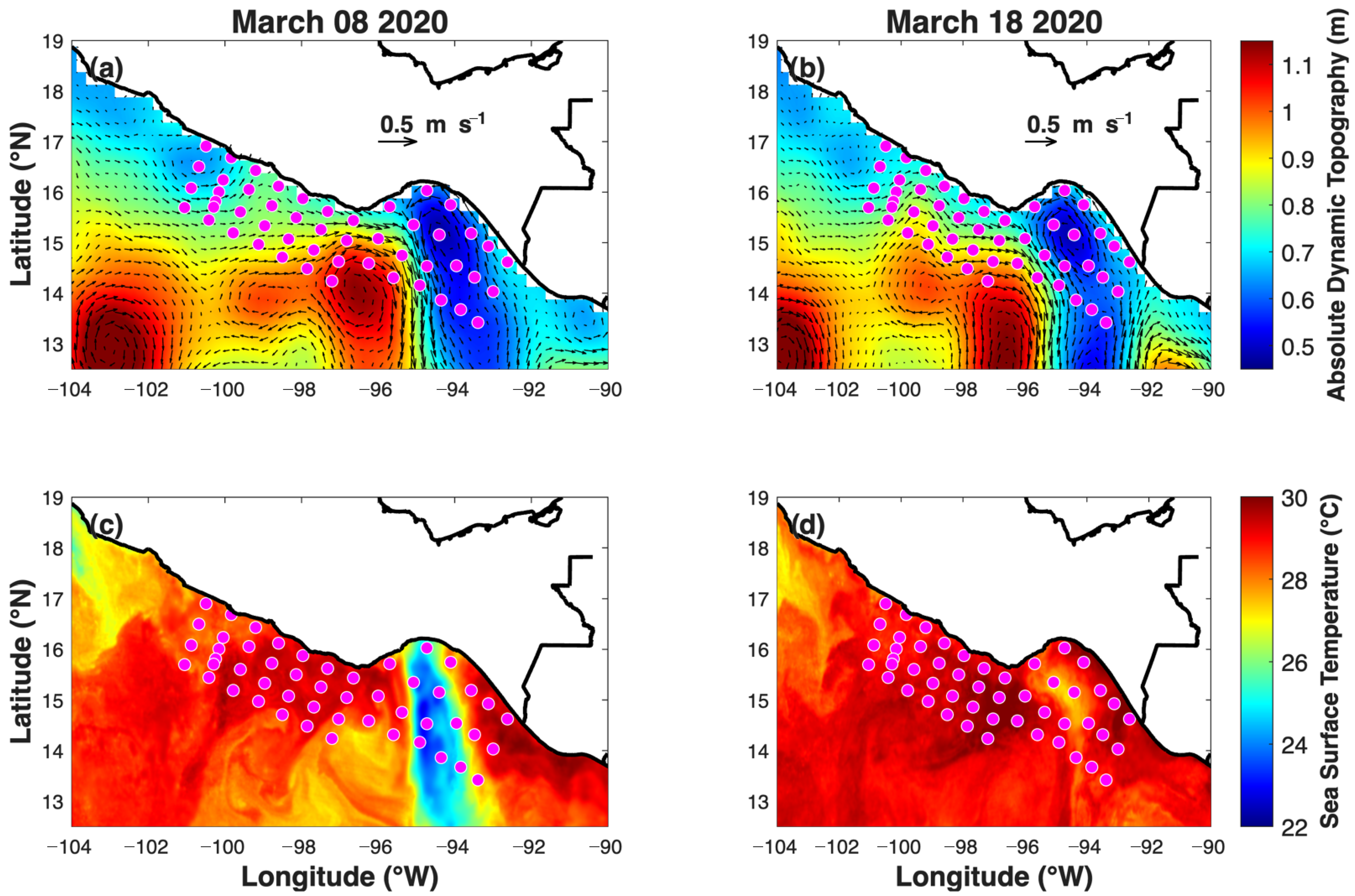

Disclaimer/Publisher’s Note: The statements, opinions and data contained in all publications are solely those of the individual author(s) and contributor(s) and not of MDPI and/or the editor(s). MDPI and/or the editor(s) disclaim responsibility for any injury to people or property resulting from any ideas, methods, instructions or products referred to in the content. |
© 2026 by the authors. Licensee MDPI, Basel, Switzerland. This article is an open access article distributed under the terms and conditions of the Creative Commons Attribution (CC BY) license.