Spatiotemporal Characteristics and Dynamical Analysis of Surface Residual Currents in the Southwestern Taiwan Strait Under Low Wind Condition

Abstract

The residual current is the ocean current after the tidal component has been removed. Understanding the spatiotemporal distribution characteristics of sea surface residual currents is key to revealing the local current field evolution and typical physical oceanographic processes. The Taiwan Strait is in the East Asian monsoon region, where residual currents are significantly influenced by monsoons during periods of high wind speeds. However, the characteristics and dynamic mechanisms of residual currents under low wind speed conditions (≤5 m/s) remain unclear. Based on high-frequency surface wave radar current data and wind field reanalysis data, this study analyzed the characteristics of residual currents in the southwestern Taiwan Strait under low wind speed conditions, focusing on two orthogonal directions: cross-shore and along-shore. During these periods, residual currents exhibit counter-wind current characteristics. These currents cross the Taiwan Bank and generate wave signals with wavelengths ranging from 35.6 km to 65.8 km and durations of 6 to 12 h in the Xiapeng Depression area. These fluctuations are triggered by the combined timing of low winds and nonlinear current–topography interactions. In terms of dynamic mechanisms, the Coriolis force term and the acceleration term dominate the momentum equations in both two orthogonal directions, indicating that the current field is in a non-steady inertial adjustment phase during this period. Furthermore, this study constructs a two-layer ocean model of rotationally modified gravity waves to analyze the influences of topography, oceanic stratification, and steady current velocity on the characteristics of residual current fluctuations under low wind speed conditions. The theoretical model yields spatial scales that closely match the observed wavelength characteristics.

1. Introduction

Sea surface residual current refers to the remaining component of the total sea surface current after removing the tidal current [1]. It is a key factor influencing marine material transport and air–sea interactions [2]. As a strategic waterway connecting the East China Sea and the South China Sea, the Taiwan Strait has garnered significant attention from international researchers. The circulation structure in the strait is strongly modulated by the East Asian monsoon, which features prevailing northeasterly winds in winter and southwesterly or southerly winds in summer [3]. Investigating the dynamics of residual currents in this region holds important implications for marine trade, military activities, and scientific research.

Since the 1980s, advancements in ocean observation technologies and the development of numerical models have gradually revealed the characteristics and influencing factors of residual currents in the Taiwan Strait [4]. Among these factors, wind is a key driver affecting the features of sea surface residual currents in this region [5]. Due to the strong correlation between residual currents and wind fields in the Taiwan Strait, it is generally accepted that the surface residual current is primarily driven by wind stress [6]. A study by Wang (1991) demonstrated that the correlation coefficient between surface residual current velocity and wind speed exceeded the value required by 5% confidence, while the correlation coefficient between current direction and wind direction reached as high as 0.928, indicating statistically significant results [7]. Jan et al. (2002) proposed that there are perennial southward residual currents along the mainland coast and northward residual currents along the western coast of Taiwan, which collectively form the circulation pattern of the Taiwan Strait [8]. However, these understandings are largely based on conditions of moderate to high wind speeds, and the spatiotemporal characteristics and dynamic mechanisms of residual currents during the winter monsoon relaxation period in the Taiwan Strait, when surface wind speeds drop below 5 m/s, have not yet been thoroughly investigated.

Under low wind speed conditions, the response of residual currents to wind forcing exhibits a hysteresis effect [9], during which non-wind-driven dynamic factors (e.g., swell, wave–current interactions, current–topography interactions) dominate the current field. Previous studies have demonstrated that residual currents in the Taiwan Strait are influenced not only by wind fields but also by a combination of multiple factors. For instance, Jiang et al. (2013) and Liao et al. (2018), utilizing the ROMS model and buoy array data, analyzed the 2008 cold disaster event in the Taiwan Strait and highlighted the critical roles of wind field variations, sea level differences, and topographic steering [10,11]. Based on satellite data, Shen et al. (2019), Oey et al. (2014), and Li et al. (2017) explained the formation mechanisms of the winter cross-strait current and the counter-wind current in the Taiwan Strait under low wind speed conditions from the perspective of an imbalance between wind stress and the pressure gradient force [12,13,14]. However, most of these studies rely on single-point buoy observations or numerical simulations and lack comprehensive support from extensive, continuous, in situ measurements of ocean currents.

Compared to single-point buoys and satellite remote sensing, High-Frequency Surface Wave Radar (HFSWR, operating at 3–30 MHz) offers the advantages of all-weather and continuous observation, enabling the acquisition of high-resolution sea surface current data within a nearshore range of approximately 200 km [15,16]. This capability provides a valuable opportunity to analyze the spatiotemporal characteristics of surface residual currents under low wind speed conditions [17,18]. Using HFSWR data from 2005 to 2007, Zhu (2008) analyzed interannual and seasonal variations in the southwestern Taiwan Strait and concluded that surface residual currents are primarily induced by monsoons [19]. Shen (2014) and Lai (2018) also confirmed a strong correlation between winter monsoon winds and residual currents at specific locations [20,21]. However, the dataset used by Shen only covered three days, making it difficult to capture long-term evolutionary features, while Lai’s observational scope did not fully cover the Taiwan Bank topography, limiting a comprehensive investigation of the seabed’s influence on residual currents. Wen et al. (2021) utilized the correlation between wind and residual currents to develop a method for retrieving wind speed based on wind-induced current [22]. Nevertheless, these studies lacked an in-depth consideration of additional dynamic factors—such as the pressure gradient force, the Coriolis force, and bottom friction stress—during periods of low wind speed.

In contrast to previous studies, this paper sought to elucidate the dynamic characteristics of residual currents during low-wind periods. Integrating HFSWR observations of ocean currents and wind field reanalysis data, this study focused on the spatiotemporal distribution characteristics of surface residual currents in the southwestern Taiwan Strait during low wind speed periods. From the two orthogonal directions of cross-shore and along-shore, it specifically analyzed the generation of counter-wind current and the submesoscale fluctuations excited near the Taiwan Bank. Furthermore, the dynamic mechanisms of the residual currents were investigated, and a theoretical model of rotationally modified gravity waves was constructed to explore the generation mechanism of these fluctuations. This research is expected to provide new theoretical insights into the understanding of ocean dynamic processes in the Taiwan Strait during monsoon relaxation periods.

This paper is structured as follows. Section 1 provides the introduction. Section 2 describes the data and methods used in this study. Section 3 presents the experimental results. Section 4 offers a discussion of the findings, and Section 5 concludes with a summary of the entire paper.

2. Materials and Methods

2.1. Data

2.1.1. HFSWR Ocean Currents

An ocean current observation experiment was conducted in the Taiwan Strait using two High-Frequency Surface Wave Radar systems deployed along the coast of Fujian Province at Dongshan and Longhai. Through long-term comparative testing, the surface vector currents obtained by the radar within the effective detection area showed good agreement with the actual sea surface current field. In high-accuracy zones, the errors in current speed and direction were small, with the minimum Root Mean Square Error (RMSE) values reaching only 7.5 cm/s and 15.5°, respectively. It has been verified that the actual observational accuracy of this radar observation system meets the operational requirements of similar products both domestically and internationally [23].

The current data used in this study were sea surface current fields obtained from the jointly covered area of the dual-station HFSWR. The data covered the period from 29 January 2013 to 26 March 2013, with a radar operating frequency of 8.75 MHz, an output interval of 10 min, and a spatial resolution of 1/40°.

2.1.2. OTIS Tidal Current Data

Tidal current data were sourced from the Oregon State University Tidal Inversion System (OTIS). This system employs an efficient Generalized Inverse (GI) method for barotropic ocean tides, integrating dynamical information with observational data to solve the Shallow Water Equations (SWEs), thereby constructing global and regional tidal models and providing tidal estimation and forecasting solutions. OTIS offers capabilities such as the direct computation of sea surface height, estimation of tidal currents, control of boundary conditions, and generation of covariance realism maps, which contribute to a deeper understanding of ocean tidal processes [24,25].

Using MATLAB relevant mathematical matrix processing software, the model was run to output tidal currents for the Taiwan Strait region based on the TPXO9.0-atlas tidal model (available at: https://www.tpxo.net/global, accessed on 12 July 2025), which includes eight major tidal constituents (M2, S2, O1, K1, N2, K2, P1, Q1). The output results for the Taiwan Strait area had a spatial resolution of 1/30° and a temporal resolution of 10 min.

2.1.3. Wind Field Data

This study utilized wind field data from the ERA5 reanalysis dataset produced by the European Center for Medium-Range Weather Forecasts (ECMWF), combined with in situ observations from the buoy operated by the Fujian Marine Forecasting Observatory. The data covered the period from 29 January 2013 to 26 March 2013.

The ERA5 reanalysis wind field data consisted of single-level hourly records [26], with the $U$ and $V$ component wind fields at a height of 10 m above sea level selected for this study, at a spatial resolution of 0.25°. The buoy wind data comprised a time series of mean surface wind speed and direction at the location (23.46° N, 118.33° E), with a temporal resolution of 30 min.

During winter (December to February), the Taiwan Strait experiences its highest mean wind speeds of the year, with average speeds in its central region typically ranging between 12 m/s and 14 m/s. In contrast, the mean wind speed in the southwestern part of the Taiwan Strait is slightly lower than that in the central strait [27].

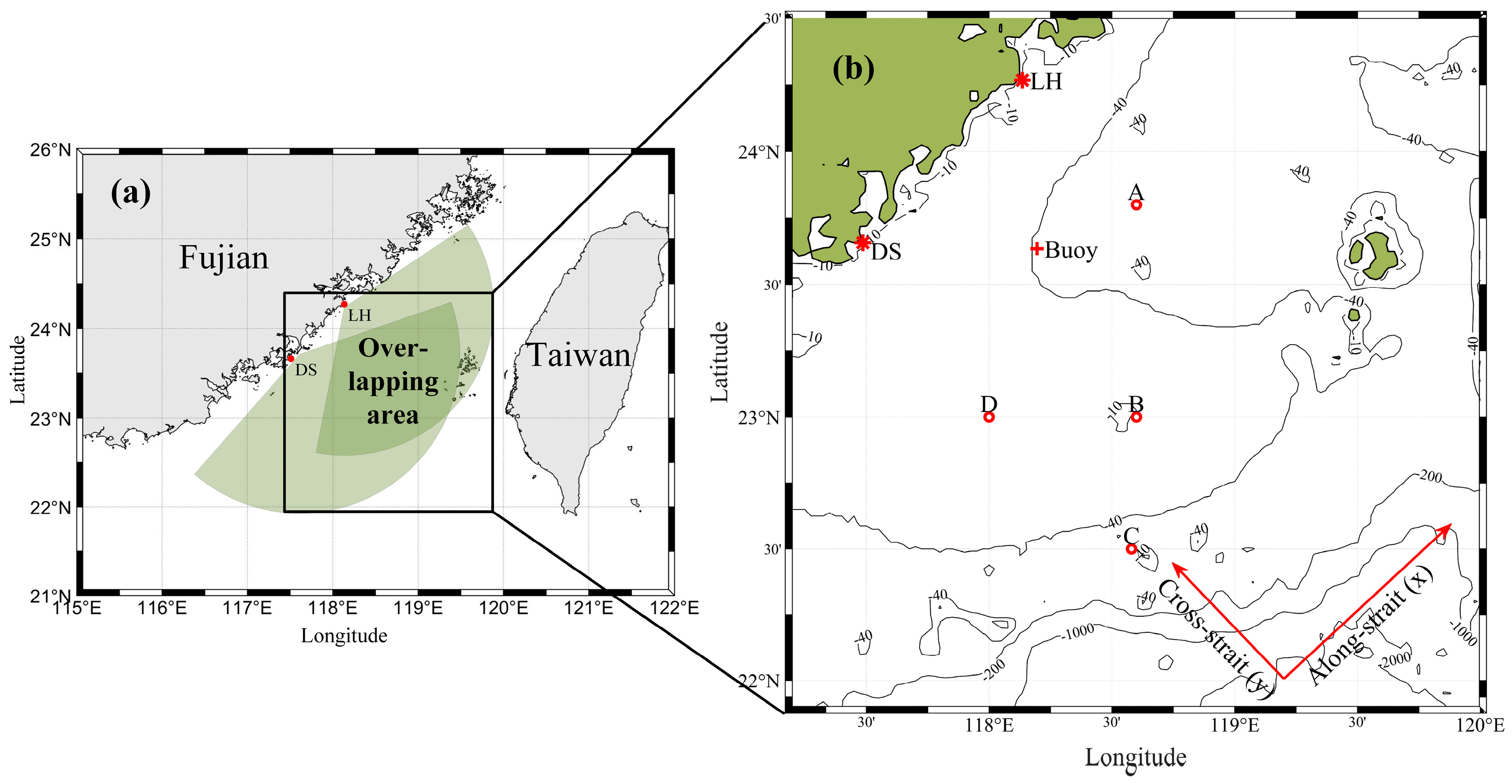
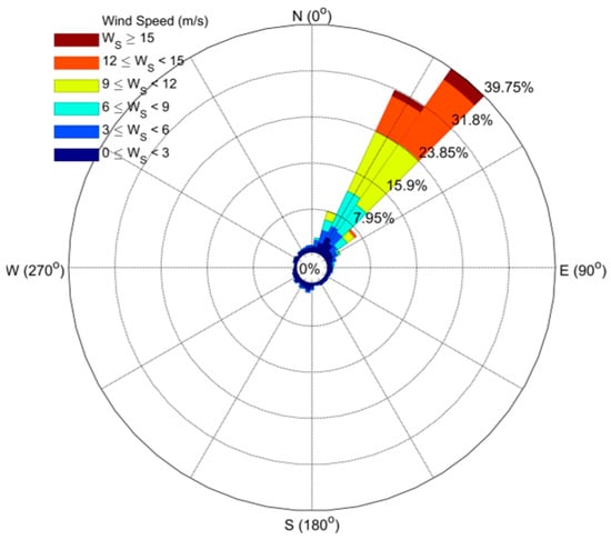
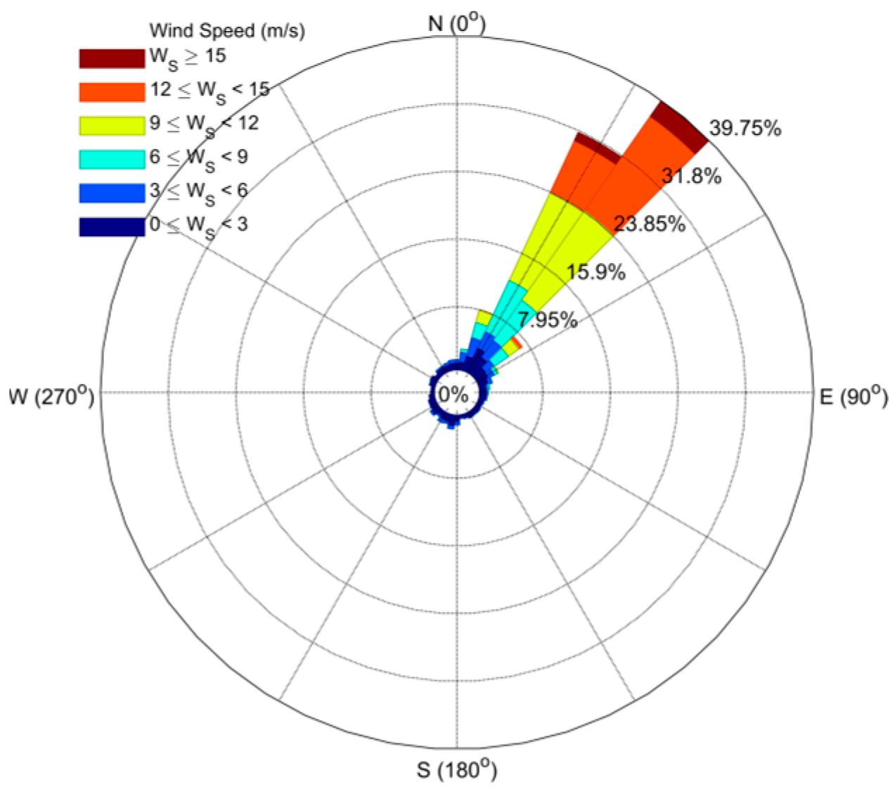
A sea surface wind observation buoy, indicated by the red cross in Figure 1b, recorded the mean wind speed and direction at a 10 m height above sea level during the experiment. The buoy’s measurement range covers wind speeds from 0.5 m/s to 60 m/s and directions from 0° to 360°, with a specified error of 5% for speed and 10° for direction. As shown in the wind rose diagram (Figure 2), northeasterly monsoons prevailed during the experiment, with wind speeds ranging from 0 to 16 m/s. The dominant wind directions were concentrated at 30° and 42.5° (where 0° represents true north) within the northeastern sector. In terms of occurrence frequency, these two directional bins collectively accounted for more than 71.5% of the recorded data.

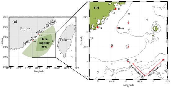
Figure 1. Joint Coverage Area: (a) shows the spatial extent of the jointly covered region. In panel (b), red asterisks represent radar sites, LH represents Longhai Station, DS denotes Dongshan Station, red crosses indicate buoy positions, labels A, B, C, and D mark the four selected points, the x-axis denotes the alongshore direction, and the y-axis represents the cross-shore direction. Adapted with permission from [28]. 2024 X. Peng.

Figure 2. Wind Rose.

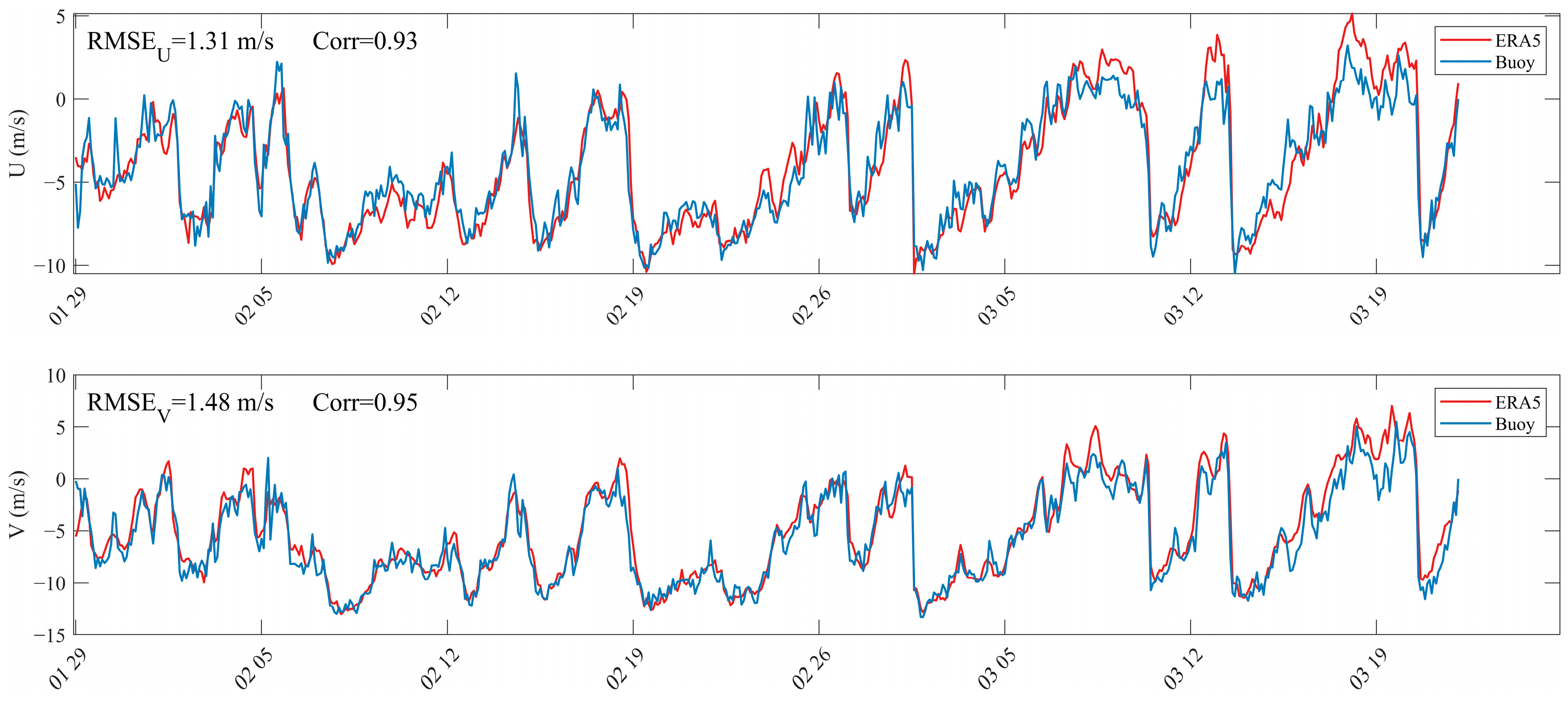
To evaluate the applicability of the ERA5 wind field data within the radar observation area, the RMSE and correlation coefficient between the ERA5 wind data at the buoy location and the buoy wind data were calculated, as shown in Figure 3.

Figure 3. Comparison between the buoy-measured wind speeds and ERA5 wind speeds at the buoy locations, the x-axis represents the period from 29 January 2013 to 26 March 2013.

The results showed RMSE values and correlation coefficients of 1.31 m/s ($U$ component), 0.93, 1.48 m/s ($V$ component), and 0.95, respectively. This indicates that the ERA5 wind field data are highly reliable. To further compare the spatial distribution characteristics of the wind field and residual currents, the ERA5 data were subsequently used to represent the local wind field.

2.2. Methods

2.2.1. Quality Control of Vector Current

The current data used in this study were vector currents from the jointly covered area of the two radar systems. To obtain current field results with high reliability, quality control was applied both spatially and temporally.

First, spatial outliers were identified and removed. The complete spatial current field at each time step was examined, and values that deviated significantly from the temporal mean of the current field at that time were eliminated.

$$|v_t(x,y)-{\overline{v}}_t|>2v_{std}$$

(1)

In Equation (1), $v_t(x,y)$ represents the current velocity at any spatial point at time $t$, $\overline{v_t}$ denotes the mean current velocity of the current field at time $t$, and $v_{std}$ is the standard deviation of the current velocities across all spatial points in the field at time $t$. This method eliminates values that differ from the mean current velocity by more than two standard deviations.

Second, temporal outliers were removed. The time series at each spatial point was examined, and values that deviated significantly from the mean of the time series at that location were eliminated. This method removes values that differ from the temporal mean current velocity by more than two standard deviations.

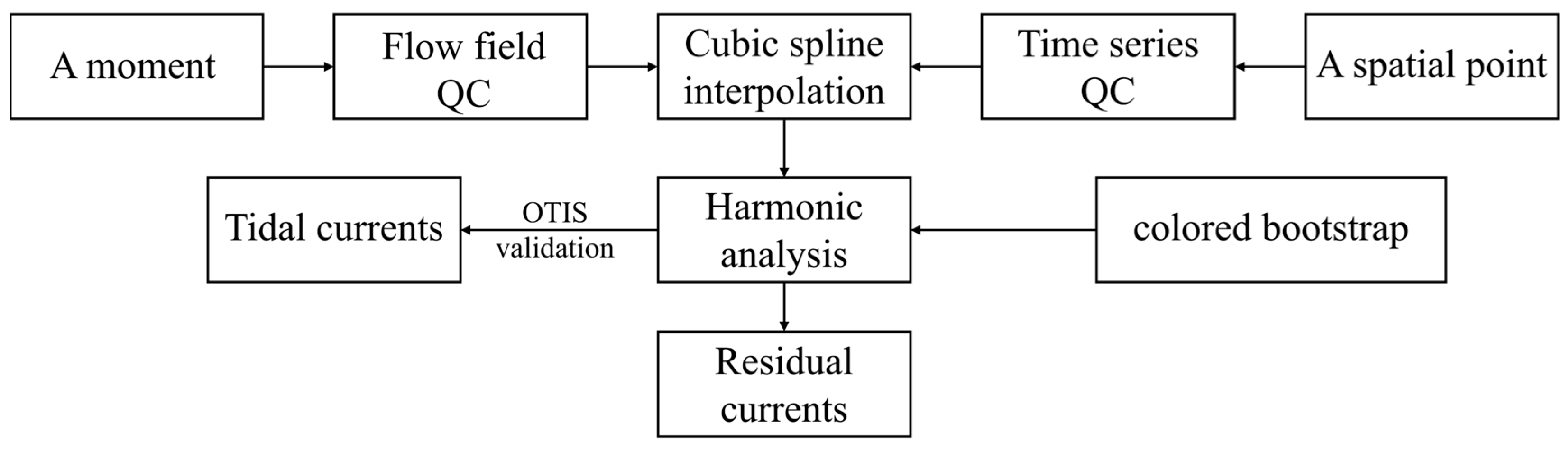
Third, temporal gaps were filled using a cubic spline interpolation function. Spatial areas with a data sampling rate exceeding 70% were then selected for subsequent analysis. It was verified that within this region, the Geometric Dilution of Precision (GDOP) value at each point was below 2.5.

2.2.2. Harmonic Analysis and Validation

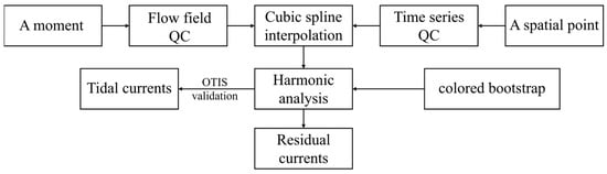
To obtain high-accuracy residual currents, accurate separation of the tidal components is first required (as shown in Figure 4). In this study, harmonic analysis was performed on each spatial point within the vector current field. The uncertainty parameters were configured based on a colored bootstrap method under an uncorrelated bivariate colored noise model. This approach not only captures the attenuation characteristics of the background energy spectrum in the high-frequency band but also adapts to the non-Gaussian distribution of errors under low signal-to-noise ratio conditions [29].

Figure 4. Quality control (QC) and harmonic analysis validation.

To further validate the accuracy of the tidal currents extracted via harmonic analysis, relevant mathematical matrix processing software was used to run the OTIS model and output tidal constituents based on the TPXO9.0-atlas tidal model. The comparison was focused on the four dominant constituents: M2, S2, O1, and K1. The spatial resolution of the OTIS output in the Taiwan Strait area was 1/30°, while that of the High-Frequency Surface Wave Radar (HFSWR) currents was 1/40°. Due to this difference in spatial resolution, the comparison process involved determining the radar-derived tidal current value at a given point and then matching it with the nearest model-derived tidal current value, with the maximum allowable distance for this matching not exceeding 5 km.

2.2.3. Spatiotemporal Resolution Alignment

Distance Weighted Interpolation is a widely used spatial interpolation method, often applied to estimate values at unknown locations based on known data points. Grounded in the basic assumption that “closer distances imply greater influence or contribution to the target point”, its core idea is to use the reciprocal of the distance between known and unknown points as a weight, performing a weighted average of the known values to estimate the value at the target location [30]. Among these methods, the most classic is Inverse Distance Weighting (IDW), which has been extensively applied in fields such as Geographic Information Systems, environmental science, and meteorology [31].

The ERA5 reanalysis wind field data are uniformly distributed spatially and contain many interpolation points. After repeated application of Inverse Distance Weighting interpolation, high data smoothness and fidelity are ensured. Following gap-filling in the spatial domain using this interpolation method, the wind field achieves a spatial resolution of 0.025°.

Cubic Spline Interpolation, a high-order interpolation method, constructs a smooth curve using piecewise cubic polynomials. It not only maintains high accuracy in results but also ensures continuity of the second-order derivative across the entire domain. This method is widely applied in numerous fields, including atmospheric sciences, numerical analysis, and signal processing. Cubic Spline Interpolation was chosen for this study due to its optimal balance between accuracy, smoothness, and numerical stability. Unlike linear interpolation, which produces unsmooth piecewise linear fits, or high-order global polynomial interpolation, which is prone to oscillatory Runge‘s phenomenon [32], the piecewise cubic polynomial approach of splines ensures C² continuity (smooth curvature) while maintaining robustness against overshooting [33]. The requirement for a smooth temporal evolution of wind fields and residual currents aligns perfectly with the C² continuity guarantee of cubic splines. This smoothness is crucial for subsequent dynamic analysis or derivative-based calculations [34].

Cubic Spline Interpolation was applied temporally to fill gaps in the time series of both the ERA5 reanalysis wind field data and the single-point measurements from the buoy. After pre-processing, the wind field data achieved a temporal resolution of 10 min. Additionally, both wind datasets were temporally aligned with the residual current data to ensure consistent time coverage.

3. Results

3.1. Spatiotemporal Patterns of Low-Wind Residual Currents

A statistical analysis was performed on the reanalysis wind field data and buoy wind data used in this study, categorizing wind speeds in the Taiwan Strait into three intervals: 0–5 m/s as low wind speed, 5 m/s–10 m/s as moderate wind speed, and greater than 10 m/s as high wind speed [35,36]. The residual currents, after tidal removal, were further smoothed by filtering out high-frequency components, and the resulting data were used for subsequent correlation analysis.

To investigate the triggering mechanism of surface residual current fluctuations under low wind speed conditions, statistics were compiled on the number of triggering events, their spatial extent, and the duration of individual events. The temporal correlation between the wind field and surface residual currents in the along-shore direction was also analyzed. This study employed the method proposed by Kundu (1976) for calculating the correlation coefficient between two sets of vector time series [37]:

$$\rho ={\displaystyle \frac{U_c^{\ast }{U}_w}{\sqrt{U_c^{\ast }{U}_c}\sqrt{U_w^{\ast }{U}_w}}}$$

(2)

In Equation (2), $U_c$ and $U_w$ denote the residual current vector and wind vector, respectively, and the asterisk $\ast$ represents the complex conjugate. The resulting value $\rho$ is a complex number: its magnitude represents the correlation coefficient, and its phase denotes the mean deflection angle.

3.1.1. Correlation Analysis

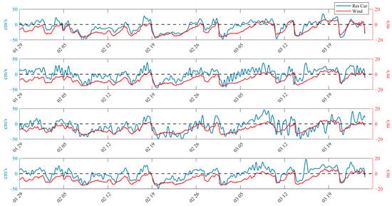
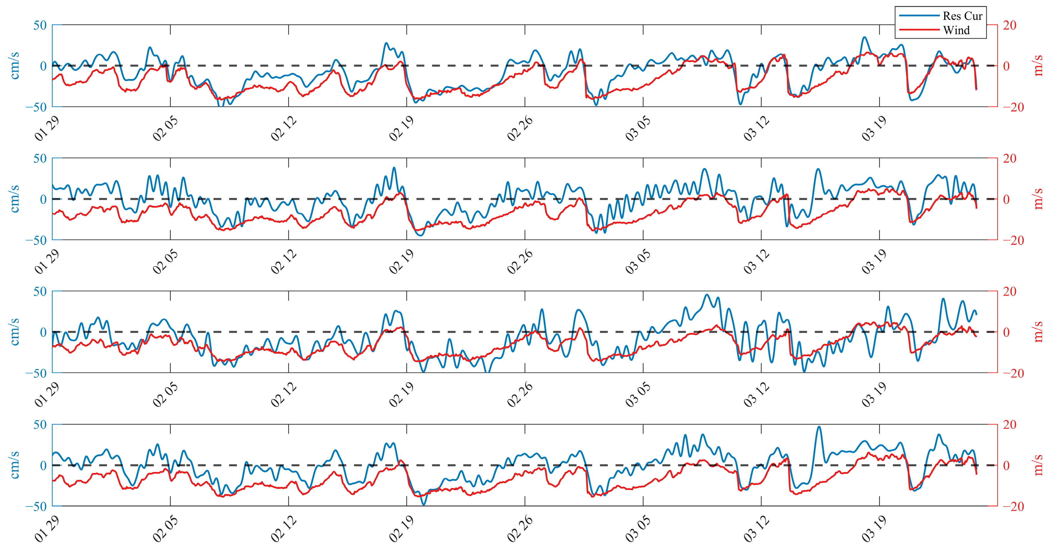
This study utilized residual current data and the ERA5 dataset to quantitatively analyze the influence of the prevailing northeasterly monsoon in winter on the spatiotemporal distribution characteristics of residual currents in the southwestern Taiwan Strait. Figure 5 presents a comparative analysis of the time series of residual currents and wind speeds at four selected locations (A, B, C, and D), where both the wind field and residual currents were projected onto the along-shore direction (with northeast defined as the positive $x$ axis).

Figure 5. Comparison of wind and residual currents in the along-shore direction at locations A to D (from top to bottom), the x-axis represents the period from 29 January 2013 to 26 March 2013. Reproduced from [38].

As clearly shown in Figure 5, the local wind field and residual currents exhibited significant correlation, with correlation coefficients in the $x$ axis direction all above 0.9. Throughout the experiment period (especially from 7 February to 24 March), the winter monsoon displayed quasi-periodic burst characteristics, with an average interval of about 10 days. Cold air masses, accompanied by leading cold fronts, swept across the study area. After each burst phase, conditions rapidly transitioned into a prolonged relaxation period, during which wind strength gradually weakened, and direction occasionally shifted, until the arrival of the next cold front. From the time series, it is evident that residual currents respond rapidly during monsoon bursts, with velocity sharply increasing and peaks reaching up to 50 cm/s. Following a burst, the speed of the residual current gradually decreases, and its direction may even reverse. For example, during sustained southwesterly winds, the residual current shifts to a northeastward direction, forming a typical counter-wind current (CWC), which represents a transitional current pattern. Instances of this counter-wind current were observed at Point A on 18 February, 27 February, and 9 March.

To further quantify the correlation between the residual current vector and the wind vector, this study applied the method for calculating the correlation coefficient of vector time series proposed by Kundu. The results show that during the experiment period, at the buoy location, the correlation coefficient between the residual current vector and the ERA5 wind vector was 0.66, with a deflection angle of 1.78°. Similarly, the correlation coefficient between the residual current vector and the buoy wind vector was 0.65, with a deflection angle of 8.16°. In the actual marine environment, factors such as variable turbulent viscosity and Stokes drift, combined with the interaction between the prevailing northeasterly monsoon in winter and the relatively shallow bathymetry of the Taiwan Strait, objectively account for the differences observed above.

3.1.2. Residual Current Fluctuations

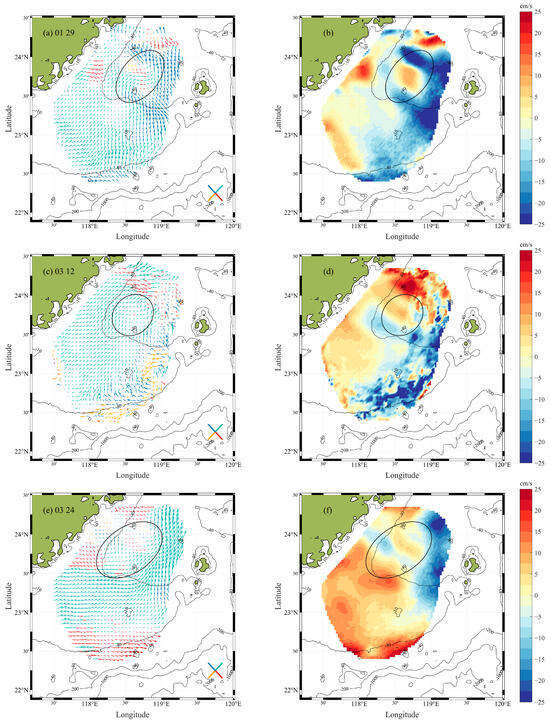
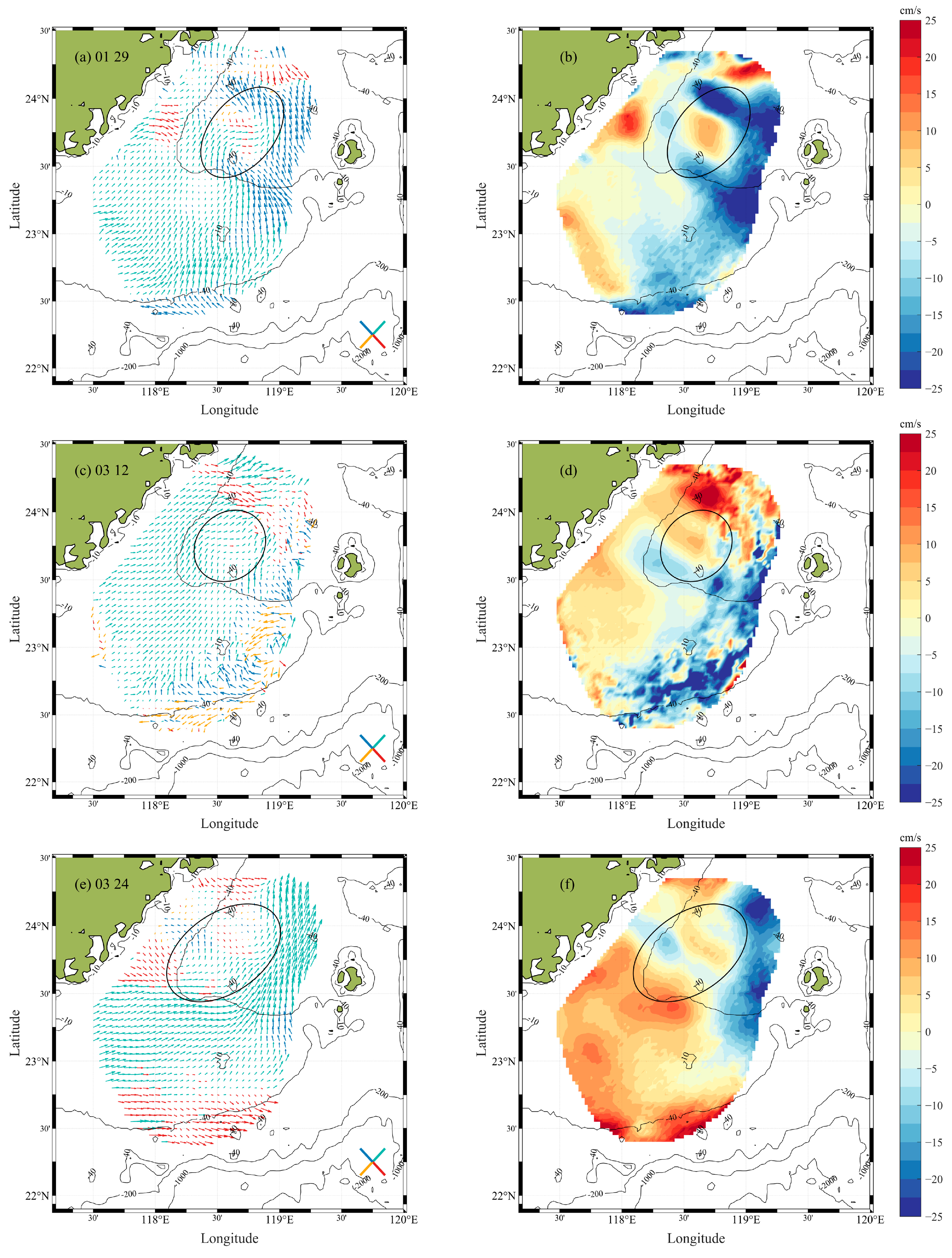
Based on the findings presented in Section 3.1.1, the monsoon relaxation period was identified as a key triggering condition for the formation of the counter-wind current. During this phase, the residual currents exhibit a northeastward direction, opposite to the prevailing northeasterly monsoon. In this study, submesoscale fluctuations in the residual currents were observed in the Xiapeng Depression area north of the Taiwan Bank (as marked in Figure 6), with each event lasting no more than 12 h.

Figure 6. Wave characteristic cases: Case 1 on 29 January (a,b); Case 2 on 12 March (c,d); Case 3 on 24 March (e,f). Left panels (a,c,e) show the current patterns highlighting the current direction; right panels (b,d,f) display the cross-shore component of residual currents, with positive values indicating the southeastward current.

The three cases described corresponded to UTC times 04:00 on 29 January 2013, 18:00 on 12 March, and 06:00 on 24 March, respectively. Taking panels (a) and (b) in Figure 6 as an example: panel (a) illustrates the spatial pattern of the residual currents emphasizing the current direction, where red, blue, cyan, and yellow represent currents oriented approximately southeastward, northwestward, northeastward, and southwestward, respectively. Panel (b) shows the spatial distribution of the cross-shore current, with currents directed southeastward defined as positive. As seen in the figure, the fluctuations were primarily concentrated in the Xiapeng Depression area north of the Taiwan Bank, extending spatially over about one to two wavelengths, with wavelengths ranging from 30 km to 70 km.

3.1.3. Fluctuation Characteristics Analysis

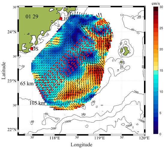
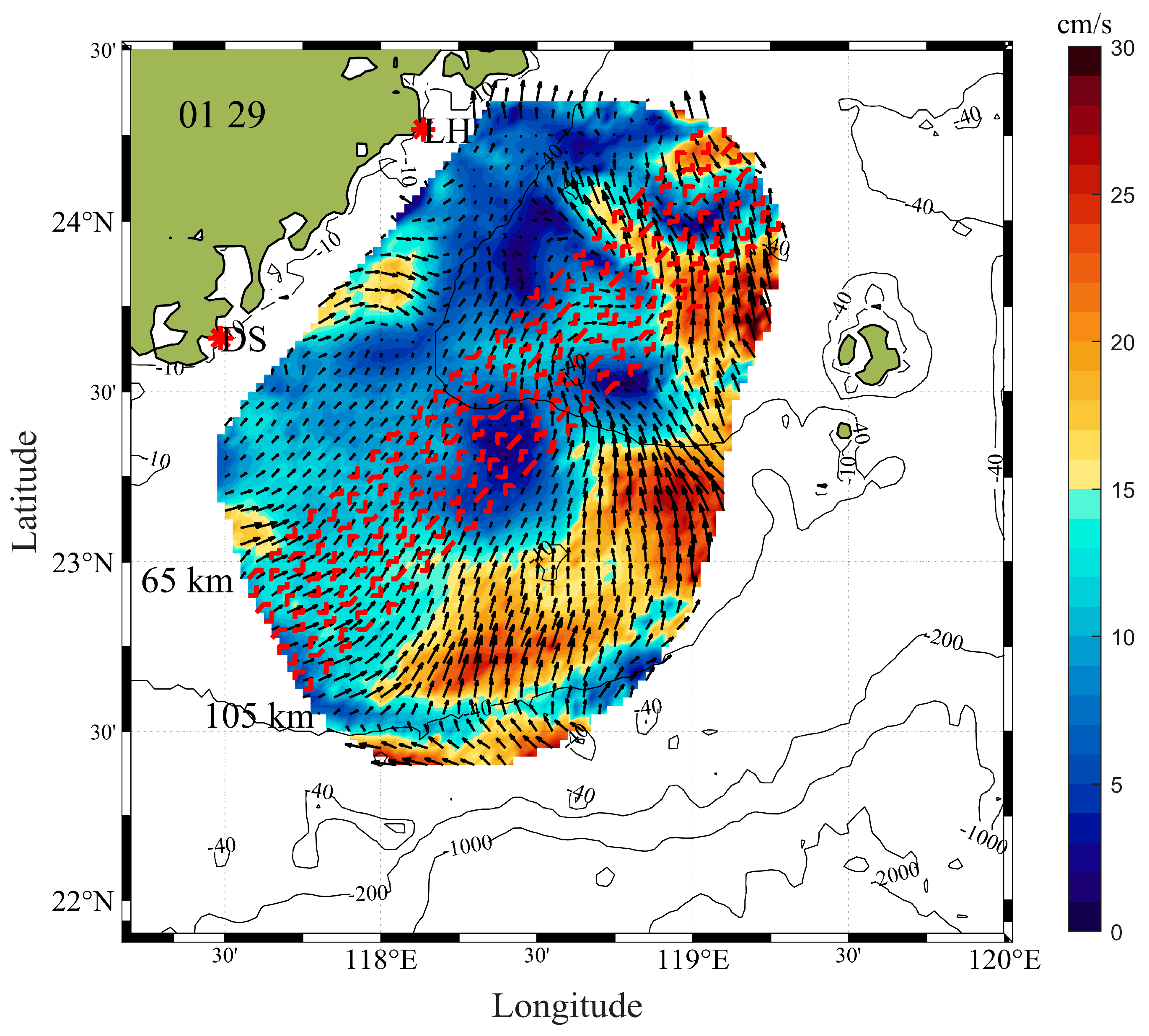
To analyze the fluctuation characteristics of the sea surface residual currents in the Taiwan Strait during the experimental period, this study selected nine adjacent transects parallel to the coastline, as indicated by the red dashed lines in Figure 7. Among these transects, the closest was located 65 km from the coast, while the farthest was 105 km, with a spacing of 5 km between each line. This configuration was chosen because a 40 km span can sufficiently cover the possible characteristic phenomena, thereby enabling the extraction of more specific and accurate features.

Figure 7. Nine equally spaced transects parallel to the coastline at 65 km–105 km offshore.

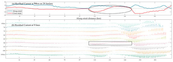
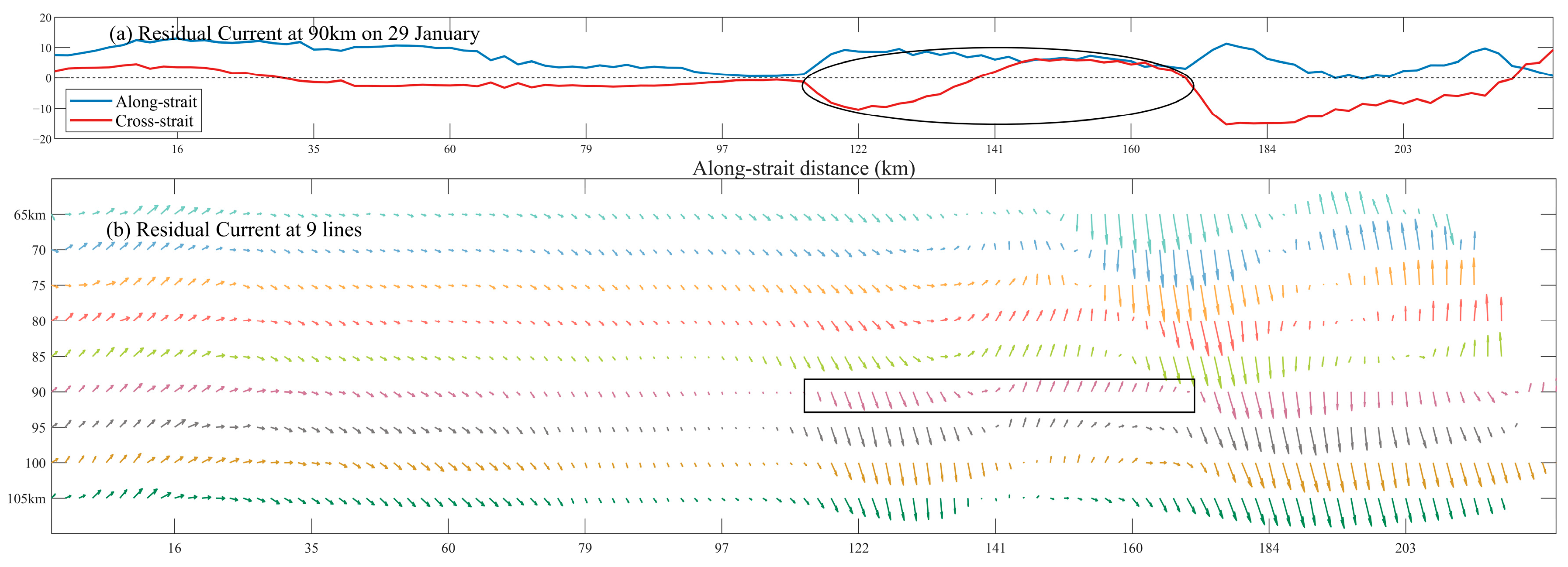
Detailed characteristics of Case 1 are presented in Figure 8, where the red dashed line spanned approximately 200 km. Figure 8a shows the residual currents at all spatial points along the 90 km offshore red dashed line at 04:00 UTC on 29 January. The blue and red curves represent the along-shore and cross-shore components of the residual currents, respectively. Along the red dashed line, from 150 km to 200 km in the southwest-to-northeast direction, the cross-shore component exhibited distinct fluctuations. These fluctuation features are more intuitively displayed within the rectangular box in Figure 8b, where the signal extends spatially over approximately one wavelength. The mean along-shore residual current velocity was 8.9 cm/s, and the actual wavelength was about 58.3 km.

Figure 8. Wave characteristics of Case 1 (29 January): (a) plots of current velocity (cm/s) against along-shore transect length, and (b) plots of cross-shore distance against along-shore transect length.

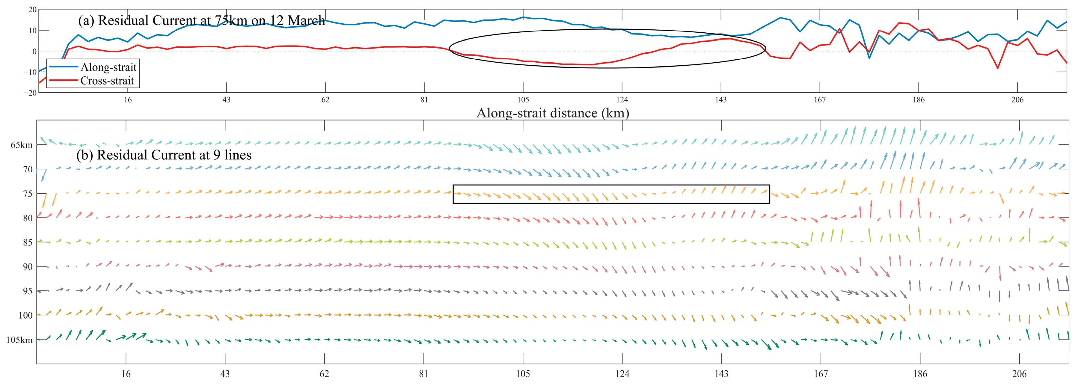
Detailed characteristics of Case 2 are presented in Figure 9. Figure 9a displays the residual currents at spatial points along the 75 km offshore red dashed line. The velocity of the cross-shore component varied significantly, but its direction changed only slightly, and the periodic directional shifts were asymmetric. Similarly, the feature marked by the rectangular box in Figure 9b was not pronounced. The mean along-shore residual current velocity was 10.9 cm/s, and the actual wavelength was approximately 65.8 km.

Figure 9. Wave characteristics of Case 2 (12 March). The meanings of the horizontal and vertical axes in (a,b) are consistent with those in Figure 8.

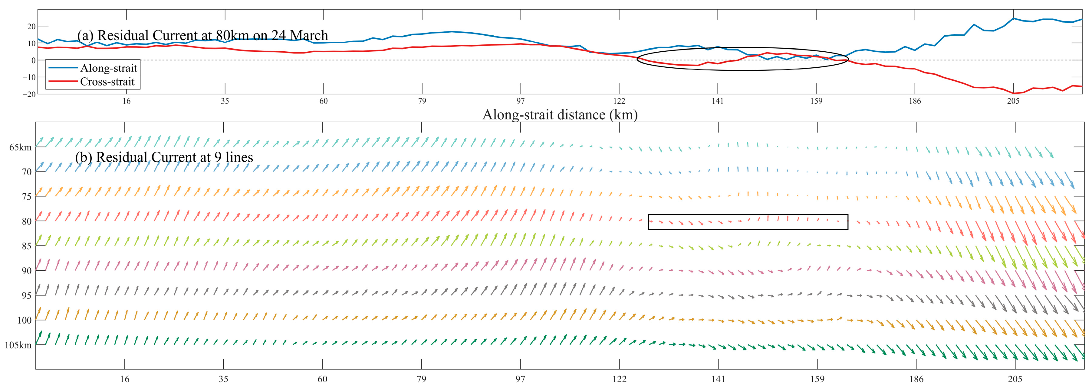
Detailed characteristics of Case 3 are presented in Figure 10. Figure 10a shows the residual currents at spatial points along the 80 km offshore red dashed line. Over the Taiwan Bank (from 60 km to 110 km in the southwest-to-northeast direction), the along-shore and cross-shore components of the residual currents exhibited a significant phase difference. Once the current surpasses beyond the Taiwan Bank, the cross-shore component begins to fluctuate and periodically reverse its direction. The current vectors within the rectangular box in Figure 10b also illustrate this feature, showing that the fluctuation extended spatially over more than one wavelength. The mean along-shore residual current velocity was 11.5 cm/s, and the actual wavelength was approximately 35.6 km.

Figure 10. Wave characteristics of Case 3 (24 March). The meanings of the horizontal and vertical axes in (a,b) are consistent with those in Figure 8.

3.2. Low-Wind Residual Current Dynamics

The results presented in Section 3.1 indicate that under low wind speed conditions, the residual current field exhibits a complex current regime shaped influenced by weak wind stress, significant inertial effects (including counter-wind currents), and seabed topography. The most prominent manifestation was the submesoscale fluctuations observed in the Xiapeng Depression area. However, the specific contributions of these factors require further clarification. To explore underlying dynamic mechanisms of the residual currents, this study analyzed the terms of the momentum equation, distinguishing the influences of different driving forces—such as wind stress, pressure gradient force, bottom friction, and the Coriolis force—on the residual current. The aim was to identify the dominant terms in the momentum balance during low wind speed periods and to elucidate the energy sources and dynamic conditions responsible for the generation of these fluctuations.

Two assumptions were considered: (1) the effect of the Earth’s curvature can be neglected in mesoscale oceanic regions; (2) seawater density is constant. Following the one-dimensional damped slab model proposed by Pollard and Millard (1970) [39], which was constructed based on observational data and numerical models, and after accounting for factors such as the Coriolis force, sea surface wind stress, and bottom friction, the momentum equations along the along-shore ($x$ axis) and cross-shore ($y$ axis) directions can be expressed as follows:

$$\begin{array}{l}\begin{array}{l}\left\{\begin{array}{l}{\displaystyle \frac{\partial u}{\partial t}}+(u{\displaystyle \frac{\partial u}{\partial x}}+v{\displaystyle \frac{\partial u}{\partial y}})-fv={\displaystyle \frac{{\tau }_{sx}}{{\rho }_{w}H}}-g{\displaystyle \frac{\partial \eta }{\partial x}}-{\displaystyle \frac{{\tau }_{bx}}{H}}\\ {\displaystyle \frac{\partial v}{\partial t}}+(u{\displaystyle \frac{\partial v}{\partial x}}+v{\displaystyle \frac{\partial v}{\partial y}})+fu={\displaystyle \frac{{\tau }_{sy}}{{\rho }_{w}H}}-g{\displaystyle \frac{\partial \eta }{\partial y}}-{\displaystyle \frac{{\tau }_{by}}{H}}\end{array}\right.\end{array}\\ \begin{array}{cccccc}\downarrow & \downarrow & \downarrow & \downarrow & \downarrow & \downarrow \\ \mathrm{Term}1& \mathrm{Term}2& \mathrm{Term}3& \mathrm{Term}4& \mathrm{Term}5& \mathrm{Term}6\end{array}\end{array}$$

(3)

The momentum equation consists of six terms on both sides of the equals sign: the current acceleration term, the local advection term, the Coriolis force term, the wind stress term, the pressure gradient force term, and the bottom friction term. Here, $u$ and $v$ are the horizontal current components in the $x$ and $y$ directions, $f$ is the Coriolis parameter, $g$ is the gravitational acceleration in m/s², $H$ is the mean ocean depth in m, and $\eta$ is the sea surface elevation in m. ${\rho }_w$ is the seawater density in kg/m³, $(u{\displaystyle \frac{\partial u}{\partial x}}+v{\displaystyle \frac{\partial u}{\partial y}})$ represents the horizontal advection of the residual current in the along-shore direction, and ${\tau }_{sx}$ denotes the wind stress on the sea surface, where the subscript $s$ indicates surface and $x$ denotes the alongshore direction. The boundary conditions:

$$\left\{\begin{array}{l}Surface(z=\eta ):{\tau }_{sx}={\rho }_{air}{C}_d{U}_{windx}^2,{\tau }_{sy}={\rho }_{air}{C}_d{U}_{windy}^2\\ Botton(z=-H):u=v=0\end{array}\right.$$

(4)

The wind stress is calculated using the formula proposed by Large and Pond (1981) [40] where ${\rho }_{air}$ is the air density (1.22 kg/m³), $C_d$ is the drag coefficient representing the transfer of wind momentum to the sea surface via wave drag, and $U_{wind}$ denotes the wind speed at 10 m above sea level. Due to the viscosity of water molecules, shear stress occurs not only at the air–sea interface but also at the ocean bottom. Here, ${\tau }_{bx}$ represents the bottom stress vector. In analyzing the sea surface circulation of the Taiwan Strait using the Princeton Ocean Model (POM), Oey (2014) [13] treated the strait as a channel with a fixed bottom depth $H$ and parameterized the bottom stress vector as follows:

$${\tau }_b=RH{U}_{cur}$$

(5)

Here, $R$ is set as a fixed drag coefficient (also referred to as an empirical damping coefficient, with units of s⁻¹) in this study, with a value of $R=1.43\times {10}^{-5}$ s⁻¹ [38,41].

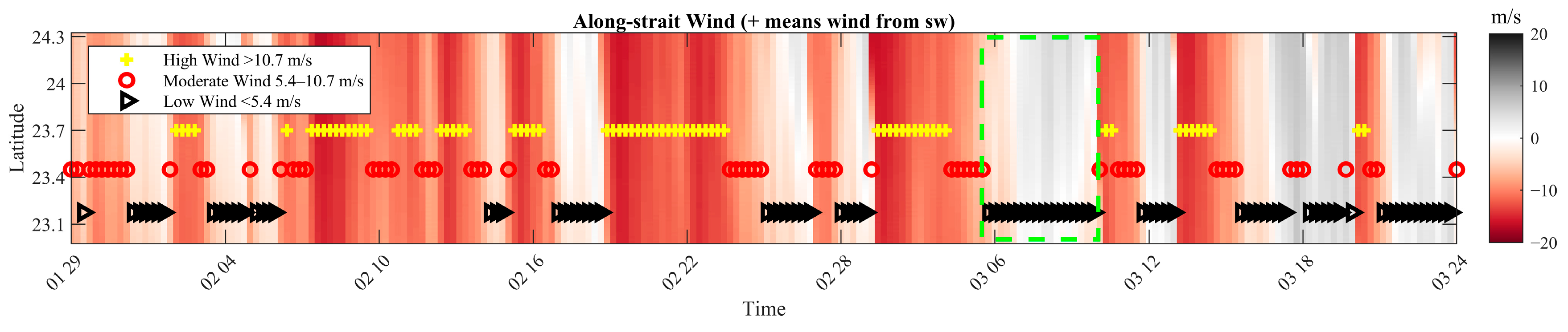
The along-shore wind speed distribution was plotted using all spatial points along the 75 km offshore red dashed line in Figure 7, as shown in Figure 11. The latitudinal range extended from 22.5° N to 24.3° N. The along-shore component of the wind vectors was approximately uniform across the entire latitude range at any given time. The green dashed box marks the longest continuous low wind speed period, spanning from 06:00 on 6 March to 11:00 on 10 March.

Figure 11. Along-shore wind speeds at 75 km offshore, the x-axis represents the period from 29 January 2013 to 24 March 2013. Reproduced from [38].

We calculated the variance of each term in the momentum equations at every spatial point within the computational grid and mapped their spatial distribution. Variance describes the amplitude of temporal fluctuations in a random variable, allowing for an assessment of whether each momentum term remains stable during the low wind speed period indicated by the green dashed box.

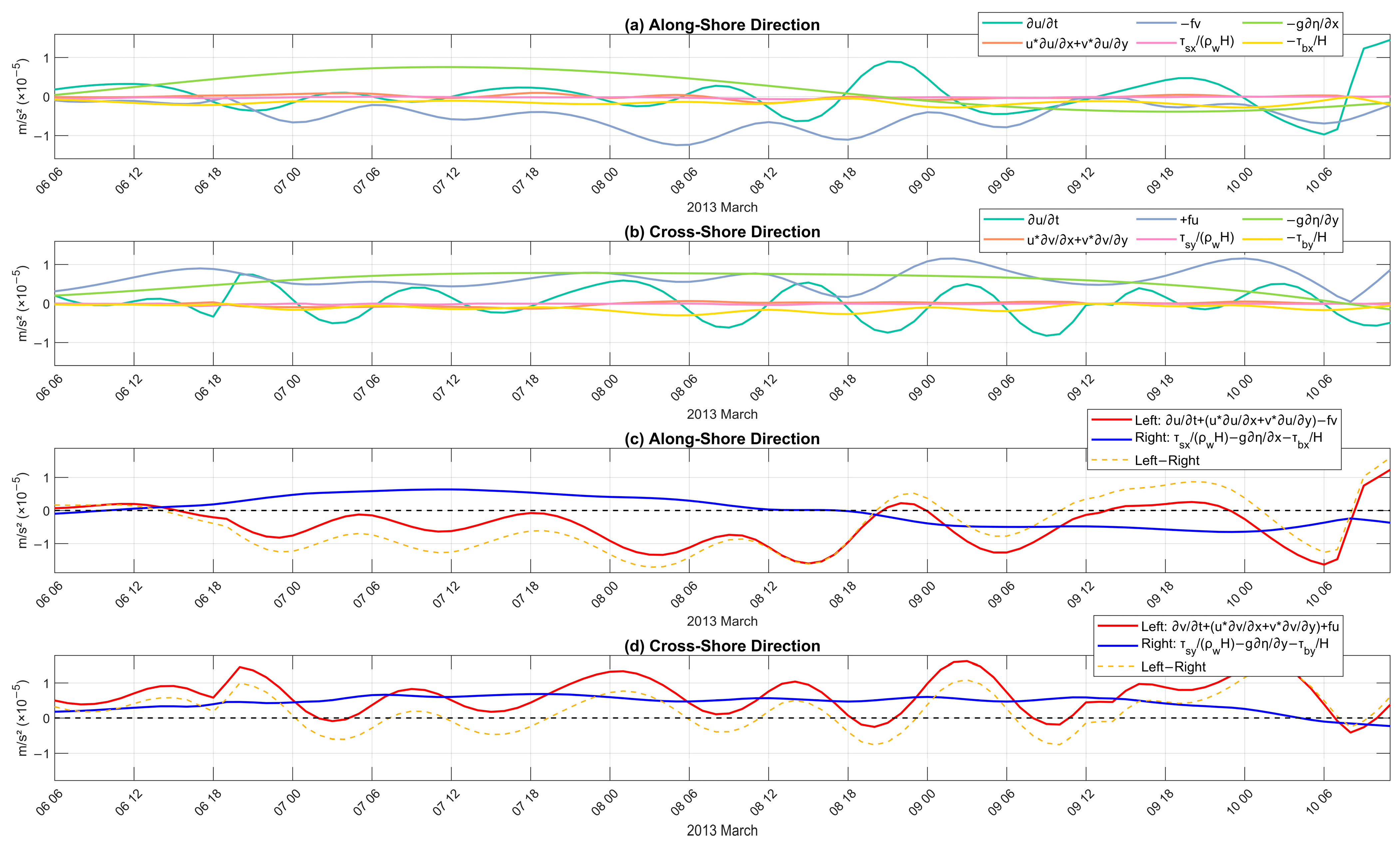
Figure 12 presents the temporal evolution of each term in the momentum equation, as well as the left side, right side, and their difference at Point A (see Figure 1, located in the Xiapeng Depression north of the Taiwan Bank) during the low-wind period. From Figure 12a,b, it can be discerned that the acceleration term, the Coriolis term, and the pressure gradient term exhibited substantially larger fluctuations in both the along-shore and cross-shore directions compared to the advection term, wind stress term, and bottom friction term. The latter three terms remained near zero with only minor perturbations, indicating that the acceleration, Coriolis, and pressure-gradient terms dominate the momentum balance. To further assess the budget of the momentum equation, the residuals between the left side and right side were calculated to evaluate the closure of the balance. For both the alongshore and cross-shore directions of Equation (3), the left side, right side, and their differences are shown in Figure 12c,d. The temporal variation of the difference closely followed, or even coincided with that of the left side, confirming that the acceleration and Coriolis terms exert a dominant influence on the momentum balance across the study area throughout the low-wind period. The time-mean absolute values of the alongshore and cross-shore residuals were $0.775\times {10}^{-5}$ m/s² and $0.467\times {10}^{-5}$ m/s², respectively, indicating that the momentum balance is satisfied.

Figure 12. Time series of each momentum term in (a) along-shore and (b) cross-shore directions at A (units: m/s²). Time series of the sum on the left and right sides of Equation (3) and their difference in (c) along-shore and (d) cross-shore directions, the x-axis represents the period from 6:00 6 March 2013 to 10:00 10 March 2013.

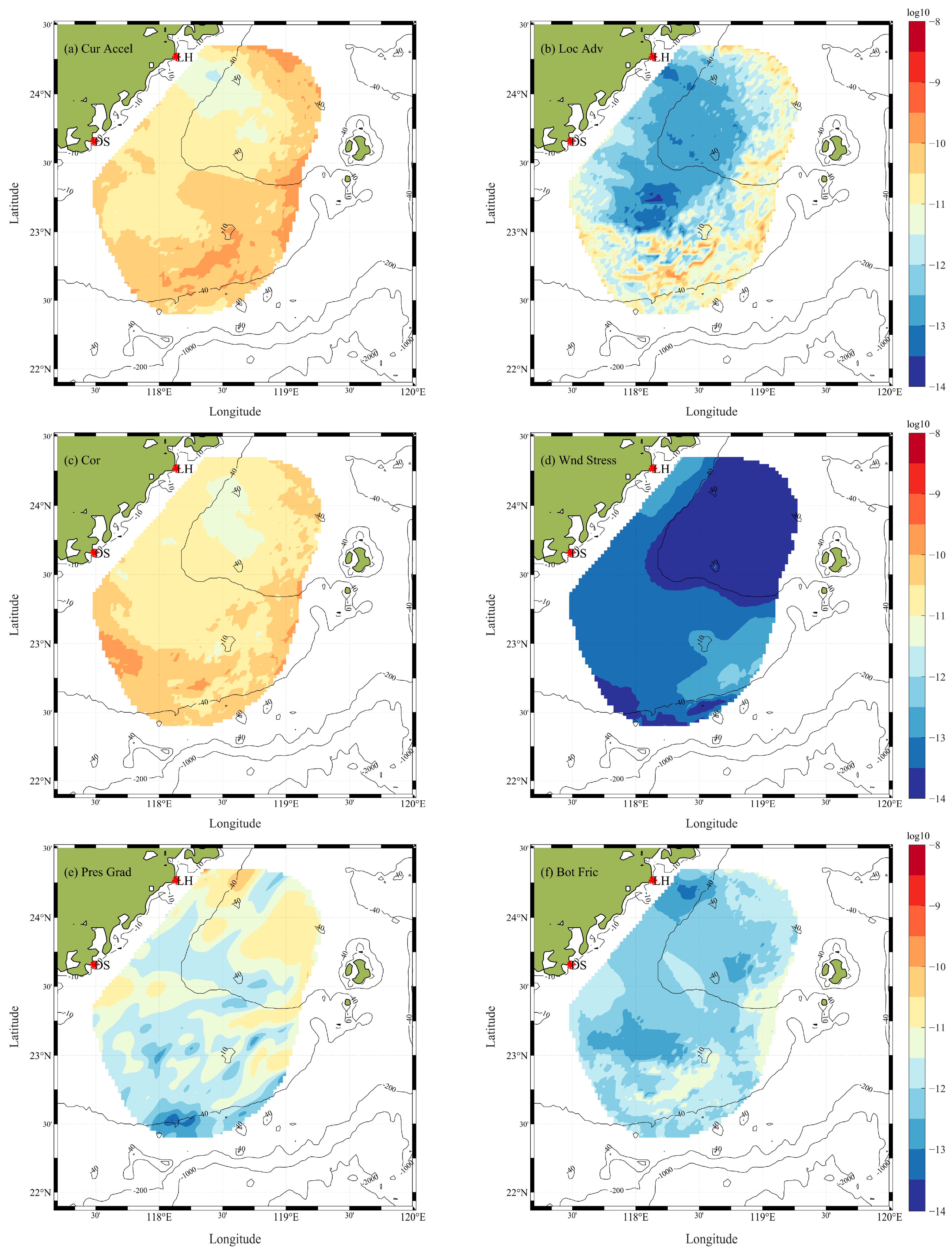
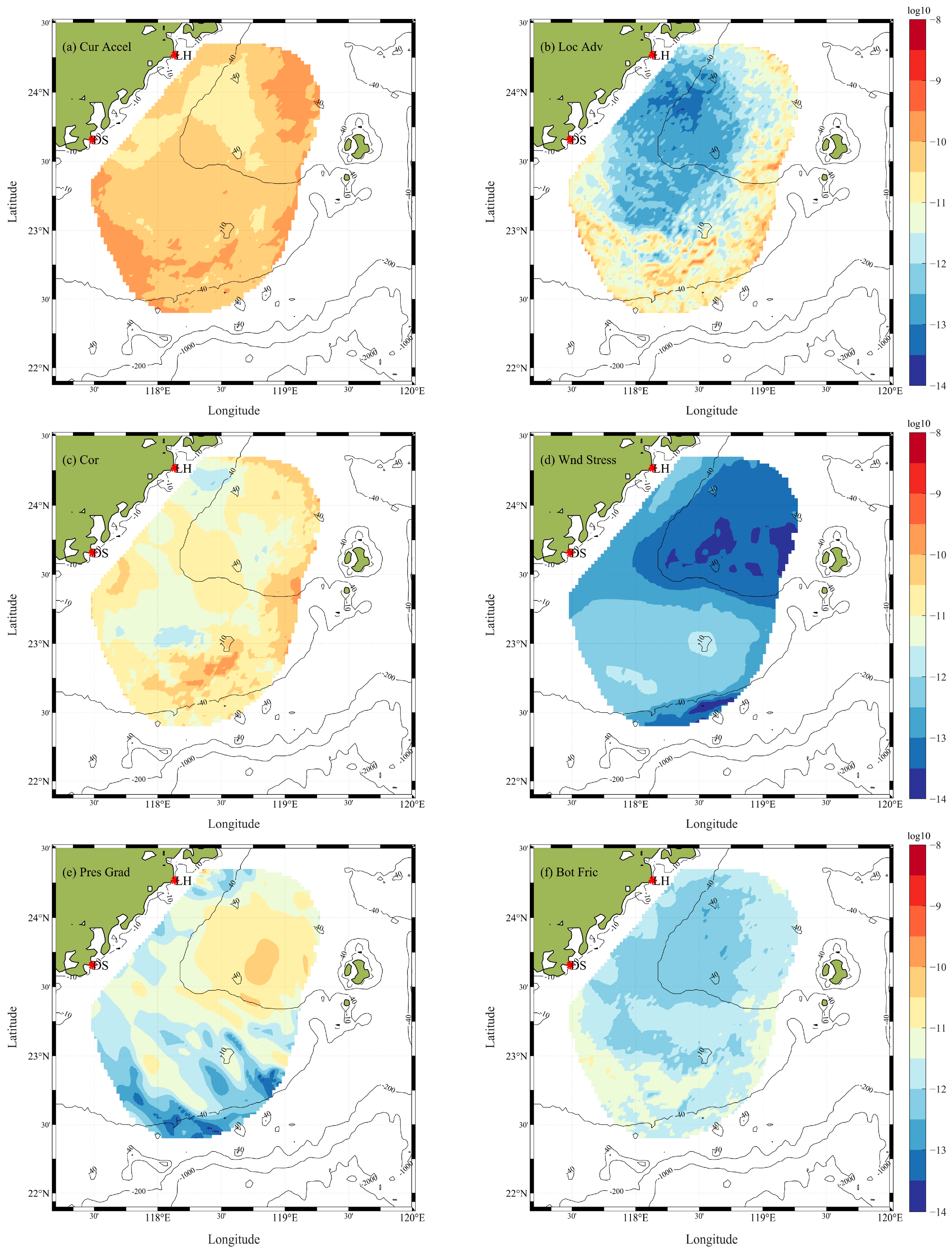
In the cross-shore direction (Figure 13), the variance of the Coriolis force term was the largest, followed by that of the acceleration term. This indicates that the current velocity across the entire region is temporally unsteady, which in turn leads to substantial temporal variation in the acceleration term (the first-order time derivative of velocity). These two terms are the primary factors influencing the momentum balance during low wind periods. In contrast, the variances of the nonlinear advection term and the pressure gradient force term were at least two orders of magnitude smaller. This is because, under low wind conditions, the residual current is no longer in a wind-dominated quasi-steady equilibrium state but is transitioning from a broad inertial adjustment phase toward a locally time-averaged quasi-steady current regime. During this transition, the contribution of wind-driven current is low, and the small wind waves result in minimal sea surface height variability. In the Taiwan Bank and Xiapeng Depression areas, the variance of the bottom friction term was second only to that of the pressure gradient force term, indicating that bottom friction exerts a modest, though not dominant, influence on the regulation of residual currents in these shallow waters under low winds. The wind stress term exhibited the smallest variance, indicating that its contribution to and influence on the momentum balance is negligible.

Figure 13. Spatial distribution of momentum equation term variances in the cross-shore direction: (a) acceleration term, (b) local advection term, (c) Coriolis force term, (d) wind stress term, (e) pressure gradient force term, and (f) bottom friction term.

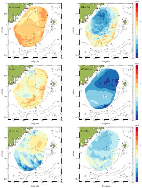
In the along-shore direction (Figure 14), the variance distribution characteristics of the nonlinear advection term and the bottom friction term were similar to those in the cross-shore direction, with the wind stress term being negligible. The Coriolis force term and the acceleration term exhibited the largest variances, continuing to play a dominant role in the momentum balance. The variance of the pressure gradient force showed a region of relatively high values north of the Taiwan Bank, indicating that during the low wind speed period, the along-shore component of the sea surface wind field was significant. This corresponded to an increase in the variance of the wind stress term by approximately one order of magnitude. The prevailing southwesterly winds caused some accumulation of water along the Taiwan Bank in this direction, leading to a discernible sea surface height gradient.

Figure 14. Spatial distribution of momentum equation term variances in the along-shore direction: (a–f) denote the same terms as in Figure 13.

4. Discussion

During low-wind-speed periods, the spatiotemporal characteristics of sea surface residual currents in the Taiwan Strait primarily manifest as submesoscale fluctuations occurring in the Xiapeng Depression area. We attempt to explain the underlying dynamic mechanism of these fluctuations.

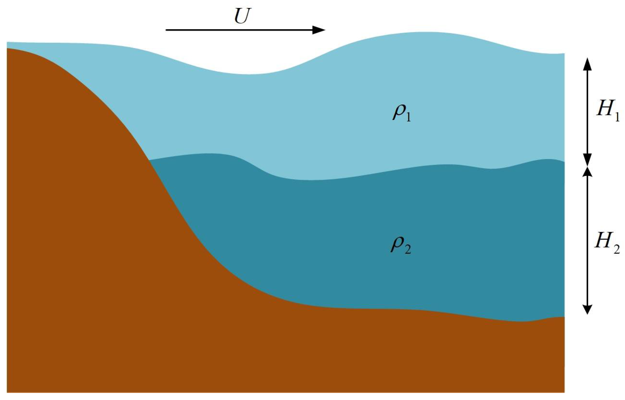
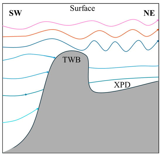
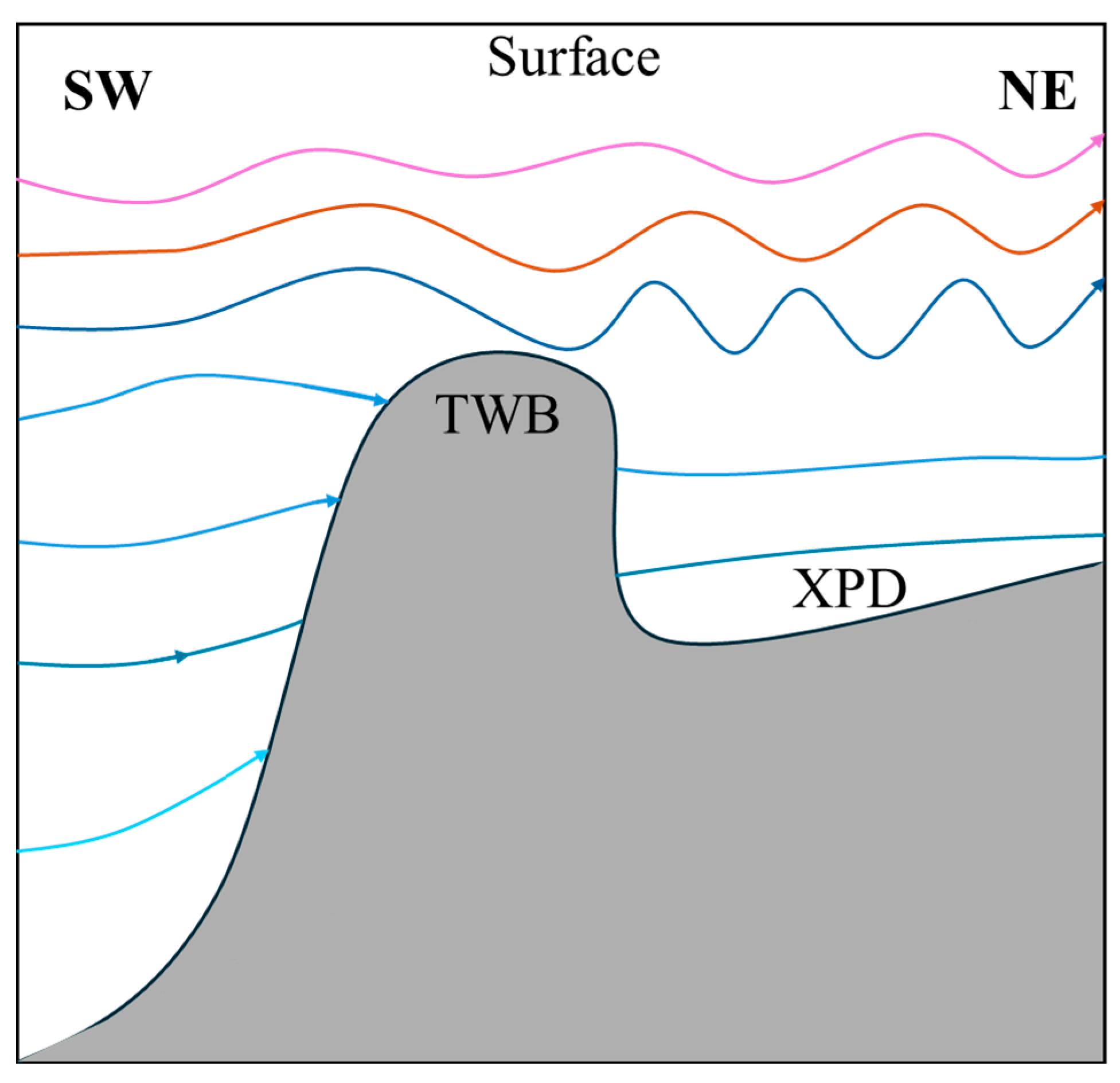
Previous studies have provided experimental evidence for the influence of internal waves on surface currents. Luo et al. (2021) [42] employed particle methods in their experiment, simulating the flow field by tracking the motion of discrete fluid particles. This approach is well-suited for directly outputting and visualizing the trajectories of individual fluid particles beneath the wave field, as well as the three-dimensional velocity field within the fluid. Meng et al. (2017) [43] constructed a two-layer stratified fluid in a three-dimensional wave tank and used particle image velocimetry (PIV) to perform direct, quantitative experimental observations of the surface flow field (velocity, divergence, vorticity) induced by internal waves generated by a horizontally moving sphere. Their work revealed that the surface flow field driven by internal waves exhibited a V-shaped convergent-divergent structure resembling the crest line of a Kelvin wave. Building on these advances, considering the geographical location where these sea surface residual current fluctuations appeared, the topography of the Taiwan Bank, and factors such as the counter wind current, it is hypothesized that these submesoscale fluctuation features result from internal lee waves propagating to the surface through nonlinear interactions. Internal lee waves are quasi-steady internal gravity waves generated by the interaction between ocean currents and steep seabed topography, which enhance turbulence and mixing in the ocean when they break [44]. Internal lee waves can also generate near-surface currents capable of significantly modulating the surface wave field within a two-layer oceanic stratification [45]. The energy of lee waves originates from quasi-steady currents, and their triggering condition is the current passing over significantly undulating seabed terrain [46]. The waters surrounding the Taiwan Bank satisfy these conditions: the Taiwan Bank has an average water depth of about 20 m, and its southern flank is an exceptionally steep continental slope where the ocean depth drops rapidly by over 2500 m. Given this specific topographic configuration, if a barotropic current flows from south to north (or northeast) across the Taiwan Bank, its interaction with the steep seabed topography is likely to generate lee waves in the area north (or northeast) of the Taiwan Bank (as illustrated in Figure 15).

Figure 15. Schematic diagram of Lee waves generated by current–topography interaction, the arrow indicates the direction of current.

To quantitatively investigate the influence of topography on residual currents, a theoretical analysis of the submesoscale fluctuations affecting the sea surface current was conducted. A two-layer stratified ocean model was constructed for simulation. Meanwhile, HFSWR observations of the residual currents and the winter stratification conditions in the southwestern Taiwan Strait were incorporated as reference. Relevant wave parameters were computed and subsequently compared with observational data for validation.

Based on linear wave theory and assuming the seawater is homogeneous and inviscid, and considering that the Rossby number for large-scale motions is much less than 1, the nonlinear terms can be neglected [47]. This leads to the following shallow water equations:

$$\left\{\begin{array}{l}{\displaystyle \frac{\partial u}{\partial t}}-fv=-g{\displaystyle \frac{\partial \eta }{\partial x}}\\ {\displaystyle \frac{\partial v}{\partial t}}+fv=-g{\displaystyle \frac{\partial \eta }{\partial y}}\\ {\displaystyle \frac{\partial \eta }{\partial t}}+H({\displaystyle \frac{\partial u}{\partial x}}+{\displaystyle \frac{\partial v}{\partial y}})=0\end{array}\right.$$

(6)

For further simplification, considering variations only in the $x$ direction, the wave solution for this homogeneous problem is obtained as follows:

$$\left\{\begin{array}{l}u=U{e}^{i(kx-\omega t)}\\ v=V{e}^{i(kx-\omega t)}\\ \eta =N{e}^{i(kx-\omega t)}\end{array}\right.$$

(7)

where $\omega$ is the angular frequency of ocean waves. Substituting into the linear shallow water equations yields:

$$\left\{\begin{array}{l}-i\omega U-fV=-igkN\\ -i\omega V+fU=0\\ -i\omega N+ikHU=0\end{array}\right.$$

(8)

Other than $\omega =0$, the solution is expressed in terms of the wavenumber $k$ as:

$${\omega }^2=f^2+gH{k}^2$$

(9)

This is the dispersion relation of the wave, which can be alternatively expressed as:

$$\left\{\begin{array}{l}{k}^2={\displaystyle \frac{{\omega }^2-f^2}{gH}}\\ V={\displaystyle \frac{fU}{i\omega }}\\ N={\displaystyle \frac{kHU}{\omega }}\end{array}\right.$$

(10)

Assume that the $x$ axis is aligned with the along-shore direction pointing northeast. The velocity components $u$ and $v$ can thus be expressed as the sum of a steady component ($\overline{u}$) and a perturbation component ($\overline{v}$):

$$\left\{\begin{array}{l}u=\overline{u}+u^{\prime }\\ v=\overline{v}+v^{\prime }\end{array}\right.$$

(11)

Here, the phase speed of surface inertial gravity waves in the rotating shallow water equations is:

$$c_p={\displaystyle \frac{\omega }{k}}=\sqrt{gH+{\displaystyle \frac{f^2}{k^2}}}$$

(12)

This yields:

$$k^2={\displaystyle \frac{f^2}{{c_p}^2-gH}}$$

(13)

When a steady current exists in the surface layer, the phase speed of the wave will be affected by the current velocity [48]. Assuming the wave propagates in the same direction as the mean current (both along the $x$ direction), the actual phase speed of the wave increases. Based on the Benjamin–Ono (BO) equation, a classical integrable model describing interfacial waves in a two-layer fluid of infinite depth, the study by Flamarion and Pelinovsky highlights that the Ursell parameter $U_r$ is a key dimensionless number governing the relative strength of nonlinearity and dispersion. In real oceanic environments, variations in critical factors such as background current intensity, stratification strength, or topographic slope can influence the spatiotemporal distribution of surface residual currents and the generation of submesoscale fluctuations [49]. Specifically, the actual phase speed $U_r$ can be expressed as the vector sum of the free wave phase speed under shallow water conditions $c_0=\sqrt{gH}$ and the component of the current velocity $u$ in the direction of wave propagation, i.e., $U_r=c_0+u$ [50].

Equation (13) can be revised as:

$$k^2={\displaystyle \frac{f^2}{{U_r}^2-gH}}$$

(14)

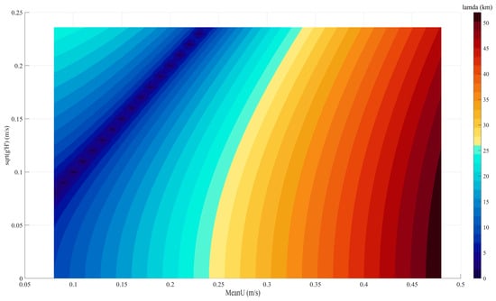
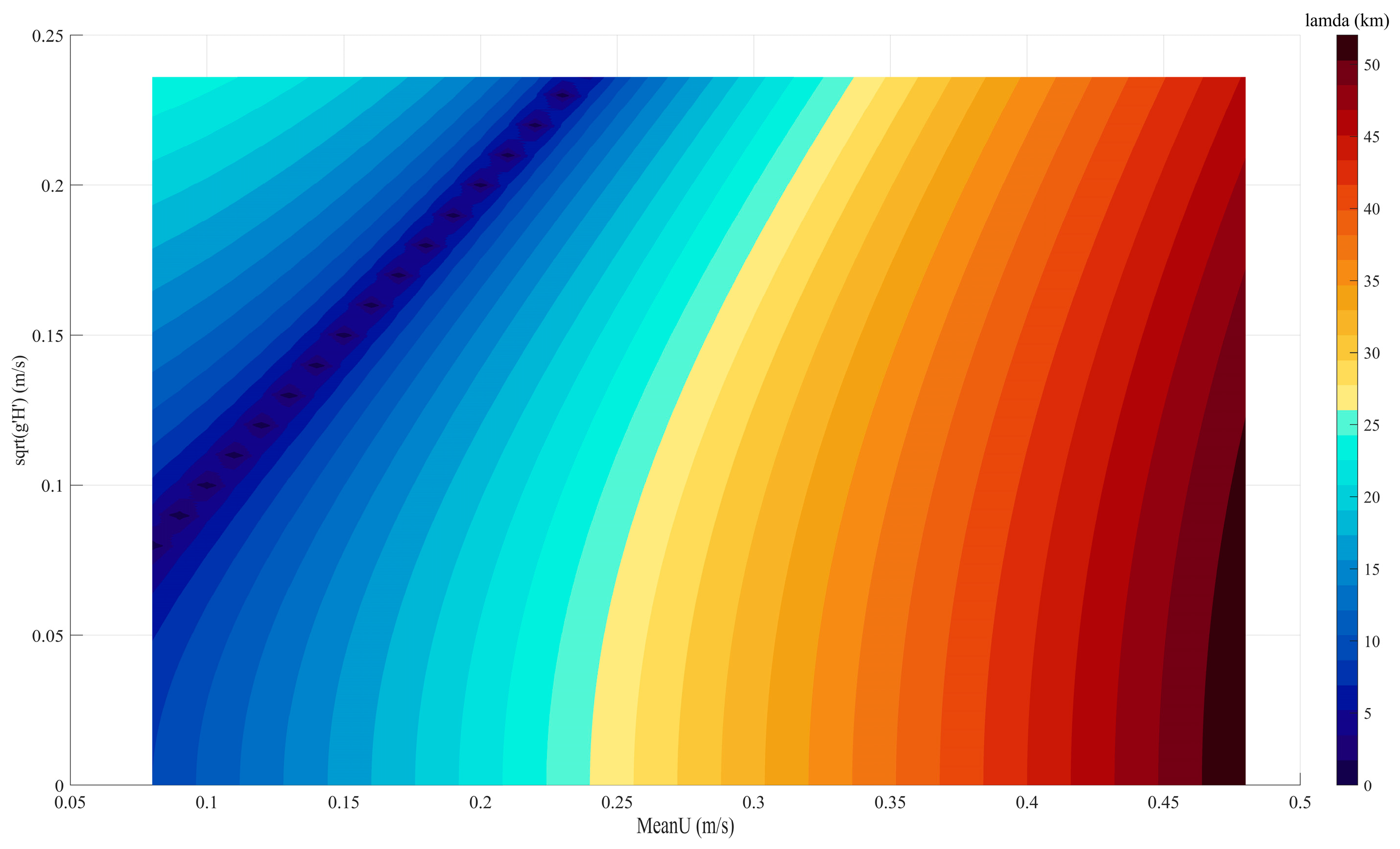
The relationship between the wavelength $\lambda =2\pi /k$ of these rotationally-modified gravity waves, the phase speed of the rotationally modified surface gravity waves, and the intensity of the quasi-steady current is illustrated in Figure 16. The wavelength reaches a minimum when the reduced phase speed approaches the steady current velocity. For a fixed modified phase speed, the wavelength exhibits a non-monotonic trend with increasing steady current, decreasing first and then increasing.

Figure 16. Relationship between steady current, wavelength, and phase speed of rotationally modified gravity waves.

Typically, seawater density increases non-uniformly with depth, and most ocean interiors exhibit a vertically stratified structure with density variations [51]. Considering the weak stratification present in the southwestern Taiwan Strait during winter [11], it was assumed that seawater density remains uniform at all depths except at the fluid interface where stratification occurs (as shown in Figure 17). The densities of the upper and lower layers are ${\rho }_1$ and ${\rho }_2$, and their depths are $H_1$ and $H_2$, respectively [52]. In this case, the reduced gravity can be calculated as follows:

$$g^{\prime }=g{\displaystyle \frac{\Delta \rho }{\rho }}\approx g{\displaystyle \frac{{\rho }_2-{\rho }_1}{{\rho }_1}}$$

(15)

Effective ocean depth:

$$H^{\prime }={\displaystyle \frac{H_1{H}_2}{H_1+H_2}}=1/({\displaystyle \frac{1}{H_1}}+{\displaystyle \frac{1}{H_2}})$$

(16)

Based on observational data from References [11,53,54], the following values were adopted for the Xiapeng Depression area: $H^{\prime }\approx$ 14.58 m, $\Delta \rho \approx$ 0.1 kg/m³, and $\rho \approx$ 1024.5 kg/m³.

Equation (14) can be revised as:

$$k^2={\displaystyle \frac{f^2}{{U_r}^2-g^{\prime }{H}^{\prime }}}$$

(17)

Figure 17. Two-layer stratified ocean model (denotes the steady current velocity).

Figure 17. Two-layer stratified ocean model (denotes the steady current velocity).

When only the quasi-steady current in the $x$ direction is considered, it is assumed that there exists a combined solution consisting of a real part and an imaginary part related to the governing equation for the steady current induced wave. The corresponding complex solution is then obtained by taking either the real or the imaginary part. The complete solution is composed of a particular solution and a homogeneous solution, which are summed to satisfy the boundary conditions. If a spatial solution for $u$ and $v$ exists, it can be expressed as:

$$\left\{\begin{array}{l}u=\mathrm{Re}\left\{\overline{u}+A{e}^{i(kx-\omega t)}\right\}\\ v=\mathrm{Re}\left\{-{\displaystyle \frac{ifA}{k\overline{u}}}{e}^{i(kx-\omega t)}\right\}\end{array}\right.$$

(18)

Here, $A$ is the amplitude of the perturbation. The ratio of the amplitude of $u$ to that of $v$ is then:

$${\displaystyle \frac{amplitude(u^{\prime })}{amplitude(v^{\prime })}}={\displaystyle \frac{k\overline{u}}{f}}={\displaystyle \frac{\omega }{f}}$$

(19)

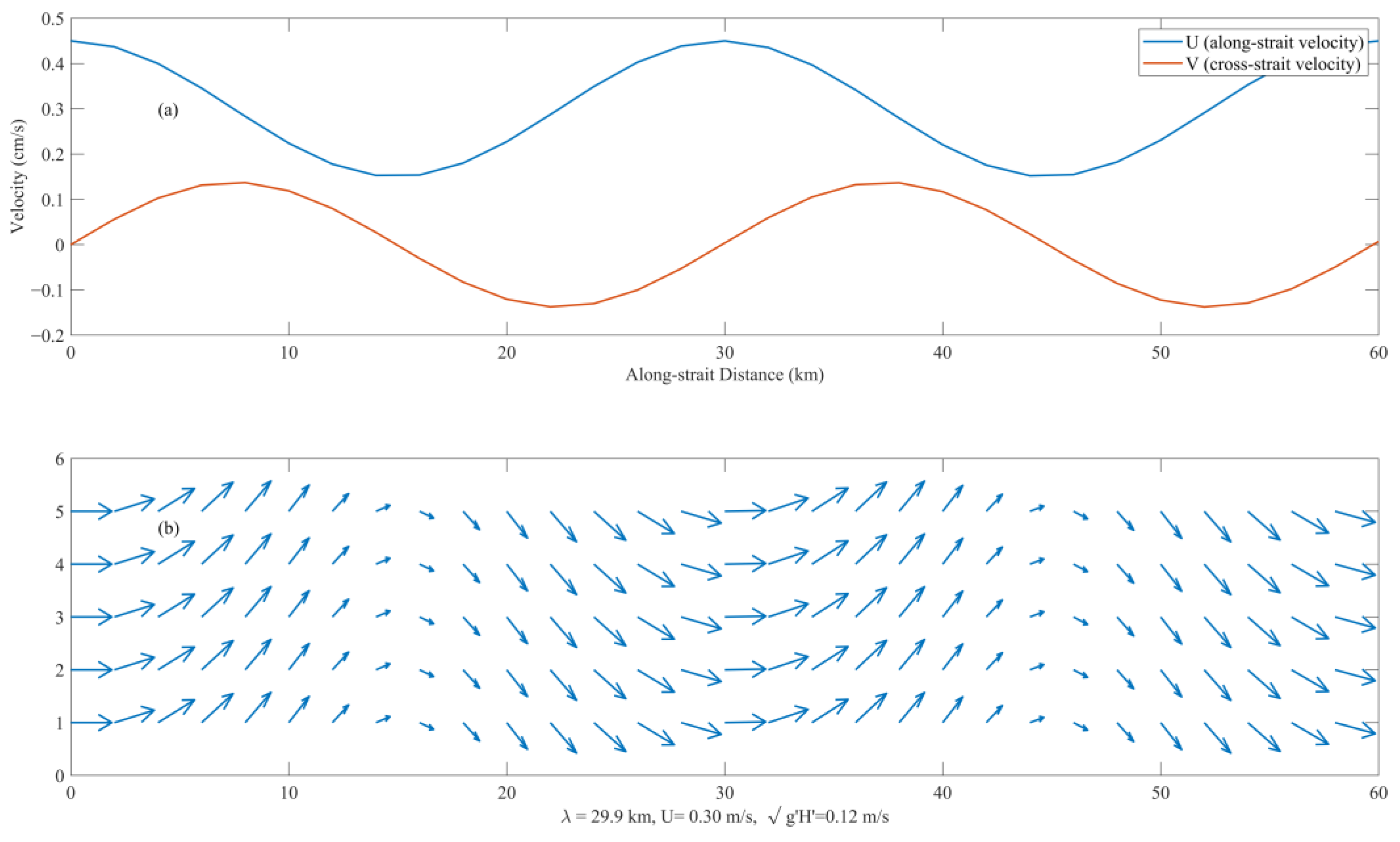
When the along-shore quasi-steady current $\overline{u}$ = 0.3 m/s, the variations of the current in the along-shore and cross-shore directions are shown in Figure 18. In Figure 18a, the blue and orange curves represent the along-shore and cross shore components of the residual current, respectively. The along-shore component remained consistently positive, indicating a persistent northeastward current; in contrast, the cross-shore component exhibited continuous directional reversals. Figure 18b displays the residual current fluctuations across consecutive spatial points, with a wavelength of approximately 30 km, which fell within the submesoscale range.

Figure 18. Schematic diagram of residual current fluctuations ($\overline{u}$ = 0.3 m/s). Model and simulate the cases from Figure 8, Figure 9 and Figure 10, (a) plots of current velocity against along-strait direction, and (b) plots of cross-shore distance against along-shore transect length.

By assuming a two-layer stratified ocean model based on the characteristics of residual current fluctuations (rotationally-modified gravity waves) and combining observations of counter-wind current from HFSWR with the unique topography of the Taiwan Bank, this study sought to elucidate the physical significance of the counter-wind current fluctuation features. Based on theoretical analysis and model simulations, the surface residual current fluctuations are jointly influenced by the Coriolis force and modified gravity. They remain constant in the direction of the steady current (along-shore direction) while periodically reversing in the cross-shore direction.

In Case 1, the steady current velocity was 20.7 cm/s. According to the two-layer stratified ocean model, the corresponding maximum wavelength was 18.4 km, while the observed wavelength was about 58.3 km. In Case 2, with a steady current velocity of 22.7 cm/s, the model yielded a maximum wavelength of 21.1 km, whereas the observed wavelength was approximately 65.8 km. For Case 3, the steady current velocity was 23.3 cm/s, and the model gave a maximum wavelength of 21.3 km, but the observed wavelength was around 35.6 km. In all three cases, the observed wavelengths exceeded the simulated wavelengths from the model. To further evaluate the robustness of the proposed model given the results obtained above, a sensitivity analysis was conducted focusing on two key parameters closely related to oceanic stratification in the wavelength calculation: the reduced gravity $g^{\prime }$ and the effective depth $H^{\prime }$. These two quantities reflect, respectively, the density contrast between the two layers and the layer thicknesses in the two-layer ocean model, where $g^{\prime }\propto \Delta \rho$ (with $a=g/{\rho }_0$ being constant). The density difference $\Delta \rho$ was varied from 0.05 kg/m³ to 0.15 kg/m³ at intervals of 0.05 kg/m³, and $H^{\prime }$ was varied from 5 m to 30 m at intervals of 5 m. For each of the three cases, the corresponding wavelength was calculated for every combination of $\Delta \rho$ and $H^{\prime }$, yielding a sensitivity analysis table for the wavelength variations (Table 1).

Table 1. Sensitivity analysis of wavelength ($\lambda$) from Case 1 to Case 3.

${\mathit{g}}^{\prime }{\mathit{H}}^{\prime }\propto \Delta \mathit{\rho }{\mathit{H}}^{\prime }$ (m2/s2)	Case 1: $\mathit{\lambda }$ (km)	Case 2: $\mathit{\lambda }$ (km)	Case 3: $\mathit{\lambda }$ (km)
0.05 × 5	14.0	15.7	14.4
0.10 × 5	15.4	17.2	15.8
0.15 × 5	16.4	18.3	16.7
0.05 × 10	15.4	17.2	15.8
0.10 × 10	17.2	19.2	17.7
0.15 × 10	18.5	20.5	19.0
0.05 × 15	16.4	18.3	16.9
0.10 × 15	18.5	20.5	19.0
0.15 × 15	20.0	22.1	20.5
0.05 × 20	17.2	19.2	17.7
0.10 × 20	19.5	21.6	20.0
0.15 × 20	21.1	23.3	21.7
0.05 × 25	18.0	19.9	18.4
0.10 × 25	20.4	22.5	20.9
0.15 × 25	22.1	24.3	22.6
0.05 × 30	18.5	20.5	19.0
0.10 × 30	21.1	23.3	21.7
0.15 × 30	22.9	25.2	23.5

As shown in Table 1, 18 sets of analytical values were obtained for each case. For Case 1, the maximum wavelength reached 22.9 km, occurring when both $\Delta \rho$ and $H^{\prime }$ attained relatively large values—a scenario corresponding to strong oceanic stratification. However, this does not align with the weak stratification conditions typical of the study area in winter [11]. The minimum wavelength for Case 1 was 14.0 km, corresponding to a density difference of 0.05 kg/m³ but an effective depth of only 5 m. This value deviates considerably from both the actual water depth in the region and the effective depth derived from layer thicknesses in the stratified water column. Among the remaining 16 combinations, the wavelength fluctuated within ±3 km relative to the reference value of 18.4 km, which was a relatively minor variation given the characteristic scales of submesoscale fluctuations. For Cases 2 and 3, the wavelength variations also remained within ±5 km of the original predicted values, indicating no substantial deviation. These results further demonstrate the robustness of the model.

All of the above analysis constitutes a preliminary discussion of the model. Potential reasons for these discrepancies were analyzed as follows. First, the assumed model contains certain limitations. The free waves radiating from the interfacial waves within the stratified layer to the sea surface, thereby inducing submesoscale perturbations in the surface currents, involve nonlinear physical oceanographic processes and wave-current interactions that require more in-depth experimental investigation or additional observational data for robust support. Simply assuming a barotropic two-layer stratified ocean model compresses and simplifies this process, neglecting the “stretching” of waveforms due to long-wave propagation in baroclinic modes and the energy dissipation of short waves caused by turbulent friction. These omissions contribute to the discrepancies observed between the model predictions and actual measurements. Nevertheless, sensitivity analysis indicates that the model remains relatively robust. Second, the Taiwan Bank has a broad and complex topography that is difficult to fully simplify as a single submarine ridge structure. Discrepancies exist between the model assumptions and the real marine environment, where the intensity of ocean stratification is not spatially uniform. Third, strong offshore currents are present east of the Taiwan Bank, and eddy structures have been observed near the western coast, indicating that the surface current field can be readily influenced by surrounding currents. Additionally, under low wind speed conditions (≤5 m/s), the direct forcing from local wind stress is substantially reduced. In such scenarios, ocean surface currents can be significantly modulated by non-local forcings, among which swell (long-period waves generated by distant storms) plays a prominent role [55]. Swell contributes to the surface momentum balance through radiation stress gradients, driving Stokes drift and modifying the effective wind stress acting on the ocean surface layer [56]. The observed counter-wind current and the associated submesoscale fluctuations during monsoon relaxation periods may partly derive energy from this swell-related momentum flux, particularly given that the Taiwan Strait is open to swell propagation from both the Pacific Ocean and the South China Sea. While the present study focused on the wind–current and current–topography interactions mechanism, the potential contribution of swell to the residual current field, especially in the absence of strong local winds, warrants consideration. Future studies incorporating directional wave spectrum data would be valuable for disentangling the relative contributions of local wind stress and swell radiation stress to the momentum budget described in Section 3.2.

5. Conclusions

Based on high spatiotemporal resolution ocean current data observed by High-Frequency Surface Wave Radar and combined with ERA5 reanalysis wind fields and the OTIS tidal model, this study revealed the spatiotemporal characteristics of surface residual currents in the southwestern Taiwan Strait under low wind speed conditions (≤5 m/s) and analyzed their underlying dynamic mechanisms.

During the winter monsoon relaxation period, under low wind speeds, the surface residual current manifests as a counter-wind current (direction opposite to the wind). This current, upon crossing the Taiwan Bank, excites submesoscale fluctuations with periodic oscillations in the Xiapeng Depression area. Three representative cases were selected: at 04:00 UTC on 29 January, 18:00 UTC on 12 March, and 06:00 UTC on 24 March, with along-shore residual current velocities of 8.9 cm/s, 10.9 cm/s, and 11.5 cm/s, respectively. These fluctuations propagated in the along-shore direction, with wavelengths ranging from 35.6 km to 65.8 km, spanning spatially over about one to two wavelengths, and lasting approximately 6 to 12 h.

Through the analysis of the temporal variance of each term in the momentum equation for both the along-shore and cross-shore directions, it was found that during low wind speed periods, the Coriolis force term and the acceleration term dominated in both orthogonal directions, with their dominance being most pronounced in the cross-shore direction. The bottom friction and nonlinear advection terms play secondary roles, while the contribution of the wind stress term is minimal. This indicates that the current field has not yet reached a state of geostrophic balance and is in a critical transitional phase from inertial adjustment toward quasi geostrophy. Such non steady characteristics provide the necessary energy source and dynamic conditions for the subsequent generation of fluctuations.

In Section 4, by integrating geographical location, topographic gradient, and current direction, it is hypothesized that the submesoscale fluctuations described above are internal Lee waves excited by the nonlinear interaction of the residual current crossing the Taiwan Bank with the seabed topography. Their energy radiates upward from deeper layers and manifests as observable periodic perturbations in the surface current field through vertical momentum transfer. A two-layer stratified rotationally-modified gravity wave model was constructed to simulate an approximate structure of the observed fluctuations. However, a discrepancy of 1.5 to 3 times existed between the simulated and observed wavelengths on the spatial scale. This suggests that the Taiwan Bank topography is broad and complex, and the intensity of ocean stratification is not spatially uniform. The assumption of homogeneous stratification introduces a certain degree of deviation, indicating the need to develop a stratification model that more closely approximates the real marine environment. Furthermore, the current analysis relies primarily on HFSWR surface current data and ERA5 reanalysis wind fields, lacking direct observational evidence of internal Lee waves, such as temperature-salinity profiles or deep-layer current velocity measurements.

It should be noted that this study primarily relies on HFSWR ocean currents and reanalysis wind fields. While the momentum balance analysis underscores the dominance of the Coriolis and acceleration terms during low-wind periods, the lack of concurrent directional wave spectrum observations precluded a quantitative separation of the forcing contributions from local wind stress and non-local swell radiation stress. Given that swell can exert considerable influence under weak local wind forcing, its role in modulating the residual current field remains to be quantified. Future investigations incorporating coupled wave–current measurements or numerical modeling would help elucidate this contribution more precisely.

This study characterized the spatiotemporal features of surface residual currents in the southwestern Taiwan Strait under low wind speed and constructed a model to analyze the dynamic mechanisms of the residual current, highlighting the critical role of current–topography interaction in shaping the local fluctuation structure of the residual currents. The findings hold significant practical value for expanding the application of High-Frequency Surface Wave Radar in observing submesoscale ocean dynamic phenomena, improving topographic parameterization schemes in regional ocean numerical models, and enhancing safety assurance for maritime engineering and military operations.

References

- Hohai University “Dictionary of Water Conservancy” Editing and Revision Committee. Dictionary of Water Conservancy; Shanghai Lexicographical Publishing House: Shanghai, China, 2015. [Google Scholar]
- Su, J.; Lu, J.; Hou, Y.; Fang, G.; Wei, Z.; Yin, B. Analysis of Satellite-Tracked Drifting Buoys in the South China Sea. Oceanol. Limnol. Sin. 2002, 33, 121–127. [Google Scholar] [CrossRef] [Scilit]
- Wang, S. Characteristics of Tidal and Residual Currents in Western Taiwan Strait. J. Appl. Oceanogr. 1989, 8, 23–26. Available online: https://kns.cnki.net/kcms2/article/abstract?v=cDHjH8kzCu17_dJCAgy3BLWDMqFwej2d5JEf0RrGDKWf6yUcB7eLoDzfodp4YdVYnGS9pjmMbNFUx--njNvVAzEMSFU5r3UZw4dJ5e5xsg4VmDfFtgIgA-7HAHGGGzUXl3L2gmnLCgnBG3T1uiY2knkrAY1iNmtcDxxvY7dwqf2aY66XIGeJUg==&uniplatform=NZKPT&language=CHS (accessed on 12 August 2025).
- Guan, B.; Fang, G. Winter Counter-Wind Currents off the Southeastern China Coast: A Review. J. Oceanogr. 2006, 62, 1–24. [Google Scholar] [CrossRef] [Scilit]
- Zhao, B. A Study of the Effects of Local Wind on Currents in the Off-Shore Areas of the East China Sea and Huanghai Sea. Oceanol. Limnol. Sin. 1982, 13, 479–490. [Google Scholar]
- Li, L. Annual Wind Variation in the Coasts along Taiwan Strait. J. Oceanogr. Taiwan Strait 1986, 5, 479–490. Available online: https://qikan.cqvip.com/Qikan/Article/Detail?id=84877288495756544850484849&from=Qikan_Search_Index (accessed on 20 August 2025).
- Wang, S. Statistical Characteristics of Residual Current and Wind in Western Taiwan Strait. J. Oceanogr. Taiwan Strait 1991, 10, 105–109. [Google Scholar]
- Jan, S.; Wang, J.; Chern, C.-S.; Chao, S.-Y. Seasonal Variation of the Circulation in the Taiwan Strait. J. Mar. Syst. 2002, 35, 249–268. [Google Scholar] [CrossRef] [Scilit]
- Cai, S.; Su, J.; Gan, Z. Response of South China Sea Upper Circulation to Monsoon Transition. J. Trop. Oceanogr. 2000, 20, 52–60. [Google Scholar] [CrossRef]
- Liao, E.; Jiang, Y.; Li, L.; Hong, H.; Yan, X. The Cause of the 2008 Cold Disaster in the Taiwan Strait. Ocean Model. 2013, 62, 1–10. [Google Scholar] [CrossRef] [Scilit]
- Liao, E.; Oey, L.Y.; Yan, X.-H.; Li, L.; Jiang, Y. The Deflection of the China Coastal Current over the Taiwan Bank in Winter. J. Phys. Oceanogr. 2018, 48, 1433–1450. [Google Scholar] [CrossRef] [Scilit]
- Shen, J.; Zhang, J.; Qiu, Y.; Li, L.; Zhang, S.; Pan, A.; Huang, J.; Guo, X.; Jing, C. Winter Counter-Wind Current in Western Taiwan Strait: Characteristics and Mechanisms. Cont. Shelf Res. 2019, 172, 1–11. [Google Scholar] [CrossRef] [Scilit]
- Oey, L.-Y.; Chang, Y.-L.; Lin, Y.-C.; Chang, M.-C.; Varlamov, S.; Miyazawa, Y. Cross Flows in the Taiwan Strait in Winter. J. Phys. Oceanogr. 2014, 44, 801–817. [Google Scholar] [CrossRef] [Scilit]
- Li, L.; Guo, X.; Liao, E.; Jiang, Y. Subtidal Variability in the Taiwan Strait Induced by Combined Forcing of Winter Monsoon and Topography. Sci. China Earth Sci. 2017, 61, 483–493. [Google Scholar] [CrossRef] [Scilit]
- Klemas, V. Remote Sensing of Coastal and Ocean Currents: An Overview. J. Coast. Res. 2012, 28, 576–586. [Google Scholar] [CrossRef] [Scilit]
- Paduan, J.D.; Washburn, L. High-Frequency Radar Observations of Ocean Surface Currents. Annu. Rev. Mar. Sci. 2013, 5, 115–136. [Google Scholar] [CrossRef] [Scilit]
- Wait, J.R. Theory of HF Ground Wave Backscatter from Sea Waves. J. Geophys. Res. 1966, 71, 4839–4842. [Google Scholar] [CrossRef] [Scilit]
- Barrick, D. First-Order Theory and Analysis of MF/HF/VHF Scatter from the Sea. IEEE Trans. Antennas Propag. 1972, 20, 2–10. [Google Scholar] [CrossRef] [Scilit]
- Zhu, D. Application of High Frequency Ground Wave Radar to Coastal Ocean. Cnki. 1 June 2008. Available online: https://kns.cnki.net/kcms2/article/abstract?v=_mmQV6m3IPmTXZmVklIJJQDkighUZxw4yJRGdkIdPgcpWzHRoKyf9CBx6rwRNpzsqw4L53oJdsONUW-Fo82E8DCON7ENXytUT9CzC_7qhJ4YzZnU6uFDSkEk00se83h6AZTMwGyz6Ec5sZduL444pNozes5k8tUE5KfAfvgEfYXk0i_g70JPZQ==&uniplatform=NZKPT&language=CHS (accessed on 13 November 2025).
- Shen, Z. Applications of Surface Ocean Currents Measured by High Frequency Surface Wave Radar. Cnki. 1 April 2014. Available online: https://kns.cnki.net/kcms2/article/abstract?v=_mmQV6m3IPnn63s_G6PsSfMuZ00_NVnlrPvQm0A7zWWRbjkWxzseHcmUe-zvTR8JqB3-sQx_uRCo1MtLAK5q7AcI0skUoFPb5gRGfSH9adaKsZiGOU00ckWKuABvTZ_ZJ5rPjWLcHrDI0CsCyhvTjasN986l4qXHaBmn2dUL8tBh4CYYQHVIOuJN3o0MBZsO&uniplatform=NZKPT&language=CHS (accessed on 13 November 2025).
- Lai, Y. Sea Surface Current Measurement and Characteristics Analysis of the Currents Based on Compact High-Frequency Radar. Cnki. 1 October 2018. Available online: https://kns.cnki.net/kcms2/article/abstract?v=_mmQV6m3IPl3o4x0x0qrAdhUJi4LujmeEAQ5u7k0TUPA9fNcdoxLBqN44aMnDxO4fwpG_mxP_TXfQzIeUl3LM0Cq5mJ4oIL6UciYtUWHXfNMUJmWFyJ8AJdv-Rc_yvpJAoZO5M8d-t9cdVqhdvI_VUlNVckMAPXzb89Wtm-4-BZgqJz1TPHWLtIXCCjq0Lmj&uniplatform=NZKPT&language=CHS (accessed on 16 November 2025).
- Wen, C.; Tian, Y.; Wen, B. Wind Speed Extraction Based on High Frequency Radar Retrieved Wind-Driven Current. IEEE Geosci. Remote Sens. Lett. 2021, 18, 1555–1559. [Google Scholar] [CrossRef] [Scilit]
- Xu, Q.; Wei, G.; Wen, B.; Shang, S.; He, Z.; Dai, H.; Lei, F.; Liu, K. Data Analysis of Long-Term Applicability Test for Surface Currents by HF Surface Wave Radar. J. Ocean Technol. 2016, 35, 23–29. [Google Scholar]
- Egbert, G.D.; Bennett, A.F.; Foreman, M.G. TOPEX/POSEIDON Tides Estimated Using a Global Inverse Model. J. Geophys. Res. Ocean. 1994, 99, 24821–24852. [Google Scholar] [CrossRef] [Scilit]
- Egbert, G.D.; Erofeeva, S.Y. Efficient Inverse Modeling of Barotropic Ocean Tides. J. Atmos. Ocean. Technol. 2002, 19, 183–204. [Google Scholar] [CrossRef] [Scilit]
- Hersbach, H.; Bell, B.; Berrisford, P.; Hirahara, S.; Horányi, A.; Muñoz-Sabater, J.; Nicolas, J.; Peubey, C.; Radu, R.; Schepers, D.; et al. The ERA5 global reanalysis. Q. J. R. Meteorol. Soc. 2020, 146, 1999–2049. [Google Scholar] [CrossRef] [Scilit]
- Wen, C.; Wang, Z.; Zou, J.; Feng, Q. Analysis of Temporal and Spatial Characteristics of Sea Surface Wind Field in Taiwan Strait Based on CCMP. Haiyang Xuebao 2024, 46, 65–78. [Google Scholar] [CrossRef]
- Peng, X.; Wang, L.; Wu, X.; Ai, W. Near-Inertial Oscillations Induced by Winter Monsoon Onset in the Southwest Taiwan Strait. Remote Sens. 2024, 16, 4284. [Google Scholar] [CrossRef] [Scilit]
- Innocenti, S.; Matte, P.; Fortin, V.; Bernier, N. Analytical and Residual Bootstrap Methods for Parameter Uncertainty Assessment in Tidal Analysis with Temporally Correlated Noise. J. Atmos. Ocean. Technol. 2022, 39, 1457–1481. [Google Scholar] [CrossRef] [Scilit]
- Lin, Z.; Mo, X.; Li, H.; Li, H. Comparison of Three Spatial Interpolation Methods for Climate Variables in China. Acta Geogr. Sin. 2002, 57, 47–56. [Google Scholar] [CrossRef]
- Li, J.; Heap, A.D. A Review of Comparative Studies of Spatial Interpolation Methods in Environmental Sciences: Performance and Impact Factors. Ecol. Inform. 2011, 6, 228–241. [Google Scholar] [CrossRef] [Scilit]
- Ahmad, N.; Deeba, F. Study of Numerical Accuracy in Different Spline Interpolation Techniques. Glob. J. Pure Appl. Math. 2020, 16, 687–693. Available online: https://www.researchgate.net/publication/344558001_Study_of_Numerical_Accuracy_in_Different_Spline_Interpolation_Techniques (accessed on 15 December 2025).
- Vimelia, W.; Azis, C.C.; Purwani, S. Prediction of Rainfall Data in the DKI Jakarta Area Using Cubic Spline Interpolation. World Sci. News 2024, 192, 76–87. Available online: https://worldscientificnews.com/prediction-of-rainfall-data-in-the-dki-jakarta-area-using-cubic-spline-interpolation/ (accessed on 19 December 2025).
- Gu, X.; Wang, Z.; Guo, Y. Spline Model: A Hydrostatic/Non-Hydrostatic Dynamic Core with Space-Time Second-Order Precision and Its Exact Tests. Atmosphere 2024, 15, 259. [Google Scholar] [CrossRef] [Scilit]
- Zhang, Y. Evaluation of Three Reanalysis Surface Wind Products in Taiwan Strait. J. Fish. Res. 2020, 42, 556–571. [Google Scholar] [CrossRef]
- Wang, H.; Sui, W. Seasonal Variation Analysis of Sea Surface Winds in China Sea Areas with CCMP Wind Field Data. Meteorol. Sci. Technol. 2013, 41, 720–725. [Google Scholar] [CrossRef]
- Kundu, P.K. Ekman Veering Observed near the Ocean Bottom. J. Phys. Oceanogr. 1976, 6, 238–242. [Google Scholar] [CrossRef] [Scilit]
- Wang, L.; Pawlowicz, R.; Wu, X.; Yue, X. Wintertime Variability of Currents in the Southwestern Taiwan Strait. J. Geophys. Res. Ocean. 2021, 126, e2020JC016586. [Google Scholar] [CrossRef] [Scilit]
- Pollard, R.T.; Millard, R.C., Jr. Comparison between Observed and Simulated Wind-Generated Inertial Oscillations. In Deep Sea Research and Oceanographic Abstracts; Elsevier: Amsterdam, The Netherlands, 1970; Volume 17, pp. 813–816. [Google Scholar] [CrossRef] [Scilit]
- Large, W.G.; Pond, S. Open Ocean Momentum Flux Measurements in Moderate to Strong Winds. J. Phys. Oceanogr. 1981, 11, 324–336. [Google Scholar] [CrossRef] [Scilit]
- Alford, M.H. Internal Swell Generation: The Spatial Distribution of Energy Flux from the Wind to Mixed Layer Near-Inertial Motions. J. Phys. Oceanogr. 2001, 31, 2359–2368. [Google Scholar] [CrossRef] [Scilit]
- Luo, M.; Khayyer, A.; Lin, P. Particle Methods in Ocean and Coastal Engineering. Appl. Ocean Res. 2021, 114, 102734. [Google Scholar] [CrossRef] [Scilit]
- Meng, J.; Wang, S.; Cheng, X. Surface Velocity Field of Internal Waves Generated by a Sphere Horizontal Moving in Stratified Fluid. Trans. Oceanol. Limnol. 2017, 4, 45–51. [Google Scholar] [CrossRef]
- Baker, L.; Mashayek, A. Surface Reflection of Bottom Generated Oceanic Lee Waves. J. Fluid Mech. 2021, 924, A17. [Google Scholar] [CrossRef] [Scilit]
- Craig, W.; Guyenne, P.; Sulem, C. The Surface Signature of Internal Waves. J. Fluid Mech. 2012, 710, 277–303. [Google Scholar] [CrossRef] [Scilit]
- Sun, H.; Yang, Q.; Zheng, K.; Zhao, W.; Huang, X.; Tian, J. Internal Lee Waves Generated by Shear Flow Over Small-Scale Topography. J. Geophys. Res. Ocean. 2022, 127, e2022JC018547. [Google Scholar] [CrossRef] [Scilit]
- Pedlosky, J. Geophysical Fluid Dynamics, 2nd ed.; Springer: Durham, NY, USA, 1978. [Google Scholar] [CrossRef] [Scilit]
- Li, H. Boussinesq Modeling of Wave-Current Interaction in the Nearshore Zone. Cnki. 3 May 2014. Available online: https://kns.cnki.net/kcms2/article/abstract?v=IC7xd21WxIjyyEn76iZVnQN5qpck6xF6dF2ZPoRW6ZIbq6-78ZTH7634wAYct31Iof2_MoxBOLOLkBF7YYTmEy6myVy3spML8HZjHh9Ce8_4xjmqLkJjIlZYS75biqDcO4Ggj54-IO6rJvPWpl4s5ndVC_1M8jtMUg3sR82kCwfmOVa0Diev6w==&uniplatform=NZKPT&language=CHS (accessed on 10 January 2026).
- Flamarion, M.V.; Pelinovsky, E. Evolution and Statistical Analysis of Internal Random Wave Fields within the Benjamin-Ono Equation. J. Mar. Sci. Eng. 2023, 11, 1853. [Google Scholar] [CrossRef] [Scilit]
- Pokazeev, K.V.; Zapevalov, A.S. Calculation of Phase Velocities in the Field of Sea Surface Waves. Mosc. Univ. Phys. Bull. 2019, 74, 413–418. [Google Scholar] [CrossRef] [Scilit]
- Hu, Z.; Ye, C.; Liu, S.; Qu, W. Study of Payload Calculation and Motion Prediction for Unpowered Diving and Floating of Deep-Sea Manned Submersible. Sci. Rep. 2025, 15, 24914. [Google Scholar] [CrossRef] [Scilit]
- Li, C.; Hu, J.; Jan, S.; Wei, Z.; Fang, G.; Zheng, Q. Winter-Spring Fronts in Taiwan Strait. J. Geophys. Res. Ocean. 2006, 111, C11S13. [Google Scholar] [CrossRef] [Scilit]
- Zheng, Q.; Li, L.; Guo, X.; Ge, Y.; Zhu, D.; Li, C. SAR Imaging and Hydrodynamic Analysis of Ocean Bottom Topographic Waves. J. Geophys. Res. Ocean. 2006, 111, C09028. [Google Scholar] [CrossRef] [Scilit]
- Wang, J.; Hong, H.; Jiang, Y. A Coupled Physical-Biological Modeling Study of the Offshore Phytoplankton Bloom in the Taiwan Strait in Winter. J. Sea Res. 2016, 107, 12–24. [Google Scholar] [CrossRef] [Scilit]
- Babanin, A.V. Swell attenuation due to wave-induced turbulence. In Proceedings of the International Conference on Offshore Mechanics and Arctic Engineering—OMAE, Rio de Janeiro, Brazil, 1–6 July 2012; Volume 2, pp. 439–443. [Google Scholar] [CrossRef] [Scilit]
- Ardhuin, F.; Chapron, B.; Collard, F. Observation of Swell Dissipation across Oceans. Geophys. Res. Lett. 2009, 36, L06607. [Google Scholar] [CrossRef] [Scilit]
Disclaimer/Publisher’s Note: The statements, opinions and data contained in all publications are solely those of the individual author(s) and contributor(s) and not of MDPI and/or the editor(s). MDPI and/or the editor(s) disclaim responsibility for any injury to people or property resulting from any ideas, methods, instructions or products referred to in the content. |
© 2026 by the authors. Licensee MDPI, Basel, Switzerland. This article is an open access article distributed under the terms and conditions of the Creative Commons Attribution (CC BY) license.