Research on Dynamic Monitoring of Seawater Intrusion Based on Electrical Resistivity Tomography Technology

Abstract

Electrical Resistivity Tomography (ERT) has proven to be a highly sensitive geophysical method for characterizing the dynamics of seawater intrusion. This study uses tank experiments to simulate seawater intrusion, utilizing electrical resistivity tomography to monitor real-time changes in groundwater resistivity during the intrusion process. The objective is to quantitatively reveal the development and evolution mechanisms of seawater intrusion wedges in sandy aquifers, thereby establishing a real-time resistivity monitoring method for groundwater distribution and migration characteristics. This study improves resistivity imaging data processing methods, enhancing both efficiency and accuracy. The refined cross-hole ERT technique is applicable not only to meter-scale indoor experiments; its optimized forward and inverse algorithms can also be directly transferred to regional-scale field monitoring. Experimental results show that the average resistivity in the study area continuously decreases from 57 Ω·m in the initial freshwater state to 1.1 Ω·m at the intrusion stabilization point. Areas with resistivity values below 20 Ω·m corresponded exactly to the brine intrusion zone. The evolution of the freshwater-saltwater interface unfolded in three stages: Initially, the density difference (0.025 g/cm³) dominated, with the saltwater intrusion depth at the aquifer base reaching 0.45 m, significantly exceeding the 0.04 m penetration at the upper section. During the intermediate stage, the interface morphology differentiated into an “upper triangular, lower arc-shaped” configuration. The bottom intrusion distance increased to 1.65 m, and the thickness of the brackish-freshwater mixing zone expanded from 0.1 m to 0.3 m. In the final stage, the interface stabilized and began intruding toward the surface, establishing a new hydrodynamic equilibrium. In addition, the migration rate of saline water at the aquifer base gradually decreased from 6.25 × 10⁻⁴ cm/s initially to 1.16 × 10⁻⁵ cm/s at steady state. These results reflect the dynamic coupling process between seepage and dispersion and demonstrate that this method enables effective real-time monitoring of seawater intrusion development and conditions, as well as early warning capabilities.

1. Introduction

The rapid economic development and population growth in coastal regions have led to a continuous increase in demand for groundwater resources, intensifying the conflicts with limited groundwater supplies [1]. Compounded by irrational water use patterns, unregulated construction of wells, and unrestricted exploitation of groundwater resources in coastal areas, groundwater levels have declined, creating “negative zones”. This disruption of the original dynamic equilibrium between seawater and freshwater allows seawater to infiltrate inland, resulting in seawater intrusion [2,3]. As a slow-onset, long-term, global anthropogenic natural disaster, seawater intrusion is characterized by concealment, variability, and difficulty in management. Understanding its patterns of change holds significant practical importance for groundwater resource management and protection in coastal areas, as well as for sustainable environment and economic development [4,5]. This issue attracted widespread international attention.

Research on seawater intrusion has followed a progressive trajectory of deepening understanding and continuous refinement. The freshwater depth formula at the freshwater-saltwater interface proposed by Dutch scholar Baydon and German scholar Herberg laid the foundation for hydrostatic studies in this field. While still employed in some research today, it applies only to homogeneous, isotropic aquifers and cannot easily accommodate complex geological conditions. During the 1940s and 1950s, research entered the seepage phase. Scholars introduced the continuity equation and Darcy’s law into seawater intrusion studies, focusing on key parameters such as flow rate and permeability for freshwater inflow. However, they did not account for the effects of dispersion. The 1950s to 1970s witnessed the emergence of the coupled seepage-diffusion phase. Scholars such as Glover, Cooper, and Henry recognized that diffusion driven by salinity gradients, density differences, seepage velocity, and tides coexists with seepage processes and cannot be ignored. They established the convective diffusion equation for miscible fluids through mathematical coupling, significantly enhancing the accuracy of seawater intrusion simulations. Subsequently, research advanced to the “seepage-diffusion coupling” stage. This phase surpassed earlier theoretical frameworks by treating diffusion as an opposing or superimposed factor to seepage. It revealed, from a physical perspective, that seawater intrusion is a process of disrupting and re-establishing dynamic equilibrium between freshwater and seawater. This framework not only provides an intuitive analysis of the motion dynamics and evolution of the brackish-freshwater transition zone but also systematically describes the transport patterns of seawater intrusion. Termed the dynamic theory of seawater intrusion, it represents a critical shift from phenomenological description and simplistic modeling to analyzing underlying dynamic mechanisms.

Hydrodynamic and hydrogeological conditions are the two fundamental prerequisites for seawater intrusion. The former provides the driving force, while the latter serves as the pathway; both are indispensable and mutually reinforcing. Based on these principles, numerous scholars have developed laboratory-scale seawater intrusion simulation devices to investigate intrusion patterns under varying conditions, achieving significant results. Rumer et al. employed an indoor confined aquifer apparatus measuring 150 cm × 15.2 cm × 60 cm [6]. Employing glass beads, plastic pellets, and coarse sand as homogeneous, isotropic porous media, they analyzed the migration rate of the freshwater-saltwater interface and proposed a formula for the migration rate of the seawater wedge, validating it experimentally under zero freshwater flux conditions. Kuan et al. assumed a homogeneous medium and combined laboratory experiments with numerical simulations to study tidal effects on seawater wedges in unconfined aquifers [7]. Lu et al. conducted a comprehensive study in a laboratory tank (180 cm × 10 cm × 60 cm) filled with three layers of coastal sand [8]. Integrating laboratory experiments and numerical simulations, they systematically investigated how different aquifer stratification types influence the thickness of the stable freshwater-seawater mixing zone. Their findings show that aquifer layering significantly controls groundwater flow and solute transport in coastal subsurface environments.

Monitoring groundwater flow dynamics primarily involves tracking groundwater levels, hydraulic pressure, water temperature, and certain chemical elements. This provides data-driven guidance for groundwater utilization, conservation, and disaster early warning systems. Applications include borehole water exploration, groundwater level monitoring, pollution detection, and disaster prevention. Monitoring methods typically rely on manual or automated measurements of groundwater levels in boreholes or surface water bodies. However, observing subsurface water changes using traditional logging methods is limited by time and space, resulting in significant constraints. In contrast, geophysical methods offer more comprehensive characterization of subsurface conditions across time and space. The resistivity differences between freshwater and saline water have driven the widespread adoption of geophysical techniques. Electrical resistivity tomography (ERT) is a specialized imaging method that leverages the close correlation between resistivity and pore fluid saturation to reveal fluid distribution characteristics and map migration patterns [9,10].

High-density resistivity imaging—representative of geophysical exploration methods—has been widely applied in seawater intrusion studies in recent years [11,12,13]. Yang et al. employed high-density resistivity imaging to examine the spatial distribution characteristics of the seawater intrusion brackish-freshwater interface in Taiwan’s Beigang area, both horizontally and vertically [14]. Tang et al. conducted in -situ monitoring of the freshwater-saltwater interface in coastal aquifers along a Pacific coast region using ground-based resistivity tomography [15]. By comparing these results with interface differentiation derived from well-water conductivity, they validated the feasibility, applicability, and reliability of electrical methods for monitoring freshwater-saltwater interfaces. Compared to other approaches, electrical methods offer a simple, rapid, reliable, and cost-effective means of determining the depth of the freshwater-saltwater interface. Hodlur et al. employed integrated geophysical data to distinguish seawater from freshwater [16]. Zhao et al. utilized high-density resistivity probes to monitor seawater intrusion processes in real-time in laboratory tanks to analyze and validate the effectiveness and feasibility of the method [17]. They ultimately established an in -situ automated monitoring system using novel resistivity probes to track seawater intrusion. Najib et al. successfully monitored salinization and seawater intrusion processes along the Moroccan coast by integrating hydrochemical methods with high-density resistivity imaging [18].

Traditional high-density resistivity imaging places all electrodes at the surface, with power electrodes supplying current at the surface for potential data acquisition. However, as monitoring depth increases, current density decays exponentially. Therefore, the influence of the deep underground conductor on the potential data follows a power-law attenuation pattern, which results in a relatively low resolution of the inversion image of the deep anomaly. To address this limitation, borehole electrodes can be incorporated into traditional high-density imaging approaches. This configuration maintains high-resolution monitoring near the surface while significantly improving deep-layer resolution. The resulting exploration outcomes are more accurate, reliable, and persuasive. This technique is known as cross-hole electrical resistivity tomography [19,20,21]. Cross-hole ERT provides high-resolution images of stratigraphic parameters, and offers advantages such as simple data acquisition, low cost, long detection range, and high operational efficiency [22,23,24]. Recently, at the Institute of Earth Sciences at the University of Padua, researchers combined surface and cross-hole resistivity tomography in brine-tracer monitoring experiments, demonstrating the capability and feasibility of resistivity tomography for tracking fluid migration [25]. The German Research Centre for Geosciences has successfully applied cross-hole ERT for long-term, real-time, in -situ dynamic monitoring of geological CO₂ sequestration in consolidated rock formations [26,27].

Based on the above research status and existing deficiencies, this study aims to systematically address the critical gap between idealized theoretical models and the lack of high-precision in -situ monitoring data in seawater intrusion research by developing an optimized cross-hole Electrical Resistivity Tomography (ERT) framework tailored for dynamic coastal aquifer processes. The core objective is to establish a comprehensive technical system that begins with the design of a high-resolution dual-well vertical electrode array and optimized data acquisition protocols, paired with advanced forward modeling and inversion algorithms specifically refined to enhance the imaging accuracy and computational efficiency for the complex, time-varying seepage fields characteristic of sandy aquifers. This technical foundation will then be validated through controlled indoor tank simulations of seawater intrusion under zero-head difference conditions, enabling real-time, full-domain monitoring to capture the continuous spatiotemporal evolution of the freshwater-saltwater interface throughout the entire intrusion process. By integrating the resulting time-series resistivity data with detailed salinity field measurements, the study further seeks to quantitatively unravel the dynamic coupling mechanism of seepage and dispersion, while establishing a precise quantitative response relationship between aquifer resistivity variations and the intensity and extent of seawater intrusion. Ultimately, this research is intended to verify the reliability and applicability of the optimized cross-hole ERT technology for seepage monitoring, thereby providing a crucial high-precision quantitative tool and experimental basis for the early warning and control of seawater intrusion in coastal areas, and laying the groundwork for the future scalability of this method to regional-scale field applications.

2. Test and Methods

2.1. Test Apparatus

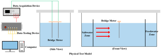
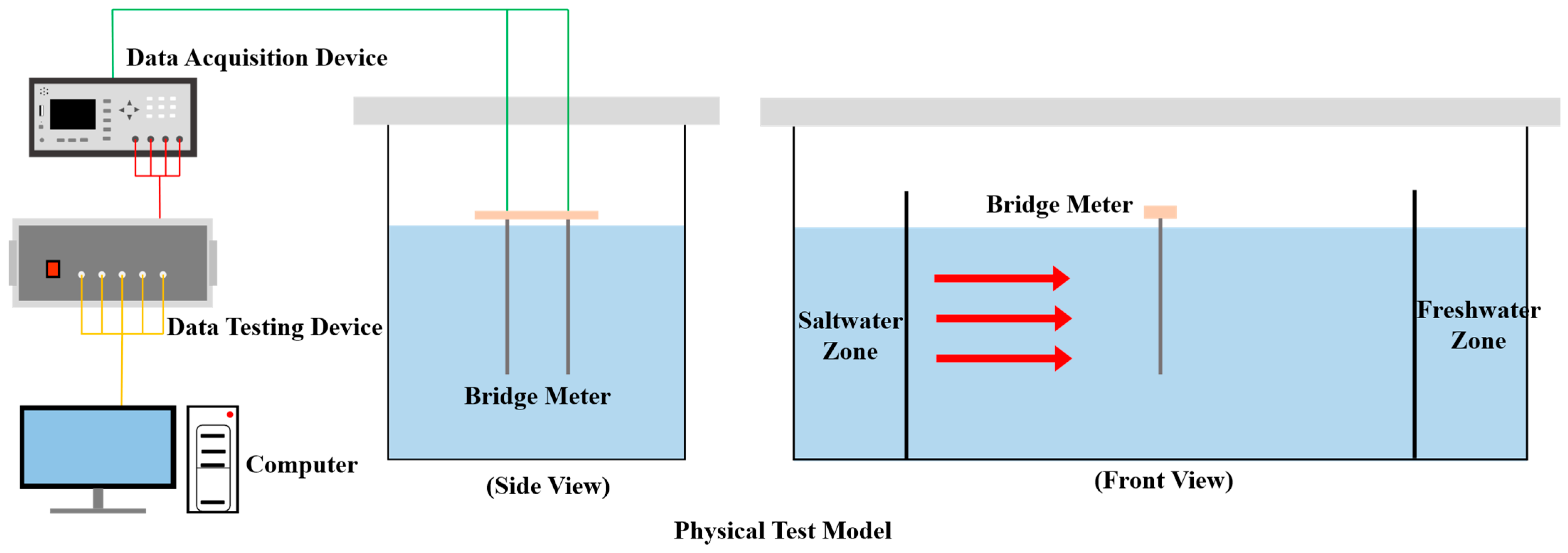
The test apparatus consists of two components: a physical test model and a data acquisition and measurement device. These components are shown in Figure 1 and described in detail below.

Figure 1. Schematic diagram of the experimental setup.

2.1.1. Physical Test Model

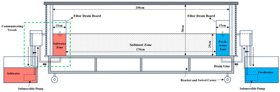
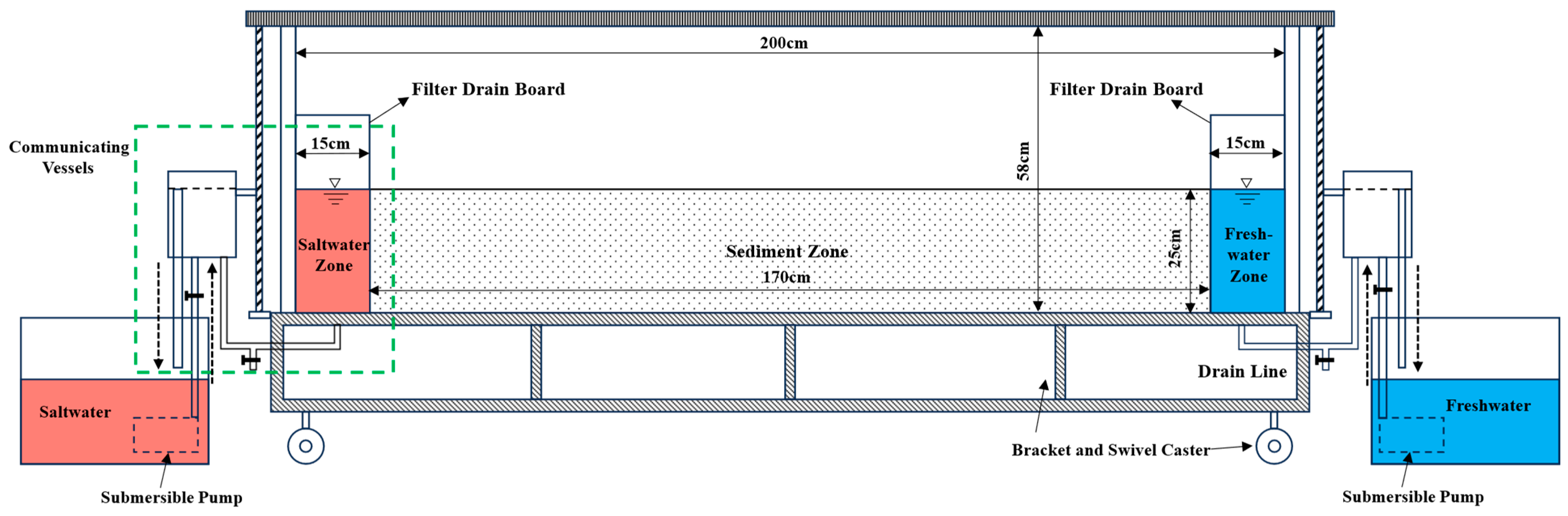
This physical model apparatus is a water tank constructed from 2 -cm -thick transparent acrylic sheets, measuring 200 cm in length, 50 cm in width, and 58 cm in height. It is divided into three sections: a freshwater chamber, a saltwater chamber, and a medium chamber (Figure 2). The medium chamber spans 170 cm in length, while the freshwater and saltwater chambers on its left and right sides each measure 15 cm. Filter plates made of geogrid and 100-mesh filter cloth separate the water chamber from the medium chamber. This design ensures good hydraulic connectivity while preventing sediment from entering the adjacent water chambers. Each water chamber is equipped with inlet and outlet pipes connected to communicating vessels, which control the freshwater and saltwater head boundaries. Both systems operate as self-circulating units, allowing for the reuse of water resources. The inlet pipes for the freshwater and saltwater chambers connect to tanks supplied by submersible pumps to replenish the aquifer. Drainage pipes at the bottom of both chambers allow for freshwater removal during the initial phases.

Figure 2. Schematic diagram of physical test model.

To enable real-time recording of the brackish-freshwater interface during seawater intrusion, calibrated paper is attached to the midpoint of the outer wall of the medium chamber, as well as to both sides of the freshwater and brackish-water chambers. The entire outer edge of the water tank is reinforced with sheet metal to ensure stability and prevent deformation. Because the tank becomes heavy when filled with sediment, it is mounted on a test stand with swivel casters, allowing easy movement during or after or subsequent relocation.

2.1.2. Data Acquisition and Measurement Device

Hardware Components

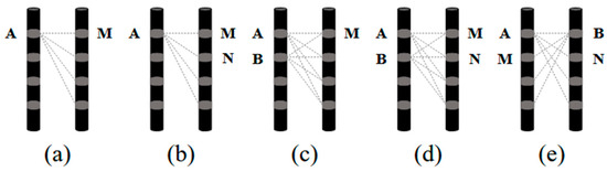
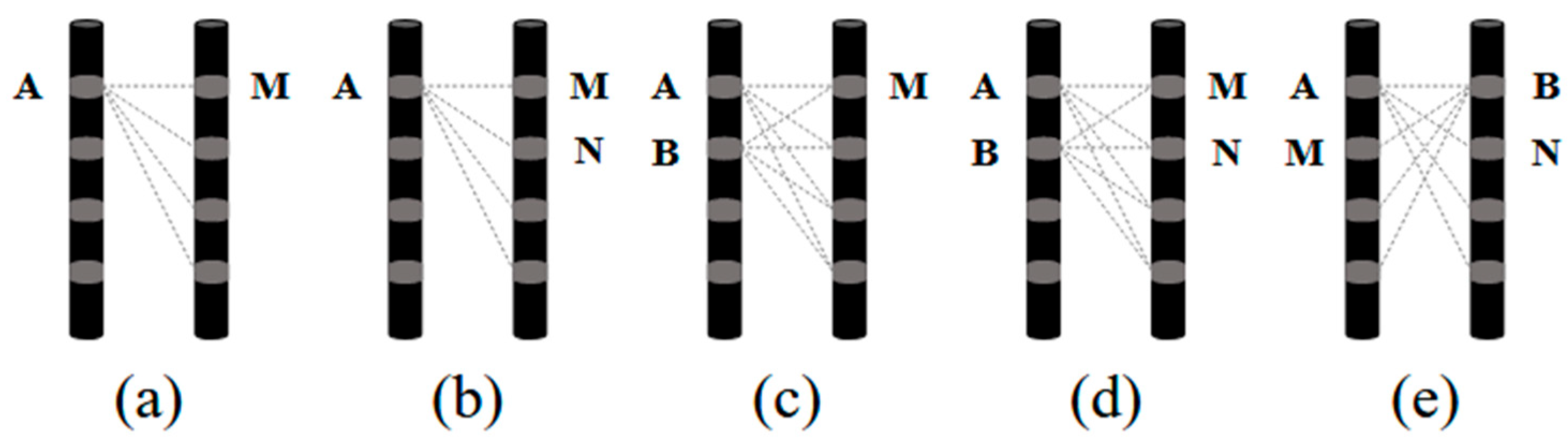
The resistivity imaging monitoring module consists of an array electrode system and a data acquisition device, with the array electrode system serving as the core component. The data acquisition method within this system is equally important: different acquisition configurations produce varying data quality, sensitivity to subsurface features, and imaging resolution. Common data acquisition methods include single-pole-single-pole (A-M) (Figure 3a), single-pole-dipole (A-MN, AB-M) (Figure 3b,c), and dipole-dipole (AB-MN, AM-BN) (Figure 3d,e). Here, A and B denote current injection dipoles, and M and N denote potential measurement dipoles. Numerical simulations conducted for this study found that the dipole-dipole configuration yields high-quality data. Therefore, the dipole-dipole arrangement was selected for all experiments in this study.

Figure 3. Data acquisition method (a) single-pole–single-pole; (b,c) single-pole–dipole; (d,e) dipole–dipole.

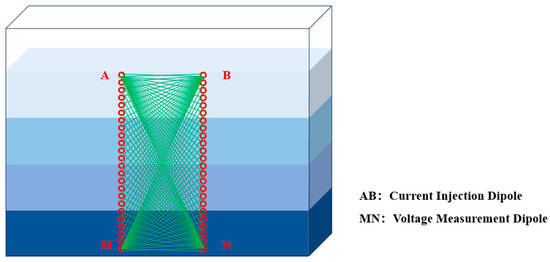
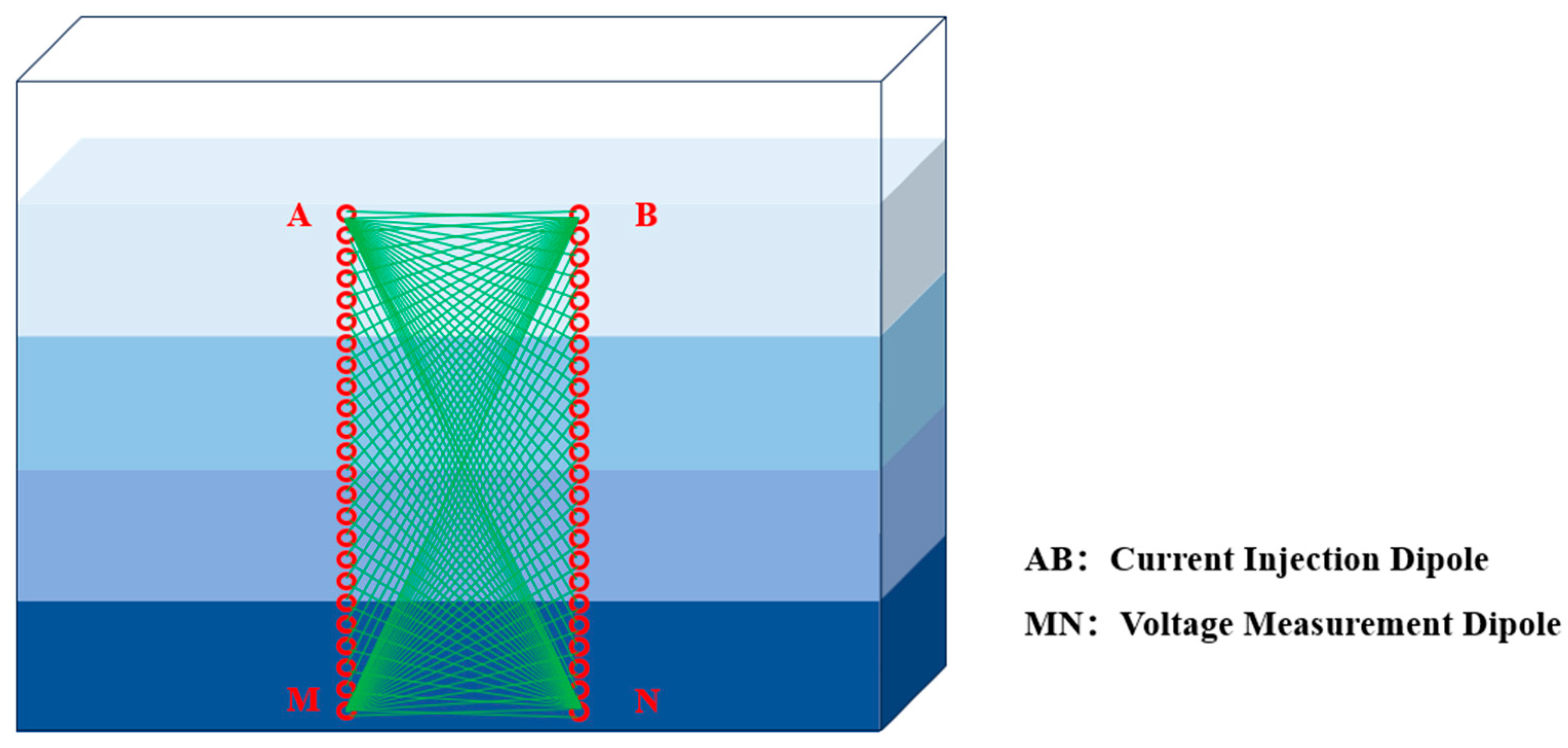
The electrode layout affects the resolution of resistivity imaging. A dual vertical electrode array configuration is employed in this experiment, where each array comprises 24 electrodes. Compared with previous layouts, this configuration provides greater flexibility and allows for the deployment of multiple arrays for three-dimensional imaging. The data acquisition process, current injection electrodes and voltage measurement electrodes are alternated horizontally and then moved downward layer by layer. As shown in Figure 4, the dots represent current injection and voltage measurement electrodes. Electrodes A and B inject current, while M and N measure voltage. A fixed pair of A-B electrodes injects current while voltage electrodes alternate left and right and move downward. After completing the voltage measurements, the current electrodes move to the next position, and the process repeats. If an array has n electrodes, one current dipole pair corresponds to (n-3) voltage measurements. Therefore, n electrodes can produce n × (n-3) data points. In this experiment, 48 electrodes produced 48 × 45 = 2160 data points.

Figure 4. Schematic diagram of array electrode layout and data acquisition method.

The data acquisition system includes a control box and a bridge instrument. The control box contains multiple multi-channel relay modules, each capable of connecting to 16 electrodes. The experiment uses the Amber AT281x bridge instrument, controlled by a 32-bit ARM microprocessor(Changzhou Anbai Instrument Company of China) and equipped with an RS232 interface for communication with a computer.

Software Components

This testing software comprises resistance acquisition software and resistivity imaging software. The acquisition software controls the relay output modules to switch circuit connections, allowing each electrode to act as either an injection or measurement electrode. The user presets parameters such as the number of acquisitions and stabilization duration, enabling automated operation. Upon completion, data are saved automatically to a specified directory. The resistivity imaging software includes six main components: data management, data preprocessing, parameter configuration, measurement curve display, resistivity image display, and image information. The data management component handles loading and saving of measured and processed resistivity distribution data. Data preprocessing removes anomalous data points caused by environmental noise or interference based on user-defined upper and lower limits; the parameter settings include residual thresholds, regularization parameters, and iteration counts, with default values of 1 × 10⁻⁵, 0.01, and 3, respectively. These parameters are adjusted to enhance imaging resolution and inversion convergence speed, and can be modified as needed. The measurement curve display automatically visualizes the loaded data, while the resistivity image display provides an intuitive visualization of resistivity distributions. Image information is used to adjust color scales, save imagery, and calculate the average resistivity of a profile.

2.2. Test Materials

2.2.1. Water Samples

The freshwater chamber uses tap water, while the saltwater chamber contains a prepared NaCl solution simulating seawater. Although natural seawater contains complex ionic compositions, NaCl accounts for approximately 90% of dissolved salts. Thus, NaCl solutions with equivalent concentrations exhibit similar resistivity properties to seawater. Based on prior seawater intrusion studies, a saltwater solution was used for convenience.

A 3.5% NaCl solution (density of 1.025 g/cm³) was prepared. To visually observe the brackish-saltwater interface during intrusion, Carmine Red dye (1-(4-sulfonic acid-1-naphthylazo)-2-hydroxy-6,8-naphthalenedisulfonic acid trisodium salt) was added at 0.75 g/L. This tracer is brightly colored, highly soluble, environmentally safe, and does not chemically interact with the saltwater, making it well-suited for indoor visualization of seawater intrusion.

2.2.2. Sediment Samples

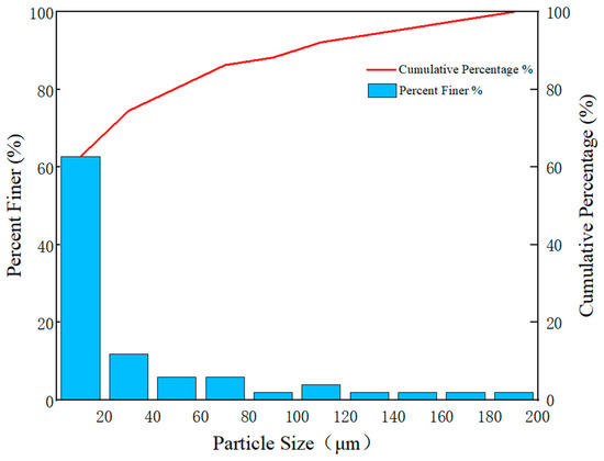
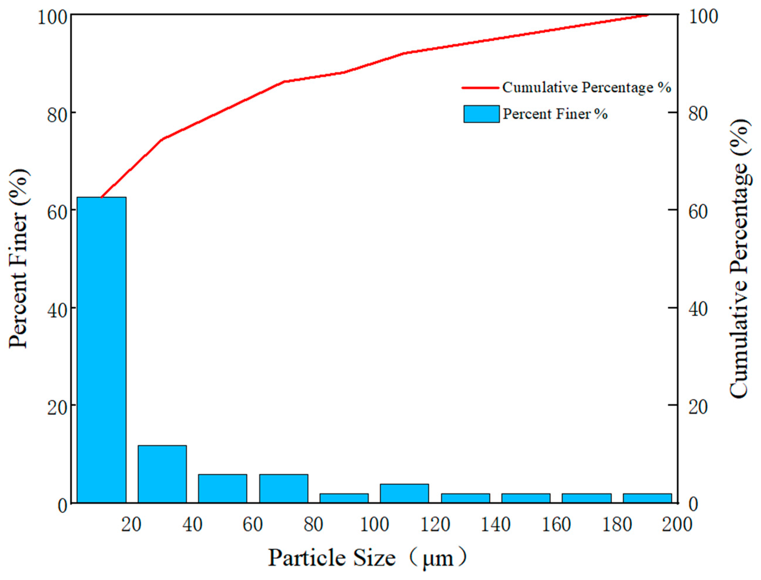
The porous medium used in this test has a particle size range of 0.02–0.2 mm. The grain-size distribution is shown in Figure 5.

Figure 5. Gradation distribution chart of porous media.

2.2.3. Measurement Electrode

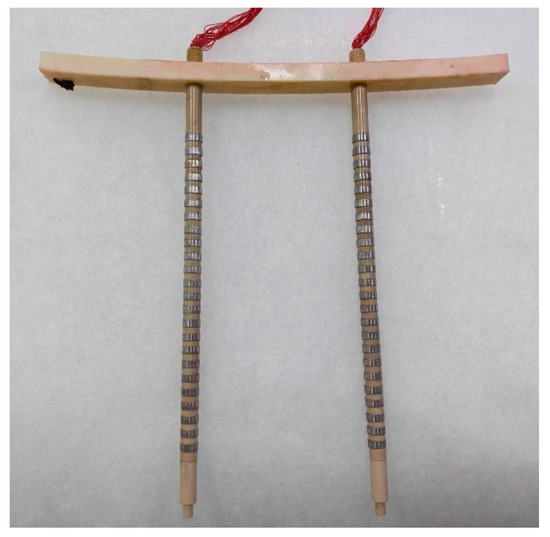
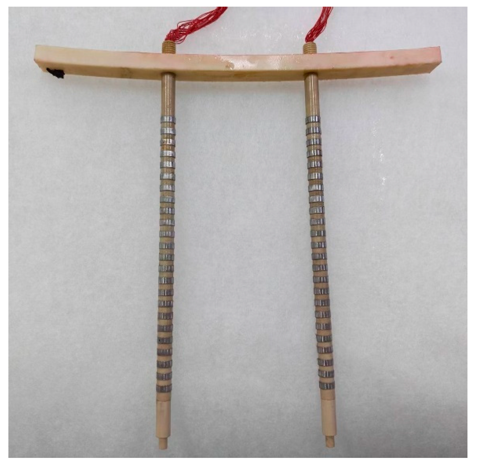
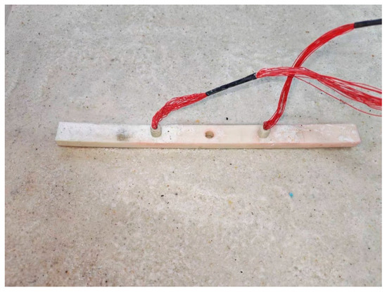
The experiment uses the Amber AT281x bridge instrument equipped with 48 electrodes evenly distributed on both sides of the device. The spacing between electrode systems is 100 mm, and the spacing between individual electrodes is 6 mm. The physical configuration is shown in Figure 6.

Figure 6. Schematic diagram of the measurement electrode assembly.

2.3. Testing Procedure

(1)

Sufficient quantities of porous medium were loaded into the water tank to create a homogeneous submerged aquifer, and the sand body was compacted after every 4 cm of sediment to ensure uniform sample distribution until the sand layer reached a thickness of 25 cm. To ensure good electrical coupling between the electrodes and the sand layer, the bridge instrument was buried in the center of the medium chamber during the test. Sand was then added layer by layer until all electrodes were completely buried. The surrounding sand layer was gently compacted with a small hammer. The electrodes within the borehole were embedded on both sides of the sand layer, ensuring that all electrodes were in close contact with the sand layer, as shown in Figure 7.

Figure 7. Electrode implantation.

(2)

The water heads of the freshwater and brine chambers were adjusted to 25 cm. A continuous supply of freshwater was maintained at a low flow rate to prevent introducing excessive gas into the aquifer.

(3)

As the water level in the freshwater chamber rises, freshwater permeates through the filter plate into the medium chamber. The area of porous medium saturated by freshwater gradually expanded within the medium chamber, and freshwater permeates through the filter plate into the brine chamber.

(4)

After the brine chamber water level rose to 25 cm and a constant flow of freshwater emerged from the communicating vessel on the brine chamber side, the entire aquifer was saturated with freshwater. The water supply was stopped, and the system was allowed to settle for measurement.

(5)

Constant water levels of 25 cm were maintained in both the freshwater and brine chambers. A water-blocking baffle was temporarily installed in the brine chamber to prevent freshwater from flowing into it. The drain outlet at the bottom of the brine chamber was opened to rapidly discharge its freshwater contents, after which the outlet was immediately closed. The chamber was refilled with brine to 25 cm, the baffle removed, and the seawater intrusion test formally commenced.

(6)

Brine was continuously supplied at a constant flow rate to maintain a stable brine density in the brine chamber. Resistivity imaging was used to monitor seawater migration in real time. Monitoring personnel closely observed the test system to ensure proper monitoring operations, maintain accurate data records, and document any test anomalies for subsequent data processing.

(7)

The test concluded when the seawater wedge showed no significant change in migration distance over a two-day period.

2.4. Electrical Resistivity Tomography

Cross-hole ERT captures the resistivity distribution of the medium within a target area by measuring the potential or potential difference generated by an electric field from a direct current point source at various locations around the target area. Most hydrogeological electromagnetic systems adopt quasi-static physics and conductive current rather than wave propagation. Electromagnetic tomography is an exception, using linearly propagating high-frequency waves like seismic tomography; in contrast, ERT current flows along minimum-resistivity paths based on conductive field rules [28,29,30]. Consequently, ray theory cannot be applied, necessitating alternative processing methods. The key challenge in cross-hole ERT lies in the reconstruction algorithm, which directly impacts imaging speed and quality, leading to continued research on reconstruction techniques. Since the observed field is a stable nonlinear potential field, the imaging problem must be linearized, similarly to other nonlinear problems, followed by iterative model refinement. Forward algorithms are typically nonlinear, while inversion algorithms predominantly remain based on linear iteration. However, several nonlinear algorithms have also been developed in recent years.

The forward algorithm primarily relies on the fundamental differential equation of direct current methods (the Poisson equation) to derive the boundary value problem for a steady-state current field under laboratory conditions. The solution to this boundary value problem is transformed into a functional extremum problem solved by the finite element method through the variational approach. Here, we used the finite element method with the forward algorithm for cross-hole electrical resistivity imaging under laboratory conditions. The inverse algorithm, based on the least-squares method, constructs an objective function that combines both model and data constraints. Minimizing this objective function using the Gauss-Newton iterative algorithm facilitates the inverse algorithm for cross-hole electrical resistivity imaging.

2.4.1. Forward Modeling Principle of Cross-Hole Electrical Resistivity Imaging

The forward problem in cross-hole electrical resistivity imaging involves determining the response characteristics of the cross-hole electrical potential based on known resistivity and field source distributions. In practice, observing and analyzing artificially generated geoelectric field patterns helps identify targets or resolve geological problems. Common forward numerical simulation methods include the integral equation approach [31], boundary element method [32], finite difference method [33], and finite element method [34], with the latter two being widely used to solve geoelectric field problems. Because the finite difference method is less suitable for complex spatial geometries, the finite element method, which is an approximation technique based on variational principles and the weighted residual method, is well-suited for complex and variable geophysical problems. With advancements in computational power, the finite element method has gained increasingly widespread application in geophysics [35,36].

Steady Electric Field Flow and Boundary Value Problems

Cross-hole electrical resistivity imaging evolved from ground-based direct current (DC) resistivity surveying. Unlike surface-based DC methods, electrodes for both excitation and measurement are deployed within boreholes. Using direct current, this technique calculates potential responses through the analysis of steady-state electric fields.

For isotropic media, the continuity equation for current density and charge density can be derived from the law of charge conservation:

$$\nabla \cdot \stackrel{\rightharpoonup }{J}=-{\displaystyle \frac{\partial \mathrm{q}}{\partial \mathrm{t}}}$$

(1)

where q represents the charge distribution density.

For two-dimensional problems, if a point charge e is located at $r_A=(x_A,y_A)$, the charge density can be expressed using the Dirichlet functions:

$$\mathrm{q}=\mathrm{e}\delta (r-r_A)=e\delta (x-x_A)\delta (y-y_A)$$

(2)

The definition of current intensity is:

$$I=-{\displaystyle \frac{\partial e}{\partial t}}$$

(3)

To establish a relationship between the potential function u and the current intensity I, we utilize the properties of the function δ to derive the differential equation satisfied by a point source:

$${\displaystyle \frac{\partial }{\partial x}}\left({\displaystyle \frac{1}{\rho }}{\displaystyle \frac{\partial u}{\partial x}}\right)+{\displaystyle \frac{\partial }{\partial y}}\left({\displaystyle \frac{1}{\rho }}{\displaystyle \frac{\partial u}{\partial y}}\right)=-I\delta (r-r_A)\hspace{1em}(x,y),(x_A,y_A)\in \Omega$$

(4)

From the continuity of potential, it follows that at the interface:

$$u_1=u_2$$

(5)

From the continuity of the tangential component of the current density, it follows that at the interface:

$${\displaystyle \frac{1}{{\rho }_1}}{\displaystyle \frac{\partial u_1}{\partial n}}={\displaystyle \frac{1}{{\rho }_2}}{\displaystyle \frac{\partial u_2}{\partial n}}$$

(6)

Here, n denotes the direction of the normal vector at the interface. For any stable current field, the potential distribution function satisfies Equations (4)–(6) above.

To obtain an accurate electric field distribution that uniquely determines the solution to the differential equation, corresponding boundary conditions must be specified that define the constraints that must be satisfied at the boundaries of the study region. Potential functions typically satisfy three types of boundary conditions:

First-order boundary conditions (Dirichlet boundary conditions):

$$u(x,y){|}_{\partial \Omega }=\phi (x,y)$$

(7)

Second-type boundary conditions (Neumann boundary conditions):

$${\displaystyle \frac{\partial u(x,y)}{\partial n}}{|}_{\partial \Omega }=\phi (x,y)$$

(8)

Third-type boundary conditions (mixed boundary conditions):

$$\left({\displaystyle \frac{\partial u(x,y)}{\partial n}}+\alpha u(x,y)\right){|}_{\partial \Omega }=\phi (x,y)$$

(9)

Here, ∂Ω denotes the boundary of the study region, and φ(x, y) represents the known boundary function values. By combining Equation (4) with the boundary conditions, we obtain a two-dimensional point-source boundary-value problem, whose solution corresponds to solving the forward problem.

Finite Element Solution

While boundary value problems can be solved analytically for simple models, solutions to complex models require numerical simulation. The finite element method is a common approach for solving forward electric field problems, capable of flexibly representing any model. The solution process involves constructing the variational problem, mesh partitioning, linear interpolation, element analysis, and overall synthesis.

(1)

Variational problem

Based on the equations and boundary conditions for a steady-state current field, the boundary value problem for a two-dimensional constant field is as follows:

$$\left\{\begin{array}{l}\nabla \cdot \left({\displaystyle \frac{1}{\rho }}\nabla u\right)=-I\delta (r-r_A)\hfill \\ \left({\displaystyle \frac{\partial u}{\partial n}}+\alpha u\right){|}_{\partial \Omega }=\phi \hfill \end{array}\right.$$

(10)

when the electric flux at the boundary equals zero, α = 0, which corresponds to Neumann boundary conditions; when the value at the boundary is infinity, $\alpha =n\cdot r/{\left|r\right|}^2$, which corresponds to mixed boundary conditions. Due to laboratory space constraints and experimental apparatus design, Neumann boundary conditions are appropriate for forward calculations under laboratory conditions.

In the finite element method, the boundary value problem (10) must be transformed into a variational problem.

Where n represents the outer normal vector of Ω. Based on the boundary conditions in Equation (9), we obtain:

$$\begin{array}{c}I(u)={\displaystyle {\iint }_{\Omega }\frac{1}{\rho }}{(\nabla u)}^2-I\delta (r-r_A)ud\Omega -{\displaystyle {\oint }_{\partial \Omega }\frac{1}{\rho }}\stackrel{\rightharpoonup }{J}\cdot \stackrel{\rightharpoonup }{n}uds+{\displaystyle {\oint }_{\partial \Omega }\frac{1}{\rho }\alpha u^{2}ds}\\ \delta I(u)=0\end{array}$$

(11)

(2)

Grid Partitioning

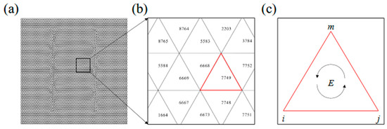
Solving variational problems using the finite element method requires the study region to be divided into numerous discrete elements, which may be triangular, rectangular, tetrahedral, or cubic. For the two-dimensional problem, this study employed a triangular mesh that subdivided the study region into 9024 equilateral triangles, as shown in Figure 8.

Figure 8. Finite element mesh partitioning: (a) Grid partitioning diagram of the entire study area; (b) grid partitioning diagram of the local study area; (c) single grid diagram.

The triangular units can be identified by a sequential numbering scheme, where individual units are designated as $E_{k\prime }(k=1,2,3,\dots ,NE)$ and NE represents the total number of triangular units. Similarly, another set of integers can be used to encode and identify nodes at the vertices of each triangular unit, denoted as Pi, where $(x_i,y_i), (i=1,2,3,\dots ,NP)$ represents the coordinates, and NP denotes the total number of nodes. Since each triangular unit is associated with multiple nodes, it is also necessary to assign integer codes to each node position within a given triangular unit, which is referred to as local encoding.

(3)

Linear interpolation

For each triangular cell E, the three nodes are labeled moving counterclockwise as i, j, and m, with coordinates (x_i, y_i), (x_j, y_j), and (x_m, y_m), respectively. The corresponding potential function values for these nodes are u = [u_i, u_j, u_m].

In gridded regions, the potential distribution across the entire continuous space can be approximated by solving for the function values at a finite number of undetermined nodes within the study area. For a sufficiently fine triangular element mesh, it can be assumed that the potential within each triangular element E varies linearly with the coordinates. Within each triangular element, the potential function u can be expressed as:

$$u=ax+by+c$$

(12)

where the coefficients a, b, and c can be determined using the function values and coordinates at the element nodes, employing the method of undetermined coefficients. For a triangular element E, the function values satisfy:

$$\begin{array}{l}{\mathrm{u}}_{\mathrm{i}}{(\mathrm{x}}_{\mathrm{i}}{,\mathrm{y}}_{\mathrm{i}}{)=\mathrm{ax}}_{\mathrm{i}}{+\mathrm{by}}_{\mathrm{i}}+\mathrm{c}\\ {\mathrm{u}}_{\mathrm{j}}{(\mathrm{x}}_{\mathrm{j}}{,\mathrm{y}}_{\mathrm{j}}{)=\mathrm{ax}}_{\mathrm{j}}{+\mathrm{by}}_{\mathrm{j}}+\mathrm{c}\\ {\mathrm{u}}_{\mathrm{m}}{(\mathrm{x}}_{\mathrm{m}}{,\mathrm{y}}_{\mathrm{m}}{)=\mathrm{ax}}_{\mathrm{m}}{+\mathrm{by}}_{\mathrm{m}}+\mathrm{c}\end{array}$$

(13)

where N_i, N_j, and N_m are referred to as shape functions, also known as linear interpolation basis functions on the triangular element E, and are expressed respectively as:

$$\left\{\begin{array}{l}{N}_i={\displaystyle \frac{1}{2{\Delta }_E}}(a_{i}x+b_{i}y+c_i)\\ N_j={\displaystyle \frac{1}{2{\Delta }_E}}\left(a_{j}x+b_{j}y+c_j\right)\\ N_m={\displaystyle \frac{1}{2{\Delta }_E}}(a_{m}x+b_{m}y+c_m)\end{array}\right.$$

(14)

(4)

Unit Analysis

After grid partitioning and linear interpolation, the integral over the study region is decomposed into integrals over each E, yielding:

$$I(u)={\displaystyle \sum _1^{NE}{\displaystyle {\iint }_{\Omega }\frac{1}{\rho }}}{(\nabla u)}^2-I\delta (r-r_A)ud\Omega -{\displaystyle {\oint }_{\partial \Omega }\frac{1}{\rho }}\stackrel{\rightharpoonup }{J}\cdot \overrightarrow{n}uds+{\displaystyle {\oint }_{\partial \Omega }\frac{1}{\rho }}\alpha u^{2}ds$$

(15)

Then, the functional within a triangular element E will be computed as:

$$I_E(u)={\displaystyle {\iint }_{\mathcal{E}}\frac{1}{{\rho }_E}}{(\nabla u)}^2-I\delta (r-r_A)ud\Omega -{\displaystyle {\oint }_{\partial \Omega }\frac{1}{{\rho }_E}}\overrightarrow{J}\cdot \overrightarrow{n}uds+{\displaystyle {\oint }_{\partial \Omega }\frac{1}{{\rho }_E}}\alpha u^{2}ds$$

(16)

where ρ_E represents the resistivity within the triangular element.

To compute the integral over each triangular element E, the gradient vector of the potential function on each triangular element must be determined as:

$$\nabla u={\left[\begin{array}{cc}{\displaystyle \frac{\partial u}{\partial x}}& {\displaystyle \frac{\partial u}{\partial y}}\end{array}\right]}^T=\left[\begin{array}{ccc}{\displaystyle \frac{\partial N_i}{\partial x}}& {\displaystyle \frac{\partial N_j}{\partial x}}& {\displaystyle \frac{\partial N_m}{\partial x}}\\ {\displaystyle \frac{\partial N_i}{\partial y}}& {\displaystyle \frac{\partial N_i}{\partial y}}& {\displaystyle \frac{\partial N_i}{\partial y}}\end{array}\right]={\displaystyle \frac{1}{2{\Delta }_E}}\left[\begin{array}{ccc}{a}_i& a_j& a_m\\ b_i& b_j& b_m\end{array}\right]={\displaystyle \frac{1}{2{\Delta }_E}}\overrightarrow{B}$$

(17)

From this, it is evident that ∇u depends solely on the node coordinates and the function values at the nodes, and remains constant within a triangular element.

Due to limitations in space and materials within the laboratory, infinite boundary conditions do not exist; therefore, the third and fourth terms of the integral are equal to zero.

(5)

Overall Synthesis

Summing across all triangular elements yields:

$$I(u)={\displaystyle \sum _1^{NE}{I}_E}(u)={\displaystyle \sum _1^{NE}{u}^T}{K}_{E}u+{\displaystyle \sum _1^{NE}{u}^T}{P}_E=u^{T}Ku+u^{T}P$$

(18)

Taking the variational derivative of Equation (18) and setting it equal to zero yields the following system of linear equations:

$$Ku=P$$

(19)

where K represents the stiffness matrix, and P denotes the load vector. Solving the above equation yields the displacement u at each node.

2.4.2. Principles of Well-Spaced Resistivity Imaging Inversion

Inversion is a fundamental type of problem in geophysical exploration [37]. The inversion problem in borehole resistivity imaging involves determining the subsurface resistivity distribution from known potential responses and field sources. Constraints arising from the physical environment, limited observational data, low measurement accuracy, and insufficient prior information contribute to making the solution computationally challenging and non-unique. Over time, numerous effective methods have emerged, including both iterative and non-iterative approaches [38]. Non-iterative techniques include linear back-projection, singular value decomposition, and Tikhonov regularization, while iterative methods include the conjugate gradient method, the Gauss-Newton method, and the Landweber method. A detailed exposition and implementation of the Gauss-Newton inversion method used in this study is provided below.

Objective Function Construction

The inverse problem for cross-hole electrical resistivity imaging can be expressed as:

$$d=G(m)+e$$

(20)

where m represents the vector of resistivity model parameters, d denotes the vector of measured potential data, e represents the vector of measurement errors, and G is the nonlinear forward model operator. G(m) describes the mapping relationship between model parameters and simulated data; i.e., how to derive simulated data from known model parameters.

The approach proposed by Tikhonov in 1997 uses an objective function for the cross-hole electrical resistivity imaging inverse problem that can be formulated as:

$$\Phi (m)={\Phi }_d(m)+\lambda {\Phi }_m(m)$$

(21)

where Φ(m) denotes the overall objective function; Φ_d(m) denotes the data objective function; Φ_m(m) denotes the model objective function; λ denotes the regularization parameter.

Assuming that the measurement errors follow a Gaussian distribution and are mutually independent, the objective function for the data can be expressed as the fitting error between the measured data and the theoretical data.

$${\Phi }_d(m)={\displaystyle \sum _{i=1}^N{\left(d_i-G_i(m)\right)}^2}$$

(22)

Substituting the data objective function and model objective function in matrix form into Equation (22) yields the matrix form of the total objective function:

$$\Phi (m)={\left(d-G(m)\right)}^T\left(d-G(m)\right)+{(Lm)}^T(Lm)$$

(23)

The Gauss-Newton Inversion Method

Newton’s method, an old inversion method with fast convergence, demands costly computation/storage of the Hessian matrix and its inverse. Moreover, the Hessian inverse may be ill-conditioned/singular, endangering convergence—leading to the Gauss-Newton method, an approximate Hessian inverse alternative.

To minimize the total objective function Φ(m), we differentiate Equation (23) with respect to the resistivity model parameter m and set the derivative equal to zero:

$${\displaystyle \frac{\partial \Phi (m)}{\partial m}}=-2J{(m)}^T\left(d-G(m)\right)+2\lambda L^{T}Lm=0$$

(24)

Here, J(m) represents the Jacobian matrix, also known as the partial derivative matrix or sensitivity matrix, which denotes the partial derivatives of the forward model function G(m) with respect to the resistivity model parameters m, expressed as:

$$J(m)={\displaystyle \frac{\partial G(m)}{\partial m}}$$

(25)

To avoid computing the second-order partial derivatives of the forward model function G(m), the operator G is linearized using the Taylor series.

$$G(m+\delta m)=G(m)+J(m)\delta m+o(\delta m^2)$$

(26)

By neglecting higher-order terms in the Taylor series expansion and combining Equations (24) and (26), the Gaussian-Newton iteration formula for the k-th step is obtained as:

$$(J{(m_k)}^{T}J(m_k)+\lambda L^{T}L)\delta m=J{(m_k)}^T\left(d-G(m_k)\right)-\lambda L^{T}L{m}_k$$

(27)

Once the correction factor δ_m for the resistivity model is determined using Equation (27), the new resistivity model m_k+1 is given by the following equation:

$$m_{k+1}=m_k+\alpha \delta m$$

(28)

Here, m_k+1 represents the new model, and α is the linear search parameter. Linear search is employed to control the magnitude of the resistivity correction. Typically, the Armijo criterion is used to select an appropriate step size α that provides a sufficient decrease in the objective function Φ(m). The iterative process continues until the objective function Φ(m) decreases to a specified value.

Partial Derivative Matrix Solver

Another essential step in solving the inverse problem is calculating the partial derivative matrix (Jacobian matrix) of the potential response (or apparent resistivity) with respect to the resistivity model parameters. The size, number, and dimensions of the finite element mesh directly impact the efficiency of the partial derivative computation, which affects the convergence rate of the solution. Common methods include the standard method, the differential method, the compensation circuit method, the Green’s function method, the perturbation method, and the exchange theorem, among others. This study adopts the standard method proposed by Yorkey et al [39]. to solve the partial derivative matrix.

Performing forward calculations using the finite element method yields:

$$Ku=P$$

(29)

where the load vector P is independent of the distribution of the resistivity model parameter m. Differentiating both sides of Equation (29) with respect to m and setting it equal to zero yields:

$${\displaystyle \frac{\partial Ku}{\partial m}}={\displaystyle \frac{\partial K}{\partial m}}u+K{\displaystyle \frac{\partial u}{\partial m}}=0$$

(30)

Thus, we can obtain

$${\displaystyle \frac{\partial u}{\partial m}}=-K^{-1}{\displaystyle \frac{\partial K}{\partial m}}u$$

(31)

All parameters in Equation (31) can be obtained through forward modeling, which confers the advantages of clear physical meaning and high precision for this method.

Smoothness Matrix Solver

To address the ill-posed nature of well-spaced resistivity imaging, model constraints are introduced into the objective function Φ(m). In the absence of prior information, model smoothing constraints are typically adopted, where adjacent resistivity model parameters exhibit smooth transitions and are weighted by the distance between grid points. For the k-th resistivity model parameter, the smoothing constraint is defined as:

$$R=\left({\displaystyle \frac{\delta m_k^1}{l^1}}+{\displaystyle \frac{\delta m_k^2}{l^2}}+{\displaystyle \frac{\delta m_k^3}{l^3}}-{\displaystyle \frac{\delta m_k}{l^1}}+{\displaystyle \frac{\delta m_k}{l^2}}+{\displaystyle \frac{\delta m_k}{l^3}}\right)/3$$

(32)

In the equation, $\delta m_k$ represents the correction factor for the resistivity model parameter of the kth grid, $\delta m_k^1 \delta m_k^2 \delta m_k^3$ denotes the correction factors for the resistivity model parameters of the three grids adjacent to the k-th grid, and $l^1 l^2 l^3$ indicates the distances from the center of the k-th grid to the centers of the three adjacent grids. Thus, the smoothing constraint for the entire resistivity model can be expressed in matrix form as:

$$R=L\delta m$$

(33)

where L denotes the smoothing model constraint matrix in Equation (33).

When two grids are adjacent:

$$L(i,j)={\displaystyle \frac{1}{l_{ij}}}$$

(34)

When two grids are not adjacent:

$$L(i,j)=0$$

(35)

In the formula, $l_{ij}$ represents the center-to-center distance between adjacent grid cells.

2.4.3. Model Method Verification

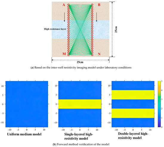
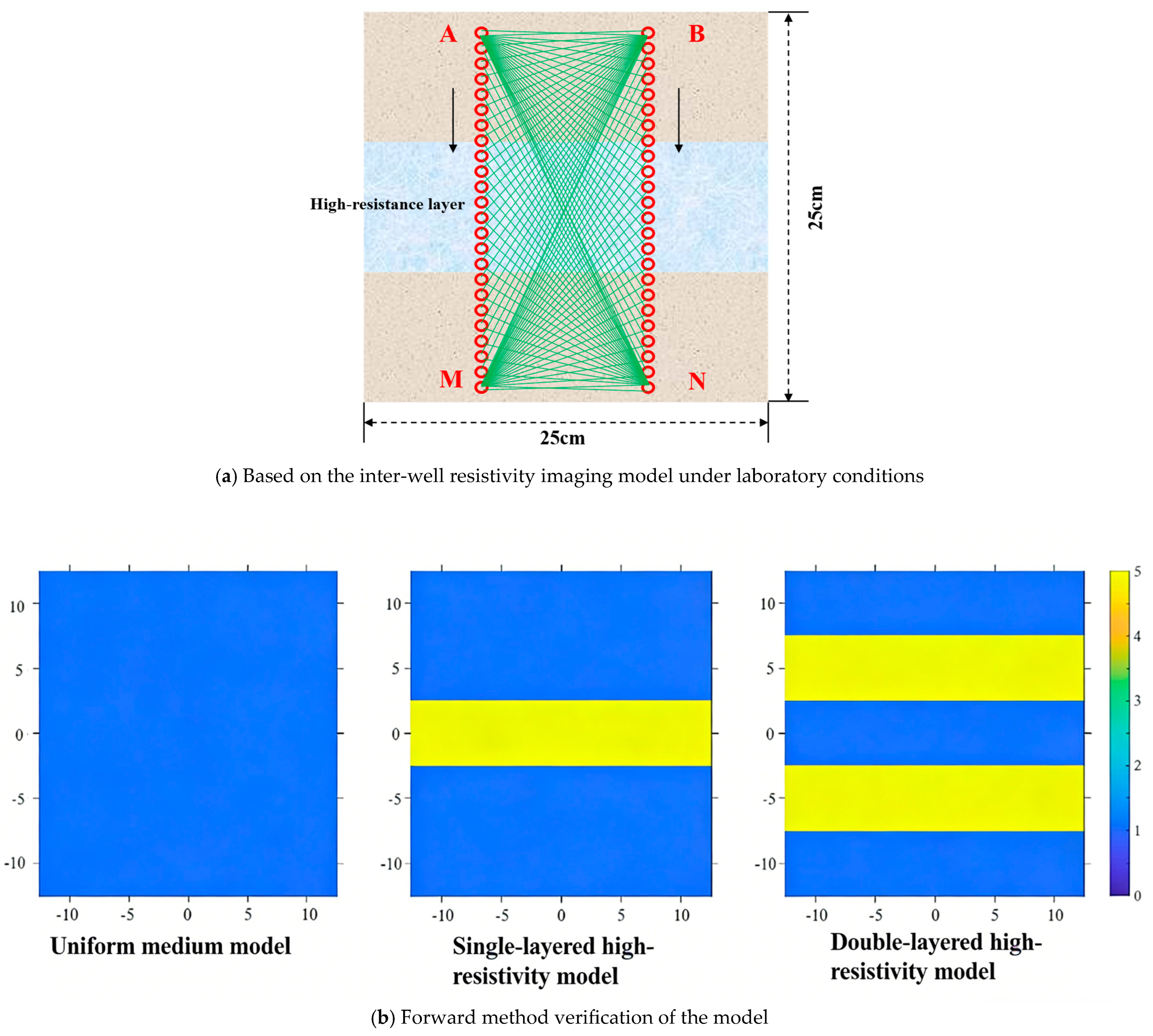
Within a square study area with a side length of 25 cm, an electrode array consisting of 48 point current sources was deployed, which was divided into two groups of 24. The inter-group distance was 10 cm, and the interval between adjacent point current sources was 0.8 cm (Figure 9a). Due to the constraints of laboratory space, the boundary condition was set as an insulating boundary condition. Subsequently, current was supplied to the two uppermost point current sources (designated as A and B), while the potentials were measured at all other point current sources. Three resistivity models were designed, namely a homogeneous medium model, a single-layered high-resistivity model, and a double-layered high-resistivity model. The resistivity of the layered high-resistivity zones was set to 5 Ω·m, and the background resistivity was set to 1 Ω·m (Figure 9b).

Figure 9. Verification of the model based on the inter-well resistivity imaging model and forward modeling method under laboratory conditions.

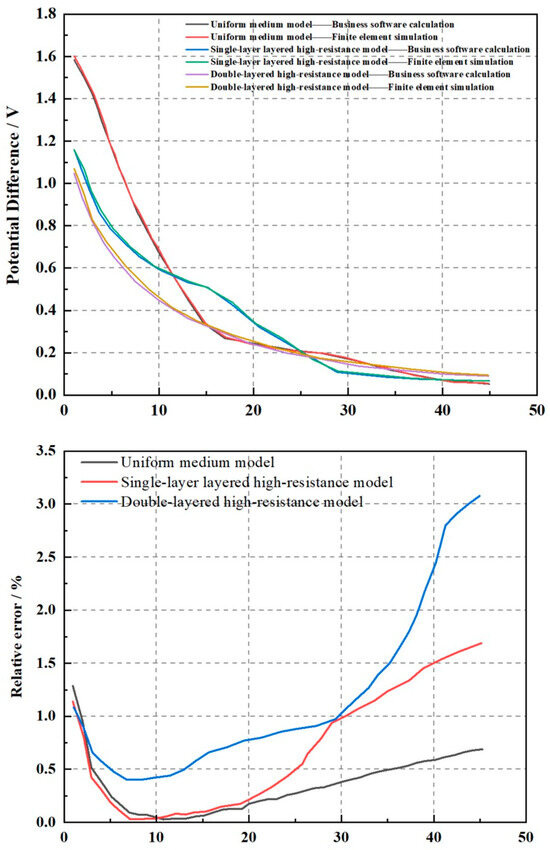
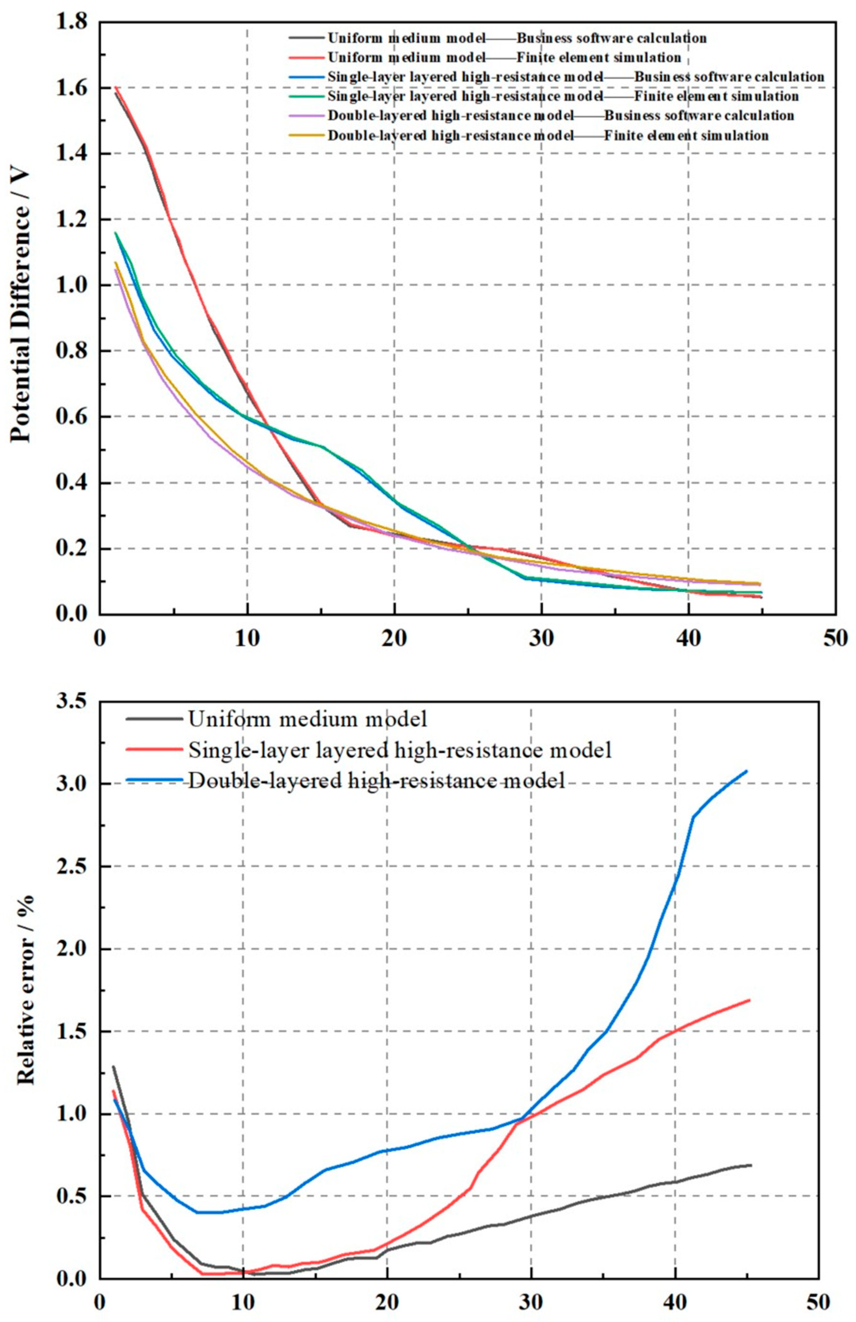
The three resistivity models above were calculated using commercial software and the finite element method described in this paper to obtain potential difference response curves respective to each model (Figure 10). Visually, the potential difference curves of the two methods almost completely overlap, indicating the reliability of the finite element method under laboratory conditions. Quantitative analysis via the calculation of their relative errors shows that all errors are less than 3.50%, and it was also found that the more complex the model, the larger the relative error (Figure 10). This further validates the correctness of the potential difference response curves obtained by the proposed method.

Figure 10. Finite element calculation simulation of formation resistivity imaging and comparison with commercial software calculation, as well as error analysis.

3. Results

The seawater intrusion test began at 23:00 on 11 September 2025 and ended at 23:00 on 26 September 2025, spanning approximately 360 h. During this period, 360 ERT monitoring sessions were conducted. Due to space constraints, the following analysis focuses on seawater intrusion migration patterns under zero-head-difference conditions. Fifteen representative time points were selected for inversion analysis (as shown in Table 1).

Table 1. ERT data monitoring schedule at zero head difference.

No.	Measure Time	Accumulate Intrusion Time(h)	Average Resistivity (Ω·m)
1	11 September 2025-24:00	1	56.83
2	12 September 2025-14:00	15	33.65
3	12 September 2025-23:00	24	30.93
4	13 September 2025-14:00	39	28.22
5	13 September 2025-23:00	48	25.34
6	14 September 2025-17:00	66	16.85
7	15 September 2025-17:00	90	11.44
8	16 September 2025-15:00	112	8.41
9	17 September 2025-19:00	140	6.24
10	19 September 2025-19:00	188	4.41
11	21 September 2025-23:00	240	3.85
12	23 September 2025-05:00	270	2.73
13	24 September 2025-11:00	300	2.52
14	25 September 2025-17:00	330	2.12
15	26 September 2025-23:00	360	1.14

3.1. Changes in the Seawater Intrusion Front

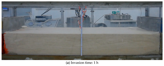
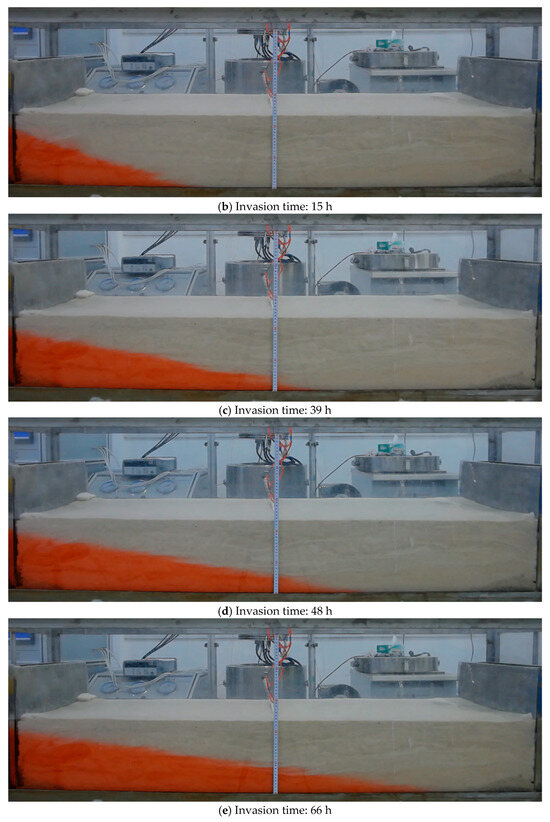
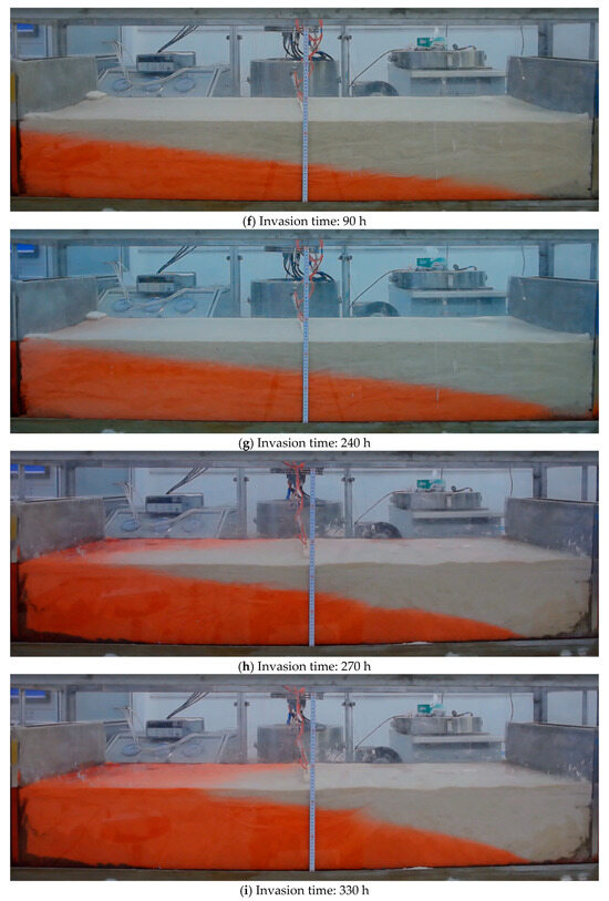
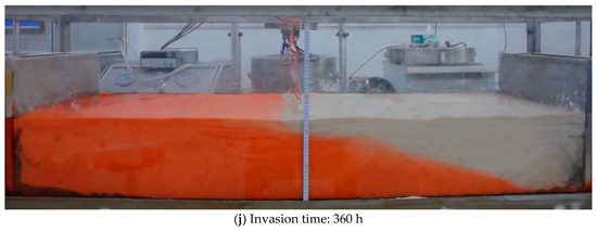
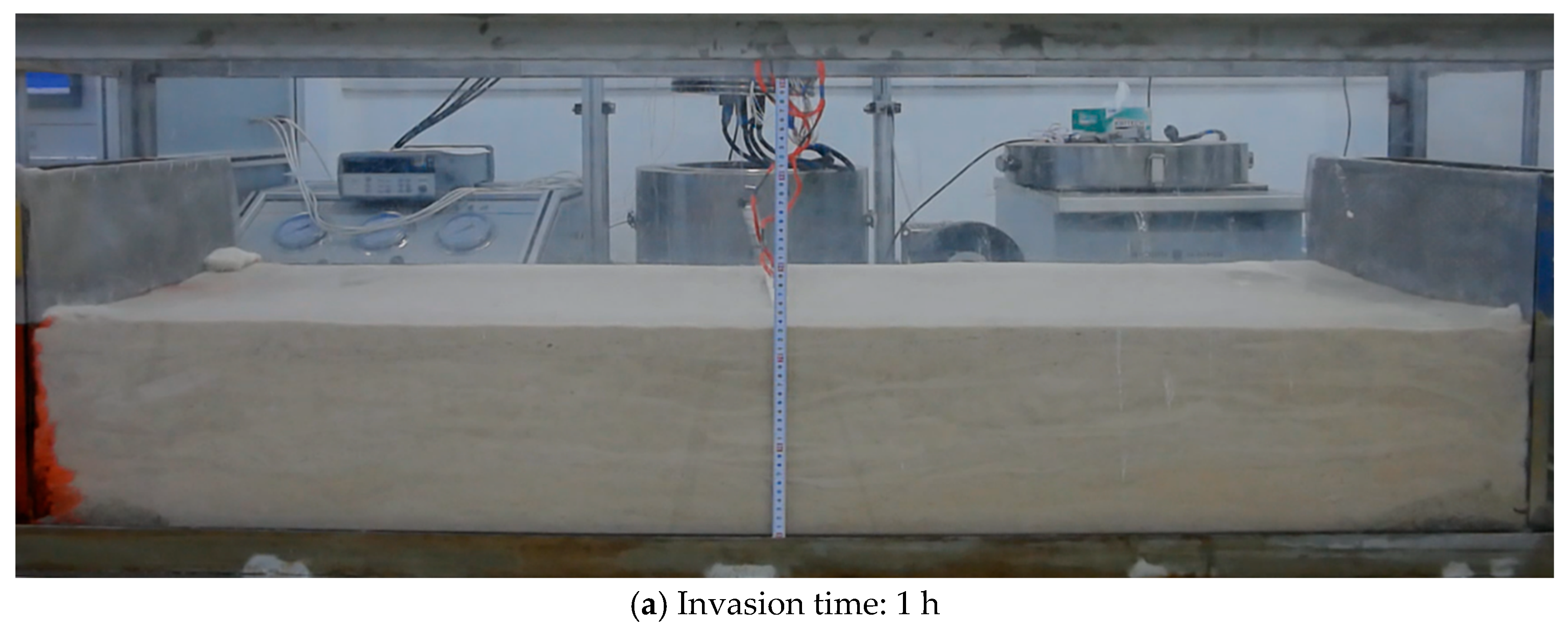
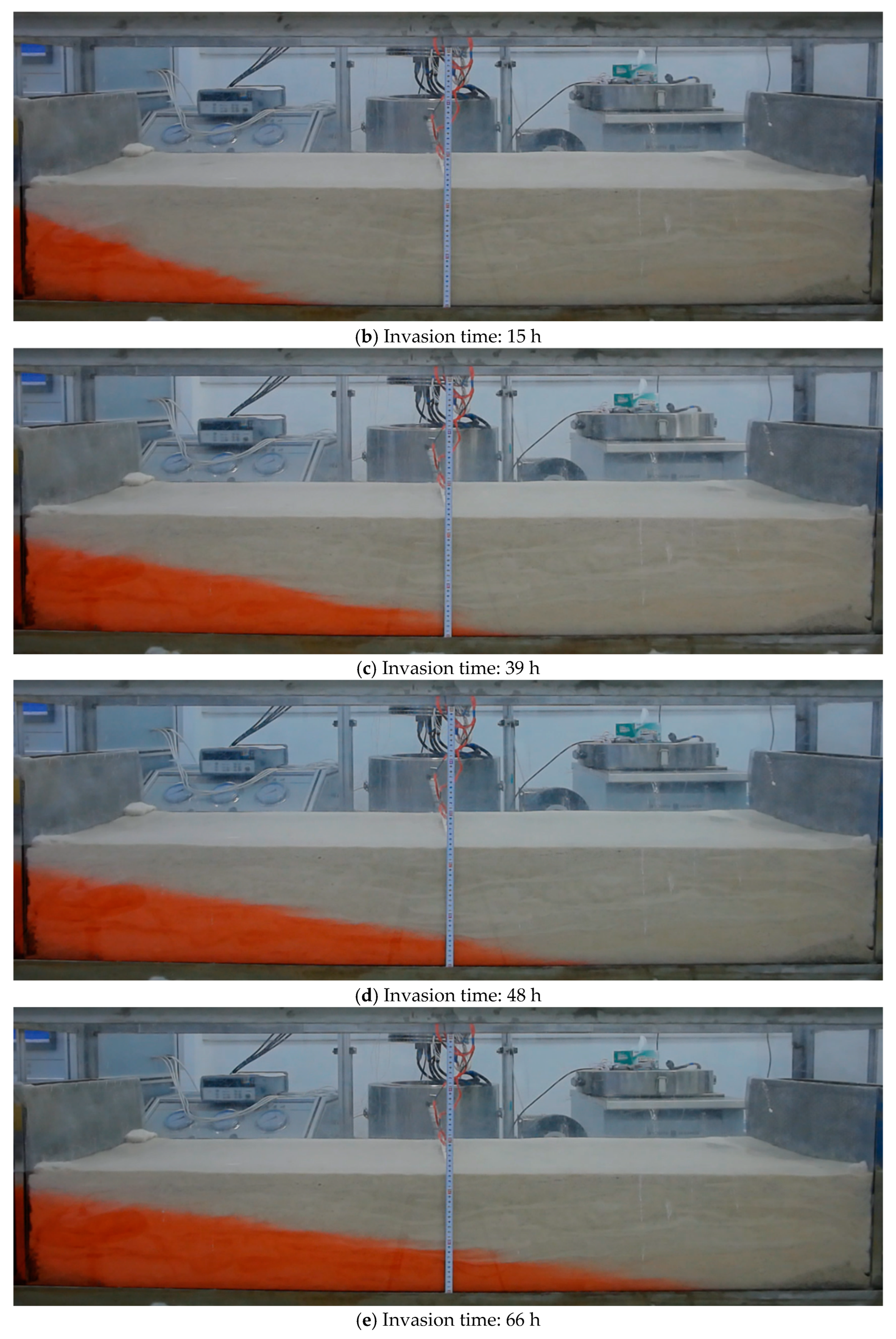
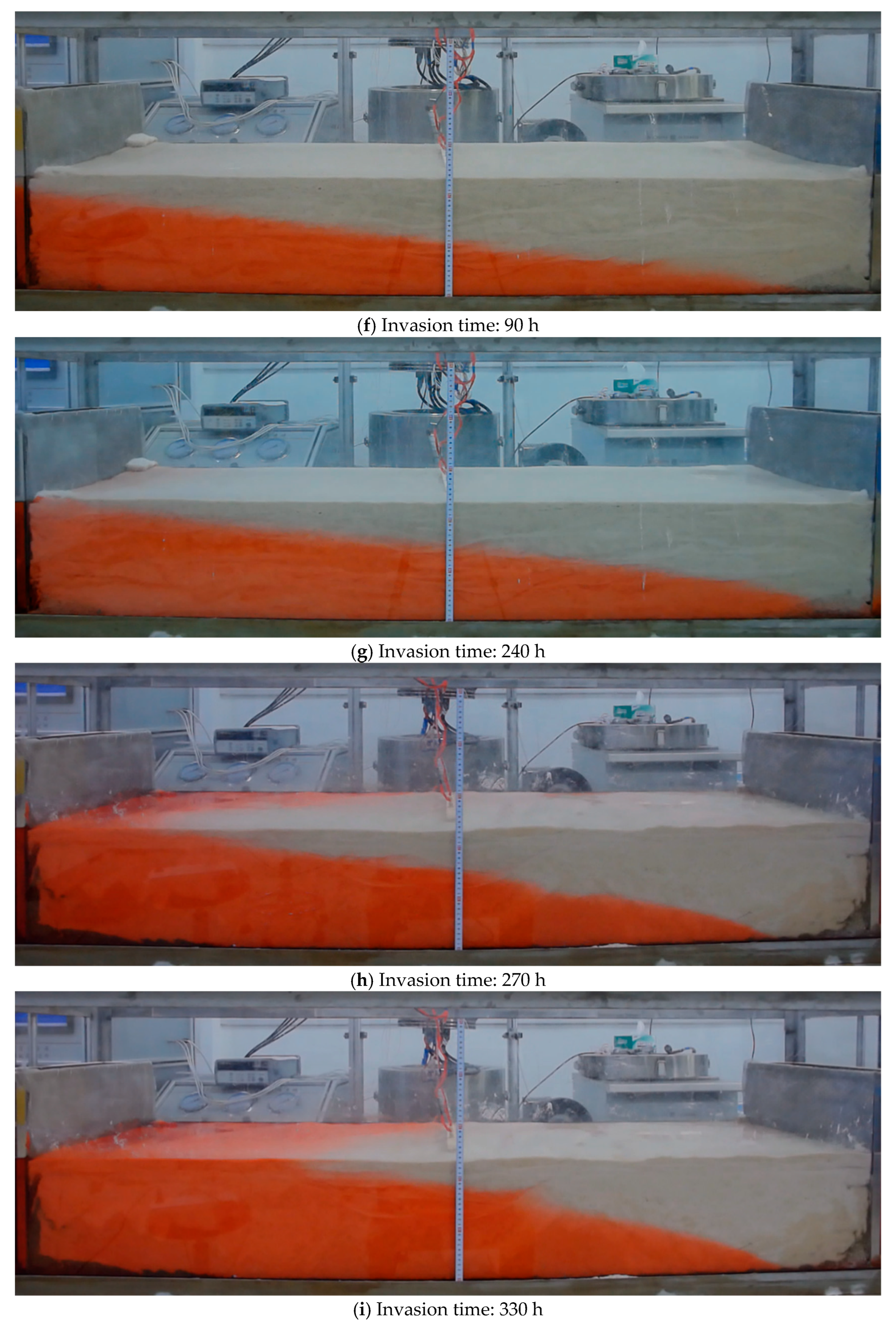
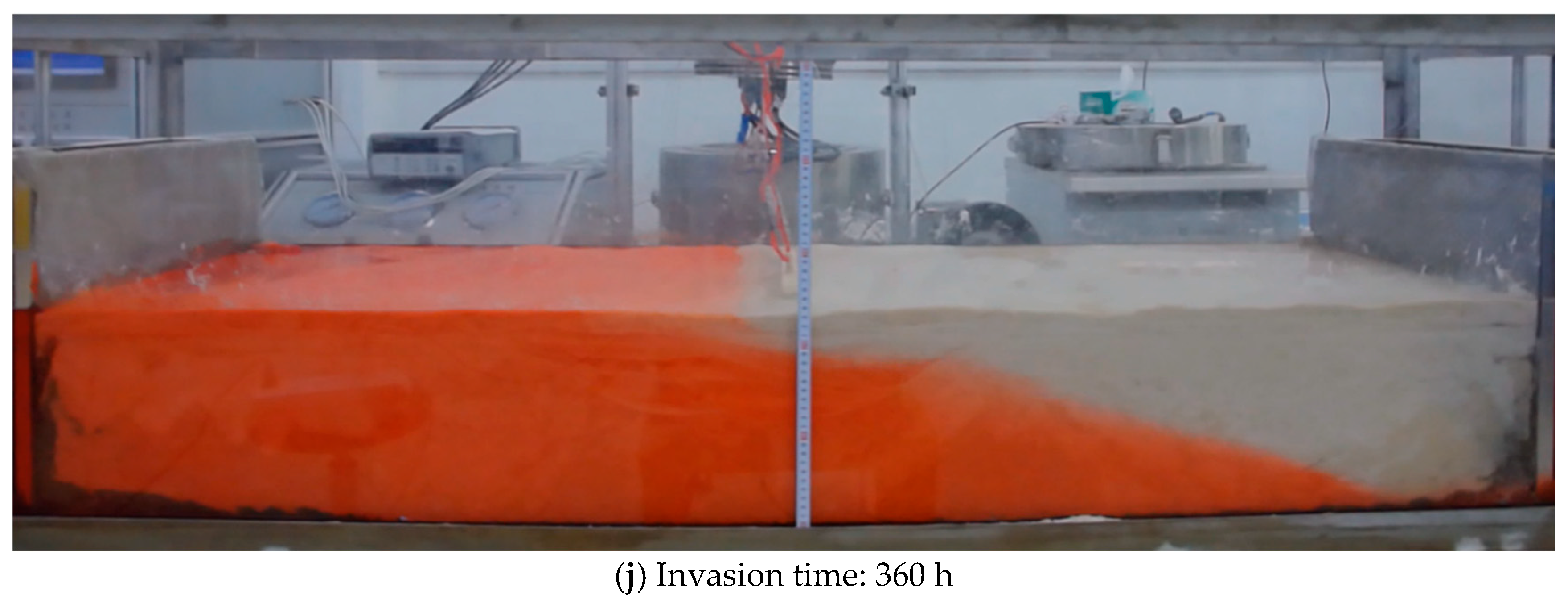
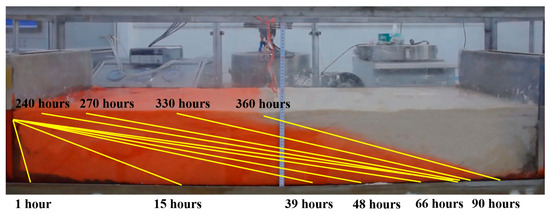
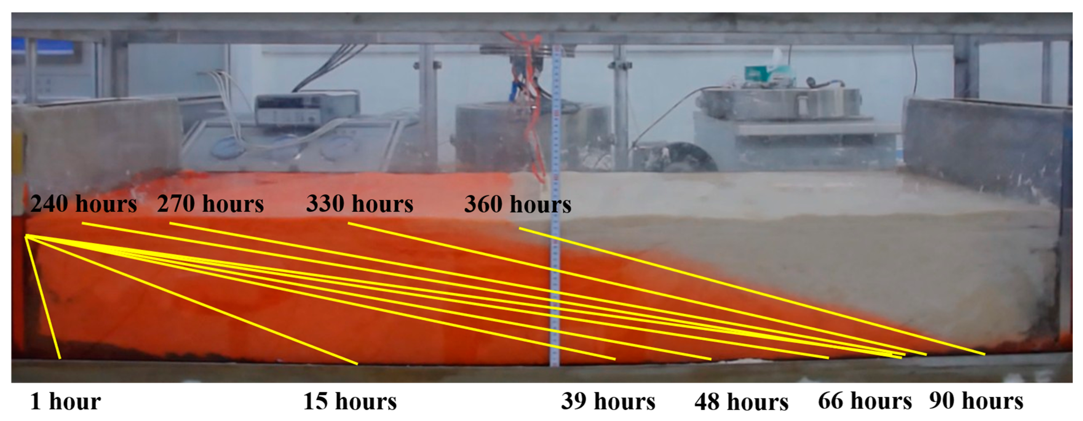
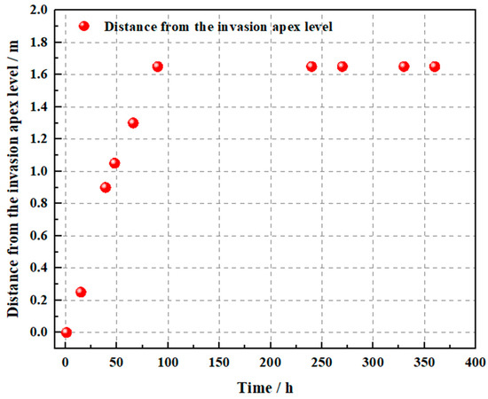
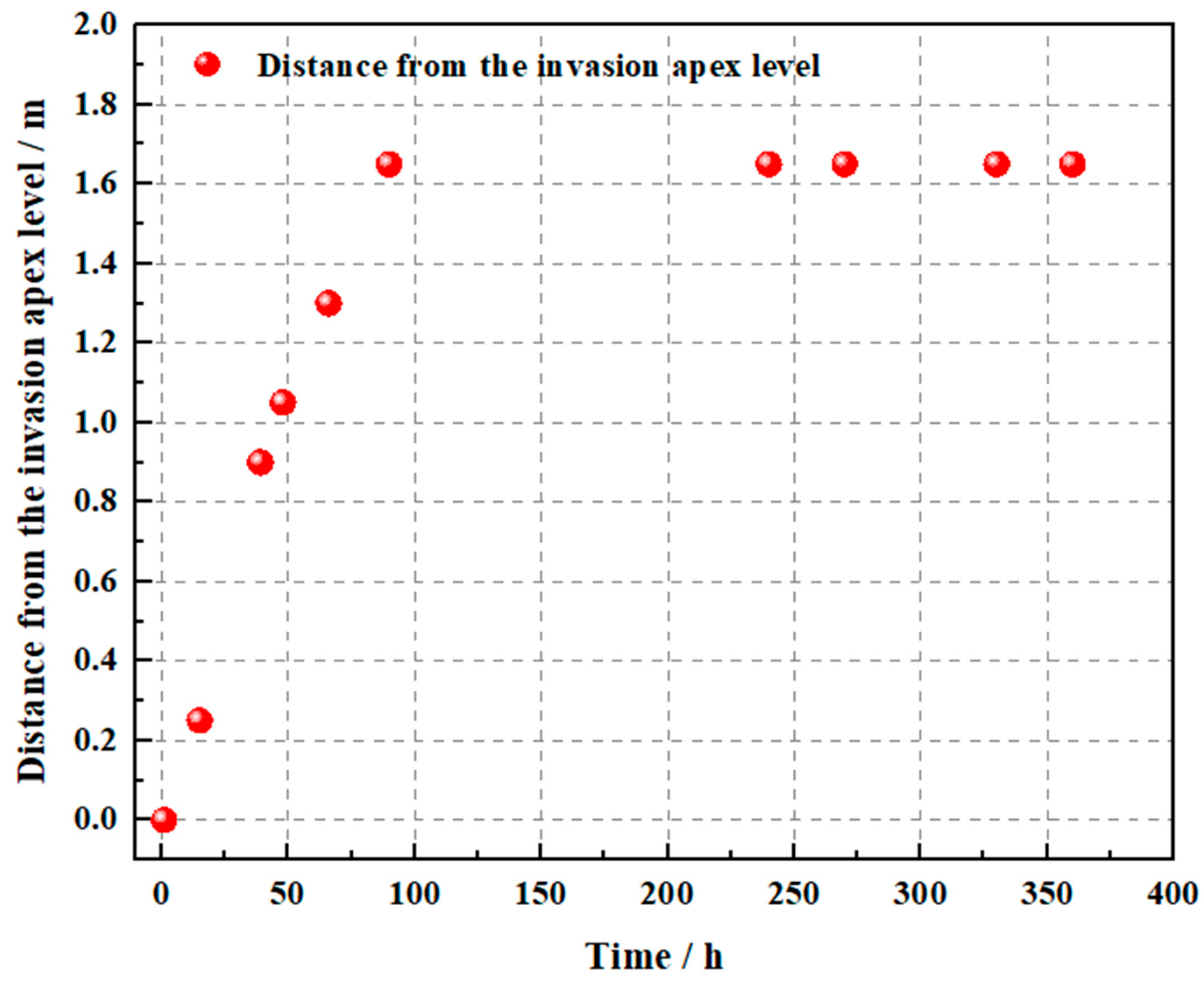
To assess the reliability of the two-dimensional cross-hole resistivity imaging results, the physical distribution of the brine tracer was analyzed based on the Carmine- Red dye visualization (Figure 11, Figure 12 and Figure 13). The seawater intrusion field photographs show that 15 h after intrusion began, the wedge exhibited a triangular shape. The freshwater-seawater boundary appeared as an inclined straight line, forming an angle of approximately 30° with the bottom. Intrusion depth reached 0.04 m near the upper section, 0.25 m at a burial depth of 0.125 m, and approximately 0.45 m at the aquifer base. After 39 h, the wedge morphology changed significantly. Using the 0.125 m burial depth as a reference, the lower portions showed much greater intrusion distances than the upper portions, and the boundary took on an arc-shaped form. At the aquifer base, intrusion reached 0.9 m. At 48 h, the wedge displayed a tongue-shaped pattern, with the bottom intrusion distance reaching 1.05 m. The upper portion showed little change, with intrusion of only 0.05 m at the surface and 0.5 m at the reference line. This demonstrates that, due to hydraulic forces, the lower section exhibited much faster intrusion than the upper section. After 66 h, continuous brine replenishment caused a marked increase in the wedge area. Bottom penetration reached 1.3 m, and intrusion at a burial depth of 0.125 m reached 0.6 m. While intrusion near the surface increased, the changes were smaller. The overall shape of the seawater wedge formed a long, wedge-like structure. After 90 h of seawater intrusion, the seawater wedge continued expanding, with intrusion approaching the surface. The bottom intrusion distance reached 1.65 m, and the intrusion at the 0.125 m depth reached 0.7 m. At 240 h, the wedge area showed little change compared to the previous stage, and intrusion distances stabilized. By 270 h, surface intrusion began. By 360 h, the intrusion front was fully stabilized, showing no further significant movement. This indicates that under constant hydrodynamic conditions, the intrusion process reached a new hydrodynamic equilibrium.

Figure 11. Photographs of the seawater intrusion test setup.

Figure 12. Invasion area change map.

Figure 13. Distance-time variation graph of the horizontal distance from the invasion apex point.

3.2. Resistivity Imaging Characteristics at Different Time Instants

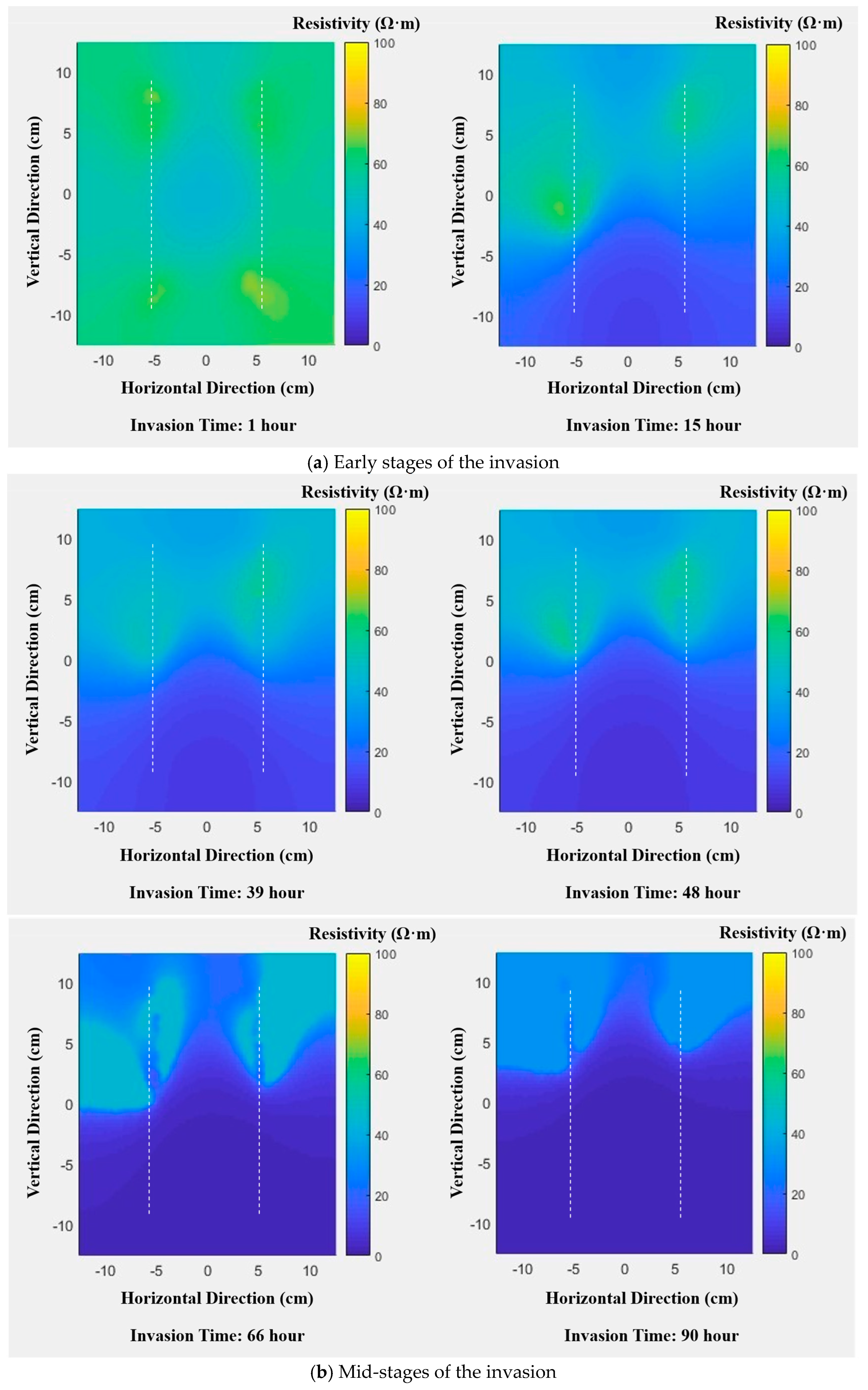
To analyze seawater intrusion from a resistivity perspective, inversion of ERT data was performed from 15 representative monitoring points. Figure 13 presents the resistivity images derived from the inversion of cross-hole electrical resistivity monitoring data collected during 15 surveys. In this experiment, the direction of seawater intrusion is perpendicular to the two electrode components.

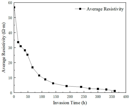
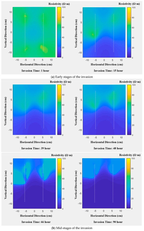
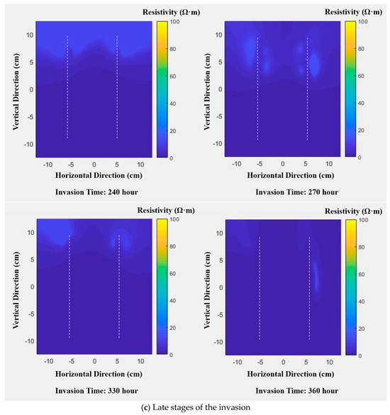
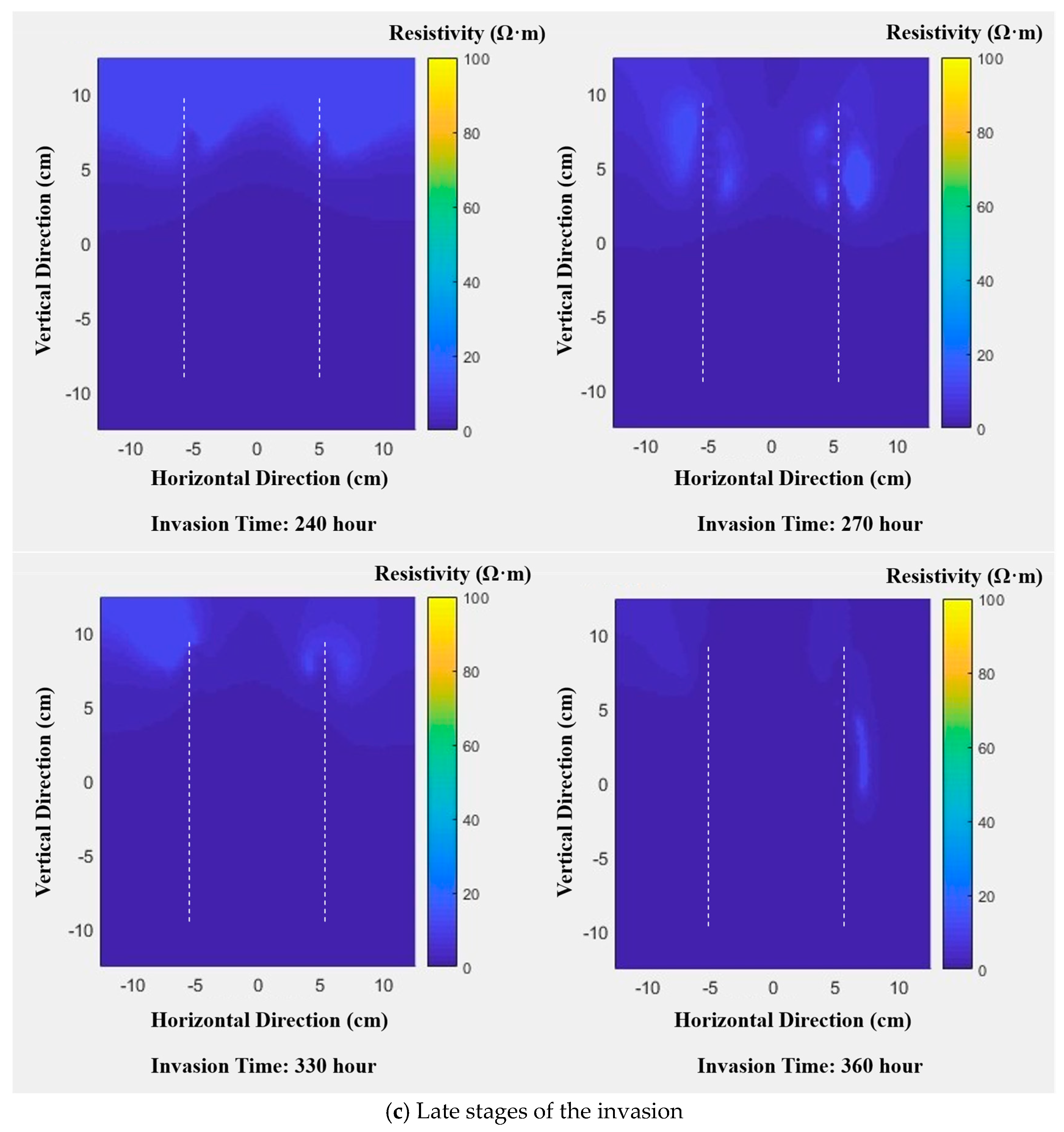
Cross-hole ERT monitoring revealed a strong temporal pattern in resistivity values during seawater intrusion. The average resistivity of the study area declined continuously from 57 Ω·m at the beginning to 1.1 Ω·m at the stabilized stage. Spatial distribution patterns revealed that high-resistivity zones (yellow, orange, and green) corresponding to freshwater gradually contracted, while low-resistivity zones (blue and purple) representing seawater expanded. Seawater progressively invaded from the lower peripheral regions toward the upper and central portions of the aquifer. The resistivity images vividly captured the sequential displacement of freshwater by seawater, illustrating the dynamic evolution of the intrusion process (Figure 14 and Figure 15). Based on these changes, the seawater intrusion process can be broadly divided into three stages: the initial intrusion stage (1–15 h), the intermediate intrusion stage (39–90 h), and the late intrusion stage (240–360 h).

Figure 14. Variation in average resistivity over time.

Figure 15. Resistivity tomography images: (a) early intrusion stage; (b) mid-intrusion stage; (c) late intrusion stage.

The inversion results showed that low-resistivity zones at the base of the aquifer steadily expanded over time. Values in these zones consistently measured below 20 Ω·m, while other regions remained above 30 Ω·m. Based on established relationships between resistivity and salinity, areas with resistivity below 20 Ω·m correspond to zones saturated with saline water. During the early intrusion phase, resistivity began declining but remained above 20 Ω·m on average. In the mid-intrusion stage, low-resistivity areas expanded upward, indicating ongoing freshwater displacement. By the late stage, low-resistivity regions stabilized, reflecting cessation of active brine advancement. These results demonstrate that cross-hole ERT can reliably monitor seawater intrusion and track the migration process.

During the experiment, the sand layer exhibited strong hydraulic connectivity with the saline water. The density difference between saline and freshwater enabled continuous intrusion along the highly permeable sand layer. Simultaneously, as seawater advanced, mixing with freshwater created concentration gradients that further facilitated intrusion via dispersion and diffusion. Continuous replenishment of saline water sustained the expansion of low-resistivity zones, clearly captured by ERT, that advance steadily toward the freshwater side. This characteristic upward progression of low-resistivity zones over time visually reflects the ongoing displacement of original freshwater by saline water within the aquifer.

4. Discussion

4.1. Migration Patterns at the Brackish-Saltwater Interface

The dynamic evolution of the brackish-freshwater interface reflects the coupled mechanism of density-driven transport and diffusion under zero head difference conditions. Experimental results indicate that during the initial phase of seawater intrusion (1–15 h), the interface exhibits a triangular distribution with a bottom angle of approximately 30° relative to the horizontal plane. At this early stage, the density difference between brackish water and seawater serves as the primary driving force. Under gravitational influence, seawater rapidly infiltrates along the aquifer base, producing a bottom intrusion distance of 0.45 m—significantly greater than the upper intrusion distance of 0.04 m. Intrusion was confined to localized areas at greater depths. As intrusion continued (39–48 h), the interface differentiated into an “upper triangular-lower arc-shaped” configuration. The bottom intrusion distance reached 0.9–1.05 m, while the upper zone advanced only about 0.05 m. This strong vertical asymmetry results from persistent gravitational segregation in porous media: denser seawater preferentially occupies lower pore spaces, giving it a migration advantage along the gravitational direction. During the late intrusion phase (240–360 h), the interface gradually expanded upward and stabilized. Intrusion began to appear at the surface, forming an elongated wedge-shaped profile. At this stage, diffusion driven by salinity gradients—rather than density—became the dominant mechanism, thickening the transition zone until a new hydrodynamic equilibrium formed. These observed patterns help address limitations of the traditional Ghyben-Herberg hydrostatic theory, which assumes homogeneity and ignores diffusion effects. The dynamic differentiation of interface morphology documented here provides empirical evidence for understanding seawater intrusion in coastal aquifers under conditions driven by factors other than water level differences.

4.2. Analysis of Two-Dimensional Cross-Hole Electrical Resistivity Characteristics

Dynamic changes at the freshwater-saltwater interface require quantitative characterization using high-precision geophysical monitoring techniques. Two-dimensional cross-hole ERT exhibits high sensitivity to salinity variations and improved resolution, and its imaging results (Figure 15) provide direct visual evidence for interface evolution. During the experiment, low-resistivity zones (<20 Ω·m) consistently corresponded to the extent of saline intrusion: At 1 h (left of Figure 15a), the entire region in the image showed high resistivity characteristics of 80–100 Ω·m, with an average resistivity of 56.83 Ω·m, indicating complete freshwater saturation of the aquifer. As the intrusion progressed, Figure 15a (right, 15 h) to Figure 15b (39–90 h) clearly show that the low-resistivity zone gradually expanded upward from the aquifer base, and the high-resistivity zone continued to shrink. At the stabilized stage of 360 h (right of Figure 15c), the entire region in the image showed uniformly low resistivity (1–5 Ω·m), the average resistivity decreased to 1.14 Ω·m, and the high-resistivity zone (>30 Ω·m) completely disappeared, indicating complete displacement of freshwater. The physical mechanism behind this transition is well understood: the high concentrations of Cl⁻ and Na⁺ in seawater significantly increase pore fluid conductivity, thereby reducing formation resistivity, and resistivity attenuation is positively correlated with saline water saturation.

It should be noted that the insufficient size of the experimental water tank (serving as the reaction kettle in the experiment) may have introduced certain distortions to the monitoring results. Due to the limited internal space of the water tank, the boundary effect of the tank wall exerted an unavoidable influence on the flow field and electric field distribution within the porous medium. Specifically, the seepage path of saline water was restricted by the tank wall, and the electric field generated by the electrode array was distorted near the wall, which may have led to slight deviations in the inversion results of resistivity images, especially in the areas close to the tank wall. Regrettably, this kind of distortion caused by the tank wall belongs to the systematic error of the experimental device itself, and effective correction cannot be achieved through post-measurement data processing. Therefore, in subsequent similar experiments, a water tank (reaction kettle) with a larger volume should be selected. A larger experimental space can minimize the boundary effect of the tank wall, make the seawater intrusion process more consistent with the natural hydrodynamic conditions of actual coastal aquifers, and ensure that the electric field distribution during the ERT monitoring process is more uniform and stable, thereby improving the accuracy and reliability of the monitoring results.

Compared with traditional surface ERT, whose current density exhibits a power-law attenuation pattern, the dual-well vertical electrode array used in this study (24 electrodes per well, dipole-dipole acquisition mode) effectively overcomes this limitation. Direct contact between electrodes and deep strata enables Figure 15 to capture the migration process of the basal saline water tongue with high resolution—at 48 h (second from left in Figure 15b), the horizontal advancement distance of the saline water tongue in the 25 cm thick sand layer reached 1.05 m, with a clearly distinguishable interface morphology. More importantly, the resistivity images at various stages in Figure 15 are highly consistent with the Carmine- Red tracer observations: the trajectory of the tracer showing “bottom-priority intrusion—middle arc-shaped expansion—full-region coverage” is completely consistent with the evolution path of the low-resistivity zone in Figure 15, further verifying the accuracy and reliability of cross-hole ERT for quantifying seawater intrusion processes.

4.3. Analysis of Groundwater Seepage and Migration Characteristics

Quantitative analysis of groundwater seepage and migration is key to revealing the mechanism of seawater intrusion under zero-head-difference conditions. The detailed imaging features in Figure 15 provide intuitive support for migration characteristics: at 48 h (second from left in Figure 15b), the low-resistivity zone showed an obvious tongue-shaped morphology with a “wide bottom and narrow top”, corresponding to a bottom intrusion distance of 1.05 m and an upper intrusion distance of only 0.05 m, presenting a “bottom-priority intrusion” pattern. This disparity arises from the combined effects of density-driven flow and gravitational differentiation: no external hydraulic gradient was applied in the experiment, and the density difference between saline and freshwater (0.025 g/cm³) generated a vertical permeation pressure gradient. According to Darcy’s Law, seawater preferentially advances along the lower pores, with density difference being the main control factor of flux.

In the intermediate intrusion stage (39–90 h), Figure 15b clearly shows that the low-resistivity zone gradually evolved from an arc shape at 39 h (leftmost) to a long wedge shape at 66 h (rightmost) and near full-region coverage at 90 h (second from right), indicating continuous replenishment of saline water rapidly filling the lower pores. The migration rate decreased from 0.0225 m/h at 15 h (corresponding to the length of the low-resistivity zone of 0.45 m in Figure 15a, right) to 0.0194 m/h at 90 h (corresponding to the length of the low-resistivity zone of 1.65 m in Figure 15b, second from right). During this stage, the influence of dispersion became increasingly significant: molecular diffusion and mechanical dispersion driven by concentration gradients increased the thickness of the transition zone from 0.1 m at 15 h (width of the high-resistivity-low-resistivity transition zone in Figure 15a, right) to 0.3 m at 90 h (width of the transition zone in Figure 15b, second from right), further slowing the intrusion rate. In the late stage (after 240 h), Figure 15c shows that the morphology of the low-resistivity zone was basically stable: there was minimal difference between the imaging results at 240 h (leftmost) and 360 h (second from right), with the bottom intrusion distance slightly increasing from 1.65 m to 1.7 m, corresponding to a rate of only 1.16 × 10⁻⁵ cm/s. This stable state indicates that freshwater and saline water in the aquifer reached saturation equilibrium, with seepage and diffusion dynamically offsetting each other. This finding has practical implications for groundwater management in coastal regions: the “bottom-priority intrusion” feature revealed in Figure 15 indicates that the lower aquifer is more sensitive to seawater intrusion when groundwater levels are close to sea level. Deep groundwater extraction may exacerbate upward saline migration and should therefore be carefully managed.

5. Conclusions

This paper addresses the limitations of traditional high-density resistivity imaging methods and the multi-solution nature of geophysical exploration data. It demonstrates the feasibility of monitoring seawater intrusion by integrating two-dimensional cross-hole electrical resistivity tomography, thereby enabling synchronous monitoring of the entire seawater intrusion process. This study was able to conduct synchronous monitoring of the entire seawater intrusion process, analyze the morphology and migration patterns of the freshwater-saltwater interface from a resistivity perspective, and conduct reliability analysis of the results. This approach accurately captures the morphology and migration patterns of the freshwater-saltwater interface during seawater intrusion under zero-head conditions. The methods used here are applicable not only to laboratory sand-flume experiments but also to field-scale monitoring and regional seawater intrusion detection. This dual applicability is a key reason for selecting high-density resistivity imaging for multi-dimensional seawater intrusion monitoring. Based on the results of this study, the following conclusions are drawn:

• Two-dimensional cross-hole ERT technology effectively overcomes the low-depth-resolution bottleneck of traditional surface ERT, providing a high-precision quantitative method for dynamic monitoring of seawater intrusion. The adopted dual-well vertical electrode array (24 electrodes per well) and dipole-dipole acquisition mode achieve direct coupling with deep strata through in-well electrodes, successfully avoiding exponential current decay with depth. This advantage is reflected in Figure 15: millimeter-scale movement of the freshwater-saltwater interface in the 25 cm sand layer is clearly characterized, and the boundary position and morphological changes in the low-resistivity zone at each time point can be accurately captured. Monitoring results show that the average resistivity continuously decreased from 56.83 Ω·m (freshwater state) to 1.14 Ω·m (stable stage), and the low-resistivity zone (<20 Ω·m) spatially corresponds to the extent of saline intrusion; the technology is sensitive to salinity gradient changes on the order of 1 Ω·m, and the imaging results in Figure 15 are highly consistent with Carmine- Red tracer observations. This method overcomes the spatiotemporal constraints of traditional logging techniques and provides a reliable basis for quantitative monitoring of seawater intrusion.
• Based on this monitoring technology, the density-dependent and diffusive mechanisms governing seawater intrusion in sandy aquifers under zero-head conditions are clarified, complementing the limitations of traditional hydrostatic theory. Combined with the imaging characteristics of Figure 15, the intrusion process exhibits three distinct phases. Initial phase (0–15 h): The density difference between saline and freshwater (0.025 g/cm³) dominates seepage, causing saline water to rapidly penetrate along the aquifer base. Figure 15a shows that the interface forms a triangular shape with a 30° inclination, achieving a bottom migration rate of 6.25 × 10⁻⁴ cm/s. The intrusion distance at the aquifer base (0.45 m) is approximately 11 times that at the top (0.04 m). Mid-stage (39–90 h): An “upper triangular-lower arc-shaped” interface morphology emerges (Figure 15b). Due to pore-filling and increased concentration gradients, the migration rate decreases to 0.0194 m/h, with dispersion becoming a secondary driving factor. The bottom intrusion distance reaches 0.9–1.65 m, while the thickness of the transition zone increases from 0.1 m to 0.3 m. Gravity segregation enables sustained rapid advancement in the lower zone, while the upper zone expands only slowly due to dispersion constraints. Late stage (240–360 h): The migration rate decays to 1.16 × 10⁻⁵ cm/s. Dominated by dispersion, the interface expands upward until stabilization, forming a new hydrodynamic equilibrium with a long wedge-shaped distribution (Figure 15c). These findings correct the omission of heterogeneity and dispersion effects in the Ghyben-Herberg formula, providing empirical evidence for freshwater-saltwater migration in coastal aquifers without hydrostatic head driving forces.
• The technical framework of “technological innovation-experimental simulation-method validation” developed in this study has strong universality and practical value for groundwater safety management in coastal regions. Cross-hole ERT is applicable not only to meter-scale indoor experiments but also to regional-scale field monitoring. Its optimized forward modeling (finite element method) and inversion (Gauss-Newton) algorithms successfully address the multi-solution issues common in traditional geophysical approaches. The imaging results in Figure 15 clearly reveal the high vulnerability of the lower aquifer: saline water will preferentially intrude from below when groundwater levels are close to sea level. Thus, deep groundwater extraction should be carefully managed to prevent upward saline migration. Furthermore, the quantified relationship between resistivity and salinity saturation—where the average resistivity decreases from 56.83 Ω·m to 1.14 Ω·m as freshwater is fully displaced—provides a basis for classifying the severity of seawater intrusion and setting early-warning thresholds.

This experiment employed an experimental approach distinct from previous studies to characterize seawater intrusion in meter-scale indoor flumes. However, not all influencing factors were fully considered. Seawater intrusion includes substantial changes in the aquifer’s physical parameters and hydrochemical composition, all of which affect resistivity. Future studies should investigate these components in more detail to further enhance the reliability of the findings. This experiment, based on actual outdoor seawater intrusion studies characterized by significant duration and complexity, was conducted in a controlled indoor environment using standard test sand to simulate a confined aquifer, which differs significantly from natural geological strata. In reality, seawater intrusion is influenced by multiple factors, including aquifer heterogeneity, boundary water-level fluctuations, temperature variations, and differing recharge sources. Future research will incorporate these factors, drawing on the latest literature, to achieve more robust and comprehensive research outcomes.

References

- Kazakis, N.; Pavlou, A.; Vargemezis, G. Seawater intrusion mapping using electrical resistivity tomography and hydrochemical data. An application in the coastal area of eastern Thermaikos Gulf, Greece. Sci. Total Environ. 2016, 543, 373–387. [Google Scholar] [CrossRef] [Scilit] [PubMed]
- Han, D.M.; Song, X.F.; Currell, M.J.; Yang, J.L.; Xiao, G.Q. Chemical and isotopic constraints on evolution of groundwater salinization in the coastal plain aquifer of Laizhou Bay, China. J. Hydrol. 2014, 508, 12–27. [Google Scholar] [CrossRef] [Scilit]
- Barlow, P.M.; Reichard, E.G. Saltwater intrusion in coastal regions of North America. Hydrogeol. J. 2010, 18, 247–260. [Google Scholar] [CrossRef] [Scilit]
- Yu, P.; Liu, H.H.; Wang, Z.S.; Fu, J.; Zhang, H.; Wang, J.; Qi, Y. Development of urban underground space in coastal cities in China: A review. Deep Undergr. Sci. Eng. 2023, 2, 148–172. [Google Scholar] [CrossRef] [Scilit]
- Liu, X.; Liu, H.; Dong, J.; Yu, P.; Liu, H.; Cheng, G. Land-Sea Integrated Suitability Evaluation of Underground Space based on Pythagorean Fuzzy Bayesian Network. Undergr. Space 2025, 24, 197–215. [Google Scholar] [CrossRef] [Scilit]
- Rumer, R.R. Intruded Salt-Water Wedge in Porous Media. J. Hydraul. Div. 1963, 89, 193–220. [Google Scholar] [CrossRef] [Scilit]
- Kuan, W.K.; Jin, G.; Xin, P.; Clare, R.; Badin, G.; Li, L. Tidal influence on seawater intrusion in unconfined coastal aquifers. Water Resour. Res. 2012, 48, 136–149. [Google Scholar] [CrossRef] [Scilit]
- Lu, C.; Chen, Y.; Zhang, C.; Luo, J. Steady-state freshwater–seawater mixing zone in stratified coastal aquifers. J. Hydrol. 2013, 505, 24–34. [Google Scholar] [CrossRef] [Scilit]
- Brunet, P.; Clément, R.; Bouvier, C. Monitoring soil water content and deficit using Electrical Resistivity Tomography (ERT)—A case study in the Cevennes area, France. J. Hydrol. 2010, 380, 146–153. [Google Scholar] [CrossRef] [Scilit]
- Binley, A.; Cassiani, G.; Middleton, R.; Winship, P. Vadose zone flow model parameterisation using cross-borehole radar and resistivity imaging. J. Hydrol. 2002, 267, 147–159. [Google Scholar] [CrossRef] [Scilit]
- Sonkamble, S. Electrical Resistivity and Hydrochemical Indicators Distinguishing Chemical Characteristics of Subsurface Pollution at Cuddalore Coast, Tamil Nadu. J. Geol. Soc. India 2014, 83, 535–548. [Google Scholar] [CrossRef] [Scilit]
- Naidu, L.S.; Mahesh, J.; Padalu, G.; Sarma, V.S.; Prasad, P.R.; Rao, S.M. An integrated approach to investigate saline water intrusion and to identify the salinity sources in the Central Godavari delta, Andhra Pradesh, India. Arab. J. Geosci. 2012, 6, 3709–3724. [Google Scholar] [CrossRef] [Scilit]
- Atwia, M.G.; Masoud, A.A. Hydrochemical and geoelectrical investigation of the coastal shallow aquifers in El-Omayed area, Egypt. Environ. Monit. Assess. 2013, 185, 7065. [Google Scholar] [CrossRef] [Scilit]
- Yang, C.H.; Tong, L.T.; Huang, C.F. Combined Application of Dc And TEM to Sea-water Intrusion Mapping. Geophysics 1999, 64, 417. [Google Scholar] [CrossRef] [Scilit]
- Tang, X.Q.; Dong, J.; OHTOSHI, K.; Li, J. Survey on fresh-saline groundwater interface in coastal aquiferswith electrical techniques. Hydrogeol. Eng. Geol. 2007, 34, 38–43. [Google Scholar]
- Hodlur, G.K.; Dhakate, R.; Sirisha, T.; Panaskar, D.B. Resolution of freshwater and saline water aquifers by composite geophysical data analysis methods. Int. Assoc. Sci. Hydrol. Bull. 2010, 55, 414–434. [Google Scholar] [CrossRef] [Scilit]
- Zhao, Z.K.; Jia, Y.G.; Guo, L. Experimental Research on Monitoring of Seawater Intrusion Process Using High-density Resistivity Probe. J. Eng. Geol. 2012, 20, 868–876. [Google Scholar]
- Najib, S.; Fadili, A.; Mehdi, K.; Joelle, R.; Makan, A. Contribution of hydrochemical and geoelectrical approaches to investigate salinization process and seawater intrusion in the coastal aquifers of Chaouia, Morocco. J. Contam. Hydrol. 2017, 198, 24–36. [Google Scholar] [CrossRef] [Scilit]
- Yu, P.Z.; Zhang, Z.Y.; Huang, L.P.; Lou, K.F.; Liang, R.N. 2.5D inversion of borehole and surface multi-electrode DC data using unstructured mesh. Prog. Geophys. 2019, 34, 1687–1693. [Google Scholar]
- Shen, P.; Qiang, J.K.; Li, Y.J.; Ruan, B.Y. Geometry image method of crosshole apparent resistivity. J. Cent. South Univ. (Sci. Technol.) 2010, 41, 1079–1084. [Google Scholar]
- Álvarez-Alonso, R.; Robledo Ardila, P.A.; Deudero, S.; Melo-Aguilar, C.A.; Alomar, C.; Micheo, F.; Durán, J.J.; Pérez, S.; Árcega Cabrera, F.; Martínez Pérez, S. Multivariate assessment of groundwater contamination levels associated with saline intrusion processes in Mediterranean coastal aquifers. J. Contam. Hydrol. 2026, 278, 104877. [Google Scholar] [CrossRef] [Scilit]
- Slater, L.D.; Binley, A.M.; Daily, W.D.; Johnson, R. Cross-hole electrical imaging of a controlled saline tracer injection. J. Appl. Geophys. 2000, 44, 85–102. [Google Scholar] [CrossRef] [Scilit]
- Schmidt-Hattenberger, C.; Bergmann, P.; Bösing, D.; Labitzke, T.; Möller, M.; Schröder, S.; Wagner, F.; Schütt, H. Permanent Downhole Geoelectrical Monitoring at the Ketzin CO2 Pilot Site. In Proceedings of the 75th EAGE Conference & Exhibition incorporating SPE EUROPEC, London, UK, 10–13 June 2013. [Google Scholar]
- Jensen, K.H.; Haarder, E.B.; Binley, A.; Nielsen, L.; Uglebjerg, T.B.; Looms, M.C. Estimation of Recharge from Long-Term Monitoring of Saline Tracer Transport Using Electrical Resistivity Tomography. Vadose Zone J. 2015, 14, vzj2014-08. [Google Scholar]
- Perri, M.T.; Cassiani, G.; Gervasio, I.; Deiana, R.; Binley, A. A saline tracer test monitored via both surface and cross-borehole electrical resistivity tomography: Comparison of time-lapse results. J. Appl. Geophys. 2011, 79, 6–16. [Google Scholar] [CrossRef] [Scilit]
- Kiessling, D.; Schmidt-Hattenberger, C.; Schuett, H. Geoelectrical methods for monitoring geological CO2 storage: First results from cross-hole and surface-downhole measurements from the CO2SINK test site at Ketzin (Germany). Int. J. Greenh. Gas Control 2010, 4, 816–826. [Google Scholar] [CrossRef] [Scilit]
- Schmidt-Hattenberger, C.; Bergmann, P.; Labitzke, T.; Wagner, F. CO2 migration monitoring by means of electrical resistivity tomography (ERT)-Review on five years of operation of a permanent ERT system at the Ketzin pilot site. Energy Procedia 2014, 63, 4366–4373. [Google Scholar] [CrossRef] [Scilit]
- Utada, H.; Koyama, T.; Obayashi, M.; Fukao, Y. A joint interpretation of electromagnetic and seismic tomography models suggests the mantle transition zone below Europe is dry. Earth Planet. Sci. Lett. 2009, 281, 249–257. [Google Scholar] [CrossRef] [Scilit]
- Sufiyanussuari, A.; Tajudin, A.; Azmi, S.; Zahari, H.; Muztaza, M. Groundwater pathway mapping using electrical resistivity tomography (ERT) method. J. Sustain. Undergr. Explor. 2021, 1, 32–37. [Google Scholar] [CrossRef] [Scilit]
- Jiang, F.Y.; Ni, J.; Chen, H.J.; Gao, L.K.; Chen, S.; Wu, X.W. Resistivity tomography based on multichannel electrodes. Appl. Geophys. 2024, 21, 4–18. [Google Scholar] [CrossRef] [Scilit]
- Wang, Z.G.; He, Z.X.; Wei, W.B. Parallel Algorithm Research of Integral Equation Method to 3-D Borehole Surface Electromagnetic Modeling. Comput. Tech. Geophys. Geochem. Explor. 2007, 29, 425–430. [Google Scholar]
- Petrick, W.R.; Sill, W.R.; Wards, S.H. Three-dimensional resistivity inversion using alpha centers. Geophysics 1981, 46, 1148. [Google Scholar] [CrossRef] [Scilit]
- Dey, A. Resistivity modeling for arbitrarily shaped three-dimensional structures. Geophysics 1979, 44, 106–136. [Google Scholar] [CrossRef] [Scilit]
- Jackson, P.D.; Earl, S.J.; Reece, G.J. 3D resistivity inversion using 2D measurements of the electric field. Geophys. Prospect. 2010, 49, 26–39. [Google Scholar] [CrossRef] [Scilit]
- Schmidt-Hattenberger, C.; Bergmann, P.; Labitzke, T.; Wagner, F.; Rippe, D. Permanent crosshole electrical resistivity tomography (ERT) as an established method for the long-term CO2 monitoring at the Ketzin pilot site. Int. J. Greenh. Gas Control 2016, 52, 432–448. [Google Scholar] [CrossRef] [Scilit]
- Wagner, F.M.; Günther, T.; Schmidt-Hattenberger, C.; Maurer, H. Constructive optimization of electrode locations for target-focused resistivity monitoring. Geophysics 2015, 80, 29–40. [Google Scholar] [CrossRef] [Scilit]
- Shima, H.; Sakayama, T. Resistivity tomography: An approach to 2-D resistivity inverse problems. In SEG Technical Program Expanded Abstracts, Proceedings of the 1987 SEG Annual Meeting, New Orleans, LA, USA, 11–15 October 1987; Society of Exploration Geophysicists: Houston, TX, USA, 1987; Volume 1, pp. 59–61. [Google Scholar]
- Loke, M.H.; Barker, R.D. Improvements to the Zohdy method for the inversion of resistivity sounding and pseudosection data. Comput. Geosci. 1995, 21, 321–332. [Google Scholar] [CrossRef] [Scilit]
- Yorkey, T.J.; Webster, J.G.; Tompkins, W.J. Comparing Reconstruction Algorithms for Electrical Impedance Tomography. IEEE Trans. biomed. Eng. 1987, 34, 843–852. [Google Scholar] [CrossRef] [Scilit] [PubMed]
Disclaimer/Publisher’s Note: The statements, opinions and data contained in all publications are solely those of the individual author(s) and contributor(s) and not of MDPI and/or the editor(s). MDPI and/or the editor(s) disclaim responsibility for any injury to people or property resulting from any ideas, methods, instructions or products referred to in the content. |
© 2026 by the authors. Licensee MDPI, Basel, Switzerland. This article is an open access article distributed under the terms and conditions of the Creative Commons Attribution (CC BY) license.