Leader–Follower Motion Control System for a Group of AUVs via Hybrid Measurement Sparse LBL Navigation

Abstract

Autonomous navigation of underwater vehicles in infrastructure-limited environments presents persistent challenges due to the constraints of traditional acoustic positioning systems. Sparse long baseline (sparse LBL) navigation, which relies on a minimal set of acoustic transponders, offers a promising alternative but suffers from geometric ambiguity and reduced robustness without external aiding. This paper introduces an integrated approach to measurement-based navigation and control in the sparse LBL setting with two base transponders, focusing on three key components. First, a novel three-stage navigation algorithm is proposed, which enables unambiguous robust leader–follower formation position estimation using only two acoustic transponders and onboard measurements. Second, a hybrid state estimation framework is developed to fuse asynchronous data from inertial sensors, depth measurements, and acoustic ranging, accommodating measurement uncertainty and timing variability. Third, there is a nonlinear trajectory tracking controller based on state-dependent coefficients (SDCs) technique. The combined approach enables accurate and robust leader–follower structure navigation with minimal acoustic infrastructure and is suitable for deployment in dynamic or remote underwater scenarios. The numerical simulations demonstrate the acceptable motion control accuracy.

1. Introduction

The accurate navigation and control of autonomous underwater vehicles (AUVs) remain critical challenges, especially in environments where the deployment of full-scale acoustic infrastructure is impractical. Traditional long baseline (LBL) systems ensure high positioning accuracy through triangulation from multiple fixed seabed transponders. However, such systems require substantial installation efforts and logistical support, which constrain their applicability in dynamic or cost-sensitive missions.

Sparse LBL configurations, which employ as few as two seabed transponders, have been advanced as a flexible alternative to dense LBL arrays. Commercial solutions include Kongsberg’s HiPAP sparse LBL [1], which fuses LBL ranges with surface-based SSBL fixes and depth to form a weighted solution, and explicitly supports two-transponder operation; Exail’s (iXblue) Canopus/Ramses concept of sparse LBL [2], which tightly couples Ramses range updates with an onboard INS; and Sonardyne’s Fusion 2 toolchain [3], which provides real-time calibration and workflows tailored to sparse LBL deployments. Despite their practicality, these approaches often depend on favorable geometry, external aiding data, and strict timing; moreover, asynchronous updates and mismatched sensor data rates complicate state estimation and feedback design.

To address these limitations, a hybrid navigation and control framework is proposed. The approach integrates a novel three-stage acoustic localization method with a measurement-driven state estimation architecture and a nonlinear trajectory tracking controller. The localization algorithm is designed for configurations with minimal acoustic infrastructure and provides position estimates based solely on one-way travel time (OWTT) from acoustic transponders and onboard measurements. These estimates are incorporated into a hybrid estimator that fuses asynchronous data from inertial sensors, pressure sensors, and acoustic range measurements. For trajectory tracking, the control scheme employs a nonlinear state-dependent coefficients formulation [4], allowing for real-time optimal control synthesis based on the current estimated state.

Long baseline (LBL) acoustic positioning traditionally requires an array of seabed transponders (typically 3–4) to triangulate an underwater vehicle’s position. Recent efforts have focused on sparse LBL systems that achieve comparable accuracy with far fewer transponders [5]. For example, modern sparse LBL solutions can use a single fixed transponder coupled with a high-quality inertial navigation system (INS) on the AUV, fusing precise one-way range measurements with the vehicle’s short-term inertial dead-reckoning to continuously bound position error. This approach, employed in systems like iXblue/Exail’s Canopus/Ramses, yields performances rivaling conventional LBL while significantly reducing the deployment effort [6]. Moreover, advanced “virtual LBL” techniques allow an AUV to treat its own past poses as surrogate transponders: for instance, González-García et al. [7] used a single seafloor sound source and the AUV’s recent trajectory to form a virtual four-transponder LBL network, achieving positioning accuracy on the order of 2 m in simulation. Similarly, range-only localization methods have been demonstrated using minimal transponder infrastructure—Masmitja et al. report that an AUV can do homing with <4 m error by using a single moving surface vehicle (wave-glider) as a mobile LBL transponder and carefully optimizing its survey pattern (e.g., ≥12 waypoints over a ~400 m radius trajectory). These sparse LBL approaches illustrate the feasibility of minimal acoustic infrastructure, but they also highlight some challenges. Because fewer simultaneous ranges are available, the vehicle must often maneuver to gain observability; maintaining continuous motion is necessary to refine the solution and avoid unbounded drift in single-transponder configurations. In addition, acoustic propagation effects can degrade accuracy; however, none of the above studies fully resolves issues like multipath interference or spatially variable sound speed, which can induce bias in range measurements [8].

Beyond fixed-transponder LBL, a broad class of measurement-based localization methods rely on in situ sensor data such as inter-vehicle acoustic communication signals, one-way travel time ranges, depth readings, and inertial outputs to estimate an AUV’s position in real time. A common scenario is an AUV navigating with a single acoustic transponder (for example, a surface ship or fixed transponder) providing range updates via acoustic transponder signals. Several studies since 2015 have advanced range-only localization algorithms for this scenario. Vallicrosa and Ridao [9] developed a Sum-of-Gaussians filter for single-transponder range measurements and demonstrated robust homing of an AUV to an acoustic target with final position errors under 4 m. Yuan et al. [10] proposed a fast single-transponder localization algorithm that improves computational efficiency for real-time use, while others have explored moving horizon estimation and particle filters to handle the nonlinear observability problem of range-only navigation. In practice, auxiliary sensors like depth gauges (pressure sensors) are invariably used alongside acoustics—knowing a vehicle’s depth allows one to constrain the 3D solution and reduce ambiguity when only one or two range measurements are available. Inertial sensors (IMU/INS) further provide high-frequency dead-reckoned pose estimates that can be aided by intermittent acoustic fixes [10]. Indeed, most modern systems fuse acoustics with inertial data: for example, Garin et al. [5] describe a low-cost AUV positioning system where a single acoustic transponder range (ToF) is combined with the AUV’s depth and Doppler-measured velocity to correct INS drift. Such systems can leverage the Doppler shift in the acoustic communication signals themselves to estimate relative velocity, simultaneously achieving communication and navigation goals. Recent field trials have validated simultaneous acoustic communication and localization (Simultaneous Localization and Communication, SLaC): Diamant et al. [11] introduced the idea of embedding Doppler-based velocity measurements in acoustic network nodes, and more recently, Aubry et al. [12] demonstrated that an AUV can decode a data packet from a single transponder and extract both range (from propagation time) and its relative speed (from Doppler shift) to update its position filter. Garin et al. [5] extended this concept with sea experiments, showing that a single-transponder acoustic link can reliably provide periodic range and velocity observations to an EKF-based AUV navigation system. Performance comparisons indicate that purely dead-reckoned navigation (INS alone) accumulates unbounded error, while adding even infrequent range measurements bounds the drift. However, range-only schemes come with trade-offs: with a single transponder, the position solution is unobservable without vehicle motion, and strong ocean currents can induce significant localization errors if not modeled. Researchers have found that integrating water-current velocity sensors or DVL can compensate for this; for instance, purely range-based positioning yields large errors unless aided by a Doppler velocity log, which can reduce the sensitivity to unmodeled currents. In summary, measurement-based localization approaches using acoustic transponders and minimal infrastructure are attractive for their low cost and simplicity, and recent advances (fast algorithms, comm-based ranging) have improved their viability. Yet, the accuracy and robustness of these methods still often lag behind multi-transponder LBL or USBL systems, especially in challenging environments. This gap motivates the present work to fuse such measurements in a more sophisticated state estimation framework and to leverage control strategies that can tolerate occasional position uncertainty.

Given the complementary strengths of acoustic and inertial sensors, hybrid state estimation techniques have been extensively investigated to fuse asynchronous, multi-rate data streams for underwater navigation. AUV INSs provide high-rate pose updates (often 10–100 Hz) but suffer unbounded drift, whereas acoustic range fixes (LBL, USBL, or single-transponder ToF) arrive at low rates (typically one measurement every few seconds) and often with latency due to acoustic travel times. This temporal disparity poses a non-trivial filtering problem: the vehicle’s state may evolve significantly between acoustic updates, and each range measurement may correspond to a past state (in two-way ranging, the measurement relates to the vehicle’s position at signal transmission and reception instants) [13]. To address these challenges, researchers have developed asynchronous filtering algorithms and smoothing techniques. One approach is the use of delayed-state Kalman filters, which explicitly augment the state to include past vehicle positions at the time of acoustic transmission, as in the work of Ribas et al. [14] for USBL-aided INS. Another approach is adaptive filtering with multi-rate updates: Davari and Gholami [15] presented an asynchronous adaptive Kalman filter for an integrated INS/DVL/depth/GPS system, allowing each sensor to update at its own rate with time-varying noise statistics. In field experiments, their adaptive filter reduced the RMS navigation error by about 61% compared to a standard (synchronously tuned) Kalman filter. Similarly, Yang et al. [16] implemented a parallel federated filtering scheme (using dual unscented Kalman filters) to fuse the acoustic range and vision data with INS, demonstrating efficient computation and improved accuracy in post-processing. Beyond Kalman approaches, factor graph and smoothing methods (e.g., pose SLAM algorithms using acoustic loop closures) have been applied to batch-process asynchronous measurements for improved consistency [17]. The literature also shows interest in state estimation robustification against sporadic or out-of-sequence data: for instance, multi-model filters and particle filters have been used to handle abrupt changes or delayed observations in AUV navigation [7]. Despite these advances, challenges remain. Many integrated systems, including earlier LBL/INS combinations, assumed perfect acoustic time-sync and did not fully address issues like multipath biases or environmental sound-speed variation, often treating them as random noise. As noted in one study, even a “near-real-time” tightly coupled LBL/INS filter with an asynchronous ping schedule suffered from uncorrected bias when faced with multipath correlations and refraction errors [13]. This highlights a gap in the existing state estimation frameworks of handling environmental uncertainties and out-of-sequence data in a principled way. In our work, we build on the hybrid fusion paradigm by adopting an estimation scheme that can accommodate asynchronous acoustic inputs and account for their unique error characteristics. This is expected to enhance the navigation accuracy without the need for dense transponder infrastructure.

Leader–follower formations are a standard coordination architecture in multi-AUV systems because they align naturally with directed, broadcast-style communication under severe underwater constraints (low rate, high latency, Doppler). In such structures, a designated leader supplies a reference trajectory and coordination cues, while followers regulate relative motion to maintain the prescribed geometry. Reviews of AUV formation control consistently enumerate leader–follower alongside consensus, virtual-structure, and behavior-based schemes, and emphasize that the communication model strongly conditions attainable performance and robustness. Under OWTT constraints, a synchronous cycle in which all vehicles acquire common ranging observables and then receive a single broadcast of control information is particularly effective; it yields deterministic latency and group size-independent update times [18].

Accurate state estimation must be complemented by a robust control strategy to ensure an AUV follows the desired trajectories despite environmental disturbances and model uncertainties. AUV trajectory tracking is inherently a nonlinear control problem (due to coupled 6-DoF vehicle dynamics and actuator constraints), and a variety of control techniques have been proposed post-2015, ranging from adaptive and robust methods to optimal control formulations. Classical approaches like backstepping, sliding mode control (SMC), and H∞ robust control have seen continual refinements—for example, recent adaptive terminal sliding mode controllers can achieve finite time convergence and reject disturbances in 6-DOF AUVs [19]. Alongside these, optimal control methods have gained traction for their ability to systematically handle nonlinearities and constraints. One prominent method is the state-dependent coefficients (SDCs) technique, which generalizes the linear quadratic regulator (LQR) to nonlinear systems by solving a state-dependent riccati equation (SDRE) on-the-fly, using the current state to parameterize the system matrices. SDRE-based controllers have been successfully applied to AUVs. Geranmehr and Nekoo (2015) demonstrated a full 6-DoF SDRE controller on a non-affine AUV model without the common practice of decoupling dynamics; their suboptimal SDRE feedback law kept the vehicle’s position error to merely ~0.04 m over an 8.77 m horizontal excursion (i.e., <0.5% error) in simulation [20]. This highlighted the potential of SDRE for high-precision tracking.

In terminal problems on a finite interval, a Riccati differential equation (SDDRE) arises [21]. The classical solution requires its backward integration, which in the nonlinear case (unlike the linear case) is impossible without knowledge of the future state trajectory and control. Existing approaches either use single-step direct procedures (based on the Lyapunov equation, transition matrix [22,23]), which give approximations, or two-step procedures with backward integration, where, in the reverse direction, either a stabilizing or a terminal control law is additionally used [21,24].

A similar problem arises in finite interval tracking problems for nonlinear systems in SDC formulation [25,26]. Optimal control here contains a feedback term (dependent on the state) and a feedforward term (dependent on the reference signal). To calculate the latter in classical linear quadratic tracking (LQT), reverse integration with boundary conditions on the right end is also required, which in the nonlinear case faces the same problem of the future state uncertainty.

To overcome the indicated problem of the unknown state vector during backward integration, this paper uses nonlinear differential equations of optimal control in forward time (NDOCE FT) [27]. The NDOCE FT approach is based on deriving a solution through the corresponding differential equations for the Riccati-type matrix and the auxiliary vector, the initial conditions for which are uniquely specified at the left end of the time interval due to the use of a special Riccati transform, which is different from the typical one. This allows calculating the control through the integration of the corresponding differential equations in forward time, which removes the problem of the unknown state vector.

In summary, contemporary AUV control research offers a suite of nonlinear control approaches. Optimal control formulations (SDC, MPC, etc.) stand out for enabling systematic performance tuning and multi-objective optimization (e.g., tracking accuracy and energy efficiency [19]), but they introduce complexity and potential fragility (local stability, heavy computing demand). This leaves room for hybrid control schemes that combine the real-time robustness of classical controllers with the performance benefits of optimal control. Identified gaps in the prior work include ensuring the global stability of nonlinear optimal controllers and seamlessly integrating them with sporadic navigation updates. These gaps form part of the motivation for our proposed hybrid measurement-based sparse LBL navigation and control strategy. By tightly fusing minimal acoustic measurements with inertial data (addressing the navigation problem) and using an SDC-based optimal control law driven by the estimated state with online hydrodynamic parameters identification to reduce model uncertainty, the proposed framework aims to improve AUV trajectory tracking in a practical, GPS-denied environment. Each element of the proposed one is informed by the advances and limitations noted above—the goal is to leverage the best of sparse acoustic navigation and nonlinear control while mitigating their individual shortcomings. In a minimal two-transponder sparse LBL, this integration is complicated by dual-range mirror ambiguity and by scheduled, low-rate OWTT updates, which can cause conventional pseudo-position corrections to lock onto an incorrect branch during transients. The proposed framework addresses this coupled limitation by co-designing a deterministic three-stage OWTT protocol with a range-augmented hybrid filter that exploits range-rate consistency (via additional onboard sensors), thereby providing dynamically consistent state estimates suitable for SDC-based tracking under sparse corrections.

The principal contributions of the present work are threefold:

• An analytically grounded three-stage leader–follower localization method adapted to minimal sparse LBL configurations with duality resolution via state estimation.
• A hybrid state estimation algorithm designed to decrease model uncertainty and accommodate asynchronous and heterogeneous measurements [28].
• A nonlinear trajectory controller based on the SDC [27], which is an extension of the approach in [29].

The present paper has the following structure: Section 2 describes the methods and means used for the task and describes the components of the proposed estimation system, and Section 3 demonstrates the simulation modeling. Section 4 and Section 5 contain conclusions on the work done and further research directions.

2. Materials and Methods

2.1. Navigation Scheme

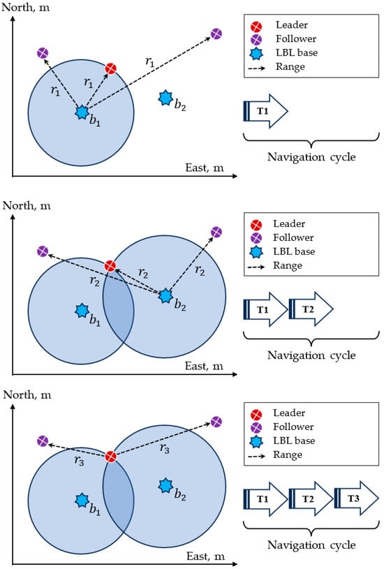
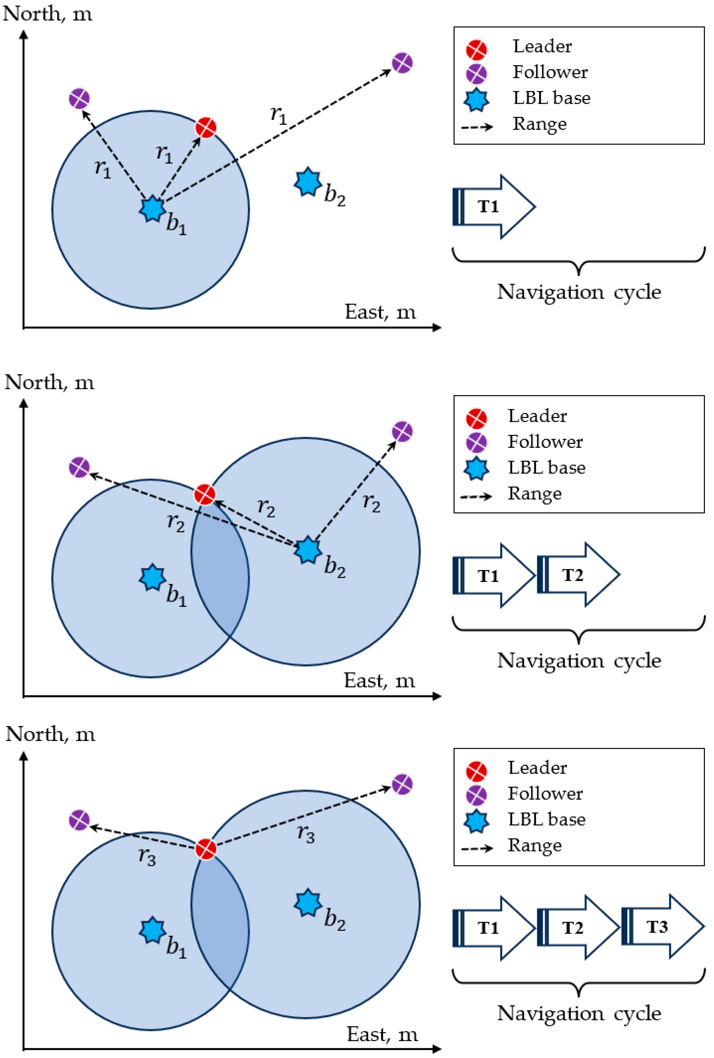
The proposed three-stage sparse LBL scheme assumes two fixed acoustic bases $b_1$ and $b_2$ and a group of $N$ underwater vehicles with a designated leader. Communication and ranging proceed through three one-way travel time (OWTT) stages: the first two are sequential broadcasts from $b_1$ and $b_2$ carrying identifiers and emission timestamps; the third is a broadcast from the leader. Each vehicle timestamps the receptions from $b_1$ and $b_2$ and forms slant ranges $r_1$ and $r_2$ (Figure 1). With measured depth (pressure) and a calibrated sound-speed profile $c\left(z\right)$, localization reduces to a constrained trilateration problem: in a horizontal plane with fixed depth, the position is determined from the intersection of circles with radii $r_1$ and $r_2$; in 3D, depth provides an additional constraint to intersect spheres.

Figure 1. Leader–follower navigation scheme.

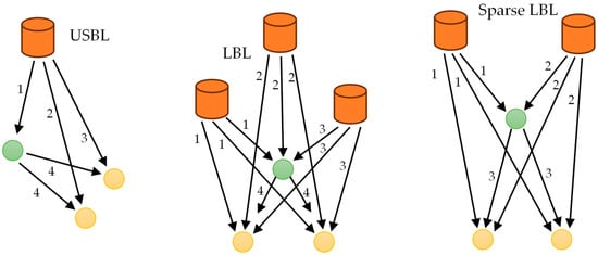
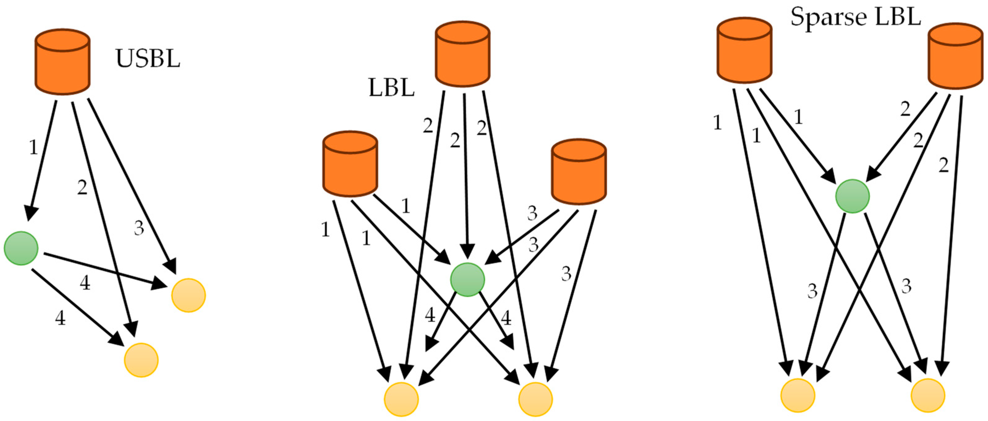
Let $\tau$ denote the stage duration, including payload, guard time, and the worst-case propagation $R_{max}/c$ ($R_{max}$—maximum operating range). The duration of a complete navigation–control cycle then depends on the acoustic infrastructure and scheduling policy. In a single-base USBL system operating by polling, the delivery of navigation data to $N$ vehicles requires $N$ individual stages plus one broadcast stage from the leader, so $(N+1)\tau$. In a classical three-base LBL system, three broadcasts provide simultaneous ranging to all vehicles and one additional stage carries the leader’s broadcast, giving $4\tau$. In the proposed two-base, three-stage scheme, two broadcasts from the bases suffice for ranging and the third stage serves the leader’s downlink, yielding $3\tau$. The cycle time thus becomes independent of $N$, in contrast to USBL polling, where it grows linearly with the group size. Relative to three-base LBL, the cycle is shorter by 25% (from $4\tau$ to $3\tau$) while also reducing infrastructure and channel occupancy.

This structure is well aligned with leader–follower coordination under OWTT. The first two stages create navigation observables for the entire formation concurrently, providing inherent scalability without increasing cycle time and reducing the probability of channel collisions. The third stage offers a deterministic downlink from the leader, ensuring timely dissemination of trajectory updates, role assignments, formation parameters, and navigation aids such as clock-drift estimates, sound-speed corrections, and integrity indicators. The fixed latency $3\tau$ stabilizes the formation-level control period, which benefits trajectory-tracking accuracy. By contrast, USBL polling introduces latency and jitter that increase with $N$, degrading synchronization among followers (Figure 2).

Figure 2. Leader–follower navigation comparison.

Observability with two ranges is addressed explicitly. In a planar setting, two circle intersections may arise; ambiguity is resolved by estimator continuity (predict–update consistency), appropriate baseline geometry, and, when needed, by leader broadcast disambiguation cues (e.g., admissible region flags). If one base transmission is missed, the estimator performs a partial update with a single range and inertial prediction until the next full cycle; in USBL polling, a comparable miss typically postpones that vehicle’s update by at least one entire polling cycle. Time synchronization requirements remain moderate: OWTT relies on known emission times and bounded clock error.

The same three-stage design is not generally suitable for other group topologies. Decentralized consensus, virtual-structure, or fully behavior-based formations distribute authority and typically rely on peer-to-peer exchanges, multi-leader/hierarchical signaling, or iterative agreement protocols; these patterns require additional uplink/downlink opportunities or event-triggered interactions that break the fixed three-stage schedule. Moreover, when formation management hinges on reciprocal relative measurements or on robustness to leader loss, the communication graph departs from a star centered on the leader, and the single dedicated downlink becomes insufficient to sustain coordination without added slots. Contemporary reviews document these trade-offs across architectures—advantages of simplicity and implementability for leader–follower versus vulnerabilities to leader failures and communication faults—underscoring that the proposed schedule is purpose-built for synchronous leader–follower formations and should not be generalized to topologies whose information flow is inherently multi-hop or symmetric [18].

In summary, the three-stage, two-base method achieves an $N$-independent update time, reduces acoustic channel load, and embeds a dedicated coordination downlink, thereby maintaining high inter-vehicle consistency with minimal equipment on followers. These properties make the approach particularly suitable for leader–follower missions—formation keeping, convoying, and search-and-track—where deterministic latency and scalable one-way communication are critical.

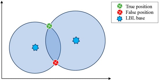
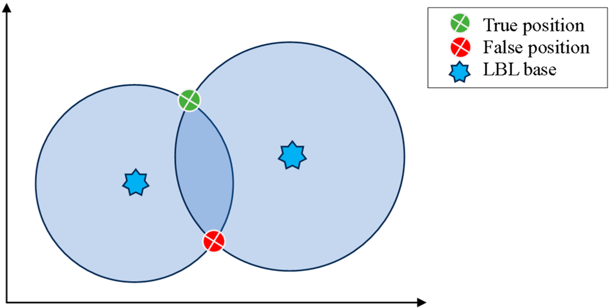
A further subtlety of sparse LBL with two transponders is the geometric duality of the range solution (Figure 3). With two slant ranges, the locus of feasible vehicle positions in 3D is the intersection of two spheres, i.e., a circle. If the vehicle depth is known (from a pressure sensor) or constrained, the problem reduces to two intersections of circles in the horizontal plane—two symmetric candidates reflected about the baseline connecting the transponders. This ambiguity can be removed either geometrically, by restricting the operational half-plane relative to the baseline, or statistically, by fusing kinematics/dynamics in a state estimator that selects the candidate consistent with the prediction.

Figure 3. Sparse LBL problem.

In operational terms, sparse LBL with two bases therefore exhibits a deterministic timing advantage but introduces a binary geometric ambiguity that is benign when the operational half-plane is fixed, and otherwise is cleanly resolved by model-based estimation. Depth aiding is pivotal: when depth is unknown, two slant ranges define a circle of solutions in 3D; a single depth measurement collapses this circle to the two explicit candidates given above.

The two intersection candidates are obtained from the classical circle–circle geometry in the horizontal plane. Let the transponder coordinates be $b_i={\left[\begin{array}{ccc}{x}_i& y_i& z_i\end{array}\right]}^T$, where $i=1,2$ and let the effective horizontal radii, corrected for the known target’s depth $z$, be

$${\rho }_i^{\perp }=\sqrt{\max \left\{r_i^2-{\left(z-z_i\right)}^2, 0\right\}}, i=\mathrm{1,2},$$

(1)

with $z_i$ denoting the depths of the bases and $r_i$ the measured slant ranges, which are calculated in a well-known way based on the signal’s flight time $t_i^{\mathrm{O}\mathrm{W}\mathrm{T}\mathrm{T}}=t-t_i$ ($t_i$—signal’s sending time) and the acoustic signal propagation profile $c\left(z\right)$ [30].

$$r_i={\displaystyle \frac{c\left(z\right)}{t_i^{\mathrm{O}\mathrm{W}\mathrm{T}\mathrm{T}}}}.$$

(2)

Define the displacement vector and its norm:

$$∆x=x_2-x_1, ∆y=y_2-y_1, d=\sqrt{∆x^2+∆y^2}.$$

(3)

The scalar distance from $b_1$ to the line of intersection is then

$$a={\displaystyle \frac{{\left({\rho }_1^{\perp }\right)}^2-{\left({\rho }_2^{\perp }\right)}^2+d^2}{2d}}$$

(4)

and the half-chord length orthogonal to this line is

$$h=\sqrt{{\left({\rho }_1^{\perp }\right)}^2-a^2}.$$

(5)

The midpoint on the line between the two circle centers is

$$x_m=x_1+a{\displaystyle \frac{∆x}{d}}, y_m=y_1+a{\displaystyle \frac{∆y}{d}}.$$

(6)

Finally, the two possible intersection coordinates in three dimensions are obtained as

$$x=x_m\pm h{\displaystyle \frac{∆y}{d}}, y=y_m\mp h{\displaystyle \frac{∆x}{d}}.$$

(7)

The existence of two symmetric candidates in the horizontal plane, obtained from the intersection of depth-aided circles, creates a fundamental challenge for sparse two-base localization.

One possible solution to the given challenges is the Kalman estimator. This approach has been referenced in [1,2] and in proprietary closed-source solutions [3]. The considered open solutions did not examine the accurate object dynamics model, and did not handle the two-unit base scenario.

Reliable position estimation using Kalman approaches from two slant ranges becomes feasible once the ranges $r_i$ are included as augmented states and explicitly coupled to the vehicle kinematics. Let the vehicle position be ${\eta }_1={\left[\begin{array}{ccc}x& y& z\end{array}\right]}^T$, the Euler angles ${\eta }_2={\left[\begin{array}{ccc}\phi & \theta & \psi \end{array}\right]}^T$, the body-fixed linear velocity ${\nu }_1={\left[\begin{array}{ccc}u& v& w\end{array}\right]}^T$ and the body-fixed angular velocity ${\nu }_2={\left[\begin{array}{ccc}p& q& r\end{array}\right]}^T$. Then, the augmented state vector results in

$$\mathbb{x}={\left[\begin{array}{ccc}\left[\begin{array}{cc}{\eta }_1^T& {\eta }_2^T\end{array}\right]& \left[\begin{array}{cc}{\nu }_1^T& {\nu }_2^T\end{array}\right]& \left[\begin{array}{cc}{r}_1& r_2\end{array}\right]\end{array}\right]}^T.$$

(8)

For acoustic bases at $b_i$ define $r_i=\Vert {\eta }_1-b_i\Vert$. Differentiation gives the continuous-time range dynamics [31]:

$${\dot{r}}_i={\displaystyle \frac{{\left({\eta }_1-b_i\right)}^T\left({\dot{\eta }}_1-{\dot{b}}_i\right)}{r_i}},$$

(9)

where ${\dot{b}}_i\approx 0$ in the quasi-stationary operating mode consideration and the inertial linear velocity ${\dot{\eta }}_1={\left[\begin{array}{ccc}\dot{x}& \dot{y}& \dot{z}\end{array}\right]}^T$ is obtained from the SNAME rotation matrix:

$$\begin{array}{c}{\dot{\eta }}_1=R_I^B{\left({\eta }_2\right)}^{-1}{\nu }_1\\ =\\ {\left[\begin{array}{ccc}\cos \psi \cos \theta & \sin \psi \cos \theta & -\sin \theta \\ -\sin \psi \cos \phi +\cos \psi \sin \theta \sin \phi & \cos \psi \cos \phi +\sin \psi \sin \theta \sin \phi & \sin \phi \cos \theta \\ \sin \psi \sin \phi +\cos \psi \sin \theta \cos \phi & -\cos \psi \sin \phi +\sin \psi \sin \theta \cos \phi & \cos \phi \cos \theta \end{array}\right]}^{-1}{\nu }_1\end{array}.$$

(10)

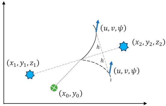
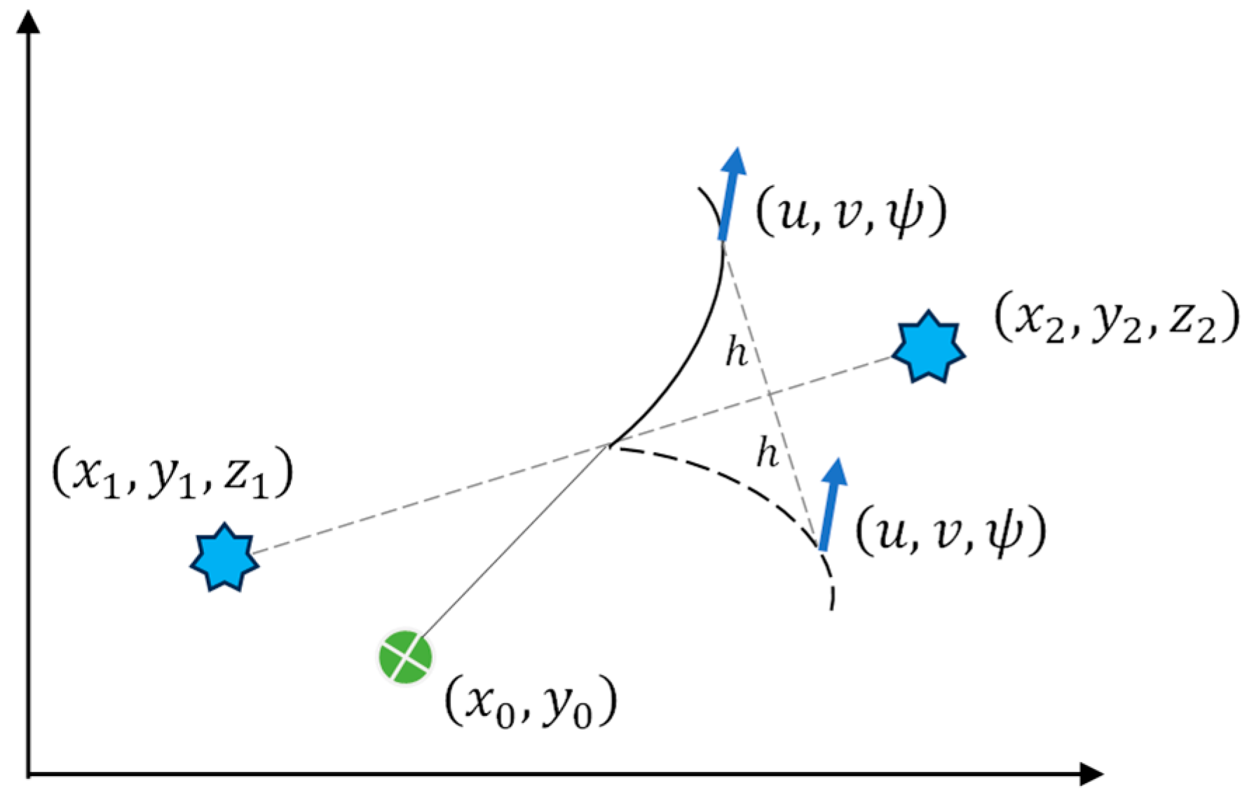
At any fixed instant, the depth-aided circle–circle construction (7) admits two mirror-symmetric horizontal candidates $(x^{\pm },y^{\pm })$ that share the same pair $(r_1,r_2)$. Their temporal evolution of ranges is, however, generically different. The associated line-of-sight unit vectors to each base differ by the sign of their horizontal cross-track component with respect to the baseline of the two bases; hence, unless the inertial cross-track component of the vehicle velocity is exactly zero, the pair of range rates $({\dot{r}}_1,{\dot{r}}_2)$ computed via (9) cannot simultaneously match both candidates. A Kalman-type estimator that propagates the augmented $(r_1,r_2)$ via the range-rate kinematics (9)–(10), driven by the available aiding information (e.g., depth, attitude, velocity), and corrects with discrete measured ranges $\mathbb{y}={\left[\begin{array}{ccc}\dots & {\tilde{r}}_1& {\tilde{r}}_2\end{array}\right]}^T$ enforces the temporal (dynamic) consistency of the ranges; the signed innovations remain small only on the dynamically consistent branch, and the estimate converges to the correct position without any discontinuous branch switching. In weak geometry (small half-chord $h$) or nearly parallel motion to the baseline, discrimination weakens and convergence may slow, but resumes once nonzero cross-track motion or mild maneuvering reappears (Figure 4).

Figure 4. Baseline crossing problem.

When at least three independent slant ranges to non-collinear transponders are available and depth is aided, the horizontal position $(x, y)$ becomes uniquely determined (no binary symmetry). In this regime, a standard Kalman-type estimator that uses the vehicle kinematics and the range measurement model suffices; no branch-selection heuristics are required. In the present architecture, followers have access to three ranges, whereas the leader currently receives only two; hence, the disambiguation machinery is only needed on the leader.

The augmented state vector in three slant ranges will take the following form:

$$\mathbb{x}={\left[\begin{array}{ccc}\left[\begin{array}{cc}{\eta }_1^T& {\eta }_2^T\end{array}\right]& \left[\begin{array}{cc}{\nu }_1^T& {\nu }_2^T\end{array}\right]& \left[\begin{array}{ccc}{r}_1& r_2& r_3\end{array}\right]\end{array}\right]}^T,$$

(11)

where $r_3$ is obtained by substituting the leader’s ${\eta }_1$ and ${\dot{\eta }}_1$ into (9) instead of $b_3$ and ${\dot{b}}_3$, respectively.

Although augmenting $r_i$ resolves the ambiguity in principle, convergence can be slow under weak geometry, poor initialization, or sparse OWTT updates. In practice, faster and more robust convergence is obtained by adding light pseudo-measurements consistent with (7) and (9) (e.g., depth aiding and horizontal branch-consistency residuals) whose weights are reduced adaptively as $h\to 0$.

In many operational deployments, the initial horizontal location $\left(x_0,y_0\right)$ is poorly constrained, while initial ranges are determined as $r_{i,0}=\Vert {\eta }_{\mathrm{1,0}}-b_{i,0}\Vert$. Under such conditions the dominant uncertainty lies in the cross-track direction with respect to the transponder baseline, whereas the along-track component is comparatively better constrained.

A practical and principled means to accelerate convergence is diffuse initialization of the Kalman-type estimator [32,33]. Conceptually, “diffuse” means that the variance in the weak (cross-track) direction is taken to be arbitrarily large; in implementation, large but finite values are used to preserve numerical stability. In Cartesian coordinates this amounts to inflating the diagonal entries $P_0\left(x,x\right)$ and $P_0\left(y,y\right)$. No artificial “infinite” off-diagonal term $P_0\left(x,y\right)=P_0\left(y,x\right)$ is required. The remaining priors (depth, attitude, linear and angular velocities, ranges) follow sensor quality without artificial inflation.

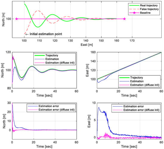
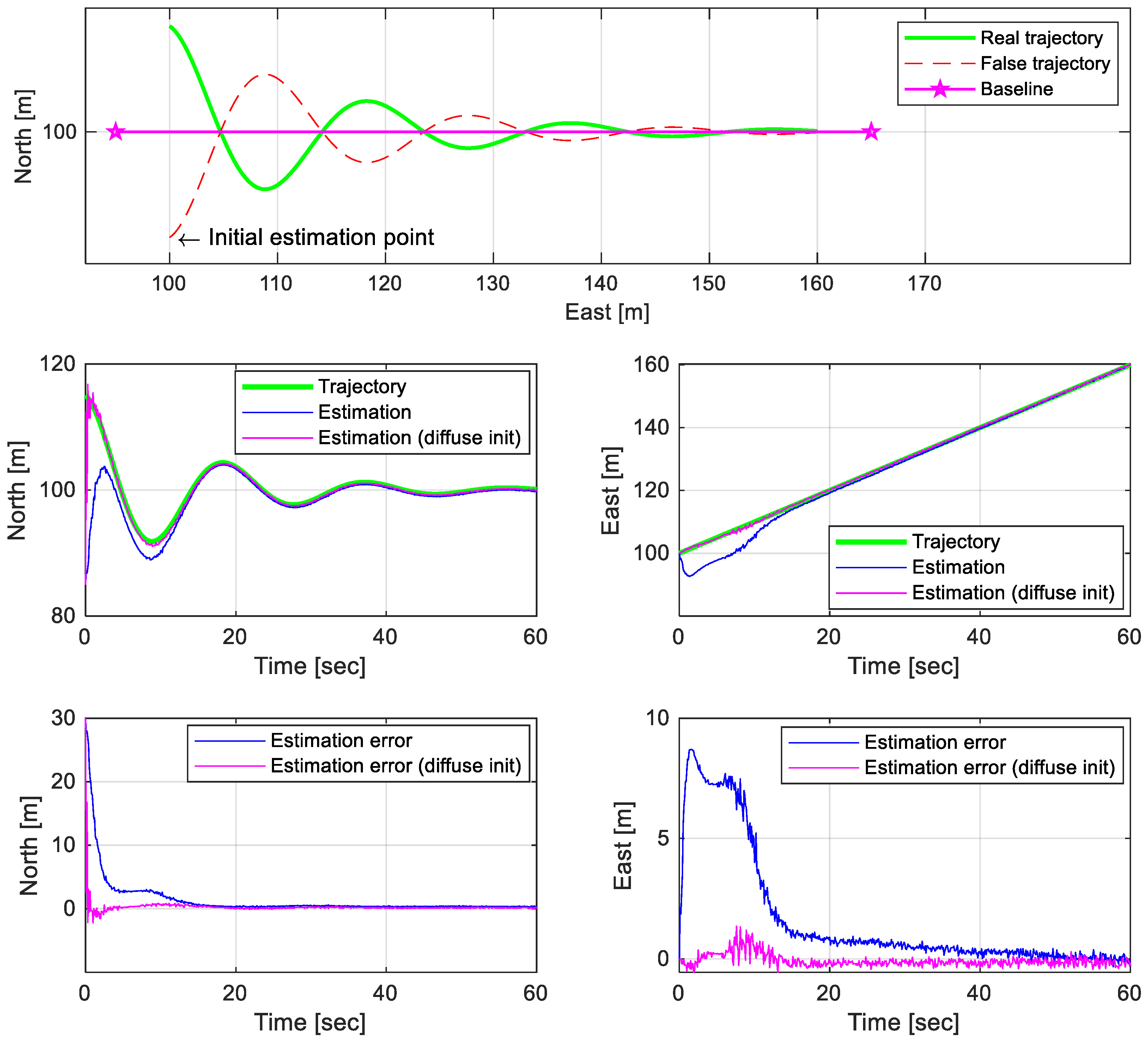
The accompanying Figure 5 illustrates the effect. Two mirror-symmetric candidate trajectories are plotted as a damped “snake” about the baseline. The initial estimate is deliberately placed on the wrong side. With a diffuse $P_0\left(x,x\right)\gg 1$, the estimator migrates to the dynamically consistent branch within a short transient, even with sparse OWTT updates. Small early discontinuities in the estimate appear at the start. After this transient, the trajectory settles and follows the intended path with bounded residuals.

Figure 5. Diffused initialization example.

If the vehicle moves strictly parallel to the baseline, cross-track excitation is minimal and the temporal information carried by the range evolution weakens. Convergence remains possible but occurs more slowly and benefits from occasional mild maneuvers that restore cross-track excitation. If the vehicle crosses the baseline nearly perpendicularly, the geometry is locally weak at the crossing but improves immediately afterward as the half-chord grows. The diffuse cross-track prior then allows the estimator to select the correct side promptly once the geometry strengthens.

The accuracy of time synchronization is a key factor determining the reliability of range estimation in navigation systems based on the one-way travel time measurement principle. In such systems, the distance $r_i$ between the transmitting (remote) and receiving (host) nodes is computed according to (2), where $t_i^{\mathrm{O}\mathrm{W}\mathrm{T}\mathrm{T}}$ denotes the difference between the local timestamps of signal transmission and reception. Any offset or instability of the local time bases directly leads to a metric error in the estimated range.

This error primarily arises from the limited precision and stability of the time sources used. High-precision reference oscillators such as atomic clocks (rubidium or cesium) provide frequency stability better than ${10}^{-11}$–${10}^{-12}$; however, their application is constrained by cost, size, and power consumption. More practical alternatives include temperature-compensated crystal oscillators (TCXOs) and oven-controlled crystal oscillators (OCXOs), which typically achieve stabilities of ${10}^{-8}$–${10}^{-9}$ and ${10}^{-7}$–${10}^{-8}$, respectively. These oscillators can be integrated with microcontroller-based systems and are often used in acoustic transponders and distributed in underwater navigation units. The built-in crystal oscillators of general-purpose microcontrollers (e.g., STM32) have typical stabilities of 20–50 ppm, corresponding to timing errors of several tens of microseconds per second of free running.

Consider first the case of ideal frequency stability ($\mathrm{p}\mathrm{p}\mathrm{m}=0$), when no drift of the time base occurs and the error is caused solely by the finite temporal resolution of the local clock, characterized by the discretization step $\delta t$. During time measurement, the value is truncated to the admissible step:

$${\tilde{t}}_i^{\mathrm{O}\mathrm{W}\mathrm{T}\mathrm{T}}={\displaystyle \frac{\mathrm{fix}\left(t_i^{\mathrm{O}\mathrm{W}\mathrm{T}\mathrm{T}}·{10}^d\right)}{{10}^d}},$$

(12)

where $d$ defines the number of significant digits corresponding to the desired clock resolution. The resulting range calculation error can be expressed as

$$∆r_i=\left|r_i-c·{\tilde{t}}_i^{\mathrm{O}\mathrm{W}\mathrm{T}\mathrm{T}}\right|=c\left|t_i^{\mathrm{O}\mathrm{W}\mathrm{T}\mathrm{T}}·{\tilde{t}}_i^{\mathrm{O}\mathrm{W}\mathrm{T}\mathrm{T}}\right|.$$

(13)

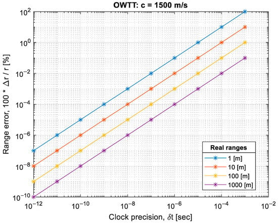
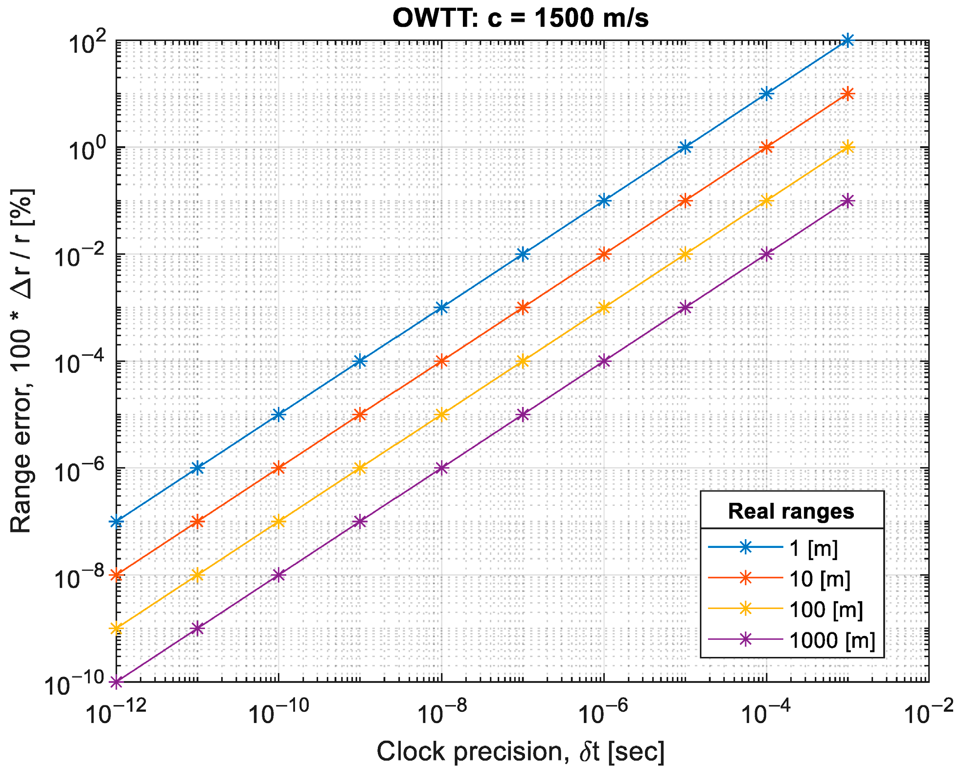
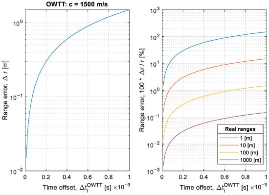
With a constant sound speed, the absolute range error increases with the growth of the clock quantization step $\delta t$. Figure 6 illustrates that as the inaccuracy of the time interval ${\tilde{t}}_i^{\mathrm{O}\mathrm{W}\mathrm{T}\mathrm{T}}$ increases, the absolute error of the range estimation also grows, assuming a constant sound-speed value in water of $c\left(z\right)~1500$ and the idealized clock resolution.

Figure 6. Range calculation error.

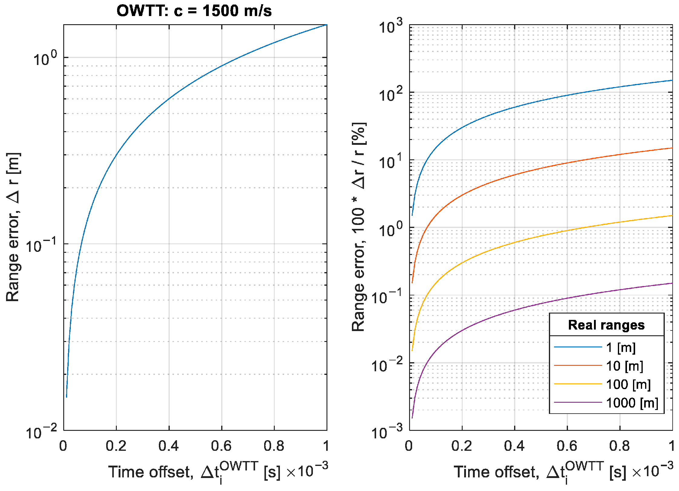
Next, consider the influence of a time base offset between the host and remote nodes under the assumption of ideal temporal resolution. Let the true travel time of the signal be $t_i^{\mathrm{O}\mathrm{W}\mathrm{T}\mathrm{T}}$, and let the offset between the local clocks be denoted as $∆t_i^{\mathrm{O}\mathrm{W}\mathrm{T}\mathrm{T}}$. In this case, the estimated range error is determined as

$$∆r_i=\left|r_i-c\left(t_i^{\mathrm{O}\mathrm{W}\mathrm{T}\mathrm{T}}+∆t_i^{\mathrm{O}\mathrm{W}\mathrm{T}\mathrm{T}}\right)\right|=c·∆t_i^{\mathrm{O}\mathrm{W}\mathrm{T}\mathrm{T}}.$$

(14)

As the time offset between nodes increases, the range estimation error grows linearly, even when the clock resolution is ideal. Figure 7 demonstrates that an increase in the temporal misalignment between the host and remote devices results in a proportional increase in OWTT-based range errors.

Figure 7. Range calculation error.

Analysis of these dependencies shows that for microcontroller-based systems with high-stability crystal oscillators, microsecond-level timing precision is sufficient for most practical applications. Such precision ensures range errors on the centimeters order, comparable to uncertainties arising from sound-speed variability and multipath effects in the aquatic environment. The use of TCXOs or OCXOs in combination with low-cost microcontrollers (e.g., STM32) provides a rational compromise between cost, energy efficiency, and the metrological requirements of OWTT-based navigation systems.

The complete range estimation formula, considering the above factors, can be written as follows:

$${\tilde{r}}_i=c·{\tilde{t}}_i^{\mathrm{O}\mathrm{W}\mathrm{T}\mathrm{T}}=c{\displaystyle \frac{\mathrm{fix}\left(\left(t_i^{\mathrm{O}\mathrm{W}\mathrm{T}\mathrm{T}}+∆t_i^{\mathrm{O}\mathrm{W}\mathrm{T}\mathrm{T}}\right)·{10}^d\right)}{{10}^d}}.$$

(15)

It should be emphasized that the factors considered here—clock quantization and temporal offset—are not the only sources of measurement error. Additional uncertainties stem from temperature and salinity variations that affect the local sound-speed profile, as well as from transmission delays and hardware-specific timestamping effects. Nevertheless, the accuracy of time interval measurement and the stability of local oscillators define the fundamental limits of positioning precision in systems employing the OWTT method.

To ensure stable and reproducible timing within embedded OWTT-based navigation units, a dedicated hardware time base was developed using a microcontroller with an external high-stability crystal oscillator. The oscillator provides the reference frequency ${\mathrm{F}}_{\mathrm{X}\mathrm{O}}$ and can be implemented either as a temperature-compensated crystal oscillator (TCXO) or an oven-controlled crystal oscillator (OCXO), depending on the required frequency stability and environmental conditions. Using such oscillators as external references enables precise timing without the complexity or cost associated with atomic standards.

The proposed implementation is based on the STM32 (STMicroelectronics, Plan-les-Ouates, Switzerland) microcontroller family, which offers an advantageous combination of features for this task: hardware timers with external clocking capability, low jitter, high internal bus frequency, and wide peripheral support. STM32 microcontrollers provide direct access to the timer’s external trigger input (TIMx_ETR), allowing the oscillator signal to be fed directly into the timer without intermediate conditioning circuits. This configuration ensures accurate counting of oscillator pulses in hardware while minimizing CPU overhead and interrupt latency.

Let ${\mathrm{F}}_{\mathrm{X}\mathrm{O}}$ denote the oscillator frequency (Hz), and let $\mathrm{D}\mathrm{I}\mathrm{V}$ represent the total division factor between the oscillator signal and the timer counter (including all hardware prescalers). The auto-reload register value is $\mathrm{A}\mathrm{R}\mathrm{R}$, the current counter value is $\mathrm{C}\mathrm{N}\mathrm{T}$, and ${\mathrm{N}}_{\mathrm{I}\mathrm{N}\mathrm{T}}$ denotes the accumulated number of timer update (overflow) events tracked in software. The local time $t$ (in seconds) is determined from the expression

$$t={\displaystyle \frac{\mathrm{D}\mathrm{I}\mathrm{V}\times \left[{\mathrm{N}}_{\mathrm{I}\mathrm{N}\mathrm{T}}\left(\mathrm{A}\mathrm{R}\mathrm{R}+1\right)+\mathrm{C}\mathrm{N}\mathrm{T}\right]}{{\mathrm{F}}_{\mathrm{X}\mathrm{O}}}},$$

(16)

where $\mathrm{D}\mathrm{I}\mathrm{V}$ accounts for all effective prescaling stages of the timer. The formula is applicable to both 16-bit and 32-bit STM32 timers and ensures consistent timestamp reconstruction from the hardware counter.

This configuration allows the STM32 timer to generate timestamps with a microsecond resolution, which is sufficient for the underwater navigation applications considered in this work. The external crystal oscillator defines the long-term stability of the time base (typically better than 0.1 ppm for TCXO or OCXO), while the timer hardware provides high short-term precision and immunity to software latency. As a result, this implementation offers an optimal balance between accuracy, complexity, and energy efficiency, making it a practical and reliable solution for distributed OWTT-based navigation systems.

2.2. State Estimation

Control systems containing two measurement channels (continuous and discrete) are characterized by the same formalized representation of physical processes occurring in the loop.

The system dynamics model is represented by an interrelated system of ordinary differential and finite-difference equations as follows:

$${\displaystyle \genfrac{}{}{0pt}{}{\frac{d\mathbb{x}\left(t\right)}{dt}=A_1\left(t\right)\mathbb{x}\left(t\right)+B_1\left(t\right)u_1\left(t\right)+{\mathcal{w}}_1\left(t\right), t\in T_i,}{\begin{array}{c}x\left(t_{i+1}\right)=A_2\left(t_i\right)x\left(t_i\right)+B_2\left(t_i\right)u_2\left(t_i\right)+{\mathcal{w}}_2\left(t_i\right), t_i\in \mathsf{\Theta },\\ x\left(t_0\right)={\mathbb{x}}_0.\end{array}}}$$

(17)

In Equation (17) the following notations are assumed: $T_i=[t_i,t_{i+1})$—semi-open control system time interval between the discrete subsystem operation moments, $T=\left[t_0,t_f\right]$—total system uptime, $t_0$ and $t_f$ are the initial and final control process time moments, respectively, $\mathsf{\Theta }=\left\{t_1,t_2,\dots ,t_{k_f}:\left(t_{i+1}-t_i\right)>0\right\}$—discrete subsystem functioning moments set, $\mathbb{x}\in R^n$—state vector whose elements are continuously differentiable functions on $T_i$ and tolerate the first kind of discontinuities on $\mathsf{\Theta }$, and the right limits are taken as the vector $\mathbb{x}$ element values at the discontinuity points, $u_1\in R^{m_1}$, $u_2\in R^{m_2}$—control vectors of the continuous and discrete subsystems, respectively, ${\mathcal{w}}_1$ and ${\mathcal{w}}_2$—$n$-dimensional disturbance vectors, ${\mathbb{x}}_0$—initial state vector.

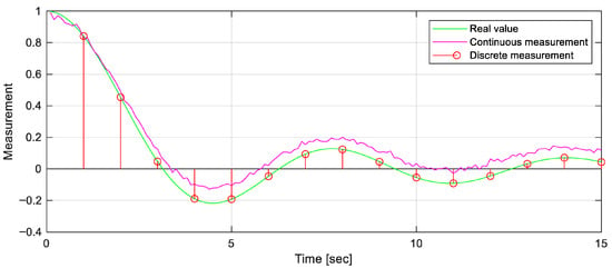
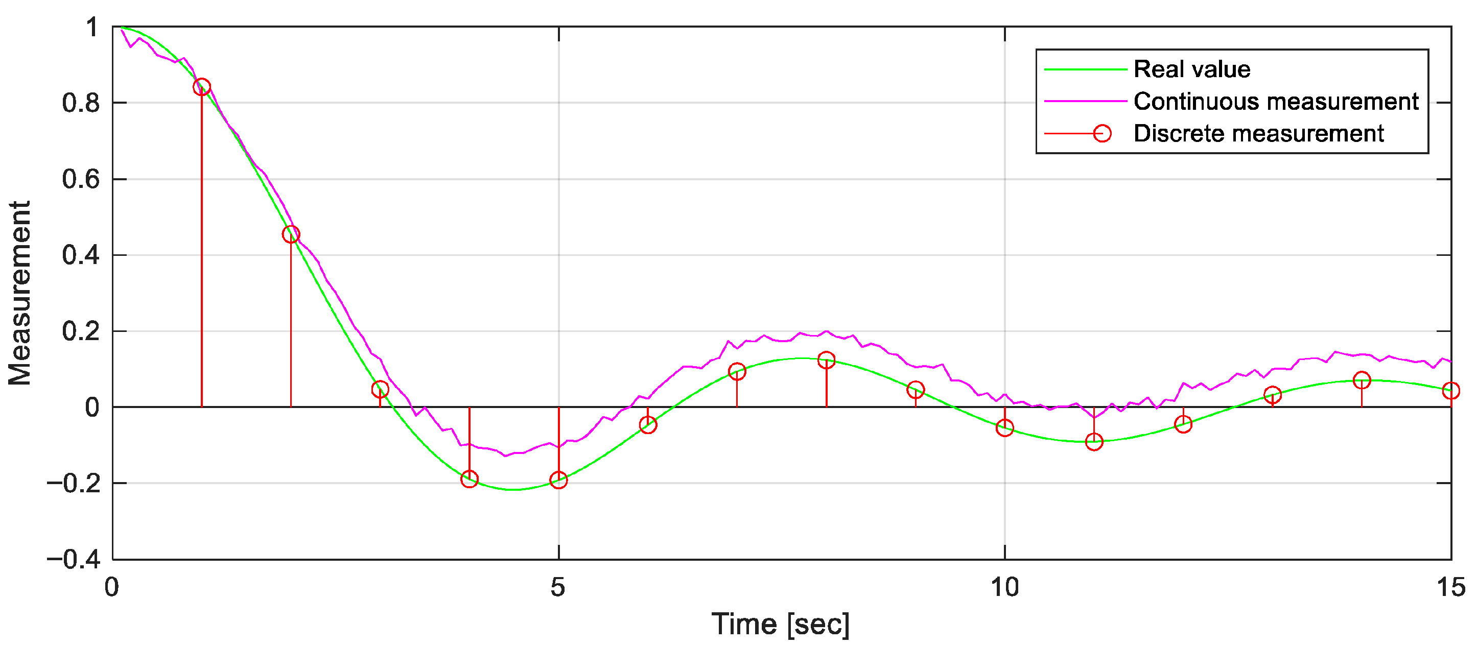
The control system contains continuous and discrete measurement devices (Figure 8) functioning in accordance with the following equations:

$${\displaystyle \genfrac{}{}{0pt}{}{{\mathbb{y}}_1\left(t\right)=C_1\left(t\right)\mathbb{x}\left(t\right)+{\mathcal{v}}_1\left(t\right), t\in T_i,}{{\mathbb{y}}_2\left(t_i\right)=C_2\left(t_i\right)\mathbb{x}\left(t_i\right)+{\mathcal{v}}_2\left(t_i\right), t_i\in \mathsf{\Theta },}}$$

(18)

where ${\mathbb{y}}_1\left(t\right)$ and ${\mathbb{y}}_2\left(t_i\right)$—$q_1$- and $q_2$-dimensional continuous and discrete measurement vectors, ${\mathcal{v}}_1\left(t\right)$ and ${\mathcal{v}}_2\left(t_i\right)$—measurement noise vectors.

Figure 8. Discrete–continuous measurements.

The matrices $A_1$, $B_1$, $C_1$ and $A_2$, $B_2$, $C_2$ respectively consist of piecewise continuous and piecewise constant elements and agree with (17) and (18). Then, the optimal non-stationary continuous–discrete filter equations will have the form

$${\displaystyle \genfrac{}{}{0pt}{}{\mathcal{A}\widehat{\mathbb{x}}\left(t\right)=K\left(t\right)\left[{\mathbb{y}}_1\left(t\right)-C_1\left(t\right)\widehat{\mathbb{x}}\left(t\right)\right], t\in T_i,}{\begin{array}{c}A\widehat{\mathbb{x}}\left(t_i\right)=K\left(t_i\right)\left[{\mathbb{y}}_2\left(t_i\right)-C_2\left(t_i\right)A_2\left(t_i\right)\widehat{\mathbb{x}}\left(t_{i-1}\right)\right], t_i\in \mathsf{\Theta },\\ x\left(t_0\right)=0.\end{array}}}$$

(19)

The equations for the matrix filter gains are written in the form

$${\displaystyle \genfrac{}{}{0pt}{}{K\left(t\right)=P\left(t\right)C_1^T\left(t\right)R_1^{-1}\left(t\right), t\in T_i,}{K\left(t_i\right)=P_1\left(t_i\right)C_2^T\left(t_i\right){\left[C_2\left(t_i\right)P_1\left(t_i\right)+R_2\left(t_i\right)\right]}^{-1}, t_i\in \mathsf{\Theta },}}$$

(20)

and the covariance matrix equation for the estimation error has the following form:

$$\begin{array}{c}{\displaystyle \genfrac{}{}{0pt}{}{\frac{dP\left(t\right)}{dt}=A_1\left(t\right)P\left(t\right)+P\left(t\right)A_1^T\left(t\right)+B_1\left(t\right)Q_1\left(t\right)B_1^T\left(t\right)-P\left(t\right)C_1^T\left(t\right)R_1^{-1}\left(t\right)C_1\left(t\right)P\left(t\right), t\in T_i,}{P\left(t_{i-1}\right)=P_1\left(t_i\right)-P_1\left(t_i\right)C_2^T\left(t_i\right){\left[C_2\left(t_i\right)P_1\left(t_i\right)C_2^T\left(t_i\right)+R_2\left(t_i\right)\right]}^{-1}{C}_2\left(t_i\right)P_1\left(t_i\right), t_i\in \mathsf{\Theta },}}\\ P_1\left(t_i\right)=A_2\left(t_i\right)P\left(t_{i-1}\right)A_2^T\left(t_i\right)+B_2\left(t_i\right)Q_2\left(t_i\right)B_2^T\left(t_i\right),\\ P\left(t_0\right)=P_0.\end{array}$$

(21)

The present paper proposes discrete and continuous channel fusion by solving the continuous component to estimate (19) at each discrete time interval $\left[t_i, t_{i+1}\right]\in \mathsf{\Theta }$.

The initial conditions $\mathbb{x}\left(0\right)=\mathbb{x}\left(t_i\right)$ are equal to the discrete filter estimate $\widehat{\mathbb{x}}\left(t_i\right)$, which is assumed to be more accurate but available at a lower rate.

Estimating hydrodynamic parameters is crucial for improving the state estimation convergence by reducing model uncertainties. Accurate hydrodynamic models enhance the leader’s dynamics prediction for more reliable navigation and control in complex underwater environments [28]. This is particularly important for autonomous operations where unmodeled hydrodynamic effects can significantly degrade estimation accuracy.

To begin with, assume the state vector assembly without augment components. General coordinates of an autonomous underwater vehicle (AUV) are determined in a geocentric coordinate system using SNAME notation [34]:

$$\eta =\left[\begin{array}{c}{\eta }_1\\ {\eta }_2\end{array}\right]\in {\mathbb{R}}^6,$$

(22)

where ${\eta }_1={\left[\begin{array}{ccc}x& y& z\end{array}\right]}^T$ determines the longitudinal, lateral, and vertical positions, respectively, and the vector ${\eta }_2={\left[\begin{array}{ccc}\phi & \theta & \psi \end{array}\right]}^T$ determines the Euler angles: roll, pitch, and yaw, respectively.

The velocity vector $\mathsf{\nu }$ is expressed in the body-fixed frame [34]. The velocities (linear and angular) according to the notation announced above should be written as

$$\nu =\left[\begin{array}{c}{\nu }_1\\ {\nu }_2\end{array}\right]={\left[\begin{array}{cccccc}u& v& w& p& q& r\end{array}\right]}^T.$$

(23)

Under the influence of hydrodynamic effects caused by the environment, the underwater vehicle dynamics can be expressed as

$$\begin{array}{c}M\dot{\nu }+C\left(\nu \right)\nu +D\left(\nu \right)\nu +g\left(\eta \right)=\tau +J^T\left(\eta \right){\bar{f}}_e,\\ M=M_{RB}+M_A,\\ C\left(\nu \right)=C_{RB}\left(\nu \right)+C_A\left(\nu \right),\end{array}$$

(24)

where $M_{RB}\in {\mathbb{R}}^{n\times n}$—rigid body inertia matrix ($n$ is the DoF number);

$M_A\in {\mathbb{R}}^{n\times n}$—added mass matrix;

$C_{RB}\left(\mathsf{\nu }\right)\in {\mathbb{R}}^{n\times n}$—rigid body Coriolis matrix;

$C_A\left(\mathsf{\nu }\right)\in {\mathbb{R}}^{n\times n}$—added mass Coriolis matrix;

$D\left(\mathsf{\nu }\right)\in {\mathbb{R}}^{n\times n}$—damping matrix;

$g\left(\eta \right)\in {\mathbb{R}}^{n\times 1}$—gravitational forces and moments vector;

$\tau \in {\mathbb{R}}^{n\times 1}$—vector (of forces and moments) of the controls applied to the body expressed in the body-fixed frame;

${\bar{f}}_e\in {\mathbb{R}}^{n\times 1}$—vector (of forces and moments) of general external disturbance applied to the body expressed in the inertial frame which may include current-induced effects, unmodeled hydrodynamic terms, and other exogenous perturbations.

The kinematics equation linking (22) and (23) is written in the form

$$\dot{\eta }=J^{-1}\left(\eta \right)\nu ={\left[\begin{array}{cc}{R}_I^B\left(\eta \right)& 0_{3\times 3}\\ 0_{3\times 3}& J_{k,o}\left(\eta \right)\end{array}\right]}^{-1}\nu =\left[\begin{array}{cc}{R}_B^I\left(\eta \right)& 0_{3\times 3}\\ 0_{3\times 3}& J_{k,o}^{-1}\left(\eta \right)\end{array}\right]\nu ,$$

(25)

where $R_I^B\left(\eta \right)\in {\mathbb{R}}^{3\times 3}$—the rotation matrix obtained from the Euler angles, which links the navigation (inertial) frame and the underwater vehicle (body) frame; ${\mathrm{J}}_{k,o}\left(\eta \right)\in {\mathbb{R}}^{3\times 3}$—the Jacobian linking the angular velocities of the world reference system and the body system [34].

Given ${\mathbb{x}}_{\left\{\mathrm{N}\mathrm{A}\right\}}=\left[\begin{array}{c}\eta \\ \nu \end{array}\right]$, it is possible to write the non-augmented state vector derivative:

$${\dot{\mathbb{x}}}_{\left\{\mathrm{N}\mathrm{A}\right\}}=\left[\begin{array}{c}\dot{\eta }\\ M^{-1}(\tau +J^T(\eta ){\bar{f}}_e-C(\nu )\nu -D(\nu )\nu -g(\eta \left)\right)\end{array}\right].$$

(26)

The latter equation can be represented in the SDC form:

$$\begin{gathered} {\dot{\mathbb{x}}}_{\left\{\mathrm{N}\mathrm{A}\right\}}=\mathit{A}\left({\mathbb{x}}_{\left\{\mathrm{N}\mathrm{A}\right\}},t\right){\mathbb{x}}_{\left\{\mathrm{N}\mathrm{A}\right\}}+\mathit{B}\left({\mathbb{x}}_{\left\{\mathrm{N}\mathrm{A}\right\}},t\right)\bar{u}, {\mathbb{x}}_{\left\{\mathrm{N}\mathrm{A}\right\}}\left(t_0\right)={\mathbb{x}}_{\left\{\mathrm{N}\mathrm{A}\right\}, 0}, \\ \mathbb{y}=\mathit{C}\left(t\right){\mathbb{x}}_{\left\{\mathrm{N}\mathrm{A}\right\}}+\mathit{D}\left(t\right)\bar{u}, \\ \mathit{A}\left({\mathbb{x}}_{\left\{\mathrm{N}\mathrm{A}\right\}},t\right){\mathbb{x}}_{\left\{\mathrm{N}\mathrm{A}\right\}}=\left[\begin{array}{cc}{0}_{6\times 6}& J({\mathbb{x}}_{\left\{\mathrm{N}\mathrm{A}\right\}}{)}^{-1}\\ 0_{6\times 6}& -M^{-1}\left(C\left({\mathbb{x}}_{\left\{\mathrm{N}\mathrm{A}\right\}}\right)+D\left({\mathbb{x}}_{\left\{\mathrm{N}\mathrm{A}\right\}}\right)\right)\end{array}\right], \mathit{B}\left({\mathbb{x}}_{\left\{\mathrm{N}\mathrm{A}\right\}},t\right)=\left[\begin{array}{c}{0}_{6\times 6}\\ M^{-1}\end{array}\right], \\ \bar{u}=\tau +u_{add}\left({\mathbb{x}}_{\left\{\mathrm{N}\mathrm{A}\right\}}\right),u_{add}=J^T\left({\mathbb{x}}_{\left\{\mathrm{N}\mathrm{A}\right\}}\right){\bar{f}}_e-g\left({\mathbb{x}}_{\left\{\mathrm{N}\mathrm{A}\right\}}\right), \end{gathered}$$

(27)

where $\mathit{A}\in {\mathbb{R}}^{2n\times 2n}$—dynamics matrix;

$\mathit{B}\in {\mathbb{R}}^{2n\times n}$—control matrix;

$\mathit{C}\in {\mathbb{R}}^{m\times 2n}$—output matrix ($m$—number of system outputs);

$\mathit{D}\in {\mathbb{R}}^{m\times n}$—input–output coupling matrix;

$\bar{u}\in {\mathbb{R}}^{n\times 1}$—control vector, including the vector of external perturbations $u_{add}\in {\mathbb{R}}^{n\times 1}$.

In this paper, a symmetric-body approximation is considered, which is standard for many AUV platforms with approximately port-starboard symmetry and body-fixed axes aligned with the principal directions. Under this assumption, the dominant added mass and hydrodynamic damping effects are primarily aligned with the surge/sway/heave and roll/pitch/yaw axes, while cross-coupling terms in $M_A$ and $D\left(\nu \right)$ are typically smaller and are neglected for modeling simplicity. Importantly, this choice also reduces the number of uncertain hydrodynamic coefficients that must be estimated in the augmented filter.

Given the symmetric form approximation of the underwater vehicle, the matrix notation is greatly simplified and becomes diagonal [35]:

$$M_A=-diag\left\{X_{\dot{u}}, Y_{\dot{v}}, Z_{\dot{w}}, K_{\dot{p}}, M_{\dot{q}}, N_{\dot{r}}\right\}.$$

(28)

Damping refers to velocity-dependent forces. The linear part $D_{LIN}$ consists of linear surface friction. The nonlinear damping $D_{NL}\left(\mathsf{\nu }\right)$ consists of all higher order terms such as turbulent skin-friction drag due to vortex shedding. In practice, the linear $D_{LIN}$ and quadratic $D_{QUAD}\left(\mathsf{\nu }\right)$ damping components are dominant [35]:

$$\begin{gathered} D\left(\mathsf{\nu }\right)=-diag\left\{X_u,Y_v,Z_w,K_p,M_q,N_r\right\} \\ -diag\left\{X_{u\left|u\right|}\left|u\right|,Y_{v\left|v\right|}\left|v\right|,Z_{w\left|w\right|}\left|w\right|,K_{p\left|p\right|}\left|p\right|,M_{q\left|q\right|}\left|q\right|,N_{r\left|r\right|}\left|r\right|\right\}=D_{LIN}+D_{QUAD}\left(\mathsf{\nu }\right). \end{gathered}$$

(29)

From the presented equations, the sought hydrodynamic parameters are $\left\{X_{\dot{u}}, Y_{\dot{v}}, Z_{\dot{w}}, K_{\dot{p}}, M_{\dot{q}}, N_{\dot{r}}\right\}$, $\left\{X_u, Y_v, Z_w, K_p, M_q, N_r\right\}$ and $\left\{X_{u\left|u\right|}, Y_{v\left|v\right|}, Z_{w\left|w\right|}, K_{p\left|p\right|}, M_{q\left|q\right|}, N_{r\left|r\right|}\right\}$; then, the augmented state vector component to enforce parameter positivity can be written through square roots as

$${\mathbb{x}}_{\left\{\mathrm{A}-\mathrm{H}\mathrm{Y}\mathrm{D}\mathrm{R}\mathrm{O}\right\}}={\left[\begin{array}{c}{\left[X_{\dot{u}}, Y_{\dot{v}}, Z_{\dot{w}}, K_{\dot{p}}, M_{\dot{q}}, N_{\dot{r}}\right]}^T\\ {\left[X_u, Y_v, Z_w, K_p, M_q, N_r\right]}^T\\ \end{array}\right]}^{\circ {\displaystyle \raisebox{1ex}{$1$}\!\left/ \!\raisebox{-1ex}{$2$}\right.}}.$$

(30)

The physical hydrodynamic coefficients are recovered from the augmented state ${\mathbb{x}}_{\left\{\mathrm{A}-\mathrm{H}\mathrm{Y}\mathrm{D}\mathrm{R}\mathrm{O}\right\}}$ by element-wise squaring. Given that the hydrodynamic parameters in (28) and (29) are constant, the derivative is ${\dot{\mathbb{x}}}_{\left\{\mathrm{A}-\mathrm{H}\mathrm{Y}\mathrm{D}\mathrm{R}\mathrm{O}\right\}}=\left[0_{18\times 1}\right]\in {\mathbb{R}}^{18\times 1}$. The square root hydrodynamic variables are introduced solely as a reparameterization to enforce physically meaningful coefficient magnitudes. In the Kalman filter implementation, this reparameterization is handled in the linearization step by applying the standard chain rule when computing the Jacobian with respect to these variables. When a parameter approaches zero under the square root reparameterization, the local sensitivity of the model with respect to that parameter can become small, which may slow down its adaptation in a Kalman-type estimator. In the presented simulations, the hydrodynamic parameters are initialized from nominal values (Table 1), so the estimator operates away from the near-zero regime.

Table 1. Dynamic parameters.

Parameter	Leader	Follower
$m$	150	25.5
$r_b^b$	${\left[\begin{array}{ccc}0& 0& -0.12\end{array}\right]}^T$	${\left[\begin{array}{ccc}-0.0238& 0& -0.0131\end{array}\right]}^T$
$r_g^b$	${\left[\begin{array}{ccc}0& 0& 0.07\end{array}\right]}^T$	${\left[\begin{array}{ccc}-0.0032& 0& -0.0972\end{array}\right]}^T$
$W$	1471.5	250.155
$B$	1471.5	250.155
$I_{O_b}$	$\left[\begin{array}{ccc}1.6207& 0& 0\\ 0& 119.4673& 0\\ 0& 0& 119.4673\end{array}\right]$	$\left[\begin{array}{ccc}7.631& -0.1716& -0.0346\\ -0.1716& 12.4& -0.0078\\ -0.0346& -0.0078& 17.79\end{array}\right]$
$X_u,Y_v,Z_w$	−15.0, −209.1588, −209.1588	−8.9060, −9.9850, −9.0886
$K_{\dot{p}}, M_{\dot{q}}, N_{\dot{r}}$	0, −165.4544, −165.4544	−294.3914, −295.0270, −265.8637
$X_u,Y_v,Z_w$	0, 0, 0	−210.2446, −190.8635, −282.2514
$K_p,M_q,N_r$	−456.4382, −460.5040, −613.6394	−456.4382, −460.5040, −613.6394
$X_{u\left|u\right|}\left|u\right|$	−13.578	−1314
$Y_{v\left|v\right|}\left|v\right|$	−910.624	−1193
$Z_{w\left|w\right|}\left|w\right|$	−910.624	−1764
$K_{p\left|p\right|}\left|p\right|$	0	−23981
$M_{q\left|q\right|}\left|q\right|$	−194.159	−29838
$N_{r\left|r\right|}\left|r\right|$	−194.159	−39760

The additional augmentation ${\mathbb{x}}_{\left\{\mathrm{A}-\mathrm{R}\mathrm{A}\mathrm{N}\mathrm{G}\mathrm{E}\right\}}={\left[\begin{array}{cc}{r}_1& r_2\end{array}\right]}^T\in {\mathbb{R}}^{2\times 1}$ for the leader state vector follows from Equation (8). The derivative ${\dot{\mathbb{x}}}_{\left\{\mathrm{A}-\mathrm{R}\mathrm{A}\mathrm{N}\mathrm{G}\mathrm{E}\right\}}={\left[\begin{array}{cc}{\dot{r}}_1& {\dot{r}}_2\end{array}\right]}^T\in {\mathbb{R}}^{2\times 1}$ is formed from Equation (9).

In the leader–follower architecture considered here, the leader’s horizontal position is a common reference for formation keeping and for broadcast navigation messages. Consequently, the leader’s estimation accuracy directly impacts the fidelity of the follower states and of the coordination downlink. To reflect this role, the leader employs an augmented, high-fidelity state vector.

The resulting augmented leader’s state vector sought, given in Equations (8) and (30), will take the form

$$\mathbb{x}={\left[\begin{array}{ccc}{\mathbb{x}}_{\left\{\mathrm{N}\mathrm{A}\right\}}^T& {\mathbb{x}}_{\left\{\mathrm{A}-\mathrm{R}\mathrm{A}\mathrm{N}\mathrm{G}\mathrm{E}\right\}}^T& {\mathbb{x}}_{\left\{\mathrm{A}-\mathrm{H}\mathrm{Y}\mathrm{D}\mathrm{R}\mathrm{O}\right\}}^T\end{array}\right]}^T\in {\mathbb{R}}^{\left(2n+18+2\right)\times 1}.$$

(31)

In the leader–follower setting, follower estimators may adopt a lighter state structure than the leader’s. With three slant ranges available, a follower state can be restricted to the (11). This design is motivated by the fact that the leader’s position serves as the common reference for formation control and for the broadcast navigation messages that followers ingest.

Feeding the filter with raw ranges in a tightly coupled manner is preferable to supplying pseudo-positions obtained by instantaneous trilateration. The trilateration map from $(r_1,r_2,r_3)$ to $(\tilde{x},\tilde{y})$ transforms near-Gaussian range noise into anisotropic, non-Gaussian errors in $(\tilde{x},\tilde{y})$, which degrades statistical consistency. In contrast, tight coupling preserves the white noise model, exploits the dynamics-consistent evolution of $r_i$, and remains robust to asynchronous OWTT updates or brief dropouts, thereby delivering more accurate and reliable follower positioning with minimal estimator complexity.

2.3. Control Strategy

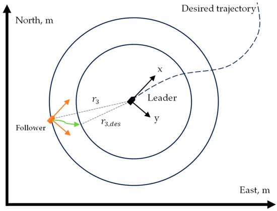
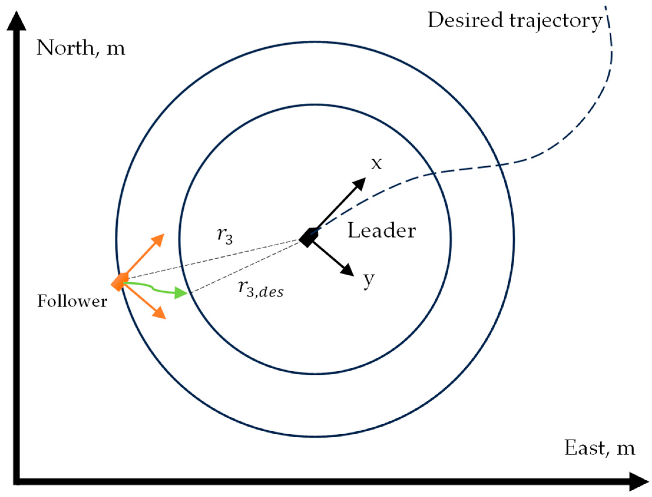
It is assumed that the leader vehicle possesses sufficient onboard computational resources to solve the previously introduced optimal tracking control problem and to generate the corresponding control inputs in real time. The approach described in [27] based on NDOCE FT will be used in this case. In contrast, follower vehicles adopt a lightweight control architecture based on decoupled PID laws. The objective is to maintain a prescribed standoff distance to the leader while aligning depth and attenuating undesired attitudes (Figure 9), thus ensuring a practical trade-off between performance and implementation complexity.

Figure 9. Leader–follower control strategy.

Further, the control law based on NDOCE FT will be considered. For a nonlinear affine system in SDC form

$${\displaystyle \frac{d\mathbb{x}}{dt}}=\mathit{A}\left(\mathbb{x}\right)\mathbb{x}+\mathit{B}\left(\mathbb{x}\right)u, \mathbb{x}\left(t_0\right)={\mathbb{x}}_o$$

(32)

the tracking objective is set for a given signal $\mathbb{r}\left(t\right)$ over a finite interval in accordance with the cost functional

$$\begin{gathered} J\left(u\right)={\displaystyle \frac{1}{2}}{\int }_{t_0}^{t_f}(\left(\mathbb{y}-\mathbb{r}{)}^{T}Q\left(\mathbb{x}\right)\left(\mathbb{y}-\mathbb{r}\right)+u^{T}R\left(\mathbb{x}\right)u\right)dt, \\ Q\left(\mathbb{x}\right)\ge 0,R\left(\mathbb{x}\right)>0, \end{gathered}$$

(33)

where $\mathbb{y}\left(t\right)=\mathit{C}\left(\mathbb{x}\right)\mathbb{x}\left(t\right)$—system’s output defined by (32).

The Hamiltonian for problem (33) is given by

$$H={\displaystyle \frac{1}{2}}\left((\mathbb{y}-\mathbb{r}{)}^{T}Q(\mathbb{x}\left)\right(\mathbb{y}-\mathbb{r})+u^{T}R(\mathbb{x})u\right)+{\lambda }^T\left(\mathit{A}\left(\mathbb{x}\right)\mathbb{x}+\mathit{B}\left(\mathbb{x}\right)u\right).$$

(34)

Optimal control from the necessary optimality condition is written as

$${\displaystyle \frac{\partial H}{\partial u}}=0 \Rightarrow R\left(\mathbb{x}\right)u+{\mathit{B}}^T\left(\mathbb{x}\right)\lambda =0 \Rightarrow u=-R^{-1}\left(\mathbb{x}\right)B^T\left(\mathbb{x}\right)\lambda$$

(35)

For the conjugate variable and the state variable,

$$\begin{gathered} {\displaystyle \frac{d\lambda }{dt}}=-{\displaystyle \frac{\partial H}{\partial \mathbb{x}}}=-{\mathit{A}}^T\left(\mathbb{x}\right)\lambda -{\left[{\displaystyle \frac{\partial \mathit{A}\left(\mathbb{x}\right)}{\partial \mathbb{x}}}\mathbb{x}\right]}^T\lambda -{\left[{\displaystyle \frac{\partial \mathit{B}\left(\mathbb{x}\right)}{\partial \mathbb{x}}}u\right]}^T\lambda -{\displaystyle \frac{1}{2}}{u}^T{\displaystyle \frac{\partial R\left(\mathbb{x}\right)}{\partial \mathbb{x}}}u \\ -{\mathit{C}}^{T}Q\left(\mathbb{x}\right)\mathit{C}\mathbb{x}-{\left({\displaystyle \frac{\partial \mathit{C}\left(\mathbb{x}\right)}{\partial \mathbb{x}}}\mathbb{x}\right)}^{T}Q\left(\mathbb{x}\right)\mathit{C}\mathbb{x}-{\displaystyle \frac{1}{2}}{\left({\displaystyle \frac{\partial Q\left(\mathbb{x}\right)}{\partial \mathbb{x}}}\left(\mathit{C}\mathbb{x}-\mathbb{r}\right)\right)}^T\mathit{C}\mathbb{x} \\ +{\mathit{C}}^{T}Q\left(\mathbb{x}\right)\mathbb{r}+{\left({\displaystyle \frac{\partial \mathit{C}\left(\mathbb{x}\right)}{\partial \mathbb{x}}}\mathbb{x}\right)}^{T}Q\left(\mathbb{x}\right)\mathbb{r}+{\displaystyle \frac{1}{2}}{\left({\displaystyle \frac{\partial Q\left(\mathbb{x}\right)}{\partial \mathbb{x}}}(\mathit{C}\mathbb{x}-\mathbb{r})\right)}^T\mathbb{r} \end{gathered}$$

(36)

Further, using Riccati transformation [36],

$$\mathbb{x}=\mathit{M}\left(\mathbb{x}\right)\lambda +\mathrm{g}\left(\mathbb{x}\right), \lambda ={\mathit{M}}^{-1}\left(\mathbb{x}\right)(\mathbb{x}-\mathrm{g}(\mathbb{x}\left)\right)$$

(37)

Substituting (37) into (35), for control $u$ gives

$$u=-R^{-1}\left(\mathbb{x}\right){\mathit{B}}^T\left(\mathbb{x}\right){\mathit{M}}^{-1}\left(\mathbb{x}\right)(\mathbb{x}-\mathrm{g}(\mathbb{x}\left)\right)=-G\left(\mathbb{x}\right)(\mathbb{x}-\mathrm{g}(\mathbb{x}\left)\right).$$

(38)

Now, differentiate

$$\dot{\mathbb{x}}=\dot{\mathit{M}}\left(\mathbb{x}\right)\lambda +\mathit{M}\left(\mathbb{x}\right)\dot{\lambda }+\dot{\mathrm{g}}\left(\mathbb{x}\right)$$

(39)

and perform a number of transformations using (32), (34) and (35) to obtain (to simplify the notation, the dependence on $\mathbb{x}$ will be omitted in the following cumbersome calculations)

$$\begin{gathered} \left\{\begin{array}{l}\dot{\mathit{M}}-\mathit{M}{\mathit{A}}^T-\mathit{A}\mathit{M}+\mathit{B}{R}^{-1}{\mathit{B}}^T-\mathit{M}{\mathit{C}}^{T}Q\mathit{C}\mathit{M}\\ -\mathit{M}{\left[{\displaystyle \frac{\partial \mathit{A}}{\partial \mathbb{x}}}\mathbb{x}\right]}^T-\mathit{M}{\left[{\displaystyle \frac{\partial \mathit{B}}{\partial \mathbb{x}}}u\right]}^T\\ -\mathit{M}{\left({\displaystyle \frac{\partial \mathit{C}}{\partial \mathbb{x}}}\mathbb{x}\right)}^{T}Q\mathit{C}\mathit{M}-{\displaystyle \frac{1}{2}}\mathit{M}{\left({\displaystyle \frac{\partial Q}{\partial \mathbb{x}}}\left(\mathit{C}\mathbb{x}-\mathbb{r}\right)\right)}^T\mathit{C}\mathit{M}\end{array}\right\}\lambda \\ +\left\{\begin{array}{c}\dot{\mathrm{g}}-\mathit{A}g-\mathit{M}{\mathit{C}}^{T}Q\mathit{C}g+\mathit{M}{\mathit{C}}^{T}Q\mathbb{r}\\ -\mathit{M}{\left({\displaystyle \frac{\partial \mathit{C}}{\partial \mathbb{x}}}\mathbb{x}\right)}^{T}Q\mathit{C}g-\mathit{M}{\left({\displaystyle \frac{\partial \mathit{C}}{\partial \mathbb{x}}}\mathbb{x}\right)}^{T}Q\mathbb{r}-{\displaystyle \frac{1}{2}}\mathit{M}{u}^T{\displaystyle \frac{\partial R}{\partial \mathbb{x}}}u\\ +{\displaystyle \frac{1}{2}}\mathit{M}{\left({\displaystyle \frac{\partial Q}{\partial \mathbb{x}}}(\mathit{C}\mathbb{x}-\mathbb{r})\right)}^T\mathit{C}g+{\displaystyle \frac{1}{2}}\mathit{M}{\left({\displaystyle \frac{\partial Q}{\partial \mathbb{x}}}(\mathit{C}\mathbb{x}-\mathbb{r})\right)}^T\mathbb{r}\end{array}\right\}=0. \end{gathered}$$

(40)

In (38), two parts can be distinguished: the matrix $\mathit{M}\left(\mathbb{x}\right)$ equation

$$\left\{\begin{array}{l}\dot{\mathit{M}}-\mathit{M}{\mathit{A}}^T-\mathit{A}\mathit{M}+\mathit{B}{R}^{-1}{\mathit{B}}^T-\mathit{M}{\mathit{C}}^{T}Q\mathit{C}\mathit{M}\\ -\mathit{M}{\left[{\displaystyle \frac{\partial \mathit{A}}{\partial \mathbb{x}}}\mathbb{x}\right]}^T-\mathit{M}{\left[{\displaystyle \frac{\partial \mathit{B}}{\partial \mathbb{x}}}u\right]}^T\\ -\mathit{M}{\left({\displaystyle \frac{\partial \mathit{C}}{\partial \mathbb{x}}}\mathbb{x}\right)}^{T}Q\mathit{C}\mathit{M}-{\displaystyle \frac{1}{2}}\mathit{M}{\left({\displaystyle \frac{\partial Q}{\partial \mathbb{x}}}(\mathit{C}\mathbb{x}-\mathbb{r})\right)}^T\mathit{C}\mathit{M}\end{array}\right\}=0$$

(41)

and the vector’s $\mathrm{g}\left(\mathbb{x}\right)$ equation

$$\left\{\begin{array}{c}\dot{\mathrm{g}}-\mathit{A}g-\mathit{M}{\mathit{C}}^{T}Q\mathit{C}g+\mathit{M}{\mathit{C}}^{T}Q\mathbb{r}\\ -\mathit{M}{\left({\displaystyle \frac{\partial \mathit{C}}{\partial \mathbb{x}}}\mathbb{x}\right)}^{T}Q\mathit{C}g-\mathit{M}{\left({\displaystyle \frac{\partial \mathit{C}}{\partial \mathbb{x}}}\mathbb{x}\right)}^{T}Q\mathbb{r}-{\displaystyle \frac{1}{2}}\mathit{M}{u}^T{\displaystyle \frac{\partial R}{\partial \mathbb{x}}}u\\ +{\displaystyle \frac{1}{2}}\mathit{M}{\left({\displaystyle \frac{\partial Q}{\partial \mathbb{x}}}(\mathit{C}\mathbb{x}-\mathbb{r})\right)}^T\mathit{C}g+{\displaystyle \frac{1}{2}}\mathit{M}{\left({\displaystyle \frac{\partial Q}{\partial \mathbb{x}}}(\mathit{C}\mathbb{x}-\mathbb{r})\right)}^T\mathbb{r}\end{array}\right\}=0.$$

(42)

At $t=t_0$ (37) gives $\mathbb{x}\left(t_0\right)=\mathit{M}\left(t_0\right)\lambda \left(t_0\right)+\mathrm{g}\left(t_0\right),$ and since $\lambda \left(t_0\right)$ is unknown, it is necessary to assume $\mathit{M}\left(t_0\right)=0$, $\mathrm{g}\left(t_0\right)=\mathbb{x}\left(t_0\right)$ to satisfy the initial conditions. Similarly, at $t=t_f$ (37) gives $\mathbb{x}\left(t_f\right)=\mathit{M}\left(t_f\right)\lambda \left(t_f\right)+\mathrm{g}\left(t_f\right),$ and since $\lambda \left(t_f\right)$ is also unknown, it is necessary to assume $\mathit{M}\left(t_f\right)=0$, $\mathrm{g}\left(t_f\right)=\mathbb{x}\left(t_f\right)$ to satisfy the boundary conditions.

Expressions (38)–(42) are nonlinear differential optimal control equations (NDOCEs). Consider Equations (41) and (42) separately. Neglecting the terms with partial derivatives, the following Riccati differential equation (SDDRE) is obtained:

$$\begin{gathered} \dot{\mathit{M}}=\mathit{M}\left(\mathbb{x}\right){\mathit{A}}^T\left(\mathbb{x}\right)+\mathit{A}\left(\mathbb{x}\right)\mathit{M}\left(\mathbb{x}\right)-\mathit{B}\left(\mathbb{x}\right)R^{-1}\left(\mathbb{x}\right){\mathit{B}}^T\left(\mathbb{x}\right) \\ +\mathit{M}\left(\mathbb{x}\right){\mathit{C}}^T\left(\mathbb{x}\right)Q\left(\mathbb{x}\right)\mathit{C}\left(\mathbb{x}\right)\mathit{M}\left(\mathbb{x}\right). \end{gathered}$$

(43)

and the forward equation for the vector $\mathrm{g}\left(\mathbb{x}\right)$

$$\dot{\mathrm{g}}\left(\mathbb{x}\right)=\left(\mathit{A}\left(\mathbb{x}\right)+\mathit{M}\left(\mathbb{x}\right){\mathit{C}}^T\left(\mathbb{x}\right)Q\left(\mathbb{x}\right)\mathit{C}\left(\mathbb{x}\right)\right)\mathrm{g}\left(\mathbb{x}\right)-\mathit{M}\left(\mathbb{x}\right){\mathit{C}}^T\left(\mathbb{x}\right)Q\left(\mathbb{x}\right)\mathbb{r}.$$

(44)

Practical research into various solutions to nonlinear optimal control problems shows that, although NDOCE provides an optimal solution, the insignificant difference between the NDOCE and SDDRE results allows for the use of expressions (43) and (44), which are simpler to implement.

Unlike the classical optimal trajectory tracking solution, in the proposed solution, the boundary conditions for $\mathit{M}\left(\mathbb{x}\right)$ and $\mathrm{g}\left(\mathbb{x}\right)$ in (43), (44) can be specified both at the initial time $t_0$, and at the final time $t_f$. This allows these equations to be integrated both in the backward direction (as required in the classical solution) and in the forward direction. When moving in the forward direction, there is naturally no problem with insufficient information about the state of the system—a typical problem in SDC optimal control problems that require backward integration.

To avoid the Riccati differential Equation (41), one can require that the following condition be satisfied [27]:

$$\begin{gathered} \dot{\mathit{M}}-\mathit{M}\{{\left[{\displaystyle \frac{\partial \mathit{A}}{\partial \mathbb{x}}}\mathbb{x}\right]}^T-{\left[{\displaystyle \frac{\partial \mathit{B}}{\partial \mathbb{x}}}u\right]}^T-{\left({\displaystyle \frac{\partial \mathit{C}}{\partial \mathbb{x}}}\mathbb{x}\right)}^{T}Q\mathit{C}\mathit{M}-{\displaystyle \frac{1}{2}}{\left({\displaystyle \frac{\partial Q}{\partial \mathbb{x}}}\left(\mathit{C}\mathbb{x}-\mathbb{r}\right)\right)}^T\mathit{C}\mathit{M} \\ -{\left({\displaystyle \frac{\partial \mathit{C}}{\partial \mathbb{x}}}\mathbb{x}\right)}^{T}Q\mathit{C}\mathrm{g}-{\left({\displaystyle \frac{\partial \mathit{C}}{\partial \mathbb{x}}}\mathbb{x}\right)}^{T}Q\mathbb{r}-{\displaystyle \frac{1}{2}}{u}^T{\displaystyle \frac{\partial R}{\partial \mathbb{x}}}u \\ +{\displaystyle \frac{1}{2}}{\left({\displaystyle \frac{\partial Q}{\partial \mathbb{x}}}(\mathit{C}\mathbb{x}-\mathbb{r})\right)}^T\mathit{C}\mathrm{g}+{\displaystyle \frac{1}{2}}{\left({\displaystyle \frac{\partial Q}{\partial \mathbb{x}}}(\mathit{C}\mathbb{x}-\mathbb{r})\right)}^T\mathbb{r}\}=0 \end{gathered}$$

(45)

Equation (45) is called the optimality condition, which in this case is always satisfied under the initial conditions $\mathit{M}\left(t_0\right)=0$. Then, (41) under condition (45) leads to SDRE form

$$\begin{gathered} 0=\bar{\mathit{M}}\left(\mathbb{x}\right){\mathit{A}}^T\left(\mathbb{x}\right)+\mathit{A}\left(\mathbb{x}\right)\bar{\mathit{M}}\left(\mathbb{x}\right)-\mathit{B}\left(\mathbb{x}\right)R^{-1}\left(\mathbb{x}\right){\mathit{B}}^T\left(\mathbb{x}\right) \\ +\bar{\mathit{M}}\left(\mathbb{x}\right){\mathit{C}}^T\left(\mathbb{x}\right)Q\left(\mathbb{x}\right)\mathit{C}\left(\mathbb{x}\right)\bar{\mathit{M}}\left(\mathbb{x}\right) \end{gathered}$$

(46)

and instead of (42) it results in

$$\dot{\bar{\mathrm{g}}}\left(\mathbb{x}\right)=\left(\mathit{A}\left(\mathbb{x}\right)+\bar{\mathit{M}}\left(\mathbb{x}\right){\mathit{C}}^T\left(\mathbb{x}\right)Q\left(\mathbb{x}\right)\mathit{C}\left(\mathbb{x}\right)\right)\bar{\mathrm{g}}\left(\mathbb{x}\right)-\bar{\mathit{M}}\left(\mathbb{x}\right){\mathit{C}}^T\left(\mathbb{x}\right)Q\left(\mathbb{x}\right)\mathbb{r}$$

(47)

The matrix Equation (43) for $\bar{\mathit{M}}\left(\mathbb{x}\right)$ can be solved if the pair of matrices $\left(\mathit{A}\right(\mathbb{x}),\mathit{B}(\mathbb{x}\left)\right)$ is pointwise controllable and the pair $\left(\mathit{A}\right(\mathbb{x}),\mathit{C}(\mathbb{x}\left)\right)$ is observable. In this case, the solution (44) is obtained by integrating from left to right from the initial conditions $\bar{\mathrm{g}}\left(t_0\right)=\mathbb{x}\left(t_0\right)$, and this solution will be bounded [27].

The key advantage of the proposed NDOCE FT optimal tracking control method for nonlinear affine systems over a finite time interval is that it is a one-step procedure due to the use of forward time integration of the corresponding differential equations for the controller components, whose initial conditions are uniquely determined based on the transformation (37) from the initial conditions for the system (32), whereas existing methods based on forward time integration of similar differential equations for the controller components do not provide information about the initial conditions of these equations and require them to be selected in some way. Furthermore, the optimality condition (45) is satisfied precisely by setting special zero initial conditions for matrix $\mathit{M}$, which allows the synthesis of tracking control by limiting differentiation in real time only to Equation (47) for $\bar{\mathrm{g}}\left(\mathbb{x}\right)$, and to determine the $\bar{\mathit{M}}\left(\mathbb{x}\right)$ value by solving the algebraic Equation (46).

The steady-state value of vector $\bar{\mathrm{g}}\left(\mathbb{x}\right)$ can be used in the control calculation, which is determined from (47) when $\dot{\bar{\mathrm{g}}}\left(\mathbb{x}\right)=0$:

$$\bar{\mathrm{g}}\left(\mathbb{x}\right)={\left(\mathit{A}\left(\mathbb{x}\right)+\bar{\mathit{M}}\left(\mathbb{x}\right){\mathit{C}}^T\left(\mathbb{x}\right)Q\left(\mathbb{x}\right)\mathit{C}\left(\mathbb{x}\right)\right)}^{-1}\bar{\mathit{M}}\left(\mathbb{x}\right){\mathit{C}}^T\left(\mathbb{x}\right)Q\left(\mathbb{x}\right),$$

(48)

The leader broadcasts its current position estimation $\left(\widehat{x},\widehat{y},\widehat{z}\right)$. The follower forms the PID input as the error vector using desired distance $r_{3,\mathrm{d}\mathrm{e}\mathrm{s}}$

$$\epsilon =\left[\begin{array}{c}\{\begin{array}{cc}{r}_{3,des}^{\left\{F\right\}}-{\widehat{r}}_3^{\left\{F\right\}}, & \left|\mathrm{atan}2\left({\widehat{y}}^{\left\{L\right\}}-{\widehat{y}}^{\left\{F\right\}}, {\widehat{x}}^{\left\{L\right\}}-{\widehat{x}}^{\left\{F\right\}}\right)-{\widehat{\psi }}^{\left\{F\right\}}\right|<ϵ\\ \hfill 0, & \left|\mathrm{atan}2\left({\widehat{y}}^{\left\{L\right\}}-{\widehat{y}}^{\left\{F\right\}}, {\widehat{x}}^{\left\{L\right\}}-{\widehat{x}}^{\left\{F\right\}}\right)-{\widehat{\psi }}^{\left\{F\right\}}\right|\ge ϵ\end{array}\\ 0\\ {\widehat{z}}^{\left\{L\right\}}-{\widehat{z}}^{\left\{F\right\}}\\ -{\widehat{\phi }}^{\left\{F\right\}}\\ -{\widehat{\theta }}^{\left\{F\right\}}\\ \mathrm{atan}2\left({\widehat{y}}^{\left\{L\right\}}-{\widehat{y}}^{\left\{F\right\}}, {\widehat{x}}^{\left\{L\right\}}-{\widehat{x}}^{\left\{F\right\}}\right)-{\widehat{\psi }}^{\left\{F\right\}}\end{array}\right],$$

(49)

where the label in curly brackets defines the leader’s $\left\{L\right\}$ or follower’s $\left\{F\right\}$ domain.

The second component is set to zero to suppress lateral (sway) motion in steady state. The third component enforces equal depth with the leader. The last component aligns the yaw with the current bearing to the leader, which stabilizes the radial approach/retreat dynamics when regulating $r_3$.

The generalized control input $\tau$ from (27) is computed by channel-wise PID laws:

$$\tau =K_p\epsilon +K_i\int \epsilon dt+K_d\dot{\epsilon }$$

(50)

with diagonal gain matrices and standard anti-windup and rate-limiting provisions.

3. Results

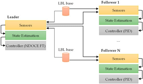
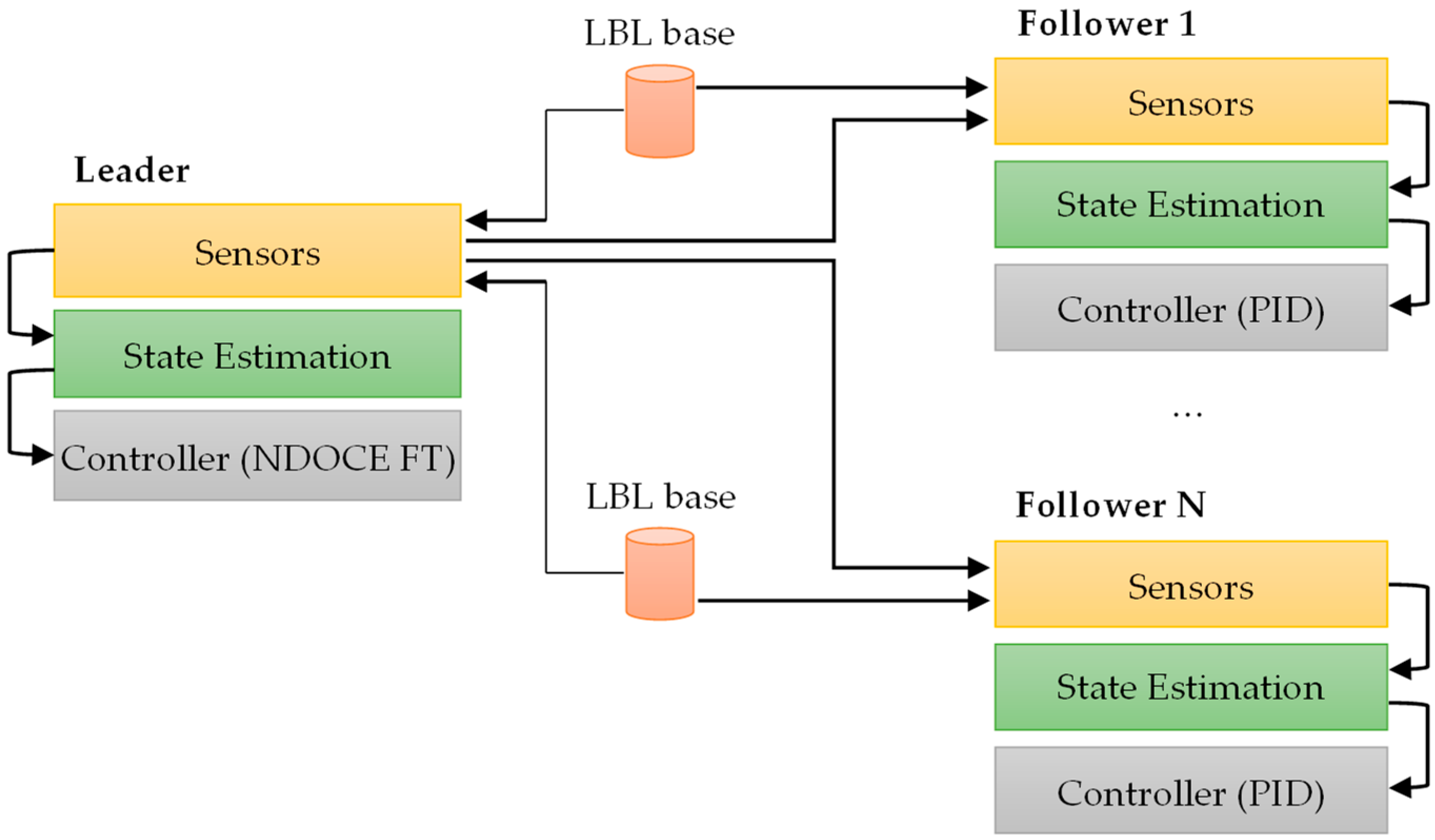
The multi-AUV system is modeled using a leader–follower paradigm (Figure 10). The leader vehicle employs a high-fidelity model for control and estimation, in which the state vector is augmented by slowly varying hydrodynamic parameters. This augmentation improves disturbance rejection and robustness to model–plant mismatch during optimal tracking. The follower vehicles adopt a lightweight control architecture (PID-based) and rely on the leader’s broadcast of reference data and pose estimates. Communication is unidirectional from the leader to the followers; no inter-follower exchange is required.

Figure 10. Leader–follower control system architecture.

The leader’s control input is synthesized by a NDOCE FT controller derived from the nonlinear dynamics and the cost structure in (32)–(48). The plant dynamics and kinematics of each AUV are represented by the continuous-time model in (27). Ranging measurements are generated from geometric relations as in (15). The leader’s estimator operates on the augmented state and implements the Kalman-type recursion specified in (31). Since the NDOCE FT controller acts on the physical (non-augmented) plant state, an extraction step maps the augmented estimate (31) back to the 6-DoF state required by (27), ensuring dimensional consistency between estimation and control.

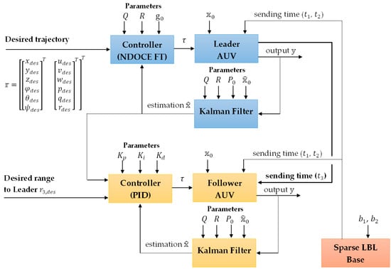
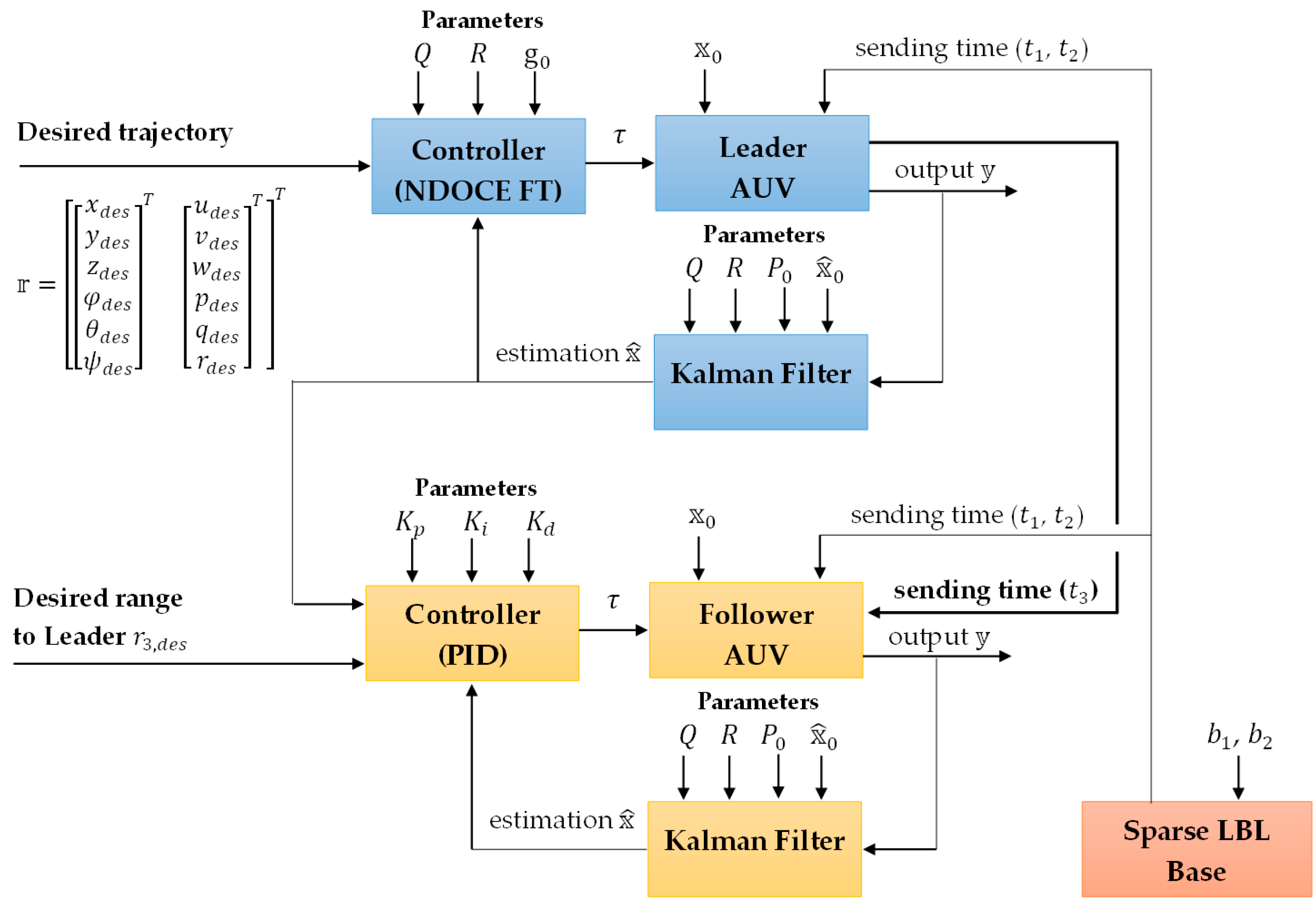
The bidirectional flow between control, plant, and estimation on the leader and follower sides is detailed in Figure 11. On the leader side, “Desired trajectory” supplies the time-parametrized reference used by the optimal tracking design; “Controller (NDOCE FT)” computes the control input according to (32)–(48) using the physical-state estimate provided by selecting the 6-DoF components from the augmented estimate produced by the leader Kalman recursion (31); “Leader AUV” advances the 6-DoF dynamics and kinematics (27) under this input and synthesizes the measurement vector, including range quantities recomputed from instantaneous geometry as in (15); and the leader’s “Kalman Filter” updates the augmented estimate using the applied input (prediction) and measurements (update), closing the leader loop while providing the physical pose for broadcast. On the follower side, “Leader” represents the inbound stream carrying the leader’s estimates; “PID Controller” combines these signals with the follower’s estimated pose and the desired distance to construct the guidance error (including depth matching and yaw alignment to the bearing with standard angle wrapping), which produces the follower input; “Follower AUV” then evolves the 6-DoF model as in (27) and generates local measurements, again recomputed via (15); and “Kalman Filter” realizes the reduced state estimation (11), using the applied input and the measurements to update the physical-state estimate for feedback. Signal conventions (state dimension, ordering, and units) are consistent across blocks; the leader operates with an augmented estimator, whereas the follower loop is entirely physical-state-based. Communication remains unidirectional—from leader to follower—carrying only pose and OWTT, while all measurement synthesis and estimation are executed locally.

Figure 11. Leader–follower control system dataflow diagram.

In the simulations, a configuration with one leader and two followers is assumed. Dynamic parameters for the Fossen 6-DoF formulation, including hydrodynamic contributions, are compiled for the leader and followers in Table 1. The speed of sound in water with a density of $\rho =1000$ is assumed to be $c=1500$. In the simulation model, the external disturbance vector in (24) is assumed zero for the leader and all followers, i.e., ${\bar{f}}_e=0_{6\times 1}$.

The initial conditions used in the simulation are described below. The baseline hydroacoustic transponders are fixed at points $b_1={\left[\begin{array}{ccc}0& -10& 0.5\end{array}\right]}^T$ and $b_2={\left[\begin{array}{ccc}0& 35& 0.5\end{array}\right]}^T$. For the leader, there is an initial state of

$$\begin{array}{c}{\mathbb{x}}_0={\widehat{\mathbb{x}}}_0={\left[\begin{array}{ccccccc}{\eta }_{\mathrm{1,0}}^T& {\eta }_{\mathrm{2,0}}^T& {\nu }_{\mathrm{1,0}}^T& {\nu }_{\mathrm{2,0}}^T& r_{\mathrm{1,0}}& r_{\mathrm{2,0}}& {\mathbb{x}}_{\left\{\mathrm{A}-\mathrm{H}\mathrm{Y}\mathrm{D}\mathrm{R}\mathrm{O}\right\}}^T\end{array}\right]}^T\\ ={\left[\begin{array}{cccc}{0}_{1\times 12}& r_{\mathrm{1,0}}& r_{\mathrm{2,0}}& {\mathbb{x}}_{\left\{\mathrm{A}-\mathrm{H}\mathrm{Y}\mathrm{D}\mathrm{R}\mathrm{O}\right\}}^T\end{array}\right]}^T,\end{array}$$

(51)

where $r_{i,0}={\widehat{r}}_{i,0}=\Vert {\eta }_{\mathrm{1,0}}-b_i\Vert$ at $i=\mathrm{1,2}$. For the leader’s NDOCE FT controller, the initial condition was set as ${\mathrm{g}}_0=\widehat{\mathbb{x}}$.

For the first follower,

$$\begin{array}{c}{\mathbb{x}}_0={\widehat{\mathbb{x}}}_0={\left[\begin{array}{ccccccc}{\eta }_{\mathrm{1,0}}^T& {\eta }_{\mathrm{2,0}}^T& {\nu }_{\mathrm{1,0}}^T& {\nu }_{\mathrm{2,0}}^T& r_{\mathrm{1,0}}& r_{\mathrm{2,0}}& r_{\mathrm{3,0}}\end{array}\right]}^T\\ ={\left[\begin{array}{cccccccc}5& -10& 0_{1\times 3}& \pi /2& 0_{1\times 6}& r_{\mathrm{1,0}}& r_{\mathrm{2,0}}& r_{\mathrm{3,0}}\end{array}\right]}^T.\end{array}$$

(52)

For the second follower,

$$\begin{array}{c}{\mathbb{x}}_0={\widehat{\mathbb{x}}}_0={\left[\begin{array}{ccccccc}{\eta }_{\mathrm{1,0}}^T& {\eta }_{\mathrm{2,0}}^T& {\nu }_{\mathrm{1,0}}^T& {\nu }_{\mathrm{2,0}}^T& r_{\mathrm{1,0}}& r_{\mathrm{2,0}}& r_{\mathrm{3,0}}\end{array}\right]}^T\\ ={\left[-\begin{array}{cccccccc}5& -10& 0_{1\times 3}& \pi /2& 0_{1\times 6}& r_{\mathrm{1,0}}& r_{\mathrm{2,0}}& r_{\mathrm{3,0}}\end{array}\right]}^T.\end{array}$$

(53)

In this case, $r_{i,0}={\widehat{r}}_{i,0}=\Vert {\eta }_{\mathrm{1,0}}-b_i\Vert$ at $i=1, 2$, and the range $r_{\mathrm{3,0}}={\widehat{r}}_{\mathrm{3,0}}$ is equal to the distance between the leader’s ${\eta }_{\mathrm{1,0}}$ and the follower’s ${\eta }_{\mathrm{1,0}}$.

Measurement configuration for the simulation is specified by noise statistics, channel update rates, and estimator–plant timing alignment. Complete numerical values, per-sensor variances and sampling frequencies are reported in Table 2. The initial covariance matrix for the leader and followers $P_0$ was selected as an identity matrix, with the planar position components initialized with inflated uncertainty to reflect the mirror ambiguity transient, i.e., $P_0\left(x,x\right)=P_0\left(y,y\right)=100$.

Table 2. Sensor parameters.

Measurements	Leader	Follower
$r_i$	$1 \mathrm{Hz}|d=10$$, \mathrm{p}\mathrm{p}\mathrm{m}=0.1$	$1 \mathrm{Hz}|d=10$$, \mathrm{p}\mathrm{p}\mathrm{m}=0.1$
$z$	$50 \mathrm{Hz}~\mathcal{N}\left(0, 0.01\right)$	$50 \mathrm{Hz}~\mathcal{N}\left(0, 0.1\right)$
$\varphi$	$25 \mathrm{Hz}~\mathcal{N}\left(0, 0.05\right)$	$25 \mathrm{Hz}~\mathcal{N}\left(0, 0.1\right)$
$\theta$	$25 \mathrm{Hz}~\mathcal{N}\left(0, 0.05\right)$	$25 \mathrm{Hz}~\mathcal{N}\left(0, 0.1\right)$
$\psi$	$25 \mathrm{Hz}~\mathcal{N}\left(0, 0.05\right)$	$25 \mathrm{Hz}~\mathcal{N}\left(0, 0.1\right)$
$u$	$50 \mathrm{Hz}~\mathcal{N}\left(0, 0.025\right)$	$50 \mathrm{Hz}~\mathcal{N}\left(0, 0.05\right)$
$v$	$50 \mathrm{Hz}~\mathcal{N}\left(0, 0.025\right)$	$50 \mathrm{Hz}~\mathcal{N}\left(0, 0.05\right)$
$w$	$50 \mathrm{Hz}~\mathcal{N}\left(0, 0.025\right)$	$50 \mathrm{Hz}~\mathcal{N}\left(0, 0.05\right)$
$p$	$50 \mathrm{Hz}~\mathcal{N}\left(0, 0.05\right)$	$50 \mathrm{Hz}~\mathcal{N}\left(0, 0.075\right)$
$q$	$50 \mathrm{Hz}~\mathcal{N}\left(0, 0.05\right)$	$50 \mathrm{Hz}~\mathcal{N}\left(0, 0.075\right)$
$r$	$50 \mathrm{Hz}~\mathcal{N}\left(0, 0.05\right)$	$50 \mathrm{Hz}~\mathcal{N}\left(0, 0.075\right)$

For state estimation, the process noise covariance diagonal matrix parameters $Q$ and measurement covariance matrices $R$ for the filter components were chosen according to Table 2. The process noise for the augmented components in the state vector is assumed to be Gaussian, centered and with large deviation $~\mathcal{N}\left(0, 10\right)$. For all other components, the process noise is assumed to be negligibly small. For leaders and followers, the $R$ matrix component was set for ranges in accordance with the accepted $~\mathcal{N}\left(0, 0.25\right)$.

The desired leader’s trajectory required by the NDOCE FT controller is shown below as a time-dependent vector function.

$$\mathbb{r}\left(t\right)=\left[\begin{array}{c}15\sin \left(0.5y+0.4\sin \left(y\right)\right)\\ 8\pi t/360\\ 10\\ 0\\ 0\\ \mathrm{atan}2\left(\dot{y},\dot{x}\right)\\ \dot{x}\cos \left(\psi \right)+\dot{y}\sin \left(\psi \right)\\ 0\\ 0\\ 0\\ 0\\ \left(\dot{x}\ddot{y}-\dot{y}\ddot{x}\right)/({\dot{x}}^2+{\dot{y}}^2) \end{array}\right].$$

(54)

The SDRE matrix parameters were set as follows: $Q=1000·{\mathrm{I}}_{12\times 12}$, $R=0.001·{\mathrm{I}}_{6\times 6}$. At the time, the follower PID controller parameters are recorded as follows:

$$\begin{array}{c}{K}_p=\mathrm{diag}\left(\left[\begin{array}{cccccc}10000& 0& 500& 2000& 2000& 50000\end{array}\right]\right),\\ K_i=\mathrm{diag}\left(\left[\begin{array}{cccccc}0& 0& 0& 10& 10& 20\end{array}\right]\right),\\ K_d=\mathrm{diag}\left(\left[\begin{array}{cccccc}1& 0& 10& 5000& 5000& 10000\end{array}\right]\right).\end{array}$$

(55)

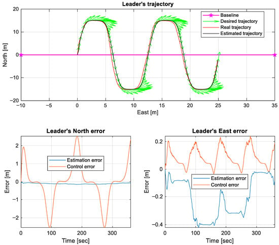
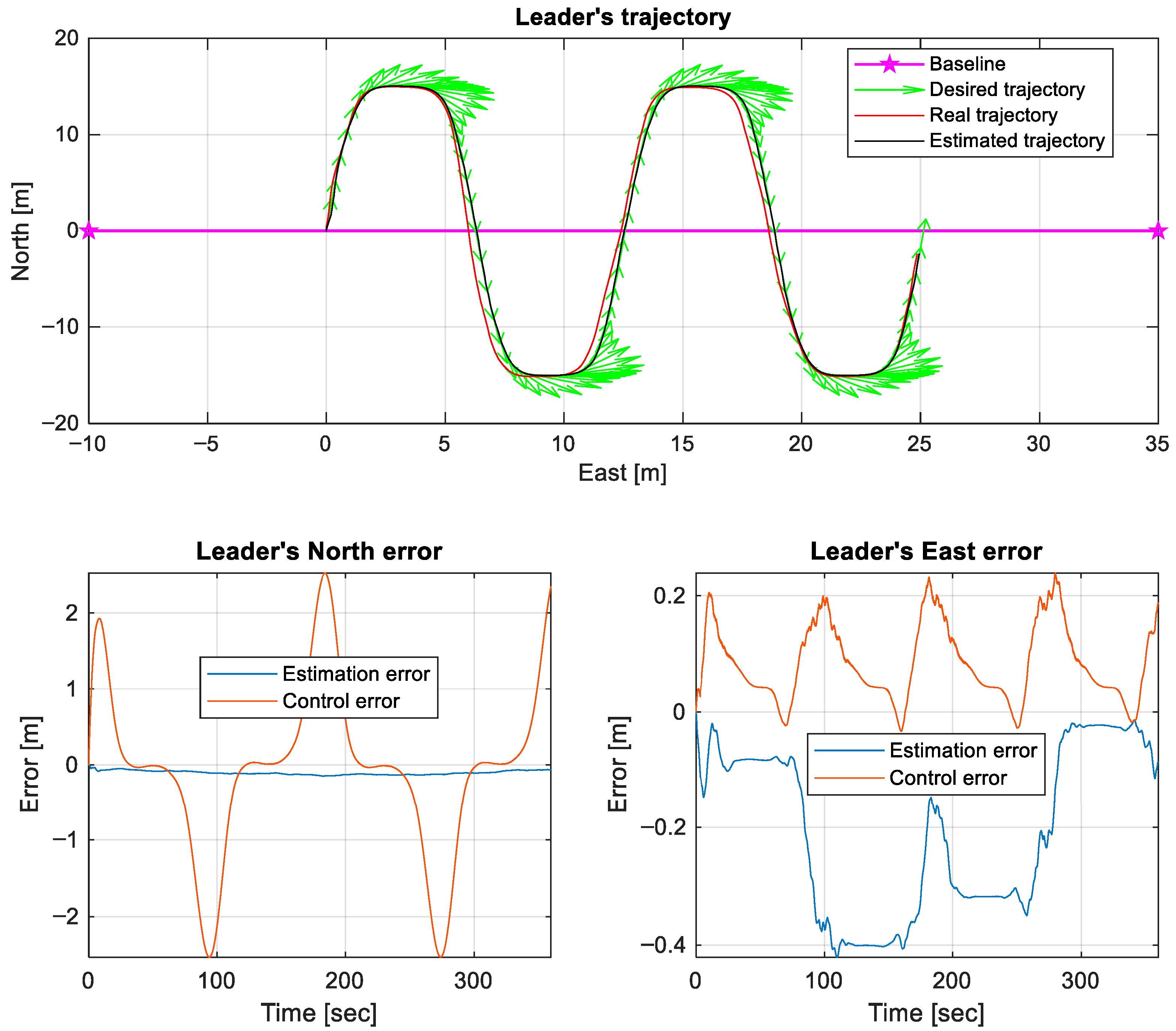
The leader’s desired, ground-truth, and estimated trajectories in planar view and reports estimation and tracking errors along two horizontal axes are presented in Figure 12, where the green arrows show the leader’s course (the third component of (51)) at the specified trajectory key points.

Figure 12. Leader’s trajectory.

The plot is intended to demonstrate rapid convergence by the augmented estimator and small steady-state tracking deviation under NDOCE FT control, with transients confined to the initialization interval. In the presented graph, the estimation error is interpreted as the difference between the true state $\mathbb{x}$ and the estimated state $\widehat{\mathbb{x}}$, and control error is interpreted as the difference between the reference state $\mathbb{r}$ and the estimated state $\widehat{\mathbb{x}}$.

A quantitative assessment of the curves in Figure 12 using the RMSE metric shows that the difference between the estimate and the true coordinates of the leader ($x$, $y$) is (0.105, 0.248) m. The quality of following the specified trajectory relative to the state estimate is determined by the metric as (1.092, 0.107) m, and relative to the true state as (1.092, 0.328) m.

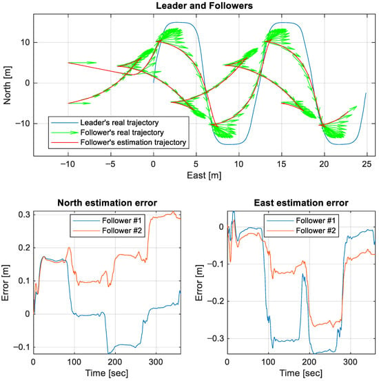
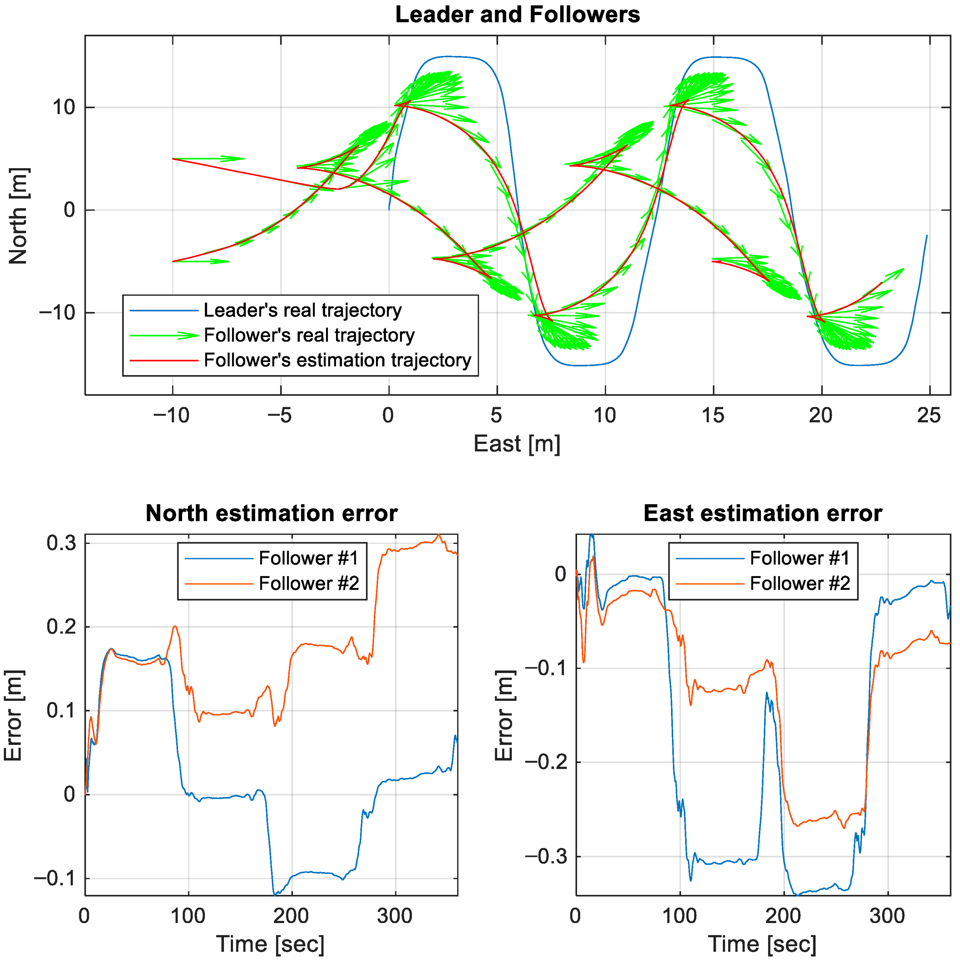
Ground-truth trajectories for the leader and all followers together with their estimates, accompanied by estimation error traces along two axes, are presented in Figure 13, where the green arrows show the followers’ course at key points on the real trajectory. The composite view highlights estimator consistency across vehicles and shows stable follower performance despite absent inter-follower communication. For the first follower, the quality of the ($x$, $y$) coordinate estimation by RMSE is determined as (0.089, 0.216) m, and for the second follower as (0.188, 0.144) m.

Figure 13. Followers’ trajectories.

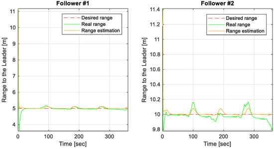
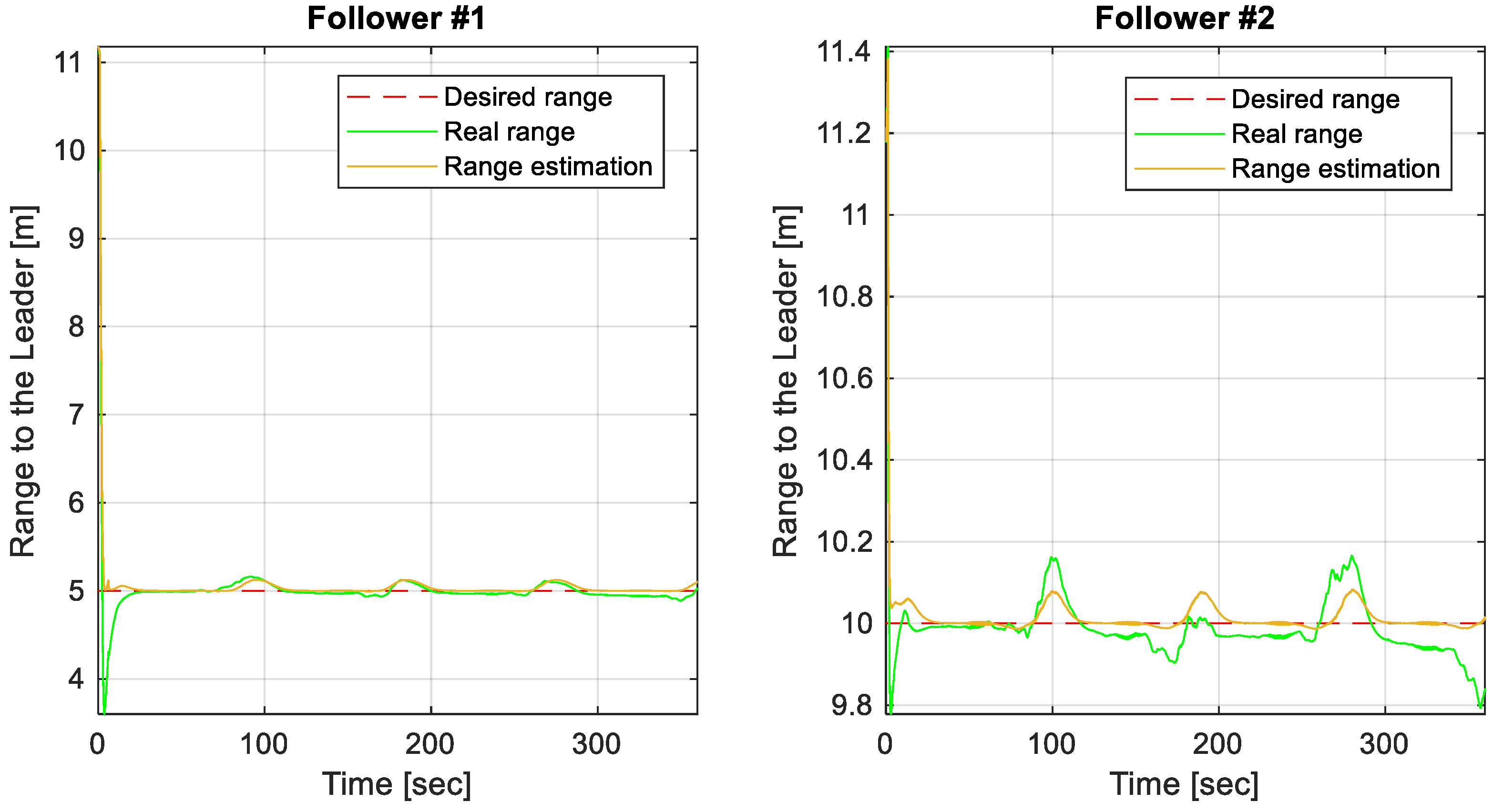
Finally, inter-vehicle ranges between the leader and followers are shown together with their estimates and the reference, followed by range error signals (Figure 14).

Figure 14. Followers’ range error.

The RMSE error in holding the range from the first follower to the leader is 0.5311 m, and the error in holding the true state is 0.536 m. Similarly, the errors for the second follower are 0.1131 m and 0.127 m.

4. Discussion

The presented framework integrates a sparse LBL acoustic infrastructure with asynchronous state estimation and nonlinear tracking control to address the practical constraints in multi-AUV missions. The three-stage schedule with two fixed base transponders establishes a deterministic update period that does not scale with the formation size, thereby reducing channel occupancy while preserving a dedicated downlink for coordination; this communication pattern aligns naturally with leader–follower structures under one-way travel time constraints. The resulting timing regularity improves the estimator–controller interaction and enables consistent formation behavior in simulation. At the same time, it is acknowledged that this schedule is specialized: consensus-type or peer-to-peer topologies require additional uplink/downlink opportunities and cannot be sustained by the fixed three-stage schedule without modification. Thus, the method is strong in directed, broadcast-centric formations but is not intended as a universal networking primitive for all multi-robot architectures.

From the navigation standpoint, the principal challenge in two-base sparse LBL is the binary geometric ambiguity in the horizontal plane. The adopted strategy resolves this ambiguity dynamically by augmenting the state with slant ranges and enforcing temporal consistency through range-rate kinematics; diffuse initialization accelerates convergence in weak geometry, while depth aiding collapses the 3D locus to a tractable planar problem. In contrast to instantaneous trilateration, tight coupling of raw ranges preserves the white noise model and avoids the anisotropic error transformation inherent in pseudo-position updates. Simulation results indicate that, after a short transient, the augmented estimator tracks the correct branch with small innovations even under sparse acoustic updates, which is consistent with the designed predict–update interplay.

The proposed timing subsystem merits separate comment because the OWTT ranging accuracy is limited by timestamp resolution and frequency stability. The microcontroller-based solution with an external high-stability crystal oscillator, coupled directly to a hardware timer via the external trigger input, delivers microsecond-level resolution and sub-ppm stability without resorting to atomic standards. The analysis indicates that such timing performance keeps range errors at the centimeter scale for constant sound speed, which places clock quantization and drift below typical environmental and multipath uncertainties; consequently, oscillator choice at the TCXO/OCXO class is a rational compromise for embedded acoustic ranging units.

On the control side, the leader employs an SDC-based tracking law derived in a NDOCE FT formulation, whereas followers use lightweight PID regulators that maintain standoff distance, align yaw with the instantaneous bearing to the leader, and equalize depth. This asymmetric design leverages the leader’s computational resources and detailed model while keeping follower implementation simple and robust. The reported trajectories show small steady tracking deviations for the leader and stable regulation of leader–follower ranges, which supports the viability of this split architecture in scenarios where unidirectional broadcast is the only reliable link.

A formal stability analysis for the interconnected estimator-controller closed loop lies beyond this study. The intermittent OWTT corrections in the sparse LBL couple tracking performance to estimation transients, which makes rigorous closed-loop guarantees nontrivial. Further analysis of stability and robustness for this interconnection is left for future work.

The limitations are equally notable. The geometry near the baseline, or prolonged motion nearly parallel to it, weakens the cross-track observability and slows disambiguation; occasional maneuvers or deliberate excitation are then beneficial. Depth aiding is assumed; without depth, two slant ranges define a circle in 3D and ambiguity becomes more severe. Environmental variability in sound-speed profiles and multipath can introduce slowly varying biases not fully captured by Gaussian noise models. In the simulation study, the OWTT range model is intentionally simplified by assuming a constant sound speed and independent zero-mean Gaussian range errors, so that the core estimator–controller interaction under sparse updates can be isolated. In operational conditions, sound-speed variability, multipath, and residual timing misalignment may introduce correlated and slowly varying biases that are not fully captured by this noise idealization. Although the third navigation stage can carry integrity and correction data, explicit modeling or online estimation of the sound-speed structure is advisable. The leader is a single point of coordination; while the schedule is resilient to isolated missed receptions, outright leader failure would require a reconfiguration mechanism outside the present scope. Finally, validation was conducted in simulation; sea experiments are needed to quantify sensitivity to currents, scattering, and clock-synchronization drift under operational conditions.

Future work should include field trials with deliberate geometry changes and controlled sound-speed perturbations; integration of Doppler-derived relative velocity from the communication carrier to strengthen along-track corrections; adaptive estimation of environmental parameters within the fusion scheme; and extension of the communication schedule to support redundancy against leader loss while retaining near-deterministic latency. The exploration of smoothing or factor-graph post-processing for map-building and calibration, and systematic tuning of covariance structures to balance responsiveness and noise rejection, are also expected to enhance the robustness.

5. Conclusions

An integrated navigation–control framework was developed for leader–follower AUV formations operating with minimal acoustic infrastructure. The method combines a two-base, three-stage OWTT schedule, a hybrid continuous–discrete estimator with augmented state and diffuse initialization, and an SDRE-based leader controller paired with PID control on the followers. In simulation, the estimator converges rapidly to the dynamically consistent branch, the leader achieves accurate trajectory tracking, and followers maintain prescribed separation with low-bias range estimates under asynchronous updates. The timing subsystem based on a microcontroller and a high-stability crystal oscillator provides microsecond resolution sufficient to bound OWTT range errors at the centimeter scale under constant sound speed, supporting practical embedded implementation.

The architecture is particularly suited to directed formations where deterministic latency, scalability of the update period with respect to group size, and unidirectional broadcast are critical. The strengths include the reduced channel occupancy, elimination of inter-follower links, and robustness to occasional measurement dropouts. The principal constraints arise from the geometry-dependent observability in two-transponder configurations, reliance on depth aiding, and environmental effects not fully captured by idealized noise models. These constraints outline a clear path for future work: sea trials, environmental parameter estimation within the filter, Doppler-aided updates, and schedule extensions for redundancy without forfeiting timing determinism. Collectively, the results indicate that accurate and robust navigation and control are attainable in sparse LBL settings without dense infrastructure, provided that estimation and control are co-designed around the realities of acoustic sensing.

References

- HiPAP. Sparse LBL. Available online: https://www.kongsberg.com/globalassets/kongsberg-discovery/navigation--positioning/apos/hipap-application-note-sparse-lbl.pdf (accessed on 1 September 2025).
- Subsea Positioning Technologies. Available online: https://www.unmannedsystemstechnology.com/wp-content/uploads/2020/06/Subsea-Positioning-Technologies.pdf (accessed on 1 September 2025).
- Fusion 2—Sonardyne. Available online: https://www.sonardyne.com/product/fusion-2/ (accessed on 1 September 2025).
- Çimen, T. Systematic and Effective Design of Nonlinear Feedback Controllers via the State-Dependent Riccati Equation (SDRE) Method. Annu. Rev. Control 2010, 34, 32–51. [Google Scholar] [CrossRef] [Scilit]
- Garin, R.; Bouvet, P.-J.; Tomasi, B.; Forjonel, P.; Vanwynsberghe, C. A Low-Cost Communication-Based Autonomous Underwater Vehicle Positioning System. JMSE 2024, 12, 1964. [Google Scholar] [CrossRef] [Scilit]
- Sonardyne. What is Sparse LBL (range-aiding) used for? Available online: https://www.sonardyne.com/products-knowledge-base/what-is-sparse-lbl-range-aiding-used-for/ (accessed on 10 February 2026).
- Zhang, B.; Ji, D.; Liu, S.; Zhu, X.; Xu, W. Autonomous Underwater Vehicle Navigation: A Review. Ocean Eng. 2023, 273, 113861. [Google Scholar] [CrossRef] [Scilit]
- Masmitja, I.; Gomariz, S.; Del Rio, J.; Kieft, B.; O’Reilly, T. Range-Only Underwater Target Localization: Path Characterization. In Proceedings of the OCEANS 2016 MTS/IEEE Monterey; IEEE: New York, NY, USA, 2016; pp. 1–7. [Google Scholar]
- Vallicrosa, G.; Ridao, P.; Ribas, D.; Palomer, A. Active Range-Only Beacon Localization for AUV Homing. In Proceedings of the 2014 IEEE/RSJ International Conference on Intelligent Robots and Systems; IEEE: New York, NY, USA, 2014; pp. 2286–2291. [Google Scholar]
- Yuan, M.; Li, Y.; Li, Y.; Pang, S.; Zhang, J. A Fast Way of Single-Beacon Localization for AUVs. Appl. Ocean Res. 2022, 119, 103037. [Google Scholar] [CrossRef] [Scilit]
- Diamant, R.; Wolff, L.M.; Lampe, L. Location Tracking of Ocean-Current-Related Underwater Drifting Nodes Using Doppler Shift Measurements. IEEE J. Ocean. Eng. 2015, 40, 887–902. [Google Scholar] [CrossRef] [Scilit]
- Aubry, C.; Forjonel, P.; Bouvet, P.-J.; Pottier, A.; Auffret, Y. On the Use of Doppler-Shift Estimation for Simultaneous Underwater Acoustic Localization and Communication. In Proceedings of the OCEANS 2019—Marseille; IEEE: New York, NY, USA, 2019; pp. 1–5. [Google Scholar]
- Zhang, T.; Chen, L.; Li, Y. AUV Underwater Positioning Algorithm Based on Interactive Assistance of SINS and LBL. Sensors 2015, 16, 42. [Google Scholar] [CrossRef] [Scilit] [PubMed]
- Ribas, D.; Ridao, P.; Mallios, A.; Palomeras, N. Delayed State Information Filter for USBL-Aided AUV Navigation. In Proceedings of the 2012 IEEE International Conference on Robotics and Automation; IEEE: New York, NY, USA, 2012; pp. 4898–4903. [Google Scholar]
- Davari, N.; Gholami, A. An Asynchronous Adaptive Direct Kalman Filter Algorithm to Improve Underwater Navigation System Performance. IEEE Sens. J. 2017, 17, 1061–1068. [Google Scholar] [CrossRef] [Scilit]
- Yang, K.; Zhang, Z.; Cui, R.; Yan, W. Acoustic-Optic Assisted Multisensor Navigation for Autonomous Underwater Vehicles. Ocean Eng. 2024, 297, 117139. [Google Scholar] [CrossRef] [Scilit]
- Fallon, M.F.; Kaess, M.; Johannsson, H.; Leonard, J.J. Efficient AUV Navigation Fusing Acoustic Ranging and Side-Scan Sonar. In Proceedings of the 2011 IEEE International Conference on Robotics and Automation; IEEE: New York, NY, USA, 2011; pp. 2398–2405. [Google Scholar]
- Yan, T.; Xu, Z.; Yang, S.X.; Gadsden, S.A. Formation Control of Multiple Autonomous Underwater Vehicles: A Review. Intell. Robot. 2023, 3, 1–22. [Google Scholar] [CrossRef] [Scilit]
- Li, D.; Du, L. AUV Trajectory Tracking Models and Control Strategies: A Review. JMSE 2021, 9, 1020. [Google Scholar] [CrossRef] [Scilit]
- Geranmehr, B.; Nekoo, S.R. Nonlinear Suboptimal Control of Fully Coupled Non-Affine Six-DOF Autonomous Underwater Vehicle Using the State-Dependent Riccati Equation. Ocean Eng. 2015, 96, 248–257. [Google Scholar] [CrossRef] [Scilit]
- Korayem, M.H.; Nekoo, S.R. Finite-Time State-Dependent Riccati Equation for Time-Varying Nonaffine Systems: Rigid and Flexible Joint Manipulator Control. ISA Trans. 2015, 54, 125–144. [Google Scholar] [CrossRef] [Scilit] [PubMed]
- Heydari, A.; Balakrishnan, S.N. Closed-Form Solution to Finite-Horizon Suboptimal Control of Nonlinear Systems. Int. J. Robust. Nonlinear Control 2015, 25, 2687–2704. [Google Scholar] [CrossRef] [Scilit]
- Korayem, M.H.; Nekoo, S.R. Nonlinear Optimal Control via Finite Time Horizon State-Dependent Riccati Equation. In Proceedings of the 2014 Second RSI/ISM International Conference on Robotics and Mechatronics (ICRoM); IEEE: New York, NY, USA, 2014; pp. 878–883. [Google Scholar]
- Kabanov, A.A. Modified SDRE Method for Finite-Time Nonlinear Optimal Control Problem. In Proceedings of the 2022 International Russian Automation Conference (RusAutoCon); IEEE: New York, NY, USA, 2022; pp. 729–733. [Google Scholar]
- Nekoo, S.R. Tutorial and Review on the State-Dependent Riccati Equation. JAND 2019, 8, 109–166. [Google Scholar] [CrossRef] [Scilit]
- Korayem, M.H.; Nekoo, S.R. State-Dependent Differential Riccati Equation to Track Control of Time-Varying Systems with State and Control Nonlinearities. ISA Trans. 2015, 57, 117–135. [Google Scholar] [CrossRef] [Scilit] [PubMed]
- Kabanov, A.A. Finite-Horizon Optimal Tracking Control for Nonlinear Systems Based on the SDC Method. Mehatronika Avtom. Upr. 2025, 26, 579–587. [Google Scholar] [CrossRef] [Scilit]
- Kramar, V.; Dementiev, K.; Kabanov, A. Optimal State Estimation in Underwater Vehicle Discrete-Continuous Measurements via Augmented Hybrid Kalman Filter. JMSE 2025, 13, 933. [Google Scholar] [CrossRef] [Scilit]
- Kabanov, A.; Kramar, V.; Lipko, I.; Dementiev, K. Cooperative Control of Underwater Vehicle–Manipulator Systems Based on the SDC Method. Sensors 2022, 22, 5038. [Google Scholar] [CrossRef] [Scilit] [PubMed]
- Dhanak, M.R. Springer Handbook of Ocean Engineering; Springer Handbooks Series; Springer International Publishing: Cham, Switzerland, 2016; ISBN 978-3-319-16648-3. [Google Scholar]
- Batista, P.; Silvestre, C.; Oliveira, P. GAS Tightly Coupled LBL/USBL Position and Velocity Filter for Underwater Vehicles. In Proceedings of the 2013 European Control Conference (ECC); IEEE: New York, NY, USA, 2013; pp. 2982–2987. [Google Scholar]
- Skorohod, B.A. Diffuse Initialization of Kalman Filter. J. Automat. Inf. Scien. 2011, 43, 20–34. [Google Scholar] [CrossRef] [Scilit]
- Kabanov, A.A.; Kramar, V.A. The SDC Kalman Filter for Nonlinear System with Uncertainty in Initial Conditions. In Proceedings of the 2020 International Russian Automation Conference (RusAutoCon); IEEE: New York, NY, USA, 2020; pp. 1015–1019. [Google Scholar]
- Fossen, T.I. Handbook of Marine Craft Hydrodynamics and Motion Control, 2nd ed.; Wiley: Hoboken, NJ, USA, 2021; ISBN 978-1-119-57503-0. [Google Scholar]
- Antonelli, G. Underwater Robots; Springer Tracts in Advanced Robotics; Springer International Publishing: Cham, Switzerland, 2018; Volume 123, ISBN 978-3-319-77898-3. [Google Scholar]
- Mufti, I.H.; Chow, C.K.; Stock, F.T. Solution of Ill-Conditioned Linear Two-Point Boundary Value Problems by the Riccati Transformation. SIAM Rev. 1969, 11, 616–619. [Google Scholar] [CrossRef] [Scilit]
Disclaimer/Publisher’s Note: The statements, opinions and data contained in all publications are solely those of the individual author(s) and contributor(s) and not of MDPI and/or the editor(s). MDPI and/or the editor(s) disclaim responsibility for any injury to people or property resulting from any ideas, methods, instructions or products referred to in the content. |
© 2026 by the authors. Licensee MDPI, Basel, Switzerland. This article is an open access article distributed under the terms and conditions of the Creative Commons Attribution (CC BY) license.