


Abstract
One of the major challenges in autonomous path following for unmanned surface vehicles (USVs) is the impact of stochastic environmental forces—primarily wind, waves and currents—which introduce nonlinearities that affect control models. Conventional strategies often rely on minimizing cross-track error, resulting in a reactive system that corrects heading only after a disturbance has displaced the vessel, potentially leading to oscillatory behavior and reduced precision. Deep Reinforcement Learning (DRL) is successfully used for a wide range of nonlinear control tasks. It has already been shown that robust solutions that can handle disturbances such as sensor noise or changes in system dynamics can be obtained. This study investigates whether an agent, provided it can explicitly observe disturbances, can go beyond simply correcting deviations and autonomously learn the correlation between environmental conditions and necessary counter-forces. We show that integrating the wind vector directly into the agent’s observation space allows a Proximal Policy Optimization (PPO) policy to decouple the environmental cause from the kinematic effect, facilitating drift compensation before significant errors accumulate. By systematically comparing agents trained with randomized wind scenarios, we found that agents that can observe the wind can achieve goal reaching rates of up to 99.0% and reduce the spread of path deviation and velocity in our tested scenarios. Furthermore, our results quantify a distinct Pareto frontier between navigational velocity and tracking precision, demonstrating that explicit disturbance perception improves consistency, although robust implicit training already provides substantial resilience. These findings indicate that augmenting state observations with environmental data enhances the stability of learning-based controllers.
1. Introduction
Autonomous path following for unmanned surface vehicles (USVs) is significantly complicated by stochastic environmental forces—primarily wind, waves and currents—which introduce disturbances and nonlinearities that challenge standard control models. These disturbances consist of high-frequency wave oscillations, which are typically filtered to limit actuator wear and low-frequency wind and current forces that induce drift. Conventional strategies often rely on minimizing cross-track error (CTE), resulting in a reactive system that corrects heading after a disturbance has displaced the vessel [1]. In strong environmental conditions, this reactive loop might lead to oscillatory behavior and reduced path following precision [1]. To address this, the study investigates a Deep Reinforcement Learning (DRL) strategy. By integrating the wind vector directly into the agent’s observation space, we enable the policy to decouple the environmental cause from the kinematic effect. Rather than learning solely to correct deviations, the agent is intended to learn to correlate wind conditions with the necessary counter-forces, allowing it to compensate for drift before significant errors accumulate. The main objective is to determine whether an RL agent can use explicit observation of disturbances to autonomously compensate for them.
This publication utilizes an RL framework that was delineated in a previous publication by Krautwig et al. [2]. This framework employs the Robot Operating System (ROS) with the Virtual RobotX (VRX) and enables a systematic variation of environmental parameters and reward functions. This ensures robustness of learned policies to the variability inherent in maritime operations.
Utilizing this framework, the study undertakes a comparative analysis of distinct RL agent configurations. In contrast to research that benchmarks RL against classical methods, our study examines how variations in observation spaces and reward functions influence learning convergence, path following accuracy and generalization. This approach enables the isolation of the impact of specific RL design choices, thereby providing clearer insights into the development of robust autonomous maritime controllers.
1.1. Background
To enable autonomous capabilities in the USV, a Guidance Navigation and Control (GNC) system consisting of guidance, navigation and control modules is typically employed across all USVs [3]. The system is composed of a set of interconnected hardware and software elements that facilitate the execution of navigation and control tasks by the USV. Concurrently, with a ground station—which may be located onshore, on a manned vessel, or a reconnaissance aircraft—navigation data are collected and exchanged between the GNC system and the environment. The system processes these data to modify the vessel’s state, driving it toward the desired goal [1].
GNC systems constitute a mature domain within mobile robotics research [1]. Localization and navigation aim to estimate the robot’s position and motion states with high precision. These tasks are commonly executed using Simultaneous Localization and Mapping (SLAM) algorithms that utilize Extended Kalman Filters (EKFs) to fuse sensor data [4,5]. These methods can generate maps in real time, concurrently with the motion and subsequently update them to categorize map sections according to their occupancy level and thus the hazard they pose to the USV [6,7,8]. Conventional map representations include occupancy grid maps, which encode the occupancy of each map in binary form. As an alternative, extended cost maps are utilized, facilitating the incorporation of supplementary information for each grid cell [5]. This approach enables the delineation of safety boundaries surrounding existing objects, for instance [9].
Approaches to the navigation task are usually based on these map representations and generate a path from the current position to the desired destination. The objective of determining such a path is to identify a collision-free route that is as short as possible, while considering secondary conditions such as waterway limitations or intermediate destinations [10].
The implementation of global path planning frequently involves heuristic graph-based methods, which are capable of calculating a collision-free path on a grid map [1,11]. Examples of such algorithms include the Dijkstra algorithm-based A* and Theta* algorithms [11,12]. These heuristic methods incur high computational costs when applied to large maps and lack the capability to incorporate constraints such as energy optimality [11,12]. Probabilistic path planning methods, such as Rapidly Exploring Random Trees (RRTs) and their variants, offer distinct advantages. Notably, algorithms like RRT* enable asymptotic optimality regarding the shortest path [13]. In general, static objects are the only type of objects that can be included in path planning, unless the path is subject to regular updates [11,12,14].
Guidance and navigation methods are introduced briefly in the following. Model Predictive Controllers (MPCs) are commonly used optimization-based navigation methods. They enable integrated guidance of the USVs with simultaneous control [15,16]. By taking future states into account, reliable control performance of the dynamic system can be achieved, especially if disturbances are estimated [15,16]. In addition, the cost function can be individually designed, whereby the deviation from a global path, and the proximity to an obstacle and the actuator power are typical cost function terms. A notable disadvantage associated with MPCs is their dependence on sufficiently accurate prediction models, which necessitate substantial computational resources [17]. Furthermore, time and effort must also be invested in parameterizing the model and calibrating the cost function weights. This motivates the development of a self-learning controller that takes over the task of guidance including dealing with disturbances [15,16,18,19,20].
In addition to the combined guidance and control solutions, such as the MPC, dedicated controllers also exist. Line-of-sight (LOS) systems using PID controllers can accurately follow planned trajectories [21,22]. Adaptive and learning-based methods, such as Reinforcement Learning (RL) or Imitation Learning, enable flexibility in dynamic environments, though often at the cost of poor interpretability or high training effort [23]. In over-actuated systems, thrust allocation can be used to convert USV motion requests into actuator commands, enabling the integration of additional optimization criteria such as actuator energy efficiency [24].
1.2. Related Works
Recent literature in autonomous maritime control demonstrates a trend toward the integration of DRL for handling nonlinear environmental disturbances, transitioning from simple path planning to complex dynamic trajectory tracking. These studies are broadly distinguished by their choice of action spaces and their strategies for disturbance rejection, ranging from implicit robust training to explicit state-augmented compensation. RL-based strategies address trajectory planning and reference tracking, often combining navigation and control functions. Unlike MPCs, DRL operates without explicit models, allowing agents to derive optimal policies directly from interaction with the environment [4,25]. The RL approach can learn to handle complex environments, demonstrating robust adaptability and the capacity to generalize from environment data [23].
An important distinguishing feature of different explorations in the literature is the variety of scenarios. Often only a few scenarios are used for training and testing, whereby no scenario variations are performed, which may question the generalizability of the results. This section presents a selection of publications with regard to their application, RL approach and considered scenarios [26].
For global path planning, Li et al. [27] propose a Deep Q-Network-based (DQN) approach augmented with Artificial Potential Fields (APFs) to guide unmanned surface vehicles (USVs) through static environments. Their method demonstrates adaptability to varying obstacle configurations and achieves efficient convergence in training. The integration of APF enhances the agent’s ability to avoid local minima, resulting in smoother trajectories and reduced path length compared to baseline DQN implementations. Zhao et al. [28] employ a Deep Deterministic Policy Gradient-based (DDPG) framework for navigation in randomized static environments. The study utilizes a 320 × 320 grid-based map with fixed wind and current parameters and randomly designed rectangular obstacles. Their results indicate that the continuous action space of DDPG enables finer control over heading adjustments, leading to more stable path execution and lower cumulative reward variance across episodes.
Zhong et al. [29] employ a DDPG-based path following controller, which is validated both in simulation and on a full-scale USV. The training phase utilizes randomly generated start and target points within a by area, while the evaluation phase employs specific verification tracks, eight-shaped path simulations with induced action execution delays and real-world field tests on a lake following a triangular route. The method achieves a low CTE and reduced rudder activity, thereby indicating reliable trajectory tracking at minimal control effort. Deraj et al. [30] utilize a DQN-based strategy for reference tracking. The training phase utilizes randomly generated destination waypoints within a specified radial distance in calm water simulations, while validation involves tracking circular, elliptical and figure-eight paths under simulated calm and windy conditions. Although the discrete action space introduces minor chattering due to limited control granularity, the proposed approach achieves path following accuracy comparable to traditional PD controllers and demonstrates robustness in structured environments.
Qu et al. [31] propose a hierarchical path following control scheme for under-actuated Autonomous Marine Vehicles (AMVs) facing model uncertainties and environmental disturbances. The method integrates a surge-heading joint guidance law at the kinematic level with a DRL controller at the dynamic level. Specifically, the authors enhance the Twin-Delayed Deep Deterministic Policy Gradient (TD3) algorithm by incorporating Long Short-Term Memory (LSTM) networks to better handle historical state data and non-Markovian dynamics. A hybrid reward function is utilized to balance tracking accuracy with control stability, effectively penalizing aggressive actuator oscillation. Simulation results demonstrate that this LSTM-TD3 approach achieves faster convergence and lower steady-state errors compared to traditional DDPG and A3C baselines.
Dong et al. [32] introduce a model-based RL control method using PPO to address path-following tasks for ships under environmental disturbances like wind, waves and currents. The approach incorporates a disturbance model to simulate maritime conditions and utilizes PPO to learn optimal control strategies by interacting with this environment. The experimental setup involves training the agent over 1000 episodes using a stochastic environmental disturbance model and subsequently testing path following performance on a parametric circular trajectory and a simulation within the Wuhan section of the Yangtze River. Simulation results using the CyberShip II model demonstrate the method’s ability to achieve high tracking accuracy (final position error < ) and robustness against random perturbations. This study highlights the potential of integrating system dynamics models with RL to enhance the adaptability and reliability of autonomous ship navigation in complex sea environments.
1.3. Contribution
Our study addresses the need for robust and statistically tested control strategies in autonomous maritime navigation. Although the existing literature often reports exemplary results from limited test cases, this work introduces an evaluation framework for DRL agents applied to path-following tasks. The primary contributions are summarized as follows:
- Systematic evaluation of disturbance perception: We conduct a comparative analysis between path following agents operating with implicit environmental awareness and those utilizing explicit wind vector observations. This investigation quantifies the specific performance gains—in terms of stability and precision—achieved by augmenting the observation space with disturbance data.
- Pareto analysis of reward functions: By systematically varying reward weights, we identify and visualize the trade-off (Pareto frontier) between navigational velocity and CTE. This provides insights into the sensitivity of the policy to reward shaping.
- Statistical robustness assessment: To ensure generalization across diverse operational conditions, we employ a domain randomization approach involving stochastic wind vectors and variable path geometries. Performance is assessed using comprehensive statistical metrics—including box plots and scatter plots—over test sets.
This paper is organized as follows: Section 2 details the simulation framework architecture, the formulation of the RL problem and the methodology for scenario generation. Section 3 presents the simulative experiment results, discussing the behavioral differences between agent configurations and the impact of environmental disturbances on learning convergence. Finally, Section 4 summarizes the findings and outlines the implications for the development of robust autonomous maritime controllers.
2. Methodology
This section presents the simulation framework used to investigate RL-based control strategies for USVs. Section 2.1 introduces the architecture of the training framework, including the simulation environment, agent-environment interaction and the thrust allocation. Section 2.2 defines the RL problem for path-following tasks, detailing the respective observation and action spaces, reward functions and scenario generation procedures. The framework used is based on that introduced in Krautwig et al. [2]. However, for the path-following use-case, not only the scenario generation but also the formulation of the RL problem was adapted.
2.1. Framework Architecture
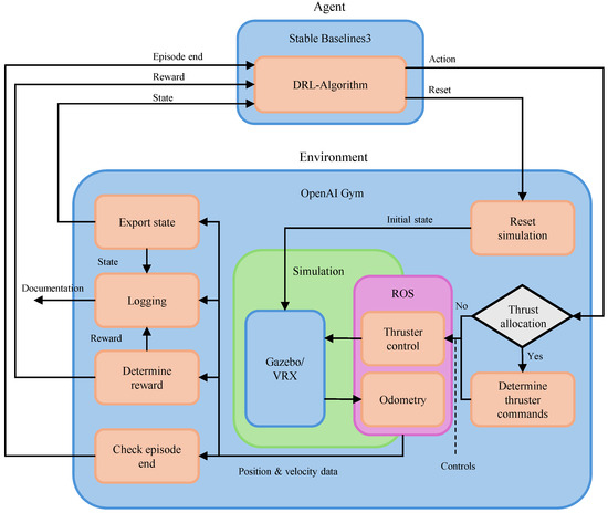
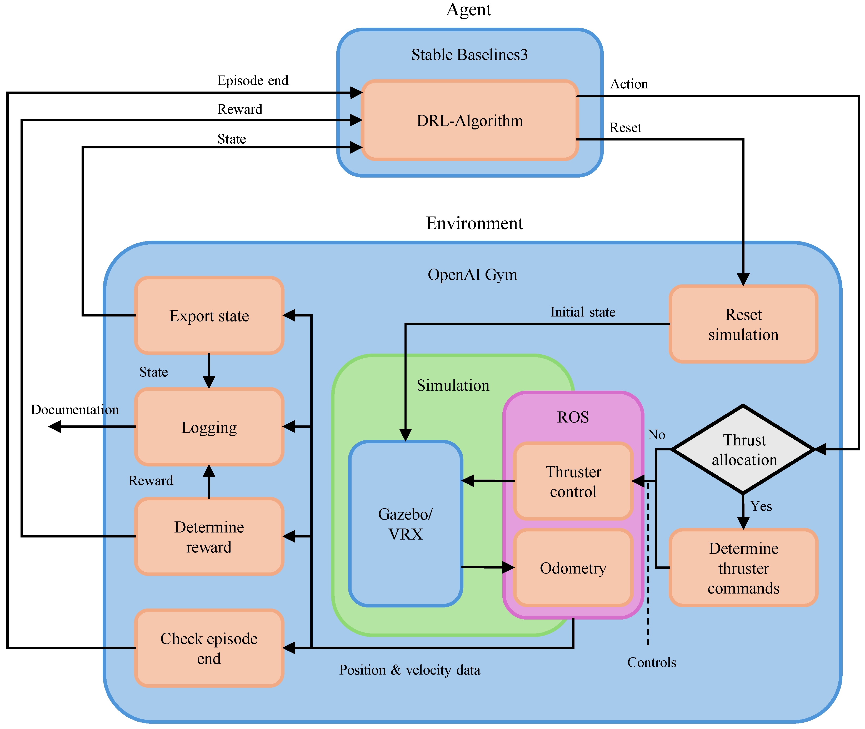
Figure 1 illustrates the RL training architecture, detailing the signal flows and interaction between the agent and the simulation environment. The agent utilizes the DRL algorithms from Stable Baselines3 [33], while the environment adheres to the OpenAI Gym interface [34]. At the core of the environment, the simulation is realized in Virtual RobotX (VRX) [35], which simulates the behavior of USV operating in water environments. VRX allows the integration of ship models, such as the Wave Adaptive Modular Vehicle (WAMV) and other static or dynamic objects, into the simulation environment. Communication between the RL agent and the simulation environment is handled via Robot Operating System (ROS) [36]. Through this interface, control commands are sent to the WAMV’s actuators and odometry data are retrieved. These data are used to evaluate the current state, reward and episode termination condition.
Figure 1.
Architecture of the RL framework [2].
The agent interacts with the environment using the reset and step methods of OpenAI Gym [34]. In the beginning of each episode, the simulation and environment scenario are reset to their initial states. If thrust allocation is enabled, the selected action is first translated into actuator-level control commands, ensuring that the propulsion system is actuated according to its physical constraints and maneuvering capabilities. The simulation environment allows for idealized motor control, whereas a real motor is limited in terms of speed gradients. The thrust allocation has to be calibrated accordingly before it can be applied to real systems. The final reward and state are then returned to the agent. If thrust allocation is disabled, the agent could control the thrusters directly. Thrust allocation is used to exploit actuator redundancy in over-actuated marine vessels and enables the system to distribute control commands optimally among multiple thrusters. Further details on the framework, thrust allocation and their implementation can be found in the publication on the framework from Krautwig et al. [2].
2.2. Scenario Overview and Definition of the Reinforcement Learning Problems
This study investigates the application of RL methods to maritime path following (PF). The inclusion of dynamic obstacles in the RL formulation and the resulting evasive trajectories are not examined in this study from Krautwig et al. [2]. Safe maneuvering with these obstacles is explored in the previous publication. The agent is designed to follow a pre-calculated path with maximum velocity and minimum path deviation. This study focuses on an intrinsic comparative analysis of RL agent configurations to isolate the effects of reward shaping and observation spaces, rather than benchmarking against external control baselines. The main research question is whether the agent can compensate for disturbances on its own by observing disturbance variables. To answer this question, two different scenarios (PF1 and PF2) are introduced, which differ in terms of the observation space.
- PF1—Path following without disturbance observation:The objective in this scenario is for the USV to accurately track a predefined reference trajectory without the observation of disturbances. Here, the agent can observe its own motion states as well as its position and orientation relative to relevant path points. Further details are described in the following subsections.
- PF2—Path following with disturbance observation:In addition to the observation variables introduced in PF1, information about wind speed and direction is provided to the agent during training and testing.
2.2.1. Action Space
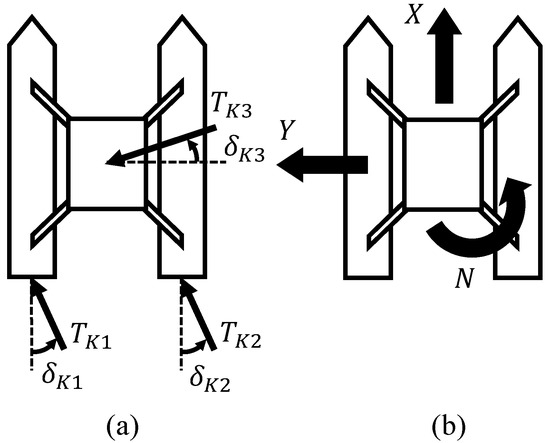
The RL agent’s action space in both path-following scenarios is defined via a thrust allocation vector to ensure generalizability across motor configurations:
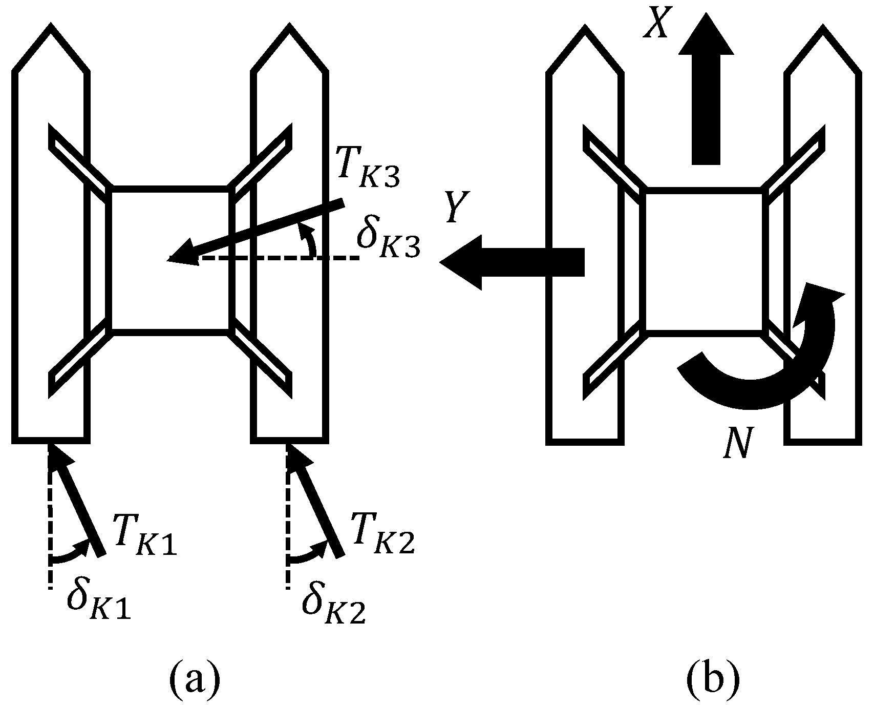
where X and Y are the surge and sway forces and N is the yaw moment in the body-fixed frame (see Figure 2).
Figure 2.
Visualization of thrust allocation (WAMV T1-Configuration): (a) individual thrusters , and with their respective orientation angles , and ; (b) the resulting force components in the global X and Y directions and the rotational moment N around the vehicle’s center.
2.2.2. Observation Space
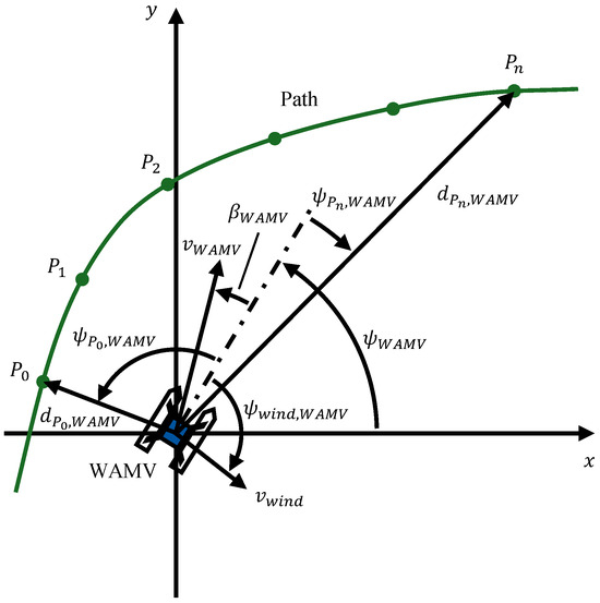
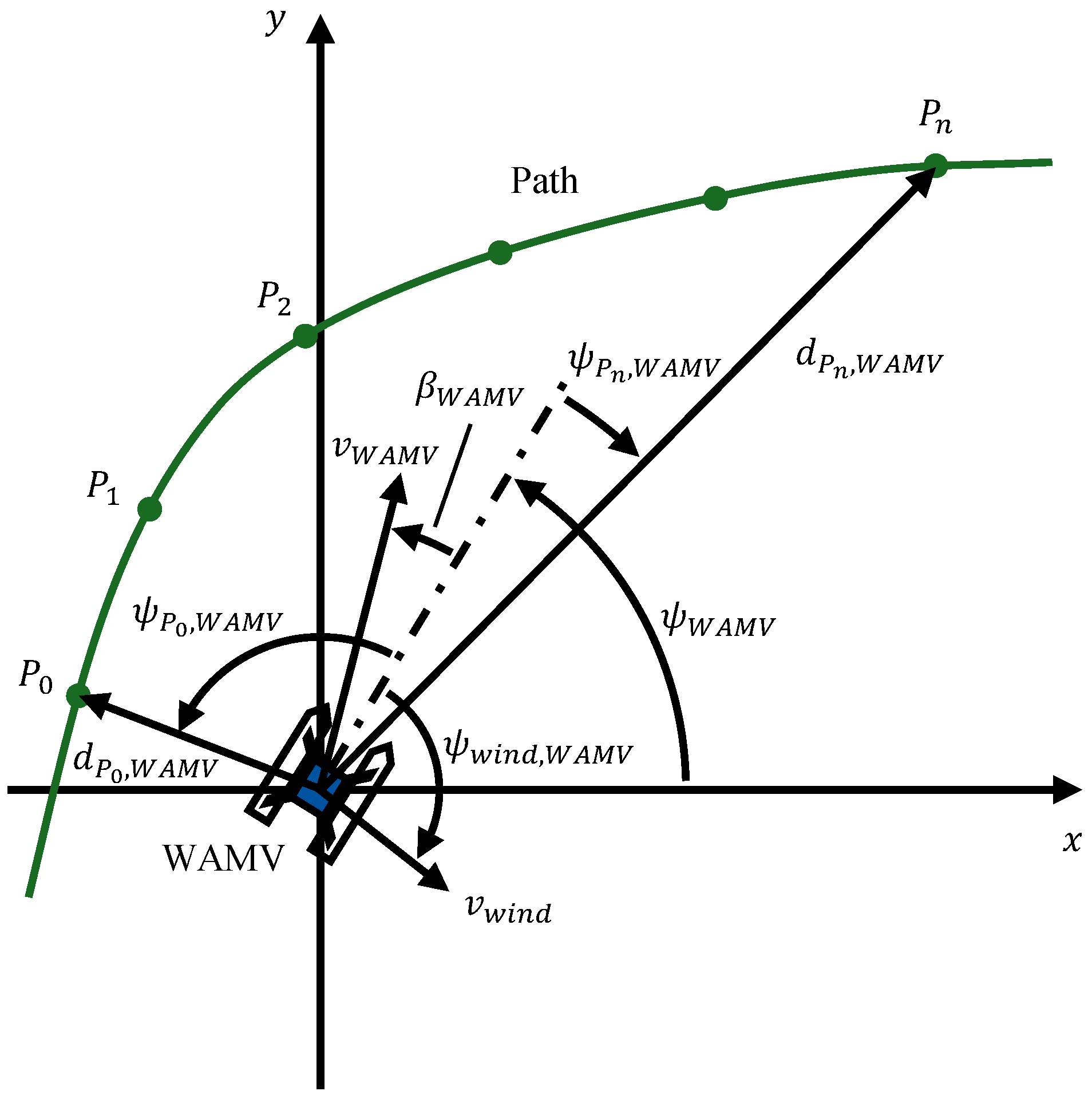
In the PF1 scenario, the observation vector provides the agent with crucial information regarding its own dynamic state and its spatial relationship to the predefined path. The vector is composed of seven distinct components, which are visualized in Figure 3, and it is described in Equation (2):
Figure 3.
Geometric visualization of the components of the observation vectors and .
The path is generated by a global path planner using the Theta* algorithm, with an implementation based on [37]. It will be described further in Section 2.2.4. The first four components of the observation vector describe the vessel’s position relative to this path. Specifically, represents the Euclidean distance to the nearest waypoint, while is the relative angle between the vessel’s heading and the direction to that waypoint. To enable anticipatory maneuvers, and denote the distance and relative angle to a look-ahead waypoint situated n steps further along the path. The remaining three variables characterize the vessel’s motion: is the magnitude of the velocity, is the drift angle (representing the difference between the vessel’s heading and its actual velocity vector), and is the yaw rate, which describes the vessel’s rotational velocity about its vertical axis.
The relative distance between the WAMV’s position and a waypoint of the path is determined as
In order to observe the orientation to the path, the relative angle of the WAMV to a waypoint is calculated, where is the yaw angle of the WAMV:
The observation vector in the PF2 scenario is extended to include global wind speed and relative wind direction to the WAMV :
Thereby, the relative wind direction is calculated as
with describing the global wind direction.
2.2.3. Reward Function
The total reward is composed of a step-wise reward and an episode reward :
The CTE is calculated to penalize the distance to the path. It is defined as the perpendicular distance from the current position of the WAMV to the line segment between two consecutive path waypoints and selected based on the minimum path distance:
Subsequently, the reward for each step is calculated, consisting of the following three reward terms: , , and . The parameters are tunable parameters for each reward term. The reward function is designed using classical reward function definitions, which are described in Abouelazm et al. [38]:
- Cross-track error (CTE) penalty to penalize the distance from the path:
- Reward for velocity towards the path goal (VTPG) with the actual boat velocity and the distance vector to the look-ahead waypoint. This reward is intended to encourage the agent to travel target-oriented:
- A constant time penalty per step to penalize slow traveling:
The full step reward is then calculated by
The episode reward rewards reaching the target position and penalizes timeouts. Timeouts are triggered when a predefined step limit is reached (see Section 2.2.4). The episode reward is defined as
2.2.4. Scenario Generation
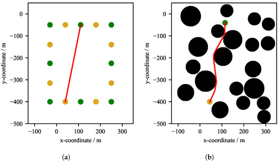
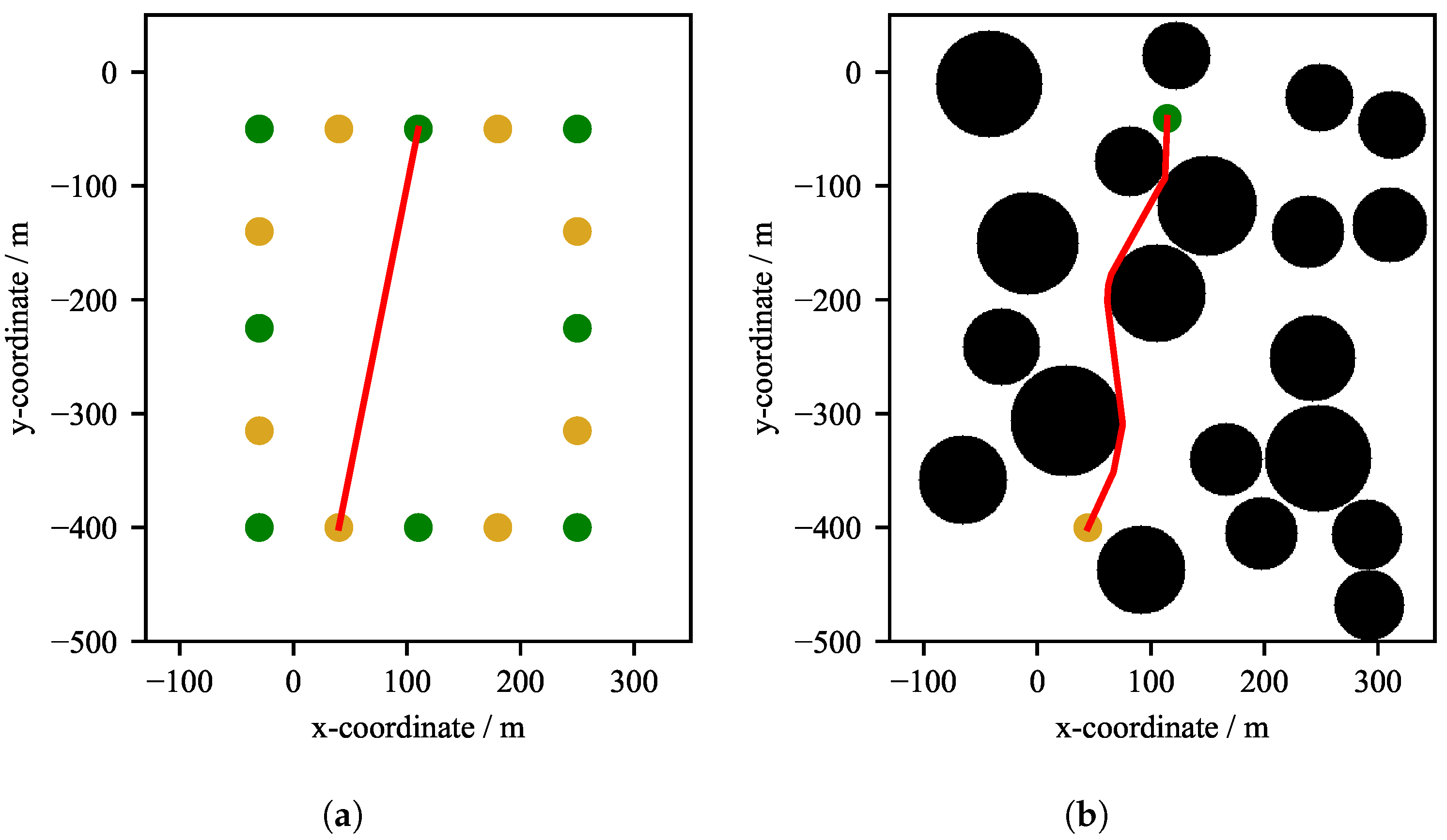
The paths for both scenarios are created and randomly generated by adding virtual obstacles to the global planner’s map to force the generation of nonlinear paths. The RL agent does not observe these obstacles directly; its objective is strictly to follow the resulting path. These virtual obstacles are circular in varying size and position (see Figure 4b). Start and target points of a path are varied to create a randomized path—possible positions are shown in Figure 4a. The workspace is represented by the size of the map depicted. If the agent exits in this space, the episode is terminated as unsuccessful. The path planning is carried out using a Theta* algorithm, whereby the algorithm of the navigation stack Nav2 is used [9].
Figure 4.
Visualization of a PF scenario: (a) Positions of all possible start points (green) and target points (yellow). (b) Theta* path through virtual random obstacles from the start to the target position.
During training, at least 1600 episodes are executed for PF1 and PF2, respectively. To facilitate initial learning, agents are always trained without disturbances for the first 100 episodes, even if a scenario with disturbances is being trained. This approach allows the agent to focus exclusively on path-following behavior in the early stages. This form of curriculum learning has demonstrated improved learning performance and convergence during development and is derived from similar learning tasks in robotics, similar to the approach in Florensa et al. [39]. The minimum number of episodes results from a total training budget of 400,000 steps, which corresponds to 1600 episodes with a maximum of 250 steps each. In practice, episodes often terminate before reaching the step limit so that additional episodes are appended with the remaining steps.
When disturbances are enabled, the simulation uses the wind models provided by VRX [35]. Although operational USVs encounter a superposition of wind, waves and currents, this study deliberately restricts the simulation scope to wind disturbances. Since inland lakes are considered, currents are neglected in this publication. Due to the design of the WAMV, waves affect its movements differently than they affect a mainly rigid ship that is mostly dimensionally stable. Therefore, waves are omitted due to the technical difficulty of extracting them as reliable observation variables within the VRX framework. Utilizing the VRX physics engine, the wind is modeled via a Harris spectrum to introduce stochastic nonlinearities. In scenario generation, the mean wind speed and standard deviation are each varied in steps within the range of 0 m/s to 10 m/s. These parameters allow us to simulate severe environmental conditions, corresponding to a force of up to 8 on the Beaufort scale. The global direction of the wind is varied from 0° to 330° in increments of 30°. This results in 1441 possible discrete wind variations: 11 mean wind variations × 11 wind standard deviation variations × 12 wind directions and 11 zero wind scenarios. To enable a statistical evaluation of agents, all agent variations are subjected to the same scenario variations. This means that the randomly selected wind speeds and directions, as well as the randomly generated paths, are applied equally to all agents during training and testing using the same seed.
While recent RL applications demonstrate adaptability, validation is frequently restricted to a narrow set of fixed scenarios, lacking the statistical robustness ensured by automated, broad-scale scenario generation. Furthermore, standard strategies often address environmental forces purely reactively, leaving the potential for agents to explicitly observe and learn the correlation between stochastic wind vectors and drift compensation largely unexplored. These methodological gaps motivate the presented work, which utilizes a framework designed for systematic scenario randomization to evaluate the impact of disturbance observation on navigational stability.
3. Results and Discussion
This section presents the training results of the various scenarios. For testing, the agents are executed in the same scenario in which they were trained over 200 episodes. The step limit per episode is identical to the training (250 steps). However, a different variation of the scenarios is used in the testing phase; for example, paths or disturbance variables such as wind are modified. To ensure comparability of the evaluation results across all scenarios and agents, the same set of 200 test scenario variations is used for all agents of one scenario. To analyze the impact of reward shaping on the agent’s behavior, multiple variations of the reward weights (velocity towards path goal) and (cross-track error) are considered; while these parameters are varied, the remaining parameters are held constant throughout all experiments: , , and . In a multi-term reward function, the agent’s emergent policy is governed by the relative dependencies and ratios between the competing reward components, not their absolute magnitudes. Due to the computational effort and the focus on trade-off considerations in this study, a comprehensive factorial analysis of all parameters is not conducted and the parameter study is limited to nine representative weight combinations.
The variation name encoding of the parameter combinations is summarized in Table 1. This setup enables a focused investigation of the trade-offs between path following, goal reaching behaviors and disturbance resilience. An example is the agent configuration (C) C1_1_1. This agent is trained in scenario (S) PF1, and the parameters are (X) and (Y).
Table 1.
Agent’s configuration encoding for variations of and and disturbance variations used in the reward function.
3.1. Scenario PF1—Path Following Without Disturbance Observation
This subsection presents a detailed evaluation of the agent’s performance in path following without disturbance observations (PF1). First, the general path-following behavior is examined by analyzing representative trajectory plots, which are utilized to qualitatively assess the maneuvering behavior of trained agents. Subsequently, a quantitative investigation is conducted to explore the trade-off between theoretical mean velocity and mean CTE, which reflects the balance between navigational efficiency and path-following accuracy. Importantly, the objective of this study is not merely to present the performance of a single optimized agent, but rather to systematically investigate and communicate the influence of different algorithmic and environmental parameters on agent behavior. This approach aims to enhance the interpretability of RL outcomes and shall support the decision-making in the design of autonomous maritime control systems.
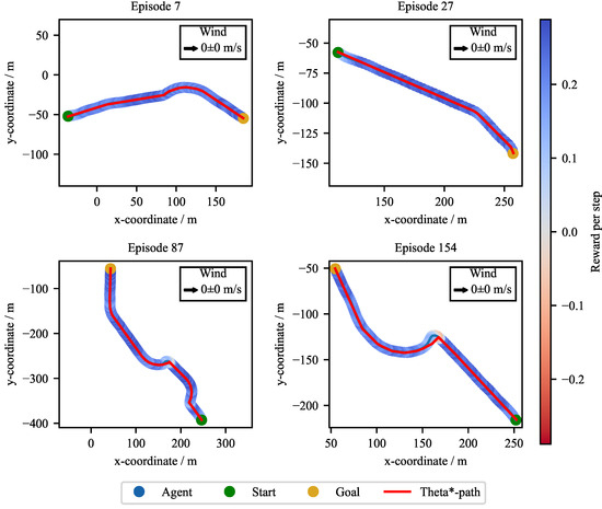
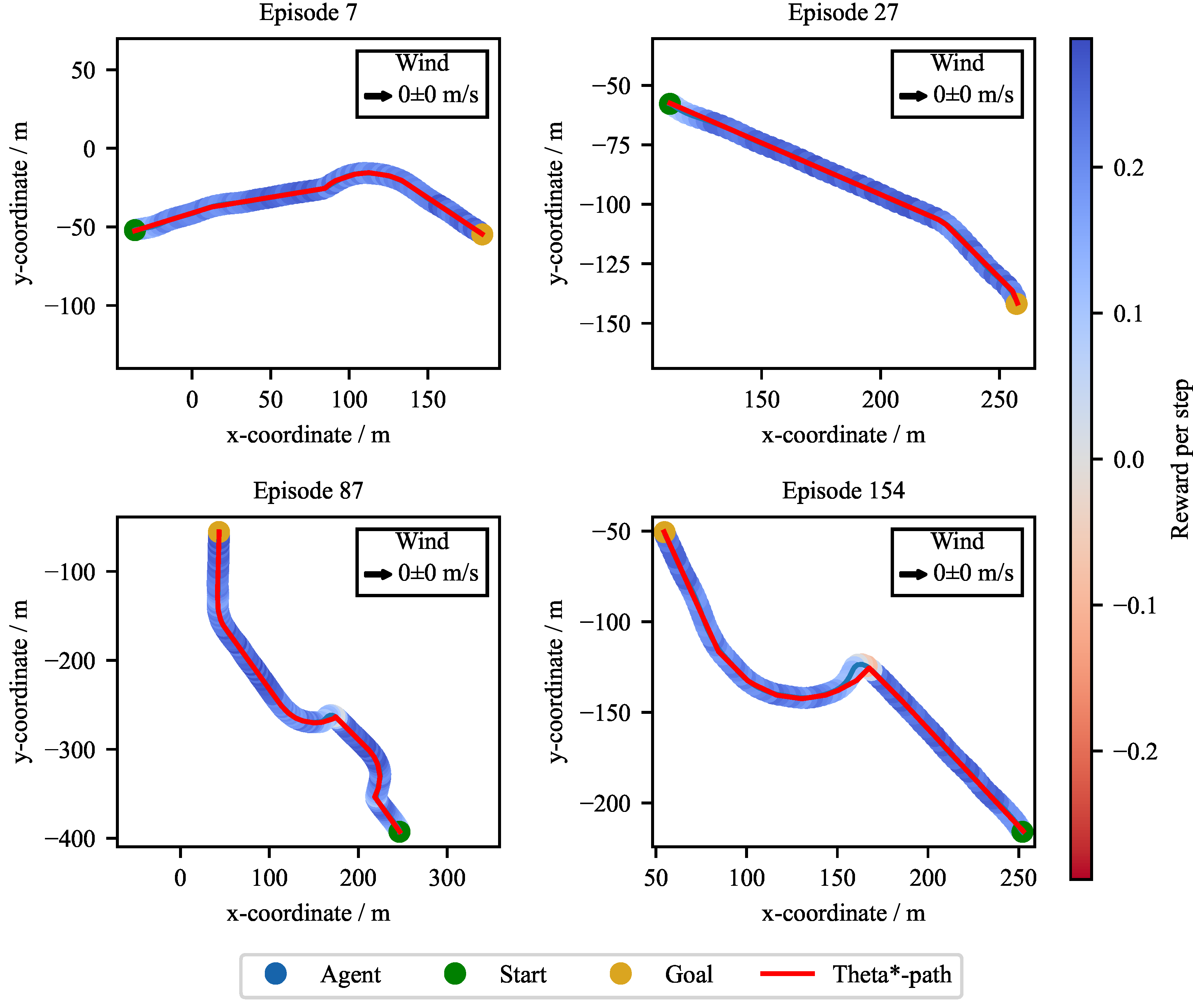
Figure 5 presents four representative trajectory plots obtained during the testing of agent configuration C1_1_1 in the PF1 scenario. The visualizations superimpose the agent’s executed trajectory over the reference path generated by the Theta* algorithm, depicted as a red line. The start and goal positions are identified by green and yellow markers, respectively. To visualize the agent’s performance relative to the optimization criteria, the trajectory color encodes the instantaneous step-wise reward, with blue indicating high reward values and red indicating lower values. To enhance the interpretability of the reward visualization, the final episode reward is excluded from the color map. This allows for a clearer representation of the agent’s step-wise reward progression and supports the identification of critical phases in the maneuvering behavior. The selected episodes demonstrate the agent’s maneuvering capabilities across varying path geometries, including linear segments (Episode 27) and multi-curvature trajectories (Episodes 7, 87 and 154). Qualitatively, the agent maintains proximity to the reference path throughout the majority of the episodes. However, during maneuvers involving sharper path curvature, such as those observed in Episode 154, an increase in CTE is visible. This spatial deviation correlates with a localized reduction in the accumulated reward, visualized by a shift toward lighter or more red hues along the trajectory. This suggests a general sensitivity of the reward function to CTE during complex maneuvers.
Figure 5.
Scenario PF1—Path following without disturbance observation: Wave Adaptive Modular Vehicle (WAMV) trajectories and step rewards from four test simulations of agent C1_1_1 without wind disturbances.
Table 2 summarizes the statistical test results for the PF1 scenario, categorizing episode outcomes by success (goal reached) and failure modes (step limit reached or workspace exited). Agents configured with equally balanced CTE and velocity reward weights, specifically C1_1_1, C1_2_2 and C1_3_3, demonstrate high reliability with goal reaching rates of 100%. In contrast, the configurations C1_3_1 and C1_1_3 failed to reach the target in many episodes (17.0% and 10.5%), with most of the episodes terminating due to the step limit. This indicates that a dominant reward weight results in overly conservative maneuvering that prevents timely goal reaching.
Table 2.
PF1: Statistical test results for multiple agent parameterizations.
The analysis of environmental disturbances distinguishes between agents trained without wind but tested with wind (denoted by the suffix D1) and agents where wind is active during both training and testing (denoted by D2). The PF2 scenario wind variation is used for these agents. Despite not observing wind during training, C1_1_1_D1 achieves a 98.0% success rate, indicating a high degree of robustness. The configuration C1_1_1_D2 records a success rate of 96.0%, with failures primarily attributed to time-outs. This suggests that training under disturbances without explicit observations leads to a more conservative policy; while C1_1_1_D1 maintains a precise kinematic control focusing on reactive compensation of path deviations, C1_1_1_D2 likely interprets the unobserved wind forces as stochastic noise, resulting in reduced velocity and subsequent time-outs.
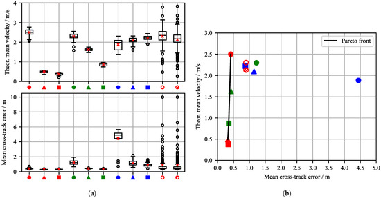
To quantify the impact of reward parameterization on agent performance, Figure 6 illustrates the distribution of two primary metrics: the mean CTE and the theoretical mean velocity. Navigational efficiency is evaluated using the theoretical mean velocity, defined as the total length of the reference path divided by the simulation time required to reach the goal in this episode. This normalization ensures comparability across scenarios with varying path lengths. The path length is used instead of the actual distance traveled, as the aim is to evaluate a normalized goal-reaching time and not the velocity of agents traveling at high speed, but off track. The data include all successful test episodes within the PF1 scenario. The red markers within the box plots denote the arithmetic mean. Exact values of the statistical analysis can be found in Appendix A within Table A1. The theoretical mean velocity across all agent configurations ranges between 0 m/s and 2.5 m/s. A distinct trade-off between path tracking precision and traversal velocity is observable. For instance, configuration C1_2_1 maintains minimal path deviation, but operates at significantly reduced velocities. In contrast, C1_1_2 achieves high velocities ≈ but incurs substantial path deviations, with a CTE of up to 2 m.
Figure 6.
Scenario PF1: Path following without disturbance observation and without wind disturbances. Agent configuration variation: (a) Statistics on mean cross-track error (CTE) and theoretical mean velocity. (b) Theoretical mean velocity over mean cross-track error.
Notably, while configuration C1_2_3 demonstrates a high goal reaching rate (see Table 2), it exhibits considerable variance in both velocity and spatial deviation. Although velocity fluctuations may be operationally acceptable, lateral deviations exceeding 2 m are safety-critical, particularly given the vessel’s length of approximately 5 m. In contrast, the results suggest that a balanced ratio between the CTE penalty and velocity reward—specifically the 1:1 ratio observed in C1_1_1—yields the most favorable outcome. This configuration demonstrates low variance across both metrics, achieving high mean velocities while minimizing path deviation. This trade-off is further analyzed in the scatter plot in Figure 6b, where a Pareto front emerges between the conflicting objectives of minimizing CTE and maximizing velocity. Parameterizations such as C1_1_1 and C1_3_3 populate the optimal region (high velocity, low CTE); while the specific positioning of the resulting Pareto frontier is influenced by our choice of reward functions, it serves as a qualitative indicator of the intrinsic tension between navigational speed and tracking precision.
When C1_1_1 is subjected to unobserved disturbances (test results C1_1_1_D1), the mean CTE of these agents increases by 0.48 m compared to tests without wind C1_1_1, accompanied by an expected increase in variance (values can be found in Table A1). Interestingly, while implicit exposure to wind during training allowed C1_1_1_D2 to achieve a marginally lower mean CTE of compared to for D1, it exhibited a higher standard deviation of . This suggests that while implicit training forces the agent to adopt a more aggressive drift correction policy, it results in less consistent maneuvering and higher susceptibility to episode termination under stochastic peak loads compared to the robust baseline policy of C1_1_1_D1. Both agents (C1_1_1_D1 and C1_1_1_D2) have a wide range of path deviation and speed variance.
In conclusion, the analysis of the PF1 scenario demonstrates that a balanced reward function is critical for optimizing the trade-off between path adherence and navigational efficiency; while agents with disproportionate CTE penalties exhibited overly conservative behavior leading to timeouts and velocity-focused agents sacrificed spatial precision, the configuration C1_1_1 achieved a robust compromise. This parameterization maintained high theoretical mean velocities with minimal spatial deviation and low variance. The agent demonstrated inherent resilience when subjected to unobserved wind disturbances during testing. Consequently, C1_1_1 is selected as the baseline reference for the subsequent PF2 scenario, which investigates the impact of integrating explicit environmental disturbance observations into the agent’s state space.
3.2. Scenario PF2—Path Following with Disturbance Observation
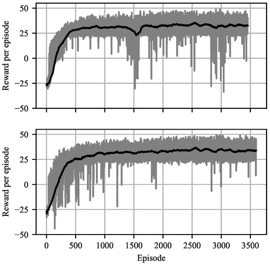
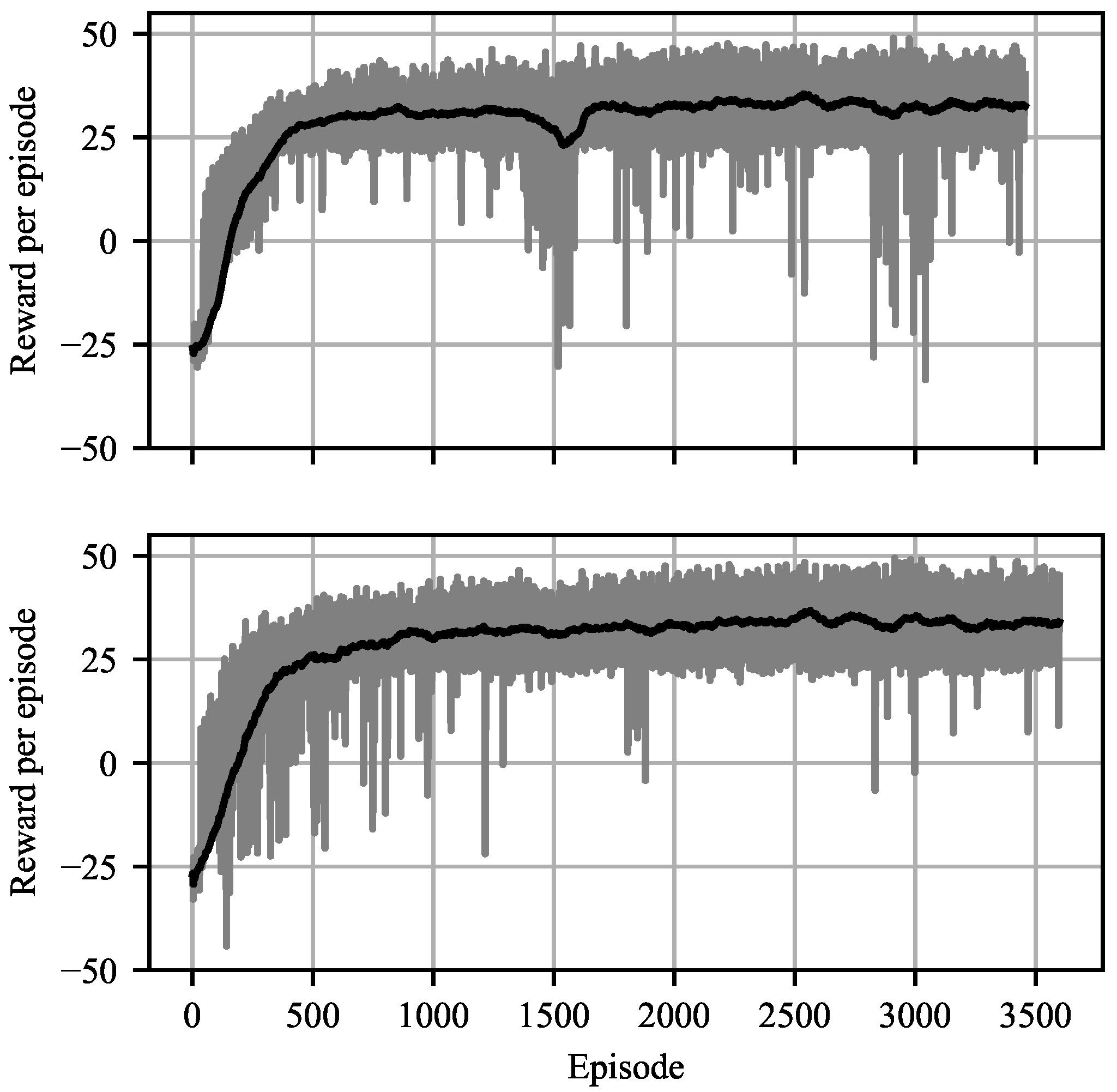
This subsection evaluates the agent’s performance in the PF2 scenario, employing the observation space modifications described in Section 2.2.3 and the scenario generation outlined in Section 2.2.4. A key challenge in PF2 is the effective scheduling of wind velocity variations during training. To address this, two training strategies are compared: a curriculum learning approach (C2_1_1_CL) and a fully randomized approach (C2_1_1). Both strategies utilize an initial learning phase of 100 episodes without environmental disturbances. Figure 7 illustrates the episode reward progression for both strategies. The curriculum-based approach, shown in Figure 7 (top), incrementally increases wind mean and standard deviation values. A distinct performance drop is observable around episode 1450, corresponding to the increasingly harsh wind conditions. This phenomenon is evident in the mean value of the reward, as depicted by the black line in the graph. Following episode 1541, the curriculum concludes and the remaining episodes utilize randomized wind settings, leading to a recovery in the obtained episode reward. Conversely, the randomized strategy shown in Figure 7 (bottom) exposes the agent to the same set of wind vectors, but in a random order immediately after the initial training. While this approach exhibits higher initial volatility (gray curve), it achieves lower episode reward fluctuations toward the end of the training process. Although C2_1_1_CL demonstrates greater stability in the early stages, the randomized approach C2_1_1 ultimately yields superior convergence.
Figure 7.
Visualization of the reward during the training in the PF2 scenario: Comparison of increasing wind speed curriculum learning (C2_1_1_CL, top) versus randomized (C2_1_1, bottom) wind speed variations in training. The gray curve shows the step-wise reward, while the black curve is an average over 100 episodes.
This superiority of the randomized approach is confirmed by the quantitative test results (see Table A1). The randomized approach (C2_1_1) achieves a higher goal reaching rate of 98.0% compared to 97.0% for the curriculum-based agent (C2_1_1_CL) during testing. Furthermore, the randomized strategy demonstrates superior path adherence, with a mean path deviation of 0.73 m compared to 0.92 m for the curriculum approach. The consistency of the performance is also improved, as indicated by a lower standard deviation of the path deviation (0.77 m vs. 0.82 m). Regarding navigational efficiency, both strategies achieve comparable theoretical mean velocities of approximately 2.20 m/s. The randomized approach demonstrates higher consistency, evidenced by a reduced standard deviation of the theoretical mean velocity of 0.37 m/s compared to 0.49 m/s for the curriculum-based agent. Consequently, due to better convergence during training and superior precision during testing, the randomized training strategy is adopted for the subsequent evaluations.
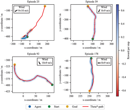
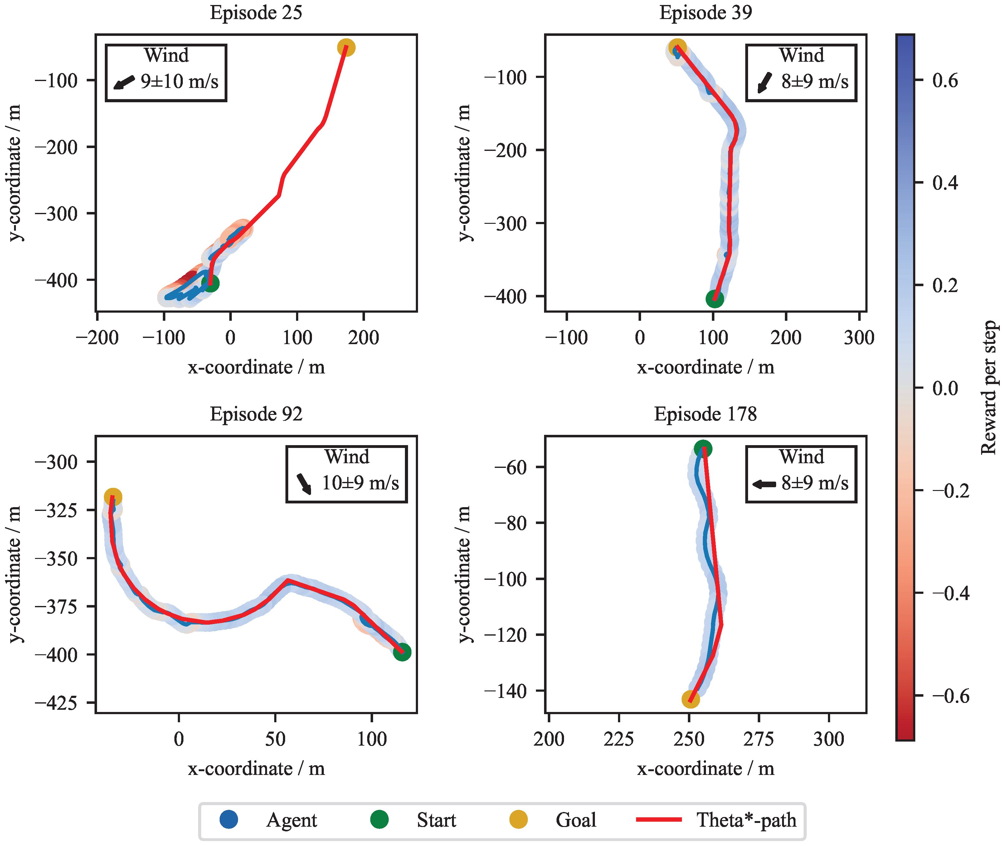
Figure 8 depicts four test episodes for the agent C2_1_1, trained using the randomized strategy. To contextualize the agent’s performance, each subplot includes the active wind parameters, displaying the wind direction vector alongside the mean wind speed and its standard deviation (e.g., 9 m/s mean, 10 m/s standard deviation). All selected episodes feature high-magnitude wind conditions to evaluate disturbance rejection capabilities. The episodes illustrate varying degrees of robustness against environmental forces. Episode 25 represents an unsuccessful attempt where the agent encounters a strong headwind with a mean speed of 9 m/s and a standard deviation of 10 m/s. The trajectory indicates that the vessel is unable to generate sufficient surge force to overcome the opposing environmental resistance, resulting in a timeout before the goal is reached. Episode 178 highlights the kinematic influence of cross-winds. A visible deviation from the reference path aligns with the wind direction, demonstrating a drift effect that the agent compensates for, but does not fully eliminate. In contrast, Episodes 39 and 92 exhibit high precision. Despite similar wind intensities, the agent effectively counteracts the external forces, maintaining a low CTE and adhering closely to the planned trajectory throughout the maneuver.
Figure 8.
Scenario PF2—Path following with disturbance observation: Wave Adaptive Modular Vehicle (WAMV) trajectories and step rewards from four test simulations of agent C2_1_1 with wind disturbances.
Table 3 presents the statistical test results for the PF2 scenario, summarizing the goal reaching rates and failure modes across various agent configurations. Consistently with the PF1 results, agents with high CTE penalties, such as C2_2_1 and C2_3_1, exhibit low success rates (44.5% and 28.5%, respectively) with a high prevalence of timeouts. This confirms that excessive penalization of path deviation leads to overly conservative behavior, preventing the agent from overcoming strong environmental forces to reach the goal within the time limit. Conversely, balanced configurations like C2_1_2, C2_2_2 and C2_3_3 achieve high reliability, with success rates exceeding 98%.
Table 3.
PF2: Statistical test results for multiple agent parameterizations.
A comparison is drawn between the wind-aware agents (PF2) and the baseline agents from the PF1 scenario to assess the value of explicit disturbance observation. The agent C1_1_1_D1, which is trained in a windless environment without wind observations, achieves a success rate of 98.0% when exposed to wind during testing, performing just as good as the best wind-aware configuration C2_1_1 (98.0%). In contrast, the baseline C1_1_1_D2, trained with unobserved wind disturbances, exhibits a lower success rate of 96.0%, with a failure mode dominated by timeouts (3.5%). This indicates that while the blind policy trained in calm water (C1_1_1_D1) generalizes robustly to stochastic environments, the attempt to learn disturbance rejection (C1_1_1_D2) without observation variables results in a less reliable policy that is more prone to reaching the step limit.
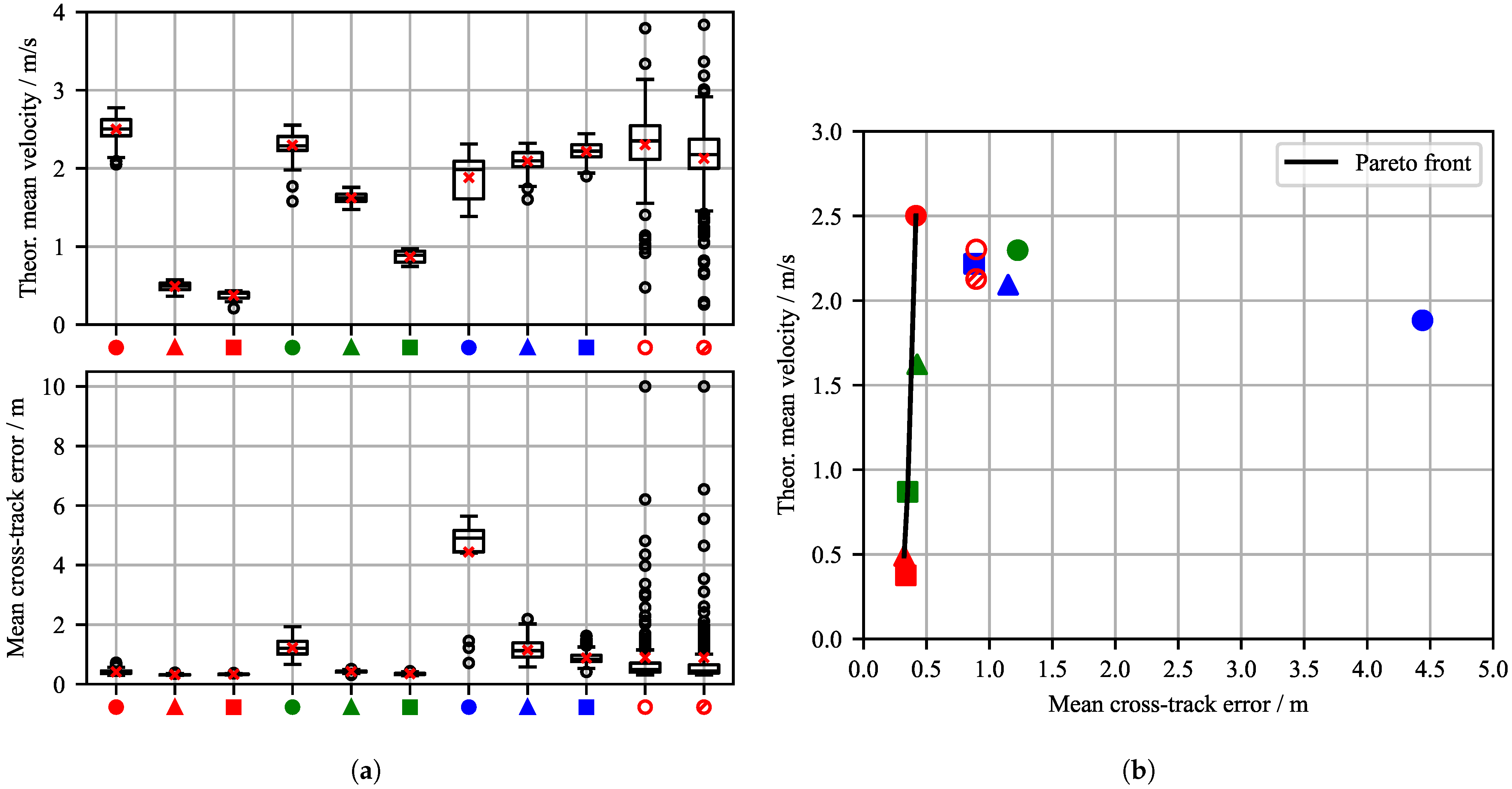
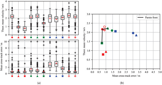
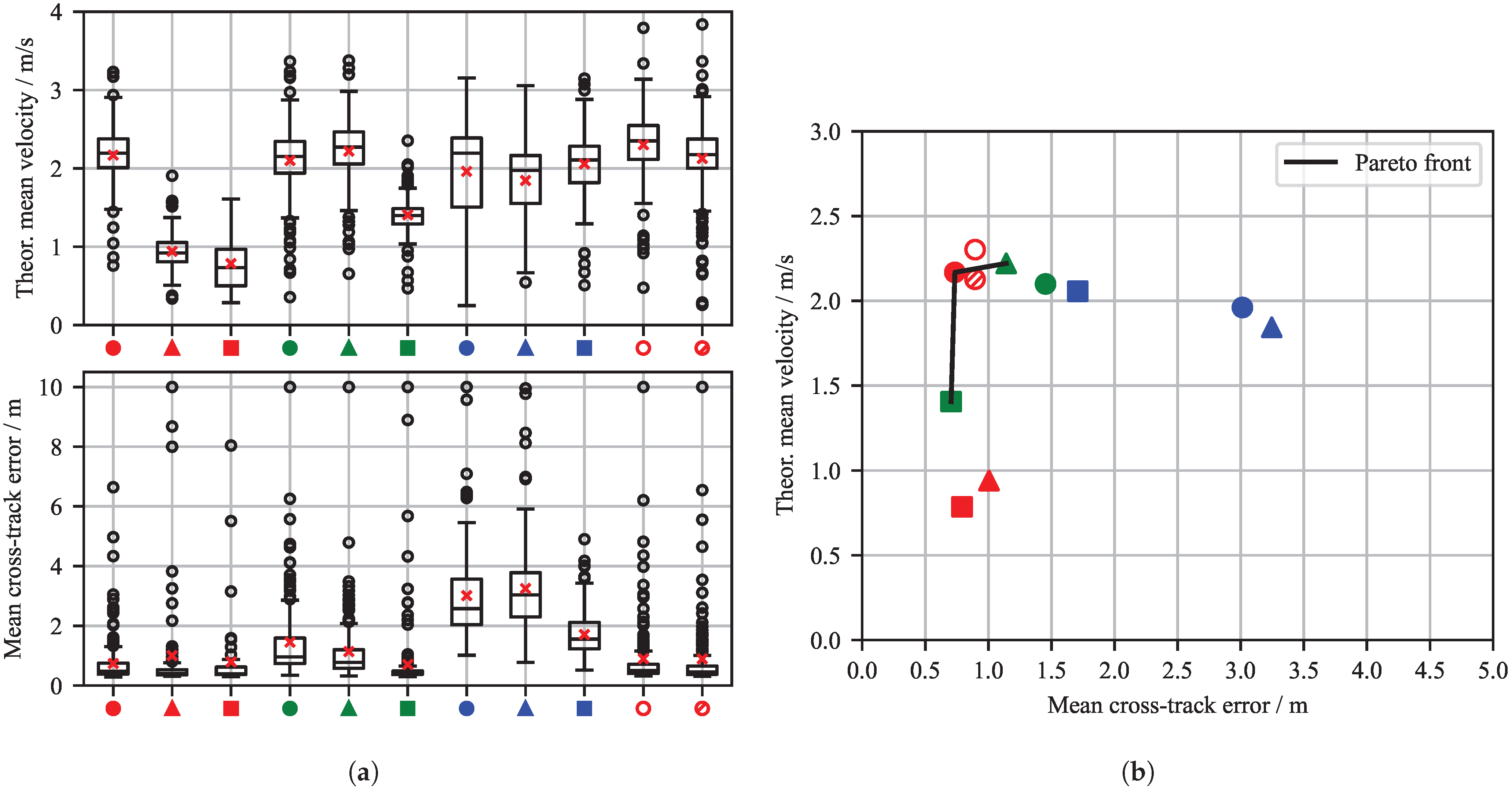
Figure 9 and Table A1 provide a quantitative breakdown of these performance differences. The scatter diagram in Figure 9b delineates the Pareto frontier, highlighting the efficiency limits of the learned policies under disturbance observation. The configuration C2_1_1 resides near the Pareto optimum, offering a favorable compromise with a theoretical mean velocity of 2.17 m/s and a mean CTE of 0.73 m. In comparison, the precision-focused agent C2_3_2 defines the high-accuracy end of the frontier, reducing the mean CTE to 0.70 m but at the cost of a substantial velocity drop to . Notably, parametric unbalanced configurations such as C2_2_1 fall significantly below this frontier, exhibiting both reduced velocities (0.94 m/s) and higher errors (1.01 m), demonstrating that excessive constraints can destabilize the learning process rather than enforcing tighter tracking.
Figure 9.
Scenario PF2—Path following with disturbance observation and with wind disturbances. Agent configuration variation: (a) Statistics on mean cross-track error (CTE) and theoretical mean velocity. (b) Theoretical mean velocity over mean cross-track error.
Configuration C1_1_1_D2 achieves a mean CTE of , which is slightly higher than the PF2 configuration C2_1_1 test results with . The dispersion of the path deviation for the agent without disturbance observation (C1_1_1_D2) is significantly higher in the same test scenario compared to the agent with disturbance observation C2_1_1 ( vs. ). This suggests that explicit wind observation enables the agent to decouple drift compensation from trajectory tracking, allowing for smoother actuation and more consistent path-keeping against environmental forces. To contextualize our findings, we compare the best-performing wind-aware agent C2_1_1 with the learning-based MPC framework by Cheng et al. [40], who reported mean CTE between (weak wave disturbances) and (strong wave disturbances) and mean velocities of to for the WAMV in VRX. Our agent achieves a comparable mean cross-track error with a higher theoretical mean velocity. These results demonstrate that the proposed DRL approach performs within the same dimension as state-of-the-art model-based optimization.
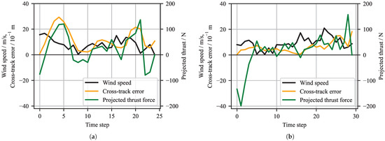
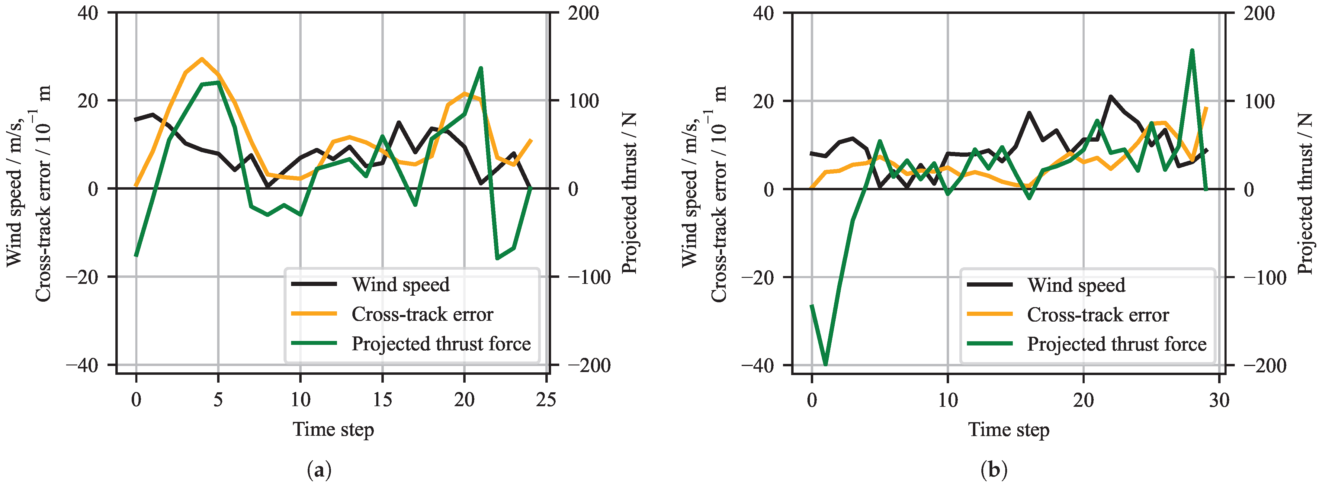
Figure 10 illustrates the disturbance rejection capabilities of both agents in a perpendicular wind scenario. The PF1 agent (Figure 10a) exhibits a distinct lag, increasing thrust only after a path deviation occurs, which confirms the reactive nature of a policy relying solely on kinematic errors. Conversely, the PF2 agent (Figure 10b) demonstrates proactive behavior, synchronizing thrust generation with the wind speed profile to mitigate drift before errors accumulate. Detailed visualizations of the corresponding wind and thrust vectors for the PF2 agent are provided in Appendix A within Figure A1. The figure illustrates the agent’s counteracting behavior against the wind at varying simulation times. While thrust values do not perfectly mirror wind load—as the vessel must overcome additional drag induced by the required sideslip angle (leeway)—the temporal synchronization in PF2 is evident. Thus, integrating wind observations into the control input reduces path deviations and enhances goal-reaching stability.
Figure 10.
Wind speed, CTE and projected thrust force in perpendicular path direction for exemplary test episodes in the (a) PF1 scenario and (b) PF2 scenario.
The performance gains observed in wind-aware agents are attributed to the transition toward a more fully observable Markov Decision Process, which reduces aleatoric uncertainty and simplifies the optimization landscape. Although enhanced observability provides the necessary data, proactive thrust synchronization demonstrated in our results confirms the ability of the policy to learn the underlying physical correlation between wind vectors and the required counter-forces. This combination allows the agent to decouple environmental causes from kinematic effects, facilitating drift compensation before significant cross-track errors accumulate.
4. Conclusions
This study presented a systematic investigation into DRL strategies for autonomous maritime path following under stochastic environmental disturbances. By conducting a comparative analysis of observation spaces and reward functions, we evaluated the agent’s capacity to proactively compensate for wind-induced drift forces. The results demonstrate that integrating the wind vector into the agent’s observation space (PF2) enhances operational stability. While agents trained without wind observation C1_1_1_D2 achieved a success rate, they exhibited increased variance in both CTE and velocity in comparison to C2_1_1. This confirms that providing the policy with environmental states enables a decoupling of disturbance causes from kinematic effects, leading to more precise path adherence. However, the results indicate that the baseline agent (without disturbance observation) is already capable of reliably reaching the destination, suggesting that implicit disturbance rejection is often sufficient for general navigation tasks, though explicit observation offers distinct advantages in precision.
A distinguishing feature of this work is the deliberate focus on the intrinsic comparison of RL configurations rather than a benchmark against classical control schemes (e.g., PID or MPC). Instead of proving the superiority of RL over established model-based methods, this study provides a quantitative framework for understanding how design choices—specifically reward weighting and state observation—influence the learning convergence and emergent behavior of the agent. We identified a distinct Pareto frontier between navigational efficiency and tracking precision, illustrating that a balanced reward function is paramount for preventing overly conservative or erratic behaviors.
Despite the promising results in the simulation, bridging the gap to real-world deployment remains a critical challenge. The training was conducted in the VRX environment, which provides an approximation of maritime physics but inherently simplifies complex hydrodynamic interactions such as wave–current coupling and variable water depths. Consequently, the transferability of the learned policies to a physical WAMV requires further testing. To address the gap, future work must incorporate observations not only for wind, but also for hydrodynamic coefficients and sensor noise. Latency and processing times must also be taken into account when processing real sensor data. Additionally, while this study demonstrates the effectiveness of PPO, exploring alternative DRL algorithms, such as Soft Actor–Critic (SAC) or TD3, could provide further comparative insights into their robustness to disturbances in maritime environments. Furthermore, as the system transitions from simulation to operation, compliance with safety standards becomes mandatory. According to assurance guidelines for autonomous ships, such as those provided by DNV [41], purely learning-based controllers pose challenges for formal verification. Therefore, future research should investigate hybrid architectures that combine the adaptive capabilities of DRL with the safety guarantees of rule-based or barrier-function monitors to ensure safe operation in real-world maritime environments.
Author Contributions
Conceptualization, B.K., D.W., S.-Y.L. and J.A.; methodology, B.K. and D.W.; software, B.K. and D.W.; validation, B.K. and D.W.; formal analysis, B.K.; investigation, B.K.; resources, D.W.; data curation, D.W.; writing—original draft preparation, B.K.; writing—review and editing, B.K., D.W., T.T., T.B., S.-Y.L., D.K. and J.A.; visualization, B.K. and D.W.; supervision, S.-Y.L. and J.A.; project administration, B.K., S.-Y.L. and J.A.; funding acquisition, S.-Y.L. and J.A. All authors have read and agreed to the published version of the manuscript.
Funding
This research received no external funding.
Data Availability Statement
The original contributions presented in this study are included in the article. Further inquiries can be directed to the corresponding author.
Acknowledgments
Computations were performed with computing resources granted by RWTH Aachen University under the project rwth1900.
Conflicts of Interest
The authors declare no conflicts of interest.
Abbreviations
The following abbreviations are used in this manuscript:
| A3C | Asynchronous Advantage Actor–Critic |
| AI | Artificial Intelligence |
| AMV | Autonomous Marine Vehicle |
| APFs | Artificial Potential Fields |
| CTE | Cross-Track Error |
| DDPG | Deep Deterministic Policy Gradient |
| DQN | Deep Q-Network |
| DRL | Deep Reinforcement Learning |
| EKF | Extended Kalman Filter |
| GNC | Guidance Navigation and Control |
| LOS | Line of Sight |
| LSTM | Long Short-Term Memory |
| MPC | Model Predictive Controller |
| PF | Path Following |
| PPO | Proximal Policy Optimization |
| RL | Reinforcement Learning |
| ROS | Robot Operating System |
| RRT | Rapidly Exploring Random Tree |
| SAC | Soft Actor–Critic |
| SLAM | Simultaneous Localization and Mapping |
| TD3 | Twin-Delayed Deep Deterministic Policy Gradient |
| USV | Unmanned Surface Vehicle |
| VRX | Virtual RobotX |
| VTPG | Velocity Toward Path Goal |
| WAMV | Wave Adaptive Modular Vehicle |
Appendix A
The wind and thrust vectors during a test episode of a PF2 agent are visualized in Figure A1. Table A1 contains the mean and standard deviation of the theoretical mean velocity and cross-track error (CTE) for all agent parameterizations.
Figure A1.
Wind and thrust vectors for an exemplary test episode in the PF2 scenario. The blue dots indicate the WAMV’s intermediate positions.
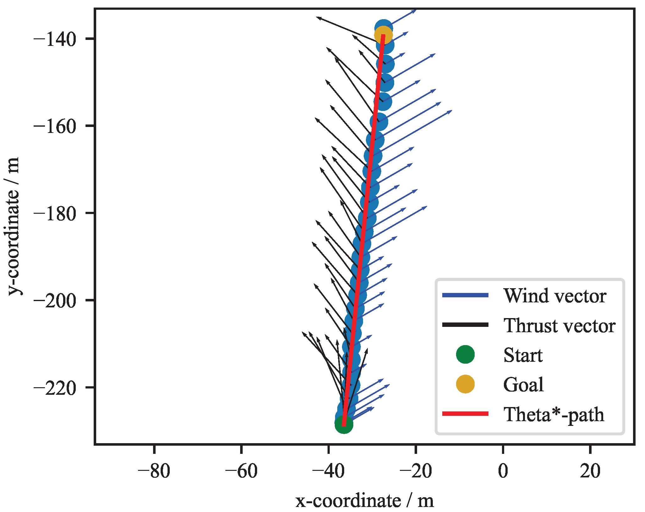
Table A1.
Mean and standard deviation (SD) of the theoretical mean velocity and cross-track error for all agent parameterizations.
References
- Liu, Z.; Zhang, Y.; Yu, X.; Yuan, C. Unmanned surface vehicles: An overview of developments and challenges. Annu. Rev. Control 2016, 41, 71–93. [Google Scholar] [CrossRef] [Scilit]
- Krautwig, B.; Wans, D.; Li, L.; Temmen, T.; Koch, L.; Eisenbarth, M.; Andert, J. Navigating the Trade-Offs: A Quantitative Analysis of Reinforcement Learning Reward Functions for Autonomous Maritime Collision Avoidance. J. Mar. Sci. Eng. 2025, 13, 2233. [Google Scholar] [CrossRef] [Scilit]
- Siciliano, B.; Khatib, O. (Eds.) Springer Handbook of Robotics; Springer: Berlin/Heidelberg, Germany, 2008. [Google Scholar] [CrossRef] [Scilit]
- Chen, C.S.; Lin, C.J.; Lai, C.C.; Lin, S.Y. Velocity Estimation and Cost Map Generation for Dynamic Obstacle Avoidance of ROS Based AMR. Machines 2022, 10, 501. [Google Scholar] [CrossRef] [Scilit]
- Ferguson, D.; Likhachev, M. Efficiently Using Cost Maps For Planning Complex Maneuvers. In Proceedings of International Conference on Robotics and Automation Workshop on Planning with Cost Maps; IEEE: Piscataway, NJ, USA, 2008. [Google Scholar]
- Racinskis, P.; Arents, J.; Greitans, M. Constructing Maps for Autonomous Robotics: An Introductory Conceptual Overview. Electronics 2023, 12, 2925. [Google Scholar] [CrossRef] [Scilit]
- Thrun, S. Robotic mapping: A survey. In Exploring Artificial Intelligence in the New Millennium; Morgan Kaufmann Publishers Inc.: San Francisco, CA, USA, 2003; pp. 1–35. [Google Scholar]
- Yi, C.; Jeong, S.; Cho, J. Map Representation for Robots. Smart Comput. Rev. 2012, 2, 18–27. [Google Scholar] [CrossRef] [Scilit]
- Macenski, S.; Moore, T.; Lu, D.V.; Merzlyakov, A.; Ferguson, M. From the desks of ROS maintainers: A survey of modern & capable mobile robotics algorithms in the robot operating system 2. Robot. Auton. Syst. 2023, 168, 104493. [Google Scholar] [CrossRef] [Scilit]
- Sanchez, M.; Morales, J.; Martínez, J.; Fernández-Lozano, J.; Garcia, A. Automatically Annotated Dataset of a Ground Mobile Robot in Natural Environments via Gazebo Simulations. Sensors 2022, 22, 5599. [Google Scholar] [CrossRef] [Scilit]
- Souissi, O.; Benatitallah, R.; Duvivier, D.; Artiba, A.; Belanger, N.; Feyzeau, P. Path planning: A 2013 survey. In Proceedings of the 2013 International Conference on Industrial Engineering and Systems Management (IESM), Rabat, Morocco, 28–30 October 2013; Curran Associates, Inc.: Red Hook, NY, USA, 2013; pp. 1–8. [Google Scholar]
- LaValle, S.M. Planning Algorithms, reprinted. ed.; Cambridge University Press: New York, NY, USA, 2014; p. cop. 2006. [Google Scholar]
- Karaman, S.; Frazzoli, E. Sampling-based algorithms for optimal motion planning. Int. J. Robot. Res. 2011, 30, 846–894. [Google Scholar] [CrossRef] [Scilit]
- Loe, Ø. Collision Avoidance Concepts for Marine Surface Craft. Trondheim 2007, 19, 111. [Google Scholar]
- Alessandretti, A.; Aguiar, A.P.; Jones, C.N. Trajectory-tracking and path-following controllers for constrained underactuated vehicles using Model Predictive Control. In Proceedings of the 2013 European Control Conference (ECC), Zurich, Switzerland, 17–19 July 2013; IEEE: Piscataway, NJ, USA, 2013; pp. 1371–1376. [Google Scholar] [CrossRef] [Scilit]
- Thyri, E.H.; Breivik, M. Collision avoidance for ASVs through trajectory planning: MPC with COLREGs-compliant nonlinear constraints. Model. Identif. Control A Nor. Res. Bull. 2022, 43, 55–77. [Google Scholar] [CrossRef] [Scilit]
- Kamel, M.S.; Stastny, T.; Alexis, K.; Siegwart, R. Model Predictive Control for Trajectory Tracking of Unmanned Aerial Vehicles Using Robot Operating System. In Robot Operating System (ROS); Springer: Berlin/Heidelberg, Germany, 2017. [Google Scholar] [CrossRef] [Scilit]
- Wallace, M.T.; Streetman, B.; Lessard, L. Model Predictive Planning: Trajectory Planning in Obstruction-Dense Environments for Low-Agility Aircraft. arXiv 2024, arXiv:2309.16024v2. [Google Scholar] [CrossRef] [Scilit]
- Li, Z.; Sun, J. Disturbance Compensating Model Predictive Control With Application to Ship Heading Control. IEEE Trans. Control. Syst. Technol. 2012, 20, 257–265. [Google Scholar] [CrossRef] [Scilit]
- Moser, M.M.; Huang, M.; Abel, D. Model Predictive Control for Safe Path Following in Narrow Inland Waterways for Rudder Steered Inland Vessels*. In Proceedings of the 2023 European Control Conference (ECC), Bucharest, Romania, 13–16 June 2023; IEEE: Piscataway, NJ, USA, 2023; pp. 1–6. [Google Scholar] [CrossRef] [Scilit]
- Wang, Y.; Tong, H.; Fu, M. Line-of-sight guidance law for path following of amphibious hovercrafts with big and time-varying sideslip compensation. Ocean Eng. 2019, 172, 531–540. [Google Scholar] [CrossRef] [Scilit]
- Fossen, T.I.; Breivik, M.; Skjetne, R. Line-of-sight path following of underactuated marine craft. IFAC Proc. Vol. 2003, 36, 211–216. [Google Scholar] [CrossRef] [Scilit]
- Xia, J.; Zhu, X.; Liu, Z.; Luo, Y.; Wu, Z.; Wu, Q. Research on Collision Avoidance Algorithm of Unmanned Surface Vehicle Based on Deep Reinforcement Learning. IEEE Sens. J. 2023, 23, 11262–11273. [Google Scholar] [CrossRef] [Scilit]
- Johansen, T.A.; Fossen, T.I.; Berge, S.P. Constrained Nonlinear Control Allocation with Singularity Avoidance Using Sequential Quadratic Programming. IEEE Trans. Control Syst. Technol. 2004, 12, 211–216. [Google Scholar] [CrossRef] [Scilit]
- Lorenz, U. Reinforcement Learning: Aktuelle Ansätze Verstehen–Mit Beispielen in Java und Greenfoot, 2nd ed.; Springer: Berlin/Heidelberg, Germany, 2024. [Google Scholar] [CrossRef] [Scilit]
- Chen, Z.; Bao, T.; Zhang, B.; Wu, T.; Chu, X.; Zhou, Z. Deep Reinforcement Learning Methods for USV Control: A Review. In Proceedings of the 2023 China Automation Congress (CAC), Chongqing, China, 17–19 November 2023; IEEE: Piscataway, NJ, USA, 2023; pp. 1526–1531. [Google Scholar] [CrossRef] [Scilit]
- Li, S.; Ji, Y.; Liu, J.; Bai, Z.; Hu, J.; Gao, Q. Global Path Planning of Unmanned Surface Vehicles Based on Deep Q Network. In Proceedings of the 2024 43rd Chinese Control Conference (CCC), Kunming, China, 28–31 July 2024; IEEE: Piscataway, NJ, USA, 2024; pp. 3827–3832. [Google Scholar] [CrossRef] [Scilit]
- Zhao, J.; Wang, P.; Li, B.; Bai, C. A DDPG-Based USV Path-Planning Algorithm. Appl. Sci. 2023, 13, 10567. [Google Scholar] [CrossRef] [Scilit]
- Zhong, W.; Li, H.; Meng, Y.; Yang, X.; Feng, Y.; Ye, H.; Liu, W. USV path following controller based on DDPG with composite state-space and dynamic reward function. Ocean Eng. 2022, 266, 112449. [Google Scholar] [CrossRef] [Scilit]
- Deraj, R.; Kumar, R.S.; Alam, M.S.; Somayajula, A. Deep reinforcement learning based controller for ship navigation. Ocean Eng. 2023, 273, 113937. [Google Scholar] [CrossRef] [Scilit]
- Qu, X.; Jiang, Y.; Zhang, R.; Long, F. A Deep Reinforcement Learning-Based Path-Following Control Scheme for an Uncertain Under-Actuated Autonomous Marine Vehicle. J. Mar. Sci. Eng. 2023, 11, 1762. [Google Scholar] [CrossRef] [Scilit]
- Dong, Z.; Chen, L.; Huang, Y.; Chen, P.; Mou, J. Model-based Reinforcement Learning for Ship Path Following with Disturbances. IFAC-PapersOnLine 2024, 58, 247–252. [Google Scholar] [CrossRef] [Scilit]
- Raffin, A.; Hill, A.; Gleave, A.; Kanervisto, A.; Ernestus, M.; Dormann, N. Stable-Baselines3: Reliable Reinforcement Learning Implementations. J. Mach. Learn. Res. 2021, 22, 1–8. [Google Scholar]
- Brockman, G.; Cheung, V.; Pettersson, L.; Schneider, J.; Schulman, J.; Tang, J.; Zaremba, W. Openai gym. arXiv 2016, arXiv:1606.01540. [Google Scholar] [CrossRef] [Scilit]
- Bingham, B.; Agüero, C.; McCarrin, M.; Klamo, J.; Malia, J.; Allen, K.; Lum, T.; Rawson, M.; Waqar, R. Toward Maritime Robotic Simulation in Gazebo. In Proceedings of the OCEANS 2019 MTS/IEEE SEATTLE, Seattle, WA, USA, 27–31 October 2019; IEEE: Piscataway, NJ, USA, 2019; pp. 1–10. [Google Scholar] [CrossRef] [Scilit]
- Quigley, M.; Gerkey, B.; Conley, K.; Faust, J.; Foote, T.; Leibs, J.; Berger, E.; Wheeler, B.; Ng, A. ROS: An open-source Robot Operating System. In Proceedings of the ICRA Workshop on Open Source Software; IEEE: Piscataway, NJ, USA, 2009; Volume 3, p. 5. [Google Scholar]
- Daniel, K.; Nash, A.; Koenig, S.; Felner, A. Theta*: Any-Angle Path Planning on Grids. J. Artif. Intell. Res. 2010, 39, 533–579. [Google Scholar] [CrossRef] [Scilit]
- Abouelazm, A.; Michel, J.; Zöllner, J. A Review of Reward Functions for Reinforcement Learning in the context of Autonomous Driving. In Proceedings of the 2024 IEEE Intelligent Vehicles Symposium (IV), Jeju Island, Republic of Korea, 2–5 June 2024; IEEE: Piscataway, NJ, USA, 2024. [Google Scholar] [CrossRef] [Scilit]
- Florensa, C.; Held, D.; Wulfmeier, M.; Zhang, M.; Abbeel, P. Reverse Curriculum Generation for Reinforcement Learning. arXiv 2018, arXiv:1707.05300. [Google Scholar] [CrossRef] [Scilit]
- Cheng, M.; Yao, J.; Ren, Q. A Model Predictive Control Approach for USV Autonomous Cruising via Disturbance Learning. In Proceedings of the 2024 IEEE 18th International Conference on Control & Automation (ICCA), Reykjavík, Iceland, 18–21 June 2024; IEEE: Piscataway, NJ, USA, 2024; pp. 988–993. [Google Scholar] [CrossRef] [Scilit]
- DNV. Class Guideline: Autonomous and Remotely Operated Ships (DNV-CG-0264); Technical Report; DNV GL: Houston, TX, USA, 2021. [Google Scholar]



Disclaimer/Publisher’s Note: The statements, opinions and data contained in all publications are solely those of the individual author(s) and contributor(s) and not of MDPI and/or the editor(s). MDPI and/or the editor(s) disclaim responsibility for any injury to people or property resulting from any ideas, methods, instructions or products referred to in the content. |
© 2026 by the authors. Licensee MDPI, Basel, Switzerland. This article is an open access article distributed under the terms and conditions of the Creative Commons Attribution (CC BY) license.