


Abstract
Sea surface temperature (SST) modes of climate variability in the South Atlantic Ocean remain a challenging topic. To improve the understanding of this subject, this study assesses the influence of two commonly discussed SST variability modes, the South Atlantic Dipole (SAD) and the Southwestern South Atlantic (SWSA), on South America (SA) during the present-day climate conditions and discusses, based on the previous literature, their development. Complementing previous analyses based on annual or seasonal scales, the analysis is performed at the monthly scale, given its relevance for subseasonal-to-seasonal (S2S) forecasts. Empirical Orthogonal Function (EOF) analysis was applied to standardized monthly SST anomalies relative to the period 1991–2020, using data from the Extended Reconstructed Sea Surface Temperature (ERSST). After characterizing the SAD and SWSA modes, composites of different variables, such as precipitation anomalies, were constructed for the different phases of each pattern. The results show that the SAD is the dominant mode of SST variability, mainly influencing tropical latitudes by modulating the Intertropical Convergence Zone (ITCZ). During its positive (negative) phase, the ITCZ shifts southward (northward). In contrast, the SWSA exhibits a more localized subtropical–extratropical structure, characterized by SST anomalies along the south–southeastern coast of Brazil, and is closely associated with variability in the South Atlantic Convergence Zone (SACZ). The relationship between the SWSA and SACZ appears strong during the austral extended summer, when warmer waters during the positive (negative) SWSA phase are associated with wetter (drier) conditions over southeastern SA and drier (wetter) conditions over the continental and oceanic branches of the SACZ.
1. Introduction
In the mid-to-late 1990s, growing attention was directed toward understanding the modes of sea surface temperature (SST) variability in the South Atlantic Ocean (SAO), although their impacts on South American climate received comparatively little emphasis. Among the pioneering studies in this context are Venegas et al. [1,2], who provided one of the first descriptions of the SST variability using multivariate statistical techniques. Principal component analysis (PCA, also known as Empirical Orthogonal Function—EOF [3]) and singular value decomposition (SVD) were the multivariate techniques applied by these authors. EOF analysis was used separately for the SST and mean sea level pressure (MSLP) variables, while SVD was employed to examine coupled variability between the two fields.
Differences among studies regarding the leading EOF modes of SST variability in the SAO (Table 1) have been largely attributed to methodological choices, such as the data preprocessing, spatial domain, and temporal period. According to Nnamchi et al. [4], the different EOF ordering of the tropical–subtropical dipole mode in Morioka et al. [5] and Nnamchi et al. [6] arises from such methodological differences, which alter the variance distribution and, consequently, the statistical ranking of the modes. Similar conclusions were drawn by Kayano et al. [7], who argued that SST standardization was the main source of discrepancies between their results and those of Nnamchi et al. [6].
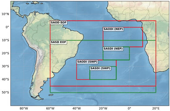
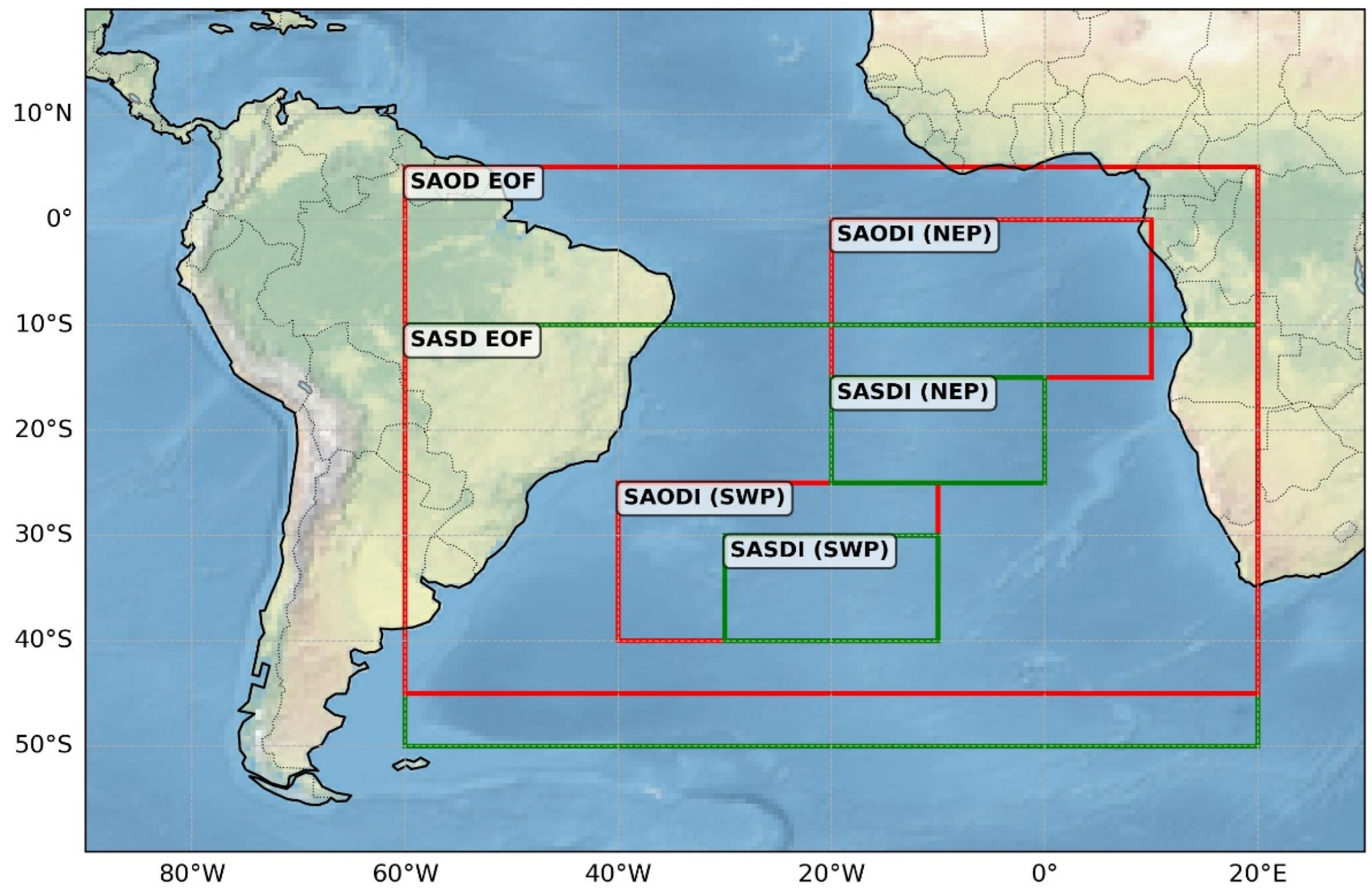
Despite these differences, the existing literature on the main SST patterns in the SAO, summarized in Table 1, consistently identifies a meridional SST dipole characterized by anomalies of opposite sign between the tropical and subtropical basins. This dipole has been identified under different EOF orders (e.g., as the first or second leading mode) and described using different terminology, depending on the methodological choices adopted in each analysis. It has been referred to as the South Atlantic Dipole (SAD) [7,8], the South Atlantic Subtropical Dipole (SASD) [5], and the South Atlantic Ocean Dipole (SAOD) [6]. Based on the leading EOF patterns, Morioka et al. [5] and Nnamchi et al. [6] defined indices that emphasize distinct seasonal expressions of the meridional dipole. The spatial domains and geographic poles used to define the SAOD and SASD indices in previous studies are illustrated in Figure 1. For clarity, in the present study, the term SAD is used to refer to the tropical–subtropical meridional SST pattern.
Figure 1.
Spatial domains of the SAOD (red) and SASD (green) EOF modes, along with the geographic poles used to compute the SAODI and SASDI indices. For SAODI, the poles are NEP (10° E–20° W, 0°–15° S) and SWP (10° W–40° W, 25° S–40° S), and for SASDI, the poles are NEP (0°–20° W, 15° S–25° S) and SWP (10° W–30° W, 30° S–40° S). The SAOD domain is the same as used in this work.
Nnamchi et al. [4] demonstrated that the SASD and SAOD represent different manifestations of the same meridional mode, with the SASD exhibiting its strongest expression during austral summer, when air–sea coupling over the subtropical basin amplifies SST gradients, and the SAOD peaking in austral winter, associated with the maximum meridional thermal gradient and intensified trade-wind forcing. These seasonal differences do not undermine the physical robustness of the mode, but rather reflect the sensitivity of EOF-based methods to the background climatological state and analysis design. We highlight that the objective of the studies by Nnamchi et al. [6] and Morioka et al. [5] was not to provide a comprehensive description of all modes of SST variability in the SAO, but rather to investigate the tropical–subtropical dipole and its seasonal manifestations. Consequently, their EOF analyses were designed to isolate this specific mode, and other SST patterns that may emerge at higher EOF orders or under different temporal scales were outside the scope of those studies.
An important distinction among studies concerns the adopted sign convention. In the SASD framework, the positive phase is characterized by cold SST anomalies in the tropical pole and warm anomalies in the subtropical pole, whereas the SAOD definition adopts the opposite configuration. Because both conventions coexist in the literature, inconsistent interpretations may arise if the sign definition is not explicitly stated. Therefore, in this study, the positive (negative) phase of the SAD is defined as positive (negative) SST anomalies in the tropical core and negative (positive) anomalies in the subtropical core. When results from previous studies are discussed, their original definitions are adjusted, when necessary, to conform to this convention.
Table 1.
Summary of South Atlantic variability modes derived from SST and MSLP variables described in previous studies, including analysis periods, spatial domains, and associated dipole structures. MSLP-based results are shown in italics. “Dipole T–S” denotes a tropical–subtropical dipole, and “Dipole S–H” a subtropical–high latitude dipole.
Beyond the extensively documented tropical–subtropical dipole, the literature also reports SST variability patterns that are not captured when the analysis is explicitly focused on the SAD. Previous studies have identified an additional mode of SST variability in the SAO characterized by a subtropical–high latitude structure. Kayano et al. [8] termed this pattern the Southwestern South Atlantic (SWSA) mode, which emerged as EOF3 in their analysis. This mode is characterized by an SST anomalous center in the southwestern SAO near 30° S, 40° W, accompanied by weaker anomalies of opposite sign over the southern mid-latitudes.
Unlike the SAD, which is primarily associated with large-scale meridional SST gradients spanning the tropical and subtropical SAO, the SWSA exhibits a more localized subtropical–extratropical structure. Kayano et al. [8] emphasized that this mode does not correspond to the dominant tropical–subtropical dipole described in earlier studies; rather, it resembles the subtropical–high latitude dipole previously identified by Palastanga et al. [9].
In this study, the SAD and SWSA modes are treated as distinct SST variability patterns based on their spatial structure and latitudinal extent. The SAD is defined as a meridional dipole spanning the tropical and subtropical SAO, characterized by SST anomalies of opposite sign between these two regions and associated with large-scale meridional SST gradients. In contrast, the SWSA is defined as a subtropical–high latitude pattern, with its main SST anomaly center located in the southwestern SAO, near the southeastern coast of SA, and weaker anomalies of opposite sign toward higher southern latitudes. Unlike the SAD, which reflects basin-scale tropical–subtropical variability, the SWSA exhibits a more regional structure confined to the subtropical and extratropical SAO.
Based on the long-term experience of the Climate Studies Group of the University of São Paulo (GrEC–USP), the continuous South American climate monitoring has highlighted that, in addition to the SAD, SST anomalies near the south–southeastern Brazilian coast may also influence continental precipitation. These anomalies resemble the subtropical–high latitude dipole structure described as the SWSA mode [8]. From a forecasting perspective, this interpretation is particularly relevant, as the identification of monthly SWSA-like SST patterns may serve as an indicator of the dominant atmospheric systems affecting the eastern flank of South America (SA), thereby contributing to improved subseasonal-to-seasonal climate predictions. Besides this, the SWSA mode has received considerably less attention in the literature, and its physical interpretation remains less consolidated.
Available evidence suggests that the SWSA may primarily reflect an oceanic response to atmospheric forcing rather than a coupled ocean–atmosphere mode [11,12]. One line of evidence involves its relationship with the Southern Annular Mode (SAM). During the SAM positive phase, enhanced anticyclonic circulation south of Uruguay favors clear-sky conditions and ocean warming, while cyclonic anomalies near southeastern Brazil increase cloud cover, reduce incoming solar radiation, and cool the ocean surface. Previous studies have also shown that such SST anomalies are more likely a consequence, rather than a cause, of South Atlantic Convergence Zone (SACZ) intensification [13]. Drumond and Ambrizzi [11], in their analysis of the severe South American drought of 2001, identified an SST anomaly pattern resembling the SWSA dipole, in which warm water near southeastern Brazil predominates; however, numerical experiments using an atmospheric general circulation model did not reproduce the observed precipitation anomalies when forced by SAO SST conditions. This result supports the hypothesis that, in subtropical regions, atmospheric circulation anomalies play a dominant role in shaping SST variability.
Few studies have investigated the relationship between SAO SST variability modes and South American precipitation. Kayano et al. [8] analyzed the influence of the SAD with and without different El Niño–Southern Oscillation (ENSO) phases on rainfall over SA. Their results indicate that the SAD-related precipitation anomalies are weakly modulated by the ENSO. Focusing on ENSO-neutral conditions, Bombardi et al. [7] showed that the negative phase of the SAD is associated with positive precipitation anomalies over the South Atlantic Convergence Zone (SACZ). Similarly, Nnamchi et al. [6,14] found correlations between the ocean precipitation and the SAD domain, indicating that higher volumes of precipitation are associated with colder waters. Evidence for the influence of the SWSA mode on SA continental precipitation remains more limited. Kayano et al. [8] reported that SWSA-related SST anomalies contribute to rainfall variability over southern and southeastern SA, particularly when combined with ENSO phases. However, the physical mechanisms linking the SWSA mode to precipitation anomalies are still not fully understood, and existing results suggest that this mode may primarily reflect atmospheric forcing acting on the ocean rather than a fully coupled ocean–atmosphere process.
Over the last decades, changes in the mean state of the climate system have added complexity to the interpretation of climate variability and its associated modes. Several studies have pointed out that ongoing climate change can alter atmospheric circulation patterns and, consequently, the expression, intensity, and spatial structure of climate variability modes and their teleconnections [15]. In this context, results derived from long-term historical records may not fully represent the characteristics of the present-day climate. As discussed by Barreiro [15], shifts in the background climate can modify the interaction between the atmosphere and the ocean, affecting both variability and predictability. In addition, L’Heureux [16] emphasized that the choice of the reference climatological period plays a critical role in the identification and characterization of climate phenomena, particularly when using anomaly-based methods such as EOF analysis. Different climatological baselines can lead to changes in the variance distribution and, consequently, in the relative importance of the identified modes.
Despite these considerations, most previous studies addressing SAO SST variability modes rely on older climatological baseline periods or extended time series that include substantially different background climate conditions. As a result, the extent to which the identified modes and their associated impacts are representative of the current climate remains an open question. Bier [17] has shown that the characteristics of the SAD exhibit low frequency variability, with changes in spatial structure and intensity over time, supporting the use of a more recent climatological period in our study. Focusing on a recent period may therefore provide a clearer picture of how SAO SST variability modes operate under present-day atmospheric and oceanic conditions. This approach is particularly relevant when the objective is to support subseasonal-to-seasonal (S2S) climate applications, which depend on an accurate representation of contemporary climate variability rather than long-term historical behavior. Accordingly, given the limited number of studies addressing the influence of SAO SST variability modes on South American precipitation under present-climate conditions (1991–2020), and the scarcity of analyses performed at the monthly-calendar scale, this study investigates how the South American climate responds to different phases of two SST patterns: the SAD, characterized by a tropical–subtropical meridional structure, and the SWSA pattern, which exhibits a subtropical–high-latitude configuration.
2. Materials and Methods
2.1. Study Area and Datasets
The study area is the SAO, and our EOF domain follows Nnamchi et al. [6] (Figure 1), ensuring an adequate representation of the South Atlantic Subtropical Anticyclone (SASA) action area throughout the year. Monthly data of the SST, precipitation, MSLP, horizontal wind components at 10 m height and at 850 hPa, and geopotential height at 200 hPa and 1000 hPa were used. While the EOF and rotated EOF (REOF) are computed using the World Meteorological Organization’s most recent climatological period (January 1991–December 2020), the other statistical analyses are extended to cover January 1980–September 2025 in order to increase the sample size used in this study.
The monthly grid SST dataset is the Extended Reconstructed Sea Surface Temperature (ERSST) [18] version 5 (https://www.ncei.noaa.gov/pub/data/cmb/ersst/v5/netcdf/, accessed on 1 December 2025), with a horizontal resolution of 2° × 2°. This dataset is constructed using different data sources: SST from ICOADS (ships and buoys) and profiling floats from Argo Float GDAC; and ice concentration from HadISST2 (1854–2015) and NCEP (2016–present).
The monthly mean precipitation (mm day−1) data were obtained from the Global Precipitation Climatology Project (GPCP) version 2.3 of the National Oceanic and Atmospheric Administration (NOAA) [19]. These data have a horizontal resolution of 2.5° × 2.5° and can be accessed at https://psl.noaa.gov/data/gridded/data.gpcp.html (accessed on 1 December 2025).
The monthly MSLP, horizontal wind components (zonal, u, and meridional, v) and geopotential height were obtained from the ERA5 reanalysis [20]. ERA5 has a horizontal resolution of 0.25° × 0.25°, and data access is available through the Climate Data Store (CDS): https://cds.climate.copernicus.eu/datasets/reanalysis-era5-single-levels-monthly-means?tab=overview (accessed on 1 December 2025).
As in this study we are interested in broad patterns, ERA5 was interpolated to a grid of 2° × 2°. The Niño 3.4 SST index related to the climatological period (1991–2020) was obtained from the Teleconnection Index Online Tool available at https://app-indice.streamlit.app/ [21] (accessed on 1 December 2025). Seasonal definitions follow the Southern Hemisphere calendar.
2.2. Preprocessing Data and Statistical Tools
2.2.1. Data Preparation
Before performing the SST EOF analysis, the annual cycle is removed from the SST dataset by subtracting the monthly climatology (1991–2020) from each corresponding month. The resulting anomalies are then standardized by dividing them by their respective monthly standard deviations. In this study, the EOF analysis is conducted separately for each calendar month (i.e., January, February, etc.), meaning that a distinct EOF decomposition is obtained for each monthly time series. To ensure equal area weighting, the gridded data is weighted by the square root of the cosine of the latitude, the procedure following [22,23,24]. Finally, the data are arranged into a 2D matrix in S-mode, with grid points placed in the columns and time in the rows [25]. Therefore, the eigenvector will describe the spatial pattern of the variability modes.
2.2.2. EOF Technique
The modes of SST variability are obtained through the application of the EOF technique [26,27] to the prepared data for the domain, the same as Nnamchi et al. [6], in the red box (SAOD EOF) as shown in Figure 1. The EOF analysis is based on matrix diagonalization from linear algebra. Specifically, from the covariance matrix we get a diagonal matrix, which corresponds to the eigenvalues, and with additional algebra, the eigenvectors’ matrix. The number of eigenvalues and eigenvectors is equal to the number of columns of the prepared data, which are considered as variables in the analysis. The sum of the eigenvalues is equal to the sum of the variances of these variables. The eigenvectors are also referred to as EOFs, principal components, leading modes, or modes. Here we will use EOFs and modes interchangeably.
At this stage, the main modes of variability in the SST anomaly field have been identified through EOF analysis. Each EOF mode is associated with a temporal coefficient (often referred to as the coefficient time series, z-score, or loading). This coefficient time series provides one value per timestep and can be interpreted as an index of how strongly the SST anomaly field at that timestep projects onto the spatial EOF pattern. In other words, the index indicates whether the SST anomalies at a given timestep resemble the mode under analysis, represent its inverse, or show little to no similarity. This methodology is particularly useful because once the eigenvectors are computed, they can be applied to current data for monitoring purposes. In monthly and seasonal forecasts, if the EOFs were computed for a hindcast period, they can also be used with forecasting data to assist in prognostic applications.
2.2.3. Independence of the Modes
The EOF modes are uncorrelated due to the orthogonality condition imposed by the technique. However, this does not mean that the spatial and temporal patterns captured by each mode are completely independent. Sometimes, two components may explain similar amounts of variance, making it important to verify whether these modes are independent (explain different physical processes). To do this, we can use the test proposed by North et al. [28]. This test is applied to the eigenvalue of each mode and is based on calculating the sampling error of the eigenvalue (σλ), as shown in Equation (1).
where is the eigenvalue of a mode and N is the number of degrees of freedom (number of samples), which in this study corresponds to the length of each time series (30 elements, i.e., 30 years). The modes of variability are independent when the sampling error of an eigenvalue is smaller than the difference between that eigenvalue and its neighbor, for instance, < [28,29,30]. If is plotted as an error bar along with the eigenvalues, and the error bar of does not touch or overlap the error bar of , then the modes and are independent. This same interpretation is applied for all .
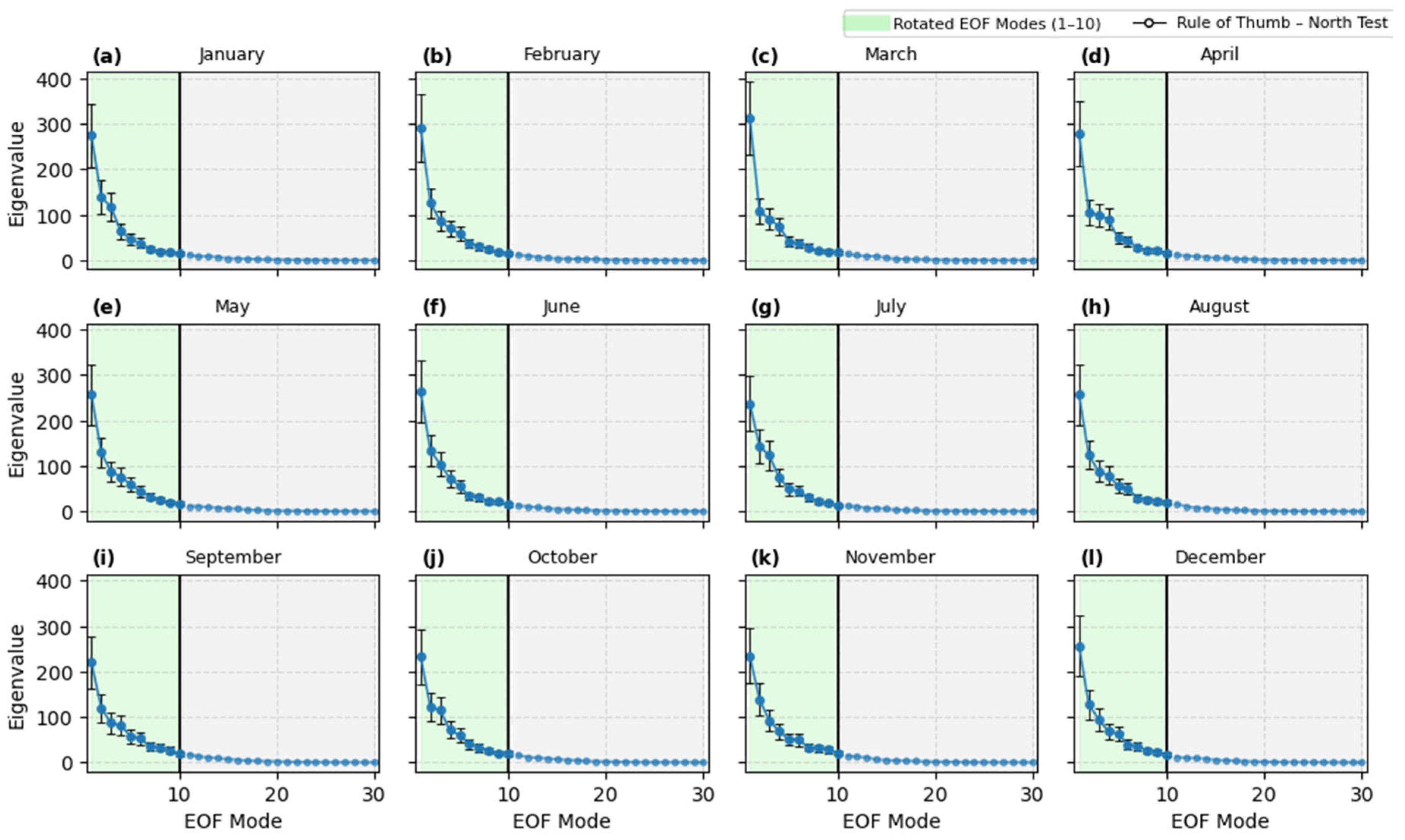
Applying North’s test in our study, the first component (EOF1, which is associated with the SAD) is independent, since its error bar does not overlap that of EOF2 (Figure 2). The other EOFs are predominantly dependents. Because this study also targets the mode resembling the SWSA, we need to maximize the explained variance of modes beyond the first. To do this, we rotate the components obtained from the EOF analysis (explained below). The number of components to rotate must be specified in advance. In this study we are using 10 components. This value was defined through the scree plot (Figure 2), a graphic that shows the eigenvalues by each component. The test scree looks for the point where the slope of the eigenvalue (or explained variance) plot changes abruptly, forming an “elbow” [31]. This point indicates that adding more components does not significantly increase the accumulated explained variance, so it can be stopped there.
Figure 2.
Test scree of each monthly EOF mode (a–l). The black thick line separates the first ten modes that are rotated (green part). The rule-of-thumb North et al. [28] test is displayed as black thin error bar for each of the first 10 modes.
2.2.4. Rotated EOF (REOF)
As the North et al. [28] test indicated a lack of statistical independence among the leading EOF modes (except for EOF1), rotation was applied to redistribute the explained variance and improve the interpretability of the patterns. In this context, modes that are not statistically independent may still represent meaningful climate variability when they exhibit coherent spatial structures and physically consistent relationships with atmospheric circulation.
We used the Varimax rotation [32], an orthogonal technique that redistributes variance among the retained EOFs without changing the total variance explained, with the purpose of enhancing spatial localization and facilitating physical interpretation of the modes [33,34,35]. Accordingly, the Varimax method was applied to the first ten EOF modes, which together explained approximately 91% of the total variance, ranging from 90% in September to 93% in February. Rotation yields new modal variances without altering the total variance obtained with the unrotated EOF solution [36]. Finally, the rotated patterns were examined visually to identify, for each calendar month, the pattern most consistent with the SWSA. This procedure follows the methodology used by Barnston and Livezey [37] to characterize the Pacific–North America (PNA) and North Atlantic Oscillation (NAO) patterns. We would like to emphasize that, although not statistically independent in the strict EOF sense, the SWSA is treated as a climate variability pattern based on its physical coherence, robustness across months, and consistent association with atmospheric circulation and precipitation anomalies over South America, rather than as a mathematical artifact of the rotation.
In Section 3, we do not show plots of the EOF and REOF modes. Instead, we present homogeneous correlation maps, defined as the correlation between the coefficient time series of an EOF or REOF mode obtained with a specific variable and grid-point anomalies of this same variable (e.g., [1,2]). This approach is commonly used because the square of those correlations provides a local measure of the percentage of variance explained by each mode [38]. We also use heterogeneous correlation maps, which are the correlations between a coefficient time series of an EOF or REOF and anomalies of a different variable than the one used to compute the EOF. In both cases, the correlation maps indicate how well the grid-point anomalies of a field can be predicted from the corresponding coefficient time series [2]. Correlation coefficient statistical significance was evaluated using a bilateral Student t-test with 95% confidence [26].
2.3. Simple and Partial Correlation Analysis
To analyze the relationship between South American precipitation and SST variability modes, we computed linear correlation coefficients (), using either simple or partial correlations. Simple correlation refers to the Pearson correlation between two variables. Partial correlation is used when we aim to isolate the influence of a third variable. Mathematically, the partial correlation is computed between two variables, and , while excluding the effects of a third independent variable, (Equation (2)), following Panofsky and Brier [39] and Kayano et al. [8]. In our case, partial correlation is applied to exclude the ENSO effect, (Niño 3.4 SST anomalies) when correlation is computed for the coefficient time series, (SAD or SWSA), and a variable (for instance, mean precipitation anomalies).
where , and are the linear correlations between the coefficient time series and a variable, excluding the effect of variable 2. Here, the correlation coefficient statistical significance was also evaluated using a bilateral Student t-test with 95% confidence [25].
2.4. Composites
While the EOFs/REOFs were computed for the most recent climatological period (1991–2020), we extended the coefficient time series to cover 1980–2025 by projecting monthly SST anomalies onto the EOF (REOF) mode(s) representative of the SAD (SWSA). Therefore, the monthly composites for SAD and SWSA were constructed by averaging the anomaly fields for months in which the mode’s monthly coefficient was above one standard deviation (+1; positive phase) or below one standard deviation (−1; negative phase) computed for the period from 1980 to 2025. Because of the variability from month to month, no fixed threshold was applied; instead, the phase classification was based directly on the monthly standard deviation. For instance, for the SAD in March, the threshold (or ) was ±1.3, while in September, it was ±0.72. All anomalies were defined relative to the 1991–2020 climatological period.
The significance of the observed composites was assessed using a Monte Carlo resampling technique [25], which evaluates whether the anomalies associated with the events are unlikely to occur by random chance. The procedure consists of performing 10,000 random resamplings in which N years (matching the number of event years) are randomly selected without replacement from the original coefficient time series (1980–2025). For each resampling, the mean anomaly field is computed and stored, generating an empirical distribution of composite means for every grid point. From this distribution, the 5th and 95th percentiles are estimated and used as confidence bounds. The observed composite at each grid point is then compared with these thresholds to determine statistical significance. In essence, this method tests whether the mean anomaly observed during the SST mode events (N) is statistically significant when compared to normal year-to-year variability.
3. Results and Discussion
For the SST time series of each calendar month between 1991 and 2020, we computed EOFs. In general, the first three EOF modes together explain approximately 60% of the total variance of each monthly time series, with a maximum in January (65%) and a minimum in September (52%). These values are slightly higher than those (~47%) reported in previous studies [1,2,8]. The following subsections will describe the results for the SAD, represented by the first EOF, and the SWSA, identified through REOF.
3.1. SAD
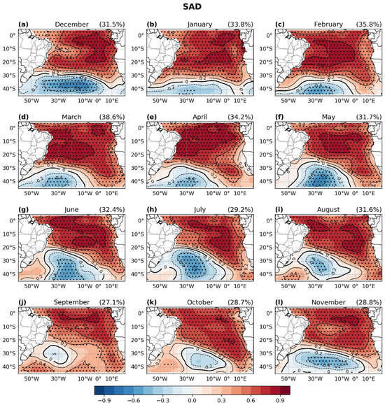
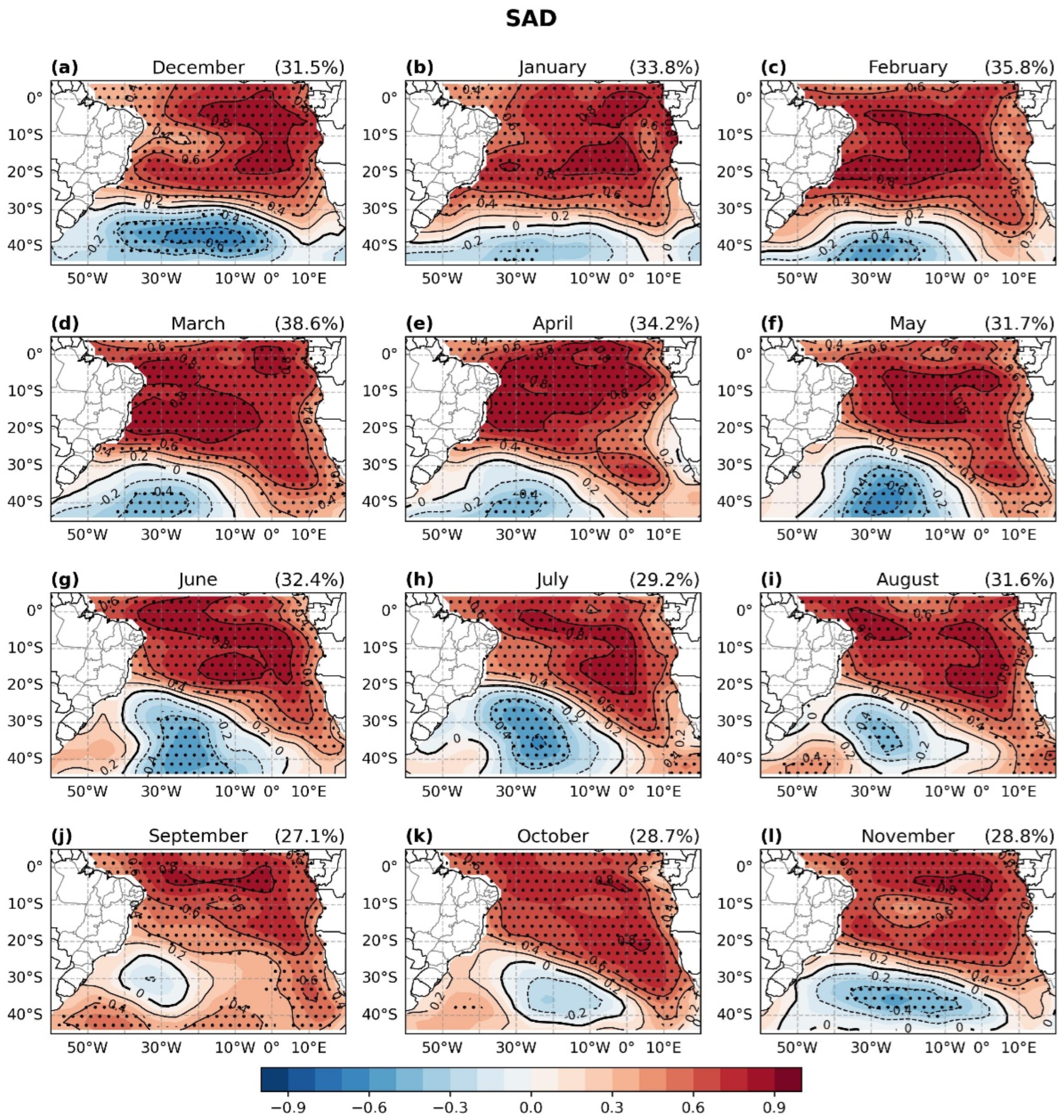
We begin this section by presenting the homogeneous correlation between the EOF1 coefficient time series and the SST anomalies that characterize the SAD, rather than by showing the EOF1 spatial pattern directly (Figure 3). This approach demonstrates the consistency between the mode and the oceanic variable. Most correlations are statistically significant at the 95% level (p< 0.05) (Figure 3, dotted grid points). The coefficient time series of EOF1 for each calendar month is shown in the Supplementary Materials (Figure S1).
Figure 3.
Monthly homogeneous correlation between the EOF1 coefficient time series and SST anomalies (shaded and lines) from January 1991 to December 2020 (a–l). Contour interval: 0.2. Negative contours are indicated in dashed lines, positive contours in thin lines, and the zero contour is thicker. Dotted grid points indicate correlations significant at the 95% level (p < 0.05). Explained variance (%) by the EOF1 for each month is on the top right of the corresponding panel.
The SAD is a physical independent mode (Figure 2) characterized by a northeast–southwest dipolar structure in the SAO, exhibiting a latitudinal gradient near 35° S in the austral summer months (Figure 3a–c) that shifts northward during autumn (Figure 3d–f). Then, the SAD reaches its northernmost position, with the northwest flank near 20° S in the winter months (Figure 3g–i). This variability is linked to the meridional displacement of the systems driven by the apparent sun path. The SAD positive phase is characterized by a dipole with a center of positive SST anomalies in the tropical latitudes and a second one of negative anomalies in the subtropics (Figure 3). Regions with a higher positive correlation (>0.8) migrate throughout the year, from the eastern position in October–January near Africa’s coast (Figure 3k,l,a,b respectively) to the western position in February–April near to Brazil’s coast (Figure 3c–e), being the most affected areas by this mode (see the SAD Composites Section). Independent of the SAD phase, the extratropical core is always smaller than the tropical one, and in early spring (Figure 3i–k) it decays with no significant SST anomalies. The SAD explained variance ranges from 27.1% in September to 38.6% in March. Our findings are consistent with Morioka et al. [5], Nnamchi et al. [4,6], and Kayano et al. [8].
The literature indicates that the growth and decay of the SAD arise from a combination of local atmosphere–ocean interactions and occasional remote forcing, such as from the tropical Pacific. Locally, variations in the SASA, in its strength and meridional position, change the surface wind stress over the SAO. When the anticyclone strengthens or meridionally shifts so that winds are intensified over a region, enhanced wind stress increases evaporation and latent heat loss and deepens the ocean mixed layer. A deeper mixed layer entrains colder subsurface water into the surface layer, producing negative SST anomalies in one pole; simultaneously, weakened winds in the opposite pole produce a shallower mixed layer and reduced heat loss, fostering positive SST anomalies. This chain of wind → mixed-layer change → SST anomaly establishes the opposing SST poles that characterize the SAD [2,5,10,40]. As the system evolves, surface heat flux anomalies and entrainment feedback determine the persistence or decay of the SST poles. Morioka et al. [5] show that the decay phase is dominated by changes in shortwave radiation and diminished vertical mixing, which gradually erase the subsurface temperature contrasts that supported the dipole.
More recently, Santis et al. [41] demonstrated that a “memory effect” can sustain subsurface anomalies below the summer mixed layer, allowing them to re-emerge in subsequent seasons and prolong or reshape the dipole’s life cycle. Together, these studies reveal that the SAD is maintained and terminated by an interplay of atmospheric forcing, mixed-layer adjustment, entrainment processes, and seasonal re-emergence mechanisms. In terms of remote forcings, the PSA wave trains (Rossby waves) propagate into the SAO sector, altering the SASA’s intensity and location and thus preconditioning the local wind and evaporation patterns that set up SAD-like SST contrasts [42].
We also analyzed the heterogeneous correlation between the mean precipitation (mm day−1) and SAD coefficient time series shown in Figure S1. The analysis was then repeated using partial correlations in which the ENSO influence was removed. Both analyses, considering the climatological period from 1991 to 2020, produced very similar spatial patterns and correlation values, indicating that the ENSO has little effect on the SAD (compare Figures S2 and S3), as indicated in Kayano et al. [8] for precipitation. Based on this result, we used the full monthly calendar time series for the composite analysis.
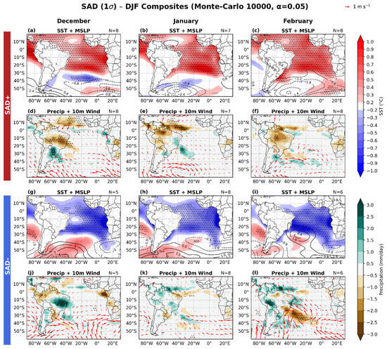
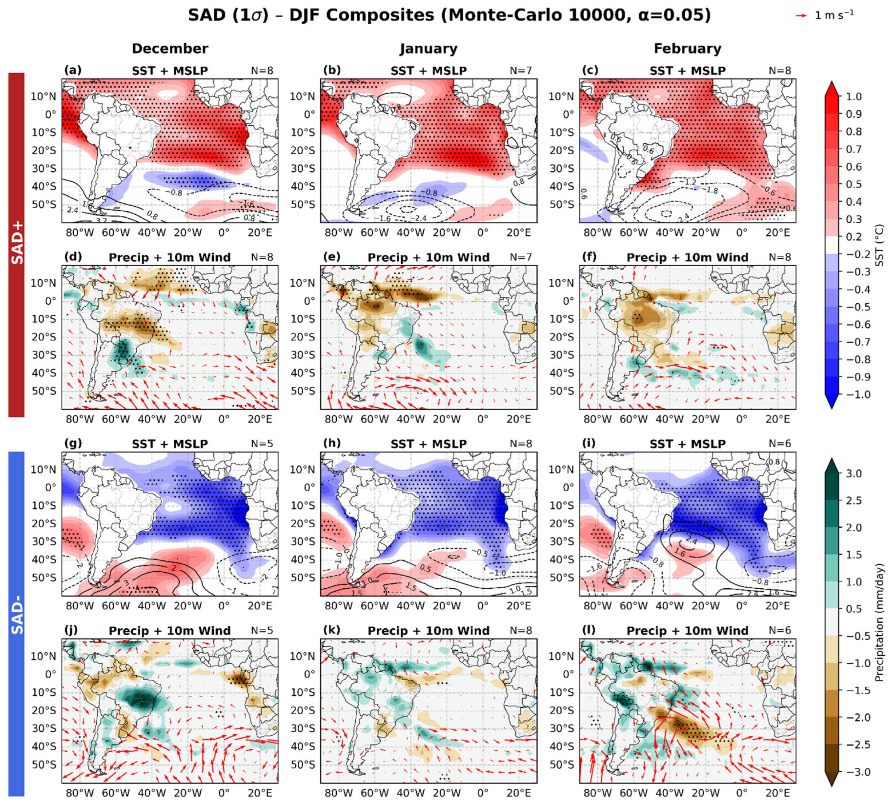
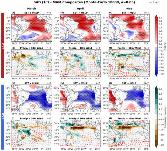
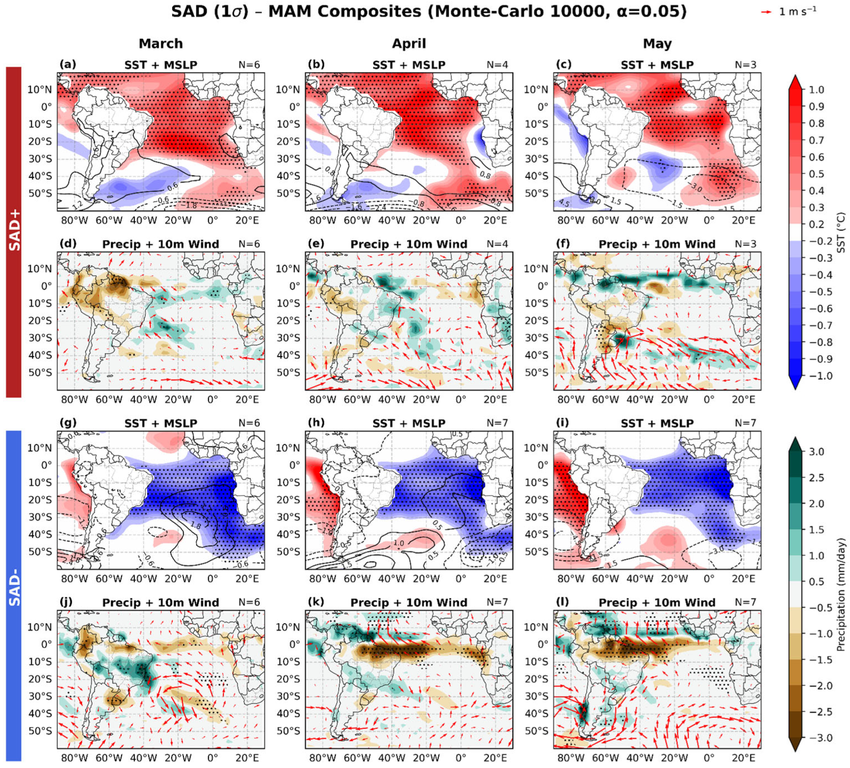
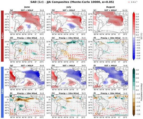
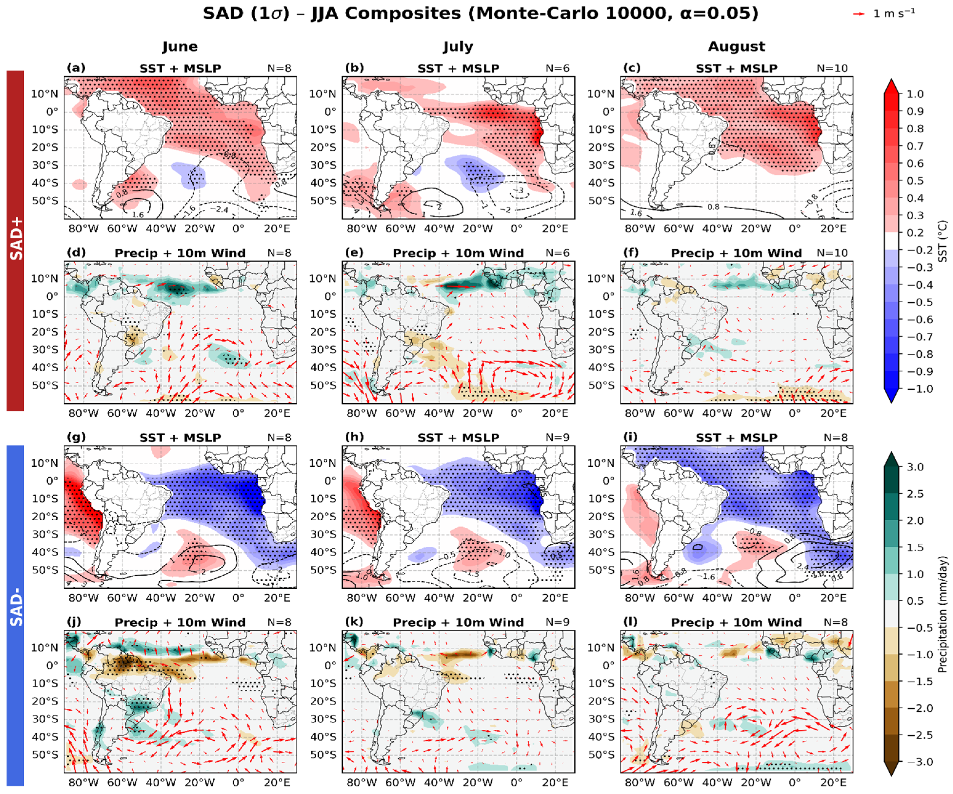
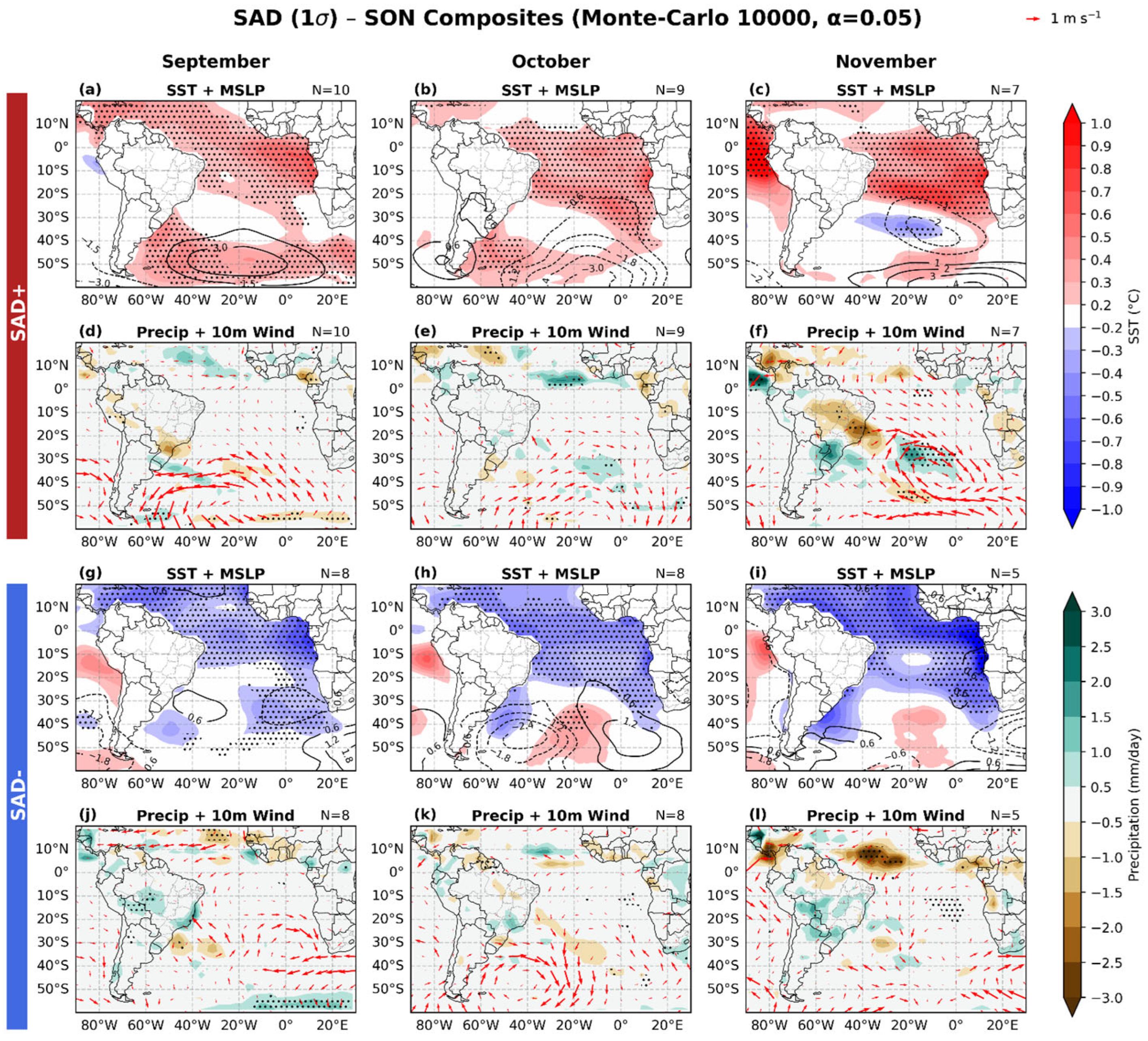
Figure 4, Figure 5, Figure 6 and Figure 7 show the composites for the positive (upper panels, a–f) and negative (lower panels, g–l) phases of the SAD, respectively, SAD+ and SAD−, considering the anomalies of SST, MSLP, precipitation, and 10m wind direction. For the SST and precipitation, a Monte Carlo statistical test was applied using significance at the 95% level (p < 0.05). In most months, the SAD exerts its strongest influence over the ITCZ region, with comparatively weaker effects over subtropical SA rainfall, except during March, May, June, November, and December.
Figure 4.
Composites during the austral summer months (DJF) of (a–c) SST anomalies (°C; shaded in red and blue) with MSLP anomalies (hPa; black contours), and (d–f) precipitation anomalies (mm day−1; shaded in green and brown) and 10m wind vectors (m s−1) for the positive SAD phase; (g–i) and (j–l) are similar to (a–f), respectively, but for the SAD negative phase. Dotted grid points indicate regions where the SST and precipitation anomalies are statistically significant at the 95% confidence level based on a Monte Carlo test. The number of SAD events (N) for each month and phase is shown in the upper-right corner of each panel.
Figure 5.
Similar to Figure 4, but it shows the composites during the austral autumn months (MAM).
Figure 6.
Similar to Figure 4, but it shows the composites during the austral winter months (JJA).
Figure 7.
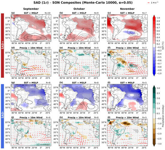
Similar to Figure 4, but it shows the composites during the austral spring months (SON).
We start discussing the composites of the SAD+ phase (Figure 4a–f, Figure 5a–f, Figure 6a–f and Figure 7a–f). During the year, the 10 m wind circulation and MSLP anomalies remain close to the climatological mean, except in the warm core borders, i.e., in the ITCZ region and near 20° S. The SAD+ tends to shift the ITCZ southward, primarily affecting northern SA and producing negative rainfall anomalies in January, February, and March over continental regions such as the Amazon rainforest and the Guianas (Figure 4e,f and Figure 5d). In contrast, as the ITCZ migrates northward in late autumn [43], positive anomalies in April and May become weak and not statistically significant (Figure 5e,f). In addition, the SAD+ phase also impacts the precipitation over the continental and oceanic branches of the SACZ, causing a negative precipitation anomaly observed only in November (Figure 7d) and December (Figure 4d). From November (Figure 7f) to February (Figure 4f), the SAD+ is associated with a wet anomaly over parts of SESA, which is related to an anomalous cyclonic circulation over the south of the domain; however, only in December (Figure 4d) is there a significant signal. It occurs because the winds of the western sector of the anomalous low converge, contributing to the wet conditions. In March and April (Figure 5d,e), this circulation weakens and then reappears in May (Figure 5f). From June to October (Figure 6d–f and Figure 7d), the cyclonic anomaly moves eastward and, near the southern South American coast, an anticyclonic anomaly predominates, except in August (Figure 6f). In this period, few areas exhibit precipitation anomalies over SA.
The most prominent feature of the SAD− phase is its association with a shifted ITCZ northward, which is more evident from March to July, producing negative (positive) anomalies over northern Brazil (Venezuela and Guianas) in the austral autumn and early winter months (Figure 5j,l and Figure 6j,k). The same pattern is observed in January and February (Figure 4k,l), yet with less significance. In part, this appears to be linked to the anomalous southerly winds shown in the region of the ITCZ anomalies. Over SESA, there is no consistent precipitation–anomaly pattern during the SAD− phase, while in the SACZ region, wet anomalies tend to appear in December, January, and March (Figure 4j,k and Figure 5j). In February, the SAD− is associated with anomalous anticyclonic circulation over the warm core near 30° S and cyclonic circulation over extratropical latitudes near Argentina and the Uruguay coast (Figure 4i,l), whereas in June, this pattern is inverted with anomalous cyclonic circulation and wet conditions over SESA (Figure 6g,j).
Much of the precipitation anomaly over SESA is caused by moisture transport via the South American Low-Level Jet (SALLJ) from the tropics to the subtropics [44,45]. As this jet is a characteristic of the 850 hPa level, we also analyzed composites of 850 hPa wind anomalies in the rainy season (see Figure S4). We find that positive precipitation anomalies over SESA during SAD+ coincide with a stronger low-level jet, and negative anomalies during SAD− coincide with a weaker or absent jet, especially in December (Figure S4c,f). However, no consistent cyclonic or anticyclonic circulation pattern appears to control the jet changes between SAD phases.
In summary, our analysis shows a monthly variability in the precipitation anomalies over SA, which could not be identified by Bombardi et al. [7], who evaluated the SAD impact on precipitation in neutral years (without ENSO events) without separating the analyses by months. In their results, in the SAD− (SAD+) phase, the negative (positive) SST anomalies predominate across the Brazilian coast, and in this situation, there are positive (negative) anomalies of precipitation over continental and oceanic branches of the SACZ. We also obtained these results but specifically for December, January, and March (November and December) in the negative (positive) phase. Kayano et al. [8] performed a seasonal analysis of SAD and precipitation only over the continent during the twentieth century and without including circulation anomalies. Most of our results are in agreement with this study, where the SESA and north/northeast Brazil present most of the signal associated with SAD phases.
3.2. SWSA
Since the influence of the SAD on precipitation is more concentrated on the ITCZ rather than SESA, and because Drumond and Ambrizzi [11], consistent with Kayano et al. [8], suggest that an anomalous SST core off the southeastern Brazilian coast can be related to continental rainfall, we searched for an SST mode with a core in the same (or approximately similar) region as indicated by these authors. The oceanic region across the southeast Brazil coast is of particular interest because it is cyclogenetic [46] and hosts the oceanic branch of the SACZ during the rainy season [47]. Figure 2 shows that, except for EOF1, the remaining EOFs are not independent. Therefore, we applied a Varimax rotation to redistribute the variance and to obtain a monthly pattern more similar to the SWSA mode previously identified by Kayano et al. [8]. It is important to note that the lack of independence becomes irrelevant after applying the rotation.
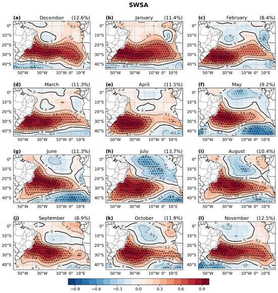
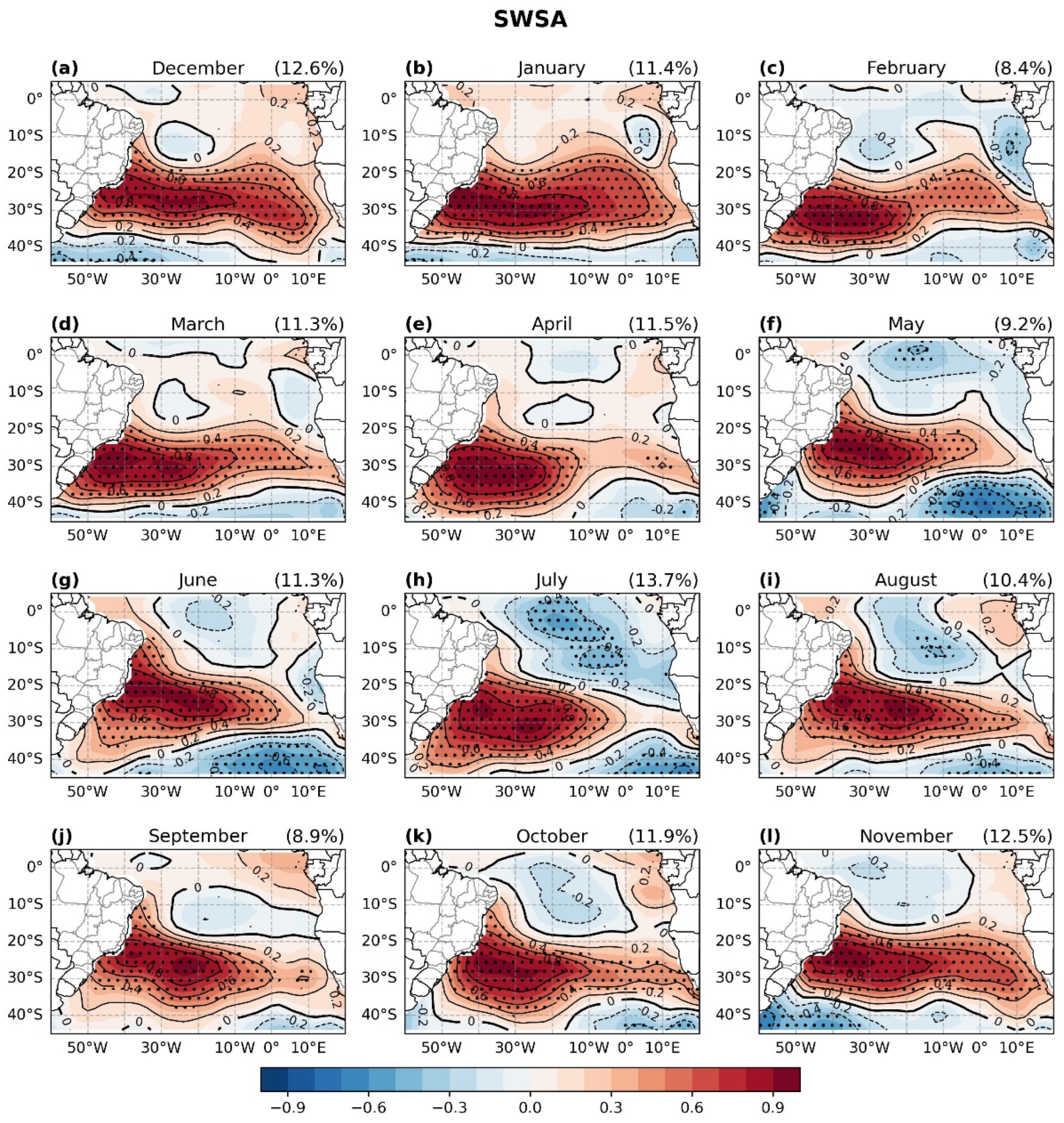
Figure 8 shows the monthly-calendar SWSA patterns obtained with the REOF, while the corresponding coefficient time series are presented in the Supplementary Materials (Figure S5).
Figure 8.
Monthly homogeneous correlation between the rotated SST EOF (REOF), which represents SWSA, and the SST anomalies (shaded and lines) from January 1991 to December 2020 (a–l). Explained variance (%) of each month is on the top right of the corresponding panel. Contour interval: 0.2. Negative contours are indicated in dashed lines, positive contours in thin lines, and the zero contour is thicker. Dotted grid points indicate correlations significant at the 95% level (p < 0.05).
The SWSA mode is characterized by an intense core of SST anomalies extending from the south–southeastern coast of Brazil toward the eastern Atlantic. The core reaches its southernmost position and intensity (near ~30° S) during austral mid-summer and early autumn (Figure 8a–e); by late autumn it migrates northward, expanding along Brazil’s northeast coast. During winter and spring, the core’s maximum oscillates near ~25° S (Figure 8g–l). The SWSA explained variance ranges from 8.4% in February to 13.7% in July.
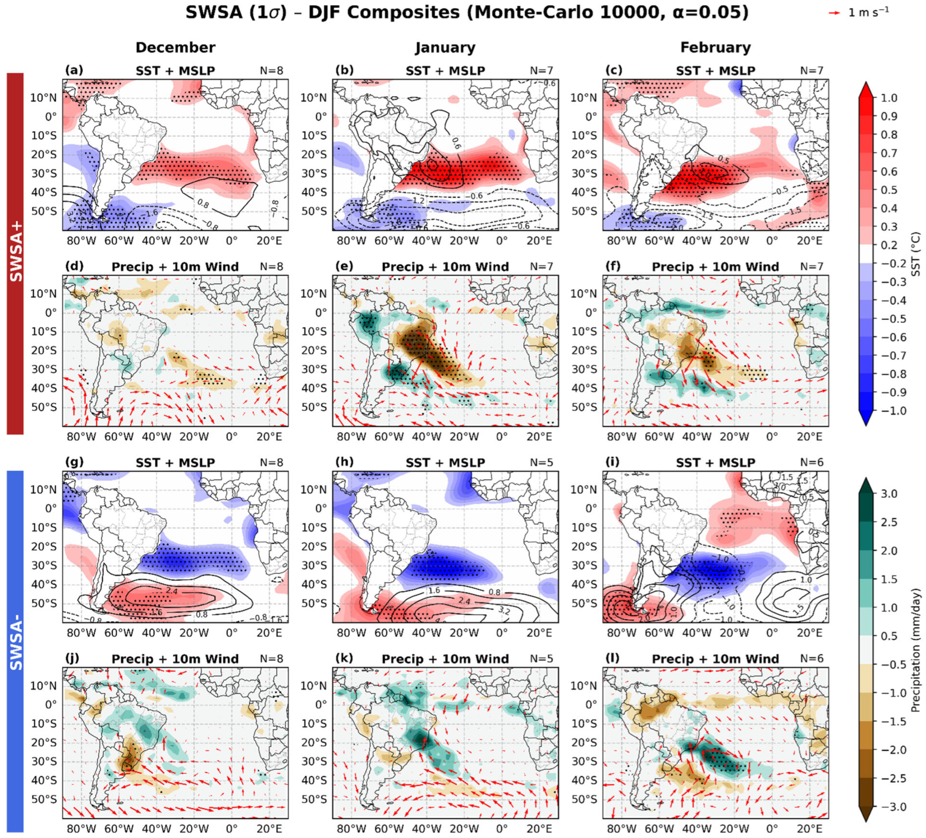
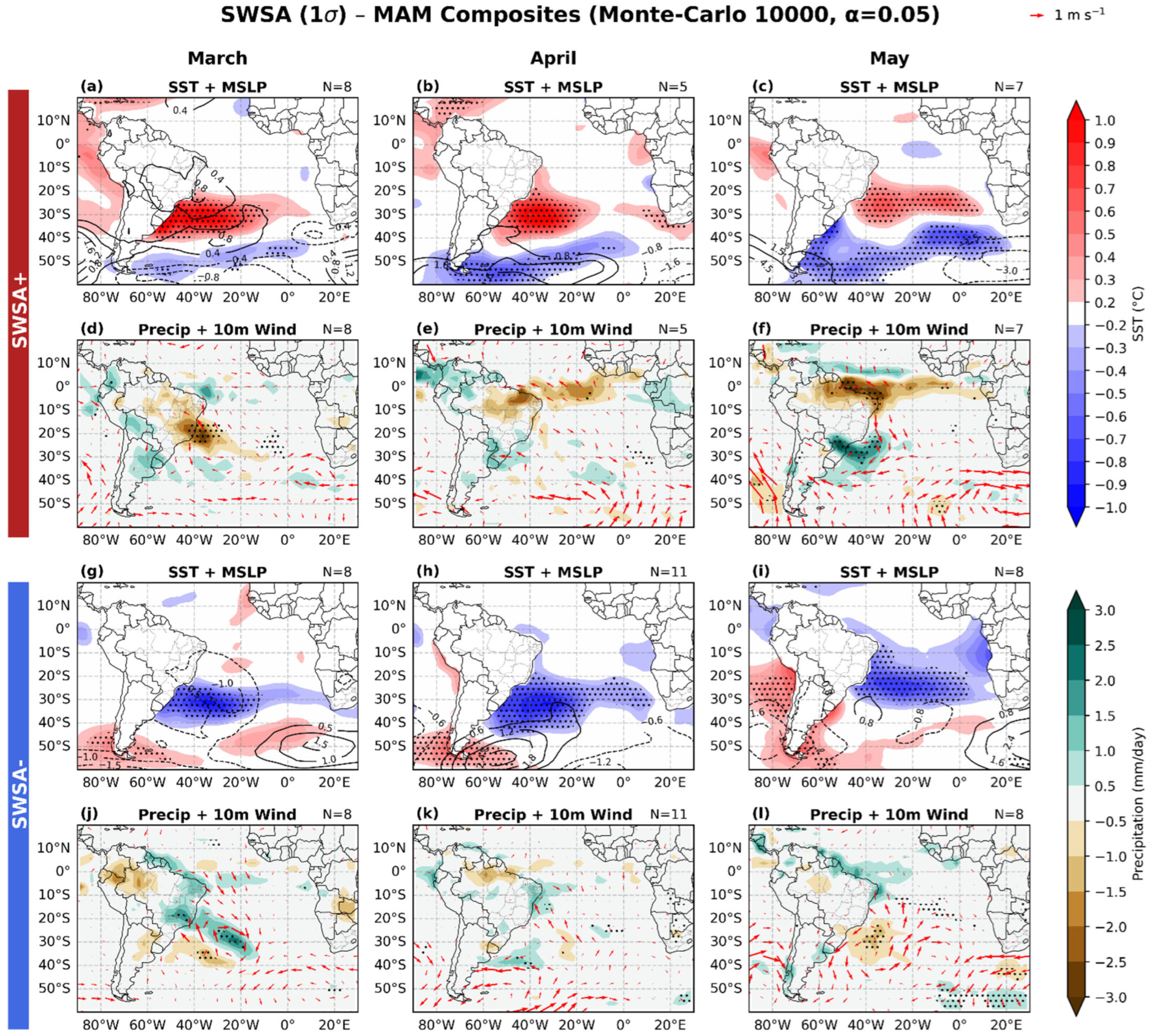
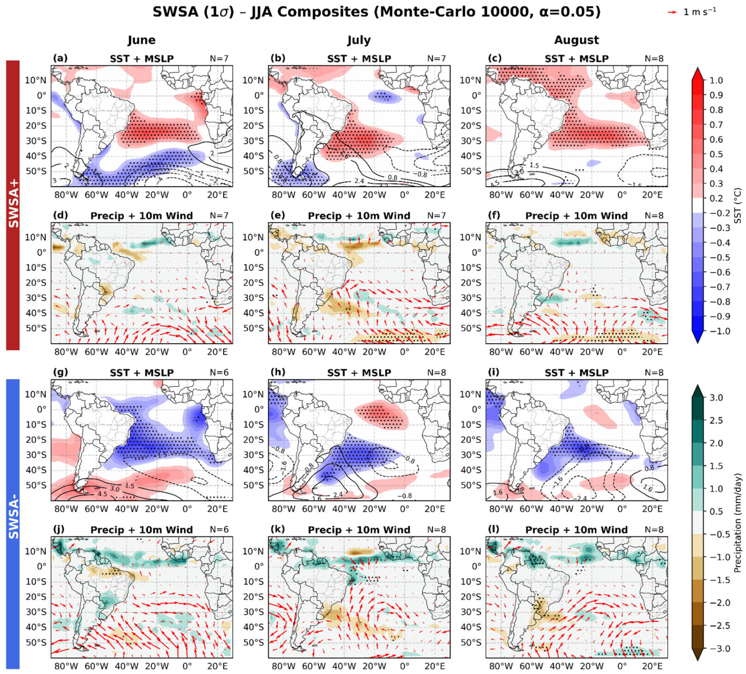
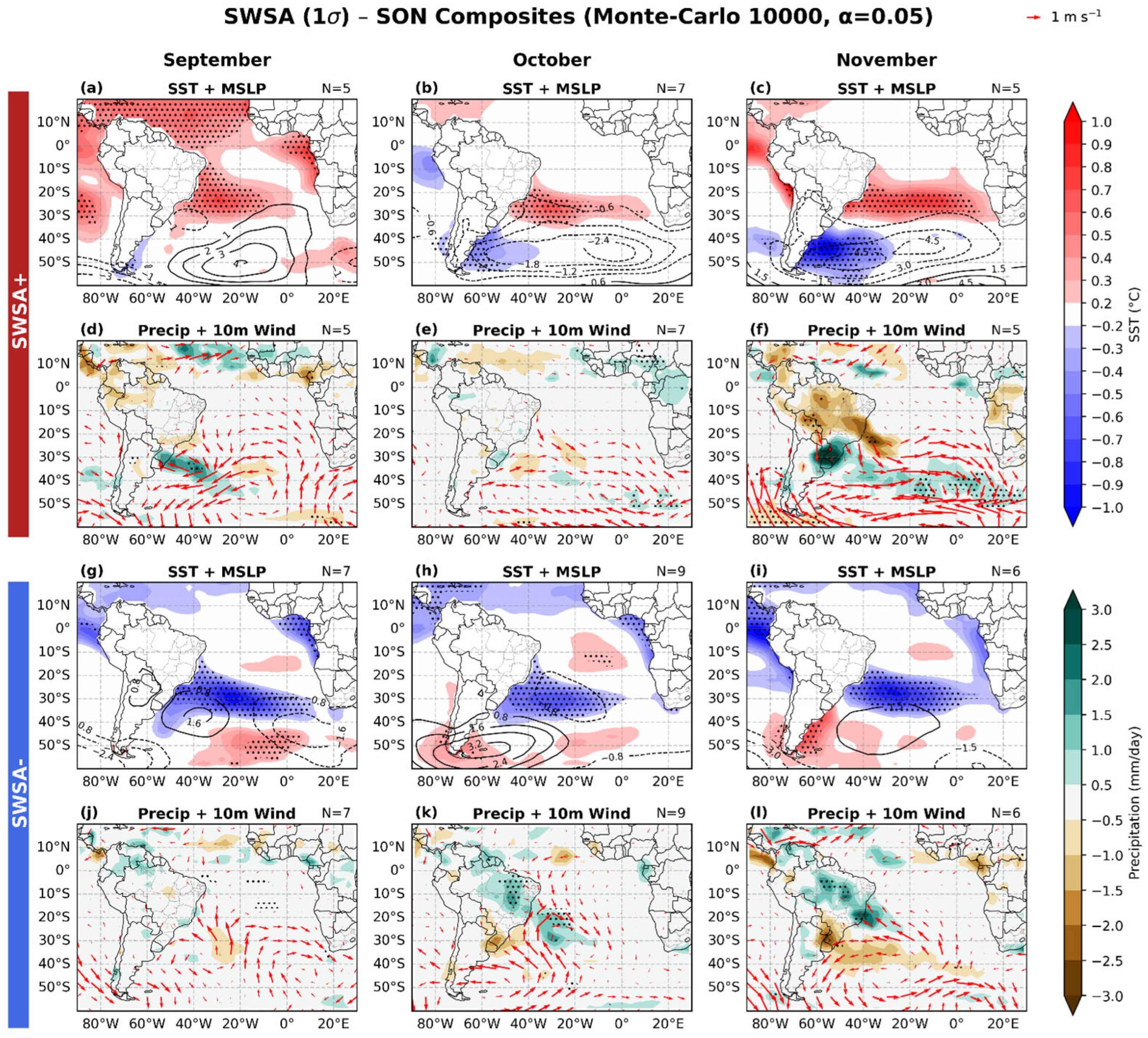
Considering the most recent climatological reference period (1991–2020), the correlations between the EOF coefficient time series and precipitation anomalies, with and without removing the ENSO influence, show only minor differences (cf. Figures S6 and S7). Therefore, we focus on the composite analysis based on the full time series, without excluding ENSO months, consistent with the SAD analysis. Figure 9, Figure 10, Figure 11 and Figure 12 show the composites for the positive (upper panels, a–f) and negative (lower panels, g–l) phases of the SWSA, respectively, SWSA+ and SWSA−, considering the anomalies of SST, MSLP, precipitation, and 10 m wind direction. For the SST and precipitation, a Monte Carlo statistical test was applied using significance at the 95% level (p < 0.05).
Figure 9.
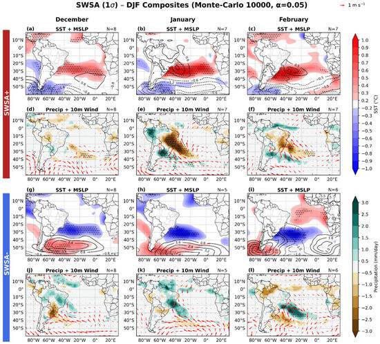
Composites during the austral summer months (DJF) of (a–c) SST anomalies (°C; shaded in red and blue) with MSLP anomalies (hPa; black contours), and (d–f) precipitation anomalies (mm day−1; shaded in green and brown) and 10 m wind vectors (m s−1) for the positive SWSA phase; (g–i) and (j–l) are similar to (a–c) and (d–f), respectively, but for the SWSA negative phase. Dotted grid points indicate regions where the SST and precipitation anomalies are statistically significant at the 95% confidence level based on a Monte Carlo test. The number of SAD events (N) for each month and phase is shown in the upper-right corner of each panel.
Figure 10.
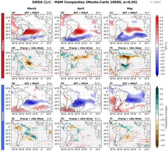
Similar to Figure 9, but it shows the composites during the austral autumn months (MAM).
Figure 11.
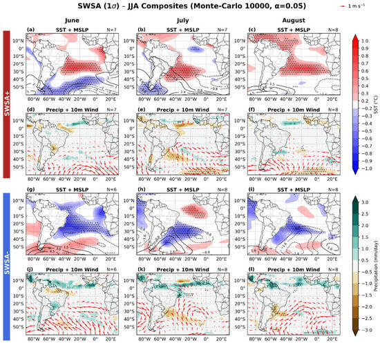
Similar to Figure 9, but it shows the composites during the austral winter months (JJA).
Figure 12.
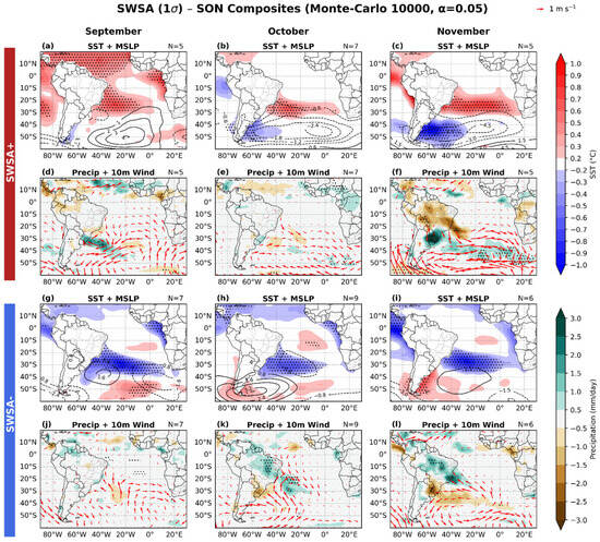
Similar to Figure 9, but it shows the composites during the austral spring months (SON).
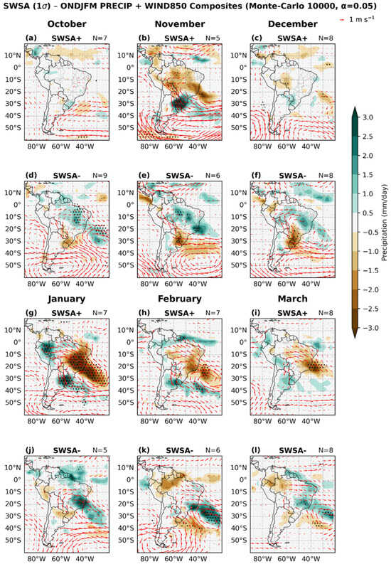
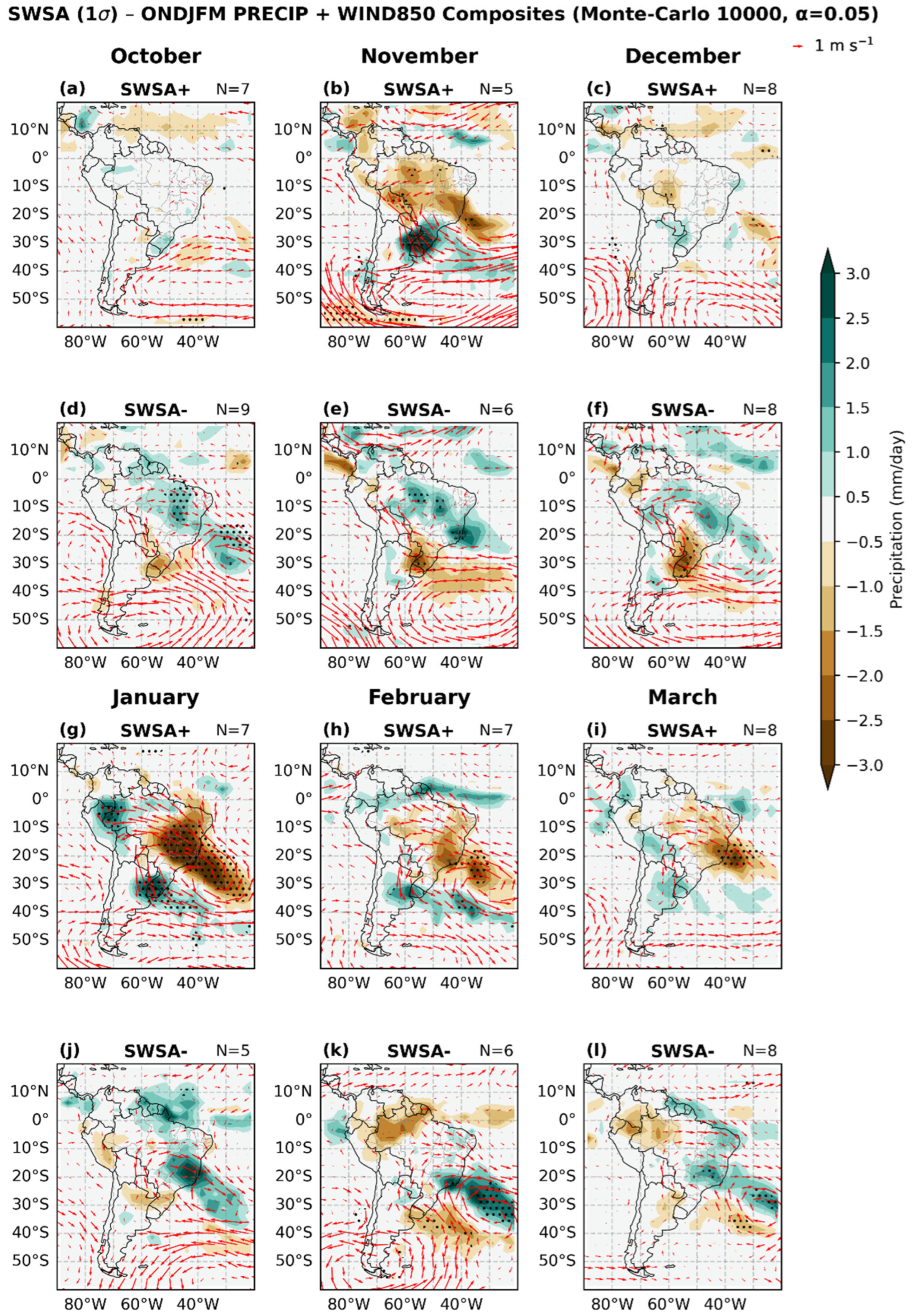
During the SWSA positive phase (SWSA+), positive SST anomalies off southeastern Brazil are linked to negative precipitation anomalies in the region of both continental and oceanic branches of the SACZ from November–March (Figure 9a–f, Figure 10a,d, and Figure 12c,f), except in December (Figure 9d), and are almost absent in the winter and spring seasons (Figure 11a–f and Figure 12a–f). Composites indicate these SST warm anomalies co-occur with positive MSLP in rainy months, meaning anomalous highs allow the ocean to warm while suppressing convection in the SACZ region [48,49,50]. The 10 m wind anomalies also show an anticyclonic circulation associated with reduced precipitation between southeastern Brazil and the SAO (Figure 9e–f, Figure 10d, and Figure 12f). At 850 hPa, the SALLJ is routed from the tropics toward SESA, producing precipitation downstream during the rainy season (Figure 13b,g–i), except in October and December, when this pattern is weaker or absent (Figure 13a,c).
Figure 13.
Composites during the rainy season months (ONDJFM—October to March) of (a–c) and (g–i) precipitation anomalies (mm day−1; shaded in green and brown) and 10m wind vectors (m s−1) for SWSA+; (d–f) and (j–l) are similar but for SWSA−. Dotted grid points indicate regions where precipitation anomalies are statistically significant at the 95% confidence level based on a Monte Carlo test. The number of SWSA events (N) for each month and phase is shown in the upper-right corner of each panel.
Although these patterns resemble El Niño impacts, our partial correlations do not support an El Niño attribution (see Figure S6), so other teleconnection modes may be acting in this monthly timescale. It is important to highlight that the described pattern is consistent with the documented anomalies during two severe droughts in southeastern Brazil: the case of 2001 [11], and the case of 2014 [12]. These authors describe that heat sources in the other ocean basins triggered the Rossby wave trains that contributed to the development of an anomalous high-pressure system over part of southeastern Brazil and the SAO.
The findings of Rodrigues et al. [51] and Artana et al. [52] reinforce this mechanism from a climatological perspective. They demonstrate that tropical convection over the Indian and Pacific Oceans can disturb the atmospheric circulation through Rossby wave propagation. As a result, a strong, barotropic anticyclonic anomaly tends to dominate over part of southeastern Brazil and the adjacent SAO, forming a persistent atmospheric blocking pattern. This circulation not only intensifies drought conditions by suppressing rainfall but also promotes the development of marine heatwaves in the neighboring ocean. According to Rodrigues et al. [50], these marine heatwaves arise from enhanced shortwave radiative warming and reduced ocean heat loss caused by weakened winds under the blocking high-pressure system. Marine heatwaves are prejudicial for the marine systems since they cause fish and coral reef mortality, toxic algal blooms, etc. [53]. In summary, the anomalous atmospheric circulation induced by a Rossby wave train promotes ocean warming and simultaneously suppresses precipitation in southeastern Brazil.
In the SWSA negative phase (SWSA−), cooler coastal SSTs near southeastern Brazil are associated with wetter conditions across the continental and oceanic SACZ region and drier conditions in SESA. This signal is clear from October to March (Figure 9g–l, Figure 10g,j, and Figure 12h,i,k,l). Composites show cyclonic anomalies near the southeastern Brazilian coast, which can strengthen the SALLJ into the SACZ region (the flow goes to the low-pressure area [54]), increasing cloudiness and reducing incoming radiation; a thermodynamic mechanism that explains the cooler SST [13,55]. By contrast, south of this cold core, positive MSLP anomalies predominate and favor a clearer sky and, consequently, radiative SST warming. In addition, the anticyclonic circulation may direct waters from its latitude toward the subtropics; because this water is colder than that in the SACZ region, advection provides an additional dynamic mechanism for cooling the SST [55]. A consequence of the anomalous high pressure is that it prevents the low-level jet from penetrating into SESA and reversing its direction and reinforcing the SACZ region (see Figure 13d–f,j–l).
The cyclonic anomaly near southeastern Brazil induces sea–air heat flux transfer, which helps to channelize the SALLJ and produce cloudiness. These events, following Pezzi et al. [54], are thermodynamic and dynamic mechanisms that act to decrease the SST. The former does this by blocking the radiation decreasing the radiative warming of the sea, and the latter by the cold-water advection by the near-surface anticyclone to the region of the cyclonic anomaly.
To illustrate the SALLJ configuration, an important conduit for moisture transport, Figure 13 shows composites of the precipitation and 850 hPa winds using only months with the strongest precipitation signal. These are the same months used in Fialho et al. [56], who analyzed atmospheric mechanisms associated with SACZ episodes lasting more than seven days. The patterns in our Figure 13 resemble those reported by these authors (notably, our results agree with theirs even though Fialho et al. [56] applied intraseasonal filtering to their data). Fialho et al. [56] link the continental and coastal anomalies to a semi-stationary midlatitude Rossby wave train over the South Pacific with an equivalent-barotropic structure that turns equatorward after crossing the south latitudes of SA; extratropical perturbations favor the tropical–subtropical convection. They interpret oceanic cooling as resulting from coupling between the atmospheric cyclonic circulation and the ocean (e.g., enhanced latent and sensible heat fluxes, upwelling, and surface mixing under cyclonic/wind-anomaly conditions). Increasing cloudiness there is a reduction in the SST radiative warming. Ocean cooling appears to be part of the build-up process that fosters a sustained low-level convergence and moisture transport toward the continent, helping to sustain the SACZ long enough for it to persist for several days.
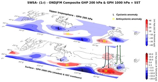
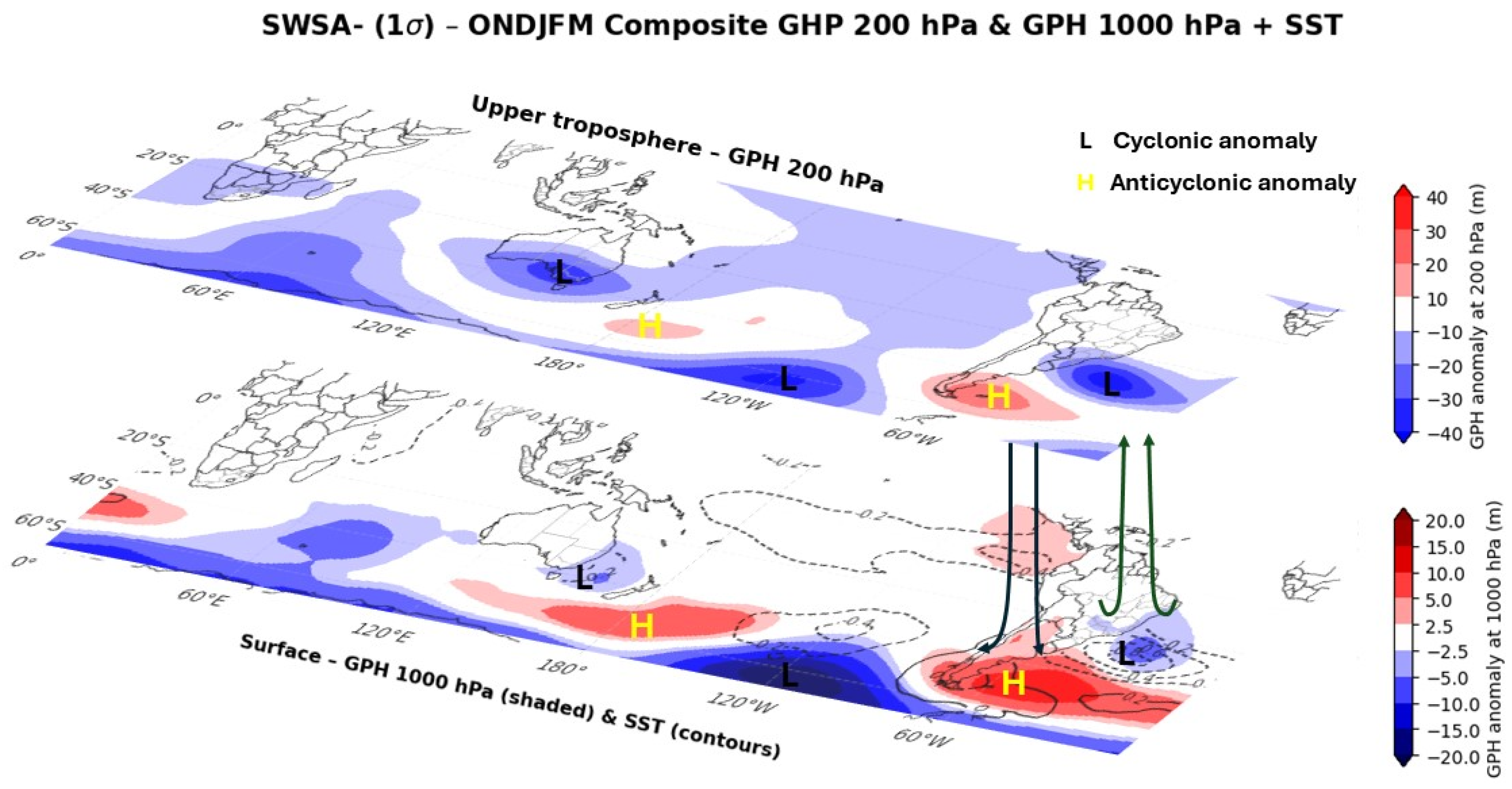
Before discussing the SWSA− phase, note that Figure 14 presents an additional composite analysis of the geopotential height (an indicator of atmospheric circulation) to further explore the physical mechanisms associated with the SWSA mode. We do not intend to identify or redefine the SST patterns discussed previously; rather, this analysis is included to support the physical interpretation of the SWSA mode, particularly in the following discussion of its negative phase. To this end, geopotential height anomalies at 1000 and 200 hPa are analyzed over an expanded domain, allowing the large-scale circulation patterns associated with the SWSA phases to be diagnosed.
Figure 14.
Composite of SST anomalies (°C; contours) and geopotential height anomalies at 1000 and 200 hPa (m; shaded) during the negative phase of the SWSA mode for rainy-season months (ONDJFM; October–March), illustrating the associated large-scale circulation. Composites are constructed using months in which the SWSA REOF time coefficient is lower than −1 standard deviation. Atmospheric fields are derived from ERA5, and anomalies are computed relative to the 1991–2020 climatology.
During SWSA−, cyclonic anomalies over southeastern Brazil and the SAO, together with anticyclonic anomalies farther south, appear to be a response to a Rossby wave train emanating from the Pacific Ocean (Figure 14). This pattern is supported by a composite of 200 and 1000 hPa geopotential height anomalies for the rainy season (ONDJFM) during SWSA−, and it corroborates with the findings of previous studies such as [55]. The mechanisms of the SWSA+ are almost the same, but the Rossby wave produces an anticyclonic anomaly over southeastern Brazil and the SAO, which follows Rodrigues et al. [42,51] and Artana et al. [51].
We also suggest that the SWSA may be connected to the SAM. During the SAM+ phase, negative MSLP anomalies dominate near Antarctica and in subtropical latitudes closer to southeastern Brazil (where a positive cyclone-frequency anomaly is present), while positive anomalies occur around ~45° S (near the Argentine coast). The SAM− phase exhibits the opposite pattern [57,58]. Therefore, the cyclonic (anticyclonic) anomalies along the southeastern Brazilian coast during SWSA− (SWSA+) may be related to the SAM+ (SAM−) phase. In other words, this suggests an inverse correlation between the SAM and SWSA; however, confirming this relationship requires further investigation, including an assessment of the drivers of the SAM, which is beyond the scope of this study.
These results indicate that the precipitation response associated with both the SAD and SWSA is strongly month-dependent. The SAD-related signal is more coherent during the austral summer months, when ITCZ variability dominates, while it weakens or partially reverses during the seasonal migration of the ITCZ. In contrast, the SWSA exhibits a clearer and more physically consistent influence during the rainy-season months (ONDJFM), when its interaction with the SACZ and the SALLJ is strongest. Such features would be partially masked in seasonal or annual analyses.
4. Conclusions
Motivated by the need to revisit SST variability modes in the SAO, this study investigated how South American precipitation responds to different phases of the basin’s leading modes of variability—the SAD, a tropical–subtropical dipole, and the SWSA, a subtropical–extratropical pattern—during the recent climate period (1991–2020). By applying EOF and REOF analyses at the monthly scale, this work addresses the scarcity of month-specific assessments in the literature and provides information that is particularly relevant for subseasonal-to-seasonal (S2S) forecasting. The influence of these modes on precipitation was further evaluated using partial correlation and composite analyses, considering both ENSO-neutral conditions and periods when ENSO events occur. The results indicate that the precipitation responses associated with the SAD and SWSA exhibit a relatively weak dependence on the ENSO, supporting the use of the full monthly dataset in the composite analysis.
The SAD emerges as the dominant SST variability mode in the SAO, consistent with previous studies. It is primarily associated with variations in the strength and meridional position of the SASA [2], which modulate surface wind stress, mixed-layer depth, and air–sea heat fluxes [6]. Although the SAD is identified as an independent mode in the EOF framework, the physical processes governing its persistence and decay remain incompletely understood. In contrast, the SWSA does not appear as a fully independent mode but is more clearly interpreted as an oceanic response to atmospheric forcing, particularly through large-scale circulation anomalies affecting the southwestern and southeastern sectors of the basin.
The precipitation response to the SAD is strongest in tropical latitudes and is closely linked to changes in the position and intensity of the ITCZ. At the monthly scale, the SAD positive (negative) phase is associated with a southward (northward) displacement of the ITCZ during austral summer, leading to dry (wet) conditions over northern SA and wet (dry) anomalies along the northeastern coast of Brazil, particularly between January and March. From April to July, as the ITCZ migrates northward, the precipitation response weakens and partially reverses. Over the SESA and SACZ regions, the SAD-related precipitation signal is generally less spatially organized throughout the year, becoming more evident in specific months, such as December, when SAD+ (SAD−) is associated with reduced (enhanced) precipitation over the SACZ region and opposite anomalies over SESA.
The SWSA mode exhibits its strongest influence during the austral warm season and is more directly associated with variability in the SACZ. During the SWSA positive phase, wetter conditions prevail over SESA, while drier conditions tend to dominate over the continental and oceanic branches of the SACZ. The opposite pattern is observed during the negative phase. This precipitation anomaly pattern is associated with circulation anomalies over the SAO that influence the pathway of the SALLJ. Specifically, cyclonic anomalies near SESA (southeastern Brazil) during the SWSA+ (SWSA−) phase help to channelize the SALLJ to this region, contributing to moisture supply. This relationship is most robust between October and March, highlighting the relevance of the SWSA for intraseasonal modulation of precipitation during the rainy season.
Taken together, these results show that although the impacts of the SAD and SWSA are not uniform throughout the year, the monthly framework adopted here allows the identification of specific calendar months in which the precipitation response is spatially coherent and physically consistent. This framework is intended to complement S2S forecasts by providing physical context, rather than serving as an explicit evaluation of forecast performance. For example, if SST anomalies are forecast for the next one to two months (e.g., March and April) and the model indicates colder (warmer) waters off southeastern (northeastern) Brazil, this configuration resembles the SWSA− (SAD+) phase. In that case, enhanced convection and positive precipitation anomalies may be expected over the SACZ (ITCZ) region.
Future studies should further investigate the physical processes governing the development, persistence, and decay of the SAD and SWSA, with particular emphasis on the relative roles of air–sea coupling, radiative fluxes, mixed-layer dynamics, and large-scale atmospheric circulation. Analyses using high-resolution coupled models and ocean reanalyzes may help clarify the seasonal evolution and phase asymmetries of these modes. Extending the assessment to climate projections would also allow the evaluation of potential changes in the frequency, intensity, and spatial structure of SAO SST variability modes under anthropogenic forcing, with important implications for future precipitation variability over SA.
Supplementary Materials
The following supporting information can be downloaded at https://www.mdpi.com/article/10.3390/jmse14030283/s1: Figure S1: Time series of the monthly SAD index for each calendar month (January–December), shown as black lines. The SAD index was computed by projecting monthly SST anomalies onto the leading EOF mode derived for the most recent climatological period (1991–2020). The resulting coefficient time series was then extended to cover the period 1980–2025 in order to increase the sample size. Red (blue) dashed horizontal lines indicate the positive (negative) monthly thresholds used to identify extreme phases of the SAD. Red (blue) circles mark positives (negatives). Figure S2: Monthly partial heterogeneous correlations between the SAD and mean precipitation anomalies (mm/day) while removing the ENSO effect from January 1991 to December 2020. Contour interval of 0.3, negative contours are dashed and positive contours are thin lines, while shaded grid points indicate correlations significant at the 95% level (p < 0.05) on a bilateral Student t-test. Figure S3: Similar to Figure S2, but with simple correlation. Figure S4: Composites during the rainy season months (ONDJFM) of (a–c) and (g–i) precipitation anomalies (mm day−1; shaded in green and brown) and 10 m wind vectors (m s−1) for SAD+; (d–f) and (j–l) are similar but for SAD−. Dotted grid points indicate regions where precipitation anomalies are statistically significant at the 95% confidence level based on a Monte Carlo test. The number of SAD events (N) for each month and phase is shown in the upper-right corner of each panel. Figure S5: Similar to Figure S1, but for the SWSA obtained with REOF. Figure S6: Similar to Figure S2, but for the SWSA. Figure S7: Similar to Figure S3, but for the SWSA.
Author Contributions
Conceptualization, M.S.R.; methodology, N.C.d.O.N., M.S.R. and A.D.; software, N.C.d.O.N.; validation, N.C.d.O.N., M.S.R. and A.D.; formal analysis, N.C.d.O.N., M.S.R. and A.D.; investigation, N.C.d.O.N.; resources, M.S.R.; writing—original draft preparation, N.C.d.O.N., M.S.R. and A.D.; writing—review and editing, N.C.d.O.N.; visualization, N.C.d.O.N.; supervision, M.S.R.; funding acquisition, M.S.R. All authors have read and agreed to the published version of the manuscript.
Funding
This research was funded by the Conselho Nacional de Desenvolvimento Científico e Tecnológico (CNPq), Fundação de Amparo à Pesquisa do Estado de Minas Gerais (FAPEMIG), Coordenação de Aperfeiçoamento de Pessoal de Nível Superior (CAPES code 001), the Degrees Initiative, and Instituto Tecnológico Vale (R100603.PMP).
Data Availability Statement
The original data presented in the study are openly available in https://climate.copernicus.eu/climate-reanalysis (accessed on 27 March 2025).
Acknowledgments
The authors acknowledge the meteorological centers for providing the datasets used in this study.
Conflicts of Interest
The authors declare no conflicts of interest.
Abbreviations
The following abbreviations are used in this manuscript:
| SST | Sea surface temperature |
| SAO | South Atlantic Ocean |
| SAD | South Atlantic Dipole |
| SAD+ | South Atlantic Dipole positive phase |
| SAD- | South Atlantic Dipole negative phase |
| SWSA | Southwestern South Atlantic |
| SWSA+ | Southwestern South Atlantic positive phase |
| SWSA- | Southwestern South Atlantic negative phase |
| SA | South America |
| S2S | Subseasonal-to-seasonal |
| EOF | Empirical Orthogonal Function |
| REOF | Rotated Empirical Orthogonal Function |
| ERSST | Extended Reconstructed Sea Surface Temperature |
| ENSO | El Niño–Southern Oscillation |
| GPCP | Global Precipitation Climatology Project |
| ITCZ | Intertropical Convergence Zone |
| SACZ | South America Convergence Zone |
| SESA | Southeastern South America |
| PCA | Principal component analysis |
| SVD | Singular value decomposition |
| MSLP | Mean sea level pressure |
| SASD | South Atlantic Subtropical Dipole |
| SASDI | South Atlantic Subtropical Dipole Index |
| SAOD | South Atlantic Ocean Dipole |
| SAODI | South Atlantic Ocean Dipole Index |
| PSA | Pacific–South American |
| SASA | South Atlantic Subtropical Anticyclone |
| SIOD | Subtropical Indian Ocean Dipole |
| GrEC–USP | Climate Studies Group of the University of São Paulo |
| SAM | Southern Annular Mode |
| SAM+ | Southern Annular Mode positive phase |
| SAM- | Southern Annular Mode negative phase |
| NOAA | National Oceanic and Atmospheric Administration |
| CPC | Climate Prediction Center |
| CDS | Climate Data Store |
| PNA | Pacific–North America |
| NAO | North Atlantic Oscillation |
| SALLJ | South American Low-Level Jet |
| DJF | December–January–February |
| MAM | March–April–May |
| JJA | June–July–August |
| SON | September–October–November |
| ONDJFM | October–November–December–January–February–March |
References
- Venegas, S.A.; Mysak, L.A.; Straub, D.N. Evidence for Interannual and Interdecadal Climate Variability in the South Atlantic. Geophys. Res. Lett. 1996, 23, 2673–2676. [Google Scholar] [CrossRef] [Scilit]
- Venegas, S.A.; Mysak, L.A.; Straub, D.N. Atmosphere–Ocean Coupled Variability in the South Atlantic. J. Clim. 1997, 10, 2904–2920. [Google Scholar] [CrossRef] [Scilit]
- Lorenz, E.N. Empirical Orthogonal Functions and Statistical Weather Prediction; Statistical Forecasting Project Rep. 1; MIT Department of Meteorology: Cambridge, MA, USA, 1956; Available online: https://www.scirp.org/reference/referencespapers?referenceid=3268389 (accessed on 16 December 2025).
- Nnamchi, H.C.; Kucharski, F.; Keenlyside, N.S.; Farneti, R. Analogous Seasonal Evolution of the South Atlantic SST Dipole Indices. Atmos. Sci. Lett. 2017, 18, 396–402. [Google Scholar] [CrossRef] [Scilit]
- Morioka, Y.; Tozuka, T.; Yamagata, T. On the Growth and Decay of the Subtropical Dipole Mode in the South Atlantic. J. Clim. 2011, 24, 5538–5554. [Google Scholar] [CrossRef] [Scilit]
- Nnamchi, H.C.; Li, J.; Anyadike, R.N.C. Does a Dipole Mode Really Exist in the South Atlantic Ocean? J. Geophys. Res. 2011, 116, D15104. [Google Scholar] [CrossRef] [Scilit]
- Bombardi, R.J.; Carvalho, L.M.V.; Jones, C.; Reboita, M.S. Precipitation over Eastern South America and the South Atlantic Sea Surface Temperature during Neutral ENSO Periods. Clim. Dyn. 2014, 42, 1553–1568. [Google Scholar] [CrossRef] [Scilit]
- Kayano, M.T.; Andreoli, R.V.; Ferreira De Souza, R.A. Relations between ENSO and the South Atlantic SST Modes and Their Effects on the South American Rainfall. Int. J. Climatol. 2013, 33, 2008–2023. [Google Scholar] [CrossRef] [Scilit]
- Palastanga, V.; Vera, C.S.; Piola, A.R. On the Leading Modes of Sea Surface Temperature Variability in the South Atlantic Ocean. Newsl. Clim. Var. Predict. Programme 2002, 25, 12–15. [Google Scholar]
- Sterl, A.; Hazeleger, W. Coupled Variability and Air-Sea Interaction in the South Atlantic Ocean. Clim. Dyn. 2003, 21, 559–571. [Google Scholar] [CrossRef] [Scilit]
- Drumond, A.R.d.M.; Ambrizzi, T. The Role of SST on the South American Atmospheric Circulation during January, February and March 2001. Clim. Dyn. 2005, 24, 781–791. [Google Scholar] [CrossRef] [Scilit]
- Coelho, C.A.S.; de Oliveira, C.P.; Ambrizzi, T.; Reboita, M.S.; Carpenedo, C.B.; Campos, J.L.P.S.; Tomaziello, A.C.N.; Pampuch, L.A.; Custódio, M.S.; Dutra, L.M.M.; et al. The 2014 Southeast Brazil Austral Summer Drought: Regional Scale Mechanisms and Teleconnections. Clim. Dyn. 2016, 46, 3737–3752. [Google Scholar] [CrossRef] [Scilit]
- Chaves, R.R.; Nobre, P. Interactions between Sea Surface Temperature over the South Atlantic Ocean and the South Atlantic Convergence Zone. Geophys. Res. Lett. 2004, 31, L03204. [Google Scholar] [CrossRef] [Scilit]
- Nnamchi, H.C.; Li, J. Influence of the South Atlantic Ocean Dipole on West African Summer Precipitation. J. Clim. 2011, 24, 1184–1197. [Google Scholar] [CrossRef] [Scilit]
- Barreiro, M. Combined Effects of the Tropical and Extratropical Modes of Variability on Precipitation in Southeastern South America. Oxf. Res. Encycl. Clim. Sci. 2024. [Google Scholar] [CrossRef] [Scilit]
- WMO. Regional Workshop: Translating Advances in ENSO Research to Operations in Latin America and the Caribbean. Available online: https://wmo.int/events/webinar/regional-workshop-translating-advances-enso-research-operations-latin-america-and-caribbean (accessed on 1 January 2025).
- Bier, A.A. Changes in the South Atlantic Dipole and Impacts on the Climate of South America under the Aspect of Climate Change. Ph.D. Thesis, Universidade de São Paulo, São Paulo, Brazil, 2023. [Google Scholar]
- Huang, B.; Thorne, P.W.; Banzon, V.F.; Boyer, T.; Chepurin, G.; Lawrimore, J.H.; Menne, M.J.; Smith, T.M.; Vose, R.S.; Zhang, H.-M. Extended Reconstructed Sea Surface Temperature, Version 5 (ERSSTv5): Upgrades, Validations, and Intercomparisons. J. Clim. 2017, 30, 8179–8205. [Google Scholar] [CrossRef] [Scilit]
- Adler, R.F.; Gu, G.; Sapiano, M.; Wang, J.-J.; Huffman, G.J. Global Precipitation: Means, Variations and Trends During the Satellite Era (1979–2014). Surv. Geophys. 2017, 38, 679–699. [Google Scholar] [CrossRef] [Scilit]
- Hersbach, H.; Bell, B.; Berrisford, P.; Hirahara, S.; Horányi, A.; Muñoz-Sabater, J.; Nicolas, J.; Peubey, C.; Radu, R.; Schepers, D.; et al. The ERA5 Global Reanalysis. Q. J. R. Meteorol. Soc. 2020, 146, 1999–2049. [Google Scholar] [CrossRef] [Scilit]
- Drumond, A.; Nogueira, N.C.O.; Reboita, M.S.; Miguel, G.C. Teleconnection Indices: An Updated Version for the Current Climate. CLIVAR Exchanges No. 84, 2025; pp. 20–25. Available online: https://www.researchgate.net/publication/400028348_Teleconnection_Index_Online_Tool_an_updated_version (accessed on 29 December 2025).
- Chung, C.; Nigam, S. Weighting of Geophysical Data in Principal Component Analysis. J. Geophys. Res. Atmos. 1999, 104, 16925–16928. [Google Scholar] [CrossRef] [Scilit]
- Ramos, A.M.; Lorenzo, M.N.; Gimeno, L. Compatibility between Modes of Low-frequency Variability and Circulation Types: A Case Study of the Northwest Iberian Peninsula. J. Geophys. Res. Atmos. 2010, 115, D0211. [Google Scholar] [CrossRef] [Scilit]
- CPC. NOAA Climate Prediction Center: Teleconnection Pattern Calculation Procedures. Available online: https://www.cpc.ncep.noaa.gov/products/precip/CWlink/daily_ao_index/history/method.shtml (accessed on 19 December 2025).
- Bjornsson, H.; Venegas, S.A. A Manual for EOF and SVD Analyses of Climatic Data; CCGCR (Centre for Climate and Global Change Research): Sydney, Australia, 1997; pp. 112–134. [Google Scholar]
- Wilks, D.S. Statistical Methods in the Atmospheric Sciences; Elsevier: Amsterdam, The Netherlands, 2011; ISBN 978-0-12-751966-1. [Google Scholar]
- Hannachi, A. Patterns Identification and Data Mining in Weather and Climate; Springer Atmospheric Sciences; Springer International Publishing: Cham, Switzerland, 2021; ISBN 978-3-030-67072-6. [Google Scholar]
- North, G.R.; Bell, T.L.; Cahalan, R.F.; Moeng, F.J. Sampling Errors in the Estimation of Empirical Orthogonal Functions. Mon. Weather. Rev. 1982, 110, 699–706. [Google Scholar] [CrossRef] [Scilit]
- Hannachi, A.; Jolliffe, I.T.; Stephenson, D.B. Empirical Orthogonal Functions and Related Techniques in Atmospheric Science: A Review. Int. J. Climatol. 2007, 27, 1119–1152. [Google Scholar] [CrossRef] [Scilit]
- Pais, M.A.; Morozova, A.L.; Schaeffer, N. Variability Modes in Core Flows Inverted from Geomagnetic Field Models. Geophys. J. Int. 2014, 200, 402–420. [Google Scholar] [CrossRef] [Scilit]
- Cattell, R.B. The Scree Test For The Number Of Factors. Multivar. Behav. Res. 1966, 1, 245–276. [Google Scholar] [CrossRef] [Scilit]
- Kaiser, H.F. The Varimax Criterion for Analytic Rotation in Factor Analysis. Psychometrika 1958, 23, 187–200. [Google Scholar] [CrossRef] [Scilit]
- Richman, M.B. Rotation of Principal Components. J. Climatol. 1986, 6, 293–335. [Google Scholar] [CrossRef] [Scilit]
- O’Lenic, E.A.; Livezey, R.E. Practical Considerations in the Use of Rotated Principal Component Analysis (RPCA)in Diagnostic Studies of Upper-Air Height Fields. Mon. Weather. Rev. 1988, 116, 1682–1689. [Google Scholar] [CrossRef] [Scilit]
- Lian, T.; Chen, D. An Evaluation of Rotated EOF Analysis and Its Application to Tropical Pacific SST Variability. J. Clim. 2012, 25, 5361–5373. [Google Scholar] [CrossRef] [Scilit]
- Mestas-Nuñez, A.M. Orthogonality Properties of Rotated Empirical Modes. Int. J. Climatol. 2000, 20, 1509–1516. [Google Scholar] [CrossRef]
- Barnston, A.G.; Livezey, R.E. Classification, Seasonality and Persistence of Low-Frequency Atmospheric Circulation Patterns. Mon. Wea. Rev. 1987, 115, 1083–1126. [Google Scholar] [CrossRef] [Scilit]
- Houghton, R.W.; Tourre, Y.M. Characteristics of Low-Frequency Sea Surface Temperature Fluctuations in the Tropical Atlantic. J. Clim. 1992, 5, 765–772. [Google Scholar] [CrossRef] [Scilit]
- Panofsky, H.A.; Brier, G.W. Some Applications of Statistics to Meteorology; Earth and Mineral Sciences Continuing Education; College of Earth and Mineral Sciences: University Park, PA, USA, 1968; Available online: https://www.scirp.org/reference/referencespapers?referenceid=1990183 (accessed on 19 December 2025).
- Bach, E.; Motesharrei, S.; Kalnay, E.; Ruiz-Barradas, A. Local Atmosphere–Ocean Predictability: Dynamical Origins, Lead Times, and Seasonality. J. Clim. 2019, 32, 7507–7519. [Google Scholar] [CrossRef] [Scilit]
- Santis, W.; Castellanos, P.; Campos, E. Memory Effect of the Southern Atlantic Subtropical Dipole. J. Clim. 2020, 33, 7679–7696. [Google Scholar] [CrossRef] [Scilit]
- Rodrigues, R.R.; Campos, E.J.D.; Haarsma, R. The Impact of ENSO on the South Atlantic Subtropical Dipole Mode. J. Clim. 2015, 28, 2691–2705. [Google Scholar] [CrossRef] [Scilit]
- Nogueira, N.C.d.O.; Machado, P.H.G.; Reboita, M.S.; Reis, A.L. Assessment of the Intertropical Convergence Zone over the Atlantic Ocean through an Algorithm Based on Precipitation. J. Atmos. Sci. Res. 2024, 7, 59–73. [Google Scholar] [CrossRef]
- Montini, T.L.; Jones, C.; Carvalho, L.M.V. The South American Low-Level Jet: A New Climatology, Variability, and Changes. J. Geophys. Res. Atmos. 2019, 124, 1200–1218. [Google Scholar] [CrossRef] [Scilit]
- Reboita, M.S.; Drumond, A.; Ferreira, G.; Zilli, M.T.; Crespo, N.M.; Rodrigues, R.R.; Porfírio da Rocha, R.; Ambrizzi, T. Meteorology and Climate of South America and Surrounding Oceans. In Meteorology and Climate of the Southern Hemisphere; Taschetto, A.S., Ambrizzi, T., Ndarana, T., Eds.; Cambridge University Press: Cambridge, UK, 2025; pp. 284–340. ISBN 978-1-009-35268-0. [Google Scholar]
- Reboita, M.S.; Crespo, N.M.; Rocha, R.P.d.; Gozzo, L.F. Synoptic-Scale Cyclones Affecting South America and the South Atlantic Ocean. In Oxford Research Encyclopedia of Climate Science; Oxford University: Oxford, UK, 2018; ISBN 978-0-19-022862-0. [Google Scholar]
- Carvalho, L.M.V.; Jones, C.; Liebmann, B. The South Atlantic Convergence Zone: Intensity, Form, Persistence, and Relationships with Intraseasonal to Interannual Activity and Extreme Rainfall. J. Clim. 2004, 17, 88–108. [Google Scholar] [CrossRef] [Scilit]
- Nogués-Paegle, J.; Mo, K.C. Alternating Wet and Dry Conditions over South America during Summer. Mon. Wea. Rev. 1997, 125, 279–291. [Google Scholar] [CrossRef] [Scilit]
- Mo, K.C.; Higgins, R.W. The Pacific–South American Modes and Tropical Convection during the Southern Hemisphere Winter. Mon. Wea. Rev. 1998, 126, 1581–1596. [Google Scholar] [CrossRef] [Scilit]
- Nogués-Paegle, J.; Byerle, L.A.; Mo, K.C. Intraseasonal Modulation of South American Summer Precipitation. Mon. Wea. Rev. 2000, 128, 837–850. [Google Scholar] [CrossRef] [Scilit]
- Rodrigues, R.R.; Taschetto, A.S.; Sen Gupta, A.; Foltz, G.R. Common Cause for Severe Droughts in South America and Marine Heatwaves in the South Atlantic. Nat. Geosci. 2019, 12, 620–626. [Google Scholar] [CrossRef] [Scilit]
- Artana, C.; Rodrigues, R.R.; Fevrier, J.; Coll, M. Characteristics and Drivers of Marine Heatwaves in the Western South Atlantic. Commun. Earth Environ. 2024, 5, 555. [Google Scholar] [CrossRef] [Scilit]
- Rodríguez-Fonseca, B.; Calvo-Miguélez, E.; Montoya-Carramolino, L.; Rodrigues, R.R.; Polo, I.; Martín-Rey, M.; Losada, T.; López-Parages, J.; Gómara, I.; Rivas, D.; et al. ENSO Impacts on Marine Ecosystems and Fisheries in the Tropical and South Atlantic. Nat. Rev. Earth Environ. 2025, 7, 43–59. [Google Scholar] [CrossRef] [Scilit]
- Campetella, C.M.; Vera, C.S. The Influence of the Andes Mountains on the South American Low-Level Flow. Geophys. Res. Lett. 2002, 29, 7-1–7-4. [Google Scholar] [CrossRef] [Scilit]
- Pezzi, L.P.; Quadro, M.F.L.; Lorenzzetti, J.A.; Miller, A.J.; Rosa, E.B.; Lima, L.N.; Sutil, U.A. The Effect of Oceanic South Atlantic Convergence Zone Episodes on Regional SST Anomalies: The Roles of Heat Fluxes and Upper-Ocean Dynamics. Clim. Dyn. 2022, 59, 2041–2065. [Google Scholar] [CrossRef] [Scilit]
- Fialho, W.M.B.; Carvalho, L.M.V.; Gan, M.A.; Veiga, S.F. Mechanisms Controlling Persistent South Atlantic Convergence Zone Events on Intraseasonal Timescales. Theor. Appl. Climatol. 2023, 152, 75–96. [Google Scholar] [CrossRef] [Scilit]
- Reboita, M.S.; da Rocha, R.P.; Ambrizzi, T.; Gouveia, C.D. Trend and Teleconnection Patterns in the Climatology of Extratropical Cyclones over the Southern Hemisphere. Clim. Dyn. 2015, 45, 1929–1944. [Google Scholar] [CrossRef] [Scilit]
- Reboita, M.S.; Ambrizzi, T.; Crespo, N.M.; Dutra, L.M.M.; Ferreira, G.W.D.S.; Rehbein, A.; Drumond, A.; Da Rocha, R.P.; Souza, C.A.D. Impacts of Teleconnection Patterns on South America Climate. Ann. N. Y. Acad. Sci. 2021, 1504, 116–153. [Google Scholar] [CrossRef] [Scilit]
Disclaimer/Publisher’s Note: The statements, opinions and data contained in all publications are solely those of the individual author(s) and contributor(s) and not of MDPI and/or the editor(s). MDPI and/or the editor(s) disclaim responsibility for any injury to people or property resulting from any ideas, methods, instructions or products referred to in the content. |
© 2026 by the authors. Licensee MDPI, Basel, Switzerland. This article is an open access article distributed under the terms and conditions of the Creative Commons Attribution (CC BY) license.