


Abstract
Route planning for the Northeast Passage must balance transportation costs against navigational risks arising from changing sea ice conditions. Route-wide navigability assessment under adverse scenarios requires explicit representation of sea ice forecast uncertainty. This study proposes a multi-objective route-planning method integrating seven-day sea ice forecasts, paired scenario construction, path-level conditional value-at-risk (CVaR) assessment, and receding-horizon planning. Sea ice scenarios are constructed from seven-day forecasts produced by a convolutional long short-term memory (ConvLSTM) model and historical paired residuals. A* search generates candidate routes using weighted edge costs based on voyage time, propulsion fuel consumption, and cumulative ice-condition severity, the time integral of a local severity score over sailing and waiting. For each scenario, the loss counts each edge of the remaining route once if it is unnavigable at any time within the seven-day forecast window. The CVaR of this loss is included as the fourth objective in Pareto nondominated filtering and fixed-scale scoring to select the route for execution. Model predictive control (MPC) replans over a seven-day horizon and executes for up to 24 h from the updated vessel position and cumulative execution state. In the 2024 evaluation, day-7 root mean square errors (RMSEs) for sea ice concentration and thickness were 24.23% and 22.87% lower, respectively, than those of the persistence baseline. The expanded evaluation compares four strategies in 64 simulations across 16 departure dates in 2024 using one parameterized Arc6-class Aframax tanker. The static strategy completes all 16 voyages; each of the three dynamic strategies completes 15. Across the 15 departure dates with completed voyages under all four strategies, the proposed strategy reduces mean cumulative ice-condition severity by 0.379 score·h relative to the dynamic three-objective strategy, with mean increases of 0.138 h in voyage time and 0.598 t in propulsion fuel consumption. The framework converts forecast uncertainty into path-level window CVaR for decisions on transportation cost, ice-condition severity, and forecast-window navigability risk.
1. Introduction
An Arctic route that is feasible at departure may still be obstructed by sea ice when the vessel reaches the relevant waters [1]. Changing ice and weather conditions affect attainable vessel speed and the probability of a ship becoming beset in ice [2]. For the Northeast Passage, which serves transport demand between Asia and Europe, route planning affects navigation efficiency and fuel costs, vessel safety, and polar environmental protection. Spatiotemporal variations in sea ice concentration and thickness create interdependencies among navigability, attainable vessel speed, and consumption during a voyage [3,4]. Forecast errors further complicate route selection in advance [5]. Integrating sea ice forecasting, risk analysis, and shipping optimization is, therefore, an important research direction for supporting dynamic decision-making in the Northeast Passage.
Route planning in ice-covered waters translates environmental conditions and vessel performance into navigability constraints and route costs. Lehtola et al. [3] integrated sea ice, bathymetry, and ship–ice interactions to estimate attainable vessel speeds and support A*-based route search. Complementary numerical and experimental studies further relate ice conditions to vessel performance through model-scale ice modeling [6], reviews of ship–ice interaction simulation methods [7], viscoelastic ice-plate deformation under dynamic loading [8], and ship resistance experiments in managed ice floe fields [9]. Liu et al. [10] formulated voyage time, fuel consumption, and navigational risk as route-planning objectives, used improved A* to generate routes under different weight combinations, and applied Lifelong Planning A* (LPA*) for dynamic updates.
To accommodate temporal changes in sea ice, research on dynamic route planning has further introduced environmental updates and route replanning mechanisms. LPA*-based multi-objective planning adjusts routes using daily environmental information [10]; an improved D* Lite method reduces repeated search following environmental changes through local updates [11]; and RouteView incorporates sea ice and meteorological factors, including ice floes, sea fog, and sea spray icing, into online route planning so that decisions can be adjusted as navigational conditions change [1,12]. Environmental updates record how ice conditions change between decision times. Forecast-error scenarios describe several possible future ice fields at one decision time.
The development of sea ice forecasting systems such as neXtSIM-F [13], together with the public release of the NOAA/NSIDC Sea Ice Index, Version 4 [14], and ERA5 data [15], has provided methodological and data foundations for Arctic sea ice forecasting and route planning. The datasets actually used in this study and their respective purposes are described in Section 2.2. Spatiotemporal deep learning provides data-driven approaches to short-term sea ice forecasting. Liu et al. [16] used a convolutional long short-term memory (ConvLSTM) model for daily prediction of Arctic sea ice concentration, learning spatial patterns and their temporal evolution from sequences of sea ice data. Point forecasts give a single future ice field. Path-level risk assessment also requires accounting for the dependence of forecast errors across locations, sea ice variables, and lead times.
Research on Arctic navigation risk encompasses accident probabilities, accident evolution, and uncertainty in transportation performance. Methods such as Bayesian networks integrate environmental, vessel-related, and human factors to assess navigational accident risks and the risk of ships becoming beset in ice [17,18], while studies based on resilience theory examine functional coupling at different stages of an accident and approaches to risk control [19]. In route optimization, Sibul et al. [5] combined expected voyage time with the conditional value-at-risk (CVaR) of voyage time, allowing transportation performance under adverse ice conditions to inform route selection.
Cumulative ice-condition severity, as defined in this study, is the time integral, over sailing and waiting, of a local ice-condition severity score determined by sea ice concentration and thickness. CVaR is the tail mean of a scenario loss distribution [20]. Under seven-day sea ice scenarios, navigability restrictions on multiple edges of the remaining route form a path-level loss. Including path-level window CVaR in route selection can change the selected route and its predicted voyage time, propulsion fuel consumption, and cumulative ice-condition severity. Realized voyage outcomes depend on the executed route segments, encountered ice conditions, and subsequent replanning. Forecast errors at different locations, in different sea ice variables, and at different lead times act jointly on route navigability. A single forecast field, or separate treatment of errors by location and variable, leaves out this joint structure [21]. Voyage time, fuel consumption, and cumulative ice-condition severity add over edges. Path-level window CVaR is calculated by summing edge failure indicators within each scenario and then evaluating the CVaR of the resulting route loss. With the route, scenario ensemble, and confidence level held fixed, summed edge-level window CVaR is an upper bound on path-level window CVaR [20]. In receding-horizon planning, only the first part of the current plan is executed before the route is replanned from the updated state [22]. The evaluation, therefore, examines both same-state route selection and full-voyage performance.
The framework integrates seven-day sea ice forecasts, paired scenario construction, path-level CVaR assessment, and receding-horizon planning for the Northeast Passage. Paired scenarios are constructed from ConvLSTM forecasts and historical forecast residuals, preserving the correspondence among sea ice concentration, thickness, spatial locations, and forecast lead times so that dependent forecast errors enter the risk assessment of an entire route. Candidate routes are generated from voyage time, propulsion fuel consumption, and cumulative ice-condition severity, and the path-level CVaR of seven-day navigability failures along the remaining route is included in nondominated filtering and composite scoring. Receding-horizon execution uses a seven-day planning horizon and an execution horizon of up to 24 h, carrying forward the vessel’s actual position and cumulative execution state at each step. Same-state comparisons and complete voyages separate the effect of receding-horizon updates from the effect of the CVaR objective.
The remainder of this paper is organized as follows. Section 2 describes the study area and publicly available datasets, and Section 3 presents the methodological framework. Section 4 reports the case study results. Section 5 discusses the implications and limitations, and Section 6 concludes the paper.
2. Study Area and Data Fusion
2.1. Study Area and Grid
The study domain covers the Northeast Passage from to and from to . It is discretized into a regular latitude–longitude grid with a grid size of . The north–south spacing between adjacent nodes is approximately 27.8 km, whereas the east–west spacing varies with latitude; edge lengths are calculated as great-circle distances from node coordinates. Land and bathymetric information are obtained from the GEBCO 2026 terrain dataset [23] and mapped onto the route grid using nearest-neighbor sampling. Within the area covered by valid sea ice data, land is identified from terrain elevation, and the minimum navigable water depth is set to 1.15 times the design draft, namely 16.1 m. Land cells, cells with missing terrain data, and cells with insufficient water depth are excluded to construct a static geometric navigability mask. Connections between adjacent grid cells follow the navigability and diagonal-movement criteria specified in Section 3.3.1. The representative case-study route connects the Bering Strait (, ) and Murmansk (, ).
Figure 1a shows the study area, route grid, and major marginal seas, with a green triangle and a red star marking the origin and destination, respectively. Figure 1b presents an enlarged view of the boxed region, where gray grid cells indicate those excluded by the static geometric screening. Figure 1c further illustrates the connections between the central grid cell and its eight neighboring cells. All panels use a common color scale, with shades of blue representing the mean September sea ice concentration over 2014–2023; darker shades indicate a higher fraction of sea ice coverage.
Figure 1.
Study area of the Northeast Passage (a), route grid (b), and eight-neighbor connectivity (c). The green triangle and red star mark the origin (Bering Strait) and destination (Murmansk), respectively.
2.2. Public Data Sources
Table 1 summarizes the public datasets from multiple sources integrated in this study.
Table 1.
Public datasets from multiple sources integrated in this study.
Sea ice concentration and thickness are obtained from the daily mean dataset within the CMEMS Arctic Ocean Sea Ice Reanalysis product [24]. Following temporal matching, coordinate harmonization, and grid conversion, the CMEMS, ERA5, and NSIDC data are aligned to a regular grid spanning – and –. CMEMS sea ice concentration and thickness are mapped onto the target grid using bilinear interpolation; for target points lying no more than outside the range of source grid centers, the nearest source boundary values are used. ERA5 data have the same resolution as the target grid and are aligned directly by coordinates. The arithmetic mean of values at 00:00, 06:00, 12:00, and 18:00 UTC each day is used as the daily meteorological input. NSIDC sea ice concentration is mapped using nearest-neighbor sampling to avoid mixing coastline, land, and missing-data codes during interpolation. NSIDC data are used for sea ice concentration validation and M4S correction, whereas preprocessed CMEMS data are used for sea ice thickness. Monthly mean sea ice data for 2014–2023 are used to analyze the climatological background. In the dynamic route experiments, future sea ice inputs are generated by the frozen seven-day forecasting model described in Section 3.1 and Appendix A, and scenario ensembles are constructed from the corresponding historical residuals. Daily CMEMS reference fields, comprising M4S-corrected sea ice concentration and uncorrected sea ice thickness, provide the current initial sea ice conditions and the environment for execution replay.
2.3. Construction of Sea Ice Forecasting Samples and Data Partitioning
In this study, CMEMS sea ice concentration is corrected using isotonic regression [26], combined with monthly fitting and constraints on ice-covered areas; this correction is denoted M4S. The corrected concentration and uncorrected CMEMS sea ice thickness are jointly used as prediction targets. Using the NSIDC product as a reference, a monotonic nondecreasing mapping weighted by the cosine of latitude is fitted for each month using quality-controlled paired samples from 2019–2021. The fitted parameters are then fixed and used to apply a consistent transformation to data from all years. The corrected values are constrained to . Grid cells with an original concentration of zero remain at zero, whereas those with an original concentration of at least 15% retain a corrected concentration of at least 15%. The model has eight input channels: corrected sea ice concentration, sea ice thickness, and the ERA5 variables of 10 m zonal wind, 10 m meridional wind, 2 m air temperature, 2 m dewpoint temperature, low cloud cover, and total cloud cover. All variables are matched by date and grid cell on the grid. The data cover 15 June to 7 November in each year from 2019 to 2024, yielding 876 common dates. Each sample uses seven consecutive days of historical information as input, and neither the input sequence nor the prediction target sequence spans multiple calendar years.
Data from 2019–2021 are used for model training and for fitting normalization and M4S parameters, while data from 2022 are used for model selection. After the model is frozen, data from 2023 are used for historical residual construction and scenario calibration, and data from 2024 are used for prediction performance evaluation and route replay.
3. Methods
Figure 2 presents the methodological framework. First, ConvLSTM generates seven-day sea ice point forecasts, which are combined with calibrated historical residuals to construct paired scenarios. Subject to navigability constraints, voyage time, propulsion fuel consumption, and cumulative ice-condition severity are calculated from the point forecasts, and candidate routes are generated using A* searches with multiple weight combinations. The point-forecast costs of each candidate route are then calculated, and the paired scenarios are used to calculate the CVaR of the entire remaining route over the seven-day window. Pareto filtering and fixed-scale scoring determine the route to be executed. Each execution period lasts no more than 24 h. The actual vessel position and cumulative execution state are then updated before the next planning cycle, forming the dashed feedback loop in the figure. RRI diagnostics, LPA* consistency checks, and B-spline smoothing and continuous execution interface validation are shown separately at the bottom of the figure, apart from the main planning loop.
Figure 2.
Overall framework for multi-objective route planning in the Northeast Passage under sea ice forecast uncertainty.
3.1. Seven-Day Sea Ice Forecasting and Paired Scenario Construction
A seven-day direct multi-lead forecasting model is developed using ConvLSTM [27]. The model takes an eight-channel environmental sequence spanning seven consecutive days as input and simultaneously predicts sea ice concentration and thickness for forecast days 1–7. After training, the model parameters are fixed, and the same model is used to construct historical residuals and support route planning. The network architecture and training settings are provided in Appendix A. The main symbols and their meanings are listed in Appendix B.
Paired scenarios are constructed from the historical forecast residuals of the frozen seven-day forecasting model in 2023. Let denote the kth historical forecast initialization date, the forecast lead time, i the grid cell, and v either sea ice concentration or thickness. The corresponding residual is
where y denotes the reference sea ice field and the model point forecast. Each source date corresponds to one residual member containing both variables, all spatial grid cells, and all seven lead times. The route experiments for 2024 consistently use source members from 2023.
Sea ice scenarios are constructed through state-dependent scale calibration and historical residual rank pairing, with the latter drawing on the idea of reordering based on historical sample ranks [28]. Scale calibration adjusts residual magnitudes according to the current forecast ice conditions. Rank pairing preserves the correspondence of each historical source member across grid cells, variables, and forecast lead times, allowing the residuals at different locations to jointly form a complete sea ice scenario. For decision time t, forecast lead time ℓ, and grid cell i, a state feature vector is constructed from the point forecasts of sea ice concentration and thickness and their local spatial differences:
where C and H are the point forecasts of sea ice concentration and thickness, respectively. Concentration is expressed as a fraction between 0 and 1, and thickness is entered in meters. The quantities and are the mean absolute differences in concentration and thickness, respectively, between the central grid cell and its valid ocean cells in the four-neighbor neighborhood; they are set to zero when no valid neighbors are available.
The scale functions are fitted to the forecast residuals from 2023, separately for each forecast lead time and sea ice variable. Fitting samples are taken from ocean cells with forecast concentration of at least 0.15. Each valid calibration date receives equal weight, and grid cells within a date are weighted by their areas. The regression basis consists of an intercept, the four state features, the squared terms of the first two features, and their interaction. All basis functions except the intercept are standardized using the weighted means and standard deviations of the calibration samples; the resulting design vector is denoted by . Using as the response variable, the coefficients are estimated by ridge regression [29]. The fitting objective combines the weighted mean squared error with the sum of squared non-intercept coefficients, with a regularization coefficient of 0.01. The values of are for concentration and for thickness, with thickness residuals expressed in meters. The resulting state-dependent residual scale is
where restricts x to the interval , and and are the minimum and maximum fitted log-scales among the calibration samples, respectively. Historical residuals are divided by their corresponding fitted scales and pooled using the same date and area weights to establish an empirical quantile mapping for the standardized residuals. At each grid cell, variable, and lead time, the rank position of each historical residual member is calculated and combined with the scale corresponding to the current state. The calibrated residual at decision time t is, therefore,
For each grid cell, sea ice variable, and forecast lead time, the rank position is determined from the ordering of the 2023 historical residuals among the members:
where is the residual rank of member k, with average ranks assigned to tied residuals. The member index k associated with the same historical source date is retained across all grid cells, variables, and lead times. Residuals at different locations and for different variables, thus, form sea ice scenarios through their common member identity, providing consistent inputs for accumulating losses along the entire route within each scenario.
The applicability of state calibration is determined by historical forecast states. First, the four-dimensional state features are standardized using the weighted means and standard deviations of the 2023 calibration samples, with a lower bound of on the standard deviation. Within the predicted ice-covered region of each valid source date, systematic sampling based on cumulative grid-area weights then selects up to 256 grid-cell states as support samples for that date. A current forecast state must satisfy two conditions: each feature must lie within the corresponding range of the historical calibration samples, and at least 20 distinct source dates must each contain a support sample within a standardized Euclidean distance of 2.0 from that state. States satisfying these conditions are considered to have historical sample support.
Scale calibration is applied only to grid cells and variables with forecast concentration of at least 0.15, historical state support, and nonconstant local member residuals. If the range of member residuals for a given grid cell, variable, and lead time does not exceed , the residuals are treated as constant. The original historical residuals are retained outside the predicted ice-covered region, when historical state support is absent, or when local residuals are constant. If fewer than 20 valid fitting dates are available, state calibration is disabled for that lead time. The scale functions, empirical quantile mappings, and state-support information are all established using the 2023 data and remain fixed during subsequent scenario generation.
Combining concentration and thickness into a sea ice state vector, the scenario fields are obtained by adding calibrated residuals to the current point forecasts:
where restricts concentration to and thickness to nonnegative values. If either variable is zero, both are set to zero to ensure consistency of the ice-free state. The current sea ice analysis used as the initial condition is shared by all members and, together with the scenarios for the following seven days, forms a 168 h evaluation window. All candidate routes at a given decision time use this same scenario ensemble, allowing their losses and path-level CVaR values to be compared under the same possible ice conditions. Figure 3 illustrates the point forecasting, residual calibration, rank pairing, and scenario construction procedures. Solid lines indicate computational dependencies, and dashed lines indicate inputs from the historical residual archive.
Figure 3.
Seven-day sea ice forecasting and paired scenario construction.
3.2. Vessel Navigability Constraints and Voyage Costs
This section defines vessel navigability constraints and the costs associated with voyage time, propulsion fuel consumption, and cumulative ice-condition severity. Under a fixed sea ice field, the three costs are accumulated over route segments for candidate search. Dynamic route selection and execution replay use forecast fields and reference fields, respectively, with consistent rules for advancing the vessel position and calculating costs.
3.2.1. Vessel Model and Navigability Constraints
An Arc6-class Aframax tanker representative of summer and autumn energy transport through the Northeast Passage is selected as the study vessel. The vessel has a length between perpendiculars of m, a molded breadth of m, a design draft of m, and a shaft power of 17,000 kW [10]. Its design speed in open water is 12 kn. The minimum navigable water depth is set to 1.15 times the design draft, or 16.1 m.
Equivalent ice thickness is used to represent the combined effects of sea ice concentration and thickness:
where and denote sea ice concentration and thickness in grid cell i, respectively, and is the equivalent ice thickness in that cell. A truncated speed model based on the Parabolic Icebreaking Curve Model (PICM) [30] is then used to calculate the attainable vessel speed under different ice conditions:
where denotes relative shaft power. The coefficients are
For a segment connecting adjacent navigable grid cells, the arithmetic mean of the speeds at the two endpoints is used as the mean segment speed:
The PICM model parameters are listed in Table 2.
Table 2.
Parameters of the PICM continuous speed model.
3.2.2. Voyage Time
Under a fixed sea ice field, the great-circle segment length is calculated using the Haversine formula. Together with the mean segment speed , it gives the segment voyage time and the voyage time of the entire route:
where is in kilometers, in knots, and in hours. These equations are used for candidate route search and evaluation under a fixed sea ice field.
During dynamic forecast evaluation and voyage execution replay, the attainable speed is updated as ice conditions along the route change, and the vessel advances with a continuously represented position. If the next segment is temporarily unnavigable while the current position remains navigable, the vessel waits in place. The dynamically accumulated voyage time comprises sailing time and waiting time:
where is the time during which the vessel is actually moving, and is the time spent waiting in place because of navigability restrictions. In the full-voyage results, voyage time is the cumulative elapsed time from departure to arrival or voyage termination. For dynamic route selection, the voyage time of the entire remaining route comprises sailing and waiting time within the forecast window plus a terminal voyage-time estimate for the remaining distance beyond the window, as detailed in Section 3.4.1.
3.2.3. Ice-Condition Severity Score and Cumulative Ice-Condition Severity
A local ice-condition severity score is constructed from sea ice concentration and thickness. Integrating this score over time during both sailing and waiting yields cumulative ice-condition severity, which serves as the third route-planning objective.
Let and denote sea ice concentration and thickness in grid cell i, respectively. Based on the risk index values for the Arc6 ice class in Table 1 of Reference [31], thickness intervals with identical coefficients are merged, and the coefficient for all m is set to . The resulting piecewise coefficient is
where sea ice thickness is expressed in meters. The ice-condition severity score of grid cell i is defined as
The ice-condition severity score is dimensionless and ranges from 0 to 1. With other conditions unchanged, the score does not decrease as sea ice concentration increases or the thickness category rises. It quantifies the severity of local ice conditions, whereas grid-cell navigability is determined by the specified navigability constraints. Under a fixed sea ice field, the cumulative ice-condition severity of segment is calculated as the mean score of its two endpoint cells multiplied by the segment voyage time:
During dynamic forecast evaluation and voyage execution replay, cumulative ice-condition severity is calculated from the continuous vessel position and time-varying ice conditions. Computational intervals along the grid polyline are divided at grid-cell boundaries, and the nearest grid cell to the current vessel position determines the local ice-condition severity score. Concentration and thickness are linearly interpolated in time between consecutive daily sea ice fields, with piecewise integration when thickness crosses a category threshold. Cumulative ice-condition severity during the dynamic process is expressed as
where s denotes time and is the nearest grid cell assigned to the vessel’s continuous position at time s under a common grid-assignment rule. Here, and denote the sets of sailing and waiting times, respectively. During sailing, the local ice-condition severity score changes with both vessel position and ice conditions. During waiting, the vessel position remains fixed, but the local score can still change with local ice conditions. The score is integrated over time in both cases; waiting, therefore, contributes to both cumulative voyage time and cumulative ice-condition severity. With time measured in hours, cumulative ice-condition severity is expressed in and is not restricted to .
3.2.4. Propulsion Fuel Consumption
The total resistance of a vessel operating in ice consists of calm-water resistance and ice resistance. Calm-water resistance is calculated using the Holtrop–Mennen method, including frictional resistance and the hull-form contribution, appendage resistance, wave-making resistance, additional bulbous-bow resistance, immersed-transom resistance, and model–ship correlation resistance [32]. Ice resistance is calculated using the hybrid model developed by Ryan et al.: the empirical ice-floe resistance equation proposed by Huang et al. is used when equivalent ice thickness does not exceed 0.30 m, whereas an equivalent-ice-thickness resistance relationship based on the Finnish–Swedish ice class rules is used above 0.30 m [4,33]. Total resistance and calm-water resistance are expressed as
where , , and denote total, calm-water, and ice resistance, respectively; is frictional resistance; is the hull-form factor; is appendage resistance; is wave-making resistance; is additional bulbous-bow resistance; is immersed-transom resistance; and is model–ship correlation resistance. Because detailed geometric parameters are unavailable, the relevant bulbous-bow, immersed-transom, and appendage areas are idealized in the baseline model. Based on total resistance, vessel speed, and propulsion-system efficiencies, effective power, delivered power, and brake power are calculated as
where , , and denote effective, delivered, and brake power, respectively. The efficiencies , , , and are the hull, propeller open-water, relative rotative, and shaft-transmission efficiencies, respectively. Resistance in kilonewtons and speed in meters per second yield power in kilowatts. The baseline values are , , , and . The main-engine specific fuel oil consumption (SFOC) is 168 .
The nodal fuel consumption rate, segment fuel consumption, and total fuel consumption of the entire route are expressed as
where is in ; and denote auxiliary power and auxiliary specific fuel oil consumption, respectively; is the fuel consumption of segment ; is its voyage time; and is the total fuel consumption of route P. Baseline fuel consumption accounts for the main propulsion system, with . The effect of auxiliary loads is examined through sensitivity analysis.
If the delivered power required at the PICM speed in a grid cell exceeds the 17 MW shaft-power limit, the power requirement at 2 kn is checked first. If it still exceeds the limit, the cell is classified as unnavigable. Otherwise, 36 bisection iterations are performed between 2 kn and the PICM speed, and the final feasible lower bound is used as the attainable speed in that cell.
The segment fuel equations above are used for candidate search under a fixed sea ice field. During dynamic forecast evaluation and voyage execution replay, the attainable speed satisfying the power constraint and the fuel consumption rate are updated according to the ice conditions in the grid cell corresponding to the continuous vessel position. Propulsion fuel consumption is accumulated over sailing time:
where follows the grid-assignment definition in Section 3.2.3, and is the main-propulsion fuel consumption rate in the corresponding grid cell at time s, in . The rate is approximated piecewise linearly and integrated over time intervals delimited by changes in ice conditions and navigability events.
The waiting-fuel sensitivity analysis calculates adjusted fuel consumption as for each recorded execution trajectory. Here, is a prescribed combined fuel consumption rate for auxiliary engines and station keeping during waiting, and is cumulative waiting time in hours. The tested rates are . Fuel rankings are compared among completed voyages with the same departure date.
3.2.5. Fixed Reference Scales and Three-Objective Segment Costs
Fixed reference scales are used to nondimensionalize the three segment costs so that voyage time, propulsion fuel consumption, and cumulative ice-condition severity can be evaluated jointly:
where , , and are the voyage time, propulsion fuel consumption, and cumulative ice-condition severity of segment , respectively, and the overbar denotes a nondimensionalized quantity. The reference scales are h, t, and . They remain fixed across candidate-generation steps so that identical cost differences have consistent nondimensional representations. For candidate-generation weights , the composite segment cost is defined as
The composite route cost is obtained by summing the segment costs along the route, namely . The weights and reference scales jointly determine the relative contributions of the costs, and varying the weights generates candidate routes with different objective preferences. Path-level CVaR is calculated after complete candidate routes have been generated and is subsequently considered together with the three voyage costs in route selection.
3.3. Candidate Route Generation and Path-Level CVaR Evaluation
3.3.1. Candidate Route Generation Using Scalarized Segment Costs
The study waters are represented as a directed graph , where V is the set of navigable grid nodes and E is the set of segments connecting adjacent navigable nodes. Eight-neighbor connectivity is used: each grid cell is connected to at most four orthogonal and four diagonal neighboring cells.
Within the coverage of valid environmental data, a static geometric navigability mask is first constructed from land and water-depth information, excluding land cells and cells shallower than 16.1 m. The set of navigable nodes V is then determined from the sea ice state in each forecast snapshot using the ice-condition and power constraints specified in Section 3.2.1 and Section 3.2.4. For a diagonal connection, both endpoints and the two corresponding orthogonal neighboring cells must satisfy the navigability conditions. If any of these cells is unnavigable, the diagonal segment is not constructed, preventing routes from cutting across the corners of obstacle cells. These node-screening and adjacency rules jointly define the feasible search graph for each forecast snapshot.
On the feasible graph constructed for each forecast snapshot, A* [34] searches using the composite segment cost defined in Section 3.2.5. For source node s, destination node d, and current node n, the accumulated search cost, heuristic, and node evaluation function are defined as
where is the currently recorded path from the source to node n during the search; is the great-circle distance from the node to the destination, in kilometers; kn is the maximum vessel speed; and is the voyage-time reference scale.
The heuristic is the weighted normalized time cost of reaching the destination along the shortest great-circle distance at the maximum vessel speed. Because the actual remaining path is no shorter than this distance, attainable speed does not exceed , and propulsion fuel consumption and cumulative ice-condition severity are nonnegative, the heuristic is admissible and consistent. A*, therefore, finds the route with the minimum composite cost for the corresponding forecast snapshot and weight combination.
When , the heuristic vanishes, and Dijkstra’s algorithm [35] is used. For , a lexicographic rule is applied in the order of cumulative ice-condition severity, voyage time, and propulsion fuel consumption. Cumulative ice-condition severity is minimized first; ties are resolved by comparing voyage time and then propulsion fuel consumption.
To examine the basic trade-off between voyage time and fuel consumption, the two-objective baseline comparison under a fixed sea ice field uses 21 weight combinations, as specified in Section 4.3. Forecast-driven route planning jointly considers voyage time, propulsion fuel consumption, and cumulative ice-condition severity, using the following seven three-objective weight combinations to generate candidate routes:
The three components of each weight vector correspond, in order, to voyage time, propulsion fuel consumption, and cumulative ice-condition severity. Their values are
At each decision driven by the seven-day forecast, feasible graphs and segment costs are constructed separately for the L1–L7 point-forecast snapshots. Searches with the seven weight combinations are performed on each snapshot, yielding 49 search combinations. The resulting routes are pooled with the unexecuted portion of the previous route, and duplicate route geometries are removed to obtain the current candidate set:
where is the number of candidates after deduplication, which varies with forecast ice conditions, actual vessel position, and route overlap.
When the vessel is inside a directed edge, every new candidate first retains the remaining portion of that edge and then searches for the subsequent route from its forward endpoint, preventing replanning from changing the actual vessel position.
3.3.2. Seven-Day Window Failure Loss and Path-Level CVaR
All candidate routes use the same ensemble of 133 paired sea ice scenarios. The number of edges experiencing navigability failure within the window is first accumulated separately for each scenario, and path-level CVaR is then calculated. At decision time t, let be a candidate remaining route and h the forecast-window length. For scenario k and segment e, let denote the set of grid cells involved in the navigability check. This set includes the two endpoint cells and, for a diagonal segment, the two orthogonal neighboring cells used to prevent corner cutting through obstacles. At decision time t, let denote the navigability state of cell i at future time under scenario k, taking a value of 1 when the specified navigability conditions are met and 0 otherwise. The window failure indicator for segment e is defined as
This indicator uses the entire forecast window as the assessment interval. It equals 1 if any relevant grid cell experiences navigability failure at any time within the window and 0 otherwise. The navigability conditions are the same as those used in route planning and voyage execution, including static geometric, equivalent-ice-thickness, and propulsion-power constraints. Statically unnavigable regions are excluded before candidate generation. Sea ice concentration and thickness are interpolated in time between the current analysis and daily forecast anchors, and changes in navigability are checked. Under scenario k, the window loss of the candidate remaining route is
Each edge of the candidate remaining route is counted once if it becomes unnavigable at any time within the seven-day window, independently of estimated vessel arrival times. This common assessment window supports route-wide screening for potential navigability restrictions. The resulting loss and CVaR are expressed in failed-edge units. Execution-failure probabilities require a separate evaluation of navigability along time-resolved vessel trajectories. Route geometry and grid segmentation affect the failed-edge count, so comparisons use the same grid, adjacency rules, and navigability criteria. If the vessel is inside a directed edge, its unexecuted portion participates in the window evaluation as one edge of the current remaining route.
For K equally weighted scenarios, the expected window loss and the proportion of scenarios with at least one edge experiencing window failure are, respectively,
where is the proportion of window failure events in the current scenario ensemble. Following the CVaR minimization representation of Rockafellar and Uryasev [20], path-level window CVaR at confidence level is defined as
where is the seven-day window failure loss of candidate remaining route under scenario k at decision time t; is an auxiliary loss-threshold variable; and . CVaR is measured in failed-edge units and is calculated as the weighted mean over the worst 5% of scenario probability mass. Because , the tail includes the six scenarios with the largest losses and part of the probability mass of the boundary scenario, with the latter equal to . Figure 4 illustrates this calculation: the step curve is the empirical quantile function of the window failure loss, the vertical dashed line marks the 95% quantile boundary, and the two horizontal dashed lines indicate the value-at-risk (VaR) threshold and the CVaR tail mean.
Figure 4.
Calculation of path-level CVaR over the seven-day window.
3.3.3. Four-Objective Evaluation of Complete Candidate Routes
For any candidate remaining route at decision time t, voyage time, propulsion fuel consumption, cumulative ice-condition severity, and path-level window CVaR form the four-objective evaluation vector:
All four objectives are minimized. Voyage time, propulsion fuel consumption, and cumulative ice-condition severity are evaluated using the point-forecast fields, whereas path-level window CVaR is evaluated using the paired scenarios.
To distinguish the evaluation settings across experiments, candidate comparisons under a fixed forecast field use the L1 snapshot to calculate the first three costs for the entire route. Receding-horizon decisions instead simulate dynamic sailing and waiting over the following 168 h and estimate a terminal cost for the portion remaining at the end of the window, as described in Section 3.4.1. In both settings, path-level CVaR is calculated from the scenario losses of the entire remaining route over the seven-day forecast window, as defined in Section 3.3.2.
In comparisons at the same decision state, the three- and four-objective strategies use the same feasible candidate set and the same values for the first three costs. The filtering and scoring rules are given in Section 3.4.2.
3.4. Route Selection and Receding-Horizon Execution with Continuous Vessel Positions
The receding-horizon mechanism of model predictive control (MPC) [22] is adopted, with a 168 h planning window and an execution window of no more than 24 h. At each decision time, the current sea ice analysis, seven-day forecasts, and paired scenarios are used to evaluate the costs and risks of the entire remaining route and select the route for execution. Only the initial portion of the selected route is executed in each cycle. The actual vessel position, currently occupied segment, and cumulative execution state are then carried forward, and the next planning cycle uses the updated forecasts.
3.4.1. Dynamic Cost Evaluation and Feasible Candidate Screening
For voyage time, propulsion fuel consumption, and cumulative ice-condition severity, sailing and waiting along each candidate route are simulated over the following 168 h using the dynamic point-forecast fields. If the destination has not been reached by the end of the forecast window, the L7 sea ice field is assumed to remain constant beyond the window to estimate the terminal cost of the remaining route. For , the cost of the entire remaining route used for selection is, therefore,
where is the cost within the forecast window and is the terminal estimate for the remaining route beyond the window. The terminal term is zero if the destination is reached within the window. Terminal estimates are used to compare candidate routes; actual execution costs are accumulated separately during execution. Path-level CVaR is calculated as defined in Section 3.3.2, with an evaluation horizon of 168 h.
A candidate is excluded if an operational constraint is violated during predicted execution or if its remaining portion beyond the window is unnavigable under the constant L7 field. The dynamic three- and four-objective strategies use this common feasible candidate set at the same decision state.
3.4.2. Pareto Nondominated Filtering and Route Selection for Execution
A route is Pareto nondominated within the current feasible candidate set if no other route is no worse in all evaluation objectives and strictly better in at least one. The three-objective strategy applies nondominated filtering based on estimated voyage time, propulsion fuel consumption, and cumulative ice-condition severity, and calculates a fixed-scale score for each retained candidate:
The four-objective strategy additionally includes path-level CVaR in nondominated filtering and calculates
The first three reference scales are those defined in Section 3.2.5, and the risk reference scale is failed-edge unit. In the four-objective score, an increase of 1 h in voyage time, 2 t in propulsion fuel consumption, 1 in cumulative ice-condition severity, or one failed-edge unit in window CVaR produces the same score increment. These scales and weights remain unchanged across all receding-horizon decisions.
Each strategy selects the route with the lowest score from its own nondominated candidate set as the execution plan under the current decision preferences. For dominance checks, objective values normalized by their reference scales are rounded to nine decimal places; the same rounding precision is used for score comparisons. Score ties are resolved in ascending order of the unrounded estimated voyage time, propulsion fuel consumption, cumulative ice-condition severity, and candidate identifier. If the common feasible candidate set is empty, the voyage terminates with the status “no admissible action”.
3.4.3. Short-Term Execution and Continuous State Updates
After route selection, up to 24 h of execution is replayed using the CMEMS reference environmental fields for the subsequent period. The sailing state is updated through temporal interpolation between consecutive dates and checks for navigability events.
If the next segment to be entered is temporarily unnavigable while the current position still satisfies the navigability constraints, the vessel waits in place and resumes movement when navigability is restored. Waiting time contributes to voyage time, and the local ice-condition severity score during waiting is integrated over time and included in cumulative ice-condition severity. In the baseline calculations, main-propulsion fuel consumption is accumulated over sailing time according to Equation (30), with a zero increment during waiting. If the currently occupied position no longer satisfies the navigability constraints, an operational constraint violation is recorded and execution terminates immediately. Execution also ends immediately upon arrival at the destination.
At the end of the execution window, the actual vessel position, currently occupied segment, and distance already traveled along that segment are saved, together with cumulative voyage distance, voyage time, propulsion fuel consumption, cumulative ice-condition severity, and waiting time. If the vessel remains inside a segment, the next planning cycle retains its unexecuted portion and connects to the subsequent route from its forward endpoint, linking forecast updates to the continuous sailing state.
Dynamic strategies select a new route daily, whereas the static three-objective strategy selects a route only at departure and subsequently follows that fixed route. Each strategy maintains its own execution state; consequently, subsequent candidate sets also change after the trajectories diverge. Data censoring is recorded when required forecast or reference data are unavailable, and time censoring is recorded upon reaching the 30-day replay limit. Voyage comparisons first report termination status and then compare execution costs for cases with the same departure date in which both strategies reach the destination. Figure 5 illustrates this daily receding-horizon process. Each row corresponds to one daily update, and the full bar represents the forecast window of that cycle. The green segment denotes the execution period, and the light-blue segment denotes the plan for the rest of the window. Arrows indicate the transition from the actual terminal execution state of one cycle to the next planning cycle. Adjacent forecast windows overlap by six days.
Figure 5.
Relationship between seven-day forecast windows and short-term execution in daily receding-horizon planning.
3.5. Auxiliary Evaluation and Module Validation
The main full-voyage experiments use full A* searches and the original grid polylines, with RRI describing window failure events under high sea ice concentration. This section presents the RRI calculation and two types of module validation. LPA* is used to check consistency between incremental search and full recomputation. Path smoothing and continuous execution interface validation assess navigability, cost changes, and state continuity after geometric adjustments.
3.5.1. Route Resilience Index (RRI)
RRI describes the proportion of scenario members in which a candidate remaining route experiences no high-concentration failure event. It uses the forecast window, scenario members, and navigability criteria defined in Section 3.3.2 and serves as an auxiliary risk diagnostic for candidate routes. RRI is not used to select the execution route. The execution route is determined by the nondominated filtering and scoring rules in Section 3.4.2.
For scenario k, a high-concentration failure event is recorded only if at least one grid cell involved in the candidate route’s navigability checks both fails to satisfy the navigability conditions and has sea ice concentration greater than 0.7 at the same time within the forecast window. Accordingly,
where h; is the same set of grid cells used for segment navigability checks in Section 3.3.2; and denote, respectively, the sea ice concentration and navigability state of cell i at future time under scenario k constructed at decision time t. A higher RRI indicates a larger proportion of members in the current ensemble without the event defined above. The window failure event proportion counts any navigability failure, RRI focuses on failures under high concentration, and CVaR describes the tail burden of the number of failed edges within the window. The three quantities are reported separately.
3.5.2. Consistency Validation of LPA* Incremental Search
The main full-voyage experiments generate candidate routes by recomputing A* at each decision. Lifelong Planning A* (LPA*) [36] is compared with this search under the same inputs and decision rules. Search states are maintained separately for the seven forecast lead times and seven three-objective weight combinations. After forecasts and the search source are updated, incremental repair is performed using the updated graph structure and segment costs to generate candidates for the current remaining route. Both search methods use the same segment costs and follow common rules for candidate deduplication, evaluation, route selection, and execution.
When the vessel is inside a directed edge, the remaining portion of the currently occupied edge is retained first, and the subsequent route is generated from its forward endpoint. This ensures that incremental search and full recomputation start from the same vessel position and segment execution state.
Validation includes replay at fixed decision states and continuous closed-loop execution. Fixed-state replay compares the candidate routes and costs generated by the two search methods under identical inputs. Continuous closed-loop execution further compares daily route selections, vessel-position updates, and voyage termination outcomes, thereby assessing consistency for both individual updates and sequential decisions.
3.5.3. Path Smoothing and Continuous Execution Interface Validation
Routes generated by grid search consist of straight segments connecting adjacent nodes and may exhibit pronounced corners at direction changes. To improve local geometric continuity, cubic B-spline curves [37] are used to smooth archived route-selection results. The smoothing effects are evaluated through route-by-route navigability-constraint checks and cost recalculation. Given the control-point sequence for the path to be smoothed, the smoothed curve is expressed as
where u is the curve parameter and is the cubic B-spline basis function. The curve is constructed in grid coordinates with unwrapped longitude to avoid coordinate discontinuities when crossing the meridian. A clamped knot vector with uniformly spaced interior knots and endpoint knots repeated four times preserves the start and end points of the original path. Linear connections are retained when fewer than four control points are available. If the vessel has already entered a segment, the currently occupied segment and the distance already traveled along it are retained, and the remaining path beyond the forward node is smoothed.
The spline is converted into piecewise cubic Bézier curves. The convex-hull property of the control points [37] is used to bound the curve location and check the grid cells within that bound. Specifically, conservative checks are performed on the cells intersected by the control-point bounding box of each curve segment. If a bounding box cannot pass the check directly, the curve segment is recursively subdivided and checked again. A curve fails the check if it intersects land, shallow-water cells, or cells violating the specified ice-related navigability constraints. Curve segments whose navigability cannot be confirmed after reaching the subdivision limit are also not certified. Navigability certification is conducted at the grid resolution used in this study, based on static geometric constraints and the navigability masks at all forecast lead times.
To evaluate smoothing, voyage distance, voyage time, propulsion fuel consumption, and cumulative ice-condition severity are recalculated for the original and smoothed paths under the same environmental fields, using consistent rules for speed, propulsion fuel consumption, and cumulative ice-condition severity. The cumulative turning angle quantifies changes in path direction and is defined as
where m is the number of consecutive segments in the discretized path, and and are the incoming and outgoing headings at its jth interior evaluation point (), calculated in geographic coordinates. The operator maps the heading difference to the specified angular interval. Progressively refined sampling is used to check convergence of the cost integrals and cumulative turning angle of the smoothed curve. For a metric M, such as voyage distance or cumulative turning angle, the relative change is defined as
Following the geometric and cost evaluations, the continuous interface between a smoothed route and subsequent grid-based planning is further examined. For a vessel position on the curve after short-term execution, the currently occupied curve segment and its execution state are retained. A connection is made to a forward node of the original grid path according to predefined geometric rules, and subsequent candidate routes are generated from that node. The reconnected complete remaining route comprises the retained portion, the connecting portion, and the grid-path suffix, with all portions evaluated for costs on a common timeline.
When scenario risks are recalculated for a reconnected route, losses from all portions are first aggregated within each member, and CVaR is then calculated across members, preserving the scenario correspondence between the preceding portion and the suffix. Risk recalculation for curves uses failed length as a supplementary diagnostic, reported separately from the failed-grid-edge count used in the main route selection. Execution replay over 24 h at fixed states and checks of continuation after interruption are used to assess continuity in vessel position, executed distance, and cumulative costs.
4. Case Study and Results
4.1. Experimental Setup and Comparison Protocol
Four strategies are considered: static three-objective planning (S), dynamic three-objective planning (D), dynamic four-objective planning with path-level window CVaR (C), and dynamic four-objective planning with summed edge-level window CVaR (EC). All four strategies use the same vessel model, navigability criteria, and sea ice forecasting method. EC calculates the CVaR of each edge’s seven-day window failure indicator at using the same equally weighted scenarios, then sums these values over the complete remaining route. This sum serves as the fourth objective in nondominated filtering and fixed-scale scoring. At a given decision state, EC and C share candidate generation, feasibility screening, the three cost objectives, reference scales, scoring weights, and tie-breaking rules. EC follows the same replanning and execution procedures as C. Their configurations are summarized in Table 3.
Table 3.
Route-planning strategies and comparison settings.
The candidate-route analyses use four initialization dates: 4 July, 12 August, 6 September, and 9 October 2024. In Section 4.4 and Section 4.5.1, candidate voyage time, propulsion fuel consumption, and cumulative ice-condition severity are calculated using the fixed day-1 forecast field initialized on the corresponding date, and the seven-day window CVaR is calculated using 133 paired scenario members. In Section 4.5.2, strategies D and C are compared at the same vessel position, with identical environmental inputs and candidate sets, using the dynamic cost evaluation method in Section 3.4.1. For these four departure dates, the full-voyage comparison in Section 4.6 includes strategies S, D, C, and EC. Each strategy is executed separately, and the voyages are replayed in the CMEMS reference environmental fields to obtain the realized execution results.
The expanded evaluation design combines 13 weekly departure dates from 4 July through 26 September 2024 with the original departures on 12 August, 6 September, and 9 October 2024. This gives 16 distinct departure dates and 64 date–strategy combinations for S, D, C, and EC. The additional departure dates were fixed before their simulations. Each weekly departure date has forecast and reference-field coverage for the 30-day maximum simulation period. The forecasting model, scenario calibration, vessel parameters, and route-selection settings remain fixed across departure dates. Strategy comparisons are paired by departure date.
Voyage termination states are compared first. Pairwise comparisons of full-voyage costs use voyages with the same departure date for which both strategies reach the destination. Incomplete voyages are reported with their termination states and cumulative quantities up to termination. For strategies S, D, C, and EC, path-level window CVaR and RRI are calculated for the complete remaining route used for execution, using the actual vessel position, updated sea ice forecasts, and paired scenarios. Strategy S retains its departure route and updates these risk diagnostics daily. Strategies D, C, and EC replan daily. Although EC uses summed edge-level window CVaR for route selection, all four strategies share the same path-level risk diagnostics. Voyage-level window risk is summarized by the maximum path-level window CVaR and minimum RRI across the daily evaluation records.
4.2. ConvLSTM Seven-Day Sea Ice Forecast Performance and Scenario Evaluation
This subsection evaluates the accuracy of the seven-day point forecasts and the distributional performance of the calibrated scenarios separately, providing evidence on input quality for subsequent path-level risk evaluation. The forecast evaluation covers 133 initialization dates from 21 June to 31 October 2024 and seven lead times, yielding 931 combinations. For the frozen seven-day model, the mean absolute error (MAE) and mean squared error are first calculated for each date over the common valid ocean grid cells using cosine-of-latitude area weights and then averaged across dates. The RMSE is obtained as the square root of the mean squared error averaged across dates.
To assess the relative performance of the forecasting model used in route planning, a persistence forecast is used as the baseline: sea ice concentration and thickness on the initialization date are held constant at all future lead times. ConvLSTM and the persistence baseline are evaluated using the same 133 initialization dates, seven lead times, valid ocean grid cells, and area-weighted evaluation method, ensuring a consistent basis for comparison. The point-forecast results are summarized in Table 4.
Table 4.
Point-forecast performance of ConvLSTM and the persistence baseline in 2024. Reductions are calculated as using unrounded values, where E denotes MAE or RMSE.
Relative to the persistence baseline, ConvLSTM reduces the sea ice concentration and thickness RMSEs by 12.73–24.23% and 11.77–22.87%, respectively, across all seven lead times. Except for a 6.63% increase in the day-1 concentration MAE, the MAE decreases at all other concentration lead times and all thickness lead times. To show spatial differences in forecast errors, the errors over these initialization dates are aggregated at each grid cell to calculate the temporal RMSE, whose spatial distribution is shown in Figure 6. The maps use an Arctic stereographic projection. The upper and lower rows show sea ice concentration and thickness, respectively, and the columns correspond to lead times of 1, 4, and 7 days. All lead times for a given variable share a linear color scale, spanning 0–30 percentage points for concentration RMSE and 0–1 m for thickness RMSE. The sequential color scale progresses from dark blue to yellow with increasing RMSE. Gray indicates land or invalid grid cells.
Figure 6.
Spatial distribution of grid-cell temporal RMSE for seven-day ConvLSTM sea ice forecasts. The upper and lower rows show concentration and thickness, respectively; columns show lead times of 1, 4, and 7 days.
Table 5 reports the empirical marginal coverage of the central 95% prediction intervals for sea ice concentration and thickness. Validation of path-level CVaR requires a separate assessment of the upper tail of the path-level loss distribution, which depends on the joint forecast-error structure across variables, grid cells, and lead times.
Table 5.
Empirical coverage of central 95% prediction intervals in the predicted ice-covered region.
Prediction intervals are evaluated over ocean grid cells with a point forecast of sea ice concentration of at least 15% at the corresponding lead time, here termed the predicted ice-covered region. After physical consistency processing, the concentration and thickness values of the 133 scenario members are sorted separately in ascending order at each grid cell. The 4th and 130th values are used as the empirical 2.5th and 97.5th percentiles to construct a central 95% prediction interval. Empirical coverage is the proportion of reference values falling within the interval, first weighted by grid-cell area and then averaged across initialization dates.
After calibration, coverage for both variables is closer to 95% at all lead times. At day 7, concentration coverage increases from 90.14% to 95.07%, while the mean interval width decreases from 51.10 to 50.34 percentage points. Thickness coverage increases from 87.51% to 94.50%, while the mean interval width increases from 0.808 to 0.906 m.
To further evaluate sea ice scenarios comprising multiple locations and variables, the energy score and variogram score are used as joint diagnostics [38,39]. For the energy score, concentration and thickness at 64 fixed valid ocean grid cells form a joint vector to evaluate the overall performance of the scenario ensemble relative to the reference field. The variogram score uses 128 fixed pairs of adjacent ocean grid cells with an order of 0.5. Score terms for the two variables across all grid-cell pairs are averaged with equal weights to assess how well the scenarios represent spatial differences. Valid ocean grid cells are ordered in row-major sequence, and 64 cells are selected by sampling equally spaced positions spanning the first and last elements of the sequence and rounding the indices down. Adjacent pairs are enumerated in the same traversal order, taking valid neighbors with the column index increased by one and then those with the row index increased by one; 128 pairs are selected using the same sampling rule. The selected cells and pairs remain fixed across all initialization dates and lead times. Concentration is expressed as a fraction between 0 and 1, and thickness is normalized by a scale of 1 m. The energy score is additionally normalized by the square root of the joint-vector dimension. Both scores are calculated after physical consistency processing, with lower values indicating better performance for the corresponding diagnostic. Scores are calculated separately for each initialization-date and lead-time combination and then averaged with equal weights over all 931 combinations.
Compared with the original residual-based scenarios, calibration decreases the mean energy score from 0.10434 to 0.10342 and the mean variogram score from 0.01872 to 0.01804. Thus, both joint diagnostics improve at the fixed grid cells and adjacency relationships examined. The calibrated scenarios are used in the subsequent route evaluations.
4.3. Route Cost Validation and Parameter Sensitivity
The calm-water resistance implementation is checked against the numerical example of Holtrop and Mennen [32], using the published hull parameters at a speed of 25 kn. The calculated total resistance is 1792.271 kN, compared with the published value of 1793.26 kN, giving an absolute relative difference of 0.055%. The calculated model–ship correlation resistance is 220.572 kN, compared with 221.98 kN, giving an absolute relative difference of 0.634%.
Ryan et al. [4] compared predicted fuel consumption with full-scale measurements from an Arctic cargo-ship voyage. Their model accounts for wind, waves, and currents, calculates propulsion efficiency from propeller operating conditions, and derives fuel consumption from engine-manufacturer data. The present implementation combines Holtrop–Mennen calm-water resistance with their hybrid ice-resistance equations and the 0.30 m equivalent-ice-thickness threshold. It uses constant propulsion efficiencies and a main-engine SFOC of 168 . The parameter-sensitivity analysis below examines the effects of the prescribed parameters on route fuel costs and rankings.
The deterministic baseline validation uses equivalent ice thickness thresholds of , , and m, with 1.2 m as the baseline. The time–fuel experiment uses 21 weight combinations: the time weight increases from 0 to 1 in increments of 0.05, the fuel weight is its complement, and the cumulative ice-condition severity weight is zero. After duplicate routes are removed, nondominated filtering is applied. Time and fuel are each normalized using their respective minimum and maximum values, and the candidate with the shortest distance to the ideal point is selected as the compromise solution. Fuel-parameter sensitivity is evaluated using the baseline and 11 perturbed configurations. Candidate cross-evaluation, Spearman rank correlation, and maximum fuel regret are used to assess ranking stability. The 17 MW shaft-power constraint is also checked, and representative results are verified using Dijkstra search. The baseline wetted surface area, calculated using the Holtrop–Mennen empirical formula, is approximately . The kinematic viscosity is , the longitudinal center of buoyancy is at the midpoint of the waterline length, the prismatic coefficient is , and the ice-resistance scale factor is 1. The parameter perturbations are listed in Table 6.
Table 6.
Fuel-parameter sensitivity for the fixed minimum-time route.
Under the fixed reference sea ice field for 6 September 2024 and the baseline equivalent ice thickness threshold of 1.2 m, the minimum-time route has a voyage distance of 5632.240 km and a voyage time of 254.500 h, satisfying the specified geometric and navigability constraints. When thresholds of 0.9 and 1.5 m are also considered, the maximum differences in voyage distance and time across the three configurations are 0.313% and 0.139% of their baseline values, respectively. This case, therefore, exhibits a small response to the tested threshold changes.
Under the same sea ice field, the 21 time–fuel weight combinations generate 10 distinct routes. Relative to the minimum-time solution, the minimum-fuel solution saves 6.190 t of propulsion fuel at the cost of an additional 10.575 h. The compromise solution selected using the above rule saves 4.064 t of propulsion fuel with an additional 2.703 h, illustrating the time–fuel trade-off in the baseline routes.
Table 6 compares fuel consumption along the same baseline minimum-time route under different fuel parameters. Baseline propulsion fuel consumption is 240.967 t; the auxiliary-load scenario additionally accounts for fuel consumed by auxiliary equipment. Perturbations in hull efficiency, wetted surface area, and auxiliary load can change fuel consumption by approximately 10%, but the fuel ranking of candidates remains broadly stable, with a minimum Spearman rank correlation of 0.996 and a maximum fuel regret of 0.0456%. The maximum required power is below 17 MW in all scenarios. These results support comparisons of relative route fuel costs within the tested parameter ranges.
4.4. Single-Objective Representative Routes and Cost Trade-Offs
For each of the four initialization dates, representative routes minimizing voyage time, propulsion fuel consumption, and cumulative ice-condition severity are selected from the corresponding feasible candidate set. These routes are used to compare the changes in other costs and window risk associated with improvements in individual objectives.
The maps use an Arctic stereographic projection, with a common color scale across the four dates for each background variable. Gray denotes the Natural Earth land polygons, and light gray-blue denotes ocean cells in the original experimental grid that fail the geometric, water-depth, or ice and power navigability conditions. The map backgrounds show environmental differences among local cells, whereas voyage time, propulsion fuel consumption, and cumulative ice-condition severity are accumulated along route segments under the fixed forecast field using the calculations specified in Section 3.2. All minima reported below refer to the current feasible candidate set.
4.4.1. Representative Minimum-Time Routes
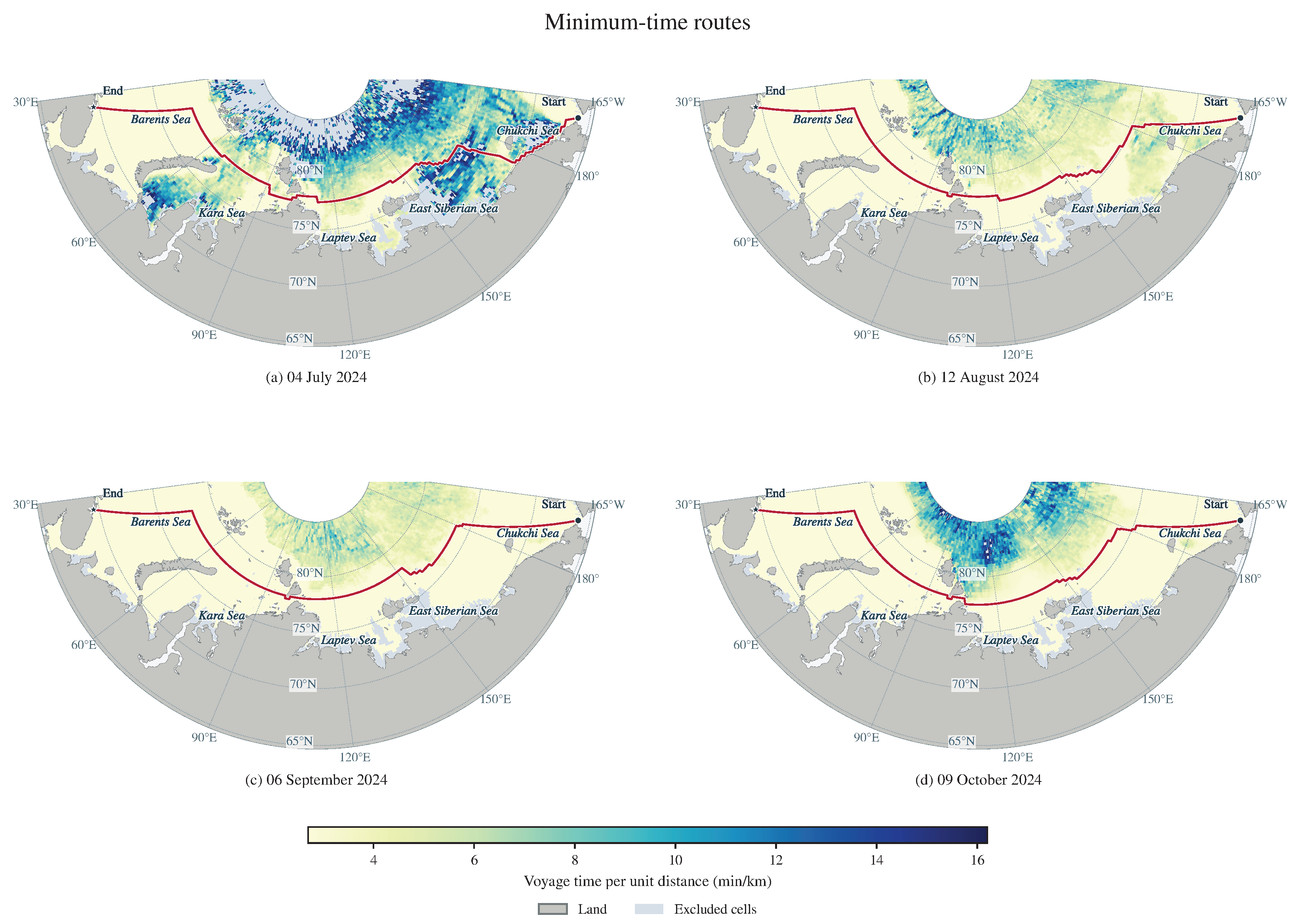
Selecting the route with the minimum total voyage time yields the representative routes in Figure 7. In Figure 7, Figure 8 and Figure 9, panels (a)–(d) correspond to 4 July, 12 August, 6 September, and 9 October 2024, respectively. In Figure 7, red lines indicate the representative minimum-time routes, and circles and stars mark the start and end points, respectively. The background shows the voyage time per unit distance for each grid cell under the L1 forecast field initialized on the corresponding date. It is calculated as in min/km, where v is the local vessel speed in kn calculated by the vessel model. Voyage distance, voyage time, propulsion fuel consumption, cumulative ice-condition severity, and window CVaR are summarized in Table 7.
Table 7.
Evaluation results for the representative minimum-time routes.
The minimum-time routes follow broadly similar corridors across the four dates, but differences in sea ice conditions along the routes produce marked variations in voyage time and cumulative ice-condition severity (Figure 7 and Table 7). The minimum-fuel solutions and the solutions with minimum cumulative ice-condition severity below are compared with the minimum-time solution initialized on the same date to quantify the costs associated with improvements in each objective.
Figure 7.
Representative minimum-time routes and voyage time per unit distance for four initialization dates: (a) 4 July, (b) 12 August, (c) 6 September, and (d) 9 October 2024.
4.4.2. Representative Minimum-Fuel Routes
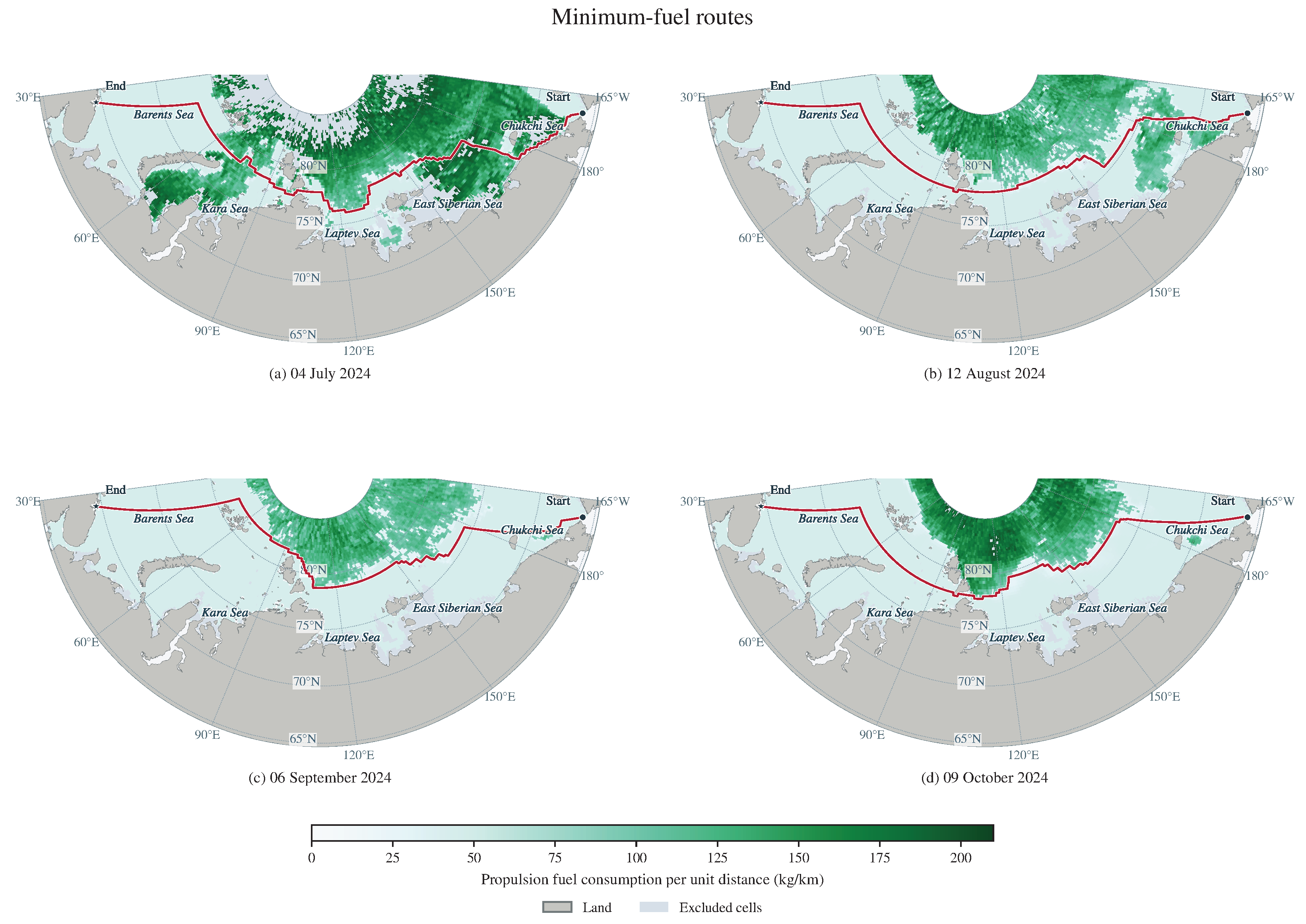
Selecting the route with the minimum total propulsion fuel consumption yields the representative routes shown in red in Figure 8. The background uses a linear color scale to show propulsion fuel consumption per unit distance in each grid cell under the L1 forecast field initialized on the corresponding date. It is calculated as in kg/km, where f is the propulsion fuel consumption rate in t/h. Route evaluation results are listed in Table 8.
Table 8.
Evaluation results for the representative minimum-fuel routes.
By adjusting local route alignments, the minimum-fuel routes produce different combinations of voyage distance, vessel speed, and propulsion power (Figure 8). Relative to the minimum-time solution initialized on the same date, propulsion fuel consumption decreases by 5.75–10.56% across the four dates, while voyage time increases by 17.691–29.871 h. Cumulative ice-condition severity and window CVaR both increase. In September, window CVaR increases from 2.0000 to 22.6090, indicating that fuel savings are accompanied by a greater failure burden in the tail of the scenario distribution (Table 7 and Table 8).
Figure 8.
Representative minimum-fuel routes and propulsion fuel consumption per unit distance for four initialization dates: (a) 4 July, (b) 12 August, (c) 6 September, and (d) 9 October 2024.
4.4.3. Representative Routes with Minimum Cumulative Ice-Condition Severity
Selecting the route with the minimum cumulative ice-condition severity over the complete route yields the representative routes shown in blue in Figure 9. The background uses a linear color scale from 0 to 1 to show the dimensionless local ice-condition severity score , which is determined by sea ice concentration and thickness. Route-level cumulative ice-condition severity is obtained by integrating this score over voyage time and is expressed in score·h. The evaluation results are given in Table 9.
Table 9.
Evaluation results for the representative routes with minimum cumulative ice-condition severity.
Figure 9.
Representative routes with minimum cumulative ice-condition severity and the local ice-condition severity score for four initialization dates: (a) 4 July, (b) 12 August, (c) 6 September, and (d) 9 October 2024.
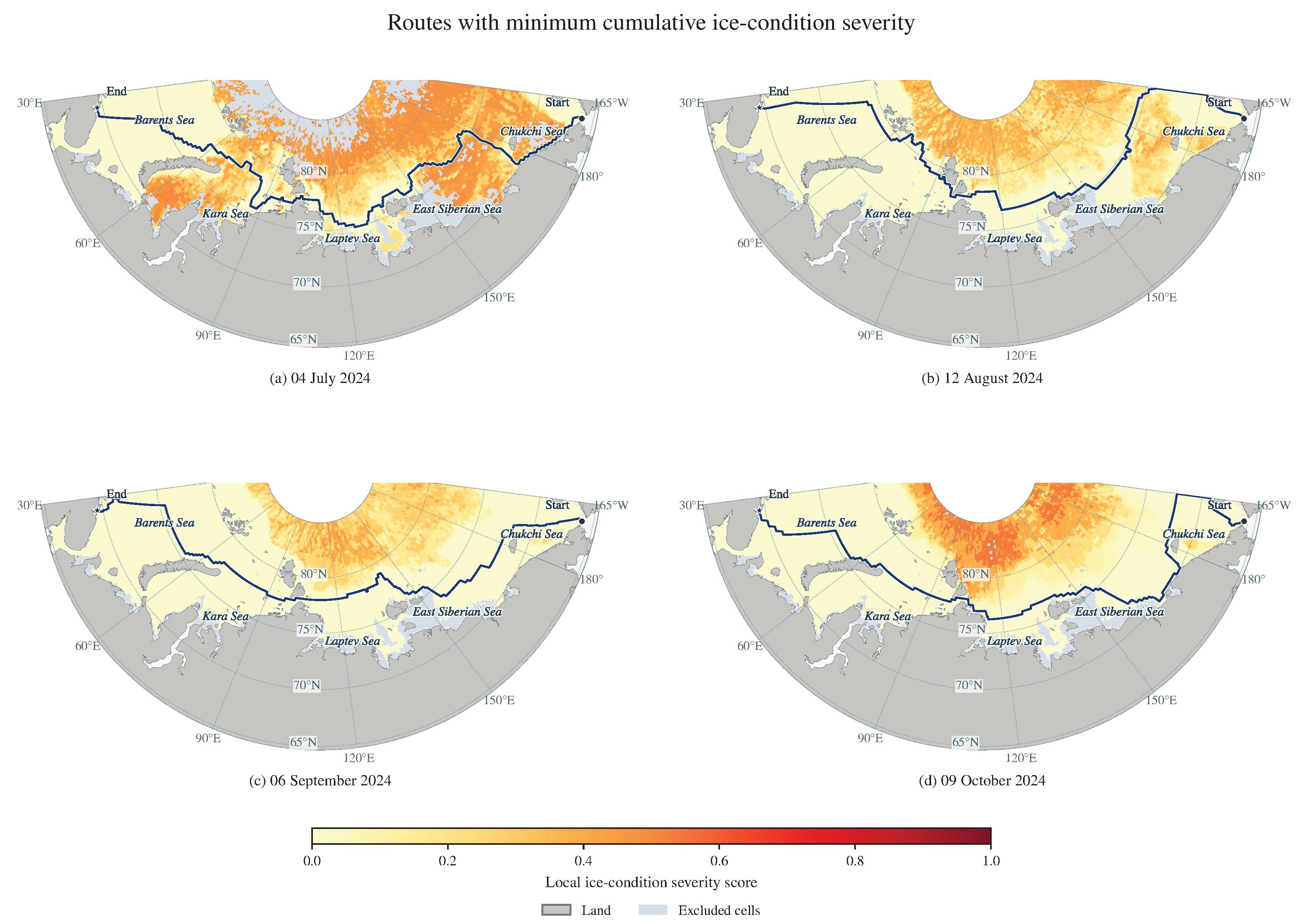
The representative routes with minimum cumulative ice-condition severity detour through areas with lower local ice-condition severity scores in several parts of the corridor, reducing cumulative ice-condition severity at the expense of longer voyage distances and times and greater propulsion fuel consumption (Figure 9 and Table 9). Relative to the minimum-time solutions, cumulative ice-condition severity decreases by 21.13–93.03% across the four dates, while voyage time increases by 13.72–26.10% and propulsion fuel consumption by 13.51–28.87%.
Reductions in cumulative ice-condition severity and changes in window CVaR do not occur in parallel. In July, the solution with minimum cumulative ice-condition severity reduces this metric by 21.13%, but window CVaR decreases by only approximately 1.52%. In October, cumulative ice-condition severity decreases by 78.03%, while window CVaR remains unchanged. These cases show that the two metrics provide different evaluation information. The next subsection examines how CVaR changes candidate retention and route selection.
4.5. Incremental Decision-Making Role of Path-Level CVaR
4.5.1. Candidate Nondominated Filtering and Four-Objective Trade-Offs
Within the common feasible candidate set for each date, adding CVaR increases the number of nondominated candidates from 8 to 13 in July and from 19 to 22 in September; the numbers remain unchanged in August and October (Table 10). The newly retained candidates are dominated in the three-objective evaluation, but their window CVaR values are lower than those of the routes that previously dominated them. They are, therefore, no longer dominated by those routes in the four-objective evaluation.
Table 10.
Candidate counts and nondominated filtering results for the four departure dates.
In the candidate set for 6 September 2024, candidate 24 has greater voyage time, propulsion fuel consumption, and cumulative ice-condition severity than candidate 4, but its window CVaR is lower, at 0.9023 compared with 2.0000 for candidate 4. Candidate 4 dominates candidate 24 in the three-objective evaluation, whereas neither dominates the other after CVaR is added. Filtering the complete candidate set further confirms that candidate 24 belongs to the four-objective nondominated set (Table 11). This comparison shows that window CVaR provides tail-risk information beyond the three voyage costs for candidate filtering.
Table 11.
Comparison of September candidates whose filtering outcome changes after window CVaR is introduced.
Figure 10 and Figure 11 present the four-objective trade-offs for 4 July and 6 September 2024, with 13 and 45 L1-feasible candidates, respectively. Panels (a) and (b) plot voyage time against propulsion fuel consumption and cumulative ice-condition severity. Marker area increases with window CVaR (). Both figures use a common area scale across dates and marker shapes, with axis ranges set separately.
Figure 10.
Four-objective trade-offs and representative candidate routes on 4 July 2024. (a) Voyage time and propulsion fuel consumption; (b) voyage time and cumulative ice-condition severity; (c) routes R0 and R23; (d) enlarged view of the boxed region.
Figure 11.
Four-objective trade-offs and representative candidate routes on 6 September 2024. (a) Voyage time and propulsion fuel consumption; (b) voyage time and cumulative ice-condition severity; (c) routes R4 and R24; (d) enlarged view of the boxed region. The insets in (a,b) use the units of the corresponding main axes.
Green circles, red triangles, and dark blue squares identify three-objective nondominated candidates, additional nondominated candidates retained after introducing window CVaR, and candidates dominated under four objectives, respectively. Black outlines and candidate identifiers link the scatterplots to the representative routes in panels (c) and (d). Green solid lines with circles and red dashed lines with triangles distinguish the two routes. Black boxes and arrows connect the overview maps to the enlarged local views. The September insets resolve the differences in voyage time, propulsion fuel consumption, and cumulative ice-condition severity between R4 and R24.
In July, compared with the minimum-time solution R0, the minimum-window-CVaR solution R23 reduces window CVaR by 18.55%, while increasing voyage time and propulsion fuel consumption under the fixed field by 12.72% and 13.71%, respectively, illustrating the trade-off between voyage costs and tail risk.
To examine the effect of the cost field, candidate routes and their window CVaR values are held fixed, while the first three objectives are recalculated using the L2–L7 point-forecast snapshots. Relative to L1, the Jaccard overlap of the four-objective fronts ranges from 0.111 to 0.280 in July, 0.167 to 0.480 in August, 0.409 to 0.677 in September, and 0.477 to 0.710 in October, indicating that front composition is sensitive to the cost snapshot. In July, the feasible set also changes: only 13 candidates are feasible under L1, whereas all 49 are feasible under L2–L7. When filtering is repeated with the 13 routes feasible under all seven snapshots held fixed, the July front overlap is 0.538–0.923. Thus, the original differences reflect the effects of both changes in feasibility and changes in costs.
4.5.2. Changes in Route Selection at the Same State
The comparison uses 40 decision states recorded along the four voyages executed by strategy C, comprising 5, 12, 11, and 12 states for departures on 4 July, 12 August, 6 September, and 9 October 2024, respectively. At each state, the vessel position, environmental inputs, and feasible candidate set are held fixed, and the selection rules of D and C are applied separately. Successive states within each voyage are temporally dependent. The results provide a descriptive comparison of route selection along these four C trajectories. The two rules select different routes at eight states. In all eight cases, four-objective selection reduces the predicted window CVaR while increasing predicted propulsion fuel consumption; it also reduces predicted voyage time in five cases and predicted cumulative ice-condition severity in seven cases. In Table 12, day index 0 denotes the departure day, candidate arrows point from the route selected by the three-objective rule to that selected by the four-objective rule, and all differences are calculated as the four-objective value minus the three-objective value.
Table 12.
Differences in predicted metrics between four- and three-objective selection at the same state.
Figure 12 compares the complete planned routes selected by the three- and four-objective rules from the same candidate set at each departure state. Green dashed lines with circles denote D, and red dotted lines with triangles denote C. Black frames and arrows link the overview maps to the enlarged local views. The background shows water depth, with land in gray. Dark circles and squares mark the departure and destination, respectively.
Figure 12.
Planned routes selected by the three-objective (D) and four-objective (C) rules at departure: (a) 12 August and (b) 6 September 2024. Each overview is paired with an enlarged local view.
In August, adding CVaR shifts the route locally northward near W, whereas in September it shifts the route locally southward near E. In both cases, lower window CVaR is obtained at the cost of greater predicted propulsion fuel consumption, showing how the risk objective changes the cost–risk trade-off of the complete route through adjustments to local segments (Figure 12 and Table 12).
4.6. Full-Voyage Comparison of Static and Receding-Horizon Strategies with Continuous Vessel Positions
Section 4.5 examines how path-level window CVaR affects candidate evaluation and route selection at the same decision state. The full-voyage evaluation comprises 64 simulations under strategies S, D, C, and EC for 16 departure dates in 2024. The four original departure cases are examined in detail, and Section 4.6.5 summarizes termination states and date-paired execution costs for the expanded evaluation. Comparing D with S evaluates the effects of receding-horizon updates on voyage outcomes. Comparing C with D evaluates the effects of adding path-level window CVaR to route selection. Comparing C with EC evaluates the effects of risk aggregation on executed tracks and cumulative costs.
4.6.1. Voyage Termination States, Execution Costs, and Window Risk
Table 13 summarizes the 16 simulated voyages under strategies S, D, C, and EC for the four original departure dates. Voyage time, propulsion fuel consumption, and cumulative ice-condition severity are obtained from voyage replay. Maximum path-level window CVaR and minimum RRI are calculated from daily predictive evaluations of the selected complete remaining route. All four strategies reach the destination for the August–October departures, allowing full-voyage execution costs to be compared. For the July departure, S reaches the destination. Strategies D and C terminate following navigability-constraint violations, and EC terminates when no admissible candidate route is available at a replanning step. Execution costs for these three incomplete voyages are reported up to termination.
Table 13.
Simulated voyage results for strategies S, D, C, and EC at the four original departure dates in 2024.
Across the 15 departure dates with completed voyages under all four strategies, waiting time is zero. Adding waiting fuel to the recorded trajectories, therefore, preserves fuel totals and strategy rankings at each date across all tested consumption rates. For the 4 July departure, S reaches the destination with 263.483 h of waiting. At , the additional waiting fuel is 26.348 t, giving an adjusted fuel consumption of 386.897 t. D and C each accumulate 21.832 h of waiting and 87.754 t of adjusted fuel consumption up to termination following a navigability-constraint violation. EC accumulates 19.214 h of waiting and 94.917 t of adjusted fuel consumption up to termination when no admissible action is available. The adjusted fuel values for D, C, and EC use the same waiting-fuel rate.
Figure 13 shows the executed tracks of strategies S, D, C, and EC for the four departure dates. The background is the L1 sea ice concentration forecast field for the corresponding departure date, with a common color scale from 0 to 100% across panels. Black rectangles identify the regions shown in the enlarged views below. Arrows connect each rectangle to its corresponding enlarged view, which includes a scale bar. Colors, line styles, and markers distinguish the strategies. Red crosses mark the July termination location of strategies D and C following navigability-constraint violations. Purple plus signs mark the July termination location of strategy EC when no admissible action is available. Route divergence is more pronounced in August. In September, the overall tracks are similar, although local differences in route selection remain.
Figure 13.
Executed tracks of strategies S, D, C, and EC and sea ice concentration forecasts at departure: (a) 4 July, (b) 12 August, (c) 6 September, and (d) 9 October 2024.
The dynamic three-objective strategy D is first compared with the static three-objective strategy S to examine the effects of daily receding-horizon updates. In August, D reduces cumulative ice-condition severity by 51.28% relative to S and increases the minimum window RRI from 0.602 to 0.639, but voyage time and propulsion fuel consumption increase. In October, D reduces voyage time by 3.613 h, cumulative ice-condition severity by 35.23%, and maximum window CVaR from 9.008 to 5.654, while the minimum window RRI decreases from 0.722 to 0.699. In September, execution costs and window-risk metrics are broadly similar for the two strategies (Table 13).
The dynamic four-objective strategy C is then compared with the dynamic three-objective strategy D to examine the risk and cost changes associated with introducing CVaR. In August, C reduces maximum window CVaR from 6.203 to 5.053 and increases minimum window RRI from 0.639 to 0.677. At the same time, voyage time decreases by 0.738 h, propulsion fuel consumption increases by 3.016 t, and cumulative ice-condition severity increases by 14.81%. In September and October, maximum window CVaR decreases from 4.053 to 2.902 and from 5.654 to 4.000, respectively, while minimum window RRI remains unchanged in both cases. Execution costs differ only slightly between the two strategies in September; in October, their executed tracks and cumulative execution costs are identical (Table 13).
Comparing EC with C shows how risk aggregation affects voyage outcomes (Table 13). For the August and September departures, EC produces lower maximum path-level window CVaR and higher minimum RRI. In August, EC also reduces propulsion fuel consumption and cumulative ice-condition severity, with a 0.180 h increase in voyage time. In September, EC reduces cumulative ice-condition severity, with increases in voyage time and propulsion fuel consumption. In October, EC reduces voyage time, propulsion fuel consumption, and cumulative ice-condition severity. The two strategies have equal maximum path-level window CVaR and minimum RRI for that departure.
4.6.2. Receding-Horizon Risk Changes and Differences Between Planning and Execution
Table 13 reports the maximum window CVaR for each voyage. Figure 14 further shows how the window CVaR of the selected remaining route changes across decision days. The horizontal axis gives the number of days since departure, with 0 denoting the departure decision. Figure 14a uses a separate vertical-axis range and includes an inset showing risk changes during days 0–4. Figure 14b–d uses a common vertical-axis range to facilitate comparison of risk levels across the August–October cases. Each strategy’s curve ends at its last decision before voyage termination. In Figure 14a, the gray vertical line marks the termination of strategies D and C at 119.456 h following navigability-constraint violations. The purple vertical line marks the termination of strategy EC at 120 h when no admissible action is available.
Figure 14.
Daily path-level window of the selected remaining routes under strategies S, D, C, and EC for four departure cases: (a) 4 July, (b) 12 August, (c) 6 September, and (d) 9 October 2024.
In October, the dynamic three- and four-objective strategies select remaining routes with window CVaR values of 5.654 and 0.301, respectively, at departure, but the segments executed on the first day are identical. Following the next day’s update, both strategies select the same subsequent route, ultimately producing identical executed tracks and cumulative costs. The values 5.654 and 4.000 in Table 13 are the maximum window CVaR values across all decision records for the two strategies and, therefore, represent a different summary from the departure values. Thus, the lower maximum window CVaR in this case reflects differences in the predicted risk of the remaining planned routes.
4.6.3. Receding-Horizon Execution in the July Case
Figure 15 presents the local execution sequence of strategies D and C for the July departure in chronological order, with all times measured from departure. All panels share the same map extent, scale, and color scale; the background shows the reference equivalent ice thickness at the corresponding time. Dark solid lines show the executed tracks, purple dashed lines show the unexecuted portions of the currently selected routes, and vessel-shaped markers indicate the current positions.
Figure 15.
Local execution sequence of strategies D and C in the July departure case: (a) waiting at 74.952 h, (b) replanning at 96 h, (c) underway at 108 h, (d) waiting at 118.672 h, and (e) termination at 119.456 h.
In July, the first four decisions and the corresponding execution are identical for strategies D and C. Both start waiting at N, E at 74.952 h after departure (Figure 15a). At 96 h, the dynamic three-objective strategy D and dynamic four-objective strategy C select candidates 25 and 35, respectively, at the fifth decision, with predicted window CVaR values of 43.466 and 40.165. Although the complete routes differ, the local segments subsequently executed remain identical (Figure 15b,c). At 118.672 h, the vessel reaches N, E and starts waiting again; the reference equivalent ice thickness in the occupied grid cell is approximately 1.194 m (Figure 15d). At 119.456 h, this value reaches the 1.200 m threshold. The location is classified as unnavigable according to the navigability state following the threshold event, and both strategies terminate because of a navigability-constraint violation at the current position (Figure 15e). The point forecast for that decision cycle gives an equivalent ice thickness of approximately 1.028 m at the same location and time.
The static strategy, by contrast, reaches the destination at 629.647 h after a cumulative waiting time of 263.483 h (Table 13).
4.6.4. Cost Estimation and Execution Consistency Checks
For the four original departure dates, 19 of the 40 decisions under strategy C include a nonzero terminal voyage-time estimate, concentrated in the first four or five decisions of each voyage. The maximum shares of terminal voyage time and propulsion fuel consumption in their respective estimated costs for the complete remaining route are 52.65% and 49.95%, respectively (Table 14). The maximum for each metric is calculated separately and need not occur at the same decision. In the completed August–October voyages, the terminal terms become zero at later decisions as the remaining route shortens.
Table 14.
Frequency and cost shares of terminal estimates under the four-objective strategy.
Numerical convergence is checked using progressive refinement. The along-route geometric sampling steps at the first two levels are 0.125 and 0.0625 km, respectively, and the environmental-field time discretization steps are 0.375 and 0.1875 h. Adjacent levels must produce the same execution or prediction status, with an endpoint-position difference no greater than 1 m. Continuous quantities, including voyage time, propulsion fuel consumption, cumulative ice-condition severity, and voyage distance, must satisfy , where and are the values of the same metric at the earlier and later refinement levels, respectively, and errors are evaluated in that metric’s original units. Candidate evaluations additionally require consistent availability, terminal-estimation status, and event classifications for each scenario member; the failed length for each member must satisfy the same error bound. Across the 12 voyages of S, D, and C for the four original departure dates, all 142 daily execution-update calculations and 2568 candidate evaluations pass the checks at the second refinement level, with a maximum execution-endpoint difference of approximately 0.594 m. Inputs for each new day agree with the actual terminal state of the previous day, with no vessel-position resets or losses of cumulative quantities detected.
4.6.5. Expanded Evaluation Across Departure Dates
Table 15 summarizes the termination states of 64 simulations across 16 departure dates in 2024. Strategy S reaches the destination for all 16 departures; D, C, and EC each reach the destination for 15 departures. The three other terminations occur for the 4 July departure: D and C terminate following navigability-constraint violations, and EC terminates when no admissible action is available. All four strategies reach the destination for the remaining 15 departure dates, providing matched full-voyage comparisons of execution costs.
Table 15.
Voyage termination states across 16 departure dates in 2024.
Table 16 reports date-paired differences in execution costs for the 15 departure dates on which all four strategies reach the destination. All 60 voyages in this comparison have zero waiting time. For comparison A–B, each difference is calculated as the value for strategy A minus that for strategy B at the same departure date; negative values indicate lower costs under A. Each table entry gives the arithmetic mean of these differences, followed by [minimum, maximum]. The comparisons are summarized descriptively, with temporal dependence between nearby departure dates.
Table 16.
Date-paired differences in full-voyage execution costs across 15 departure dates in 2024.
Across the 15 departure dates with completed voyages under all four strategies, D and C have lower mean voyage time, propulsion fuel consumption, and cumulative ice-condition severity than S (Table 16). Relative to S, C reduces cumulative ice-condition severity for all 15 dates, voyage time for 14 dates, and propulsion fuel consumption for 11 dates. Compared with D, C reduces mean cumulative ice-condition severity by 0.379 score·h, accompanied by mean increases of 0.138 h in voyage time and 0.598 t in propulsion fuel consumption.
Compared with EC, C has lower mean voyage time, propulsion fuel consumption, and cumulative ice-condition severity by 0.791 h, 0.843 t, and 0.215 score·h, respectively. C and EC produce identical values for all three execution costs on six departure dates. For each of voyage time and propulsion fuel consumption, C has a lower value on six dates and a higher value on three dates. Cumulative ice-condition severity is lower under C on three dates and higher on six dates. These date-specific comparisons show how the two risk aggregation methods produce different trade-offs among realized voyage costs.
4.7. Auxiliary Evaluation and Module Validation
Following Section 3.5, this subsection examines the ability of RRI to distinguish candidate routes, the consistency of LPA* search results, and navigability and the continuous execution interface after path smoothing. The sample size is reported separately for each validation.
4.7.1. Ability of RRI to Distinguish Candidate Routes
RRI is evaluated using candidate routes from an archived experiment with five route-selection rules: deterministic look-ahead, priority to expected failure loss, priority to path-level window CVaR, and fixed-scale three- and four-objective selection. Each rule is applied to departures on 4 July, 12 August, 6 September, and 9 October 2024, yielding 20 simulated voyages, 231 decision-state records, and 6767 candidate-route records. All five rules share candidate-generation and feasibility-screening procedures, dynamic cost evaluation, and an execution scheme with a maximum rate-interpolation interval of 0.75 h. Their voyage outcomes are compared within this archived experiment. Table 17 summarizes the voyage outcomes of the five route-selection rules.
Table 17.
Archived voyage results for five route-selection rules at four departure dates in 2024.
For the July departure, EL and CV reach the destination, and DL, F3, and F4 terminate following navigability-constraint violations (Table 17). Among the two completed voyages, EL has lower voyage time, propulsion fuel consumption, waiting time, and cumulative ice-condition severity. All five rules reach the destination without waiting for the August–October departures. In August and September, EL and CV produce identical execution costs and the lowest cumulative ice-condition severity, together with longer voyage times and higher propulsion fuel consumption than DL, F3, and F4. In October, F4 achieves the shortest voyage time and lowest propulsion fuel consumption, and DL achieves the lowest cumulative ice-condition severity.
The path-smoothing and continuous-interface validation in Section 4.7.3 also uses the same 231 states and their selected remaining routes as initial inputs. RRI is calculated for these candidate routes according to Section 3.5.1; the results are shown in Figure 16. Figure 16 shows the RRI values of 48 candidate routes at the departure state on 12 August 2024, ordered by increasing RRI, with each point representing one route.
Figure 16.
Window RRI values of 48 candidate routes at the departure state on 12 August 2024, ordered by increasing RRI.
Candidate RRI values in the example state range from 0.293 to 0.977. Across the archived states, candidate RRI values differ in more than half of the decision states.
4.7.2. Consistency Validation of LPA* Incremental Search
Following the setup in Section 3.5.2, replay at fixed decision states and paired-voyage experiments are conducted to compare the search and execution results of full A* recomputation and LPA* (Figure 17).
Figure 17.
Consistency validation of full A* recomputation and LPA* through fixed-state replay and paired-voyage experiments.
Across 1960 searches at 40 fixed decision states, the two algorithms produce identical reachability results, route node sequences, and search-objective values. The candidate sets are also identical at all 40 states. In four paired-voyage experiments covering the four departure dates, daily route selections and termination states match exactly, and the recorded differences in vessel position and cumulative costs are all zero, satisfying the numerical verification criteria of an absolute tolerance of and a relative tolerance of .
4.7.3. Path Smoothing and Continuous-Position Interface Validation
In Figure 18, blue dashed lines denote the original grid paths, and red solid lines denote the paths smoothed using cubic B-splines. Black boxes identify the regions around the largest local turning angle in the eastern corridor, and the insets show the corresponding local details. The background shows water depth, and gray denotes land. The percentages indicate changes in voyage distance and cumulative turning angle for the complete smoothed path relative to the original path.
Figure 18.
Initial routes under the CVaR-priority rule and their smoothing results for four departure dates: 4 July and 12 August 2024 (upper row), and 6 September and 9 October 2024 (lower row).
For all four departure dates, smoothing preserves the overall route alignment while replacing local corners with continuous curve transitions. Both voyage distance and cumulative turning angle decrease.
All 231 historically selected routes pass static geometric certification after cubic B-spline smoothing. Seven frozen environmental snapshots yield 1617 paired comparisons, of which 1601 have feasible original routes; all remain feasible after smoothing. The other 16 cases are already infeasible before smoothing. To reduce the influence of curve discretization on the comparison, risk is recalculated using CVaR of failed length, reported separately from the CVaR of failed-edge counts used in the main voyage experiments. After smoothing, CVaR of failed length decreases for 74 routes, remains unchanged for 150, and increases for 7.
In the continuous-position interface validation, short-term execution checks pass at all 231 historical states. Of these, 211 cases that remain active after execution also pass curve-to-grid reconnection and paired single-update validation. Vessel position, executed distance, and cumulative costs remain continuous through execution and reconnection, allowing subsequent grid-based planning to continue from the actual terminal state reached along the smoothed route.
For risk evaluation of reconnected routes, the common prefix consists of the retained and connecting portions from the current vessel position to the grid reconnection point. Using failed length as the loss, evaluation of the grid-path suffix alone is compared with evaluation of the common prefix and suffix combined within the same scenario, and at least one candidate pair exhibits a strict reversal in CVaR ranking in each of 29 states. Although the common prefix is identical for all candidates at a given state, its loss still varies across sea ice scenarios. Adding it to the losses of different suffixes can change the composition of the tail scenarios that determine CVaR. Therefore, risk evaluation in continuous replanning must preserve the scenario correspondence between the prefix and suffix: the complete-route loss must first be formed for each member, and path-level CVaR must then be calculated across members.
5. Discussion
5.1. Relationship Between Predicted Risk and Realized Voyage Performance
Path-level window CVaR is the weighted mean of the failed-edge count over the worst 5% of scenario probability mass. It summarizes the tail of the seven-day window failure loss across the complete remaining route. Cumulative ice-condition severity integrates local ice-condition severity scores along the route over sailing and waiting time. Including window CVaR in nondominated filtering can retain candidates dominated under the three original objectives and alter the route selected for execution.
Realized voyage performance depends on the sequence of executed route segments and the reference ice conditions encountered during replay. For the original August departure, D and C reduce cumulative ice-condition severity relative to S, with increases in voyage time and propulsion fuel consumption. In October, D and C execute the same first-day segment and select the same route at the next update, producing identical executed tracks and cumulative costs alongside different maximum path-level window CVaR values. At the fifth July decision, C selects a route with lower path-level window CVaR than D. Both strategies subsequently terminate when the occupied grid cell becomes unnavigable. Strategy S reaches the destination with 263.483 h of cumulative waiting. Across the 15 departure dates with completed voyages under all four strategies, C has lower mean cumulative ice-condition severity than D, with higher mean voyage time and propulsion fuel consumption (Table 16). Relative to EC, C has lower mean values for all three execution costs; the direction and magnitude of the differences vary across departure dates. These comparisons show how risk-sensitive route selection changes the balance among execution costs under the evaluated departure conditions.
5.2. Differences from Representative Arctic Route-Planning Research
Table 18 compares the present framework with the multi-objective route-planning framework of Liu et al. [10] and the CVaR-based stochastic shortest-path formulation of Sibul et al. [5]. The comparison covers environmental inputs, optimization objectives, risk evaluation, route updates, and solution methods.
Table 18.
Comparison of the present framework with those of Liu et al. [10] and Sibul et al. [5].
Sibul et al. [5] formulate a risk-averse stochastic shortest-path problem that minimizes a weighted sum of expected transit time and the CVaR of total transit time. Their scenario losses are evaluated for complete routes before departure. The present framework constructs seven-day sea ice scenarios from point forecasts and paired historical residuals, and defines scenario loss as the number of remaining-route edges that become unnavigable within that window. Window CVaR enters four-objective route selection alongside voyage time, propulsion fuel consumption, and cumulative ice-condition severity. Receding-horizon planning updates the route using new forecasts and the vessel’s current position, with an execution horizon of up to 24 h.
5.3. Scope of the Study and Future Extensions
The paired scenarios preserve the correspondence of historical residual members across sea ice variables, spatial locations, and forecast lead times. The 2024 evaluation shows improved marginal prediction-interval coverage and lower energy and variogram scores at the sampled grid cells and adjacent pairs. These diagnostics assess marginal calibration and multivariate forecast performance at the evaluated spatial configurations. Path-level window CVaR has a distinct validation target: the upper tail of the window failure-loss distribution for the complete remaining route.
The vessel is represented by one parameterized model, and the route fuel cost is main-propulsion consumption. Application to a particular ship requires calibration against recorded speed, power, and fuel consumption. The waiting-fuel sensitivity analysis applies prescribed consumption rates for auxiliary engines and station keeping to fixed execution trajectories and evaluates the resulting fuel totals and rankings (Section 4.6.1).
The full-voyage evaluation covers 16 departure dates in 2024, with the forecasting model, scenario calibration, vessel parameters, and strategy-specific settings held fixed across dates. Strategy comparisons are paired by departure date and summarized descriptively. Nearby departures share portions of the environmental time series, and daily decision states form repeated observations within each voyage. Further evaluation across years and vessel configurations can assess the transferability of these findings. Terminal-cost shares are high early in the voyages, and both the planning-window length and the environmental assumptions used for that terminal cost affect the selected route.
6. Conclusions
This study proposes a multi-objective route-planning method for the time-varying sea ice environment of the Northeast Passage that integrates seven-day sea ice forecasts, paired scenarios, path-level CVaR, and receding-horizon planning with continuous vessel positions. By preserving scenario correspondence across sea ice variables, spatial locations, and forecast lead times, the method converts forecast errors into a distribution of failure losses for the complete remaining route over a seven-day window and evaluates this risk jointly with voyage time, propulsion fuel consumption, and cumulative ice-condition severity.
Candidate screening and same-state comparisons measure the change in route selection after path-level CVaR is added. After CVaR was included, some routes with a lower tail failure burden that were dominated under the original three objectives entered the nondominated set. The same-state comparison uses 40 decision states recorded along strategy C’s voyages for the four original departure dates. At these states, the selection rules of D and C choose different routes in eight cases. In all eight cases, C selects a route with lower predicted window CVaR and higher predicted propulsion fuel consumption than D. Predicted voyage time decreases in five cases and predicted cumulative ice-condition severity in seven.
The expanded evaluation comprises 64 simulations across 16 departure dates in 2024 using one parameterized Arc6-class Aframax tanker. S reaches the destination for all 16 departures, and D, C, and EC each reach the destination for 15 departures. For the 4 July departure, D and C terminate following navigability-constraint violations, and EC terminates when no admissible action is available. Across the 15 departure dates with completed voyages under all four strategies, C has lower mean voyage time, propulsion fuel consumption, and cumulative ice-condition severity than S. Relative to D, C reduces mean cumulative ice-condition severity by 0.379 score·h, with mean increases of 0.138 h in voyage time and 0.598 t in propulsion fuel consumption. Compared with EC, C has lower mean values for these three execution costs, with date-specific differences in the direction and magnitude of the changes.
Author Contributions
Conceptualization, J.F. and G.Y.; Methodology, J.F. and G.Y.; Software, J.F.; Validation, J.F.; Formal analysis, J.F.; Investigation, J.F.; Resources, G.Y.; Data curation, J.F.; Writing–original draft, J.F.; Writing–review and editing, J.F.; Visualization, J.F.; Supervision, G.Y. All authors have read and agreed to the published version of the manuscript.
Funding
This research received no external funding.
Data Availability Statement
The publicly available data used in this study can be obtained from the Copernicus Marine Service (https://marine.copernicus.eu), NSIDC (https://nsidc.org), the Copernicus Climate Data Store (ERA5; https://cds.climate.copernicus.eu), GEBCO (https://www.gebco.net), and Natural Earth (https://www.naturalearthdata.com). The implementation code, trained ConvLSTM model weights, and processed route results are available from the corresponding author upon reasonable request.
Conflicts of Interest
The authors declare no conflicts of interest.
Appendix A. Seven-Day ConvLSTM Sea Ice Forecasting Model and Training Settings
Inputs and outputs. The model input is an eight-channel sequence of environmental grids spanning seven consecutive days, with a spatial grid size of . The input channels comprise M4S-corrected sea ice concentration, sea ice thickness, 10 m zonal and meridional winds, 2 m air and dewpoint temperatures, low cloud cover, and total cloud cover. The input tensor for a single sample has dimensions , corresponding, in order, to historical time, variable channels, and the two spatial dimensions. The output dimensions are , corresponding to sea ice concentration and thickness for forecast days 1–7. Each variable is standardized using the mean and standard deviation calculated from the 2019–2021 training data.
Network architecture. The model consists of a two-layer ConvLSTM encoder and two convolutional output heads. Each encoder layer has 16 hidden channels and a convolutional kernel, with padding used to preserve the spatial dimensions. The encoder extracts spatiotemporal features from the seven-day historical sequence, and the hidden state of the second layer at the final time step serves as the shared feature representation. The two output heads directly predict sea ice concentration and thickness for days 1, 3, and 5 and days 2, 4, 6, and 7, respectively. These outputs are ordered by forecast lead time to form daily forecasts for all seven days.
Staged training. In the first stage, the encoder and the output head for days 1, 3, and 5 are trained jointly using 405 training samples from 2019–2021. The parameters at epoch 30 are selected based on 135 model-selection samples from 2022. In the second stage, these parameters are frozen, and the output head for days 2, 4, 6, and 7 is trained using 399 training samples from 2019–2021. The parameters at epoch 2 are selected based on 133 model-selection samples from 2022. The maximum forecast lead times in the two stages are five and seven days, respectively, resulting in different numbers of available samples.
Loss function and optimization settings. In both stages, the Smooth L1 loss is computed in the standardized variable space over valid ocean grid cells, with area weights proportional to the cosine of latitude. Equal weights are assigned to the two sea ice variables and to the forecast lead times trained in each stage. The optimizer is AdamW [40], with a learning rate of 0.001, a weight decay of 0.0001, a batch size of 1, and a maximum of 50 training epochs. Early stopping is based on the loss on the 2022 model-selection set, with a patience of 8 epochs and a minimum improvement of 0.0001. The gradient norm clipping threshold is 1.0, and the random seed is 20,260,915.
Model application. After training and model selection, the network parameters, standardization parameters, and M4S correction parameters are fixed. The network outputs are first transformed back to physical units by reversing standardization; sea ice concentration is then clipped to , and thickness is constrained to be nonnegative. The resulting point forecasts are used consistently for forecast performance evaluation, construction of historical residuals and state features, and candidate route evaluation. Concentration and thickness are not jointly set to zero at the point-forecast stage; consistency of the ice-free state in scenario fields is enforced as described in Section 3.1. Data from 2023 are used to construct the seven-day forecast residual archive and to fit and freeze the scenario calibration parameters. Data from 2024 are used for forecast performance evaluation and voyage replay.
Appendix B. List of Symbols
Table A1.
Main symbols and their meanings.
References
- Wu, A.; Che, T.; Chen, J.; Zhu, X.; Xu, Q.; Dou, T.; Zhang, R.; Chen, S.; Wang, J.; Guo, Y. RouteView 2.0: A real-time operational planning system for vessels on the Arctic Northeast Passage. Environ. Model. Softw. 2025, 191, 106464. [Google Scholar] [CrossRef] [Scilit]
- Fu, S.; Zhang, D.; Montewka, J.; Yan, X.; Zio, E. Towards a probabilistic model for predicting ship besetting in ice in Arctic waters. Reliab. Eng. Syst. Saf. 2016, 155, 124–136. [Google Scholar] [CrossRef] [Scilit]
- Lehtola, V.V.; Montewka, J.; Goerlandt, F.; Guinness, R.; Lensu, M. Finding safe and efficient shipping routes in ice-covered waters: A framework and a model. Cold Reg. Sci. Technol. 2019, 165, 102795. [Google Scholar] [CrossRef] [Scilit]
- Ryan, C.; Huang, L.; Li, Z.; Ringsberg, J.W.; Thomas, G. An Arctic ship performance model for sea routes in ice-infested waters. Appl. Ocean Res. 2021, 117, 102950. [Google Scholar] [CrossRef] [Scilit]
- Sibul, G.; Schütz, P.; Fagerholt, K. Arctic route planning under ice uncertainty: A risk-averse stochastic shortest path problem. Transp. Res. Part E Logist. Transp. Rev. 2026, 205, 104507. [Google Scholar] [CrossRef] [Scilit]
- Liu, R.; Xue, Y.; Han, D.; Ni, B. Studies on model-scale ice using micro-potential-based peridynamics. Ocean Eng. 2021, 221, 108504. [Google Scholar] [CrossRef] [Scilit]
- Xue, Y.; Liu, R.; Li, Z.; Han, D. A review for numerical simulation methods of ship–ice interaction. Ocean Eng. 2020, 215, 107853. [Google Scholar] [CrossRef] [Scilit]
- Tian, S.; Bai, X.; Zemlyak, V.L.; Liu, R. Numerical model for the deformation of a viscoelastic ice plate under dynamic loading. Mar. Struct. 2026, 108, 104046. [Google Scholar] [CrossRef] [Scilit]
- Liu, R.; Luo, X.; Bai, X.; Semenov, D.A.; Zhang, J.; Zhang, L. Innovative experiments on ship resistance performance in managed ice floe fields. China Ocean Eng. 2025, 39, 58–72. [Google Scholar] [CrossRef] [Scilit]
- Liu, Y.; Lu, Y.; Xue, Y.; Ni, B.; Jiang, Y.; Guedes Soares, C. Multi-objective optimisation of arctic shipping routes considering navigational risk, voyage time, and fuel consumption. Reliab. Eng. Syst. Saf. 2026, 273, 112364. [Google Scholar] [CrossRef] [Scilit]
- Xu, T.; Yang, H.; Ma, J.; Xiong, K.; Hu, Q. An Improved D* Lite-Based Dynamic Route Planning Algorithm for Ships in Arctic Waters. J. Mar. Sci. Eng. 2024, 12, 2323. [Google Scholar] [CrossRef] [Scilit]
- Wu, A.; Che, T.; Li, X.; Zhu, X. Routeview: An intelligent route planning system for ships sailing through Arctic ice zones based on big Earth data. Int. J. Digit. Earth 2022, 15, 1588–1613. [Google Scholar] [CrossRef] [Scilit]
- Williams, T.; Korosov, A.; Rampal, P.; Ólason, E. Presentation and evaluation of the Arctic sea ice forecasting system neXtSIM-F. Cryosphere 2021, 15, 3207–3227. [Google Scholar] [CrossRef] [Scilit]
- Fetterer, F.; Knowles, K.; Meier, W.N.; Savoie, M.; Windnagel, A.K.; Stafford, T. Sea Ice Index, Version 4 (G02135); National Snow and Ice Data Center: Boulder, CO, USA, 2025. [Google Scholar] [CrossRef]
- Hersbach, H.; Bell, B.; Berrisford, P.; Hirahara, S.; Horányi, A.; Muñoz-Sabater, J.; Nicolas, J.; Peubey, C.; Radu, R.; Schepers, D.; et al. The ERA5 global reanalysis. Q. J. R. Meteorol. Soc. 2020, 146, 1999–2049. [Google Scholar] [CrossRef] [Scilit]
- Liu, Q.; Zhang, R.; Wang, Y.; Yan, H.; Hong, M. Daily Prediction of the Arctic Sea Ice Concentration Using Reanalysis Data Based on a Convolutional LSTM Network. J. Mar. Sci. Eng. 2021, 9, 330. [Google Scholar] [CrossRef] [Scilit]
- Fu, S.; Zhang, Y.; Zhang, M.; Han, B.; Wu, Z. An object-oriented Bayesian network model for the quantitative risk assessment of navigational accidents in ice-covered Arctic waters. Reliab. Eng. Syst. Saf. 2023, 238, 109459. [Google Scholar] [CrossRef] [Scilit]
- Zhang, X.; Zhou, Y.; Lu, Y.; Liu, Y.; Xue, Y.; Yu, X. A risk assessment model for ships besetting in ice along the Arctic Northeast Passage. Ocean Eng. 2025, 333, 121434. [Google Scholar] [CrossRef] [Scilit]
- Yu, Y.; Liu, K.; Fu, S.; Chen, J. Framework for process risk analysis of maritime accidents based on resilience theory: A case study of grounding accidents in Arctic waters. Reliab. Eng. Syst. Saf. 2024, 249, 110202. [Google Scholar] [CrossRef] [Scilit]
- Rockafellar, R.T.; Uryasev, S. Conditional value-at-risk for general loss distributions. J. Bank. Finance 2002, 26, 1443–1471. [Google Scholar] [CrossRef] [Scilit]
- Schefzik, R.; Thorarinsdottir, T.L.; Gneiting, T. Uncertainty Quantification in Complex Simulation Models Using Ensemble Copula Coupling. Stat. Sci. 2013, 28, 616–640. [Google Scholar] [CrossRef] [Scilit]
- Mayne, D.Q.; Rawlings, J.B.; Rao, C.V.; Scokaert, P.O.M. Constrained model predictive control: Stability and optimality. Automatica 2000, 36, 789–814. [Google Scholar] [CrossRef] [Scilit]
- GEBCO Bathymetric Compilation Group 2026. The GEBCO_2026 Grid—A Continuous Terrain Model for Oceans and Land at 15 Arc-Second Intervals; NERC EDS British Oceanographic Data Centre NOC: Liverpool, UK, 2026. [Google Scholar] [CrossRef]
- E.U. Copernicus Marine Service Information (CMEMS). Arctic Ocean Sea Ice Reanalysis (ARCTIC_MULTIYEAR_PHY_ICE_002_016); Marine Data Store (MDS); Mercator Ocean International: Toulouse, France, 2024. [Google Scholar] [CrossRef]
- Natural Earth. Land, 1:10 Million Scale [Data Set]. Available online: https://www.naturalearthdata.com/downloads/10m-physical-vectors/10m-land/ (accessed on 10 October 2026).
- de Leeuw, J.; Hornik, K.; Mair, P. Isotone Optimization in R: Pool-Adjacent-Violators Algorithm (PAVA) and Active Set Methods. J. Stat. Softw. 2009, 32, 1–24. [Google Scholar] [CrossRef] [Scilit]
- Shi, X.; Chen, Z.; Wang, H.; Yeung, D.-Y.; Wong, W.-K.; Woo, W.-C. Convolutional LSTM Network: A Machine Learning Approach for Precipitation Nowcasting. In Advances in Neural Information Processing Systems 28; Curran Associates, Inc.: Red Hook, NY, USA, 2015; pp. 802–810. [Google Scholar]
- Clark, M.; Gangopadhyay, S.; Hay, L.; Rajagopalan, B.; Wilby, R. The Schaake Shuffle: A Method for Reconstructing Space–Time Variability in Forecasted Precipitation and Temperature Fields. J. Hydrometeorol. 2004, 5, 243–262. [Google Scholar] [CrossRef] [Scilit]
- Hoerl, A.E.; Kennard, R.W. Ridge Regression: Biased Estimation for Nonorthogonal Problems. Technometrics 1970, 12, 55–67. [Google Scholar] [CrossRef]
- Topaj, A.; Tarovik, O. Ship route planning in simulation models of Arctic transport systems. In Proceedings of the 26th International Conference on Harbour, Maritime & Multimodal Logistics Modelling and Simulation (HMS 2024), Tenerife, Spain, 18–20 September 2024; p. 006. [Google Scholar] [CrossRef] [Scilit]
- Sibul, G.; Schütz, P. The impact of ice classing and ice conditions on the economics of Arctic shipping. In Proceedings of the 27th International Conference on Port and Ocean Engineering under Arctic Conditions (POAC 2023), Glasgow, UK, 12–16 June 2023. Paper 97. [Google Scholar]
- Holtrop, J.; Mennen, G.G.J. An approximate power prediction method. Int. Shipbuild. Prog. 1982, 29, 166–170. [Google Scholar] [CrossRef] [Scilit]
- Huang, L.; Li, Z.; Ryan, C.; Ringsberg, J.W.; Pena, B.; Li, M.; Ding, L.; Thomas, G. Ship resistance when operating in floating ice floes: Derivation, validation, and application of an empirical equation. Mar. Struct. 2021, 79, 103057. [Google Scholar] [CrossRef] [Scilit]
- Hart, P.E.; Nilsson, N.J.; Raphael, B. A Formal Basis for the Heuristic Determination of Minimum Cost Paths. IEEE Trans. Syst. Sci. Cybern. 1968, 4, 100–107. [Google Scholar] [CrossRef] [Scilit]
- Dijkstra, E.W. A note on two problems in connexion with graphs. Numer. Math. 1959, 1, 269–271. [Google Scholar] [CrossRef] [Scilit]
- Koenig, S.; Likhachev, M.; Furcy, D. Lifelong Planning A*. Artif. Intell. 2004, 155, 93–146. [Google Scholar] [CrossRef] [Scilit]
- Piegl, L.; Tiller, W. The NURBS Book, 2nd ed.; Springer: Berlin/Heidelberg, Germany, 1997. [Google Scholar] [CrossRef] [Scilit]
- Gneiting, T.; Raftery, A.E. Strictly Proper Scoring Rules, Prediction, and Estimation. J. Am. Stat. Assoc. 2007, 102, 359–378. [Google Scholar] [CrossRef] [Scilit]
- Scheuerer, M.; Hamill, T.M. Variogram-Based Proper Scoring Rules for Probabilistic Forecasts of Multivariate Quantities. Mon. Weather Rev. 2015, 143, 1321–1334. [Google Scholar] [CrossRef] [Scilit]
- Loshchilov, I.; Hutter, F. Decoupled Weight Decay Regularization. In Proceedings of the International Conference on Learning Representations (ICLR), New Orleans, LA, USA, 6–9 May 2019. [Google Scholar]
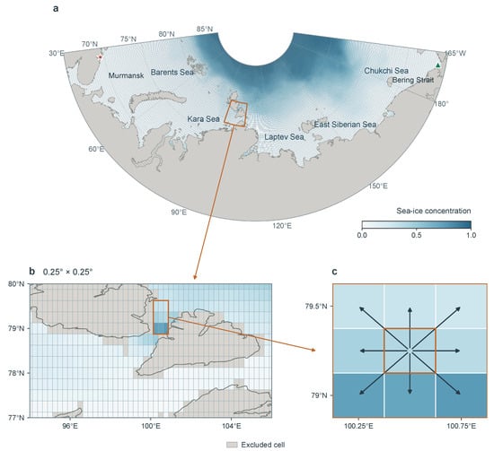
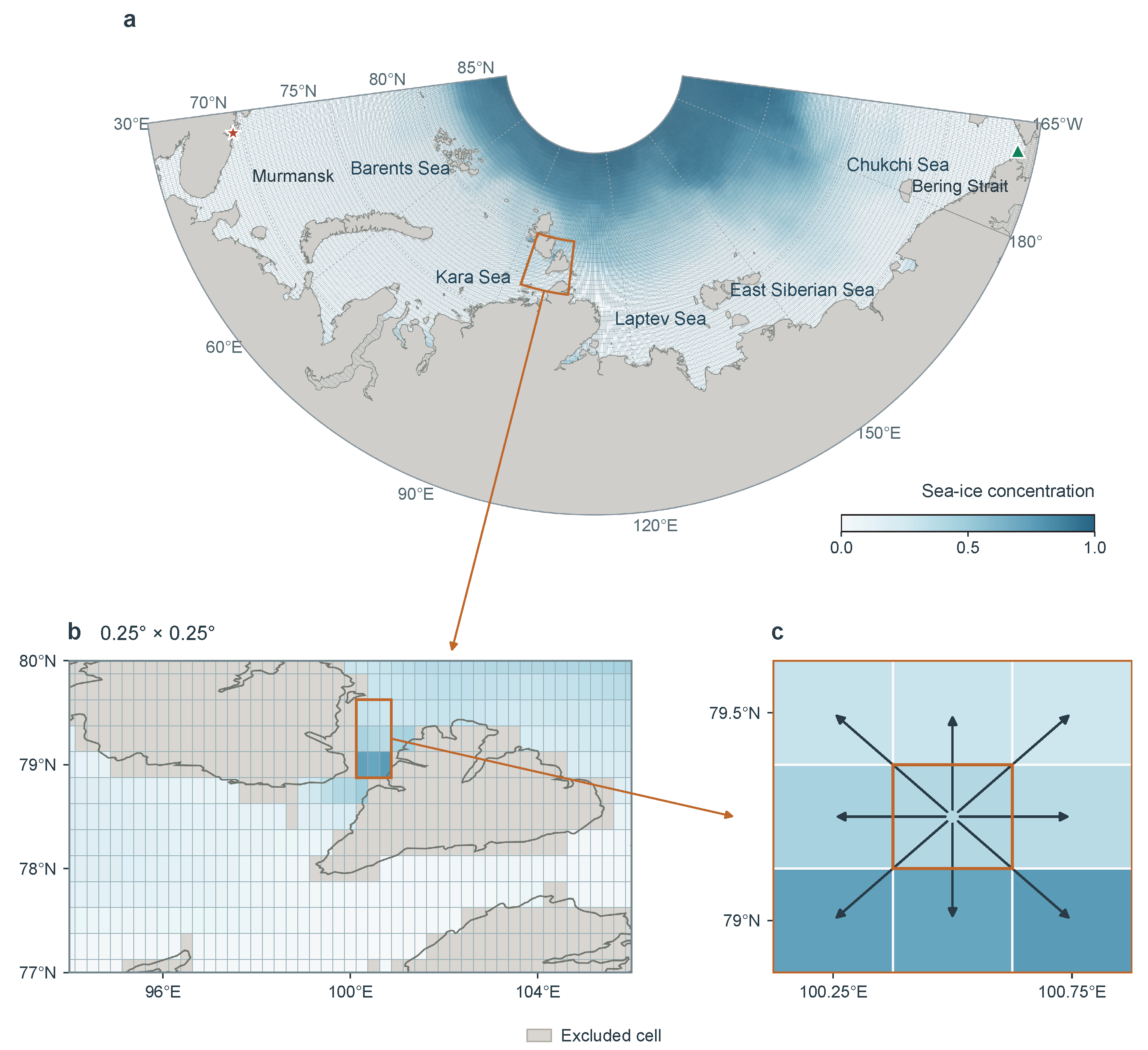
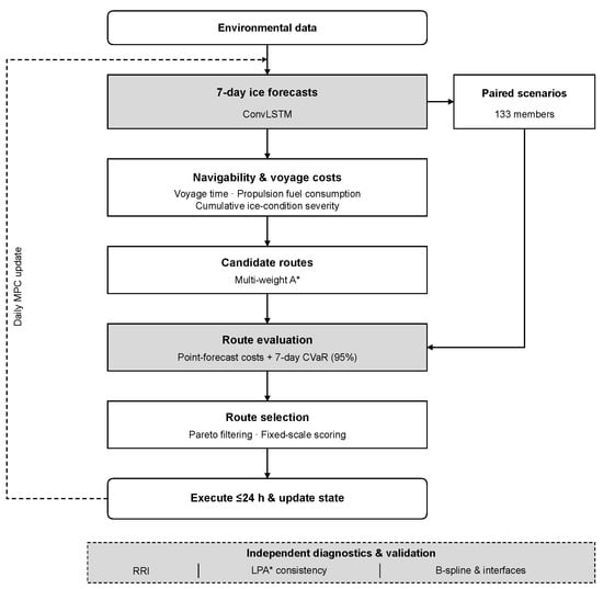
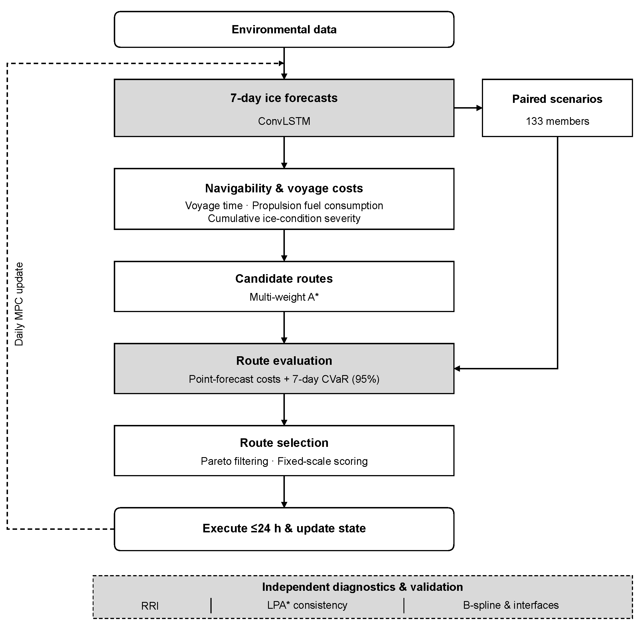
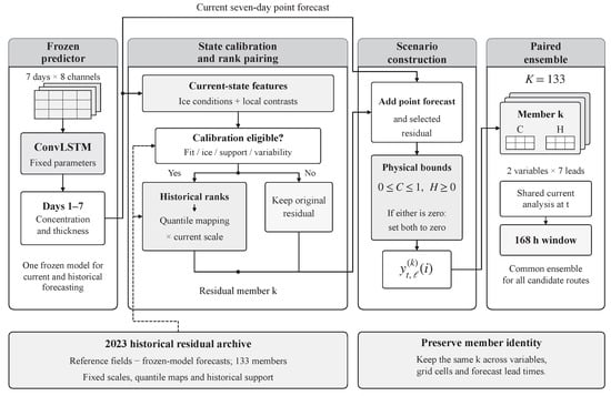
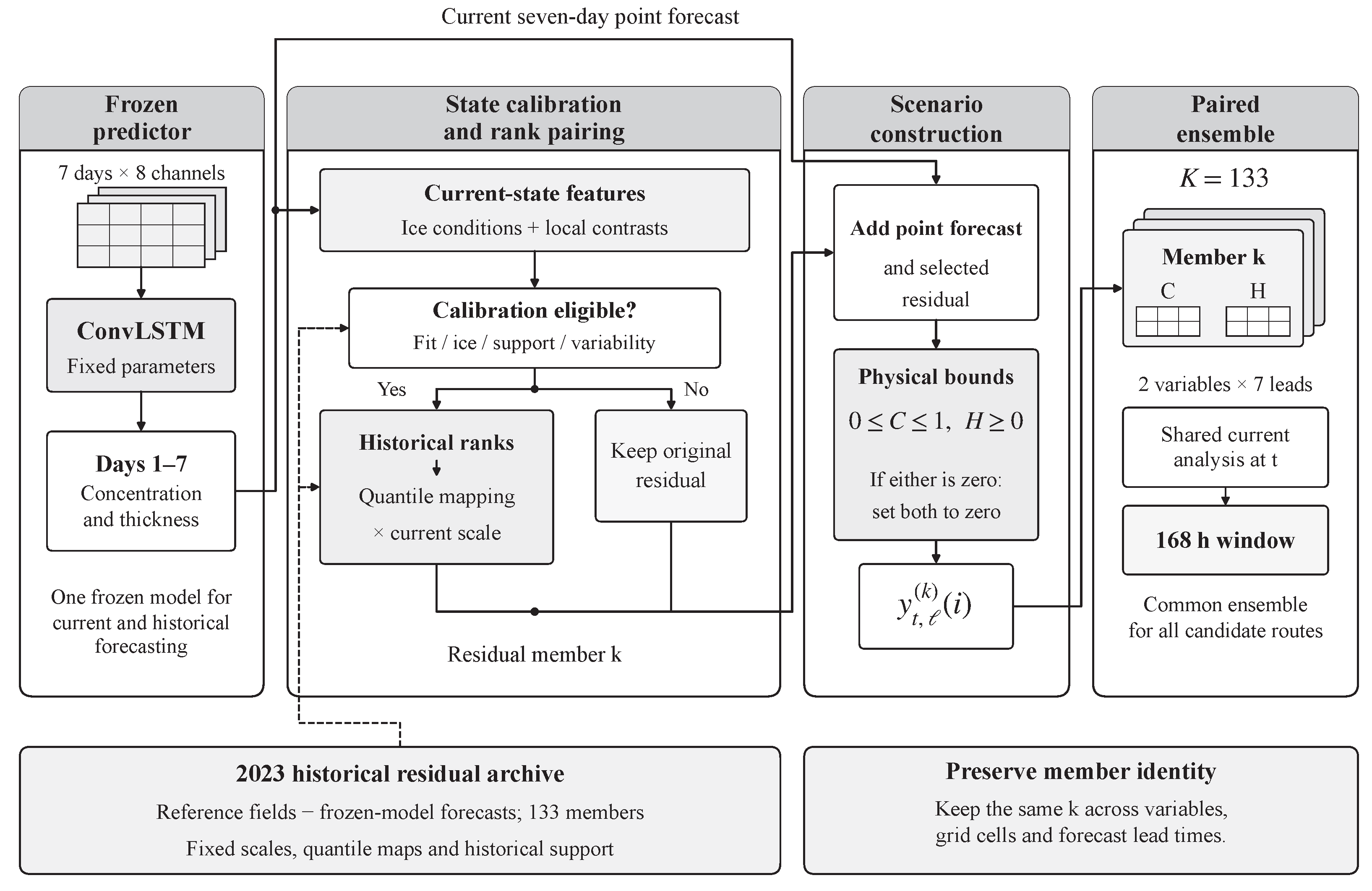
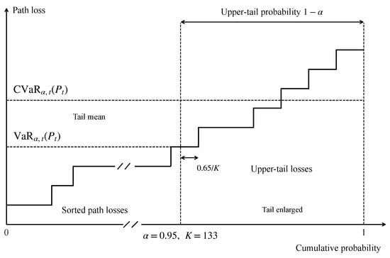
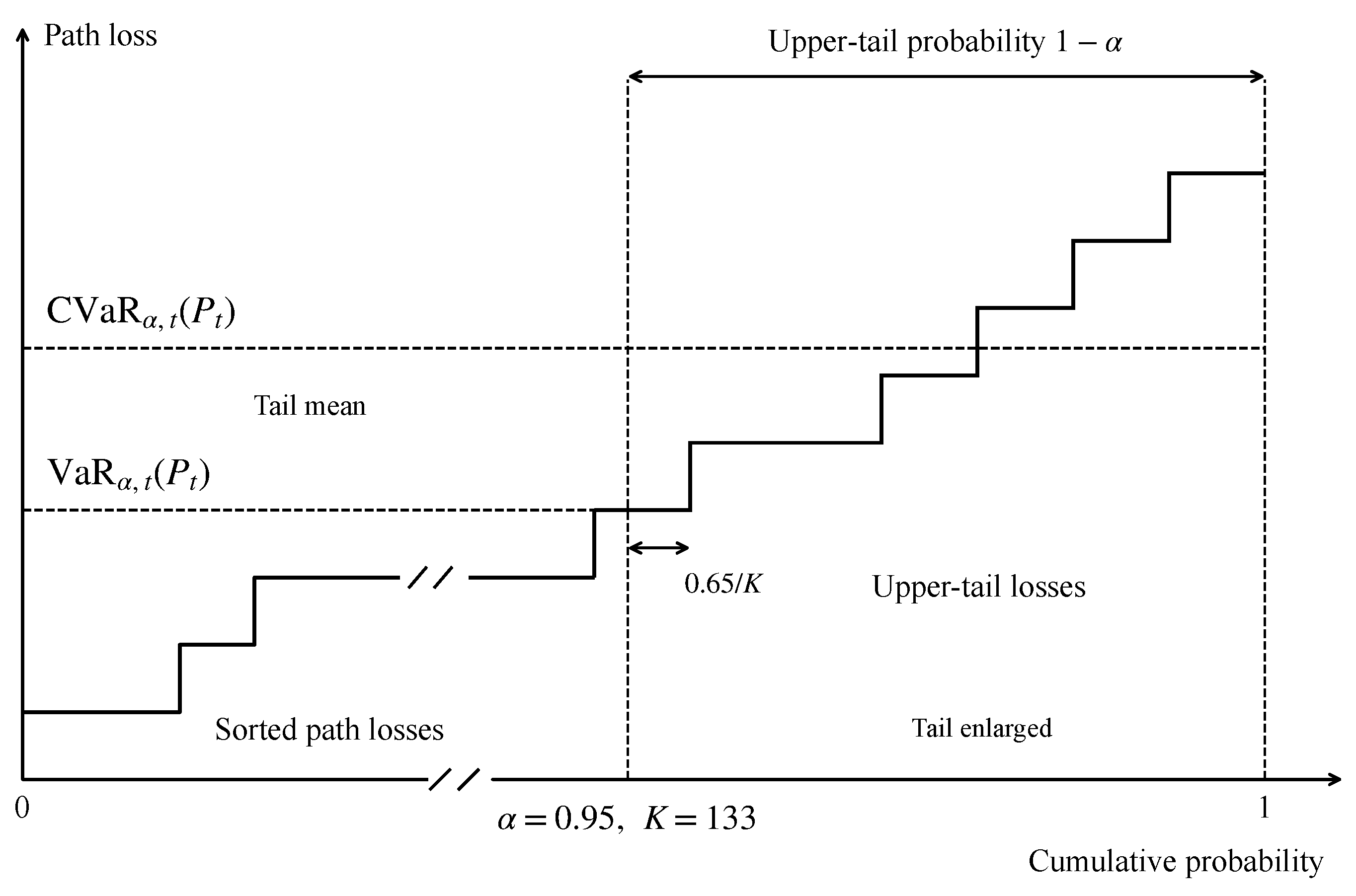
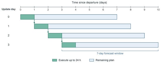
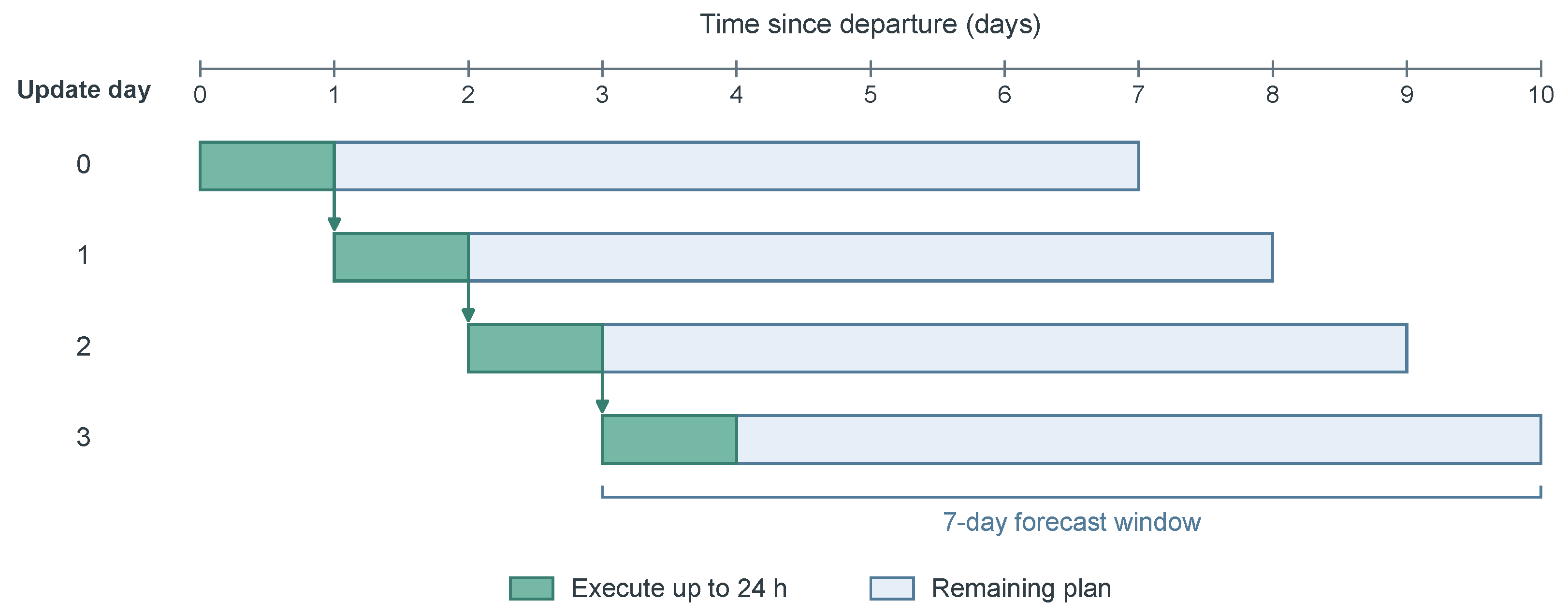
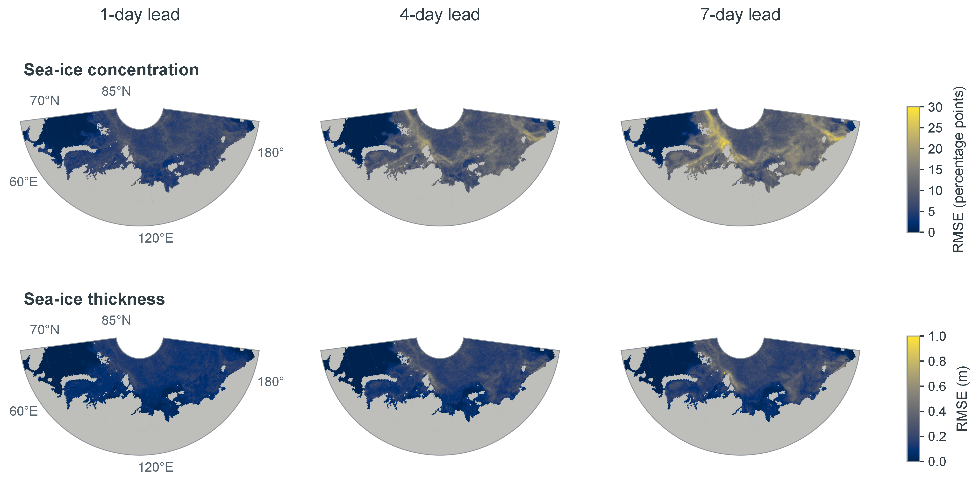
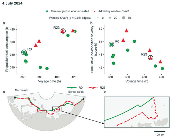
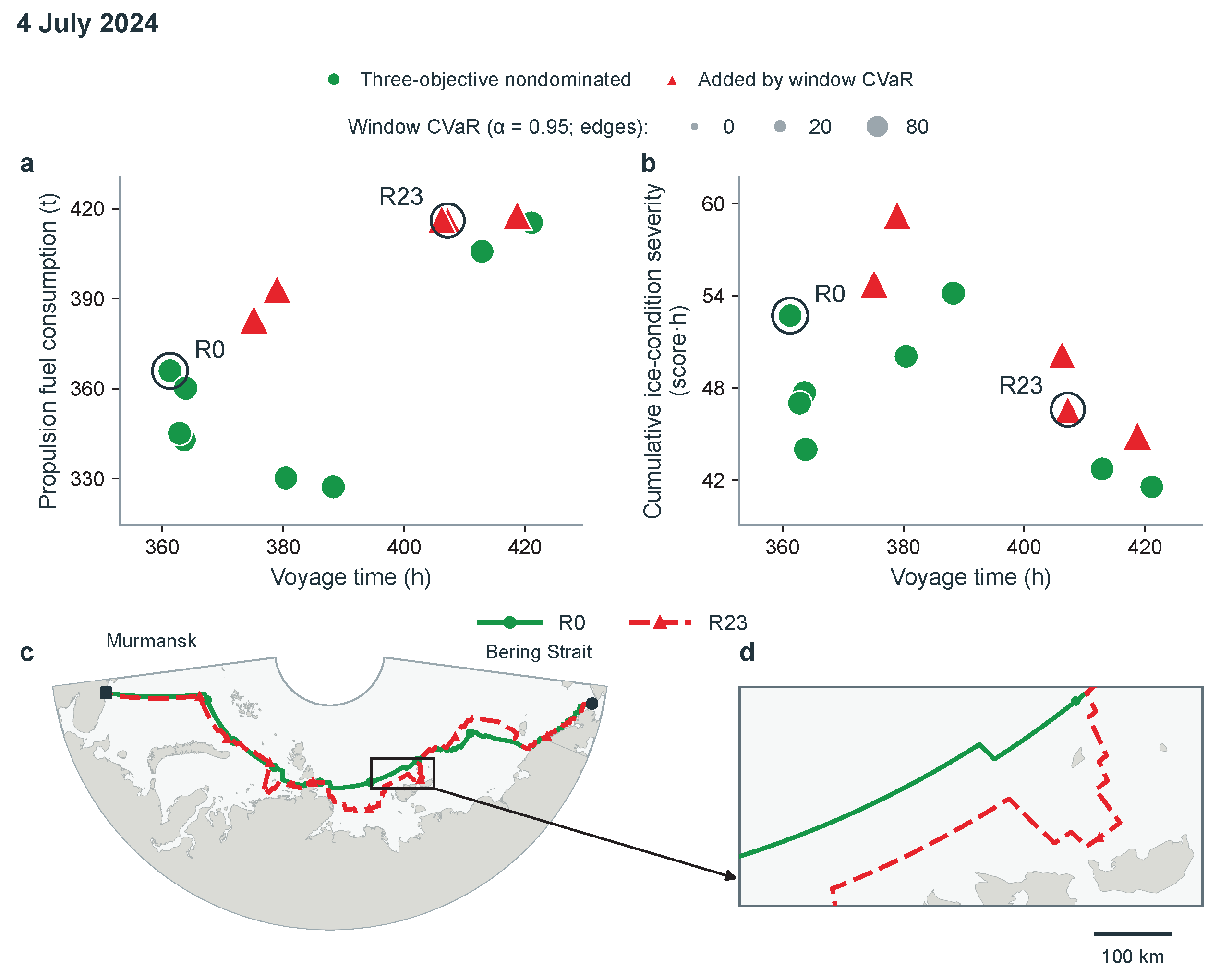
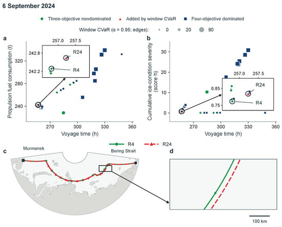
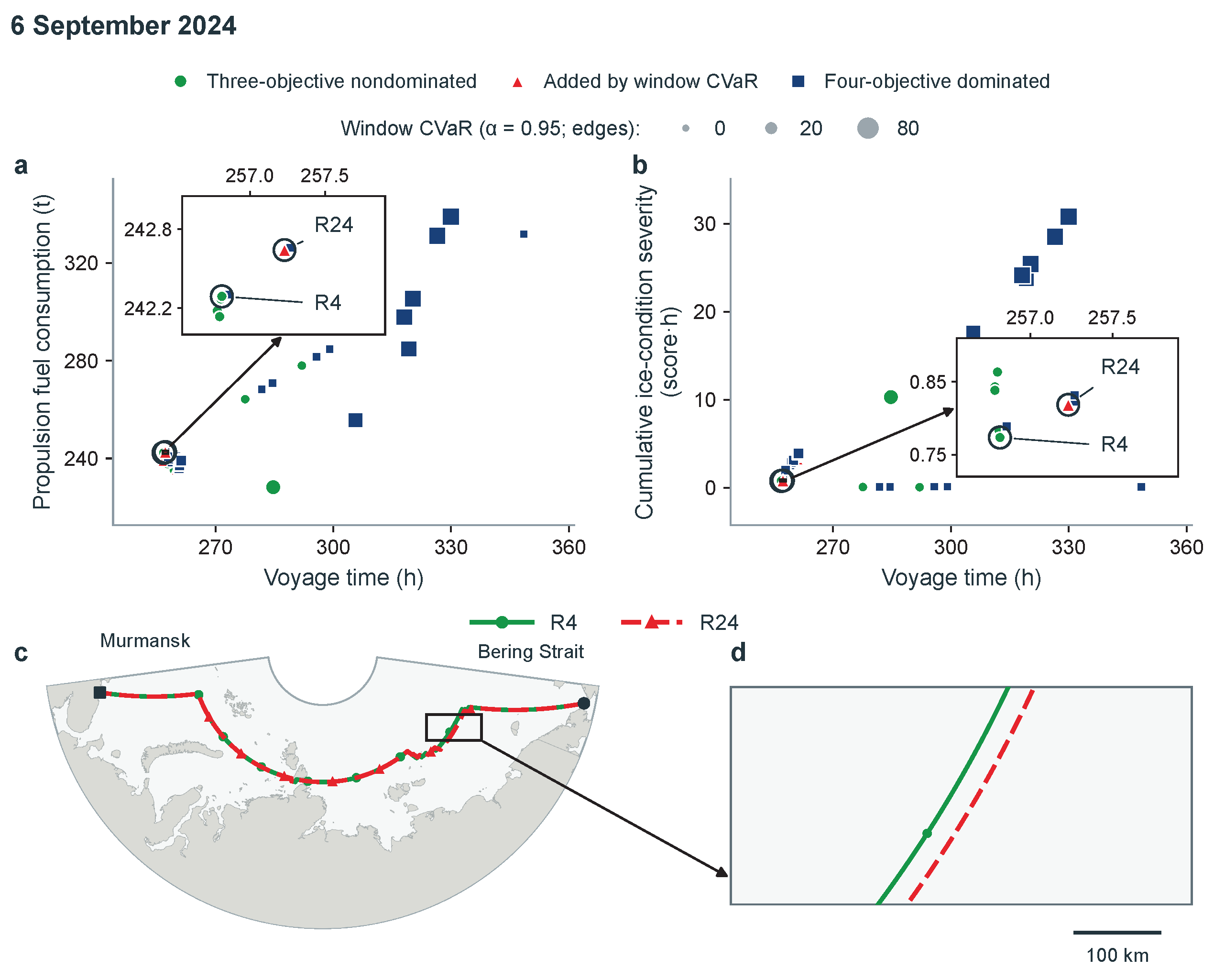
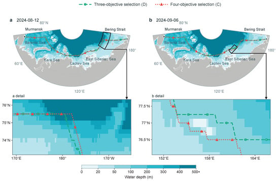
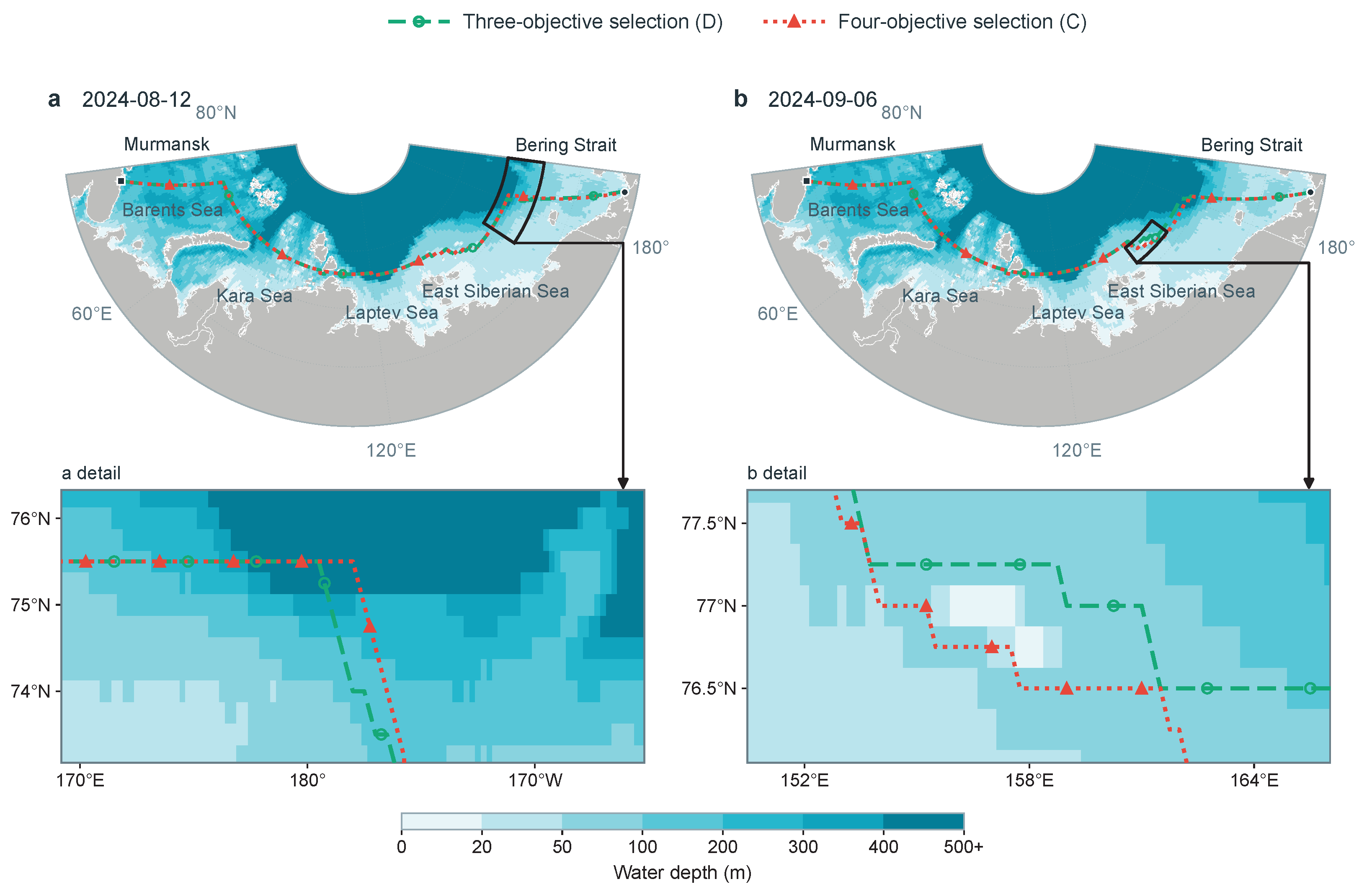
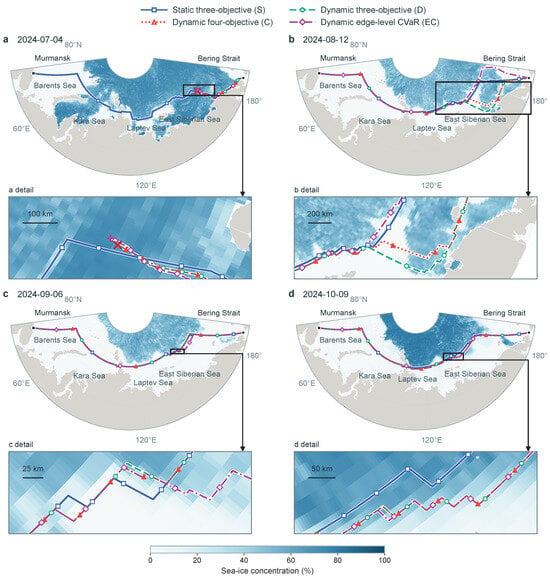
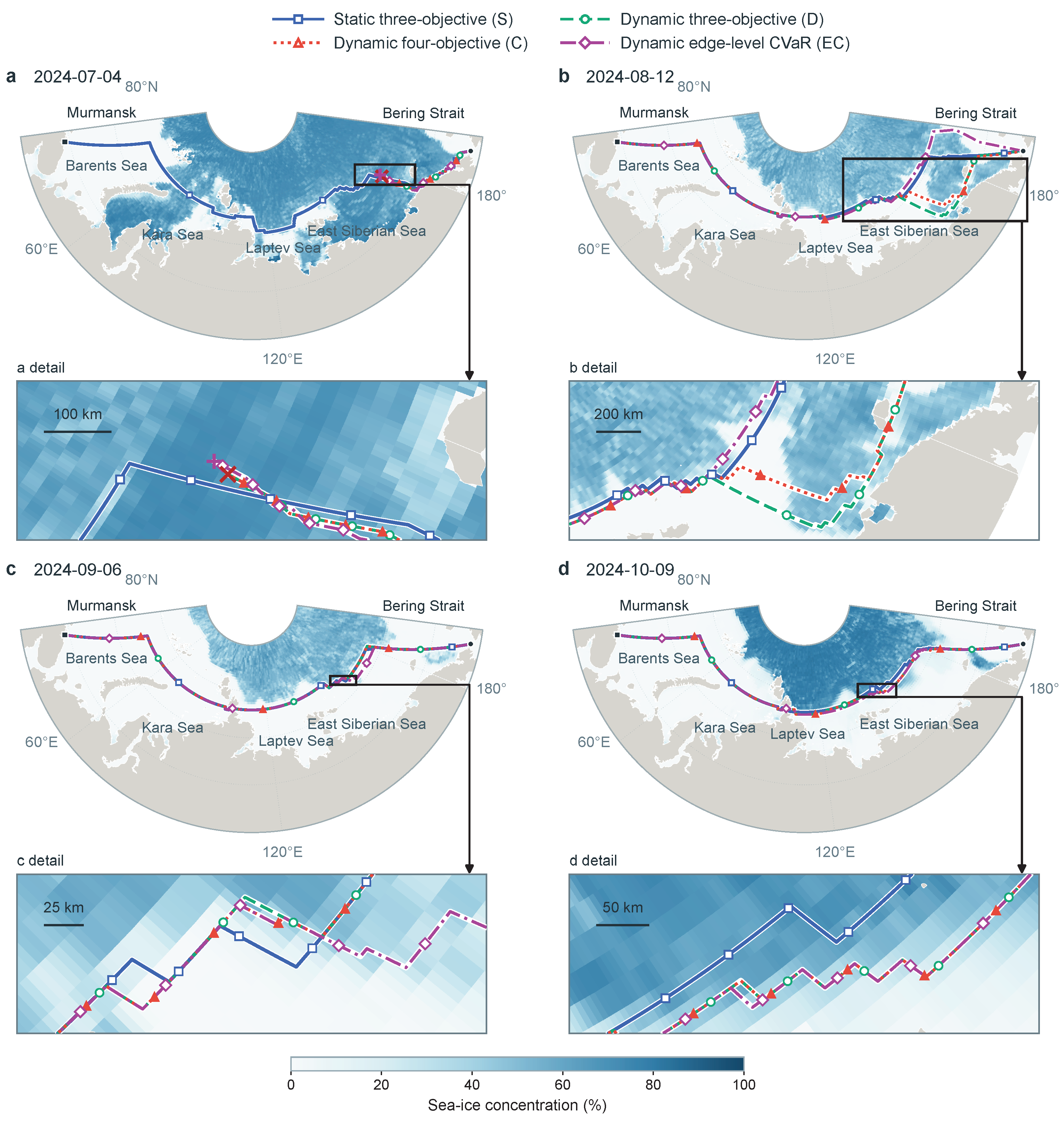
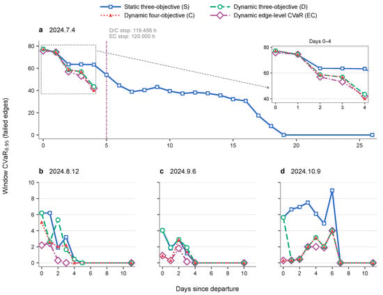
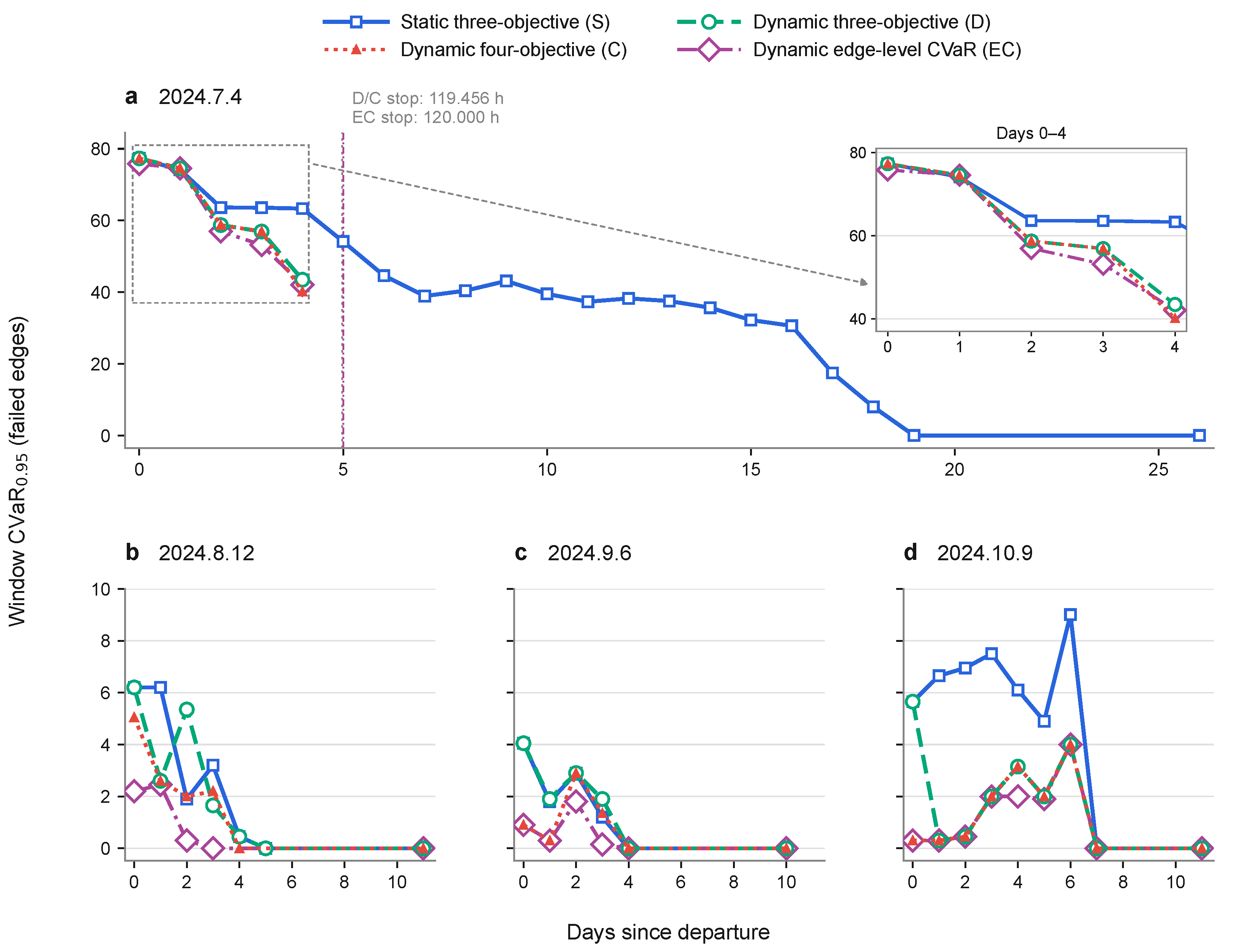
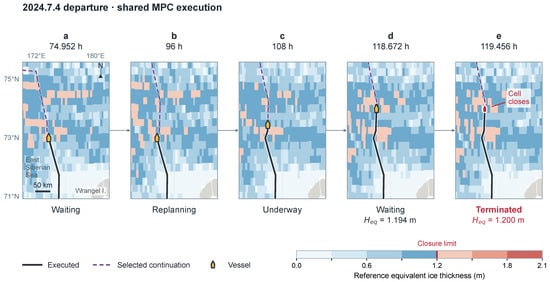
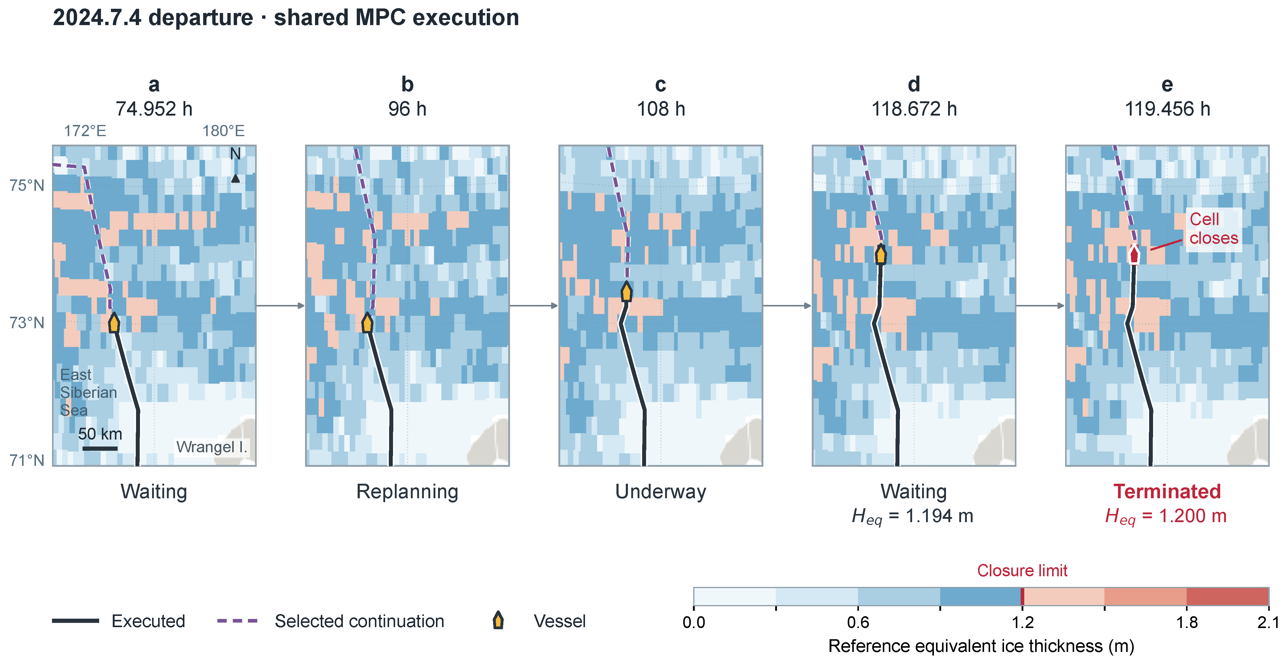
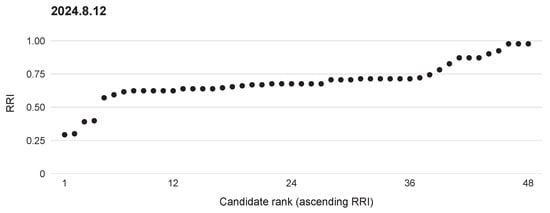
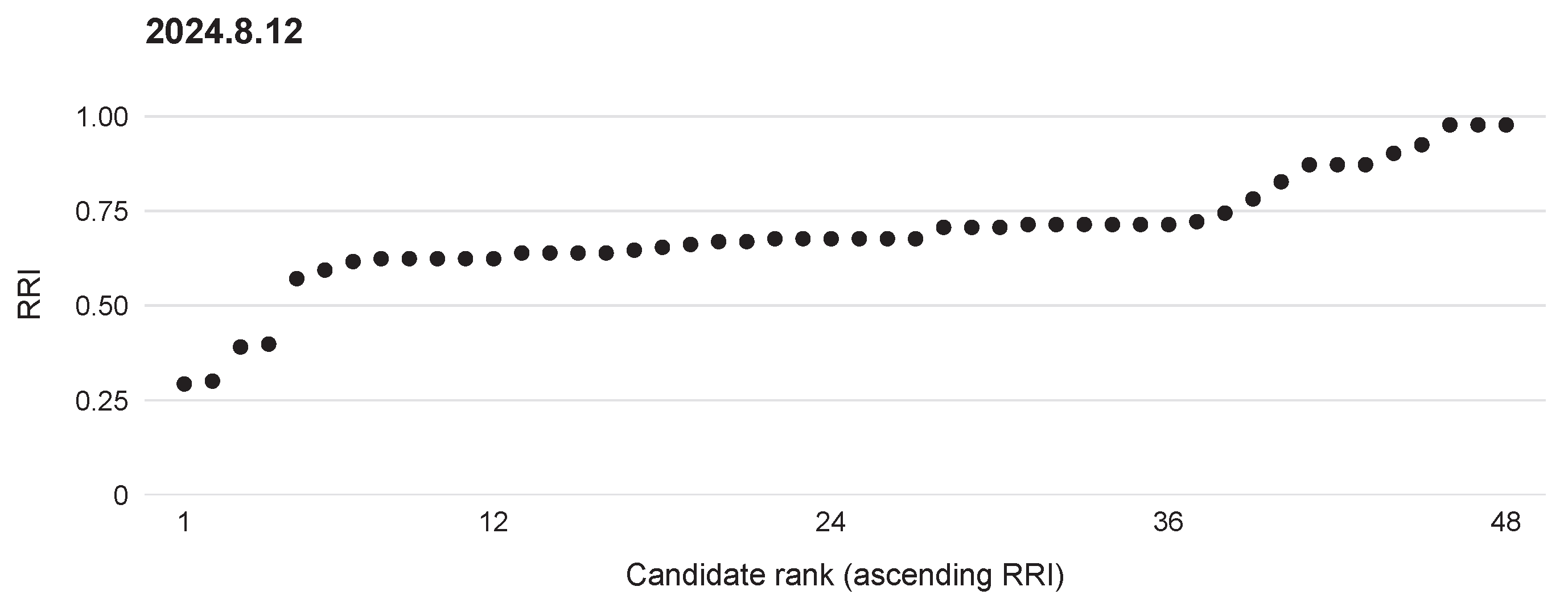
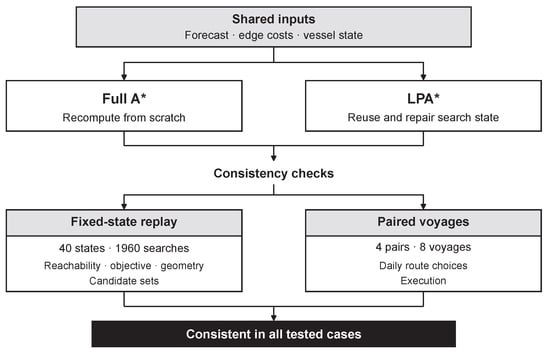
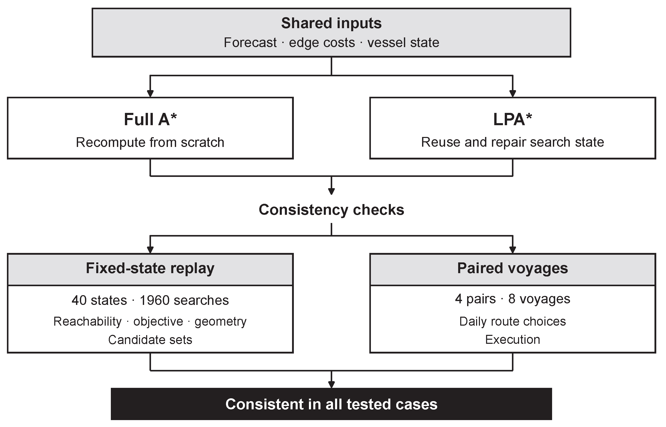
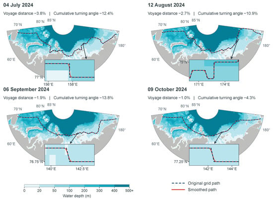
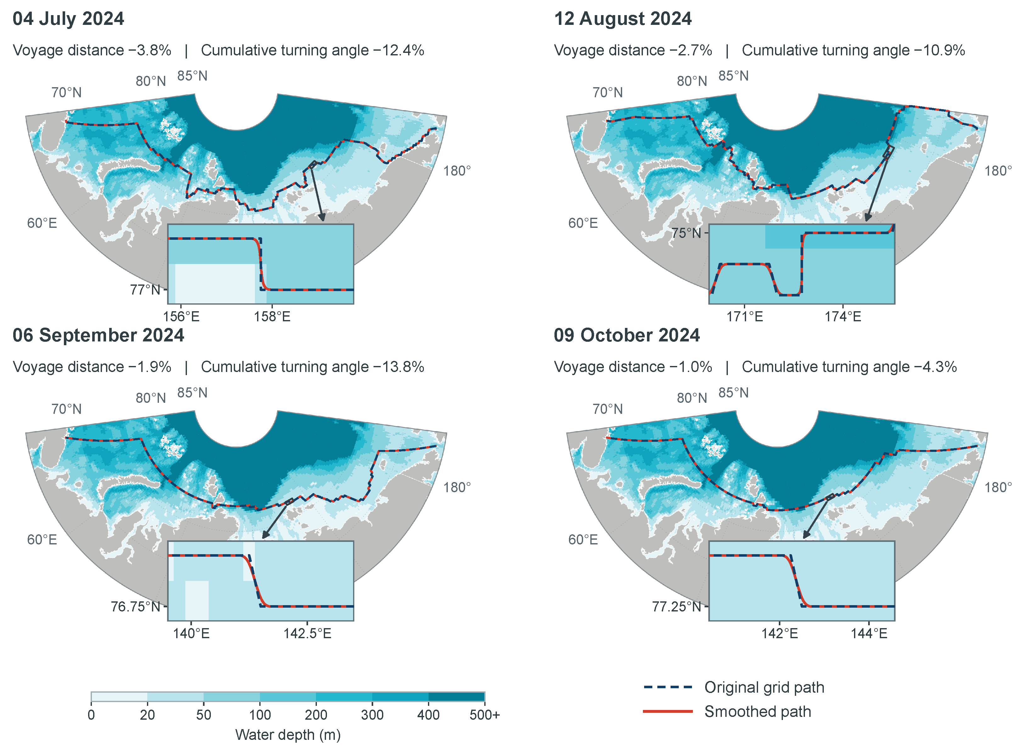

Disclaimer/Publisher’s Note: The statements, opinions and data contained in all publications are solely those of the individual author(s) and contributor(s) and not of MDPI and/or the editor(s). MDPI and/or the editor(s) disclaim responsibility for any injury to people or property resulting from any ideas, methods, instructions or products referred to in the content. |
© 2026 by the authors. Licensee MDPI, Basel, Switzerland. This article is an open access article distributed under the terms and conditions of the Creative Commons Attribution (CC BY) license.