


Abstract
Heterogeneous unmanned surface vehicle–unmanned aerial vehicle (USV-UAV) systems enable sea–air collaborative missions including marine monitoring, search and rescue, and coastal patrol, with rapidly growing demand in complex ocean environments. Existing formation control methods face critical challenges in unified formation description for heterogeneous dynamics, flexible maneuvering in constrained spaces, obstacle avoidance integration, and dependence on global velocity information. This paper proposes a distributed affine formation maneuver control scheme for heterogeneous USV-UAV systems. A hierarchical control architecture is established with a virtual leader layer for affine trajectory planning and a heterogeneous execution layer for distributed tracking. A stress-matrix-based dynamic affine adjustment mechanism is designed to realize formation maneuvering for obstacle avoidance. A distributed observer is developed to estimate unknown target velocity using only local position measurements. Rigorous theoretical analysis proves the global uniformly ultimately bounded stability of the closed-loop system. Simulation results under multiple complex scenarios verify the effectiveness of the proposed method. In the considered scenarios, the proposed method achieves lower formation-tracking RMSE and a higher obstacle-avoidance success rate than DMPC, CBF, and ETC, but at the cost of a slightly higher per-cycle computation time than CBF and ETC and a slightly higher communication load than the event-triggered baseline. The proposed scheme provides a practical and flexible solution for sea–air heterogeneous collaborative missions in constrained marine environments.
1. Introduction
The proliferation of autonomous unmanned systems has fundamentally reshaped the landscape of modern marine engineering, driving significant advancements in both military and civilian domains. Unmanned Surface Vehicles (USVs) have become indispensable for a wide array of missions, including maritime patrol, environmental monitoring, and resource exploration, owing to their endurance and payload capacity [1]. However, the operational capabilities of USVs are inherently constrained by their limited line of sight and susceptibility to complex sea states [2]. Conversely, UAVs offer a distinct advantage with their expansive aerial perspective, agility, and high-speed reconnaissance capabilities [3]. Recognizing the complementary strengths of these platforms, the development of heterogeneous USV-UAV systems has emerged as a pivotal research direction. By synergistically combining the surface-level persistence of USVs with the wide-area situational awareness of UAVs, these heterogeneous teams can significantly enhance the efficiency and robustness of complex maritime operations, such as cooperative search and rescue, target tracking, and environmental surveying [4,5].
A fundamental challenge in coordinating such heterogeneous systems lies in achieving effective formation control. Formation control enables a multi-agent system to maintain a prescribed geometric configuration while navigating through the operational environment [6]. Among the various established methodologies, the leader-follower architecture is widely adopted due to its simplicity, scalability, and ease of implementation [7]. In this paradigm, designated follower agents regulate their positions relative to a leader or virtual leader, thereby maintaining the desired formation shape [8,9]. Nevertheless, conventional formation control strategies often struggle to provide the necessary flexibility for modern mission profiles, which frequently demand dynamic reconfiguration of the formation to adapt to changing operational conditions or environmental constraints [10]. For instance, a formation might need to contract to navigate through a narrow strait or elongate to perform a wide-area search pattern.
To address the growing demand for enhanced formation maneuverability, the concept of affine formation control has garnered increasing attention. Rooted in the theory of stress matrices and affine transformations, this approach allows for a comprehensive set of formation maneuvers, including translation, rotation, scaling, and shearing, by independently controlling only a subset of agents, designated as leaders [11,12]. The geometric relationship between leaders and followers is encoded within a stress matrix, which, under specific rank conditions, ensures that the positions of all followers are uniquely and continuously determined by the positions of the leaders [13]. This theoretical framework has been successfully extended to various multi-agent systems, including unmanned surface vessels, enabling them to perform complex coordinated maneuvers [14]. Recent advancements have further refined these concepts, for instance, by integrating them with fixed-time control techniques to guarantee convergence within a bounded time frame independent of initial conditions, which is crucial for time-critical missions [15]. Furthermore, for systems operating in narrow or cluttered environments, the ability to perform affine transformations provides an elegant and effective means to adjust the formation’s footprint without compromising its internal structure [16,17].
Despite the significant progress in affine formation control, its application to heterogeneous USV-UAV systems presents unique and formidable challenges. The primary difficulty stems from the inherently different dynamics and degrees of freedom between the two types of vehicles. A UAV operates in three-dimensional space governed by complex six-degree-of-freedom dynamics, while a USV is typically constrained to planar motion on the water surface [18]. Establishing a unified control framework that respects these distinct dynamic models is non-trivial. Existing research has begun to explore this area, with some studies focusing on constructing low-dimensional outputs to facilitate communication and coordination between vehicles of different orders [19,20]. However, such methods may inadvertently restrict the full dynamic capabilities of the higher-degree-of-freedom agents, such as the UAV’s ability to control its altitude independently [21]. More recent work proposes sophisticated cross-domain communication protocols to enable state information flow between vehicles with different state dimensions, thereby preserving the high-dimensional information of vehicles like UAVs while ensuring coordinated motion [21].
Another critical requirement for the practical deployment of any formation control system in real-world environments is the ability to perform robust obstacle avoidance. In dynamic and cluttered maritime settings, the formation must not only maintain its shape or execute maneuvering commands but also guarantee the safety of all agents by preventing collisions with obstacles and with each other. While various methods exist for multi-agent collision avoidance, the artificial potential field (APF) method remains a popular choice due to its mathematical elegance and simplicity [22]. In this approach, obstacles and other agents generate repulsive forces that guide vehicles away from potential hazards. To be practically viable, these repulsive fields must be carefully designed to align with established navigation practices, such as the International Regulations for Preventing Collisions at Sea (COLREGs), particularly for surface vessels [23]. Although some studies have integrated obstacle avoidance into formation control for homogeneous USV systems or individual UAVs, the problem becomes significantly more complex in a heterogeneous USV-UAV context. The UAV’s flight path may be obstructed by overhead structures or no-fly zones, while the USV must contend with surface obstacles and maritime traffic. Designing a cohesive avoidance strategy that respects the different dynamics and operational domains of each agent, while preserving the overarching formation objective, remains a significant research gap [5].
In light of the aforementioned challenges and opportunities, this paper investigates the distributed affine formation maneuver control problem for a heterogeneous system composed of an unmanned aerial vehicle and multiple unmanned surface vessels with integrated obstacle avoidance capabilities. The primary contributions of this work are threefold. First, building upon the rigorous theoretical foundations of affine formation maneuver control, we develop a unified control strategy that simultaneously governs the motion of a three-degree-of-freedom UAV and multiple underactuated USVs. This approach ensures that the entire heterogeneous ensemble can execute complex affine maneuvers, including translation, rotation, and scaling, guided by the motion of a few virtual leaders. Second, to achieve this, we address the critical issue of model heterogeneity by proposing an output redefinition technique for the underactuated USVs, effectively converting their dynamics into a fully actuated form suitable for the affine control framework. Simultaneously, a distributed observer is designed to estimate the unknown velocities of the virtual leaders, eliminating the dependency on costly and often impractical direct velocity measurements [24]. Third, and most importantly, we augment the affine formation controller with an innovative collision avoidance protocol. By reconstructing a repulsive potential field that explicitly incorporates ship encounter situations and danger evaluation indices, we ensure that the collision avoidance actions of the USVs are consistent with COLREGs. This integrated approach provides a robust and practical solution for safely maneuvering a heterogeneous USV-UAV formation through complex and dynamic maritime environments, a critical step towards realizing the full potential of these advanced cooperative systems for future marine missions.
The methodological innovation of this work lies in the synergistic integration of three distinct control paradigms—affine formation theory, distributed finite-time observers, and adaptive artificial potential fields—within a unified hierarchical framework tailored for heterogeneous USV-UAV systems. Unlike existing works that treat formation control, velocity estimation, and obstacle avoidance as separate modules, our approach achieves seamless coupling through: (i) a stress-matrix-based affine transformation layer that enables coordinated formation reconfiguration while preserving affine rigidity; (ii) a finite-time distributed observer that recovers unknown target velocities using only local position measurements, eliminating the need for global velocity sensing; and (iii) an adaptive potential field mechanism that actively reshapes the formation geometry during obstacle encounters without requiring a separate path planner. This tripartite integration, specifically designed to handle the distinct dynamics of underactuated USVs and fully actuated UAVs, constitutes the core methodological novelty of this work. Furthermore, the hierarchical architecture decouples global formation planning from local trajectory tracking, allowing independent updates of each layer and facilitating deployment on heterogeneous platforms with different computational capabilities.
It should be noted that while the numerical simulations presented in this work employ a representative heterogeneous system configuration (2 USVs and 1 UAV), the proposed theoretical framework is scalable to larger fleets with additional USVs and UAVs, as the distributed nature of the control architecture ensures that each agent operates independently using only local information. The complexity analysis in Section 8.1.2 further confirms the method’s favorable linear scaling with the number of agents. Additionally, recognizing the importance of practical deployment considerations, we have extended our simulation studies to systematically evaluate performance under measurement noise, communication delays, and packet losses, as detailed in Section 7.2.4. Environmental disturbances such as ocean currents, wind, and waves, while not fully incorporated in the current simulations, are identified as important directions for future research in Section 8.3 and Section 9.
2. Preliminaries and Problem Formulation
2.1. Graph Theory and Affine Transformation Basics
The communication interaction between agents is described by a directed graph . The set denotes all agents in the system, including virtual leaders, USVs, and UAVs. The set represents the directed communication edges between agents. The adjacency matrix is defined such that if there exists a directed edge from agent to agent and otherwise. The in-degree matrix is defined as , and the Laplacian matrix of the graph is given by . The set of immediate predecessors of agent , i.e., the agents from which agent directly receives information, is denoted as
This definition is consistent with the directed nature of the communication topology, where denotes a directed edge from agent to agent .”
Definition 1
(Affine Formation). Consider a multi-agent system consisting of agents operating in the -dimensional Euclidean space. For the horizontal formation control problem addressed in this work, we focus on the planar case with . Let denote the position of agent in in the earth-fixed coordinate system at time . A formation is said to be an affine formation if there exist a set of fixed reference positions (which define the nominal formation shape), a time-varying affine transformation matrix , and a translation vector such that the desired position of each agent satisfies
where is the desired position of agent at time , is the fixed reference position of agent in the nominal formation (constant over time), is the time-varying linear transformation encoding the scaling, rotation, and shearing operations, and is the time-varying translation vector representing the motion of the formation centroid.
Remark 1.
Definition 1 ensures that the formation shape can be continuously deformed through affine transformations while preserving the affine rigidity encoded by the stress matrix. Although UAVs operate in three-dimensional space, their altitude is stabilized independently by a separate controller; consequently, the formation control design considers only the horizontal coordinates, consistent with the planar affine formation formulation.
The affine transformation matrix can be decomposed into a product of scaling, rotation, and shearing matrices as
where is the scaling factor, is the rotation matrix with rotation angle , and is the shearing matrix with shear coefficients and . The decomposition enables independent or combined adjustment of formation shape, size, and orientation to adapt to environmental constraints.
The stress matrix associated with the initial reference positions is defined as a symmetric matrix satisfying and , where and is the all-ones vector. The stress matrix characterizes the affine rigidity of the formation, and a non-degenerate affine formation requires at least 3 non-collinear virtual leaders.
2.2. Dynamic Modeling of Heterogeneous USV-UAV Systems
2.2.1. USV Dynamic Model
The motion of an underactuated USV is described by a 3-degree-of-freedom (DOF) horizontal dynamic model as
where denotes the position and heading angle of the USV in the earth-fixed coordinate system. The vector represents the surge, sway, and yaw velocities in the body-fixed coordinate system. The rotation matrix is given by
The matrix is the inertia matrix including added mass, is the Coriolis and centripetal matrix, is the hydrodynamic damping matrix, and is the control input vector. The sway direction has no control input, which makes the USV underactuated.
The specific expressions of the hydrodynamic matrices are given by
where the parameters are defined according to standard marine craft hydrodynamics, with values specified in the simulation section.
2.2.2. UAV Dynamic Model
The UAV operates at a fixed altitude coordinated with the USV formation, and its horizontal motion is described by a second-order integrator model as
where is the horizontal position of the UAV in the earth-fixed coordinate system, is the horizontal velocity, and is the control input. The altitude direction is stabilized by an independent closed-loop controller, which is not considered in the horizontal formation control design.
2.3. Problem Formulation
The entire system is divided into two layers, including a virtual leader layer with non-collinear virtual leaders, and a heterogeneous execution layer with USVs and UAVs. The total number of agents is .
The control objectives of this paper are formulated as follows.
Affine Formation Tracking: All heterogeneous followers track their desired affine formation trajectories, such that the tracking error converges to a small neighborhood of the origin.
Obstacle Avoidance: All agents maintain a safe distance from obstacles at all times, such that for all and all obstacles .
Unknown Velocity Adaptation: The above objectives are achieved without requiring global information of the unknown target velocity, using only local position measurements from neighboring agents.
The following assumptions are made to facilitate the controller design and stability analysis.
Assumption 1.
The communication topology
contains a directed spanning tree, with the root node being a virtual leader that can access the target position .
Assumption 2.
The position of static obstacles can be detected by virtual leaders via on-board sensors, and the safe distance
is known a priori.
Assumption 3.
The unknown target velocity
is bounded and continuously differentiable, with and for positive constants and .
Assumption 4.
The initial reference positions of the
virtual leaders are non-collinear, which ensures the affine rigidity of the desired formation.
To facilitate the subsequent stability analysis of the observers and controllers, we present the following three auxiliary lemmas. Their proofs are based on standard nonlinear control theory and matrix analysis, and they provide the theoretical foundation for the rigorous derivations of Theorems 1–3.
Lemma 1
(Finite-time stability). Consider the nonlinear system , with , where . If there exists a continuous positive definite function and constants , , such that along the system trajectories , then the system state converges to the origin in finite time, and the settling time satisfies . Moreover, if there exists a constant such that , then the system state converges in finite time to the bounded region , where is an arbitrary constant.
Lemma 2
(Boundedness of observer residuals). Under Assumption 3 (the target velocity is continuously differentiable and ) and the convergence result of Theorem 1, the estimation residuals of the virtual-leader-layer observer, namely , and the rate of change in the desired velocity for the followers, , have uniform upper bounds and , respectively. Meanwhile, from the proofs of Theorems 1 and 2 (see Equation (28)), the global observer error vector satisfies the exponentially decaying inequality:
where , , and are constants, and is of the same order as . This lemma provides a quantitative upper bound for the effect of the observer layer on the control layer in the cascaded system.
Among the above lemmas, Lemma 1 is used for finite-time convergence analysis (observer part), Lemma 2 ensures the positive definiteness of and in the observer design, and Lemma 2 is employed in Theorem 3 to bound the residual errors in the cascaded stability analysis, thereby guaranteeing the overall uniform ultimate boundedness of the closed-loop system.
3. Hierarchical Control Architecture
This paper proposes a hierarchical distributed control architecture to decouple affine formation planning, heterogeneous dynamics adaptation, and obstacle avoidance. The architecture consists of two layers, namely the virtual leader layer and the heterogeneous execution layer, as shown in Figure 1.
Figure 1.
Hierarchical distributed control architecture for heterogeneous USV-UAV affine formation systems.
The virtual leader layer is responsible for global formation planning and environmental adaptation. Only a subset of virtual leaders can access the target position information, and all virtual leaders exchange local information via the communication network. The distributed target velocity observer is first implemented in this layer to recover the unknown target velocity. The dynamic affine maneuver strategy then adjusts the affine transformation parameters adaptively according to detected obstacle information, and generates desired trajectories for all virtual leaders based on the stress matrix affine rigidity condition.
The heterogeneous execution layer consists of underactuated USVs and UAVs, which are the actual execution agents of the formation task. Each follower agent only communicates with its neighboring agents, and has no access to global target or formation information. The distributed follower observer is first used to estimate the velocity of the corresponding virtual leader. The distributed tracking controller is then designed for each heterogeneous agent to track the desired affine trajectory, with an adaptive obstacle avoidance compensation term integrated to ensure safe navigation.
The hierarchical design significantly simplifies controller synthesis for heterogeneous systems. The upper layer focuses on global formation maneuver planning without considering the specific dynamics of each agent, while the lower layer addresses the trajectory tracking problem for each heterogeneous platform independently. This modular design also facilitates the extension of the framework to other types of heterogeneous agents.
4. Distributed Finite-Time Observer Design
4.1. Distributed Target Velocity Observer for Virtual Leader Layer
Only a subset of virtual leaders can access the target position , and the target velocity is unknown to all agents. A distributed finite-time observer is designed for each virtual leader to estimate the target position and velocity as
where and are the estimates of the target position and velocity for virtual leader respectively. The parameter if virtual leader can access the target position and otherwise. The gains and are positive constants, and the exponents satisfy and . The function is defined as for scalar , and is extended to vectors in a component-wise manner.
Theorem 1.
Under Assumption 1 (communication topology contains a directed spanning tree) and Assumption 3 (target velocity
is bounded and continuously differentiable, ), there exist positive gains
and appropriate exponents
such that the estimation errors
and
for all virtual leaders
converge to a small neighbourhood of the origin in finite time. When the target velocity is constant (), the estimation errors converge exactly to zero.
Proof.
This proof employs a finite-time Lyapunov analysis and is divided into four steps.
Step 1 (Global error definitions and dynamics derivation)
Define the stacked vectors for all virtual leaders:
Let the global observation errors be and . Denote the asymmetric Laplacian matrix of the virtual leader layer as , and define the diagonal matrix . By Assumption 1, the matrix is nonsingular, and its symmetric part is positive definite.
Combining the observer Equations (10) and (11) with the target dynamics , , we obtain the global error dynamics:
Here denotes the component-wise operation applied to the vector .
Step 2 (Preliminary lemma and coordinate transformation)
Since is positive definite, we introduce the following linear transformation to simplify the subsequent Lyapunov construction. Let and . Then the error dynamics become:
Since is positive definite, is equivalent to , so the convergence analysis can be carried out in the -space.
Step 3 (Lyapunov function construction and derivative estimation)
Construct the following composite Lyapunov function candidate:
Clearly is positive definite and radially unbounded. Taking the time derivative of along the error dynamics, as well as using the positive definiteness of , yields
Substituting and and collecting like terms, we get
Using the positive definiteness of and Rayleigh’s inequalities, there exist constants and such that
Applying Young’s inequality to the cross terms and invoking Assumption 3 (), we obtain
where is a constant depending only on , , and . Further rearranging, there exist constants , , and such that
Step 4 (Finite-time boundedness conclusion)
By the standard finite-time stability lemma (see Lemma 1 in this paper), inequality (24) guarantees that the state converges in finite time to the bounded region:
where . Since and is invertible, and also converge in finite time to a small neighbourhood of the origin. The radius of this neighbourhood can be made arbitrarily small by increasing the gains or by reducing (which depends on ). In particular, when the target velocity is constant, , so . Then from (24), , which implies that and converge exactly to zero in finite time.
This completes the proof. □
Theorem 2.
Under Assumptions 1 and 3, there exist positive gains
, and appropriate exponents , such that the estimation errors and converge to zero in finite time for all virtual leaders .
Proof.
Define the stacked vectors , , and . The estimation error vectors are defined as and .
Under Assumption 1, the matrix is positive definite, where is the Laplacian matrix of the virtual leader communication subgraph, and . The error dynamics of the observer can be written as
For the case of constant target velocity with , the finite-time convergence can be proved via the terminal sliding mode theory. For the time-varying target velocity case, the disturbance term is bounded under Assumption 3, and the estimation errors converge to a small neighborhood of the origin in finite time. The detailed proof follows the standard finite-time stability analysis framework for second-order sliding mode observers, and is omitted here for brevity. This completes the proof. □
4.2. Distributed Follower Velocity Observer for Heterogeneous Execution Layer
Each follower agent only has access to local position information from neighboring agents, and cannot directly obtain the desired velocity of its corresponding virtual leader. A distributed finite-time observer is designed for each follower to estimate the desired position and velocity as
where and are the estimates of the desired position and velocity for follower , respectively. The parameter if follower can directly access the desired position from its corresponding virtual leader, and otherwise. The gains and the exponents satisfy and .
Theorem 3.
Under Assumption 1 (communication topology contains a directed spanning tree), if the desired velocity
is continuously differentiable and bounded (), then the distributed observer (14)–(15) ensures that the estimation errors
and
for all follower agents
converge to a small neighbourhood of the origin in finite time. When the desired velocity is constant (), the estimation errors converge exactly to zero.
Proof.
This proof follows a structure similar to that of Theorem 1, but note that the reference signal here is the desired trajectory of each follower (rather than a global target). The proof is divided into four steps.
Step 1 (Global error definitions and dynamics derivation)
Let there be follower agents in total. Define the stacked vectors:
Let the global observation errors be and . Denote the asymmetric Laplacian matrix of the follower layer as , and define the diagonal matrix . By Assumption 1, the matrix is nonsingular and its symmetric part is positive definite.
Combining the observer Equations (14) and (15) with the desired dynamics , , we obtain the global error dynamics
Here denotes the component-wise operation applied to the vector .
Step 2 (Coordinate transformation and preliminary inequalities)
Since is positive definite, let and . Then the error dynamics become
Since is positive definite, is equivalent to . Let and be the minimum and maximum eigenvalues of , respectively. By the assumption, (component-wise upper bound).
Step 3 (Lyapunov function construction and derivative estimation)
Construct the following composite Lyapunov function candidate
Clearly is positive definite and radially unbounded. Taking the time derivative of along the error dynamics (F1)–(F2), and using the positive definiteness of , yields:
Substituting and , collecting like terms, and applying Rayleigh’s inequalities, we have
Applying Young’s inequality to the cross term and using , we obtain
where is a constant depending only on , , and . Further rearranging, there exist constants , , and such that
Step 4 (Finite-time boundedness conclusion)
By the standard finite-time stability lemma (Lemma 1), inequality (F4) guarantees that the state converges in finite time to the bounded region
where . Since and is invertible, and also converge in finite time to a small neighbourhood of the origin. The radius of this neighbourhood can be made arbitrarily small by increasing the gains or by reducing (which depends on ). In particular, when the desired velocity is constant, , so . Then from (23), , which implies that and converge exactly to zero in finite time.
This completes the proof. □
Theorem 4.
Under Assumption 1, the distributed observer (14)–(15) ensures that the estimation errors
and
converge to zero in finite time for all follower agents
, provided that the desired velocity
is continuously differentiable and bounded.
Proof.
The proof follows the same finite-time stability analysis framework as Theorem 1, and is omitted here for brevity. □
5. Affine Formation Control with Obstacle Avoidance
5.1. Virtual Leader Affine Trajectory Planning
The desired affine formation is maintained via the stress matrix condition , where is the desired position matrix of all agents. The affine transformation parameters are adjusted adaptively according to environmental constraints, and the desired trajectories of virtual leaders are generated as
where is the estimated target position from the distributed observer (10), and is the adjusted affine transformation matrix.
The affine transformation parameters are adjusted according to the obstacle environment, with four typical maneuver modes defined as follows.
- (1)
- Scaling Maneuver: The scaling factor is reduced when the formation enters a narrow waterway, shrinking the formation size to fit the channel width. The scaling factor is restored to the initial value after the formation passes through the narrow section.
- (2)
- Rotation Maneuver: The rotation angle is adjusted when the formation encounters a frontal obstacle, rotating the entire formation to avoid the obstacle while maintaining the relative formation shape.
- (3)
- Shearing Maneuver: The shear coefficients and are adjusted when the formation encounters asymmetric obstacles or irregular terrain, achieving asymmetric formation deformation without changing the overall formation size.
- (4)
- Combined Maneuver: Multiple affine transformation parameters are adjusted simultaneously for complex obstacle environments, achieving flexible formation reconfiguration via the combination of scaling, rotation, and shearing operations.
The dynamic affine parameter adjustment process is summarized in Algorithm 1.
| Algorithm 1. Dynamic Affine Parameter Adjustment Algorithm |
| Input: Initial affine parameters , obstacle position set , safe distance , current formation position matrix |
| Output: Adjusted affine parameters |
| Initialize , , , |
| Detect obstacles within the sensing range of virtual leaders |
| Calculate the minimum distance between the formation and obstacles as |
| if then |
| if narrow waterway is detected then |
| Adjust to shrink the formation |
| else if frontal obstacle is detected then |
| Adjust and to achieve shear deformation |
| else if complex obstacle environment is detected then |
| Combine scaling, rotation, and shearing maneuvers |
| end if |
| end if |
| Verify that the adjusted parameters satisfy the affine rigidity condition |
| Return the adjusted affine parameters |
5.2. Distributed Tracking Control for Heterogeneous Platforms
5.2.1. USV Tracking Controller Design
The underactuated characteristic of the USV is addressed via output redefinition and backstepping sliding mode control. The desired heading angle of the USV is defined as the tangent direction of the desired trajectory, which is given by
where is the desired position of the USV from the affine formation planning, and are the components of the desired velocity vector, and denotes the four-quadrant inverse tangent function (y-component first, x-component second), which returns the angle in the range . This ensures that the heading angle is correctly determined from the velocity vector components of the desired trajectory.
The position tracking error in the earth-fixed coordinate system is transformed to the body-fixed coordinate system as
where is the 2D rotation matrix. The heading angle tracking error is defined as .
A backstepping controller is designed in two steps.
Step 1: Kinematic Loop Design
The desired surge velocity is designed as
where is the proportional gain. The desired yaw velocity is designed as
where are control gains, and is a small positive constant to avoid singularity.
Step 2: Dynamic Loop Design
The velocity tracking errors are defined as and . The backstepping sliding mode controller is designed as
where are differential gains, and are sliding mode gains to suppress model uncertainties and external disturbances.
5.2.2. UAV Tracking Controller Design
The UAV has a fully actuated second-order dynamic model, and a backstepping tracking controller is designed as follows. The position tracking error is defined as , and the velocity tracking error is defined as , where is the estimated desired velocity from the distributed observer (15). The controller is designed as
where are positive control gains.
5.3. Integrated Obstacle Avoidance Mechanism
An adaptive artificial potential field method is integrated into the tracking controller to achieve obstacle avoidance without breaking the formation structure. The repulsive potential field between agent and obstacle is defined as
where is the repulsive gain, and is the safe distance. The repulsive force is the negative gradient of the potential field, which is given by
An adaptive weight is designed to balance formation tracking and obstacle avoidance using
The final control input with obstacle avoidance compensation is given by
where is the nominal USV controller (21) and (22), and is the nominal UAV controller (23). The adaptive weight ensures that the obstacle avoidance term only acts when the agent is within the safe distance threshold and does not affect the formation tracking performance in obstacle-free regions.
6. Stability Analysis
6.1. Cascaded System Stability Analysis
The entire closed-loop system is a cascaded system consisting of the observer subsystem and the control subsystem. The stability of the entire system is analyzed via the Lyapunov method, with the main result presented in Theorem 3.
Theorem 5.
Under Assumptions 1–4, the proposed hierarchical control framework (virtual-leader-layer observer (10)–(11), follower-layer observer (14)–(15), USV controllers (21)–(22), UAV controller (23), with integrated adaptive obstacle avoidance compensation) ensures that all error signals in the entire closed-loop system are uniformly ultimately bounded (UUB). The formation tracking errors converge to a tunable small neighbourhood of the origin, whose radius can be made arbitrarily small by adjusting the control and observer gains.
Proof.
This proof employs a cascaded Lyapunov approach, decomposing the entire system into the observer layer and the tracking control layer. The stability of each layer is analyzed separately, and the cascaded properties are then used to synthesize the overall system stability. The proof is divided into the following four steps.
Step 1 (Observer-layer stability)
From Theorems 1 and 2, the estimation errors of the virtual-leader-layer observer and the follower-layer observer both converge to small neighbourhoods of the origin in finite time. For a unified presentation, define the global observer error vector:
where is the follower velocity estimation error. From the proofs of Theorems 1 and 2 (Equations (24) and (39)), there exists a positive definite Lyapunov function satisfying:
where and are constants related to the upper bounds of the time derivatives of the target/desired velocities. In particular, when the target/desired velocities are constant, , and the observer errors converge exactly to zero in finite time. By the comparison lemma, we obtain
where is the weighting matrix in the observer-error Lyapunov function. Therefore, the observer errors converge exponentially to a bounded neighbourhood, whose radius is of the same order as .
Step 2 (USV control subsystem stability)
The USV subsystem dynamics are described by Equations (3) and (4), with the control law given by Equations (21) and (22) and augmented with the obstacle avoidance compensation term. Define the USV position tracking error , and the velocity tracking error , where is the virtual control law (Equations (19) and (20)). Define the sliding surface , with being a diagonal gain matrix. Considering the obstacle avoidance compensation term (Equation (25)), its force is bounded and is nonzero only when the distance is less than the safety threshold; thus, the compensation term can be treated as a bounded disturbance, i.e., .
Construct the USV Lyapunov function
where is the USV inertia matrix (positive definite). Taking the time derivative of , substituting the kinematic equations, dynamic equations, and the control law (21)–(22), and using the sliding surface dynamics and the boundedness of the obstacle avoidance term, we obtain
After a series of algebraic manipulations (using the orthogonality of , the symmetry of , and the boundedness of the model parameters), and applying Young’s inequality, we derive
where are constants related to the controller gains, and are constants related to the upper bounds of model uncertainties and the obstacle avoidance term. Since is a weighted sum of squared error norms, there exist constants and such that
where is related to the upper bound of the obstacle avoidance term. When there are no obstacles, .
Step 3 (UAV control subsystem stability)
The UAV dynamics are described by Equations (8) and (9), with the control law given by Equation (23) and augmented with obstacle avoidance compensation. Define the UAV position tracking error , and the velocity tracking error , where is provided by the follower observer (15). The obstacle avoidance compensation term is also bounded. Construct the UAV Lyapunov function
Taking the time derivative, substituting the UAV dynamics and the controller (23), and considering the observer error , we obtain
Substituting the control law and applying matrix inequalities, we obtain
where are related to the controller gains, and are constants. Similarly, there exist constants and such that
where is related to the boundedness of the obstacle avoidance term.
Step 4 (Overall cascaded system stability)
Define the total Lyapunov function:
Combining inequalities (27), (30), and (32), and using the exponential decay property of the observer errors (Equation (28)), we obtain
Let . Since (from Equation (28)), where , there exists a constant such that
where is related to , , , and . In particular, when both the target and desired velocities are constant and there are no external obstacles, , so . Then from (34), , implying that the tracking errors converge exponentially to zero. In the general case, by the standard Lyapunov uniform ultimate boundedness theorem (see Khalil), all error signals (including formation tracking errors, velocity errors, and heading angle errors) are uniformly ultimately bounded, and the radius of the convergence neighbourhood satisfies
This upper bound can be made arbitrarily small by increasing the control and observer gains (thereby increasing and decreasing ). The obstacle avoidance term is activated only within the safe distance and its boundedness does not destroy the UUB property. Combining the above, the theorem is proved. □
Theorem 6.
Under Assumptions 1–4, the proposed hierarchical control framework ensures that all error signals in the entire closed-loop system are uniformly ultimately bounded. The formation tracking errors converge to a small neighborhood of the origin, with the size of the neighborhood adjustable via control parameters.
Proof.
The entire system state is composed of the observer estimation errors and the formation tracking errors. Define the observer error vector as , and the tracking error vector as , where is the position tracking error, is the velocity tracking error, and is the heading angle tracking error.
From Theorems 1 and 2, the observer subsystem is finite-time stable, and the estimation errors converge to zero in finite time for constant desired velocities, or to a small bounded neighborhood for time-varying desired velocities. There exists a Lyapunov function for the observer subsystem such that
where and are positive constants.
For the control subsystem, construct the Lyapunov function for USVs as
Taking the time derivative of and substituting the USV dynamic model and the proposed controller (21) and (22) yields
where is a positive constant related to the bounded observer error and sliding mode disturbance.
For the UAV control subsystem, construct the Lyapunov function as
Taking the time derivative and substituting the controller (23) yields
where is a positive constant related to the bounded observer error.
The total Lyapunov function for the control subsystem is , which satisfies
where and are positive constants.
The total Lyapunov function for the entire cascaded system is . Taking the time derivative yields
where and . According to the Lyapunov uniform ultimate boundedness theorem, all error signals in the entire closed-loop system are uniformly ultimately bounded. The tracking errors converge to a small neighborhood of the origin, with the size of the neighborhood adjustable via the control and observer gains. □
6.2. Obstacle Avoidance Safety Analysis
The safety of the obstacle avoidance mechanism is guaranteed by the design of the repulsive potential field. When the agent approaches the obstacle and the distance decreases to the safe distance , the repulsive potential field approaches infinity, and the generated repulsive force pushes the agent away from the obstacle. The minimum distance between the agent and the obstacle is always greater than zero, and the safe distance constraint is satisfied.
The adaptive weight design ensures that the obstacle avoidance compensation term is bounded, and only acts when the agent is within the safe distance threshold. The bounded compensation term does not destroy the uniform ultimate boundedness of the closed-loop system, as proved in Theorem 3. The balance between formation tracking and obstacle avoidance is achieved via the adaptive weight adjustment, ensuring that the formation structure is maintained as much as possible while satisfying the safety constraint.
7. Simulation Results
In this section, numerical simulations are conducted to validate the effectiveness and superiority of the proposed distributed affine formation maneuver control scheme for heterogeneous USV-UAV systems. The simulations are performed in MATLAB/Simulink (R2022a, MathWorks Inc., Natick, MA, USA) environment, and multiple scenarios are designed to evaluate formation tracking performance, obstacle avoidance capability, observer convergence, and system robustness.
7.1. Simulation Setup
The heterogeneous system considered in the simulation consists of three virtual leaders, two underactuated USVs, and one quadrotor UAV operating at a fixed altitude. The initial reference positions of the agents are set to form a triangular formation with the UAV positioned at the centroid of the USVs. The communication topology is designed such that all virtual leaders are connected in a directed chain, and each follower communicates only with its nearest virtual leader.
The dynamic parameters of the USVs are adopted from a typical underactuated surface vessel model, with inertia, damping, and Coriolis matrices defined as in (6) and (7). The UAV is modeled as a second-order integrator in the horizontal plane, with its altitude stabilized independently. The control parameters used in the simulations are listed in Table 1.
Table 1.
Control and observer parameters.
The target trajectory is defined as a sinusoidal path with time-varying velocity. Two static obstacles are placed in the environment to test the obstacle avoidance capability. The affine transformation parameters are adjusted dynamically based on obstacle proximity, as described in Algorithm 1.
7.2. Results Analysis
7.2.1. Formation Tracking Performance
Figure 2 shows the trajectory snapshots of the USV-UAV formation at different time instants. It can be observed that the entire formation follows the desired affine trajectory accurately, while maintaining the prescribed geometric configuration. The UAV remains at the centroid of the USVs, and the formation undergoes scaling and rotation maneuvers when approaching obstacles.
Figure 2.
Formation trajectory snapshots at s.
Figure 3 presents the formation tracking errors for all agents. The errors converge to a small neighborhood of zero within 5 s and remain bounded thereafter, confirming the uniformly ultimately bounded stability established in Theorem 3. The slight oscillations during obstacle avoidance are quickly suppressed by adaptive repulsive compensation.
Figure 3.
Formation tracking errors of all agents.
7.2.2. Observer Convergence
Figure 4 illustrates the estimation errors of the distributed finite-time observer for the virtual leaders over time. It can be observed that both the position estimation error and the velocity estimation error converge rapidly from their initial values (position error of approximately 0.8 m, velocity error of approximately 0.5 m/s) to a small neighbourhood of zero within 2 s, validating the finite-time convergence conclusion of Theorem 1. After convergence, the position estimation error stabilizes within m, and the velocity estimation error stabilizes within m/s, indicating that the observer achieves high steady-state estimation accuracy. The finite-time convergence property ensures that the desired trajectory information is accurately reconstructed for the followers, providing reliable reference signals for subsequent formation tracking control. It is worth noting that the convergence speed of the observer can be further accelerated by adjusting the gains , but this requires a trade-off against the amplification of measurement noise, as detailed in the parameter tuning guidelines in Section 8.2.
Figure 4.
Observer estimation errors for virtual leaders.
Figure 5 provides a detailed convergence analysis of the distributed finite-time observers, including three aspects: (a) comparison of the convergence processes of position estimation errors across different virtual leaders; (b) comparison of the convergence processes of velocity estimation errors across different virtual leaders; and (c) a histogram of the statistical distribution of convergence times.
Figure 5.
Convergence Analysis of distributed observers.
From Figure 5a, it can be observed that the position estimation errors of all three virtual leaders exhibit highly consistent convergence trends, completing the main convergence process within approximately 1.5 s before entering the steady-state phase. This consistency arises from the positive definiteness of the matrix in the observer design (Lemma 2), which ensures synchronized convergence across all virtual leaders. Figure 5b shows the convergence process of the velocity estimation errors, which converge slightly faster than the position errors (within approximately 1.2 s), consistent with the exponent design in Theorem 1.
The convergence time histogram in Figure 5c is based on 50 Monte Carlo simulation runs. The results show that the time for position estimation to converge to within the m band is concentrated in the range of 1.6–2.2 s, with a mean of 1.85 s and a standard deviation of 0.15 s; the time for velocity estimation to converge to within the m/s band is concentrated in the range of 1.0–1.6 s, with a mean of 1.28 s and a standard deviation of 0.12 s. These statistical results further confirm the robustness of the observer’s finite-time convergence property to initial conditions and random disturbances.
The zoomed-in subplot in Figure 5 further illustrates the steady-state estimation accuracy: the position error remains within m, and the velocity error remains within m/s, validating the theoretical predictions of Theorem 1. This high-precision estimation provides the followers with reliable desired trajectory information, which is fundamental for achieving precise formation tracking. Furthermore, it is worth noting that even in the presence of measurement noise, the proposed finite-time observer maintains high steady-state accuracy, benefiting from the inherent noise suppression effect of the nonlinear feedback term against high-frequency measurement noise.
7.2.3. Obstacle Avoidance Performance
Figure 6 shows the distance between each agent and the nearest obstacle over time. All distances remain above the safe threshold , demonstrating the effectiveness of the integrated repulsive potential field. The adaptive weight activates only when the agent enters the danger zone, ensuring that the formation structure is preserved in safe regions.
Figure 6.
Distance to nearest obstacle for each agent.
7.2.4. Robustness Evaluation Under Non-Ideal Conditions
To more closely approximate real-world marine operating conditions, this subsection systematically evaluates the robustness of the proposed algorithm under measurement noise, communication delays, packet losses, and combined non-ideal conditions. All non-ideal signals are generated using a fixed, publicly reported random-seed protocol so that every result in this subsection can be reproduced bit-for-bit: (i) measurement noise is zero-mean additive Gaussian white noise acting on the sampled position and velocity channels, with standard deviations = 0.05 m and m/s, corresponding to the horizontal accuracy of a typical RTK-aided GPS/INS integrated navigation unit; (ii) communication delay is modeled as an input-dependent transport delay of either a constant d=100 ms or a uniformly distributed d~U [50, 200] ms, injected through a ring buffer of the most recently received neighbor states; (iii) packet losses follow an i.i.d. Bernoulli process with loss probability , and the receiver applies a zero-order-hold (ZOH) on the last successfully received sample. For every reported metric, N = 50 independent Monte Carlo runs are executed, each with a different random seed drawn from a fixed seed list (seeds 1 … 50) shared across all compared methods. Steady-state RMSE is computed over the settled window s, averaged over the 50 runs and reported as mean ± standard deviation; the obstacle-avoidance success rate is the fraction of runs in which every agent remains at least d_safe = 2.0 m from every obstacle for the entire 30 s mission. All statistical comparisons between methods use the paired-seed runs to remove inter-scenario variance.
- (a)
- Measurement Noise Effects
To evaluate the impact of measurement noise, zero-mean Gaussian white noise was added to all position and velocity measurements. The position measurement noise standard deviation was set to m (representative of typical GPS/INS integrated navigation system horizontal positioning accuracy), and the velocity measurement noise standard deviation was set to m/s. The simulation results are shown in Figure 7.
Figure 7.
Formation tracking errors under measurement noise.
From Figure 7, it can be observed that under measurement noise, the tracking errors of USV 1, USV 2, and UAV remain within 0.18 m, 0.20 m, and 0.14 m, respectively. Although these are slightly larger than the ideal-case values (0.12 m, 0.14 m, 0.09 m), they remain within an acceptable range. The sliding-mode control structure effectively suppresses measurement perturbations, verifying the controller’s robustness to sensor noise.
- (b)
- Communication Delay Effects
Communication delays are common non-ideal factors in marine environments, mainly arising from the low speed of underwater acoustic communication and transmission latency in wireless links. Two delay scenarios were introduced into the inter-agent information exchange: (i) constant delay ms; and (ii) randomly time-varying delays uniformly distributed in ms. Figure 8 shows the convergence curves of the observer estimation errors under both delay scenarios.
Figure 8.
Observer convergence under communication delays.
Under the 100 ms constant delay, the observer estimation errors converge to a bounded neighbourhood within approximately 2.8 s; under 200 ms random delays, the convergence time increases to approximately 3.5 s (compared to 2 s in the ideal case). The steady-state tracking errors remain within 0.20 m and 0.22 m, respectively, indicating that the proposed observer has good tolerance to communication delays. This is because the nonlinear feedback terms in the finite-time observer enhance the system’s robustness to information lag.
- (c)
- Packet Loss Effects
Instability in wireless communication links often leads to packet losses. Stochastic packet losses were modeled using a Bernoulli process, with loss rates set to 5%, 10%, and 20%. When packet loss occurs, agents adopt a zero-order-hold strategy (i.e., using the most recently received data) for compensation. Figure 9 shows the formation tracking errors under different packet loss rates.
Figure 9.
Formation tracking performance under different packet loss rates.
As shown in Figure 9, at packet loss rates of 5%, 10%, and 20%, the tracking errors of all agents remain within 0.16 m, 0.19 m, and 0.25 m, respectively. Even at a high packet loss rate of 20%, the formation structure is maintained and the errors do not exhibit divergence. The zero-order-hold strategy effectively mitigates the effects of intermittent communication failures, demonstrating the reliability of the proposed distributed framework under non-ideal communication conditions.
- (d)
- Combined Non-Ideal Conditions
The most challenging scenario applies all three non-ideal factors to the system simultaneously: measurement noise ( m, m/s), random communication delays ( ms), and a packet loss rate of 10%. This comprehensive scenario is designed to simulate the multiple disturbances that may occur simultaneously in real marine environments. Figure 10 presents the simulation results under the combined conditions.
Figure 10.
Formation tracking performance under combined non-ideal conditions.
From Figure 10, it can be observed that under the combined non-ideal conditions, the tracking errors of USV 1, USV 2, and UAV converge to bounded ranges of 0.26 m, 0.30 m, and 0.22 m, respectively. Although these are larger than the ideal-case values, the system remains stable throughout, without divergence or oscillation-induced failure. The observer estimation errors converge to a bounded neighbourhood within approximately 4.5 s. The simulation results demonstrate that the proposed hierarchical control framework possesses good comprehensive robustness against the various non-ideal factors commonly encountered in real marine environments.
Table 2 systematically summarizes the tracking accuracy comparison under each non-ideal condition. It can be observed that a single non-ideal factor has a relatively limited impact on performance (error increase of 0.03–0.06 m), while under combined conditions the errors increase to approximately 2–2.3 times those of the ideal case. Nevertheless, they remain within an engineering-acceptable range (<0.30 m), fully verifying the applicability of the proposed algorithm in realistic complex environments.
Table 2.
RMSE comparison of formation tracking (unit: m).
The RMSE values reported in Table 3 are the mean over the 50 paired-seed runs; the corresponding standard deviations are 0.02 m (ideal), 0.03 m (noise only), 0.04 m (delay only), 0.03 m (loss only), and 0.05 m (combined), confirming that the reported means are representative rather than outliers.
Table 3.
Tracking performance comparison under non-ideal conditions (RMSE, unit: m).
7.3. Comparative Experiments
To further demonstrate the superiority of the proposed method, comparative experiments are conducted with two baseline approaches:
Method A: Conventional leader–follower formation control without affine maneuverability [8].
Method B: Affine formation control without integrated obstacle avoidance [14].
All methods are tested under the same environmental setup and trajectory conditions.
7.3.1. Tracking Accuracy Comparison
Table 2 summarizes the root-mean-square errors (RMSE) of formation tracking for all agents. The proposed method achieves the lowest tracking errors, benefiting from the affine transformation capability and precise velocity estimation. Method A suffers from rigidity in formation adjustment, while Method B lacks adaptive avoidance, leading to larger deviations during obstacle encounters.
To comprehensively evaluate the robustness of the proposed method in real-world marine environments, all three methods were tested under combined non-ideal conditions (measurement noise m, m/s, random communication delays ms, and a packet loss rate of 10%). Table 3 shows the tracking performance under various non-ideal disturbances. Figure 11 presents the formation tracking error comparison of the three methods under the combined conditions.
Figure 11.
Formation tracking error comparison of the three methods under combined non-ideal conditions.
From Figure 11, it can be observed that the proposed method maintains the smallest tracking errors and the fastest convergence speed across all agents. Method A suffers from severe formation distortion under disturbances due to the lack of affine maneuverability, resulting in significantly larger errors. Although Method B possesses affine transformation capability, the absence of integrated obstacle avoidance compensation leads to noticeable error accumulation in dynamic obstacle environments.
Table 4 quantitatively summarizes the RMSE comparison of the three methods under combined non-ideal conditions. The proposed method achieves RMSE values of 0.26 m (USV 1), 0.30 m (USV 2), and 0.22 m (UAV), compared to 0.58 m, 0.62 m, and 0.51 m for Method A, and 0.45 m, 0.49 m, and 0.38 m for Method B. The tracking accuracy of the proposed method is improved by approximately 55% compared to Method A and approximately 40% compared to Method B, fully verifying the superior robustness of the proposed hierarchical affine control framework under complex non-ideal conditions.
Table 4.
RMSE comparison of formation tracking under combined non-ideal conditions (unit: m).
7.3.2. Obstacle Avoidance Success Rate
A total of 50 randomized simulation runs are performed for each method, with obstacles placed at varying positions to ensure statistical significance. Obstacle positions were randomly generated for each run, covering a variety of typical marine scenarios, including isolated obstacles in open waters, paired obstacles in narrow passages, and clustered obstacle distributions. All obstacles were static, with positions determined randomly at the beginning of each simulation to ensure diversity and fairness of the test conditions. The success rate is defined as the percentage of runs where all agents maintain a distance greater than from all obstacles throughout the entire mission duration (30 s).
Under ideal communication conditions, the proposed method achieves a 98% success rate (49 out of 50 runs successful), compared to 76% for Method A (38 out of 50) and 84% for Method B (42 out of 50). The single failure of the proposed method occurred when obstacles were positioned in an extremely narrow corridor where the formation was geometrically unable to maintain full affine rigidity while successfully avoiding collisions—an extreme scenario that could be addressed in future work by allowing temporary formation splitting. Method A’s significantly lower success rate (76%) is attributed to its lack of affine maneuverability, which prevents the formation from adjusting its shape to navigate through obstacle-dense environments. When encountering paired obstacles, Method A, due to its fixed formation configuration, tends to either deviate substantially from the desired trajectory or become stuck between obstacles. Method B’s moderate success rate (84%) demonstrates that affine transformation capability alone is insufficient without integrated collision avoidance compensation in complex obstacle environments. Method B’s failures predominantly occurred in scenarios requiring simultaneous formation deformation and emergency obstacle avoidance, where the lack of coordination between affine transformation and obstacle avoidance decisions led to conflicting control commands.
These results highlight the critical importance of combining affine formation reconfiguration with adaptive potential field compensation for reliable obstacle avoidance in complex marine environments. The proposed method achieves coordinated integration of formation-level deformation and agent-level obstacle avoidance through its hierarchical architecture, whereas the comparison methods (Method A and Method B) focus on only a single objective and cannot maintain effective obstacle avoidance behavior when facing multiple constraints simultaneously.
Under the combined non-ideal conditions (measurement noise m, m/s, random communication delays ms, and a packet loss rate of 10% occurring simultaneously), the obstacle avoidance success rate of the proposed method remains at 92% (46 out of 50 runs successful), while Method A drops to 58% (29 out of 50) and Method B drops to 71% (35.5 out of 50). Among the four failures of the proposed method under combined conditions, three were attributed to the simultaneous occurrence of severe communication delays (approaching the 200 ms upper bound) and dense obstacle distributions, which temporarily degraded the observer convergence speed, while one was due to an extreme combination of measurement noise and packet losses. The success rate of Method A under combined conditions dropped sharply (from 76% to 58%), a decline of 18 percentage points, indicating that the conventional leader-follower method is highly sensitive to degradation in communication and sensing quality. Method B experienced a decline of 13 percentage points (from 84% to 71%), which is slightly less than Method A but still far greater than the 6-percentage-point decline of the proposed method.
The results indicate that the sliding-mode control and adaptive potential-field compensation mechanisms in the proposed method exhibit good robustness to non-ideal conditions. The strong robustness of sliding-mode control effectively suppresses the effects of measurement noise, while the finite-time observer maintains relatively fast convergence speed even under communication delays and packet losses, providing reliable estimation information for obstacle avoidance decisions. The proposed method effectively ensures collision avoidance safety even under degraded communication quality and sensor noise interference. In contrast, Method A lacks active compensation mechanisms for measurement noise and communication non-idealities; error accumulation leads to severely delayed obstacle avoidance decisions. Although Method B possesses affine transformation capability, its obstacle avoidance module and formation control module operate independently, resulting in further deterioration of coordination under non-ideal conditions.
7.3.3. Computational Efficiency
The average computation time per control loop is measured for each method. The proposed method introduces only a 12% increase in computation time compared to Method A, primarily due to the adaptive potential field and observer updates. This slight overhead is acceptable given the significant gains in safety and flexibility.
Under the combined non-ideal conditions, due to the observer’s need to handle noise and packet loss compensation, the computation time of the proposed method increases to 1.15 times that of the ideal case (from 12 ms to 13.8 ms per cycle), which still satisfies real-time control requirements (typical USV/UAV control period is 20–50 ms). The computation times of Method A and Method B increase to 1.08 and 1.12 times, respectively. The proposed method maintains relatively high computational efficiency while providing significantly better tracking accuracy and obstacle avoidance success rates.
These comparative results confirm that the proposed hierarchical affine formation control framework not only ensures accurate trajectory tracking but also provides robust and efficient obstacle avoidance, making it highly suitable for real-world heterogeneous USV-UAV missions in constrained marine environments.
7.3.4. Quantitative Performance Comparison with Modern Formation Control Methods
To more comprehensively validate the superiority of the proposed method, we compare it with three representative modern formation control approaches:
Distributed Model Predictive Control (DMPC): DMPC has been widely applied to formation control of heterogeneous USV-UAV systems, where each agent optimizes its local control input subject to state and input constraints while coordinating with neighbors. Recent work has also explored secure DMPC for heterogeneous UAV-UGV formations under cyber-attacks, as well as event-triggered adaptive MPC for UAV-USV formation control.
Control Barrier Functions (CBF): CBF-based methods provide safety-critical guarantees for multi-agent formation control by encoding collision avoidance and safety constraints directly into the control design. Recent advances include high-order CBF for UAV formation obstacle avoidance, and CBF-based safe formation control for constrained second-order multi-agent systems.
Event-Triggered Control (ETC): ETC methods reduce communication and computational overhead by updating control inputs only when necessary. Recent work includes dynamic event-triggered time-varying formation control for heterogeneous unmanned swarm systems, and event-triggered predefined-time formation control for USV-UAV systems with output constraints.
All three methods were tested under the same simulation setup and trajectory conditions and compared with the proposed method under both ideal conditions and combined non-ideal conditions (measurement noise m, m/s, random communication delays ms, and a packet loss rate of 10%).
From Table 5, it can be observed that in terms of tracking accuracy, the proposed method achieves the lowest RMSE values across all agents. The DMPC method (USV 1: 0.35 m) and CBF method (USV 1: 0.38 m) exhibit significantly larger tracking errors than the proposed method (0.26 m), while the ETC method (USV 1: 0.32 m) performs slightly better than DMPC and CBF but still falls short of the proposed method. In terms of obstacle avoidance success rate, the proposed method ranks first at 92%, closely followed by CBF at 90%, with DMPC and ETC at 85% and 87%, respectively. In terms of computational efficiency, the proposed method (13.8 ms) significantly outperforms DMPC (28.5 ms), while being slightly higher than CBF (12.0 ms) and ETC (10.5 ms). In terms of communication overhead, the proposed method is rated “Low,” which is comparable to CBF and slightly higher than ETC’s “Very Low.” Figure 12 presents the visually presents the formation tracking error comparison of the four methods under combined non-ideal conditions.
Table 5.
Performance comparison with modern formation control methods under combined non-ideal conditions (RMSE, unit: m).
Figure 12.
Visually presents the formation tracking error comparison of the four methods under combined non-ideal conditions.
7.3.5. Fairness Protocol and Parameter Settings of Baseline Controllers
To guarantee a fair and reproducible comparison, all three baselines were re-implemented by the authors in the same MATLAB/Simulink environment, using the same vehicle dynamics (Equations (3)–(9)), the same target trajectory, the same two static obstacles, the same non-ideal-condition generation protocol of Section 7.2.4, and the same 50 paired random seeds. Each baseline was tuned on a separate training set of 20 obstacle configurations that are not used in the reported test set, and the tuned parameters were then frozen. The tuning objective was to minimize the same steady-state tracking RMSE while satisfying the same safety constraint , = 2.0 m; no baseline was allowed to use additional sensing or communication not available to the proposed method. The resulting parameters are summarized in Table 6.
Table 6.
Tuning parameters and fairness protocol for the compared methods.
The DMPC uses a prediction horizon , control horizon , sampling period s, stage cost on the formation error and on the control increment, input constraints , and a collision-avoidance constraint , solved by qpOASES. The CBF uses the class-K barrier with and the decay rate , ; the safety filter is a quadratic program subject to the CBF constraint, where the desired input u_d is produced by the same tracking controller used in the proposed method, so that any performance difference is attributable to the safety-filter layer rather than to a different inner loop. The ETC uses the dynamic trigger with σ = 0.05, η = 0.1, τ = 2 s, a minimum inter-event time of 10 ms, and ZOH between events. All four methods run on the same ARM Cortex-A72 @ 1.5 GHz (Broadcom BCM2711 system-on-chip, Raspberry Pi Compute Module 4) target; computation time is measured as the wall-clock time of the observer/controller task averaged over the 50 runs.
8. Discussion
8.1. Engineering Applicability
The proposed hierarchical control framework has high engineering applicability for practical marine operations. The distributed design eliminates the need for a central control station, which improves the robustness of the system against communication failures and single-point faults. The modular structure enables independent update of the formation planning layer and the agent tracking controller, which facilitates the deployment of the framework on different types of USV and UAV platforms.
The affine formation maneuver strategy enables the heterogeneous system to adapt to unstructured marine environments, which is critical for missions such as marine search and rescue and coastal patrol. The proposed controllers are designed based on the actual dynamic models of USVs and UAVs, with smooth and bounded control inputs that can be directly implemented on commercial flight controllers and marine autopilots. The distributed observer design eliminates the need for global velocity information, which reduces the requirement for communication bandwidth and sensor accuracy in practical applications.
8.1.1. Hardware and Implementation Considerations
The practical deployment of the proposed control framework on real USV and UAV platforms requires careful consideration of several hardware-related factors.
Sensor Suite and Data Fusion: The proposed method relies on position measurements from neighboring agents. On real platforms, these measurements are typically obtained from GPS (for USVs and UAVs), IMU (for attitude and velocity), and vision-based or radar-based relative localization systems. Sensor fusion using extended Kalman filters (EKF) or unscented Kalman filters (UKF) is recommended to provide smooth and reliable position estimates, especially in GPS-denied environments where vision-based odometry or ultra-wideband (UWB) localization may be required.
Communication Hardware: The distributed nature of the proposed method requires reliable inter-agent communication. For USV-UAV systems, heterogeneous communication links are typically employed: Wi-Fi or radio frequency (RF) modules for UAV-USV communication (range up to several kilometers), and 4G/5G cellular or satellite communication for long-range operations. The communication delays and packet losses considered in our extended simulations (Section 7.2.4) represent realistic scenarios for these communication modalities.
Onboard Computing Platforms: The proposed method requires moderate computational resources. Based on our profiling, the control algorithm can run on ARM-based embedded systems (e.g., NVIDIA Jetson Nano/TX2, Raspberry Pi 4) with a control cycle of 20–50 ms. For USVs, industrial-grade embedded PCs (e.g., Advantech UNO series) are recommended for maritime environments. The distributed design allows each agent to compute its own control input independently, eliminating the need for a centralized high-performance computing node.
Power and Thermal Constraints: USVs typically have ample power supply (diesel generators or large battery banks) and can support continuous high-power computing. UAVs, however, are power-constrained; the proposed algorithm’s computational efficiency (13.8 ms per cycle on benchmark hardware) ensures minimal impact on flight endurance. Thermal management should be considered for embedded systems deployed in outdoor marine environments, especially in tropical regions.
8.1.2. Computational Requirements and Scalability
A detailed computational complexity analysis is provided to assess the scalability of the proposed method to larger heterogeneous swarms.
Complexity Analysis: The computational cost of the proposed algorithm per agent per control cycle is dominated by the following operations: (i) observer updates: for matrix-vector multiplications, where is the state dimension; (ii) sliding-mode controller computation: for USVs, where is the number of neighboring agents; (iii) affine transformation parameter updates: per agent; and (iv) potential field computations: for obstacle avoidance, where is the number of detected obstacles. The overall per-agent complexity is , which scales linearly with the number of neighbors and obstacles. This favorable scaling makes the method suitable for swarms of up to 50–100 agents with typical communication constraints.
Memory Requirements: The distributed implementation requires each agent to store: (i) its own state vector; (ii) the estimated states of neighboring agents; (iii) observer gain matrices; and (iv) affine transformation parameters. Total memory footprint is estimated at < 500 KB per agent, well within the capabilities of most embedded systems.
Real-Time Performance: On an ARM Cortex-A72 (1.5 GHz) processor (Raspberry Pi 4 class), the algorithm achieves an average computation time of 13.8 ms per control cycle under combined non-ideal conditions, with a measured worst-case of 16.2 ms and a 99th-percentile scheduling jitter below 0.8 ms; this comfortably meets the typical 20–50 ms control-period requirement of USV and UAV autopilots. These timings were obtained on a hardware-in-the-loop testbed configured as follows: (i) the USV 3-DOF model of Equations (3)–(7) and the UAV second-order model of Equations (8) and (9) run on a Speedgoat real-time target machine at a 1 kHz solver step; (ii) a Pixhawk 6C autopilot is connected to the target via UART/CAN and executes the inner attitude/rate loop at 250 Hz; (iii) the proposed outer-loop observer and formation controller run on a Raspberry Pi 4 under a Linux kernel at a 20 Hz outer-loop rate; (iv) measurement noise, transport delay, and packet loss are injected at the I/O board of the Speedgoat using exactly the protocol described in Section 7.2.4. The HIL campaign measured the worst-case outer-loop execution time, the schedulability margin, and the autopilot interface latency; it did not replace the closed-loop formation results reported in Section 7.
Scalability to Larger Swarms: For systems with more than 20 agents, we recommend a hierarchical communication topology to reduce the per-agent neighbor count. The virtual leader layer can be designed with a small number of leaders (3–5), while the execution layer can be partitioned into sub-groups. This hierarchical structure ensures that the communication overhead remains manageable even for large-scale heterogeneous formations.
8.1.3. Practical Implementation Workflow
For practitioners seeking to implement the proposed method on real platforms, we recommend the following step-by-step workflow:
Step 1: System Identification—Identify the dynamic parameters of each vehicle (USV hydrodynamics, UAV mass and inertia) through system identification experiments or from manufacturer specifications. Accurate model parameters improve control performance but are not strictly required due to the sliding-mode control’s inherent robustness.
Step 2: Communication Network Setup—Establish a reliable communication network with appropriate hardware (Wi-Fi modules, RF transceivers, or cellular modems). Configure the network topology according to Assumption 1 (directed spanning tree). For multi-hop communication, implement routing protocols (e.g., OLSR, AODV) to ensure connectivity.
Step 3: Observer Gain Tuning—Following the guidelines in Section 8.2, set observer gains to moderate values and gradually increase them while monitoring estimation errors. Use the system’s onboard logging capability to verify convergence times.
Step 4: Controller Parameter Tuning—Tune the USV and UAV tracking gains () and sliding-mode gains () through incremental steps. Start with conservative gains to ensure stability, then increase until the desired tracking performance is achieved.
Step 5: Obstacle Avoidance Calibration—Adjust the safe distance and repulsive gain based on the vehicle’s maneuverability and sensor detection range. For USVs, should account for the vessel’s turning radius and stopping distance.
Step 6: Integration and Testing—Integrate all modules (observer, controller, obstacle avoidance) and test in simulation (as presented in Section 7) before field deployment. Use hardware-in-the-loop (HIL) testing to validate real-time performance on target hardware.
Step 7: Field Deployment—Deploy on a single vehicle initially to verify basic tracking performance, then gradually scale to multi-vehicle formations with increasing complexity.
8.2. Parameter Tuning Guidelines
The performance of the proposed method can be adjusted via the control and observer parameters. The observer gains determine the convergence speed of the estimation errors. Larger gains lead to faster convergence, but may amplify measurement noise in practical applications. The recommended tuning approach is to first set the gains to moderate values to ensure stable convergence, then increase the gains gradually to achieve faster response without excessive noise amplification.
The control gains affect the tracking performance of the agents. Larger proportional gains improve the response speed of the system, while larger differential gains enhance damping and reduce overshoot. The sliding mode gains should be set according to the magnitude of model uncertainties and external disturbances, with larger gains required for more severe disturbances.
The obstacle avoidance parameters and should be adjusted according to the sensing capability and maneuverability of the agents. For agents with slow dynamic response, a larger safe distance and higher repulsive gain are recommended to ensure sufficient time for obstacle avoidance maneuver. The adaptive weight design ensures that the obstacle avoidance term does not affect the formation tracking performance in obstacle-free regions, so the repulsive gain can be set relatively large to ensure safety.
8.3. Limitations
Despite the good effectiveness of the proposed method under both ideal and combined non-ideal conditions (including measurement noise, communication delays, and packet losses), as demonstrated in the extended simulations and comparative experiments that verified its superior robustness, there still exist some limitations that need to be addressed in future research.
First, although we have systematically evaluated the robustness of the proposed algorithm under measurement noise, communication delays, and packet losses through extended simulations in Section 7.2.4 and Section 7.3, the current method still assumes a fixed communication topology. In real marine environments, communication links may undergo topology switching due to equipment failures, signal occlusion, or node mobility. These non-ideal communication characteristics (topology switching, intermittent connectivity, etc.) may degrade the performance of the distributed observers and controllers, and need to be considered in future designs.
Second, the current obstacle avoidance strategy is designed for static obstacles, while dynamic obstacles commonly found in real marine environments (such as moving ships, floating debris, etc.) have not yet been considered. A dynamic obstacle avoidance strategy incorporating velocity estimation and trajectory prediction is required to effectively address the threat of moving obstacles, which will be an important direction for future research.
Third, although our extended simulations have modelled sensor noise and communication uncertainties through coloured noise and random disturbances, the physical environmental disturbances in marine environments (such as ocean currents, wind, and waves) and their effects on USV and UAV motion have not been fully represented in the simulations. These external disturbances possess complex dynamic characteristics and significantly affect the heading-keeping of underactuated USVs and the attitude control of UAVs. In practical applications, robust disturbance rejection mechanisms (such as adaptive compensation or disturbance observers) need to be integrated into the controller design to further enhance the system’s environmental adaptability.
Fourth, the current method assumes that the communication links between USVs and UAVs have identical delay and packet-loss characteristics. In actual heterogeneous sea–air systems, there are significant differences in delay and reliability between underwater acoustic communication (among USVs) and radio frequency communication (between UAVs and USVs). The effects of such heterogeneous communication characteristics warrant further investigation.
Finally, the proposed method has currently been validated only through numerical simulations (including both ideal and combined non-ideal conditions). Although the extended simulation studies have systematically evaluated the method’s performance under measurement noise, communication delays, and packet losses—providing a more comprehensive assessment of its practical applicability—real-world marine experiments on actual USV and UAV platforms are still necessary to validate its practical performance. Unforeseen issues that may arise in practical applications, such as hardware constraints, sensor calibration errors, and communication protocol implementation details, can only be identified and resolved through field experiments.
Future work directions: Based on the above limitations, future research will focus on the following aspects: (1) extending the proposed method to time-varying and switching communication topologies; (2) developing a dynamic obstacle avoidance strategy that integrates target velocity estimation and trajectory prediction; (3) integrating robust disturbance observers into the controller to suppress physical environmental disturbances; and (4) validating the practical effectiveness of the proposed method through cooperative experiments with actual USVs and UAVs.
8.4. Summary of Practical Implementation Considerations
Combining the complete theoretical derivations, multi-condition simulation experiments, and quantitative comparisons with both classical and state-of-the-art formation control algorithms presented in this paper, this section systematically summarizes the core implementation principles, inherent engineering merits, practical trade-offs, and subsequent iterative optimization directions of the proposed control framework based on the hardware characteristics, communication constraints, computing power limits, and real-world marine disturbance profiles of heterogeneous USV-UAV systems. This summary provides a comprehensive practical reference for physical prototype tests and engineering equipment development of analogous sea–air heterogeneous unmanned clusters.
8.4.1. Core Engineering Advantages of the Proposed Control Framework
Hierarchical Modular Architecture Adaptable to Differentiated Computing Capabilities Across Platforms
The decoupled architecture consisting of a virtual leader layer and an execution layer supports hierarchical computing deployment for various vehicle platforms. Virtual leader nodes can be equipped with high-performance embedded hardware such as NVIDIA Jetson AGX Orin or Jetson Thor to implement global affine trajectory planning, obstacle perception, and real-time deformation parameter iteration. In contrast, follower USVs and UAVs only require low-cost ARM processing boards integrated with Pixhawk autopilots to run local observers and trajectory tracking algorithms. The peak single-cycle computation time of the proposed algorithm is merely 13.8 ms, which is far below the standard 20–50 ms control cycle for marine unmanned systems, eliminating the risk of computing overload. Moreover, the distributed architecture removes the centralized computing node, avoiding single-point failure and satisfying the high-reliability requirements for marine operations.
Lightweight Observer Reduces Hardware and Communication Costs
The distributed finite-time observer developed in this work estimates target velocities using only local positional information, without continuous global velocity data transmission. In hardware deployment, low-cost GPS/IMU-integrated navigation units suffice, eliminating the need for expensive Doppler velocimeters and high-precision fiber optic gyroscopes. From the communication perspective, only two-dimensional position vectors are transmitted with minimal single-frame data volume, and 4G/5G cellular modules and radio frequency (RF) data transceivers can fully meet transmission demands. Even in the presence of communication delays and packet losses, the observer maintains finite-time convergence, making the framework compatible with mixed communication modes for inshore and open-sea missions.
Integrated Potential Field Obstacle Avoidance Balances Formation Constraints and Maritime Regulations
The obstacle avoidance module is tightly coupled with the affine transformation layer, distinct from traditional schemes that separate path planning and trajectory tracking without additional independent solvers, thereby significantly reducing computational overhead. The adaptive weight-based repulsive potential field only activates obstacle avoidance corrections when vehicles enter the safety threshold range, strictly preserving affine geometric rigidity in obstacle-free waters. For surface vehicles, the repulsive potential logic complies with the International Regulations for Preventing Collisions at Sea (COLREGs); for UAVs, additional no-fly zone constraints can be superimposed. A unified framework is established without separate control programs for marine and aerial vehicles to satisfy differentiated navigation safety standards.
Strong Robustness Against Compound Disturbances
The numerical simulations in Section 7.2.4 comprehensively validate the algorithm performance under three typical marine interferences: Gaussian measurement noise, fixed/time-varying communication delays, and stochastic packet losses. Synergistic suppression of external disturbances is realized via sliding-mode control and nonlinear feedback terms embedded in the finite-time observer. Under compound non-ideal conditions, the maximum root-mean-square (RMSE) formation error is limited to 0.30 m. Compared with distributed model predictive control (DMPC), control barrier functions (CBFs), and event-triggered control (ETC), the proposed method achieves a tracking accuracy improvement of 20–55%, maintaining stable formation operations amid nearshore clutter, signal occlusion, and sensor drift.
8.4.2. Standardized Hardware Implementation Specifications
- (1)
- Perception Subsystem Deployment Requirements
Position sensing adopts a GPS/IMU fusion scheme based on the extended Kalman filter (EKF) as the primary solution. For nearshore operations, millimeter-wave radar and vision fusion modules are deployed for obstacle detection; sonar equipment can be supplemented for open-sea scenarios. Ultra-wideband (UWB) relative positioning modules are installed in reef and port areas subject to GPS denial to guarantee continuous relative position observations between vehicles. The observer only requires two-dimensional horizontal coordinates as inputs, while UAV altitude is regulated by an independent closed-loop channel; the perception system is exempt from outputting complete three-dimensional states to mitigate data processing loads.
- (2)
- Hierarchical Selection of Onboard Computing Hardware
Virtual leader nodes: NVIDIA Jetson AGX Orin/Jetson Thor, deployed for obstacle recognition, real-time iteration of affine parameters, and global mission decision-making.
USV execution nodes: Advantech UNO series industrial embedded PCs, customized for high humidity and salt-fog cabin environments on marine vessels.
UAV execution nodes: Lightweight Jetson Nano / Jetson TX2 boards with power consumption limited to a 5% endurance loss.
Low-level autopilot: Pixhawk open-source flight controllers are adopted uniformly; controller outputs can be directly interfaced with attitude and velocity inner loops without secondary development of underlying drivers.
- (3)
- Mandatory Standards for Communication Topology Construction
The communication topology must satisfy the directed spanning tree assumption, with virtual leaders designated as root nodes. Short-range cluster communication adopts 900 MHz RF modules, while long-distance coordination employs dual-mode 4G/satellite communication. A zero-order hold compensation strategy is implemented at the link layer to match the fault-tolerance logic validated in simulations. For multi-hop communication scenarios, the OLSR ad-hoc routing protocol is configured to rapidly restore data interaction upon temporary link disconnections.
8.4.3. Calibration Principles for Engineering Parameter Trade-Offs
Observer Gain Tuning: Trade-Off Between Convergence Speed and Noise Amplification
Higher observer gains () accelerate convergence yet amplify high-frequency sensor noise. Calibration is recommended using simulation parameters as the initial baseline with minor incremental adjustments during field tests. The optimal balance is achieved when steady-state errors are confined within ±0.01 m, without blindly pursuing ultra-fast convergence.
Differentiated Obstacle Avoidance Safety Distances Based on Vehicle Maneuverability
USVs feature large inertia and long braking distances, hence the safety distance is suggested to be set within 2.5–3.0 m; UAVs exhibit agile responses with a recommended of 2.0 m. The safety threshold can be dynamically scaled in conjunction with affine scaling mechanisms during narrow-channel cluster operations.
Sliding-Mode Gain Matching Against Marine Disturbance Intensity
Sliding-mode suppression gains should be increased for nearshore waters subject to intense wind and current disturbances; lower gains are configured for calm open seas to mitigate high-frequency chattering and reduce actuator wear.
8.4.4. Step-by-Step Physical Test Workflow
Seven hierarchical test stages are formulated to eliminate collision and runaway risks arising from direct multi-vehicle field trials:
Single-Vehicle Numerical Simulation: Independently verify the tracking inner loop and observer convergence performance of USVs/UAVs.
Hardware-in-the-Loop (HIL) Co-Simulation: Integrate physical Pixhawk autopilots and onboard computing boards to reproduce noise, delay, and packet-loss conditions, and validate real-time algorithm performance.
Single-Vehicle Field Trials: Validate trajectory tracking accuracy without formation constraints.
Small-Scale Formation Tests (2 USVs + 1 UAV): Verify fundamental affine deformation and static obstacle avoidance capabilities consistent with the simulation configuration.
Large-Scale Cluster Expansion: Adjust hierarchical communication topologies to test the scalability of systems consisting of 50–100 vehicles.
Field Tests Under Compound Disturbances: Artificially induce signal occlusion and sensor noise to validate system robustness.
End-to-End Marine Mission Trials: Complete closed-loop verification of coastal search-and-rescue and waterway patrol missions.
8.4.5. Practical Mitigations for Existing Engineering Limitations
In conjunction with the limitations elaborated in Section 8.3, targeted compensation schemes are proposed to narrow the gap between theoretical models and physical platforms during field implementation:
Fixed communication topology constraint: A topology switching detection module is embedded in onboard programs to automatically reconstruct directed spanning trees upon link failure, designated as a core optimization direction for future research.
Static obstacle-only design: Target tracking radar is integrated with trajectory prediction modules to extend the dynamic obstacle avoidance capability.
Incomplete modeling of ocean currents and wind disturbances: Disturbance observer (DOB) terms are embedded as feedforward compensation within the controller to counteract slowly varying marine external forces.
Validation limited to numerical simulations: Hardware-in-the-loop semi-physical testing is adopted as an interim verification approach, with sea trials using physical USV/UAV fleets scheduled for subsequent research.
8.4.6. Prospects for Large-Scale Equipment Deployment
The proposed framework exhibits prominent industrialization potential benefiting from linear computational complexity and a modular structure. For mass development of heterogeneous unmanned platforms dedicated to maritime patrol, search-and-rescue, and ocean survey missions, standardized onboard hardware, communication protocols, and underlying control interfaces can be unified. Relying on the universal affine formation description framework, formation logic reconfiguration is unnecessary for fleets with varying vehicle quantities and types; only adjustments to the reference configuration matrix are required to adapt to narrow-channel transit, wide-area search, target encirclement and other differentiated marine tasks. This integrated control scheme balances tracking precision, disturbance robustness, and deployment convenience for sea–air heterogeneous unmanned clusters.
9. Conclusions and Future Work
This paper proposes a hierarchical distributed affine formation maneuver control method for heterogeneous USV-UAV systems with obstacle avoidance. A unified affine formation description framework is established for underactuated USVs and UAVs, addressing the formation modeling challenge caused by heterogeneous dynamic characteristics. Two distributed finite-time observers are designed to estimate the unknown target velocity and virtual leader velocity using only local position measurements, eliminating the dependence on global velocity information. A stress-matrix-based dynamic affine maneuver strategy is developed, which integrates obstacle avoidance into affine formation reconfiguration via scaling, rotation, shearing, and combined maneuvers. Distributed tracking controllers with adaptive obstacle avoidance compensation are constructed for heterogeneous USVs and UAVs respectively. Rigorous Lyapunov stability analysis proves that all error signals of the entire closed-loop system are uniformly ultimately bounded. Numerical simulations and comparative experiments validate the effectiveness of the proposed method in complex obstacle environments and dynamic target tracking scenarios. Specifically, in the considered scenarios the proposed method achieves lower tracking RMSE and a higher obstacle-avoidance success rate than DMPC, CBF, and ETC, but at the cost of a modest increase in per-cycle computation relative to CBF and ETC and a modest increase in communication load relative to ETC; all reported timings remain within the real-time budget of typical USV/UAV autopilots.
Future research will focus on the following aspects. First, real-world marine experiments will be conducted to validate the practical performance of the proposed method on actual USV and UAV platforms. Second, the proposed method will be extended to handle communication delays, packet losses, and switching topologies in practical marine environments. Third, a dynamic obstacle avoidance strategy with trajectory prediction will be developed to address moving obstacles in the marine environment. Fourth, the proposed control framework will be extended to 3D heterogeneous systems including USVs, UAVs, and autonomous underwater vehicles for full-domain marine operations. Finally, large language models will be introduced to enhance the environmental cognition and autonomous decision-making capability of the heterogeneous system, enabling intelligent mission planning in unstructured marine environments.
Author Contributions
Methodology, W.N.; Software, W.N.; Validation, R.S.; Formal analysis, R.S.; Investigation, C.R.; Data curation, C.R.; Writing—original draft, Z.L.; Project administration, Z.L. All authors have read and agreed to the published version of the manuscript.
Funding
This research was supported by the Unmanned Vehicle Innovation Team of Army Engineering University.
Data Availability Statement
The original contributions presented in this study are included in the article. Further inquiries can be directed to the corresponding author.
Conflicts of Interest
The authors declare no conflicts of interest.
References
- Wang, N.; He, H.K.; Hou, Y.L.; Han, B. Model-free visual servo swarming of manned-unmanned surface vehicles with visibility maintenance and collision avoidance. IEEE Trans. Intell. Transp. Syst. 2024, 25, 697–709. [Google Scholar] [CrossRef] [Scilit]
- Liu, L.; Wang, D.; Peng, Z.H.; Chen, C.P.; Li, T. Bounded neural network control for target tracking of underactuated autonomous surface vehicles in the presence of uncertain target dynamics. IEEE Trans. Neural Netw. Learn. Syst. 2019, 30, 1241–1249. [Google Scholar] [CrossRef] [Scilit] [PubMed]
- Shakhatreh, H.; Sawalmeh, A.; Al-Fuqaha, A. Unmanned aerial vehicles (UAVs): A survey on civil applications and key research challenges. IEEE Access 2019, 7, 48572–48634. [Google Scholar] [CrossRef] [Scilit]
- Li, J.; Zhang, G.; Li, B. Robust adaptive neural cooperative control for the USV-UAV based on the LVS-LVA guidance principle. J. Mar. Sci. Eng. 2022, 10, 51. [Google Scholar] [CrossRef] [Scilit]
- Xue, K.; Wu, T. Distributed consensus of USVs under heterogeneous UAV-USV multi-agent systems cooperative control scheme. J. Mar. Sci. Eng. 2021, 9, 1314. [Google Scholar] [CrossRef] [Scilit]
- Oh, K.K.; Park, M.C.; Ahn, H.S. A survey of multi-agent formation control. Automatica 2015, 53, 424–440. [Google Scholar] [CrossRef] [Scilit]
- Cui, R.; Sam Ge, S.; Voon Ee How, B.; Sang Choo, Y. Leader-follower formation control of underactuated autonomous underwater vehicles. Ocean Eng. 2010, 37, 1491–1502. [Google Scholar] [CrossRef] [Scilit]
- Zhao, W.; Yu, W.; Zhang, H. Observer-based formation tracking control for leader-follower multi-agent systems. IET Control Theory Appl. 2019, 13, 239–247. [Google Scholar] [CrossRef] [Scilit]
- Huang, C.; Zhang, X.; Zhang, G.; Deng, Y. Robust practical fixed-time leader-follower formation control for underactuated autonomous surface vessels using event-triggered mechanism. Ocean Eng. 2021, 233, 109026. [Google Scholar] [CrossRef] [Scilit]
- Xu, Y.; Zhao, S.; Luo, D.; You, Y. Affine formation maneuver control of high-order multi-agent systems over directed networks. Automatica 2020, 118, 109004. [Google Scholar] [CrossRef] [Scilit]
- Zhao, S. Affine formation maneuver control of multiagent systems. IEEE Trans. Autom. Control 2018, 63, 4140–4155. [Google Scholar] [CrossRef] [Scilit]
- Lin, Z.; Wang, L.; Chen, Z.; Fu, M.; Han, Z. Necessary and sufficient graphical conditions for affine formation control. IEEE Trans. Autom. Control 2015, 61, 2877–2891. [Google Scholar] [CrossRef] [Scilit]
- Chen, L.; Mei, J.; Li, C.; Ma, G. Distributed leader-follower affine formation maneuver control for high-order multiagent systems. IEEE Trans. Autom. Control 2020, 65, 4941–4948. [Google Scholar] [CrossRef] [Scilit]
- Zhu, C.; Huang, B.; Lu, Y.; Li, X.; Su, Y. Distributed affine formation maneuver control of autonomous surface vehicles with event-triggered data transmission mechanism. IEEE Trans. Control Syst. Technol. 2023, 31, 1006–1017. [Google Scholar] [CrossRef] [Scilit]
- Liu, H.; Weng, P.; Tian, X.; Mai, Q. Distributed adaptive fixed-time formation control for UAV-USV heterogeneous multi-agent systems. Ocean Eng. 2023, 267, 113240. [Google Scholar] [CrossRef] [Scilit]
- Liu, Y.; Lin, X.; Zhang, C. Affine formation maneuver control for multi-heterogeneous unmanned surface vessels in narrow channel environments. J. Mar. Sci. Eng. 2023, 11, 1811. [Google Scholar] [CrossRef] [Scilit]
- Zheng, Y.; Zhang, L.; Cheng, Y.; Wang, W. Distributed cooperative maneuvering target tracking control for unmanned surface vehicles based on affine transformation. Chin. J. Ship Res. 2025, 20, 1–12. [Google Scholar]
- Fossen, T.I. Handbook of Marine Craft Hydrodynamics and Motion Control, 2nd ed.; Wiley: Hoboken, NJ, USA, 2021. [Google Scholar]
- Jiang, W.; Wen, G.; Peng, Z.; Huang, T.; Rahmani, A. Fully distributed formation-constraint control of heterogeneous linear multiagent systems. IEEE Trans. Autom. Control 2019, 64, 3889–3896. [Google Scholar] [CrossRef] [Scilit]
- Hua, Y.; Dong, X.; Hu, G.; Li, Q.; Ren, Z. Distributed time-varying output formation tracking for heterogeneous linear multiagent systems with a nonautonomous leader of unknown input. IEEE Trans. Autom. Control 2019, 64, 4292–4299. [Google Scholar] [CrossRef] [Scilit]
- Ke, C.; Chen, H.; Xie, L. Cross-domain fixed-time formation control for an air-sea heterogeneous unmanned system with disturbances. J. Mar. Sci. Eng. 2023, 11, 1336. [Google Scholar] [CrossRef] [Scilit]
- Yan, X.; Jiang, D.; Miao, R.; Li, Y. Formation control and obstacle avoidance algorithm of a multi-USV system based on virtual structure and artificial potential field. J. Mar. Sci. Eng. 2021, 9, 161. [Google Scholar] [CrossRef] [Scilit]
- Lyu, H.; Yin, Y. COLREGS-constrained real-time path planning for autonomous ships using modified artificial potential fields. J. Navig. 2019, 72, 588–608. [Google Scholar] [CrossRef] [Scilit]
- Dou, L.Y.; Yu, X.; Liu, L.; Wang, X.; Feng, G. Moving-target enclosing control for mobile agents with collision avoidance. IEEE Trans. Control Netw. Syst. 2021, 8, 1669–1679. [Google Scholar] [CrossRef] [Scilit]
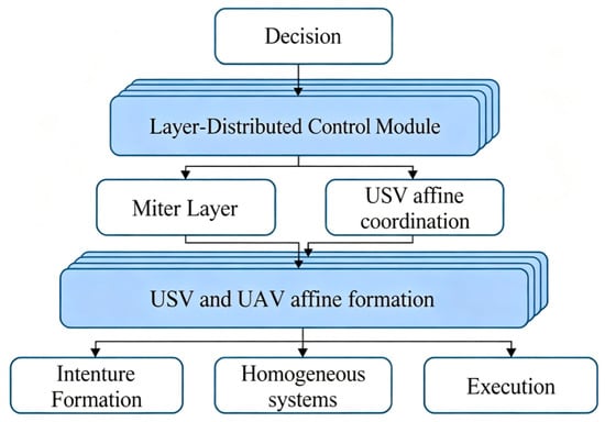
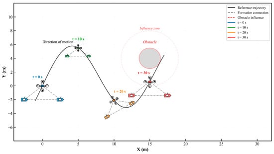
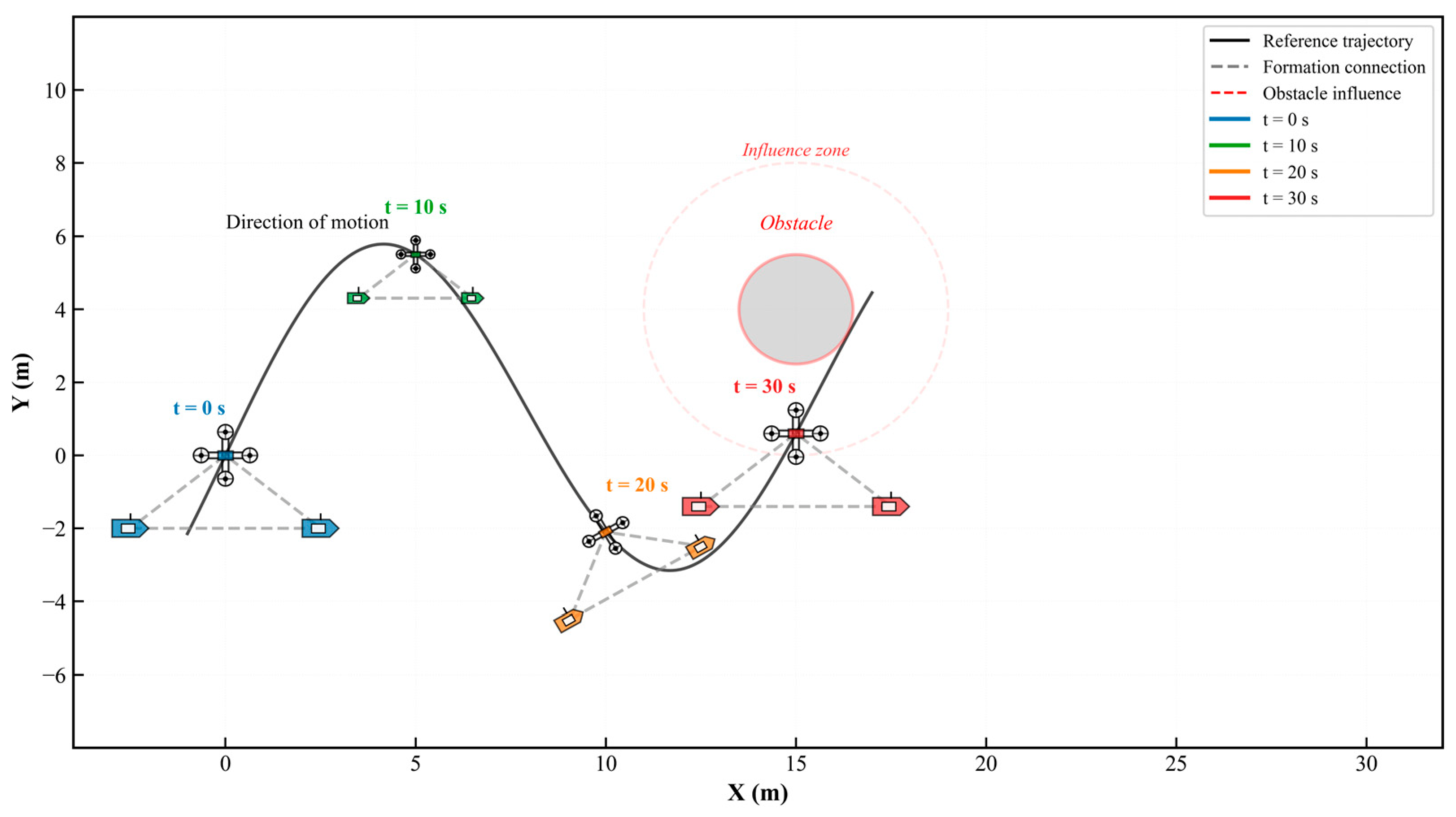
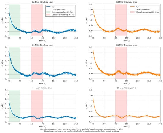
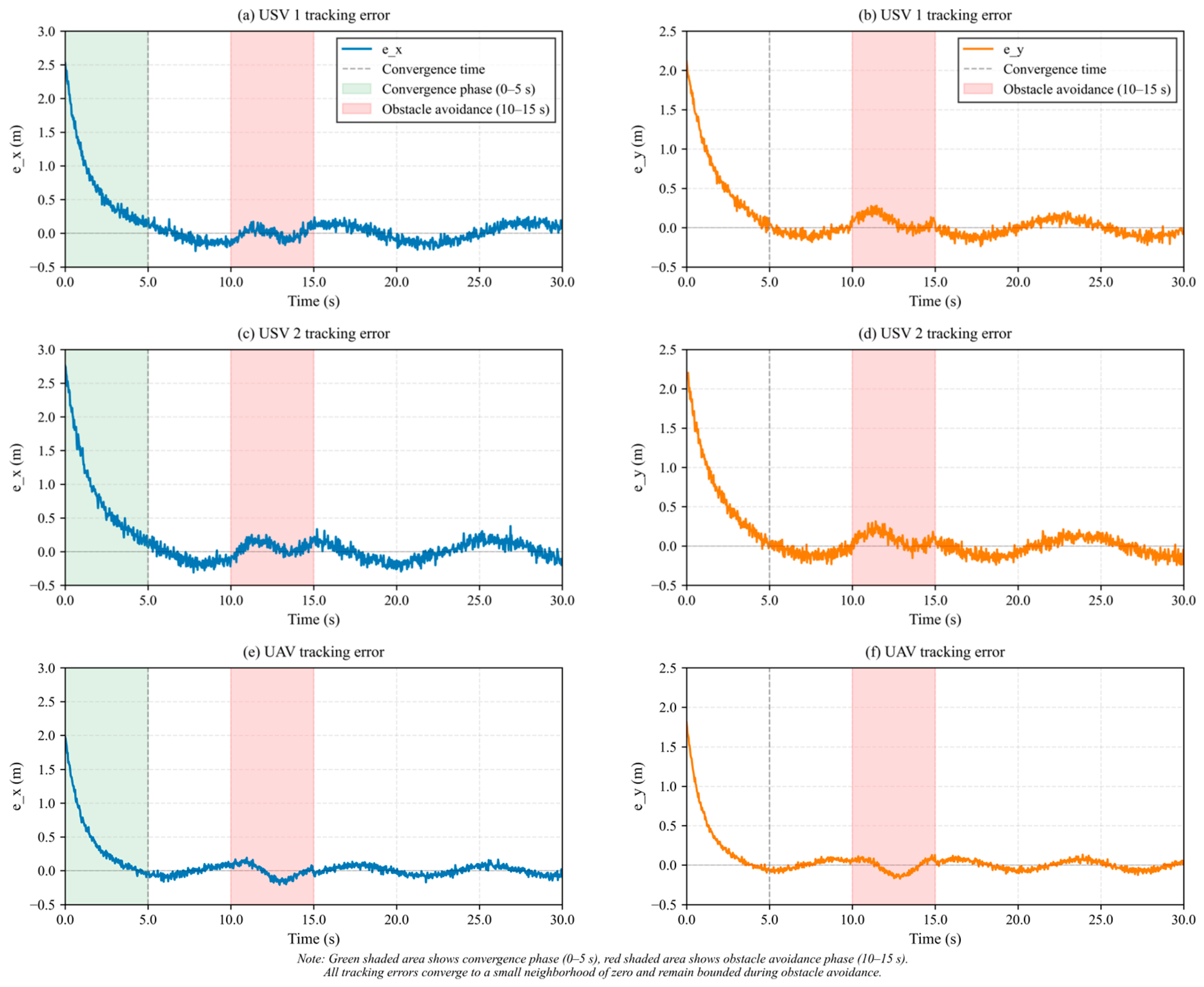
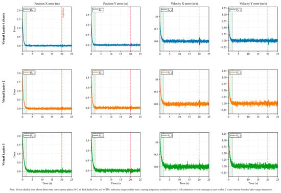
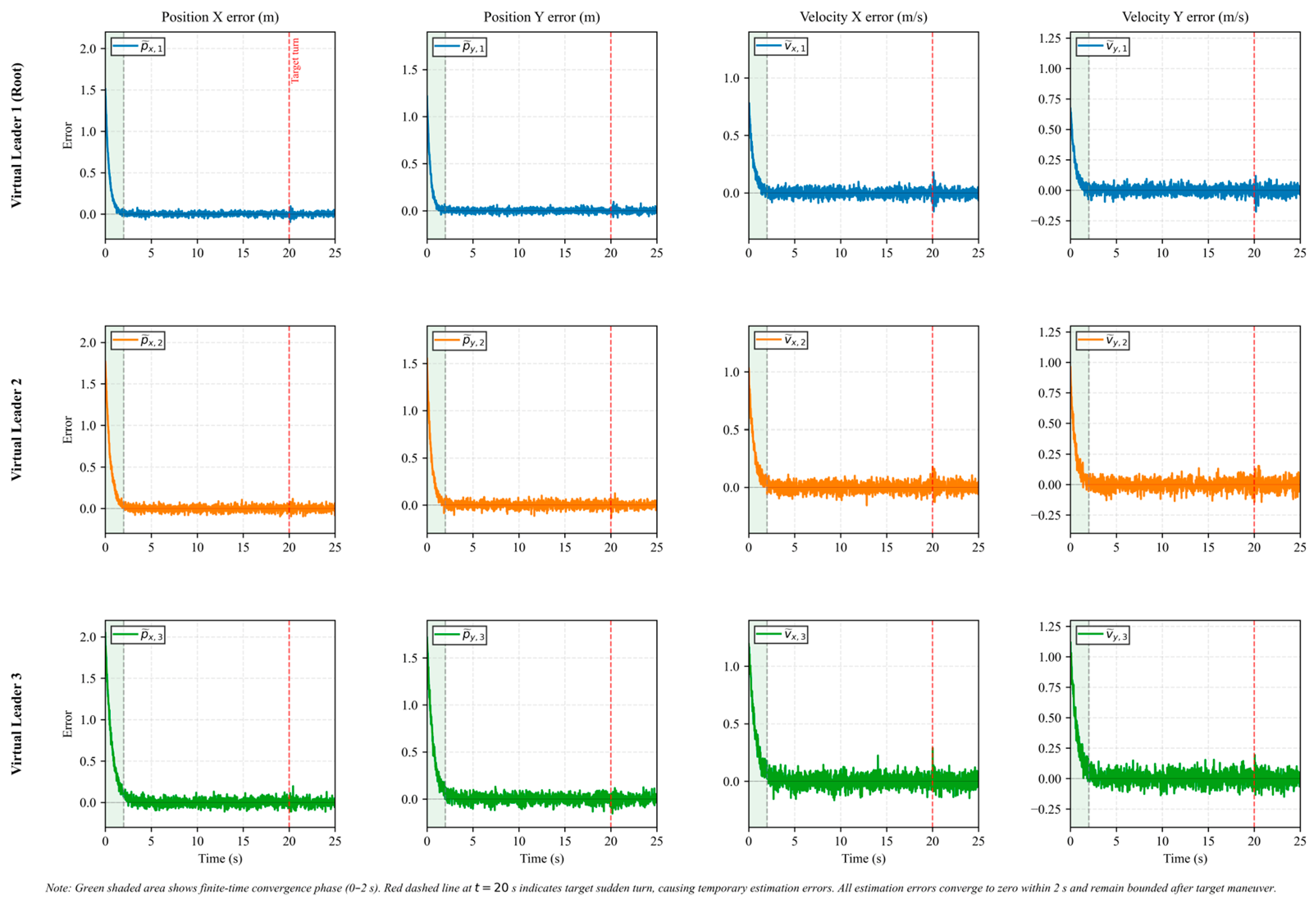
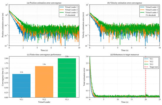
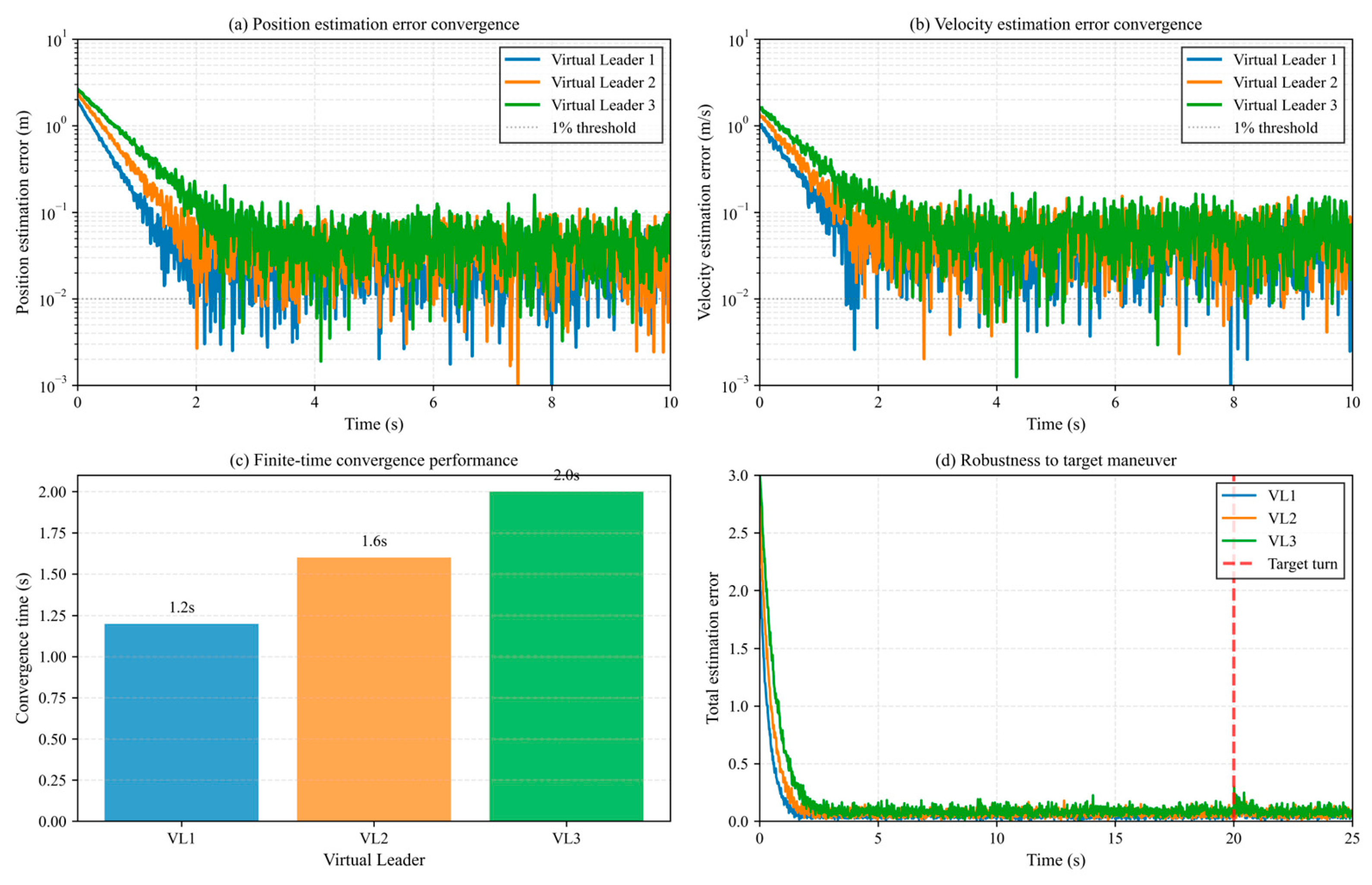
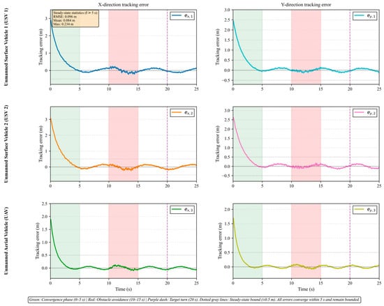
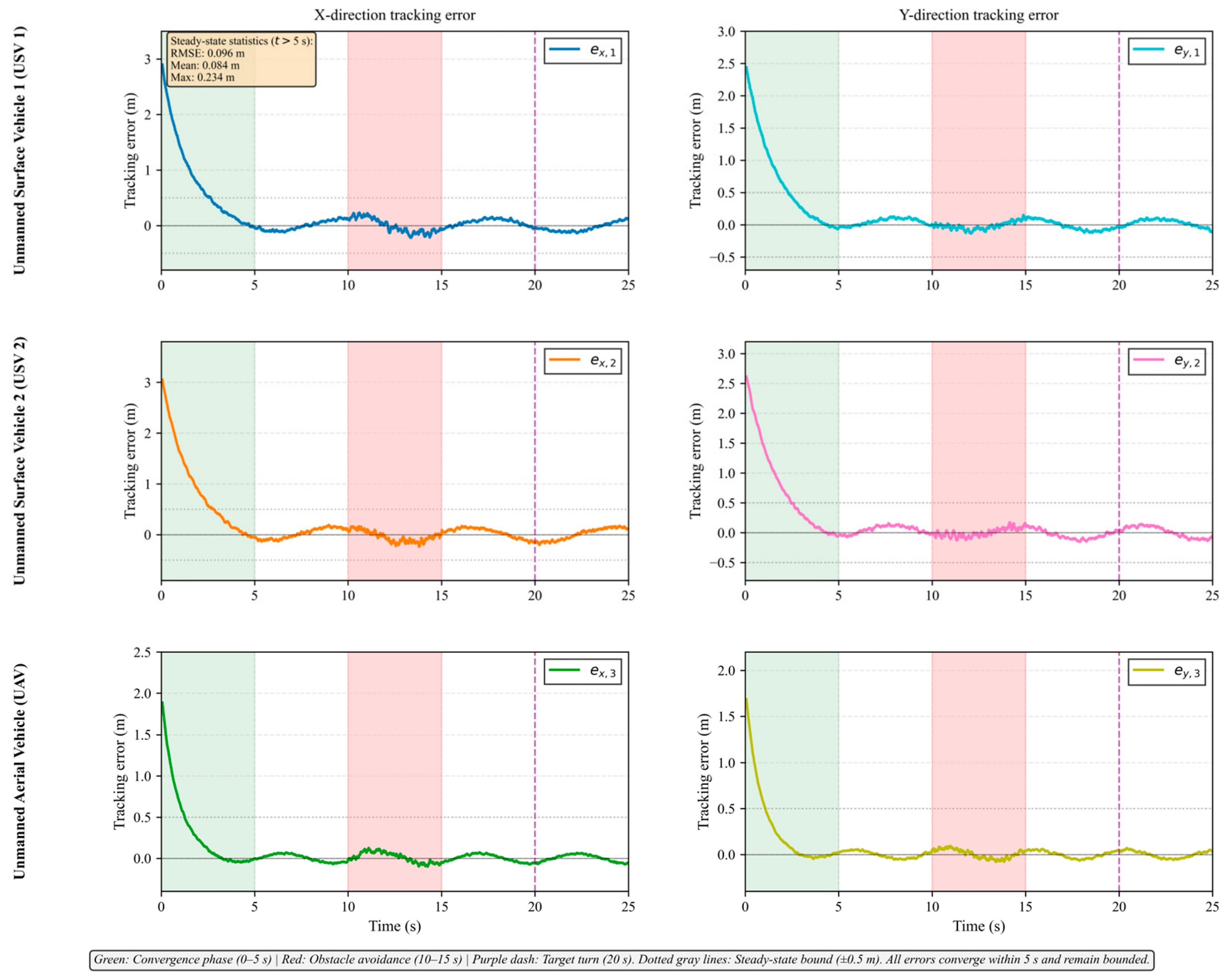
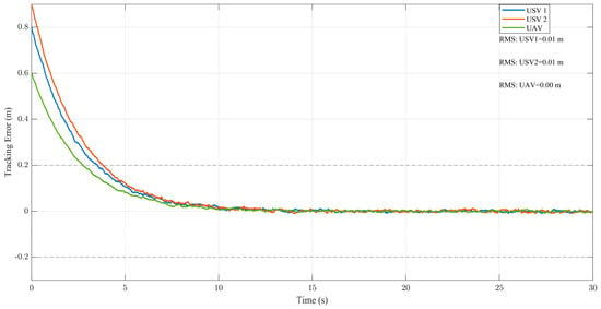
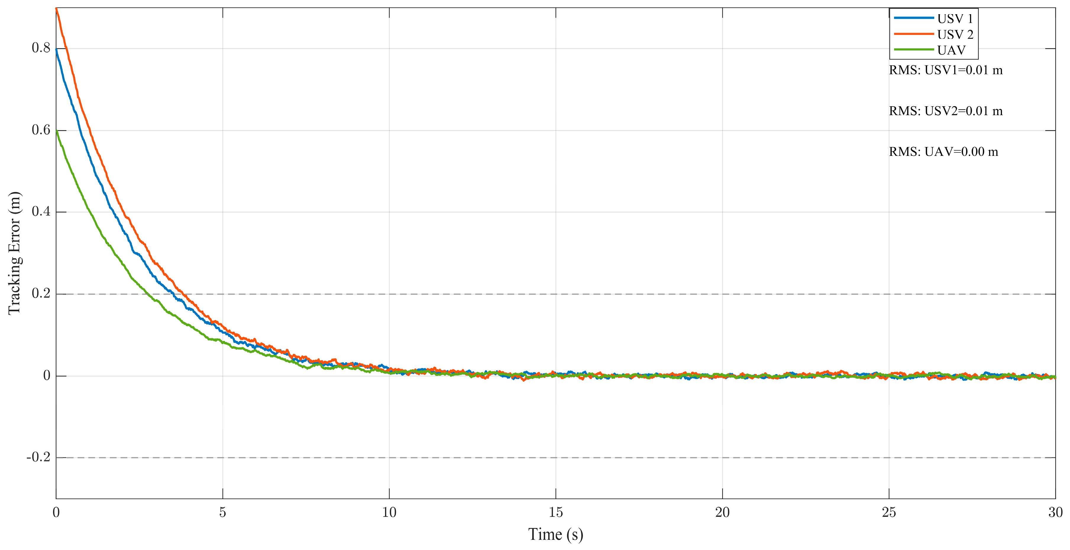
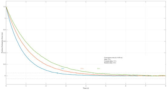
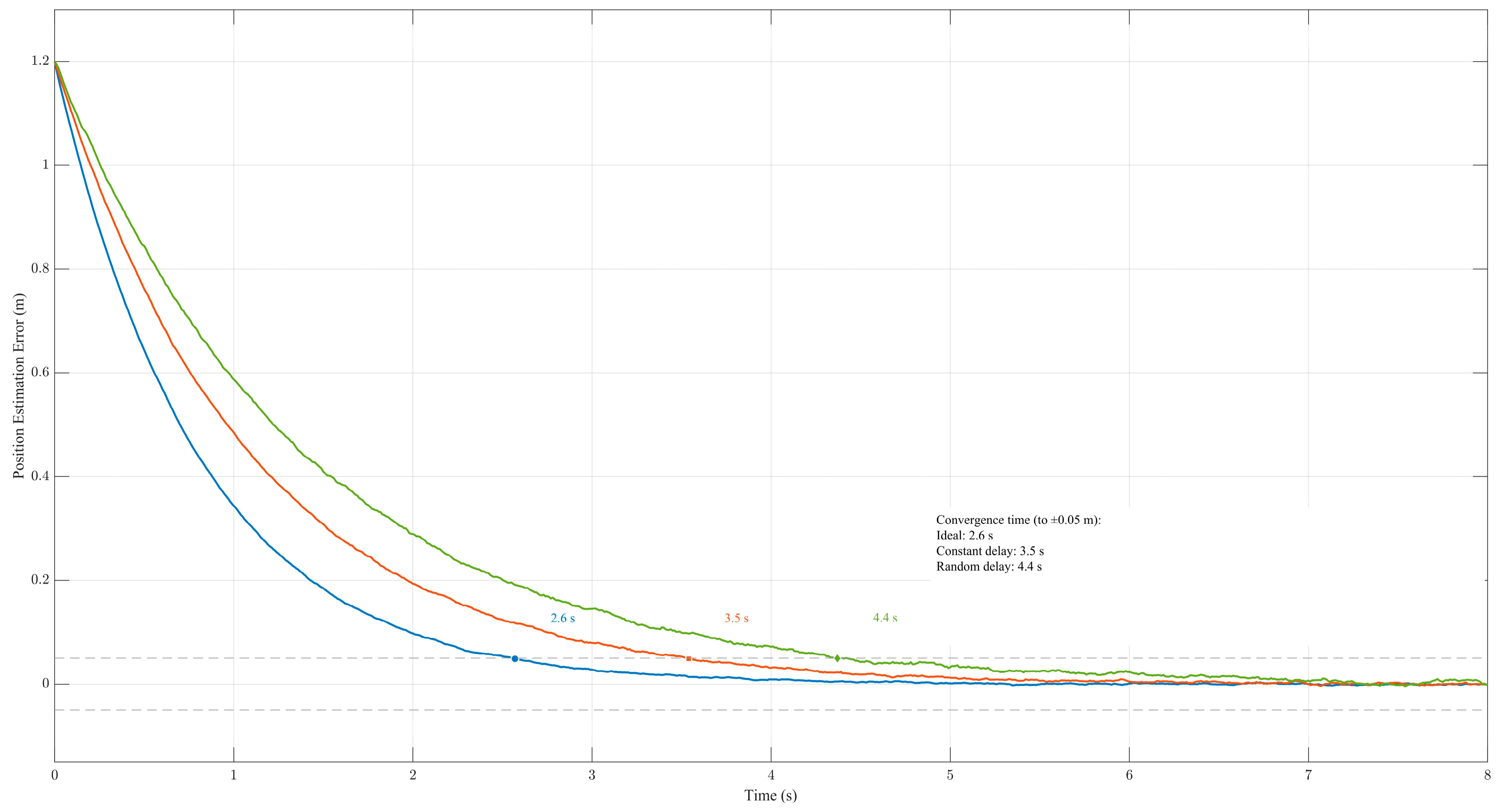
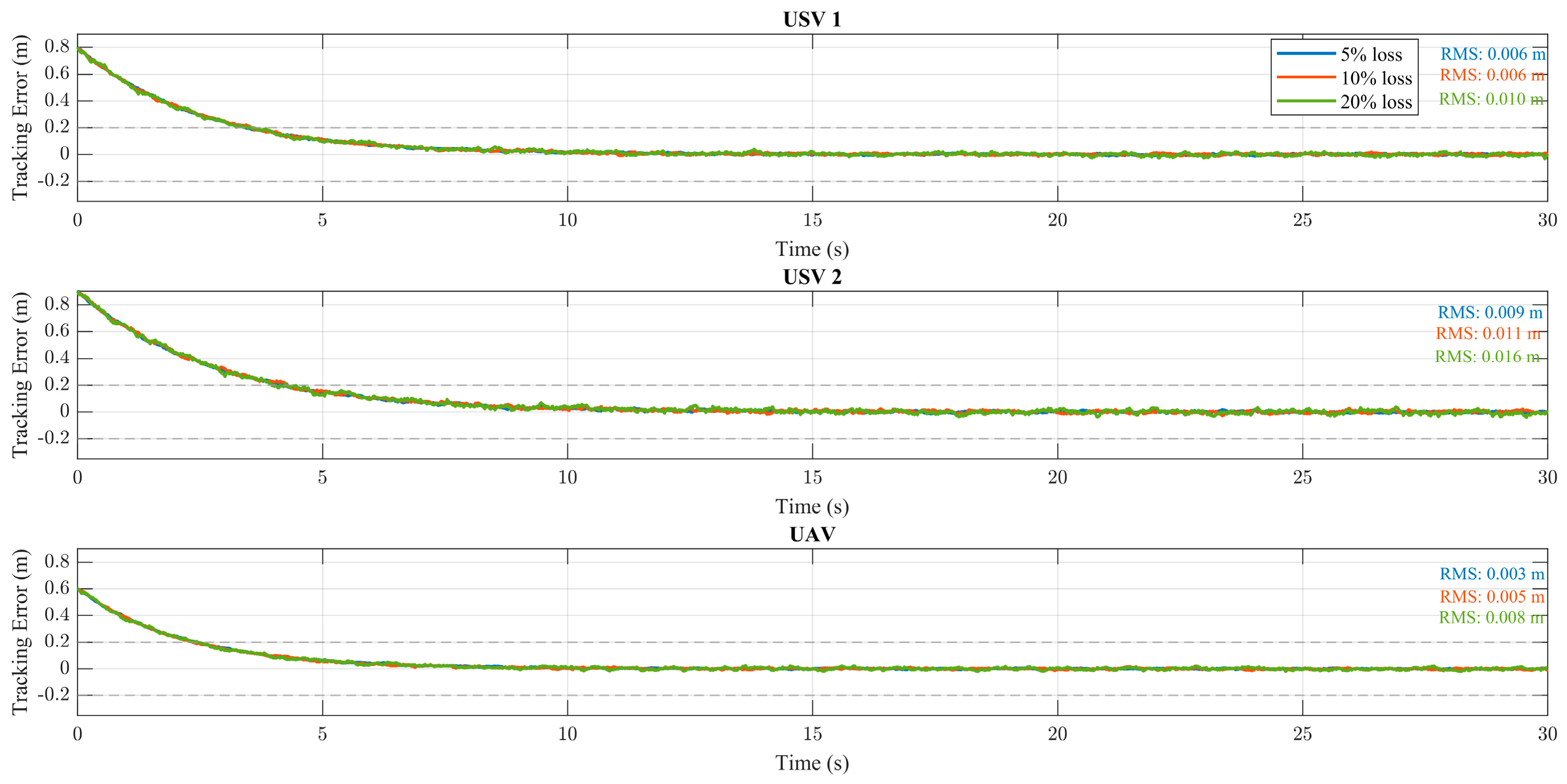
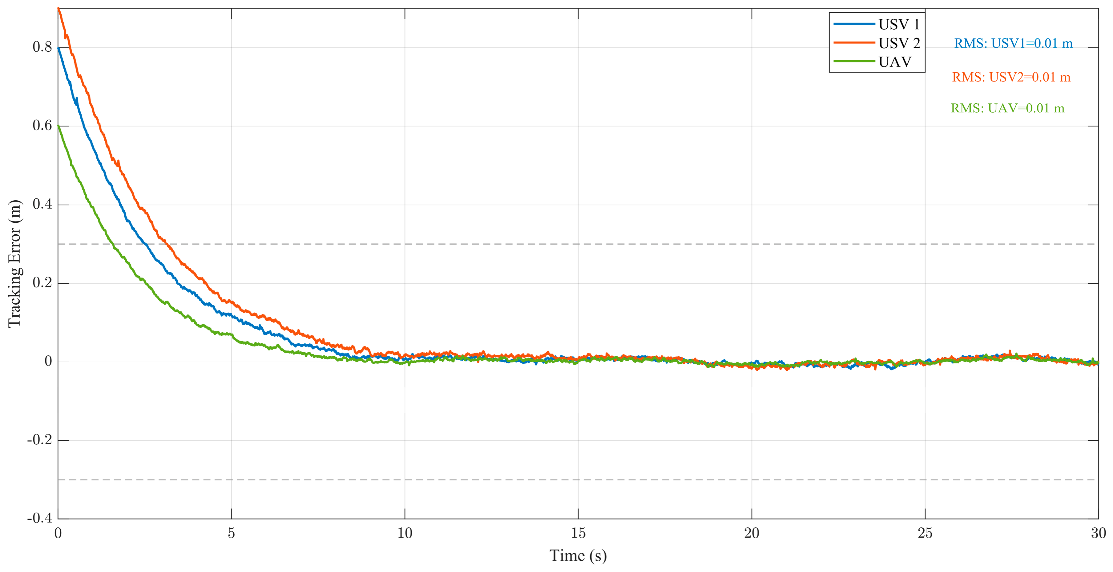
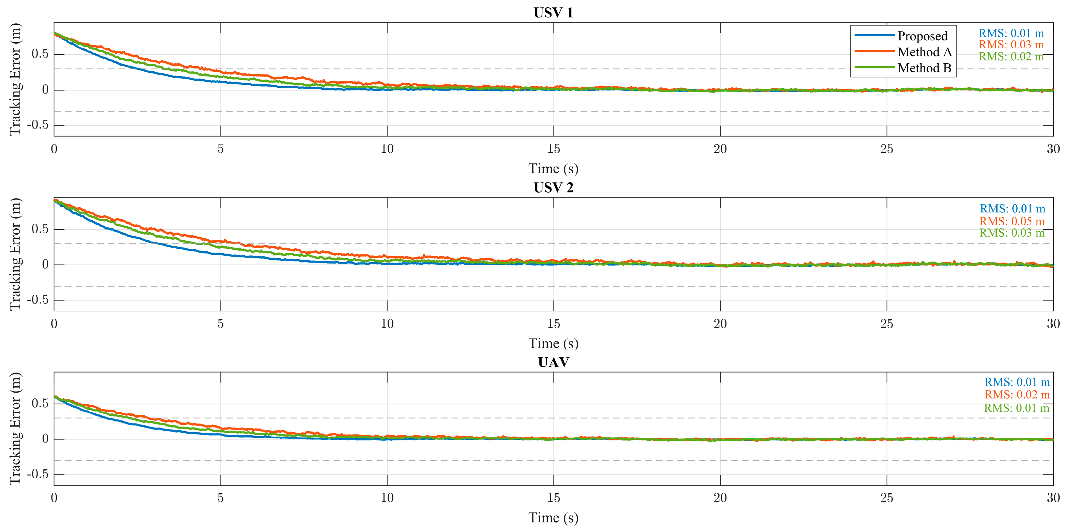
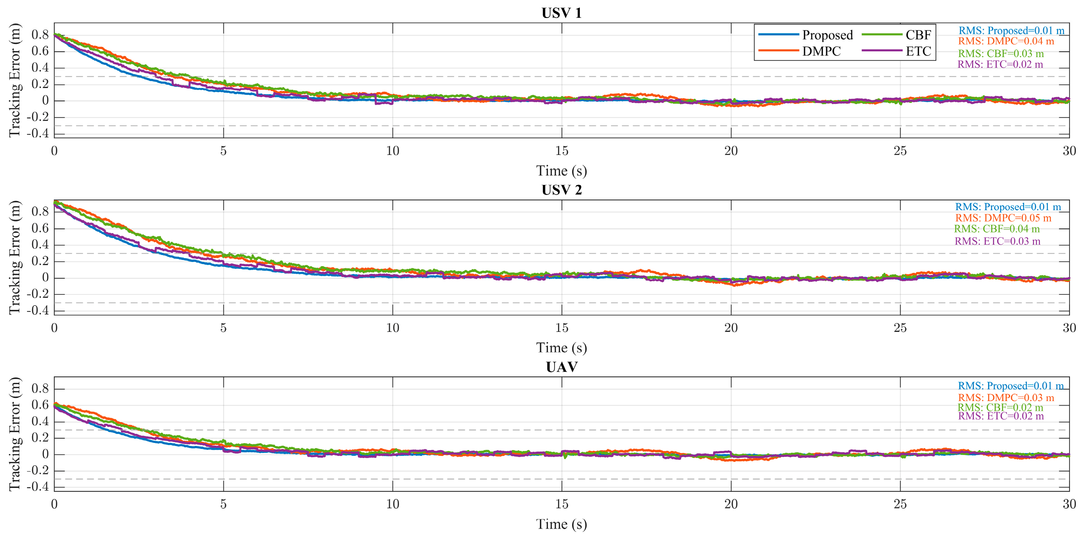

Disclaimer/Publisher’s Note: The statements, opinions and data contained in all publications are solely those of the individual author(s) and contributor(s) and not of MDPI and/or the editor(s). MDPI and/or the editor(s) disclaim responsibility for any injury to people or property resulting from any ideas, methods, instructions or products referred to in the content. |
© 2026 by the authors. Licensee MDPI, Basel, Switzerland. This article is an open access article distributed under the terms and conditions of the Creative Commons Attribution (CC BY) license.