


Abstract
Satellite radar altimetry provides the only global, all-weather record of significant wave height (SWH), but Sentinel-3 Level-2 retrievals retain systematic, context-dependent errors near coasts and at low sea states. We present a two-stage calibration that uses only Level-2 variables: a buoy-weighted isotonic regression removes the scale-dependent bias, and a LightGBM model predicts the residual from waveform-quality and along-track descriptors, with quantile models supplying a per-sample uncertainty. The method was evaluated on 10,234 Sentinel-3A/B overpasses collocated with 83 National Data Buoy Center (NDBC) buoys (2019–2024) under leave-one-buoy-out validation. The root-mean-square error with respect to the buoys fell from 0.266 m to 0.211 m (−21%; station-bootstrap 95% confidence interval of the reduction 0.038–0.073 m) and the bias from −0.113 m to +0.006 m. The gain was unchanged without buoy-dependent descriptors and persisted with nested hyper-parameter selection and in held-out years (2023–2024) but was uneven across regions. It was largest within 20 km of the coast and below 1.5 m. High sea states defined by the buoy value showed no RMSE reduction, a pattern consistent with regression dilution and buoy noise. After conformal rescaling, the 80% and 90% intervals reached nominal coverage on average at stations not used for fitting.
1. Introduction
Significant wave height (Hs), defined in modern practice as from the zeroth moment of the wave spectrum [1], is the primary descriptor of sea state for navigation, offshore and coastal engineering, wave-energy assessment and climate monitoring [2]. Satellite radar altimeters retrieve Hs from the slope of the leading edge of the radar echo and have produced a multi-decadal, globally calibrated record that underpins wave-climate studies [3,4,5,6]. The Copernicus Sentinel-3A/B constellation carries the SAR Radar Altimeter (SRAL), operated in delay-Doppler (SAR) mode, which narrows the along-track footprint to roughly 300 m and reduces measurement noise with respect to conventional pulse-limited altimetry [7].
The accuracy requirements that motivate this work are set by the way Hs enters engineering practice. Along most of the world’s coasts, including the Mediterranean, moored wave buoys are tens to hundreds of kilometres apart and their records rarely exceed two or three decades, so altimetry is often the only observation available where a structure is to be designed or a shoreline managed [2,8]. In these applications, errors in Hs do not propagate linearly. In the Hudson formula, the required armour-unit weight of rubble-mound breakwaters scales with the cube of the design wave height; in the formula of the Coastal Engineering Research Center (CERC), the longshore sediment transport rate scales with the 5/2 power of the breaking wave height; and wave overtopping depends exponentially on the ratio between crest freeboard and wave height [9]. A systematic error of 0.15 m on a 1.5 m sea state, the order of the raw Sentinel-3 bias at low sea states reported below, translates into errors of about 33% in the estimated armour weight and 27% in the longshore transport rate. Accumulated over a multi-year record, the same bias also shifts the return levels used for design and for coastal-risk assessment [8,10], which also depend on the long-term variability of mean sea level [11]. Nearshore accuracy matters most precisely where buoys are absent and altimetry is least reliable: in the 0–20 km coastal strip that controls erosion, dune retreat and harbour agitation.
Sentinel-3 SWH retrievals are nevertheless not uniformly accurate. Validation against buoys shows root-mean-square differences of roughly 0.3 m in the open ocean [12,13,14] but considerably larger errors within a few tens of kilometres of the coast, where land returns, bright targets and sharp sea-state gradients distort the waveform [15,16,17,18,19]. SAR-mode retrievals are also noisier at low sea states, where the leading edge becomes too steep to be resolved [14,20], and are sensitive to wave orbital velocity and to the direction of wave propagation relative to the ground track [21,22]. Part of the apparent coastal error is not instrumental at all: it stems from the representativeness mismatch between a point buoy measurement and a footprint-averaged retrieval and from the way altimeter and buoy records are paired in space and time [20,23,24,25,26].
Machine learning (ML) has been applied to sea-state problems along two main lines. The first replaces or augments the physical retracker with data-driven estimators that map waveform shape to Hs [27,28]. The second post-processes retrieved parameters, learning statistical corrections against in situ or model references [22,29,30,31]. For Sentinel-3, the two published calibrations closest to our work differ in scope. Atteia et al. [30] reduced SWH error from about 0.26 m to 0.10–0.12 m at two equatorial Atlantic sites but used a cross-calibrated altimeter product rather than buoys as the reference. Gou and Tourian [27] calibrated a simplified retracker in the North Sea and validated it against three buoys and model-based virtual stations, reducing near-coast errors from 1.51 m to 0.91 m. Neither study quantified per-sample predictive uncertainty or tested transfer to locations unseen during training, and both relied on a small number of in situ sites. More recent work on Sentinel-6 [22], HY-2B [26] and the wave spectrometer of the China–France Oceanography Satellite (CFOSAT) [32] shows that neural or tree-based corrections can bring SWH closer to NDBC buoys (e.g., 0.265 → 0.187 m) but either requires external reanalysis inputs or finds that scaling brings no benefit where buoys are well calibrated and far from the coast.
Two broader developments in remote-sensing data quality bear on how such corrections should be evaluated. First, the reference itself is uncertain. Triple-collocation studies report random errors of approximately 0.14–0.22 m for buoy Hs measurements, including potential contributions from representativeness differences associated with satellite–buoy collocations [33,34]. These errors are comparable in magnitude to those reported for satellite altimeters. Coastal assessments of the newest SAR-mode missions also show that agreement with in situ data depends strongly on distance to the coast and on the collocation criteria [20,35]. Second, there is growing emphasis on explaining the sources of model performance rather than reporting accuracy metrics alone: explainable artificial intelligence (AI) methods, chiefly SHapley Additive exPlanations (SHAP), are now the most common way of attributing model output to inputs in remote sensing [36], and conformal prediction offers a model-agnostic route to prediction intervals whose coverage is guaranteed when the data are exchangeable [37,38]. Both require care with spatially structured data, where random cross-validation overstates accuracy [39,40].
Three methodological questions therefore remain open and motivate this study. (i) How much can a correction built only from Level-2 variables, hence applicable at any point along the ground track without external inputs, reduce the error with respect to buoys? (ii) How much of that gain survives when the model is evaluated at buoys, regions and years it has never seen, i.e., under blocked rather than random validation [39,41,42]? (iii) Does the accompanying uncertainty estimate attain its nominal coverage at stations not used for fitting, so that it can be used to weight or reject corrected values?
We address these questions with a two-stage method (Figure 1). Stage 1 is a buoy-weighted isotonic regression [43] that removes the dominant scale-dependent bias under a monotonicity constraint. Stage 2 is a LightGBM gradient-boosted regressor [44,45] that predicts the residual from waveform-quality, geometric and seasonal features, complemented by quantile regressors [46] that yield a per-sample uncertainty width and feed a learned shrinkage factor. The two-stage isotonic + LightGBM calibration approach was originally developed and initially validated in a master’s thesis [47]. Building on this framework and its initial leave-one-buoy-out (LOBO) validation, the present study delivers the following additional contributions: (1) an independently reconstructed database of 10,234 Sentinel-3A/B–NDBC collocations at 83 stations over 2019–2024, and an extended evaluation of an ML calibration of Sentinel-3 SWH under LOBO, leave-one-region-out and time-blocked validation, with station-level confidence intervals and paired tests; (2) a set of ablations that separates the contribution of each component, including a linear baseline and a single-stage model; (3) an assessment of the coverage of the predicted uncertainty, with a conformal rescaling validated on stations not used for fitting; and (4) an analysis of conditions in which the method provides limited or no improvements, namely high sea states and open-ocean sites with already-low error, and of the possible causes, including regression dilution and the error of the buoy reference.
Figure 1.
Workflow of the two-stage calibration. xi: raw satellite SWH; zi: contextual Level-2 features computed along the track around the target point (Section 2.6); yi: buoy SWH, used only to train and validate both stages (dashed arrows) and never required at inference. Stage 1 removes the global, scale-dependent bias; Stage 2 predicts the residual and the interval width ui; the optional learned shrinkage is detailed in Section 2.7. Symbols are defined in Section 2.4, Section 2.5, Section 2.6 and Section 2.7. The asterisk in g* denotes the fitted Stage 1 mapping of Equation (2).
2. Materials and Methods
2.1. In Situ Reference: NDBC Buoys
Hourly or half-hourly Hs records (variable WVHT of the standard meteorological files) were obtained from the historical archive of the National Data Buoy Center (NDBC; https://www.ndbc.noaa.gov/ (accessed on 14 October 2026)) for the 83 moored stations used in the original study (Figure 2), covering January 2019 to December 2024. NDBC derives Hs from the heave spectrum measured by hull-mounted accelerometers, with automated quality control [48]. Inter-comparison studies indicate an Hs accuracy of roughly 0.1–0.2 m with small long-term drift [49,50], although buoy response can degrade in extreme seas [51]. Triple-collocation analyses place the random error of buoy Hs, including the representativeness error of the pairing, between about 0.14 m [33] and 0.22 ± 0.02 m [34]. Records flagged as missing (WVHT = 99) were discarded; the remaining values were used unaltered as the reference. NDBC does not distribute a history of mooring positions, and moored buoys are periodically redeployed. Station coordinates were taken from the NDBC station pages and checked against the positions stored, for every station, in the collocation database of the original study. For station 42058 (central Caribbean), the currently listed position lies about 96 km from the 2019–2024 mooring, and the latter (14.512° N, 75.153° W) was used; with it, all 88 overpasses of the station coincide with those of the original database. For the remaining 82 stations, the two sources agree within 1 km at 72, differ by 1.3–4.1 km at 7 and by 9.6–12.7 km at 3 (41001, 41040 and 42060). These offsets are small compared with the 20 km search radius but are not negligible, so a sensitivity test excluding the affected stations is reported in Section 3.6.
Figure 2.
Locations of the 83 NDBC stations used in this study, coloured by the regions of Table 1 (Section 2.1).
For stratified analyses, the stations were grouped into three regions. The North Pacific group comprises the stations of the north-eastern Pacific and the Bering Sea, whose World Meteorological Organization (WMO) identifiers begin with 46 (29 buoys). The Tropical group comprises the stations of the central and western tropical Pacific, with identifiers beginning with 51 and 52, together with all other stations south of 25° N, including the southern Gulf of Mexico, the Caribbean and the tropical western Atlantic (28 buoys). The North Atlantic group comprises the remaining Atlantic and northern Gulf of Mexico stations (26 buoys). Latitudes range from 14.3° S to 59.9° N. Table 1 summarises the composition of the database.
Table 1.
Composition of the quality-controlled collocation database (2019–2024). P10–P90: 10th–90th percentiles of buoy Hs.
2.2. Sentinel-3 SRAL Level-2 Data
Sentinel-3A and -3B SRAL Level-2 marine products (SR_2_WAT, non-time-critical timeliness, processing baseline 005) were identified through the catalogue of the Copernicus Data Space Ecosystem (https://dataspace.copernicus.eu/ (accessed on 14 October 2026)) by intersecting each product footprint with a box of ±21 km around each buoy (20 km search radius plus a 1 km buffer). For 2019 to early 2023, the products belong to the 2023 reprocessing campaign; afterwards, they are the operational products of the same baseline (7045 and 3189 of the final events, respectively). Only the required variables were read from each enhanced_measurement.nc file, through partial HTTP range requests on the Copernicus S3 object store, which avoids the download of the full ≈ 50 MB product. The 20 Hz Ku-band variables extracted were [52]: SWH (swh_ocean_20_ku), surface type and the SWH and σ0 quality flags, backscatter coefficient σ0 (sig0_ocean_20_ku), automatic gain control (AGC, agc_20_ku), mean quadratic error of the waveform fit (MQE, mqe_ocean_20_ku), peakiness (peakiness_2_20_ku), thermal noise, number of retracker iterations, distance and angle to the nearest coast, retracked and tracker range (range_ocean_20_ku, tracker_range_20_ku), and the ionospheric correction.
2.3. Quality Control and Collocation
Only 20 Hz records with surf_type_20_ku = 0 (open ocean), zero SWH and σ0 quality flags, and 0 ≤ Hs < 30 m were retained. For each product (i.e., each satellite overpass), the valid records within a great-circle distance d ≤ 20 km of the buoy were selected; the overpass time ts was taken as the median time of these records and paired with the buoy record closest in time, provided |ts − tb| ≤ 30 min. Each overpass therefore yields at most one collocation event per buoy. The 20 km radius is stricter than the 25–50 km windows commonly used in open-ocean validation [12,26], a choice motivated by the rapid spatial decorrelation of sea state near the coast [20]. Within each event, the satellite records were aggregated to their median, mean, standard deviation and inter-quartile range (IQR), for SWH and every auxiliary variable; the median SWH was used as the satellite estimate xi. Where the same overpass was available both as a reprocessed and as an operational product, the reprocessed one was kept. The buoy enters this construction only as the centre of the 20 km window: the same along-track statistics can be computed around any target point crossed by the ground track, with or without a buoy. Three descriptors, in contrast, exist only because a buoy is present: the minimum and median distance of the records from the buoy and the time separation of the pair. Records flagged as invalid by the Level-2 processor were excluded, so the results apply to flag-valid retrievals; the hardest coastal cases, in which the processor rejects most records, are not addressed.
Two event-level quality criteria were defined before model fitting: at least 10 valid 20 Hz records (≈0.5 s, i.e., ≈3.4 km of track) and a within-event SWH IQR not larger than 2 m. They remove events derived from only a few contaminated records, in which the median SWH can be meaningless (up to 19.8 m against a buoy value of 2.4 m in our data). Of 10,356 candidate events, 122 (1.2%) were removed and 10,234 retained, with all 83 stations represented (27 to 275 events per station). For transparency, the main results without this filter are also reported (Section 3.1). The median number of 20 Hz records per event is 84 (5th percentile 27). The median distance of the closest record to the buoy is 11.0 km, and the median time separation is 10.5 min. The sampling is skewed towards the coast (Figure 3a): 40.9% of the events lie within 20 km of the nearest coastline, 35.2% between 20 and 200 km and 23.9% beyond 200 km. Sentinel-3A contributes 4755 events and Sentinel-3B 5479.
Figure 3.
(a) Number of collocation events per logarithmic distance-to-coast bin; (b) predicted interval width ui (median and inter-quartile range under LOBO) versus distance to coast.
The pairing differs from that of the original thesis, in which every buoy record within ±30 min of an overpass formed a separate event; with half-hourly or 10-min buoy records, this repeats the same satellite value up to several times per overpass and inflates the sample size (19,019 events in the thesis) without adding independent information, mostly at the high-rate coastal stations. One event per overpass is the more conservative choice for the statistical analyses of Section 2.9.
2.4. Error Model and Notation
For collocation event i let hi denote the true significant wave height over the altimeter footprint, yi the buoy value and xi the (median) raw satellite value. We write
where εb collects buoy measurement error and representativeness error, β(⋅) is the (unknown, possibly non-linear) systematic response of the Level-2 retrieval and εs its random retrieval error; εb and εs are assumed to be independent of each other [23,24]. The goal is an estimator of hi built from xi and from a vector zi of contextual Level-2 variables, trained against yi. Because yi is itself a noisy proxy of hi, every buoy-trained calibration estimates E[y∣x,z] rather than h; the consequences are made explicit in Section 2.5.
2.5. Stage 1: Buoy-Weighted Isotonic Calibration
Stage 1 estimates the non-decreasing function g* that minimises the weighted squared error
solved exactly by the pool-adjacent-violators algorithm [43]; the solution is piecewise constant on the training knots, is linearly interpolated between knots and is held constant outside the training range, so that the calibrated SWH of event i, Hcal,i = g*(xi), is a continuous and non-decreasing function of xi. The weights
assign every buoy the same total weight irrespective of its number of events NB(i). Monotonicity is a shape constraint that prevents rank inversions and limits the effective degrees of freedom; it is not a physical law, and we treat it as a regularisation.
Equation (2) is a regression of y on x and therefore estimates E[y∣x]. Under the error model (1), with β locally linear and εs of variance , the slope of E[y∣x] with respect to the noise-free signal is attenuated by the reliability ratio
so that a calibration unbiased conditional on x is necessarily biased conditional on y: to first order,
where μy is the mean of the training distribution. Equation (5) predicts a bias that is negative below μy, positive above it and grows linearly with y with slope (1 − λ), the regression-dilution (errors-in-variables) effect. Equation (5) neglects the buoy error εb. Under the additive, locally linear error model (1), with εb independent of h, including it adds a tilt of the same sign, so the slope observed against the buoy value is an upper bound on 1 − λ (Section 3.4). The equation still provides an empirical check: after calibration, the bias should be close to zero when stratified by the estimate and should grow with the buoy value when stratified by it. The same mechanism explains why long-term altimeter calibrations use reduced-major-axis rather than ordinary regression [3]. The conditional bias is reported both ways (Section 3.4).
2.6. Stage 2: Residual Prediction with Gradient Boosting
The Stage 1 residual ri = yi − Hcal,i is modelled as , where f is an additive ensemble of M regression trees Tm fitted by gradient boosting with learning rate ν [44,45],
with the L1 (absolute-error) objective, so that estimates the conditional median of the residual and is robust to occasional very large buoy–satellite discrepancies, and Ω the usual leaf-count and L2 penalties. The feature vector z (36 features) deliberately excludes the satellite SWH itself (raw or calibrated), so that Stage 2 cannot re-learn the global calibration. It comprises five groups: (i) Waveform-quality and instrumental descriptors: the within-event mean and coefficient of variation (CV) of σ0, AGC, MQE, peakiness, thermal noise, retracker iterations, retracked range, tracker range and ionospheric correction. (ii) Along-track geometry: mean and CV of distance and angle to coast, log(1 + dcoast), number of valid 20 Hz records and a Sentinel-3B indicator. (iii) Pairing descriptors: minimum and median distance of the records to the buoy and time separation of the pair. (iv) Position: sine and cosine of the latitude and longitude of the buoy. (v) Seasonality: sine and cosine of month and day of year. Groups (i), (ii) and (v), and the coordinates of group (iv), can be computed for any target point along the ground track; group (iii) exists only where a buoy is present, and Section 3.6 shows that removing it together with group (iv) leaves the performance unchanged. The coefficient of variation is CV = std/(|mean| + δ) with δ = 10−6 in the units of each variable (the symbol δ is used to avoid confusion with the error terms of Equation (1)). Only two variables change sign and can have a mean close to zero: the angle to coast (smallest absolute event mean 0.002°) and the ionospheric correction (39 events with an absolute mean below 10−3 m). For these events, the CV becomes large but remains finite; because tree splits depend only on the ordering of the values, such values fall in the extreme bins of the feature and do not destabilise the fit. Remaining gaps (≤0.4% per feature) are handled natively by LightGBM. Compared with the original thesis implementation, which included all numeric along-track statistics available, several inputs were deliberately excluded. The within-event standard deviation and inter-quartile range of the satellite SWH, the 1 Hz altimeter wind speed, and the sea-state-bias correction were omitted because they are functions of the retrieved sea state and would reintroduce the quantity being corrected into Stage 2; their potential contribution to predictive performance was not evaluated in this study. The rain fraction was also excluded, and its predictive contribution was not assessed either. The wet tropospheric correction is absent from the 2019–2022 products used in the thesis. The medians and inter-quartile ranges of the auxiliary variables were omitted as largely redundant with their means and coefficients of variation. We note that σ0 and peakiness are themselves functions of sea state, so the separation between the two stages is hierarchical rather than orthogonal, and that adding does not formally preserve the monotonicity of Stage 1; the rate of rank inversions is reported as a diagnostic.
Hyper-parameters were selected by random search over 24 configurations (number of leaves {7, 15, 31, 63}, learning rate {0.01, 0.03, 0.05, 0.1}, number of trees {200, 400, 800}, minimum samples per leaf {20, 40, 80, 150}, feature fraction {0.6, 0.8, 1.0}, L2 penalty {0, 1, 5, 20}; bagging fraction 0.8), each scored by the buoy-weighted mean absolute error (MAE) of the Stage 1 residual under 5-fold cross-validation grouped by station. The folds were assigned deterministically (station identifiers sorted and allocated to the five folds in rotation) and LightGBM was run in deterministic mode with a fixed seed, so that the selection and all subsequent results are exactly reproducible with the code and library versions provided (Data Availability Statement). The selected configuration (7 leaves, learning rate 0.05, 200 trees, at least 40 samples per leaf, feature fraction 1.0, no L2 penalty; cross-validated MAE 0.142 m; range 0.142–0.147 m over the 24 configurations) was used for all models except those of experiments N2 and N3, which repeat the selection in a nested design (Section 2.8).
2.7. Uncertainty Estimation and Learned Shrinkage
Two further boosted ensembles , τ ∈ {0.1,0.9}, with the same hyper-parameters as the median model, are fitted with the pinball (quantile) loss [46]
so that and estimate the 10th and 90th conditional percentiles of the residual. Because the two quantile models are fitted independently, their predictions may cross; crossings are removed by ordering the two values for each event. The per-sample predictive uncertainty is the width of the resulting nominal 80% interval,
The 80% level was chosen because the 10th and 90th conditional percentiles are estimated from many more events in the tails than the 5th and 95th, which matters for the narrow strata (coastal, high sea states) analysed in Section 3. Engineering applications often require wider intervals, so a nominal 90% interval (τ ∈ {0.05,0.95}) was also fitted and validated in the same way (Section 3.5).
The final estimate applies a per-sample shrinkage to the predicted residual (Figure 4),
Figure 4.
Uncertainty-aware learned shrinkage (Stage 2 kML). The quantile models give the interval width ui (Equation (8)); the auxiliary model gkML, trained on out-of-fold predictions to reproduce the target of Equation (10), returns the factor applied in Equation (9). The asterisk denotes the oracle shrinkage factor of Equation (10), which the auxiliary model is trained to reproduce.
For a known residual ri, the factor that minimises over k ∈ [0,1] is the oracle shrinkage
which equals 1 when the prediction is correct in sign and not too large, and 0 when it has the wrong sign. The ratio is undefined for and unstable near zero, so in the code, the denominator is replaced by ±10−3 m, with the sign of , whenever m. The auxiliary model gkML (200 trees, 15 leaves, squared-error loss) predicts from zi, , , ui and , and its output is clipped to [0,1]; its training targets are built from out-of-fold predictions of an inner 5-fold cross-validation grouped by station. The variant with is referred to as Stage 2 full, whereas the variant with the learned factor is called Stage 2 kML. Because the learned shrinkage did not improve the results (Section 3.1), it is retained only as a documented negative result.
2.8. Validation Protocol
All main results are reported under LOBO cross-validation, a spatially blocked design [41] that mimics deployment at a site without in situ data: for each of the 83 stations, Stage 1, Stage 2, the quantile models and the shrinkage model (including its inner cross-validation) are re-fitted on the remaining 82 stations and applied to the held-out one, and the 83 held-out prediction sets are pooled. Because neighbouring stations experience correlated conditions, LOBO is complemented by two more stringent designs: leave-one-region-out (each of the three regions of Table 1 held out in turn) and a time-blocked split (training on 2019–2022, testing on 2023–2024 at all stations). In the main runs the hyper-parameters were selected once, by the grouped cross-validation of Section 2.6 on all stations, and then held fixed, so the held-out station contributed to the choice among the 24 configurations. Because such selection can bias error estimates optimistically [53], the selection was repeated in a fully nested design (experiment N2): the stations were divided deterministically into 10 outer groups (sorted identifiers allocated in rotation), and for each outer group, the complete 24-configuration search, with its own 5-fold grouped inner cross-validation, was run on the stations of the other nine groups only. The outer predictions of this nested run were compared with those of a run on the same 10 outer groups in which the hyper-parameters were held at the original, non-nested selection. Ten outer groups rather than 83 were used to keep the cost within reach (10 inner searches of 24 configurations per model, i.e., 240 configuration evaluations and 1200 inner fits); each outer group still withheld about eight stations, so this design was more stringent than LOBO. The nested selection was also run with the feature set of N1a (experiment N1a + N2), which is the configuration recommended for operational use.
To isolate the contribution of each component, the following ablations were run under the same LOBO protocol: (A) ordinary least-squares (OLS) linear calibration in place of Stage 1, alone and followed by Stage 2; (B) unweighted isotonic regression; (C) a single LightGBM model that includes the raw SWH among its features (one stage, no isotonic step); (D) Stage 2 without latitude/longitude encodings; (E) Stage 2 without seasonal encodings; (N1a) Stage 2 without the pairing descriptors and the coordinate encodings (groups (iii) and (iv) of Section 2.6); (N1b) the same configuration, additionally excluding the number of valid 20 Hz records. Sensitivity to the collocation window (H) was assessed by restricting the evaluation, and separately the training, to events with closest distance ≤ 10 km and/or time separation ≤ 15 min, and sensitivity to station positions (N10) by excluding the stations whose position differs from that of the original database by more than 1 km or 5 km (Section 2.1). In A and C, the residual-model hyper-parameters of the reference were reused; because this can favour the reference, both baselines were also re-run in the nested design with their own 24-configuration search (experiment N3: the single-stage model is tuned on the buoy SWH, the OLS variant on its own residual). Except for the single-stage models (C and the single-stage run of N3), all experiments used Stage 2 full. Finally, the sea-state threshold discussed in Section 4.5 was applied to the Stage 1 estimate, which is available without a buoy (N5): Stage 2 full below the threshold, Stage 1 above it.
2.9. Metrics and Statistical Assessment
For a set of n held-out events with residuals we report the bias (positive when the estimate is lower than the buoy), the root-mean-square error , the mean absolute error (MAE), the scatter index and the Pearson correlation R. Because events are clustered by station and serially correlated within a station, uncertainties are obtained by a cluster bootstrap: stations are resampled with replacement (B = 2000 replicates), each metric (or difference of metrics between two methods evaluated on the same resample) is recomputed on the pooled resampled events, and 95% percentile confidence intervals (CI) are reported for the RMSE, bias, MAE and correlation (bootstrap seed 0). Differences between methods are also tested with the paired Wilcoxon signed-rank test [54] on the 83 per-station RMSE values, which treats the station as the unit of replication. The calibration of the predictive intervals is assessed by the empirical coverage
whose nominal value is 0.80. Where C falls short, a split-conformal rescaling in the spirit of conformalised quantile regression [37,55] is applied: the factor c is the empirical quantile, at the nominal level, of the scores on a set of calibration stations, and the rescaled interval is . Its coverage is assessed in two designs. (a) LOBO scores: the stations are split at random into a calibration half and a test half (seed 1), and the split is repeated 500 times to measure the sensitivity of c and of the test coverage to the partition. Each LOBO score is a leave-one-station-out residual, but the model that predicts a test station was trained on the calibration stations, so this design is close to, but not exactly, a split-conformal setting [38]. (b) Three-way split with nested selection: the stations are divided at random into a training set (50%, 41 stations), a calibration set (25%, 20 stations) and a test set (25%, 22 stations) (seed 11). The Stage 2 hyper-parameters are selected on the training stations only, with the 24-configuration search and 5-fold grouped inner cross-validation of experiment N2, and Stage 1, Stage 2 and the quantile models are then fitted on the same stations, so that neither the calibration nor the test stations contribute to model selection or fitting. Design (b) uses the feature set without pairing descriptors and coordinates (N1a), which is the configuration recommended for operational use (Section 4.6). The factor c is the quantile of the calibration scores at the level α(1 + 1/n), where α is the nominal coverage and n the number of calibration events, and the coverage is evaluated on the test stations. Design (b) is repeated 20 times for the 80% and 90% intervals. The station allocation of every repetition is reproduced by the code from the stated seeds. In operation, the factor would be estimated in the same way, on calibration stations not used to fit the final model; the spread of c over the repetitions of designs (a) and (b), reported in Section 3.5, measures its sampling variability and is not a set of values to choose from. The intervals quantify the buoy-referenced discrepancy, which includes buoy measurement and representativeness errors; they should therefore not be interpreted as direct estimates of retrieval-only uncertainty.
Feature contributions to Stage 2 are summarised by the mean absolute SHAP value [36,56], computed for each of the 83 LOBO models on the events of its held-out station and pooled. The stability of the ranking is measured by the range of ranks of each feature across the 83 models. Because a held-out station contributes on average about 120 events, too few for a stable ranking; these ranks are computed from 1500 training events sampled from each LOBO model (seed equal to the fold index). All computations used Python 3.13 with scikit-learn 1.9.1, LightGBM 4.7.0, SHAP 0.53.0, NumPy 2.5.3, pandas 3.0.5, SciPy 1.18.1 and Matplotlib 3.11.2.
3. Results
3.1. Global Performance
Table 2 pools the 10,234 LOBO predictions, and Figure 5 shows the corresponding scatter plots. The raw Level-2 SWH has an RMSE of 0.266 m and a bias of −0.113 m, i.e., the altimeter reads higher than the buoys on average. Stage 1 removes the bias (+0.003 m) and lowers the RMSE to 0.241 m (95% CI of the reduction −0.036 to −0.015 m; Wilcoxon p = 0.0004; 51 of 83 stations improved). Stage 2 full reaches 0.211 m, a reduction of 0.055 m with respect to the raw product (−21%; station-bootstrap 95% CI −0.073 to −0.038 m; Wilcoxon p < 10−4; 68 of 83 stations improved) and of 0.029 m with respect to Stage 1 (95% CI −0.039 to −0.021 m; p < 10−4; 71 of 83 stations improved). The scatter index falls from 0.161 to 0.128, and the correlation rises from 0.973 to 0.979. The learned shrinkage does not improve on Stage 2 full: Stage 2 kML is 0.004 m worse (95% CI +0.000 to +0.007 m; p = 0.003; better at only 27 of 83 stations), although it still improves on Stage 1 at 77 of 83 stations. Results are similar for the two satellites (Sentinel-3A: 0.261 → 0.216 m; Sentinel-3B: 0.270 → 0.208 m) and stable from year to year (Stage 2 full between 0.207 and 0.217 m in each year). They are also similar for the two product streams: 0.270 → 0.214 m for the reprocessed products (2019 to March 2023) and 0.258 → 0.206 m for the operational products (from September 2022), with a raw bias of −0.11 m in both. In the first half of 2023, when both streams were present, Stage 2 full achieved an RMSE of 0.178 m for the operational products (513 events) and 0.241 m for the reprocessed products (303 events); for comparison, the RMSE in the other half-year periods ranged from 0.196 to 0.241 m. The comparison is descriptive: where an overpass was available in both streams only the reprocessed product was kept (Section 2.3), so the two streams did not contain the same overpasses.
Table 2.
Global LOBO performance (N = 10,234 events, 83 stations). Bias = buoy–estimate. Brackets: 95% station-bootstrap intervals (B = 2000).
Figure 5.
Satellite versus buoy Hs for (a) the raw Level-2 product and (b) the two-stage calibration (Stage 2 full) under LOBO. Colour: number of events per hexagonal bin (logarithmic); dashed line: 1:1.
Without the event-level quality filter of Section 2.3 (10,356 events), the raw RMSE rose to 0.411 m and that of Stage 1 to 0.281 m. The difference is due almost entirely to the 122 removed events and, above all, to six events with discrepancies larger than 3 m that dominate the squared-error metrics; the bias (−0.119 m raw) is essentially unchanged. The raw RMSE of about 0.41 m reported in the thesis is of the same nature.
3.2. Per-Station Behaviour
Figure 6 reports the per-station RMSE. Raw errors range from 0.112 m (station 51002, central tropical Pacific, ≈290 km offshore) to 0.662 m (station 51211, Hawaii, ≈10 km from the coast); after correction, the range narrows to 0.099–0.423 m, and the median station RMSE falls from 0.220 m (raw) to 0.212 m (Stage 1) and 0.188 m (Stage 2 full). The gain is strongly correlated with the raw error of the station (r = 0.73): the largest reductions occur at nearshore stations with large initial errors (51211: 0.662 → 0.423 m; 41112: 0.391 → 0.202 m; 41053: 0.373 → 0.182 m) and at some offshore stations with a large raw bias, such as 41009 (0.406 → 0.191 m) and 42003 (0.326 → 0.136 m). Stage 2 full is worse than the raw product at 15 stations, at seven of them by less than 0.015 m and at most by 0.091 m (51209: 0.179 → 0.270 m). These are of two kinds: stations where the raw product is already accurate and nearly unbiased (e.g., 51002: 0.112 → 0.141 m; 46047: 0.164 → 0.188 m), so that removing the average bias introduces a local one; and a group of nearshore island stations in the central and western Pacific (51205: 0.216 → 0.234 m; 51208: 0.218 → 0.281 m; 51209), whose behaviour differs from that of the training stations.
Figure 6.
(a) Per-station RMSE of Stage 2 full versus raw under LOBO, coloured by region; (b) empirical distribution of the per-station RMSE for the raw product and the three correction stages.
3.3. Dependence on Distance to Coast
Figure 7 shows bias and RMSE as a function of distance to the nearest coastline. Within 20 km (40.9% of the events), the raw product has a bias of −0.166 m and an RMSE of 0.322 m; Stage 1 reduces them to −0.054 m and 0.278 m and Stage 2 full to +0.005 m and 0.242 m (−25%). In the 20–200 km band, the raw RMSE is 0.237 m, and Stage 2 full reaches 0.195 m (−18%). Beyond 200 km, the raw RMSE is already 0.191 m; Stage 1 alone is slightly worse (0.195 m, with a positive bias of +0.059 m) because the global isotonic mapping reflects the average training distribution and over-corrects in the open ocean, and Stage 2 full recovers a modest gain (0.174 m, bias +0.012 m). The predicted interval width ui decreases with distance from the coast (Figure 3b), so that the uncertainty estimate is largest where the retrieval is most difficult.
Figure 7.
(a) Mean bias and (b) RMSE versus distance to the nearest coastline (logarithmic bins with at least 50 events) for the raw product and the three correction stages under LOBO.
3.4. Dependence on Sea State and Conditional Bias
Table 3 stratifies the results by buoy SWH. For low sea states (≤1.5 m, 55% of events) the RMSE falls from 0.283 m to 0.178 m (−37%) and the bias from −0.162 m to −0.018 m. For moderate seas (1.5–3 m, 36%), the raw product is already fairly accurate (0.218 m), and the correction is marginal (0.216 m), turning a small negative bias into a small positive one (+0.025 m). For high seas (>3 m, 10%), the raw product is nearly unbiased (−0.039 m) with an RMSE of 0.324 m; both stages increase the RMSE slightly (0.337 and 0.334 m) and introduce a positive bias of about +0.07–0.08 m, i.e., the calibrated values underestimate the buoy. This stratification, however, uses the buoy value, which is not available where the method would be applied. When stratified instead by the Stage 1 estimate, which is available at inference, the 975 events above 3 m show no degradation: the RMSE is 0.370 m for the raw product, 0.362 m for Stage 1 and 0.356 m for Stage 2 full, with biases of −0.112, +0.011 and +0.005 m.
Table 3.
LOBO performance by sea-state regime (buoy Hs).
Figure 8 resolves this behaviour. Stratified by the buoy value (Figure 8a), the bias of every estimate grows with Hs: after calibration, it rises from −0.15 m below 0.5 m to about +0.19 m between 5 and 7 m, with a least-squares slope of the error against buoy Hs of 0.038 for Stage 2 full (0.052 for the raw product). Stratified by the estimate itself (Figure 8b), the bias of both calibrated stages is close to zero over the whole range (slope −0.003 for Stage 2 full), as expected for a regression of y on x, whereas the raw product shows its almost uniform offset of about −0.1 m. The raw product therefore appears nearly unbiased at high buoy Hs only because its global negative offset happens to compensate the positive tilt; once the offset is removed, the tilt becomes visible.
Figure 8.
Mean difference buoy–estimate (a) in bins of buoy Hs and (b) in bins of the estimated Hs, for the raw product, Stage 1 and Stage 2 full (bins with at least 15 events); (c) number of events per 0.5 m bin of buoy Hs. Grey band in (a): bias expected from buoy noise alone, , for σb = 0.14–0.22 m (Section 3.4).
The tilt is not uniquely attributable to satellite error. If the buoy value carries a random error of variance independent of h, the error of any estimate that does not use y contains εb, whose covariance with y is ; regressed on y, this alone produces a slope [57]. With Var(y) = 1.09 m2 in our data and the triple-collocation estimates of buoy error of Section 2.1 (σb = 0.14–0.22 m), the expected slope is 0.018–0.044 (grey band in Figure 8a), which brackets the observed 0.038. Buoy noise, satellite retrieval noise (Equations (4) and (5)) and a non-linear response of the retrieval at high sea states can each produce the tilt, and the present data do not separate them; under the same error model, the value λ ≈ 0.96 obtained by attributing the whole slope to satellite error is a lower bound on the reliability of the retrieval, not an estimate of it.
3.5. Predicted Uncertainty and Interval Calibration
Table 4 and Figure 9a stratify the results by the predicted interval width ui. The realised error grows monotonically with ui: the Stage 2 full RMSE increases from 0.105 m in the lowest decile of ui to 0.400 m in the highest. In the confident subset (ui < 0.3 m, 25% of events), Stage 2 reaches 0.118 m, comparable to the nominal accuracy of the buoys themselves, with negligible bias; in the high-uncertainty subset (ui > 0.6 m, 13%), the raw RMSE is 0.425 m, and Stage 2 full reaches 0.384 m.
Table 4.
LOBO performance and empirical coverage of the nominal 80% interval of the quantile models (before conformal rescaling) by predicted interval width ui.
Figure 9.
(a) RMSE of the four estimates by decile of the predicted interval width ui under LOBO; (b) empirical coverage of the nominal 80% interval by decile of ui on the test stations of the 20 three-way splits (Section 2.9, design (b)), for the quantile models and after conformal rescaling; (c) test coverage of the 80% and 90% intervals in each of the 20 splits (open symbols: quantile models; filled symbols: after conformal rescaling; dashed lines: nominal level).
The intervals are informative but too narrow: the empirical coverage of the nominal 80% interval is 0.746 overall, with little variation between regions (0.72–0.76) or sea states (0.70–0.76), and 0.69 in the highest-uncertainty class (Table 4). The nominal 90% interval behaves in the same way (LOBO coverage 0.843). Because the shortfall is nearly uniform, a single multiplicative factor largely corrects it, but the factor depends on the partition and on the design. With the LOBO scores (design (a) of Section 2.9), the 500 random half-splits give a median factor of 1.14 (5th–95th percentiles 1.09–1.19) and a median test coverage of 0.80 (0.76–0.83); the first of these splits (seed 1) gives c = 1.16 and a coverage of 0.816. In the three-way design (b), in which neither the calibration nor the test stations contribute to model selection or fitting, the quantile models alone cover a median of 0.73 of the test events across the 20 repetitions (5th–95th percentiles 0.68–0.77). The median conformal factor is 1.20 (1.02–1.35). After rescaling, the median test coverage is 0.79 (0.75–0.84) for the nominal 80% interval and 0.90 (0.87–0.92) for the nominal 90% interval (Figure 9c), and the median half-widths are 0.22 and 0.30 m. The 20 inner searches selected ten different configurations. Pooled over the 20 test sets, the coverage of the 80% interval is 0.80, between 0.77 and 0.81 in every decile of ui (Figure 9b). With the hyper-parameters of the all-station selection and the full feature set, the same splits give practically the same result (median factor 1.22, median coverage 0.80 and 0.90). The rescaled intervals attain nominal coverage on average over stations not used for model selection or fitting, but an individual set of about 20 test stations can deviate from it by up to about ±0.05; this is an empirical, not a formal, guarantee because events from the same station are not exchangeable.
3.6. Ablation and Robustness Experiments
Table 5 summarises the experiments of Section 2.8; unless stated otherwise, differences are relative to Stage 2 full under LOBO (0.211 m).
Table 5.
Ablation and robustness experiments. RMSE and bias of Stage 2 full (or of the stated estimate); ΔRMSE with 95% station-bootstrap interval and Wilcoxon p where computed. Experiments N1–N10 are described in Section 2.8.
The experiments support five conclusions. First, on quality-controlled data, the isotonic and linear calibrations perform very similarly, with no significant difference detected (A1), and the linear calibration followed by Stage 2 is even marginally better (A2, by 0.003 m; 95% CI −0.005 to −0.001 m, p = 0.03, better at 52 of 83 stations); without the quality filter, however, the isotonic calibration is far more robust to gross errors (Stage 1 RMSE 0.281 m versus 0.391 m for OLS) because it cannot extrapolate beyond the training range. Buoy weighting (B) and seasonal inputs (E) have no measurable effect. Second, the decomposition into a calibration and a residual stage matters, and its advantage holds when both models are tuned with their own searches. With the reference hyper-parameters reused, the single LightGBM model given the raw SWH is worse than the two-stage model by 0.025 m (95% CI +0.008 to +0.044 m) but better at almost half of the stations (C; p = 0.06). When both models are tuned in the same nested design with their own searches (N3), the single-stage model reaches 0.240 m, the two-stage model is better by 0.029 m (95% CI 0.011 to 0.051 m), and the difference becomes significant at the station level (p = 0.004, 52 of 83 stations). For the OLS variant tuned in the same way, no significant difference from the isotonic one is detected (0.209 versus 0.211 m, p = 0.09). The gain therefore comes from the residual stage, not from the particular form of Stage 1. Third, the residual model does not depend on descriptors that exist only at a buoy: without the pairing descriptors and the coordinates, the RMSE is unchanged (N1a, 0.212 m, p = 0.40), and it rises by only 0.001 m when the number of 20 Hz records is also removed (N1b). With the hyper-parameters also selected in the nested design, the N1a configuration reaches 0.211 m, the same as the nested reference N2 (N1a + N2; p = 0.88; 68 of 83 stations improved with respect to the raw product). Fourth, the hyper-parameter selection shows no detectable inflation of the error estimates: with a nested selection, the RMSE is 0.2107 m against 0.2114 m with the single selection on the same ten outer groups (p = 0.53), although the nested searches chose five different configurations, none equal to the single selection, which is consistent with a relatively flat selection surface. The results are also insensitive to the station positions (N10: −21% with respect to the raw product in both subsets). Fifth, generalisation beyond the training stations holds on average but is uneven: performance degrades moderately when a whole region is withheld (F; −14% globally with respect to raw), with almost no gain for the North Pacific (0.237 → 0.232 m) and region-level residual biases of up to ±0.05 m, and it does not degrade in the time-blocked test on 2023–2024 (G), a test that, however, reuses the same stations. A threshold rule defined on the Stage 1 estimate (N5) does not improve on Stage 2 full.
3.7. Feature Contributions and Diagnostics
The Stage 2 correction is dominated by waveform-quality descriptors (Figure 10). On the held-out events of the 83 LOBO models, the mean number of retracker iterations (mean |SHAP| 5.4 cm) and the peakiness (3.5 cm) have the largest pooled values, and their ranks, computed on the training subsamples of Section 2.9, are first and second in every one of the 83 models; they are followed by the number of valid 20 Hz records (1.8 cm), the mean distance to coast (1.6 cm) and the sine of longitude (1.2 cm), whose ranks vary between 3 and 5. The within-event variability of the retracker iterations, the angle to coast and the other position encodings contribute 0.7–0.9 cm each, with ranks between 6 and 12. The ranking agrees with that of a single model fitted to all events (Spearman correlation 0.97 over the 36 features), so the interpretation does not depend on which stations are held out. Removing all position encodings nevertheless changes the RMSE by only 0.002 m (experiment D): the information they carry is largely available from the other inputs. The correction is moderate in amplitude: exceeds 0.30 m in only 1% of events (maximum 0.49 m), and pairs of events whose raw values differ by more than 0.3 m are swapped in rank in 0.53% of cases (0.07% for differences above 0.5 m). The learned shrinkage factor has a mean of 0.61 (10th–90th percentiles 0.46–0.76).
Figure 10.
(a) Mean absolute SHAP value of the 15 most important Stage 2 features, computed for each of the 83 LOBO models on the events of its held-out station and pooled; (b) median (dot) and range (line) of the importance rank of each feature across the 83 LOBO models, computed from 1500 training events sampled from each model. The figure refers to the model with the full feature set; the configuration recommended for operational use (N1a) excludes the pairing descriptors and the coordinate encodings. CV: coefficient of variation (Section 2.6).
4. Discussion
4.1. Positioning with Respect to Published Corrections
Table 6 places our results in the context of Sentinel-3 validation studies and of ML corrections of SAR-mode altimeter SWH. The studies differ in mission, region, reference, collocation rules and validation protocol, so the table is a contextual comparison and not a ranking of methods. Two points illustrate why. First, our raw RMSE (0.266 m) is close to the ≈0.30 m reported for the open ocean [12,14] even though 41% of our events lie within 20 km of a coast; beyond 200 km, our raw RMSE is 0.191 m, consistent with the 0.24–0.27 m found against NDBC buoys more than 50 km offshore for HY-2B and Sentinel-6 [22,26]. Second, the reference matters: Atteia et al. [30] measured error against a cross-calibrated altimeter product, and Gou and Tourian [27] partly against model-based virtual stations, so their lower corrected RMSE is not directly comparable with a buoy-referenced LOBO error that also contains buoy noise and representativeness error. For the same reasons, our 21% reduction for Sentinel-3 cannot be set against the 29% obtained for Sentinel-6 with a neural network that uses wave parameters of the ERA5 reanalysis [22]: the missions, the station distributions (41% of our events within 20 km of a coast, against events more than 50 km offshore in their study) and the validation protocols differ. Whether external inputs add value to a Level-2 correction can only be decided by a matched-data comparison on the same collocations, which we leave to future work.
Table 6.
Reported SWH errors for Sentinel-3 and related SAR-mode altimeters, compiled by the authors from the values reported in the cited studies. “Reference” indicates the reference dataset used.
4.2. Where Does the Gain Come From?
The additional ablation experiments performed in this study provide a more detailed assessment of the contribution of each model component, extending the original analysis presented in the master’s thesis. The first stage removes the mean offset of about −0.11 m; on quality-controlled data an ordinary linear calibration does this equally well, even when both variants are tuned within the nested validation framework (0.209 versus 0.211 m, p = 0.09). Thus, the isotonic form is retained for its robustness to gross retrieval errors, which a linear fit propagates (Section 3.6), rather than for accuracy. Buoy weighting, seasonal inputs and the learned shrinkage bring no measurable benefit. The second stage contributes a further reduction of 0.029 m that is consistent across stations (71 of 83) and is driven by waveform-quality descriptors, chiefly retracker convergence and peakiness, rather than by location (Figure 10). This is physically plausible: slow retracker convergence and anomalous peakiness flag echoes whose leading edge is distorted by land, bright targets or swell–wind-sea mixtures, which are the conditions in which SAR-mode SWH is most often biased [18,58]. A single-stage LightGBM model using the raw SWH as an input performs worse than the two-stage model, even when tuned with its own nested search (0.240 versus 0.211 m, better at 52 of 83 stations, p = 0.004). The nested comparison therefore indicates that separating the smooth, monotone part of the error from its contextual part improves accuracy, not only interpretability. One reason may be that boosted trees approximate the continuous calibration curve poorly with piecewise-constant splits and an L1 loss, whereas they are well suited to the contextual, interaction-driven residual.
4.3. What Is Being Corrected: Instrument Error, Representativeness, or Both?
A buoy-trained correction minimises the difference between a footprint-averaged retrieval and a point measurement taken up to 20 km away and up to 30 min apart. That difference contains the instrumental retrieval error, the buoy measurement error and the representativeness error of the pairing [23,24], and the reported RMSE values, including the coastal reduction from 0.322 to 0.242 m, measure agreement with the buoys, not accuracy with respect to the true Hs over the footprint. Recent work shows that the pairing strategy alone changes the apparent coastal error of Sentinel-3A substantially [20] and that widening the window from 25 to 100 km raises the apparent RMSE of HY-2B from 0.23 to 0.39 m [26]. The present data allow only an indirect separation. Tightening the window lowers the raw error, as expected if part of it is representativeness: from 0.266 to 0.238 m for events whose closest record is within 10 km of the buoy, and from 0.322 to 0.289 m for the coastal events (within 20 km of the coast) that satisfy the same condition. The relative gain of the calibration is, however, preserved or larger in these subsets (−20 to −23% overall, −27% for the coastal events within 10 km and −38% for the 867 coastal events within 5 km), and the residual model does not need the pairing descriptors (experiment N1, Section 3.6). These analyses show that the gain persists in tighter collocation windows and that the residual model does not need pairing descriptors as inputs. They do not, however, isolate the instrumental retrieval error: a reduction of representativeness error could produce a similar improvement in agreement with the buoys. A formal separation requires triple collocation with an independent reference such as a wave model [33,34,59]. Two further limits apply to the coastal results: they refer to flag-valid records only, so the retrievals that the processor rejects near the coast are not corrected, and at the best-performing stations, the corrected RMSE (≈0.10–0.13 m) is already of the order of the buoy error itself.
4.4. Spatial and Temporal Generalisation
LOBO guards against memorising a station but not against memorising a region, and weakly blocked validation is known to overstate transferability [40,41,42]; the “area of applicability” of a model is limited to the feature space covered by training [39]. The tests reported here support transfer within the NDBC network but not beyond it, and the transfer is not uniform. Removing the coordinates changes the RMSE by only 0.002 m. Withholding a whole region increases the RMSE from 0.211 to 0.229 m and leaves a 14% gain over the raw product, but the gain is very uneven: large for the Tropical group (0.305 → 0.239 m) and the North Atlantic (0.260 → 0.212 m) and almost nil for the North Pacific (0.237 → 0.232 m), with residual regional biases of ±0.05 m. Under LOBO, 15 of the 83 stations are worse after correction (Section 3.2). The time-blocked test (training on 2019–2022, testing on 2023–2024) shows no loss of accuracy, but it reuses the same stations, so it tests stability in time and not transfer in space. These tests cover three groups of a single network: the Mediterranean, the Southern Ocean and the Indian Ocean remain outside the sampled conditions, as do enclosed basins with fetch-limited, short-period seas, where regional biases of the order of 0.05 m or more cannot be excluded and require local validation.
4.5. High Sea States and Regression Dilution
The original thesis suggested that the limited performance above 3 m could be related to the scarcity of high-wave training examples and to noisier retrievals. The additional analyses of Section 3.4 provide a more nuanced interpretation, highlighting the role of the uncertainty of the buoy reference and how the observed bias depends on whether the data are grouped by buoy-measured or satellite-estimated SWH. Conditional on the estimate, the calibrated values are unbiased over the whole range of Hs, as a regression of y on x must be, and events whose Stage 1 estimate exceeds 3 m are not degraded by the correction (RMSE 0.370 m raw, 0.356 m Stage 2 full). Conditional on the buoy, the errors show a positive tilt (slope 0.038 for Stage 2 full, 0.052 raw), which the raw product hides behind its nearly uniform offset of −0.11 m. Regression dilution due to satellite noise (Equations (4) and (5)) is one possible explanation of the tilt, but not the only one: buoy noise of the size estimated by triple collocation would produce a slope of the same order (Figure 8a), and a non-linear response of the retrieval at high sea states, together with the scarcity of large waves in the training set (10% of events above 3 m), can contribute as well. The data do not separate these mechanisms. Whatever its cause, the tilt has a practical consequence for the users who most need satellite Hs in storms, such as extreme-value and design-wave studies: when assessed against buoys, a buoy-trained calibration, whether isotonic, linear or learned, appears to underestimate the largest waves by about 0.1–0.2 m. For these applications, the calibration should be used in the conditional sense appropriate to the problem, and errors-in-variables or reduced-major-axis formulations [3] and a larger sample of storm cases [8,10] are the natural next steps. A range-limited application, with the correction switched off above a threshold, must be defined on the satellite estimate, because the buoy value is not available in operation; applied in this way (experiment N5), it does not improve on Stage 2 full and is therefore not recommended. The degradation at open-ocean stations with already-low raw error (Section 3.2) has a related origin: a correction trained on the population average need not improve, and may slightly worsen, sites where the raw product is already unbiased, in line with the findings of Yang et al. for HY-2B [26].
4.6. Uncertainty, Shrinkage and Operational Considerations
The predicted interval width is a useful by-product of the method: it ranks events by their realised error over almost a factor of four (Figure 9a) and is largest near the coast (Figure 3b). After conformal rescaling, the intervals reach the nominal coverage on average over stations not used for model selection or fitting, at both the 80% and the 90% levels, but individual groups of about 20 test stations deviate by up to about ±0.05 (Section 3.5). The intervals quantify the buoy-referenced discrepancy, which includes buoy measurement and representativeness errors, and should not be interpreted as direct estimates of retrieval-only uncertainty. They can be used to rank, reject or down-weight events; their use as observation-error estimates in data assimilation would require a separate decomposition and validation of these error components. The learned shrinkage is not supported by our results, and we do not recommend it; one reason may be that the L1 objective of Stage 2 already yields a conservative median correction (mean of 0.09 m). The configuration we recommend is Stage 2 full without the pairing descriptors and coordinates (experiment N1a), which performs as well as the reference, also with nested hyper-parameter selection (0.211 m), and can be applied at any along-track point, accompanied by the conformally rescaled interval, whose coverage was validated with this feature set (design (b) of Section 2.9 and Section 3.5). At inference, the pipeline needs only Level-2 variables.
Three operational aspects have been examined only in part. The switch from reprocessed to operational baseline-005 products in 2022–2023 produced no visible change in error (Section 3.1), and the model trained on 2019–2022 performed as well on 2023–2024; no degradation was therefore observed without refitting across this processing change within the same baseline, but this does not show how often refitting is needed, and a new processing baseline or a new mission would require revalidation. This matters for routine use: reprocessed products become available only long after acquisition, so an operational correction would be applied to the operational stream, on which Stage 2 full reduces the RMSE from 0.258 to 0.206 m (3189 events). Near-real-time products, which have a different timeliness and were not included in the database, remain to be tested. The extension to Sentinel-6 and to Sentinel-3C/D is plausible because their Level-2 products expose equivalent variables, but it is untested. Finally, the 1 Hz altimeter wind speed and the sea-state-bias correction were excluded by design (Section 2.6) and are not in our database, so their contribution could not be measured. Their exclusion may cost some predictive skill: wind speed is derived from σ0, and the departure of a sea from the wind-sea state, through swell and wave age, changes the waveform and the SAR-mode retrieval [21,58]. Much of this information should already be carried by σ0, peakiness and the retracker diagnostics retained in Stage 2, and the sea-state-bias correction is a function of the retrieved Hs and wind speed. Quantifying the residual contribution would require rebuilding the database with these variables and is left to future work.
4.7. Limitations
The study has several limitations. First, it includes only NDBC stations and does not cover the Southern Ocean, the Mediterranean or the Indian Ocean. Second, it considers only flag-valid 20 Hz records and therefore does not address the hardest coastal retrievals, which the processor flags or loses. Third, it relies on a single collocation design and on station positions checked against a second source rather than against a documented mooring history. Fourth, the uncertainty of the buoy reference (0.14–0.22 m) is comparable to the best corrected RMSE obtained. In addition, the nested hyper-parameter selection was run with 10 outer groups of stations rather than for each of the 83 LOBO folds. In the database, the 20 km window is centred on the buoy, whereas in operation, it would be centred on a target point along the ground track; how best to define the window in that case (for example, by distance along the track or by a fixed number of 20 Hz records) has not been tested. The 1 Hz wind-speed, sea-state-bias and rain information used in the thesis was not included, and its contribution remains to be quantified. Finally, the database was reconstructed independently of the thesis; the methodology is the same, but the event definition (one event per overpass) and the quality control differ, so the results reported here reflect the revised collocation definition, quality-control criteria and validation procedures and are therefore not directly comparable with those of the original thesis.
5. Conclusions
A two-stage calibration of Sentinel-3A/B SWH, a buoy-weighted isotonic regression followed by a gradient-boosted model of the residual driven by Level-2 waveform-quality and along-track descriptors, was evaluated on 10,234 collocations with 83 NDBC buoys over 2019–2024. Under leave-one-buoy-out validation, it reduced the RMSE with respect to the buoys from 0.266 m to 0.211 m (−21%) and removed the mean bias, with the largest gains within 20 km of the coast (0.322 → 0.242 m) and at low sea states (0.283 → 0.178 m). The result does not depend on descriptors that exist only at a buoy: without the pairing descriptors and the coordinates, the RMSE is unchanged (0.212 m; 0.211 m with nested hyper-parameter selection), so the correction can be applied at any along-track point. It also holds when the hyper-parameters are selected without access to the test stations (0.211 m), in the time-blocked test on 2023–2024 (0.199 m) and, with an uneven gain, when a whole region is withheld (0.229 m; almost no gain for the North Pacific). The per-sample interval width tracks the realised error, and after conformal rescaling, the 80% and 90% intervals reach their nominal coverage on average over stations not used for model selection or fitting. The method does not improve the error at high buoy-measured sea states and slightly degrades open-ocean sites where the raw product is already accurate. The tilt of the error against the buoy value is consistent with regression dilution but also with the noise of the buoy reference, and it should be taken into account through errors-in-variables formulations or the conditional interpretation of the calibration before calibrated altimeter SWH is used for extreme-value and design-wave studies.
Supplementary Materials
The following supporting information can be downloaded at: https://www.mdpi.com/article/10.3390/jmse14222140/s1, Table S1: Collocation database of Sentinel-3A/B SRAL Level-2 overpasses and NDBC buoy records (10,356 events, 83 stations, 2019–2024), with the list of station positions; Code S1: Python code that builds the collocation database and reproduces all analyses, tables and figures of the article.
Author Contributions
Conceptualization, F.F., M.Z. and F.D.; methodology, M.Z. and F.F.; software, M.Z. and F.F.; validation, F.F. and M.Z.; formal analysis, F.F.; data curation, F.F.; writing—original draft preparation, F.F.; writing—review and editing, F.F., M.Z. and F.D.; supervision, F.D. All authors have read and agreed to the published version of the manuscript.
Funding
This research received no external funding.
Data Availability Statement
The Sentinel-3 SRAL Level-2 products are freely available from the Copernicus Data Space Ecosystem (https://dataspace.copernicus.eu/ (accessed on 14 October 2026)) and the NDBC records from https://www.ndbc.noaa.gov/ (accessed on 14 October 2026). The collocation database supporting the findings of this study (10,356 events before and 10,234 after quality control) is provided as Supplementary Material (Table S1). The Python code used to build the database and run the analyses, with the library versions and random seeds that reproduce the reported numbers, is provided as Supplementary Material (Code S1).
Acknowledgments
The authors thank the European Commission, ESA and EUMETSAT for the free and open distribution of Sentinel-3 data and NOAA/NDBC for the buoy observations. During the preparation of this manuscript, the authors used Anthropic Claude for language editing, manuscript structuring and condensation, support in writing analysis scripts and checking calculations, and graphical layout support. The authors reviewed and edited all outputs and take full responsibility for the content of this publication.
Conflicts of Interest
The authors declare no conflicts of interest.
Abbreviations
| AGC | Automatic gain control |
| AI | Artificial intelligence |
| CERC | Coastal Engineering Research Center |
| CFOSAT | China–France Oceanography Satellite |
| CI | Confidence interval |
| CV | Coefficient of variation |
| ERA5 | Fifth-generation reanalysis of the European Centre for Medium-Range Weather Forecasts |
| ESA | European Space Agency |
| EUMETSAT | European Organisation for the Exploitation of Meteorological Satellites |
| IQR | Inter-quartile range |
| kML | Learned shrinkage model (Section 2.7) |
| LOBO | Leave-one-buoy-out |
| MAE | Mean absolute error |
| ML | Machine learning |
| MQE | Mean quadratic error of the waveform fit |
| NDBC | National Data Buoy Center |
| NOAA | National Oceanic and Atmospheric Administration |
| OLS | Ordinary least squares |
| RMSE | Root-mean-square error |
| S3A, S3B | Sentinel-3A, Sentinel-3B |
| SAR | Synthetic aperture radar (delay-Doppler altimetry mode) |
| SHAP | SHapley Additive exPlanations |
| SI | Scatter index |
| SRAL | SAR Radar Altimeter |
| SWH () | Significant wave height |
| WVHT | NDBC significant wave height variable |
| WMO | World Meteorological Organization |
References
- Holthuijsen, L.H. Waves in Oceanic and Coastal Waters; Cambridge University Press: Cambridge, UK, 2007. [Google Scholar]
- Ardhuin, F.; Stopa, J.E.; Chapron, B.; Collard, F.; Husson, R.; Jensen, R.E.; Johannessen, J.; Mouche, A.; Passaro, M.; Quartly, G.D.; et al. Observing Sea States. Front. Mar. Sci. 2019, 6, 124. [Google Scholar] [CrossRef] [Scilit]
- Ribal, A.; Young, I.R. 33 Years of Globally Calibrated Wave Height and Wind Speed Data Based on Altimeter Observations. Sci. Data 2019, 6, 77. [Google Scholar] [CrossRef] [Scilit] [PubMed]
- Young, I.R.; Ribal, A. Multiplatform Evaluation of Global Trends in Wind Speed and Wave Height. Science 2019, 364, 548–552. [Google Scholar] [CrossRef] [Scilit] [PubMed]
- Dodet, G.; Piollé, J.-F.; Quilfen, Y.; Abdalla, S.; Accensi, M.; Ardhuin, F.; Ash, E.; Bidlot, J.-R.; Gommenginger, C.; Marechal, G.; et al. The Sea State CCI Dataset V1: Towards a Sea State Climate Data Record Based on Satellite Observations. Earth Syst. Sci. Data 2020, 12, 1929–1951. [Google Scholar] [CrossRef] [Scilit]
- Laloue, A.; Ghantous, M.; Faugère, Y.; Dalphinet, A.; Aouf, L. Statistical Analysis of Global Ocean Significant Wave Heights from Satellite Altimetry over the Past 2 Decades. State Planet 2024, 4-osr8, 6. [Google Scholar] [CrossRef] [Scilit]
- EUMETSAT. Sentinel-3 SRAL Marine User Handbook; EUMETSAT: Darmstadt, Germany, 2017. [Google Scholar]
- Timmermans, B.; Shaw, A.G.P.; Gommenginger, C. Reliability of Extreme Significant Wave Height Estimation from Satellite Altimetry and in Situ Measurements in the Coastal Zone. J. Mar. Sci. Eng. 2020, 8, 1039. [Google Scholar] [CrossRef] [Scilit]
- U.S. Army Corps of Engineers. Coastal Engineering Manual, Engineer Manual EM 1110-2-1100; U.S. Army Corps of Engineers: Washington, DC, USA, 2002.
- Collins, C.; Hesser, T.; Rogowski, P.; Merrifield, S. Altimeter Observations of Tropical Cyclone-Generated Sea States: Spatial Analysis and Operational Hindcast Evaluation. J. Mar. Sci. Eng. 2021, 9, 216. [Google Scholar] [CrossRef] [Scilit]
- Tomasicchio, G.R.; Lusito, L.; D’Alessandro, F.; Frega, F.; Francone, A.; De Bartolo, S. A Direct Scaling Analysis for the Sea Level Rise. Stoch. Environ. Res. Risk Assess. 2018, 32, 3397–3408. [Google Scholar] [CrossRef] [Scilit]
- Yang, J.; Zhang, J. Validation of Sentinel-3A/3B Satellite Altimetry Wave Heights with Buoy and Jason-3 Data. Sensors 2019, 19, 2914. [Google Scholar] [CrossRef] [Scilit] [PubMed]
- Yang, J.; Zhang, J.; Jia, Y.; Fan, C.; Cui, W. Validation of Sentinel-3A/3B and Jason-3 Altimeter Wind Speeds and Significant Wave Heights Using Buoy and ASCAT Data. Remote Sens. 2020, 12, 2079. [Google Scholar] [CrossRef] [Scilit]
- Wan, Y.; Zhang, R.; Pan, X.; Fan, C.; Dai, Y. Evaluation of the Significant Wave Height Data Quality for the Sentinel-3 Synthetic Aperture Radar Altimeter. Remote Sens. 2020, 12, 3107. [Google Scholar] [CrossRef] [Scilit]
- Nencioli, F.; Quartly, G.D. Evaluation of Sentinel-3A Wave Height Observations Near the Coast of Southwest England. Remote Sens. 2019, 11, 2998. [Google Scholar] [CrossRef] [Scilit]
- Woo, H.-J.; Park, K.-A. Validation of Significant Wave Height from Jason-3 and Sentinel-3A/b and Relation to Tidal Currents in Coastal Regions of the Korean Peninsula. Int. J. Remote Sens. 2022, 43, 961–996. [Google Scholar] [CrossRef] [Scilit]
- Passaro, M.; Hemer, M.A.; Quartly, G.D.; Schwatke, C.; Dettmering, D.; Seitz, F. Global Coastal Attenuation of Wind-Waves Observed with Radar Altimetry. Nat. Commun. 2021, 12, 3812. [Google Scholar] [CrossRef] [Scilit] [PubMed]
- Schlembach, F.; Passaro, M.; Dettmering, D.; Bidlot, J.; Seitz, F. Interference-Sensitive Coastal SAR Altimetry Retracking Strategy for Measuring Significant Wave Height. Remote Sens. Environ. 2022, 274, 112968. [Google Scholar] [CrossRef] [Scilit]
- Schlembach, F.; Ehlers, F.; Kleinherenbrink, M.; Passaro, M.; Dettmering, D.; Seitz, F.; Slobbe, C. Benefits of Fully Focused SAR Altimetry to Coastal Wave Height Estimates: A Case Study in the North Sea. Remote Sens. Environ. 2023, 289, 113517. [Google Scholar] [CrossRef] [Scilit]
- Dodet, G.; Mureau, G.; Accensi, M.; Piollé, J.-F. Impact of Altimeter-Buoy Data-Pairing Methods on the Validation of Sentinel-3A Coastal Significant Wave Heights. Remote Sens. Environ. 2025, 316, 114483. [Google Scholar] [CrossRef] [Scilit]
- Reale, F.; Pugliese Carratelli, E.; Di Leo, A.; Dentale, F. Wave Orbital Velocity Effects on Radar Doppler Altimeter for Sea Monitoring. J. Mar. Sci. Eng. 2020, 8, 447. [Google Scholar] [CrossRef] [Scilit]
- Wang, J.; Jiang, M.; Xu, K. Range and Wave Height Corrections to Account for Ocean Wave Effects in SAR Altimeter Measurements Using Neural Network. Remote Sens. 2025, 17, 1031. [Google Scholar] [CrossRef] [Scilit]
- Monaldo, F. Expected Differences Between Buoy and Radar Altimeter Estimates of Wind Speed and Significant Wave Height and Their Implications on Buoy-Altimeter Comparisons. J. Geophys. Res. Ocean. 1988, 93, 2285–2302. [Google Scholar] [CrossRef] [Scilit]
- Janssen, P.A.E.M. Error Estimation of Buoy, Satellite and Model Wave Height Data; European Centre for Medium-Range Weather Forecasts: Reading, UK, 2003. [Google Scholar]
- Quartly, G.D.; Kurekin, A.A. Sensitivity of Altimeter Wave Height Assessment to Data Selection. Remote Sens. 2020, 12, 2608. [Google Scholar] [CrossRef] [Scilit]
- Yang, S.; Zhang, L.; Peng, H.; Zhou, W.; Song, Q.; Mu, B.; Zhang, Y. Representativeness Error Assessment and Multi-Method Scaling of HY-2B Altimeter Significant Wave Height. Remote Sens. 2025, 17, 3829. [Google Scholar] [CrossRef] [Scilit]
- Gou, J.; Tourian, M.J. RiwiSAR-SWH: A Data-Driven Method for Estimating Significant Wave Height Using Sentinel-3 SAR Altimetry. Adv. Space Res. 2022, 69, 2061–2080. [Google Scholar] [CrossRef] [Scilit]
- Quach, B.; Glaser, Y.; Stopa, J.E.; Mouche, A.A.; Sadowski, P. Deep Learning for Predicting Significant Wave Height from Synthetic Aperture Radar. IEEE Trans. Geosci. Remote Sens. 2021, 59, 1859–1867. [Google Scholar] [CrossRef] [Scilit]
- Wang, J.; Aouf, L.; Jia, Y.; Zhang, Y. Validation and Calibration of Significant Wave Height and Wind Speed Retrievals from HY2B Altimeter Based on Deep Learning. Remote Sens. 2020, 12, 2858. [Google Scholar] [CrossRef] [Scilit]
- Atteia, G.; Collins, M.J.; Algarni, A.D.; Samee, N.A. Deep-Learning-Based Feature Extraction Approach for Significant Wave Height Prediction in SAR Mode Altimeter Data. Remote Sens. 2022, 14, 5569. [Google Scholar] [CrossRef] [Scilit]
- Sun, D.; Huang, W.; Luo, Y.; Luo, J.; Wright, J.S.; Fu, H.; Wang, B. A Deep Learning-Based Bias Correction Method for Predicting Ocean Surface Waves in the Northwest Pacific Ocean. Geophys. Res. Lett. 2022, 49, e2022GL100916. [Google Scholar] [CrossRef] [Scilit]
- Zhang, R.; Qi, J.; Yan, Q.; Fan, C.; Yang, Y.; Zhang, J.; Wan, Y. Calibration of CFOSAT Off-Nadir SWIM SWH Product Based on CNN-LSTM Model. Earth Space Sci. 2024, 11, e2023EA003386. [Google Scholar] [CrossRef] [Scilit]
- Dodet, G.; Abdalla, S.; Alday, M.; Accensi, M.; Bidlot, J.; Ardhuin, F. Error Characterization of Significant Wave Heights in Multidecadal Satellite Altimeter Product, Model Hindcast, and in Situ Measurements Using the Triple Collocation Technique. J. Atmos. Ocean. Technol. 2022, 39, 887–901. [Google Scholar] [CrossRef] [Scilit]
- Timmermans, B.W.; Gommenginger, C.P.; Donlon, C.J. Uncertainty in Sea State Observations from Satellite Altimeters and Buoys During the Jason-3/Sentinel-6 MF Tandem Experiment. Remote Sens. 2024, 16, 2395. [Google Scholar] [CrossRef] [Scilit]
- Passaro, M.; Schlembach, F.; Oelsmann, J.; Dettmering, D.; Seitz, F. Coastal Assessment of Sentinel-6 Altimetry Data During the Tandem Phase with Jason-3. Remote Sens. 2023, 15, 4161. [Google Scholar] [CrossRef] [Scilit]
- Höhl, A.; Obadic, I.; Fernández-Torres, M.-Á.; Najjar, H.; Oliveira, D.A.B.; Akata, Z.; Dengel, A.; Zhu, X.X. Opening the Black Box: A Systematic Review on Explainable Artificial Intelligence in Remote Sensing. IEEE Geosci. Remote Sens. Mag. 2024, 12, 261–304. [Google Scholar] [CrossRef] [Scilit]
- Singh, G.; Moncrieff, G.; Venter, Z.; Cawse-Nicholson, K.; Slingsby, J.; Robinson, T.B. Uncertainty Quantification for Probabilistic Machine Learning in Earth Observation Using Conformal Prediction. Sci. Rep. 2024, 14, 16166. [Google Scholar] [CrossRef] [Scilit] [PubMed]
- Barber, R.F.; Candès, E.J.; Ramdas, A.; Tibshirani, R.J. Predictive Inference with the Jackknife+. Ann. Stat. 2021, 49, 486–507. [Google Scholar] [CrossRef] [Scilit]
- Meyer, H.; Pebesma, E. Machine Learning-Based Global Maps of Ecological Variables and the Challenge of Assessing Them. Nat. Commun. 2022, 13, 2208. [Google Scholar] [CrossRef] [Scilit] [PubMed]
- Linnenbrink, J.; Milà, C.; Ludwig, M.; Meyer, H. kNNDM CV: K-Fold Nearest-Neighbour Distance Matching Cross-Validation for Map Accuracy Estimation. Geosci. Model Dev. 2024, 17, 5897–5912. [Google Scholar] [CrossRef] [Scilit]
- Roberts, D.R.; Bahn, V.; Ciuti, S.; Boyce, M.S.; Elith, J.; Guillera-Arroita, G.; Hauenstein, S.; Lahoz-Monfort, J.J.; Schröder, B.; Thuiller, W.; et al. Cross-Validation Strategies for Data with Temporal, Spatial, Hierarchical, or Phylogenetic Structure. Ecography 2017, 40, 913–929. [Google Scholar] [CrossRef] [Scilit]
- Ploton, P.; Mortier, F.; Réjou-Méchain, M.; Barbier, N.; Picard, N.; Rossi, V.; Dormann, C.; Cornu, G.; Viennois, G.; Bayol, N.; et al. Spatial Validation Reveals Poor Predictive Performance of Large-Scale Ecological Mapping Models. Nat. Commun. 2020, 11, 4540. [Google Scholar] [CrossRef] [Scilit] [PubMed]
- de Leeuw, J.; Hornik, K.; Mair, P. Isotone Optimization in R: Pool-Adjacent-Violators Algorithm (PAVA) and Active Set Methods. J. Stat. Softw. 2009, 32, 1–24. [Google Scholar] [CrossRef] [Scilit]
- Friedman, J.H. Greedy Function Approximation: A Gradient Boosting Machine. Ann. Stat. 2001, 29, 1189–1232. [Google Scholar] [CrossRef] [Scilit]
- Ke, G.; Meng, Q.; Finley, T.; Wang, T.; Chen, W.; Ma, W.; Ye, Q.; Liu, T.-Y. LightGBM: A Highly Efficient Gradient Boosting Decision Tree. In Proceedings of the Advances in Neural Information Processing Systems 30 (NeurIPS 2017), Long Beach, CA, USA, 4–9 December 2017; pp. 3146–3154. [Google Scholar]
- Koenker, R.; Bassett, G. Regression Quantiles. Econometrica 1978, 46, 33–50. [Google Scholar] [CrossRef] [Scilit]
- Zambon, M. A Machine Learning Approach to Improve Significant Wave Height Measurements from Copernicus Sentinel-3 Satellites. Master’s Thesis, University of Milano-Bicocca, Milan, Italy, 2025. [Google Scholar]
- National Data Buoy Center. Handbook of Automated Data Quality Control Checks and Procedures; NOAA/NDBC: Stennis Space Center, MS, USA, 2023.
- Hall, C.; Jensen, R.E.; Wang, D.W. Performance Evaluation of the Newly Operational NDBC 2.1-m Hull. J. Atmos. Ocean. Technol. 2022, 39, 861–880. [Google Scholar] [CrossRef] [Scilit]
- Jensen, R.E.; Swail, V.; Bouchard, R.H. Quantifying Wave Measurement Differences in Historical and Present Wave Buoy Systems. Ocean Dyn. 2021, 71, 731–755. [Google Scholar] [CrossRef] [Scilit]
- Bender, L.C.; Guinasso, N.L.; Walpert, J.N.; Howden, S.D. A Comparison of Methods for Determining Significant Wave Heights—Applied to a 3-m Discus Buoy During Hurricane Katrina. J. Atmos. Ocean. Technol. 2010, 27, 1012–1028. [Google Scholar] [CrossRef] [Scilit]
- EUMETSAT. S3IPF—Product Data Format Specification—SRAL and MWR Level 2 Marine; EUMETSAT: Darmstadt, Germany, 2023. [Google Scholar]
- Varma, S.; Simon, R. Bias in Error Estimation When Using Cross-Validation for Model Selection. BMC Bioinform. 2006, 7, 91. [Google Scholar] [CrossRef] [Scilit] [PubMed]
- Wilcoxon, F. Individual Comparisons by Ranking Methods. Biom. Bull. 1945, 1, 80–83. [Google Scholar] [CrossRef] [Scilit]
- Romano, Y.; Patterson, E.; Candès, E. Conformalized Quantile Regression. In Proceedings of the Advances in Neural Information Processing Systems 32 (NeurIPS 2019), Vancouver, BC, Canada, 8–14 December 2019. [Google Scholar]
- Lundberg, S.M.; Lee, S.-I. A Unified Approach to Interpreting Model Predictions. In Proceedings of the Advances in Neural Information Processing Systems 30 (NeurIPS 2017), Long Beach, CA, USA, 4–9 December 2017; pp. 4765–4774. [Google Scholar]
- Hutcheon, J.A.; Chiolero, A.; Hanley, J.A. Random Measurement Error and Regression Dilution Bias. BMJ 2010, 340, c2289. [Google Scholar] [CrossRef] [Scilit] [PubMed]
- Moreau, T.; Tran, N.; Aublanc, J.; Tison, C.; Le Gac, S.; Boy, F. Impact of Long Ocean Waves on Wave Height Retrieval from SAR Altimetry Data. Adv. Space Res. 2018, 62, 1434–1444. [Google Scholar] [CrossRef] [Scilit]
- Abdalla, S.; Janssen, P.A.E.M.; Bidlot, J.-R. Altimeter Near Real Time Wind and Wave Products: Random Error Estimation. Mar. Geod. 2011, 34, 393–406. [Google Scholar] [CrossRef] [Scilit]
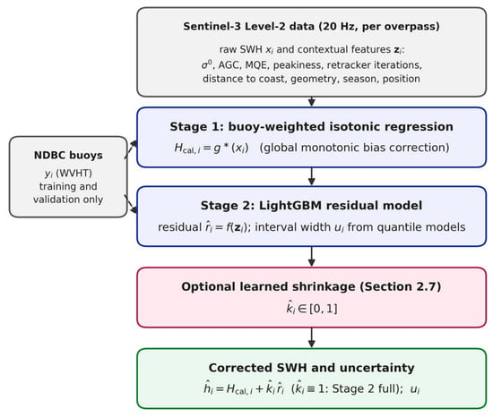
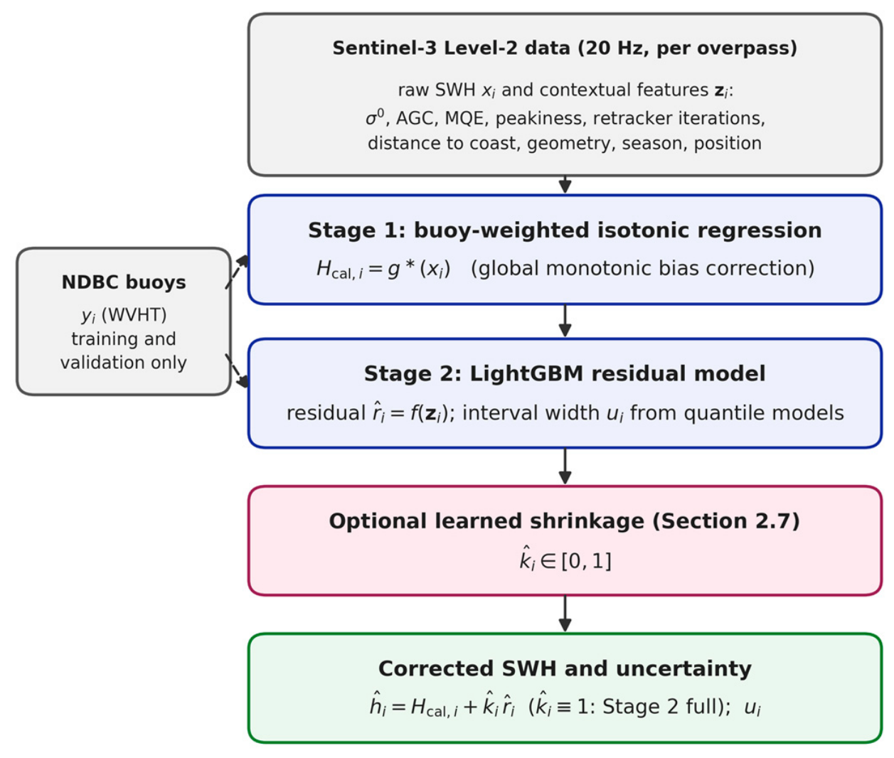
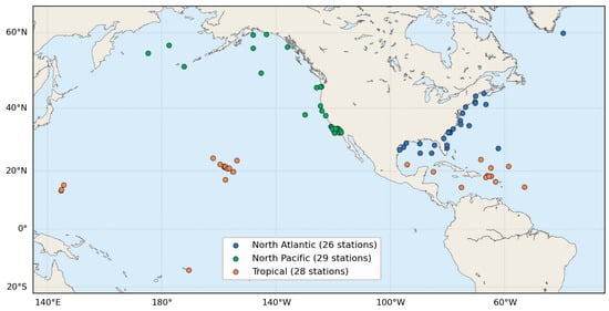
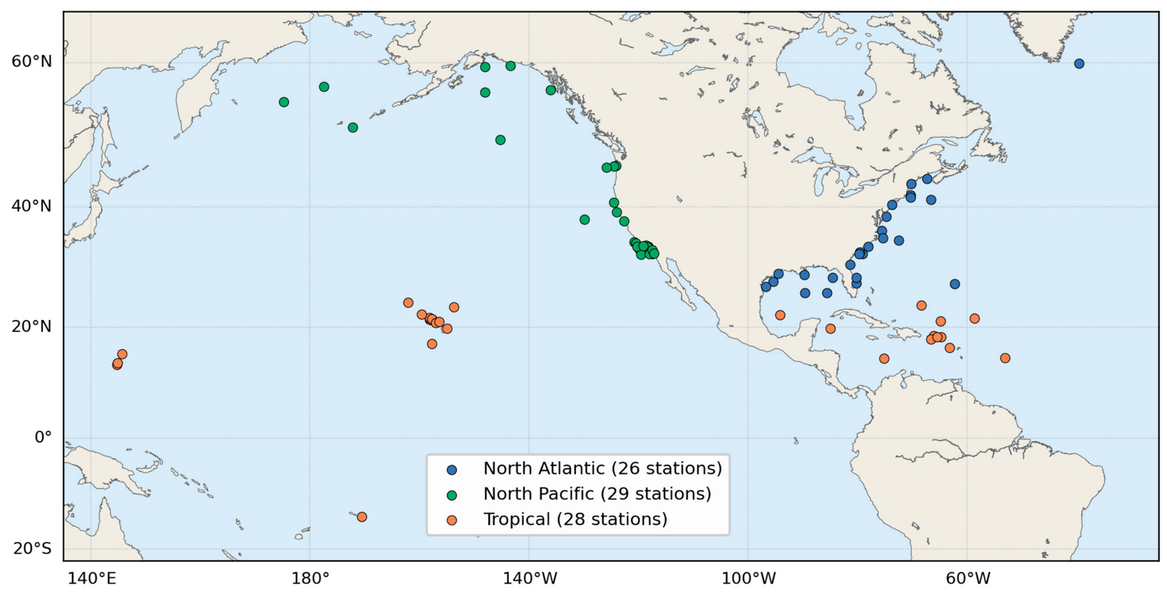
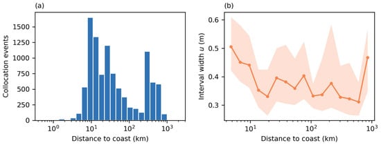
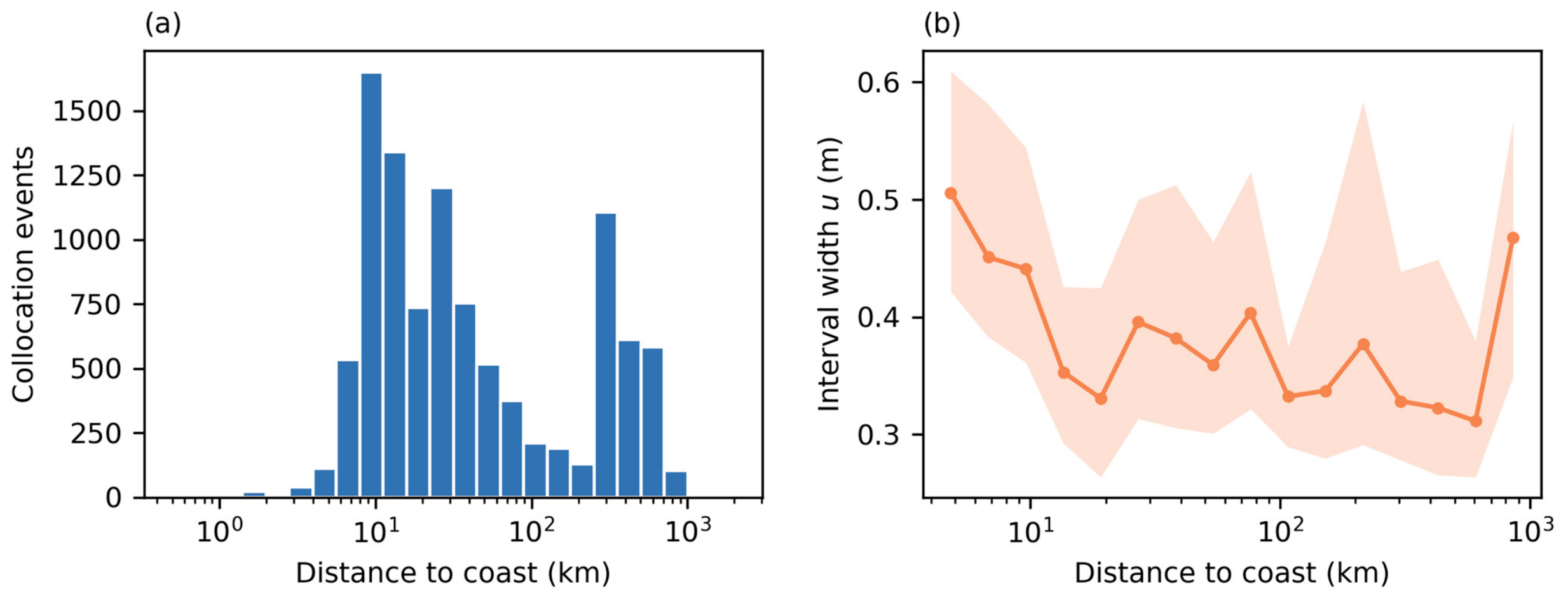
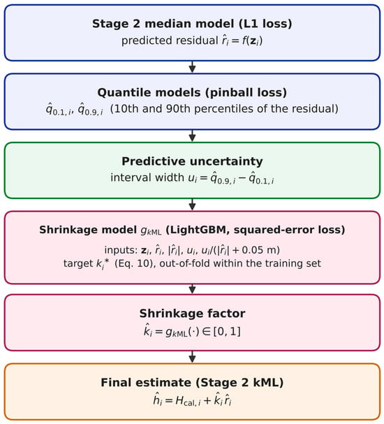
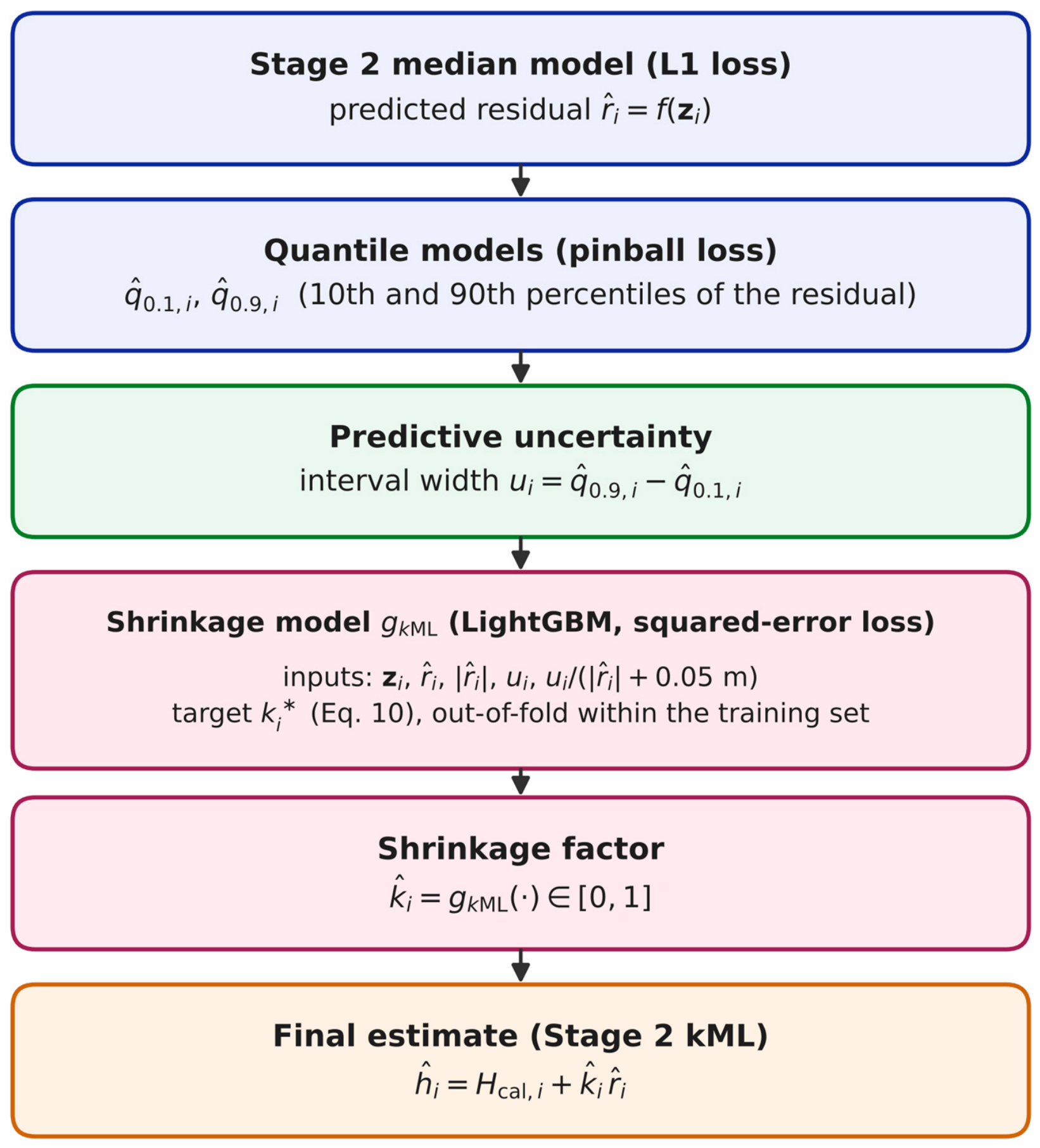
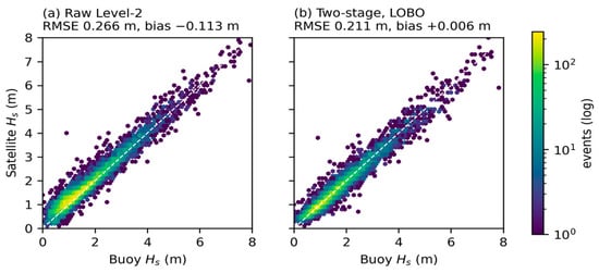
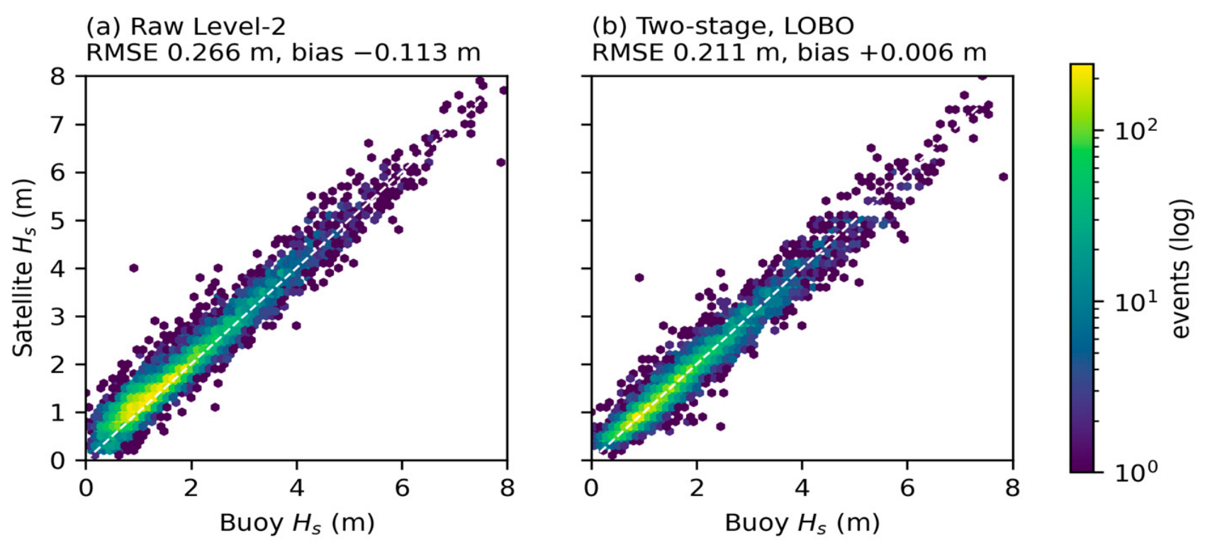
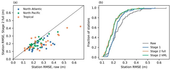
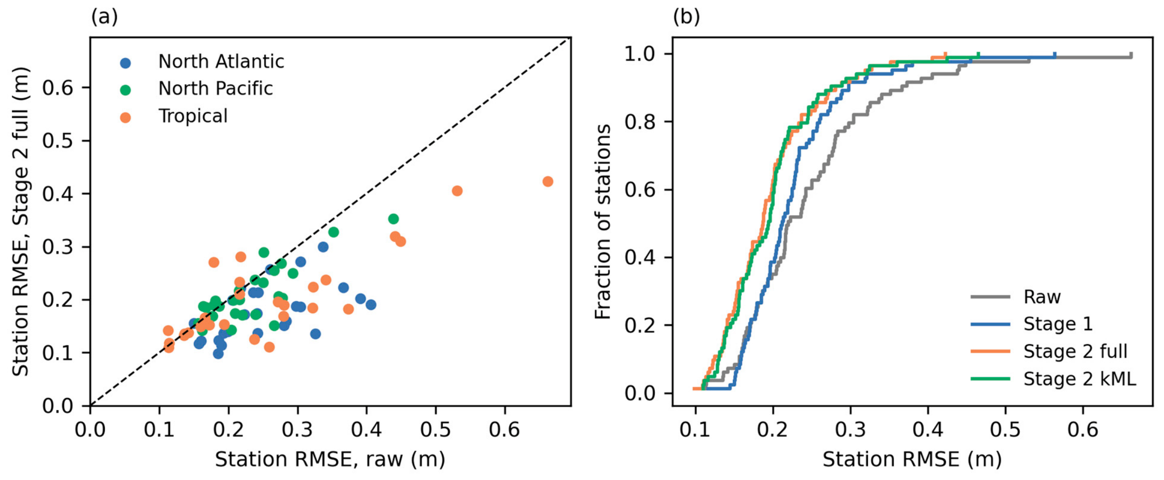
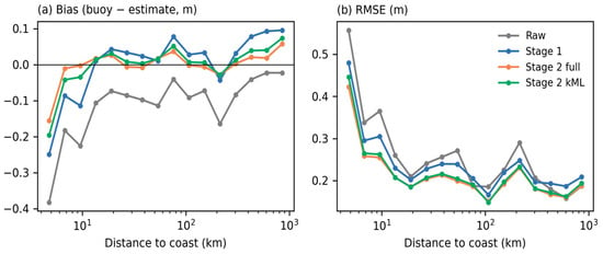
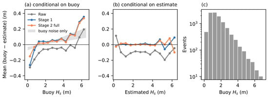
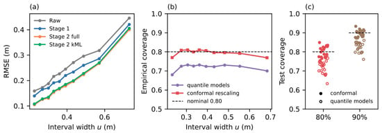
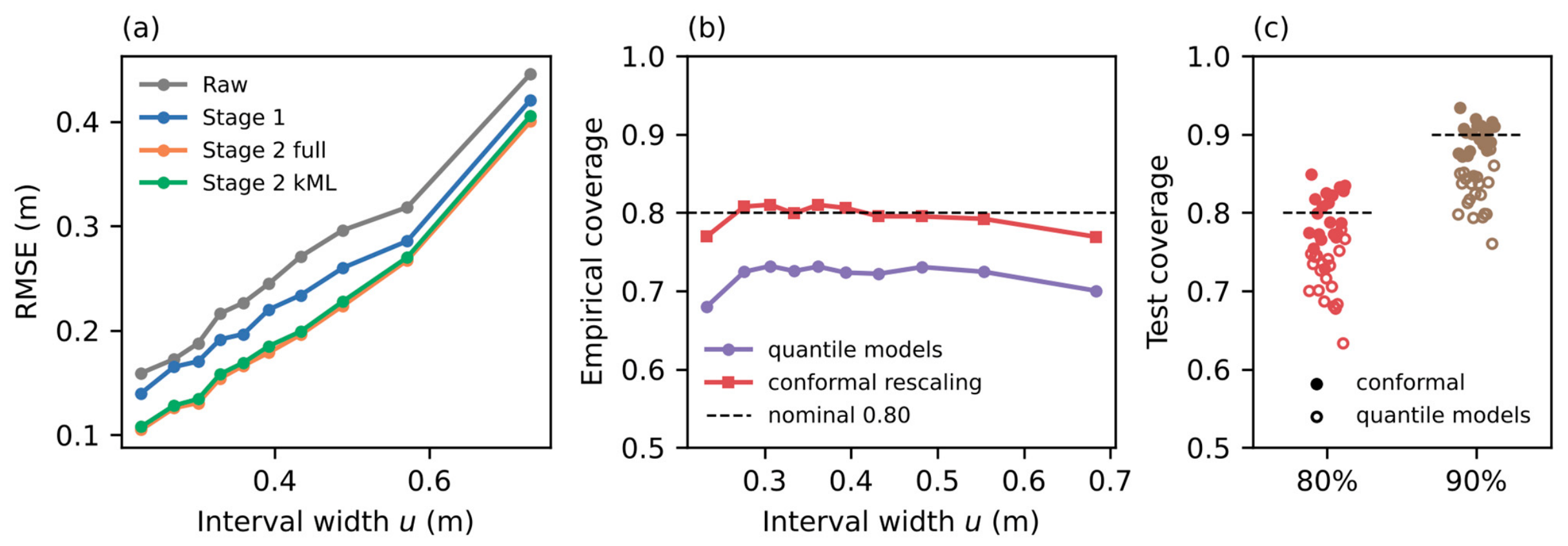
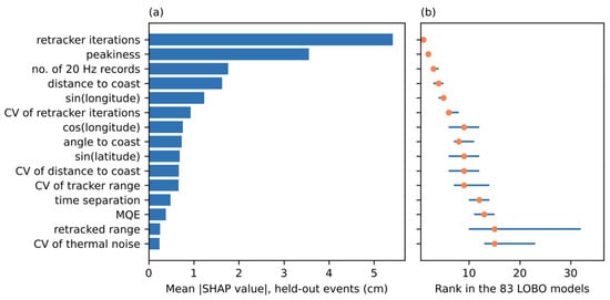
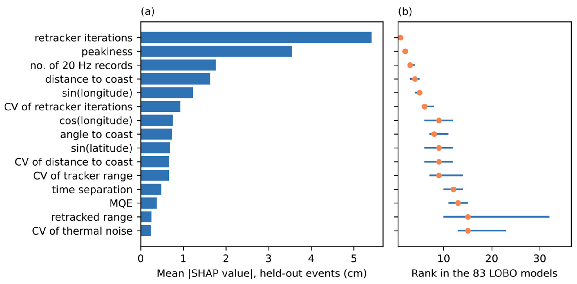

Disclaimer/Publisher’s Note: The statements, opinions and data contained in all publications are solely those of the individual author(s) and contributor(s) and not of MDPI and/or the editor(s). MDPI and/or the editor(s) disclaim responsibility for any injury to people or property resulting from any ideas, methods, instructions or products referred to in the content. |
© 2026 by the authors. Licensee MDPI, Basel, Switzerland. This article is an open access article distributed under the terms and conditions of the Creative Commons Attribution (CC BY) license.