A Method for Estimating Global Sectional Loads from Local Point Strain Monitored on Real Ship Hull Structures

Abstract

The real-time monitoring of global sectional loads is crucial for the safety assessment of ship hulls during operation, yet it remains a significant challenge due to the complexity of the structure and the marine environment. Direct measurement of hull global sectional loads remains difficult in practical engineering, whereas local strain responses can be conveniently obtained using strain gauge. This paper presents an analytical physics-driven load conversion framework to reconstruct global sectional load components from limited longitudinal strain measurements for full-scale ship hull structures. A load conversion matrix is established based on a linear superposition of strain components from vertical bending, horizontal bending, axial force, and warping torsion. The method is first validated on a simplified U-shaped beam using finite element analysis, identifying optimal sensor arrangements. It is then extended to a uniform beam with the complex midship section of a 21,000 TEU containership, where its accuracy is further confirmed under both static and dynamic periodic loading conditions. Finally, the proposed method is validated against CFD-FEM coupled simulation results for the containership under regular head waves and oblique short-crested irregular waves. This study provides a feasible analytical tool for reconstructing hull girder sectional loads using sparse local strain monitoring data, which can be used in applications such as full-scale ship structural health monitoring and global strength assessment.

1. Introduction

As a vital means of maritime transportation, ships play an irreplaceable role in global cargo logistics and naval operations. However, hull structures are persistently subjected to time-varying dynamic wave loads in complex oceanic environments [1,2,3]. Global sectional loads, including vertical bending moment (VBM), horizontal bending moment (HBM), torsional moment (TM) and shear forces, are critical throughout the entire service life of a ship. At the design stage, these sectional loads serve as fundamental criteria for determining structural scantlings. During real-world operation, real-time sectional load information underpins ship structural health monitoring [4,5,6], enabling onboard safety evaluation and early warning against extreme sea events. Consequently, global sectional loads constitute not only essential prerequisites for ship design but also core inputs for intelligent navigation decision-making and maritime risk management.

A wide spectrum of techniques has been developed to evaluate ship sectional loads under various sea states. Representative approaches include the rule books of classification societies [7], empirical formulations [8], potential flow-based numerical calculations [9], computational fluid dynamics (CFD) simulations [10,11] and model experiments [12,13,14]. For instance, Vijith et al. [15] predicted rigid bending and torsional loads on large slender ships based on strip theory. Zhang et al. [16] employed a coupled CFD-MBD framework to compute VBM for a 20,000 TEU containership. Chen et al. [17] carried out CFD-FEM co-simulations to obtain sectional loads of a whole-ship structure in short-crested waves. Meanwhile, experimental investigations are commonly conducted using segmented ship models in wave tanks. For example, Chen et al. [18] explored how segment quantity influences higher-order sectional load components. Furthermore, large-scale model experiments can be employed for near-shore sea trials, through which hull sectional loads under realistic wave conditions can be acquired [19,20,21]. To conclude, these forward prediction methods facilitate the estimation of ship loads during the design stage or under specific conditions, primarily relying on specially designed models.

In practical engineering applications, direct measurement of global sectional loads onboard full-scale ships remains infeasible. Instead, sectional loads must be inferred indirectly from measured stress or strain responses. For segmented experimental ship models, strain gauges mounted on simple, uniform backbone beams (e.g., hollow circular or rectangular cross-sections) allow sectional loads to be extracted via full-bridge circuits. However, such beam sections are too simple to reflect full-scale real ship structures. A flexible monoblock model is made of special elastic materials, and both the whole structure and local structures of the ship model are considered [22,23]. For example, Grammatikopoulos et al. [24] designed and made a fully elastic model of a uniform containership with the help of 3D printing. The design, construction and testing of a fully elastic ship model for investigating hydroelastic responses of containerships are reported in Chen et al. [25]. For complex built-up cross-sections, a straightforward simple beam bending formula $M_y={\displaystyle \frac{\sigma I_y}{z}}$ has considerable limitations. Moreover, the vast majority of the literature uses a Timoshenko or Vlasov beam approximation for beams [26,27]. For instance, Zhou et al. [28] predicted the ship hydroelastic responses using Timoshenko beam modes. Nevertheless, a few existing studies still rely on this simplified beam hypothesis for load estimation due to its computational convenience, which is applicable under static or quasi-static conditions. For example, Prini et al. [29] estimated global hull loads from stress measurements obtained during full-scale sea trials of a lifeboat using simplified beam theory.

Nowadays, stress/strain monitoring systems have become mature, offering high measurement precision, high sampling rates, compact hardware forms and convenient installation across various fields [30,31,32,33]. Such integrated systems support data acquisition, storage and post-processing. Strain sensors, as core components of these monitoring systems, are widely employed for local structural monitoring on ships [6,34]. For example, Komoriyama et al. [35] used fibre-Bragg-grating sensors to evaluate hull girder strength and validated the results through experiments in the towing tank. Zheng et al. [36] assessed the structural safety of ships and offshore platforms based on strain-sensor measurements. In these prior works, local stress/strain data were mainly utilized to evaluate local structural strength and fatigue performance, rather than to recover global hull girder sectional loads. The main reason is that sectional loads cannot be reliably reconstructed solely from the local stress of one point.

Determining unknown external loads from measured structural responses under excitation represents a classic inverse engineering problem known as load identification or load inversion [37,38]. This technique solves the input-output relationship of a structural system inversely, delivering an indirect pathway to obtain loads that are physically difficult to measure directly. Given the clear physical linkage between strain and internal force, local strain measurements are frequently adopted as input data for load inversion. Zheng et al. [39] proposed a method to identify the random fluctuating pressure on a structure from monitored strain in three directions (ε_x, ε_y, τ_xy) via strain gauges. Guo et al. [40] implemented real-time Bayesian axial load identification for track and bridges from flexural strain signals. Sha et al. [41] performed load inversion for jacket offshore platforms by assuming measured uniaxial strain as the linear superposition of contributions from multiple load components.

Existing load inversion approaches can be categorized into data-driven methods and physics-model-driven methods. The former learns implicit input-output mappings from large-volume datasets without explicit physical governing equations. Typical techniques include artificial neural networks and various deep learning methods [42,43,44]. Zhang et al. [45] applied a load inversion method based on deep learning to obtain real-time wind loads for two skyscrapers in China. Jia et al. [46] compared three ensemble learning models (Extra Trees, AdaBoost, LightGBM) for load inversion on offshore platforms. Wan et al. [47] identified random dynamic structural loads for rocket mock-up cabins using long short-term memory (LSTM) networks. However, data-driven inversion strongly depends on abundant, high-quality training datasets. When dealing with new conditions outside the training set, prediction accuracy degrades. Additionally, these black-box models lack physical interpretability.

By contrast, physics-model-driven methods exploit explicit mathematical and mechanical relationships to achieve load inversion [48,49]. These methods provide good interpretability, robustness and high accuracy, while imposing relatively low requirements on data quantity. Dui et al. [50] proposed a stepwise method based on Schmidt’s orthogonalization of the maximum vertical distance, to invert wing load rams of an aircraft under fatigue conditions. Guo et al. [51] identified aerodynamic pressure loads on a three-dimensional (3D) wing structure by combining surface flattening and subregion interpolation. Zareei et al. [52] developed a state-space load identification approach based on the balancing principle, which identified the grounding impact loads of the ship-stiffened panels. Overall, load inversion methods have been widely investigated and validated in engineering practice across various fields.

Despite these advances in load identification, there remains a lack of engineering methodologies that can robustly reconstruct sectional loads for large ships using minimal, real-time response data. Most published research still concentrates on forward prediction or localized structural monitoring. Another obstacle restricting the development of ship sectional load conversion is the difficulty of acquiring benchmark sectional load data from full-scale sea trials for validation purposes. Recent progress in high-fidelity numerical wave tank technology enables CFD-FEM two-way coupled simulations to output both detailed hull stress distributions and global sectional load time series data [53,54,55,56], which can be used for validation of the sectional load conversion method.

Against this background, the present paper proposes an analytical load- conversion framework for full-scale ship structural monitoring, using real-time longitudinal strain measurements. Section 2 derives a load conversion matrix that accounts for warping effects (Vlasov beam) induced by restrained torsion. The target ship structure and design loads are described in Section 3. Section 4 and Section 5 validate the proposed approach under static and dynamic loading conditions, employing simplified U-shaped beams and beam models built from a real-ship midship cross-section, respectively. Subsequently, the method is applied to reconstruct real-time sectional loads for a full-scale whole-ship containership structure under oceanic wave environments. This work offers technical insights for sectional load conversion within structural health monitoring for seagoing ships.

2. Sectional Load Conversion Method

It is important to obtain global sectional loads on the hull structures of real ships sailing in waves, which is widely applicable for comparison with or validation of sectional loads obtained from classification society rules, direct calculations based on potential flow theory or tank model experiments. Moreover, one of the main objectives of structural health monitoring (SHM) is to assess structural stress states and provide safety alerts by continuously collecting relevant data through onboard measurement sensors.

In this section, a strain-based load conversion method is proposed, which offers general applicability to slender beam structures such as ship hulls, long-span bridges, wind turbine towers, long-distance pipelines, and railway tracks. By strategically arranging strain sensors at critical cross-sections and establishing a mechanical mapping relationship between measured local stresses and sectional loads, it is possible to extrapolate the dynamic sectional loads from real-time local stress data. This, in turn, provides crucial support for informed safety assessments and timely early warning decisions, especially for SHM systems.

2.1. Problem Statement

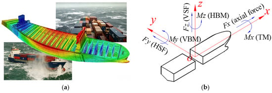
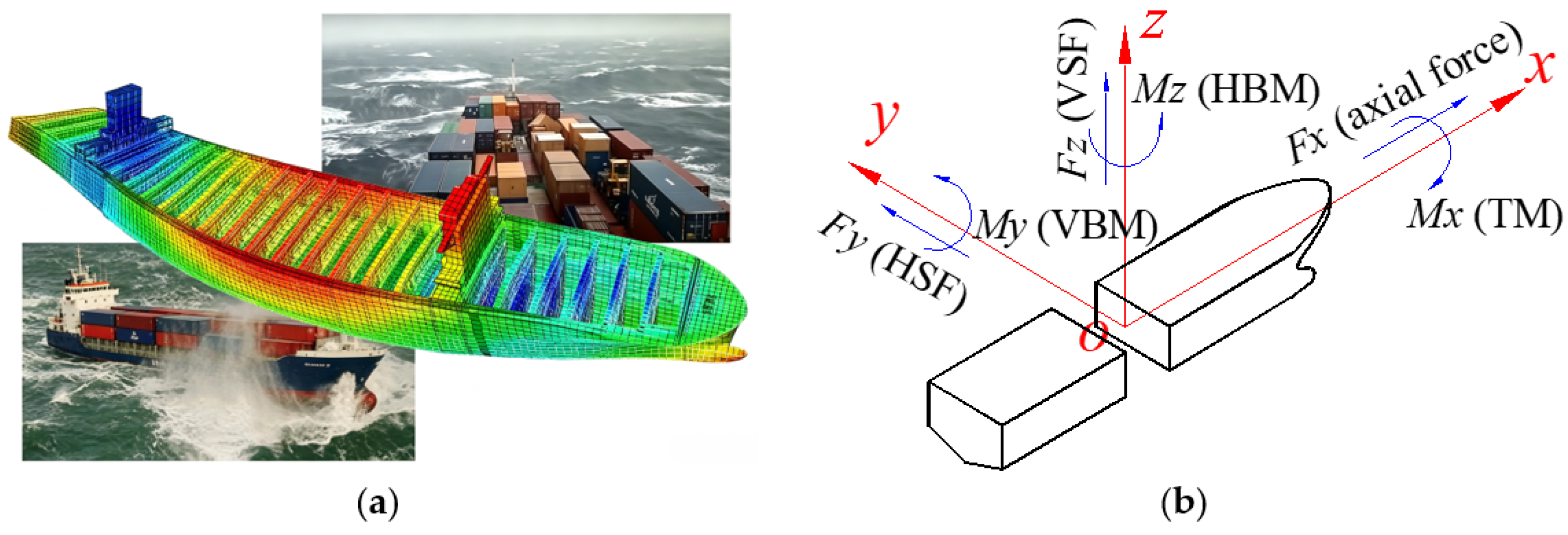
Modern ocean-going ships are developing towards lighter and larger designs, with length-to-width and length-to-depth ratios ranging from 8 to 12. During ship navigation at sea, environmental factors such as wind, waves and currents, as well as the propulsion system, induce complex hull structural loads. As shown in Figure 1, the global sectional loads include three forces, i.e., the axial force F_x, the horizontal shearing force (HSF) F_y, the vertical shearing force (VSF) F_z, and three moments, i.e., the vertical bending moment (VBM) M_y, the horizontal bending moment (HBM) M_z and the torsional moment (TM) M_x. For a real ship sailing in ocean waves, the six force/moment components exist simultaneously. Due to the complexity of the ocean environment and real ship structures, the sectional loads are difficult to measure directly.

Figure 1. Ship local and global structural loads in sea waves. (a) Ship structural stress distribution in waves. (b) Sectional loads on ship hull structure.

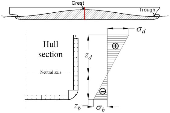
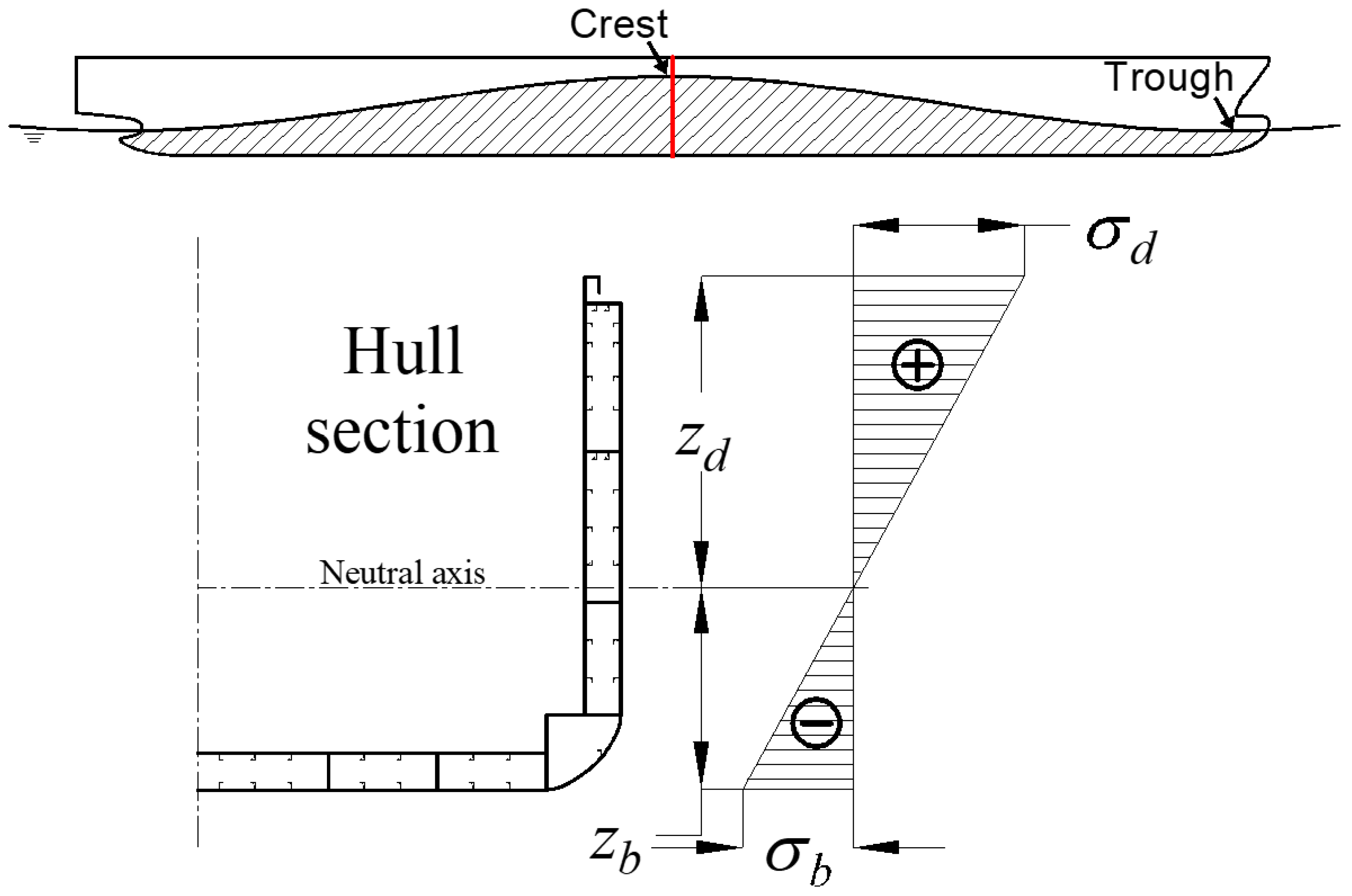
The VBM is one of the greatest concern among all six sectional loads. The traditional method for estimating the VBM is the use of simple beam theory. As shown in Figure 2, the hogging VBM (M_y) on a ship section can be estimated by:

$$M_y={\displaystyle \frac{\sigma \cdot I}{z}}=\sigma \cdot W$$

(1)

where σ represents the longitudinal stress at a specific point, I represents the moment of inertia of the section about the neutral axis, z represents the vertical distance between the stress measuring position and the neutral axis, and W represents the section modulus.

Figure 2. Description of the longitudinal stress on the ship hull section due to VBM.

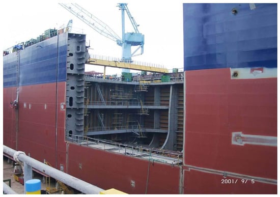
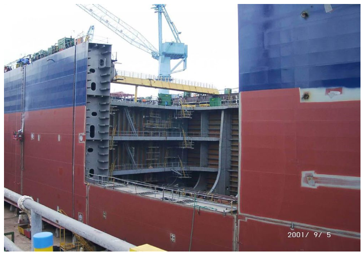
However, this is accurate only when pure bending occurs on the ship hull. In fact, the real hull structure is complex and comprises components such as inner plates, ribs, stiffeners and transverse bulkhead, as depicted in Figure 3. Local stress results from the combined contributions of all six sectional loads. For a real ship operating in ocean waves, bending, tensile and warping deformations occur at the same time. It is not possible to accurately estimate the VBM based on stress at a single position. With this in mind, the strain-based load conversion method is proposed in this paper to obtain VBM and HBM, which is essential for the real-time assessment of ship structural safety. This method can also be extended for load conversion and estimation for other beam-like engineering structures.

Figure 3. Example of the complex internal structure arrangement of a real containership.

2.2. Local Stress Calculation Formulation

The longitudinal stress on the ship hull surface is mainly caused by the contributions of VBM, HBM, axial force and torsional moment. This section describes the relationship between longitudinal stress and each of the sectional loads.

(1)

Bending moment-induced longitudinal strain

With the assumption of pure bending, the ship hull is considered to be subjected exclusively to vertical or horizontal bending moments, while the effects of torsional moments and shear deformations are neglected [57]. With the coordinate origin positioned at the vertical neutral axis of the ship’s cross-section, the longitudinal strain ε_a at any measurement point (y, z) can be obtained from the sum of the vertical and horizontal bending moments, which is described as:

$${\epsilon }_a={\displaystyle \frac{M_y\cdot z}{E{I}_y}}+{\displaystyle \frac{M_z\cdot y}{E{I}_z}}$$

(2)

where M_y and M_z represent the VBM and HBM, respectively, E represents the elastic modulus, and I_y and I_z represent the moments of inertia of the transverse section about the y-axis and z-axis, respectively.

(2)

Axial force-induced longitudinal strain

Under the assumption of pure axial loading, the ship hull is subjected exclusively to tension or compression. In this state, localized complex stress states arising from the Poisson effect are disregarded to maintain a simplified uniaxial response [58]. Consequently, the relation between the longitudinal strain ε_b at a measuring point and the axial force is described as:

$${\epsilon }_b={\displaystyle \frac{F_x}{E\cdot A}}$$

(3)

where F_x represents the axial force (positive for tension, negative for compression), and A represents the cross-sectional area of the structure.

(3)

Secondary torsional moment-induced longitudinal strain

When structural deformation occurs in a uniform cylindrical structure under a free torsional moment, the axial displacements on the cross-section are identical, which means that warping deformation does not occur in the cross-section. Thus, there is no longitudinal stress arising from warping in this case. For thin-walled beams, longitudinal stress induced by free torsion is ignored in this paper. However, restrained torsion arises when warping deformation is obstructed by end constraints, cross-sectional variations, or non-uniform torsional loading [59]. Unlike free torsion, the axial gradient of warping in restrained torsion generates non-uniform, self-equilibrating longitudinal normal stresses. To satisfy equilibrium, a secondary shear flow is induced in addition to the traditional St. Venant shear flow [60].

The secondary flow contributes an additional torsional component, which is termed the secondary (warping) torsional moment. Thus, the total torsional moment is the summation of the free and secondary torsional moments. This stress state is formulated using the bimoment as follows [61].

$$T_w={\displaystyle \frac{\mathit{dB}}{\mathit{dx}}}$$

(4)

where T_w represents the secondary torsional moment, and B is the bimoment.

Assume that the thin-walled beam is subjected exclusively to restrained torsion, with the structural response driven by the secondary torsional moment. The relationship between the sectional bimoment and the longitudinal strain ε_c induced by it at the measuring point is given as [62]:

$${\epsilon }_c={\displaystyle \frac{\mathit{Bw}}{E{I}_w}}$$

(5)

where w represents the sectorial coordinate at the measuring point, and I_w represents the sectorial moment of inertia of the cross-section.

The sectorial coordinates for all nodes on the cross-section can be calculated as follows [62]:

$${\left[K_w\right]}_{N_P\times N_P}\cdot {\left[w\right]}_{N_P\times 1}={\left[Q\right]}_{N_P\times 1}$$

(6)

where N_P represents the number of nodes.

The elements in the coefficient matrix ${\left[K_w\right]}_{N_P\times N_P}$ are obtained as follows:

$$k_{\mathit{ii}}={\displaystyle {\sum }_i^{(1)}\frac{t}{l}}+{\displaystyle {\sum }_i^{(2)}\frac{t}{l}},i=1,2\dots N_{P-1}$$

(7)

$$k_{\mathit{ij}}=-{\displaystyle \frac{t_{\mathit{ij}}}{l_{\mathit{ij}}}},i=1,2\dots N_{P-1},j\ne i$$

(8)

$$k_{N_{P}j}={\displaystyle {\sum }_j\mathit{lt}},\mathrm{j}=i=1,2\dots N_P$$

(9)

where ${\displaystyle {\sum }_i^{(1)}}$ represents the sum of all elements starting from node i, ${\displaystyle {\sum }_i^{(2)}}$ represents the sum of all elements ending at node i, t represents the element plate thickness, and l represents the element length.

The elements in vector ${\left[Q\right]}_{N_P}$ are obtained as follows:

$$q_i={\displaystyle {\sum }_i^{(2)}\mathit{th}}-{\displaystyle {\sum }_i^{(1)}\mathit{th}},i=1,2\dots N_{P-1}$$

(10)

$$q_{N_P}=0$$

(11)

where h represents the vertical distance between the element centerline and the shear center. The parameter h is taken to be positive when the radius vector from the shear center to the element midline rotates clockwise during traversal from the starting to the ending node. Conversely, counterclockwise rotation indicates a negative value.

2.3. Local Conversion Matrix

A beam-like ship structure can be idealized as a slender thin-walled beam. The hull girder beam can be either open or close. For example, the cross-section of containership with large deck opening is considered as U-shaped. For a beam structure, the longitudinal strain at any specified point can be regarded as the linear superposition of longitudinal strain components caused by sectional bending moments, axial force and secondary torsional moment due to environmental loads. Since there are four kinds of unknown load components in each equation, four equations should be used to solve the unknown quantities. Therefore, the longitudinal strain of at least four points should be used as input. By combining Equations (2), (3) and (5), the relation between ship global sectional loads and local longitudinal strains at any cross-section can be expressed as [63,64]:

$$\left[\begin{array}{c}{\epsilon }_1\\ {\epsilon }_2\\ {\epsilon }_3\\ {\epsilon }_4\end{array}\right]=\left[\begin{array}{cccc}{\displaystyle \frac{z_1}{E{I}_y}}& {\displaystyle \frac{y_1}{E{I}_z}}& {\displaystyle \frac{1}{\mathit{EA}}}& {\displaystyle \frac{w_1}{E{I}_w}}\\ {\displaystyle \frac{z_2}{E{I}_y}}& {\displaystyle \frac{y_2}{E{I}_z}}& {\displaystyle \frac{1}{\mathit{EA}}}& {\displaystyle \frac{w_2}{E{I}_w}}\\ {\displaystyle \frac{z_3}{E{I}_y}}& {\displaystyle \frac{y_3}{E{I}_z}}& {\displaystyle \frac{1}{\mathit{EA}}}& {\displaystyle \frac{w_3}{E{I}_w}}\\ {\displaystyle \frac{z_4}{E{I}_y}}& {\displaystyle \frac{y_4}{E{I}_z}}& {\displaystyle \frac{1}{\mathit{EA}}}& {\displaystyle \frac{w_4}{E{I}_w}}\end{array}\right]\cdot \left[\begin{array}{c}{M}_y\\ M_x\\ F_x\\ B\end{array}\right]$$

(12)

where the left side of the equation is the strain matrix, and the right side is the dot product of the stiffness matrix and the sectional load matrix. Conversely, the ship sectional loads at any arbitrary station can be calculated from the longitudinal strains monitored at a minimum of four points.

$$\left[\begin{array}{c}{M}_y\\ M_z\\ F_x\\ B\end{array}\right]={\left[\begin{array}{cccc}{\displaystyle \frac{z_1}{E{I}_y}}& {\displaystyle \frac{y_1}{E{I}_z}}& {\displaystyle \frac{1}{\mathit{EA}}}& {\displaystyle \frac{w_1}{E{I}_w}}\\ {\displaystyle \frac{z_2}{E{I}_y}}& {\displaystyle \frac{y_2}{E{I}_z}}& {\displaystyle \frac{1}{\mathit{EA}}}& {\displaystyle \frac{w_2}{E{I}_w}}\\ {\displaystyle \frac{z_3}{E{I}_y}}& {\displaystyle \frac{y_3}{E{I}_z}}& {\displaystyle \frac{1}{\mathit{EA}}}& {\displaystyle \frac{w_3}{E{I}_w}}\\ {\displaystyle \frac{z_4}{E{I}_y}}& {\displaystyle \frac{y_4}{E{I}_z}}& {\displaystyle \frac{1}{\mathit{EA}}}& {\displaystyle \frac{w_4}{E{I}_w}}\end{array}\right]}^{-1}\cdot \left[\begin{array}{c}{\epsilon }_1\\ {\epsilon }_2\\ {\epsilon }_3\\ {\epsilon }_4\end{array}\right]$$

(13)

2.4. Calculation Process and Validation Procedure

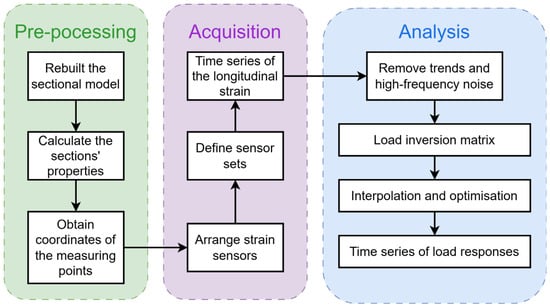
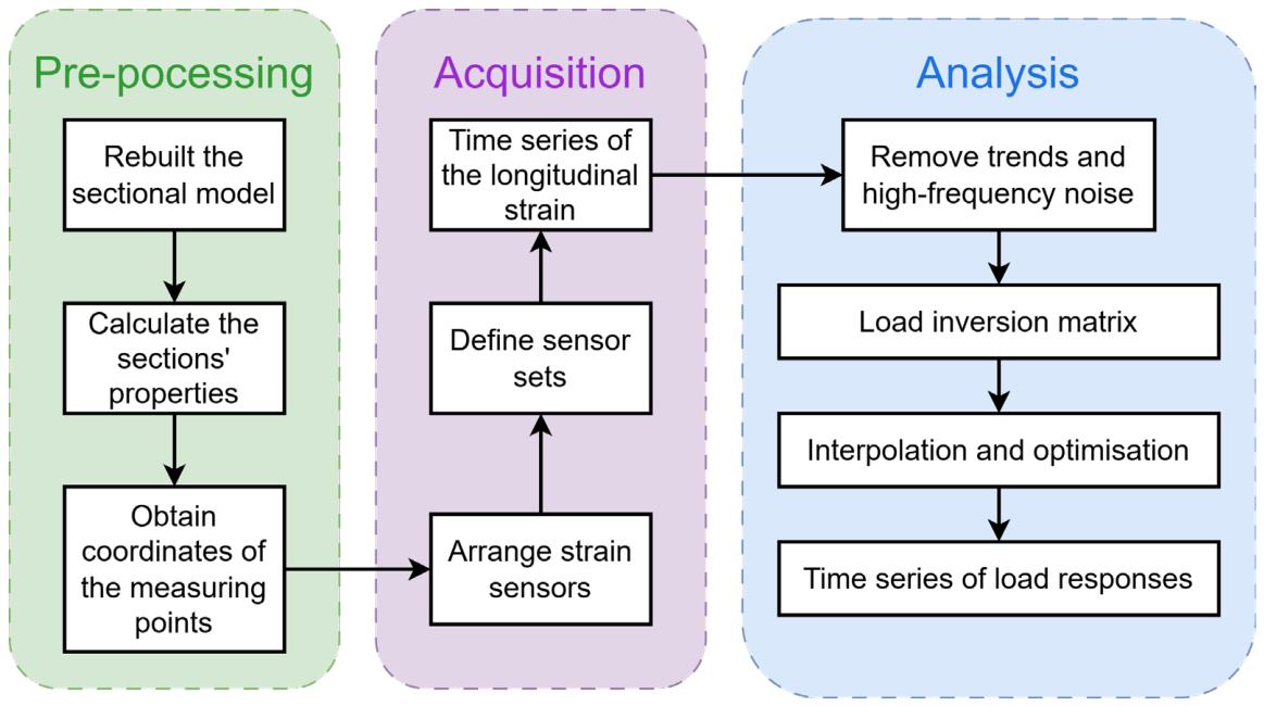
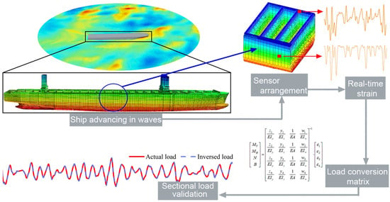
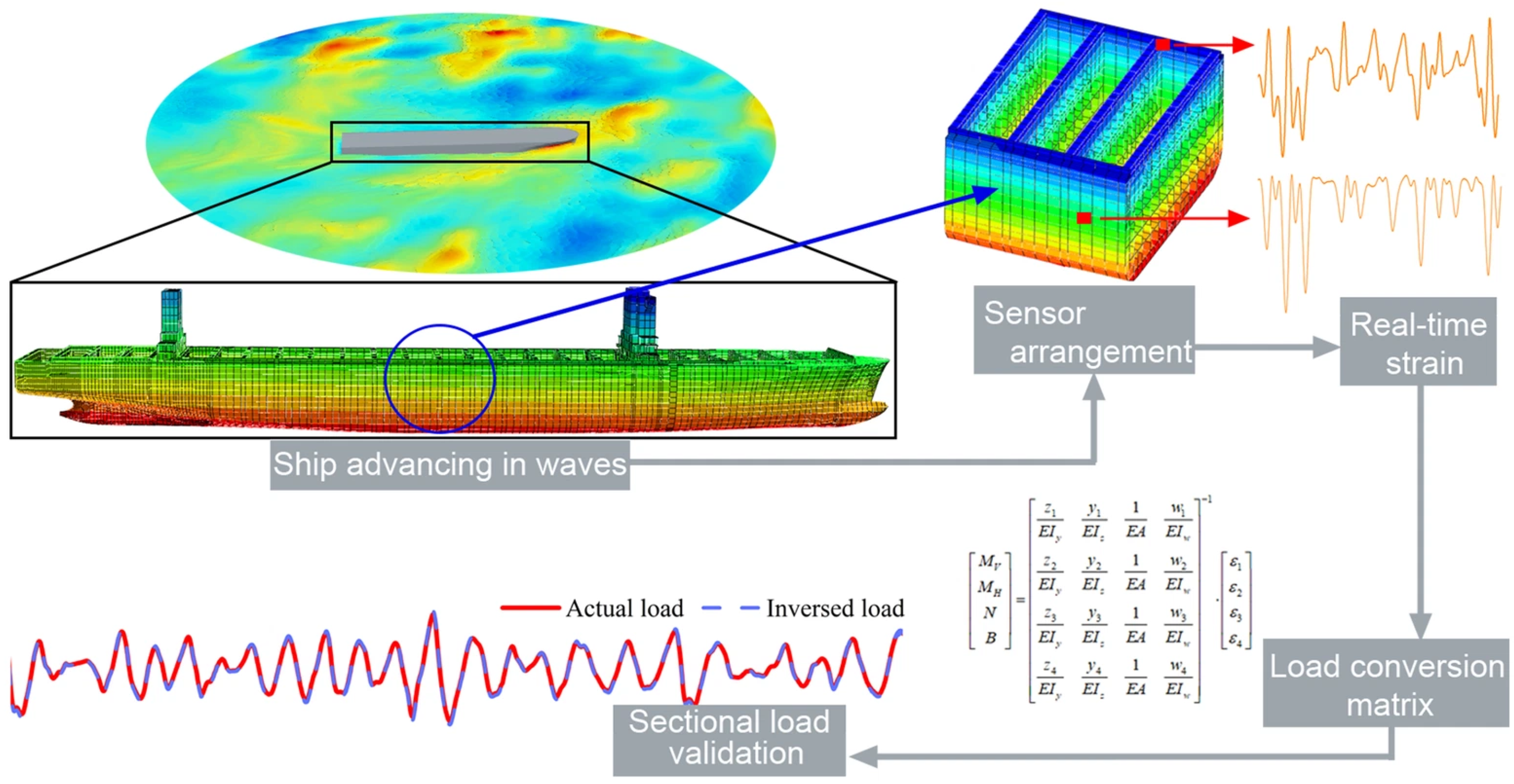
According to the load conversion matrix, load conversion can be applied to the ships operating at sea. Figure 4 gives a flowchart for the process of ship load conversion. Three main stages are included. Specifically, in the pre-processing stage, due to the structural complexity of actual ship structures, the target cross-section should be idealized and simplified. The simplification follows rules such as approximating curved geometries with linear segments and modeling secondary structural components as lumped sectional areas. Furthermore, to obtain the sectorial coordinate of the measuring sensors, element nodes should be set to coincide with the exact locations of the sensors. The section properties, including cross-sectional area, moment of inertia, positions of the center of gravity and shear center, are calculated based on the rebuilt sections. In the analytical stage, sectional loads are converted according to Equation (13).

Figure 4. Workflow of ship sectional load conversion.

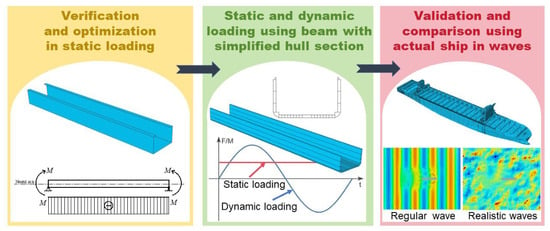
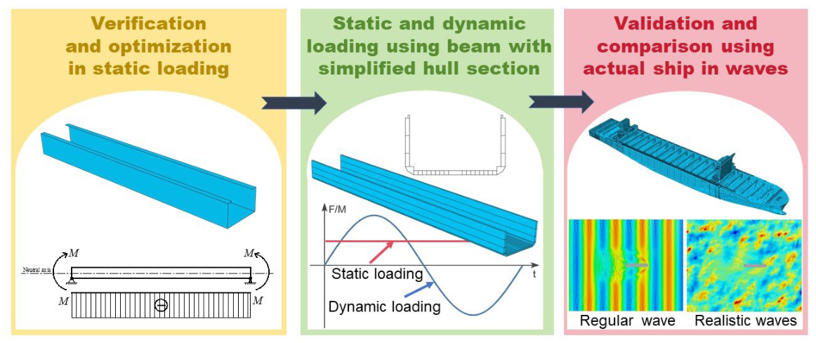
The ultimate objective of this study is to estimate the sectional loads on a real ship’s structure sailing in realistic ocean waves by using the developed method. A 21,000 TEU containership is used as the target ship for this study. Figure 5 presents the verification and validation process for the proposed load conversion method, which includes three main steps.

Figure 5. Verification and validation process for the proposed load conversion method.

First, a simplified U-shaped uniform beam is used to preliminarily verify the method. The simplified U-shaped beam’s cross-section is designed to have the same vertical and horizontal moments of inertia as the midship section of the target containership. The beam length is the same as the full-scale ship length. External static loads such as axial force, bending moment and torsional moment, either independently or in combination, with specified magnitudes are applied to the beam. The longitudinal strains monitored at typical positions are used as inputs for the sectional load conversion calculation, and the results are subsequently validated against the target values. Moreover, the influence of location and number of strain monitor points on the estimation results is studied.

Then, a uniform beam with the real ship’s cross-section is used to further verify the method. Both specified static and dynamic periodic loads are applied to the beam for study and validation. The estimated sectional loads and the known applied loads are compared to extend the effectiveness of the method to complex structures and complex dynamic loading conditions.

Finally, the developed method is applied to the whole-ship structure of a 21,000 TEU containership sailing in ocean waves. A CFD-FEM two-way coupled method is used to simulate the time series of loads of the ship under regular head waves [55,56] and oblique short-crested irregular waves [17,53,54]. The estimated sectional loads are compared with the numerical simulation results to demonstrate the practical applicability of the developed method.

3. Target Ship Structure and Design Loads

3.1. Containership Hull Structure

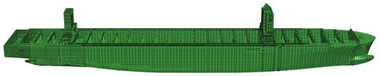
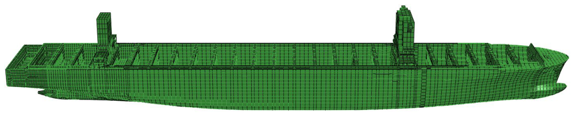
A 21,000 TEU containership is used as the target ship in this study. Main dimensions of the containership are listed in Table 1. The whole-ship structural finite element (FE) model, which was initially modeled by MSC.Patran, is shown in Figure 6. The FE model includes all the local structural details of a real ship, such as plates, girders and bones. The structural model has the material property of the high-strength steel.

Table 1. Main dimensions of the 21,000 TEU containership.

Item	Value
Length overall, L (m)	400
Length between perpendiculars, Lpp (m)	386
Breadth, B (m)	58.6
Depth, D (m)	33.5
Draft, T (m)	16
Displacement, ∆ (ton)	260,401
Block coefficient, CB	0.6164
Waterplane area coefficient, CW	0.876

Figure 6. Whole-ship structural FE model of a 21,000 TEU containership.

3.2. Determination of Design Loads

External loads acting on a real containership should be estimated to reflect the magnitude of design loads. Thus, they are calculated according to the rules of the China Classification Society [7] or empirical formulas.

The external axial force is determined based on the ship’s resistance at the design speed (V = 22 kn). Total resistance can be calculated as follows:

$$R_T={\displaystyle \frac{1}{2}}\mathit{\rho S}{V}^2{C}_T$$

(14)

where ρ represents the density of seawater, and S represents the wetted surface area, calculated as:

$$S=L_{\mathit{PP}}(2T+B)\sqrt{C_B}$$

(15)

The total resistance coefficient C_T can be calculated as follows:

C_T = C_F(1 + k) + C_W + C_A

(16)

where C_F, k, C_W and C_A are the frictional resistance coefficient, form factor, wave-making resistance coefficient and correlation allowance, and in this study, they are set to 0.00078, 1.18, 0.00024 and 0.00013, respectively.

The VBM of the containership at any longitudinal section can be calculated as follows:

M_y = 9.81MKFL²B(C_B + 0.7) × 10⁻² kN ⋅ m

(17)

where M represents the VBM distributed factor, and K and F are coefficients, which can be calculated as follows:

$$M=\left\{\begin{array}{c}{\displaystyle \frac{x}{4L}},0\le {\displaystyle \frac{x}{L}}\le 0.4\\ 1,0.4<{\displaystyle \frac{x}{L}}<0.65\\ -{\displaystyle \frac{20x}{7L}}+{\displaystyle \frac{20}{7}},0.65\le {\displaystyle \frac{x}{L}}\le 1\end{array}\right.$$

(18)

$$K=4.47{\left({\displaystyle \frac{L}{1000}}-0.23\right)}^2+0.817$$

(19)

$$F=9.4-0.45{\left({\displaystyle \frac{L-350}{100}}\right)}^{{\displaystyle \frac{3}{2}}}$$

(20)

where x represents the distance from the calculation section to the aft perpendicular.

The HBM of the containership at any section can be calculated as follows:

M_z = 0.431L²Bk kN ⋅ m

(21)

where k represents the HBM distributed factor and can be calculated as follows:

$$k=\left\{\begin{array}{c}{\displaystyle \frac{2x}{L}},0\le {\displaystyle \frac{x}{L}}\le 0.5\\ -{\displaystyle \frac{2x}{L}}+2,0.5<{\displaystyle \frac{x}{L}}\le 1\end{array}\right.$$

(22)

The TM of the containership at any section can be calculated as follows:

$$M_x\left(x\right)=9.81e^{-0.00295L}{\displaystyle \frac{L{B}^3{C}_T}{100}}\left(1.75+1.5{\displaystyle \frac{\epsilon }{D}}\right)\left(1-\cos {\displaystyle \frac{2\pi }{L}}x\right)\mathrm{kN}\cdot \mathrm{m}$$

(23)

where ε represents the vertical distance from the shear center to the keel, and the coefficient C_T can be calculated as follows:

$$C_T=13.2-43.4C_W+78.9C_W^2$$

(24)

where C_W represents the waterplane area coefficient.

By using the above formulas, the estimated sectional load components at the amidship section are listed Table 2.

Table 2. Designed external loads at the amidship section.

External Load	Value
Axial force, Fx (MN)	–3.72
VBM, My (GN∙m)	11.4
HBM, Mz (GN∙m)	4.04
TM, Mx (GN∙m)	1.75

4. Validation Using a Simplified U-Shaped Uniform Beam

4.1. Simplified Beam Model Description

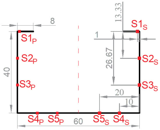
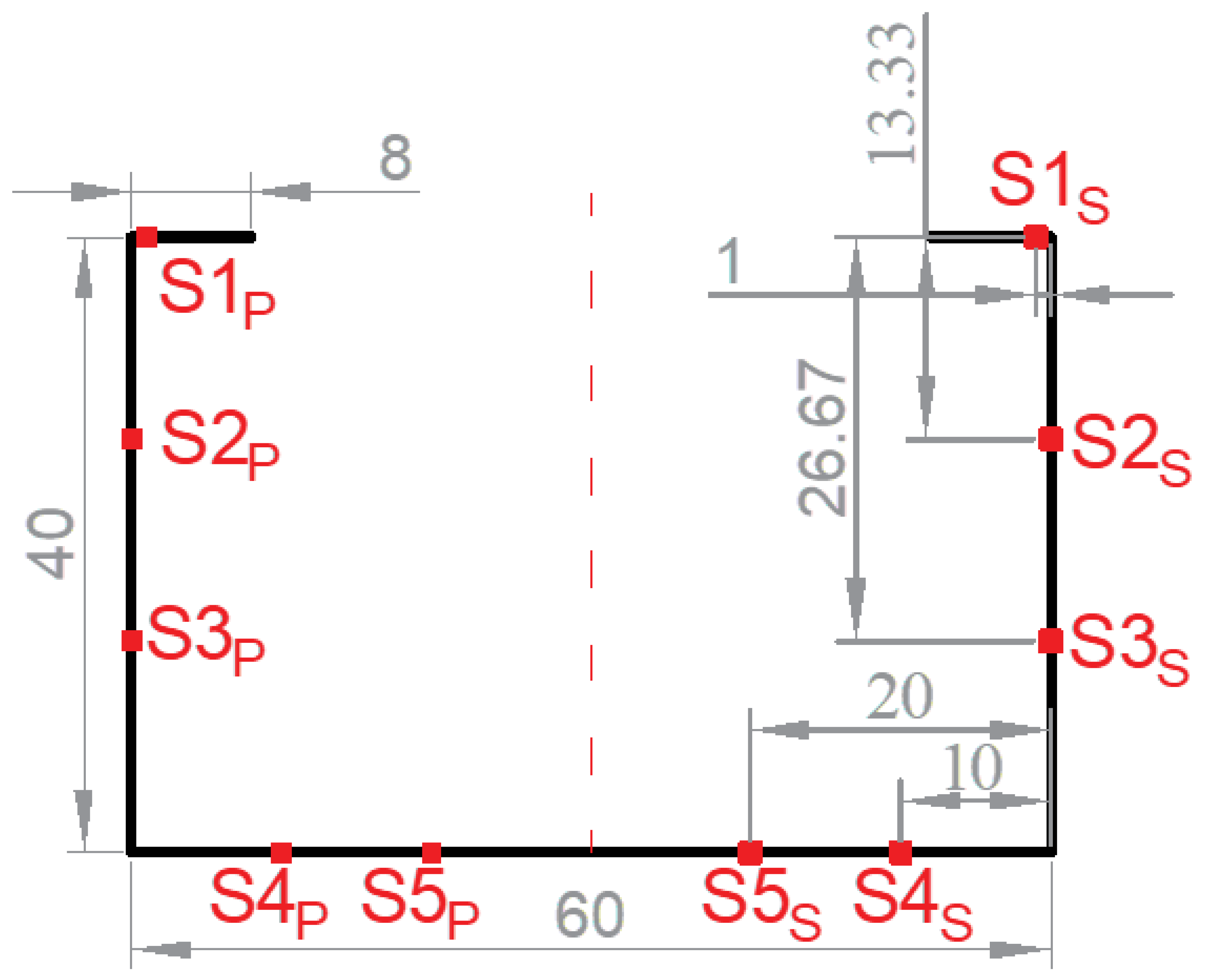
A simplified U-shaped uniform beam is designed to validate the proposed sectional load conversion method. The simplified U-shaped beam’s cross-section is designed to have the same vertical and horizontal moments of inertia as the amidship section of the target containership. The thickness of all the plates is set at 50 mm. The beam length is 400 m, which is the same as the containership’s overall length. Figure 7 depicts the cross-section of the designed U-shaped uniform beam. The corresponding FE model was built in Abaqus. The material properties of high-strength steel are defined for the beam. Five sensors are positioned on each of the port and starboard sides at the measured section to monitor the longitudinal stress, where S1 is on the deck, S2 and S3 are on the side plate, and S4 and S5 are on the bottom plate.

Figure 7. Sketch of the simplified U-shaped beam’s cross-section (unit: m).

To study the accuracy of the developed load estimation method, the estimated load components at the amidship section in Table 2 are applied to the beam systematically, covering both independent and combined loading conditions sequentially, as shown in Table 3.

Table 3. Scheme of applied designed external load conditions on the beam.

Scheme ID	External Load Combination
I	VBM only
II	HBM only
III	VBM and HBM
IV	VBM, HBM and TM
V	Fx, VBM, HBM and TM

It is known that the number and position of the monitoring sensors will affect the accuracy of the estimated load results. Thus, sensor optimization arrangement is systematically studied in this section. A total of 26 possible sensor combination cases are listed in Table 4. Sensors on both sides are adopted for each case.

Table 4. Combinations of the sensors.

Sensor Case	Sensor No.	Sensor Case	Sensor No.
C1	S1, S2	C14	S1, S3, S4
C2	S1, S3	C15	S1, S3, S5
C3	S1, S4	C16	S1, S4, S5
C4	S1, S5	C17	S2, S3, S4
C5	S2, S3	C18	S2, S3, S5
C6	S2, S4	C19	S2, S4, S5
C7	S2, S5	C20	S3, S4, S5
C8	S3, S4	C21	S1, S2, S3, S4
C9	S3, S5	C22	S1, S2, S3, S5
C10	S4, S5	C23	S1, S2, S4, S5
C11	S1, S2, S3	C24	S1, S3, S4, S5
C12	S1, S2, S4	C25	S2, S3, S4, S5
C13	S1, S2, S5	C26	S1, S2, S3, S4, S5

4.2. Validation Under Pure Bending Moment Loading

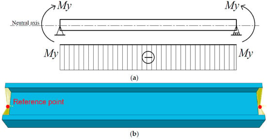
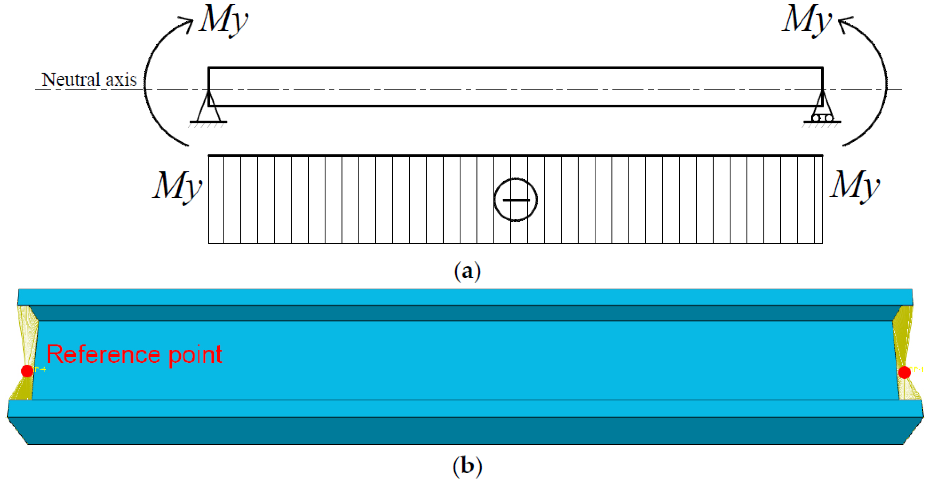
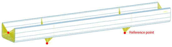
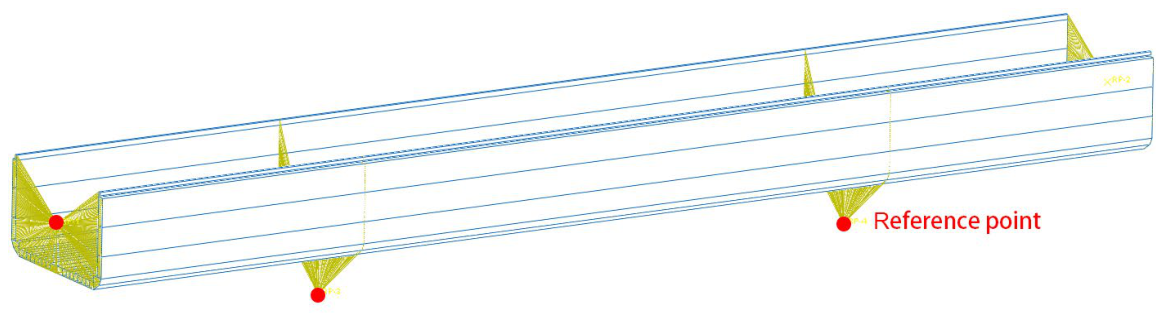
Fundamental validation is carried out using pure vertical or horizontal bending moments and their combinations (Schemes I to III). Taking pure vertical bending of Scheme I as an example, the loads and constraints applied on the beam model in Abaqus are shown in Figure 8. In the x-o-z plane, the left end constrains both planar translational degrees of freedom (DOFs), while the right end only constrains the vertical translational DOF but releases the lateral translational DOF so as to avoid the longitudinal stress due to the beam’s longitudinal deformation. The rotational DOFs at both ends is released. All nodes at the two end sections of the beam are constrained to a reference point located at the neutral axis height using kinematic coupling. External loads and boundary conditions can be applied to the reference points. The six DOFs of these nodes correlate with the conditions acting on the reference points. Static analysis is conducted. The mesh size is set to 0.5 m, and a total of 125,600 FE elements are generated. In order to ensure the accuracy of the local stress, a fine mesh is used in this study. On the other hand, this beam is simple and only static or quasi-static analyses are involved, so the computational efficiency is not an issue of concern. Therefore, a relatively small mesh size is adopted to obtain accurate stress values at specific points of monitoring.

Figure 8. Implementation of pure bending on the beam in Abaqus. (a) Load and boundary conditions of pure vertical bending. (b) Kinematic coupling to the reference points at the two ends.

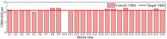
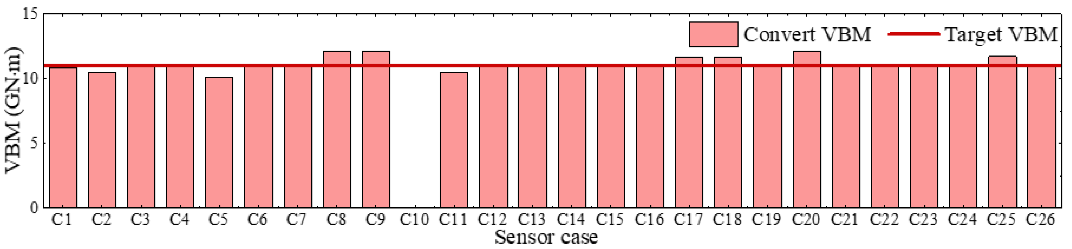
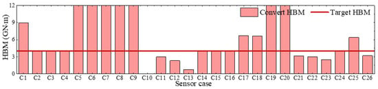
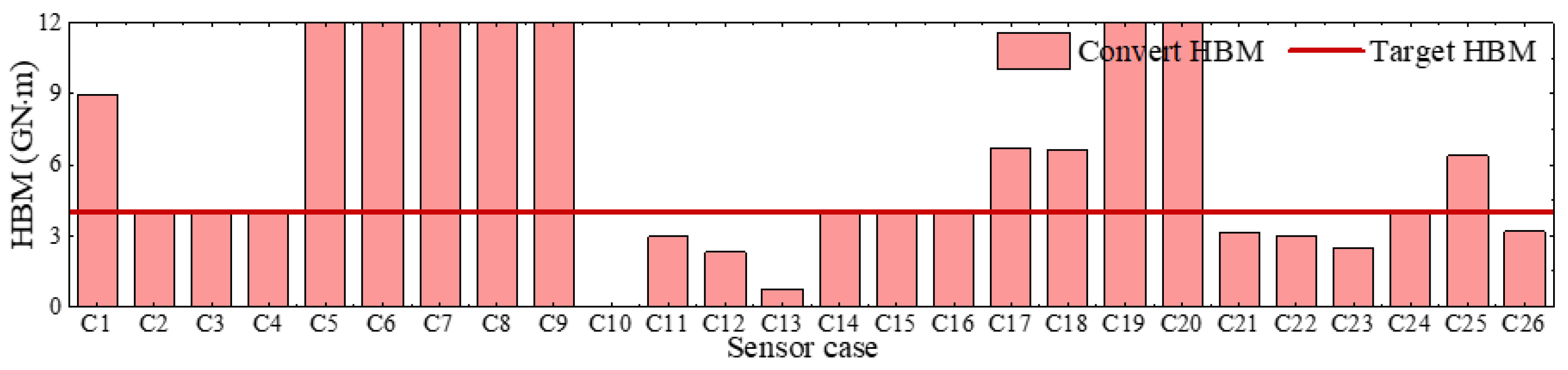
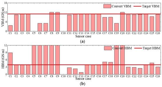
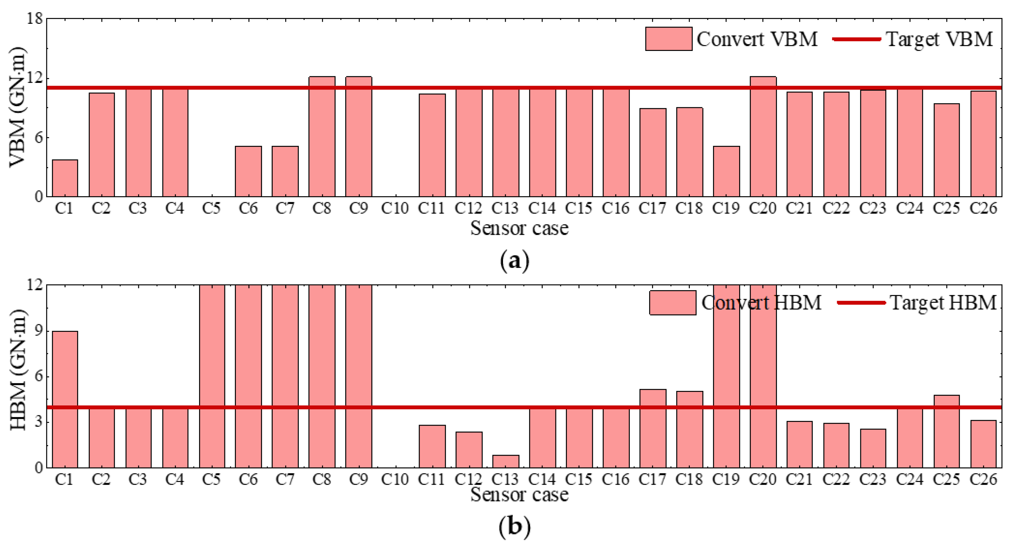
The loading conditions of Schemes I to III are applied to the beam successively. For each loading scheme, all 26 sensor arrangement cases are used to inversely estimate the sectional loads for accuracy comparison and point optimization. The estimated sectional loads by the 26 sensor arrangement cases for the three loading schemes in comparison with the target values are shown in Figure 9, Figure 10 and Figure 11. It is noted that sensor combination C10 cannot be used. It is seen that in the case of pure VBM (Scheme I), the converted VBM generally agrees well with the target value for almost all the cases. However, only a few sensor arrangement cases are feasible for Schemes II and III when HBM is involved, while other cases could result in large deviations from the target values. Specifically, if the monitoring points rely only on the strain sensors on the side and bottom plates, without strain measurements on the deck, this leads to poor accuracy of the conversion results. This is because the side sensors are located near the neutral axis, which results in small z values in Equation (2). Hence, the coefficients corresponding to the VBM component in the conversion matrix of Equation (13) become small, while the relatively large y values render the coefficients for the HBM component large. Such an imbalance causes the matrix to become ill-conditioned upon conversion. Consequently, when the VBM coefficients are too small for the correct load weights to be identified, the converted VBM may be inaccurate, and most of its contribution is erroneously attributed to the HBM. This is evident in Figure 11. Table 5 lists the potential optimized sensor arrangement cases where the converted load deviation is below 1%. To summarize, for the U-shaped beam, sensor points should be distributed on both the deck and bottom plate to obtain accurate converted results.

Figure 9. Comparison of converted VBM for different sensor combinations in Scheme I.

Figure 10. Comparison of converted HBM for different sensor combinations in Scheme II.

Figure 11. Comparison of converted bending moments for different sensor combinations in Scheme III. (a) VBM, M_y. (b) HBM, M_z.

Table 5. Summary of error for optimized sensor combination cases.

Sensor Case	Sensor No.	Error (%)
		Scheme I VBM	Scheme II HBM	Scheme III
				VBM	HBM
C3	S1, S4	0.05	–0.09	0.03	–0.24
C4	S1, S5	0.05	–0.35	0.05	–0.34
C14	S1, S3, S4	0.81	0.07	0.80	–0.10
C15	S1, S3, S5	0.81	0.09	0.81	–0.07
C16	S1, S4, S5	0.05	–0.14	0.04	–0.26
C24	S1, S3, S4, S5	0.10	0.04	0.10	–0.12

4.3. Validation Under Multiple Force Component Loading

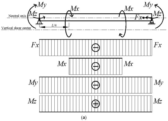
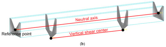
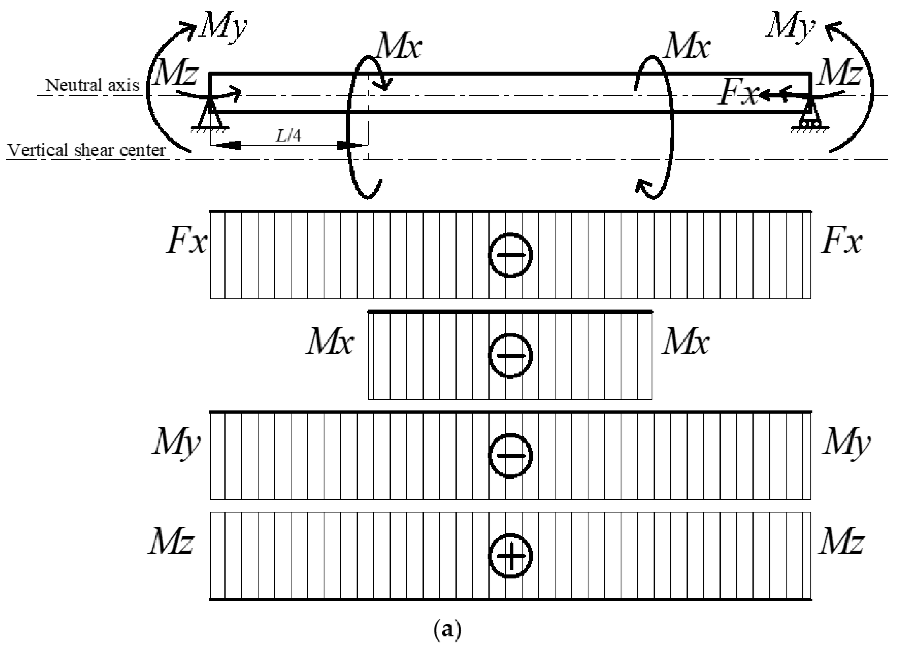
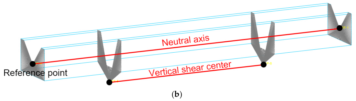
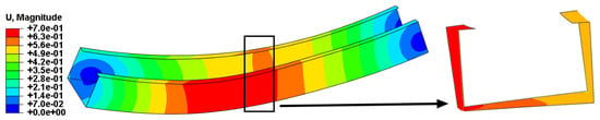
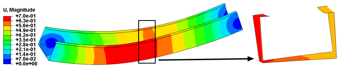
Under the external loads of pure bending, the accuracy of inversely estimated sectional load has been well validated and feasible sensor arrangement cases have been found. In this section, the axial force and torsional moment are applied in addition to bending moments to reproduce more complex force loading conditions. Taking Scheme V as an example, the applied loads and boundary conditions of constraints on the beam structure in Abaqus are shown Figure 12. The boundary condition is the same as that in Section 4.2. The VBM, HBM and axial compressive force are applied to the reference points at the neutral axis height at both ends. Additionally, the torsional moment is applied to the reference points of the shear center at the sections at a distance of L/4 from each end, so as to produce pure torsion without resulting in additional bending moments. It is worth mentioning that the TM applied to a beam with a non-circular cross-section will result in warping involving a bimoment that contributes to the longitudinal strain. The quasi-static analysis is conducted. The deformation of the beam at an amplification factor of 50 under Scheme V is shown in Figure 13.

Figure 12. Implementation of complex loading on the beam in Abaqus. (a) Applied multiple loads and boundary conditions. (b) Kinematic coupling to the reference points.

Figure 13. Nodal displacement contour of the U-shaped beam under complex loading of Scheme V.

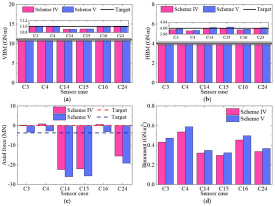
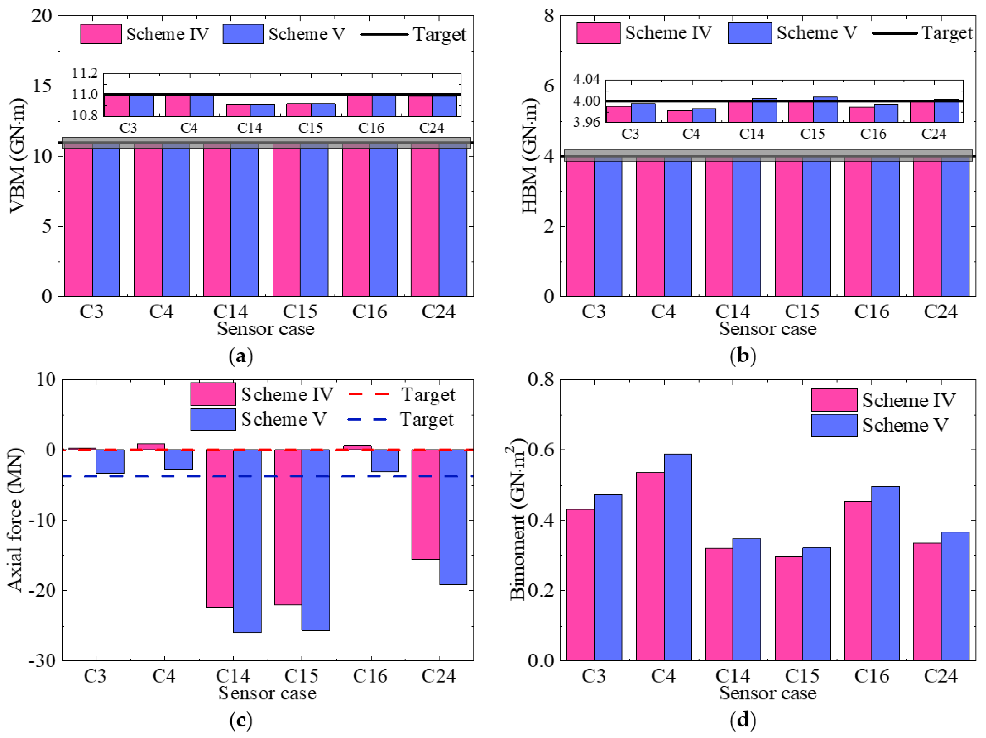
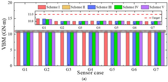
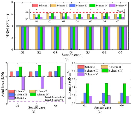
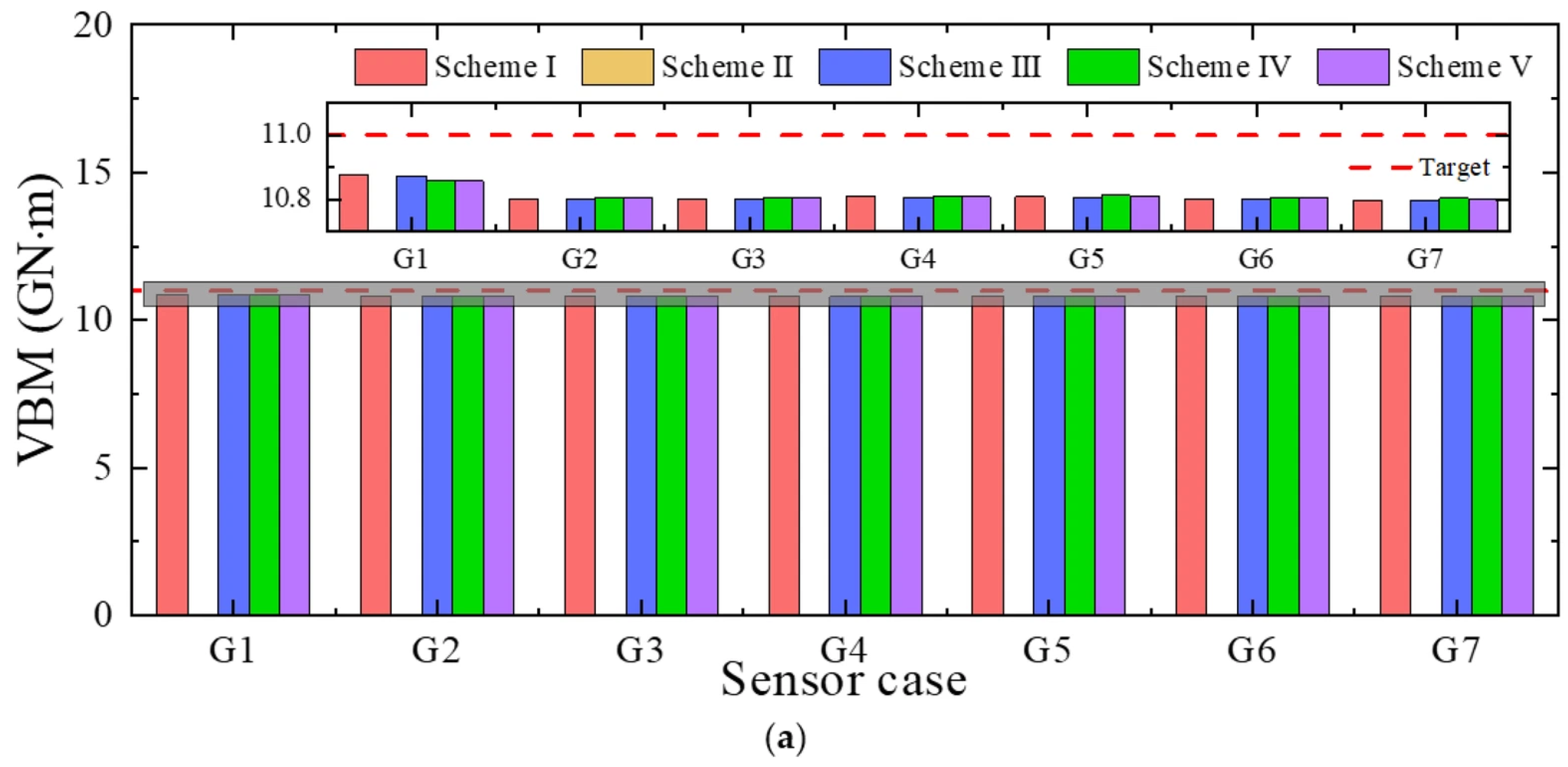
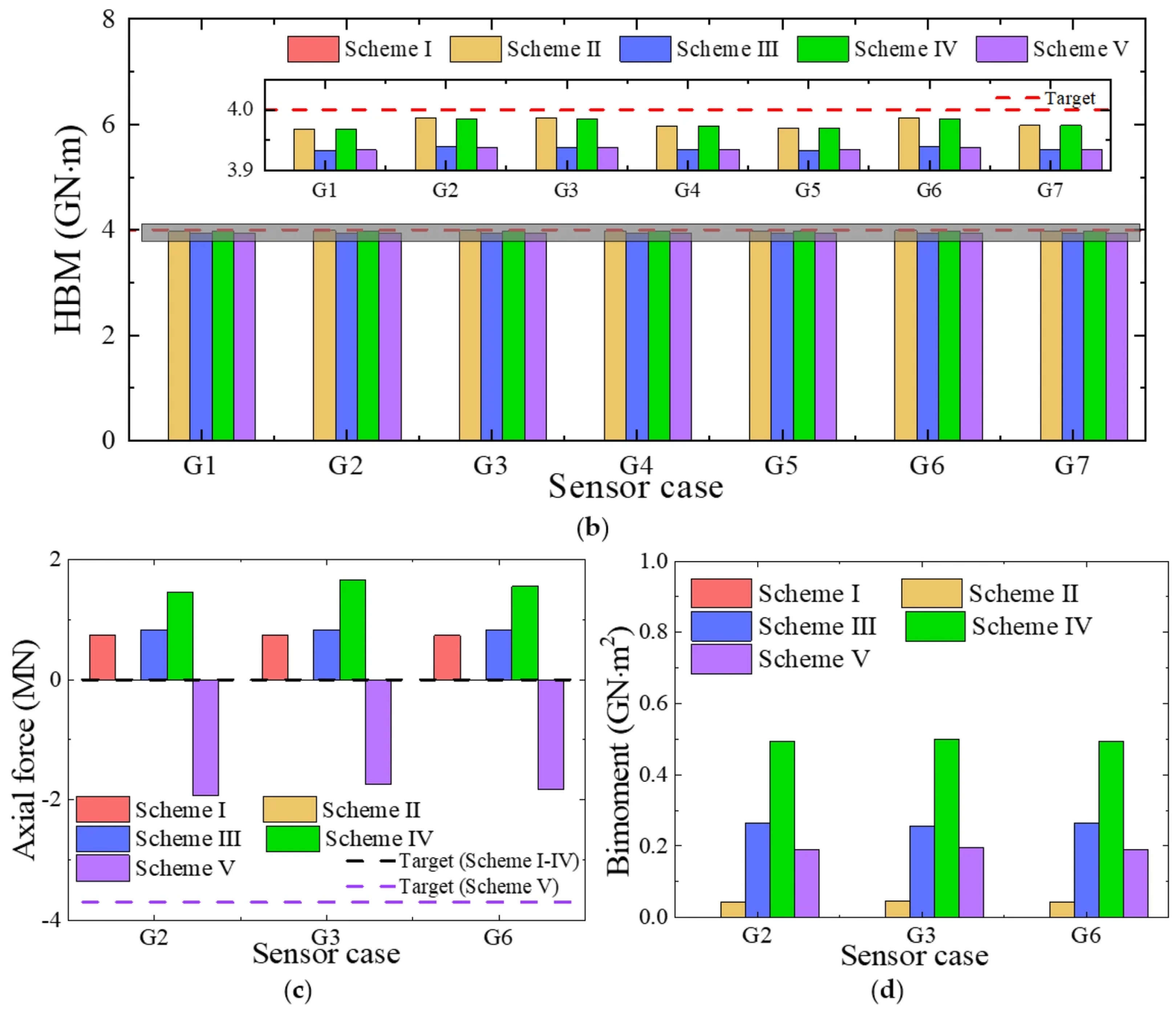
The estimated load conversion results using the optimized sensor arrangement cases listed in Table 5 in comparison with the target values for Schemes IV and V are shown in Figure 14. It is seen that the estimated VBM and HBM have good accuracy even when axial force and torsional moment exist. The maximum differences of VBM and HBM are 0.04% and 0.26%, respectively. However, the axial force and bimoment obtained by different sensor arrangement cases shows obvious difference. The axial force estimated using the three sensor arrangement cases C3, C4 and C16 is close to the target value, while that estimated using the other cases, C14, C15 and C24, differs significantly with the target value. The target value of the bimoment is unknown. The magnitude of the bimoment is small, although there are some differences in the results obtained using the six sensor arrangement cases. This result reveals that accurate load conversion under complex loading conditions relies on longitudinal strain sensors located on the deck and bottom plates, while the sensors on the side plates may even pollute the estimation results.

Figure 14. Comparison of the converted sectional loads when considering torsional moment and axial force. (a) VBM, M_y. (b) HBM, M_z. (c) Axial force, F_x. (d) Bimoment, B.

5. A Uniform Parallel Beam of Containership Amidship Section

In this section, a uniform beam with a simplified amidship section of the 21,000 TEU containership is adopted to conduct the load conversion using both static and dynamic loading conditions for further validation.

5.1. Beam Model Description

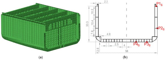
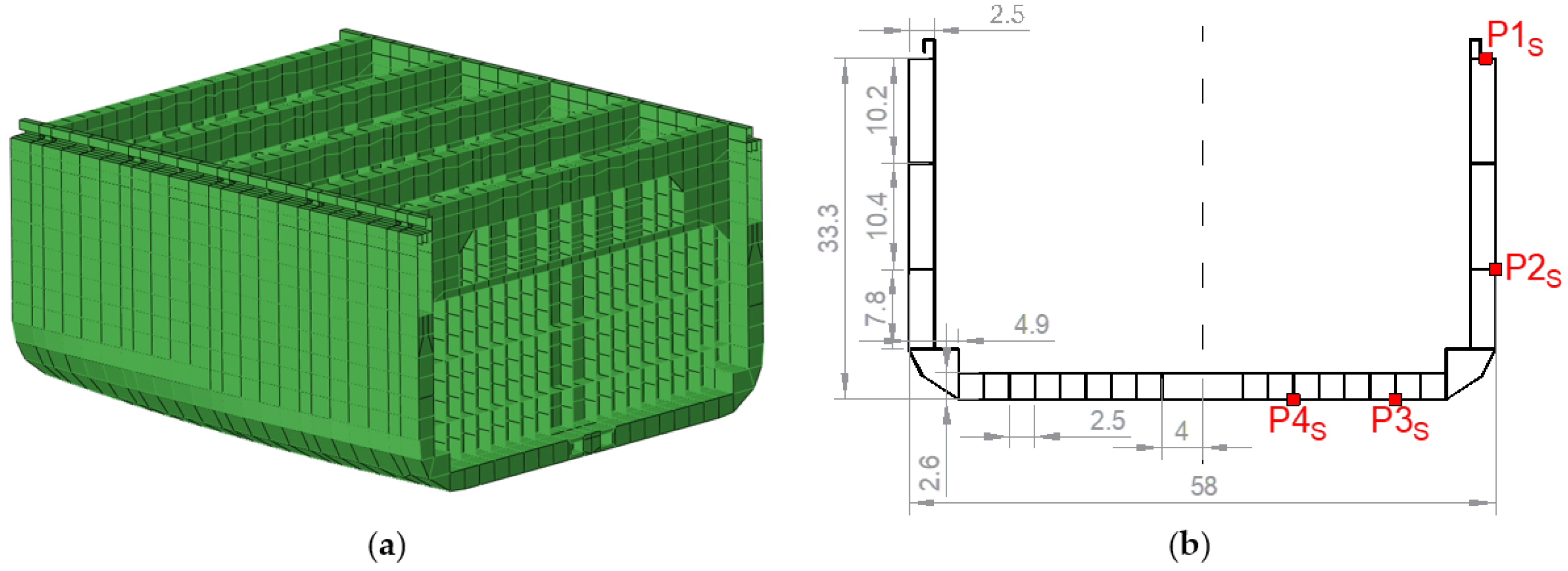
To assess the applicability of the proposed load conversion method to complex hull structures, an extended study is conducted using a uniform beam with a simplified midship section. The beam has a length of 400 m, which is the same as the previous U-shaped beam or the containership. The midship section is simplified from the 21,000 TEU containership. Figure 15 presents the parallel middle segment of the whole-ship finite element (FE) model and the designed cross-section. This cross-section is re-modeled based on the shell element geometry and the positions of its nodes, with all transverse frames ignored for simplification. Material properties of high-strength steel are assigned to the model. A total of eight sensors are symmetrically distributed at each concerned cross-section, with four located on the port side and the other four on the starboard side. The starboard sensor arrangement is shown in Figure 15b, where one is on the deck, one is on the side plate and two are on the bottom plate.

Figure 15. Design of the beam’s cross-section. (a) Parallel body of the ship structure. (b) Sketch of sectional structure and sensor arrangement.

A mesh size of 0.5 m is used to discretize the FE model for the FEA. A total of 69,680 shell elements are generated. The basic parameters such as COG, moment of inertia, shear center and sectorial coordinate that are used in the calculation matrix in Equation (13) are calculated using Dlubal’s software SHAPE-THIN, version 9.18.01 (https://www.dlubal.com/zh). As shown in Table 6, a total of seven sensor arrangement cases are used for the comparative study of load conversion.

Table 6. Designed sensor combinations.

Sensor Case	Sensor No.
G1	P1, P2
G2	P1, P3
G3	P1, P4
G4	P1, P2, P3
G5	P1, P2, P4
G6	P1, P3, P4
G7	P1, P2, P3, P4

5.2. Static Loading Condition

The static FE analysis is conducted. Boundary conditions and external loads are applied in a similar way to those for the U-shaped beam in Section 4.2 (see Figure 12). Figure 16 shows an overview of the beam and its kinematic couplings. All five loading schemes in Table 3 are adopted. Taking Scheme V as an example, the stress distribution and deformation of the beam at an amplification factor of 50 are shown in Figure 17, where local warping can be observed at the middle segment.

Figure 16. Overview of the beam model and kinematic couplings.

Figure 17. Nodal displacement contour of the beam model in Scheme V.

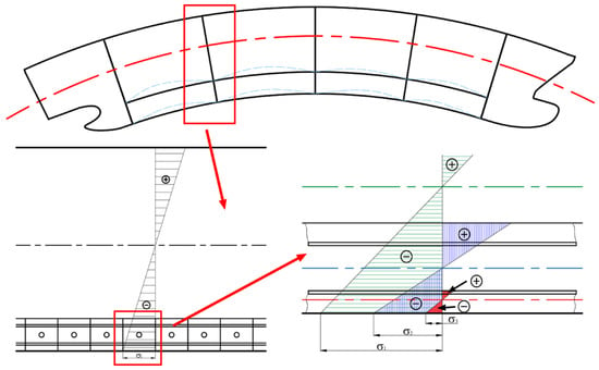
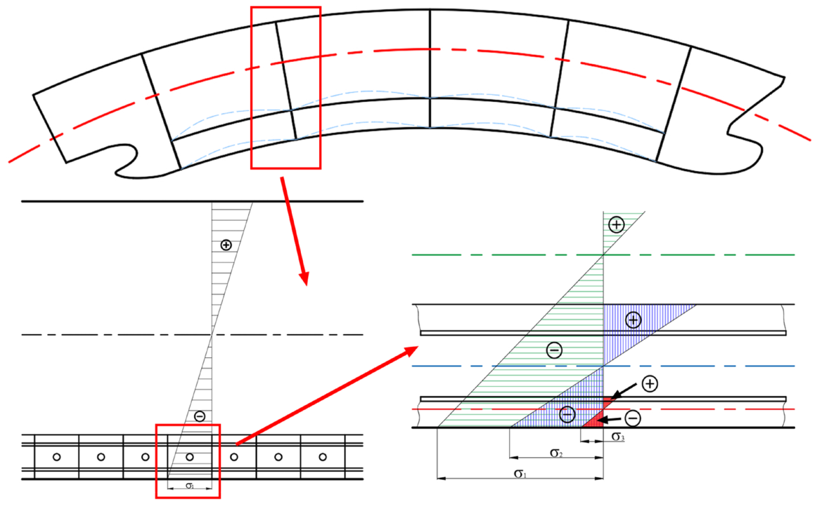
Figure 18 summarizes the converted sectional loads by different sensor combination cases under different external loading schemes. It is noted that since HBM and VBM are not applied in Scheme I and Scheme II, respectively, the corresponding estimated bending moment are close to zero. Generally, the VBM and HBM estimated by all the cases agree well with the target values with errors below 2%, even though the deviation is slightly larger than that of the U-shaped beam in Table 5. This is because the strain measured on the outer bottom plate is a superposition of strain generated by multiple bending components. In the conversion algorithm, the strain caused by the bending of the double bottom plate frame structure is, however, not considered. As shown in Figure 19, in addition to the hull girder overall longitudinal bending, the grillage bending of the double bottom and the plate bending of the outer bottom plate also occur.

Figure 18. Comparison of the converted sectional loads for different external load schemes. (a) VBM, M_y. (b) HBM, M_z. (c) Axial force, F_x. (d) Bimoment, B.

Figure 19. Multiple effects of bending stress on the outer bottom plate.

However, a noticeable deviation is found in the axial force. The reason is that the external VBM produces an axial force component. This is due to a discrepancy between the ideal and the actual neutral axis of vertical bending. Specifically, the theoretical distance from the sensor point to the neutral axis is z_i, while the real value is z_i +∆z. Thus, the real strain is expressed as ${\epsilon }_i={\displaystyle \frac{z_i}{E{I}_y}}{M}_y+{\displaystyle \frac{\Delta z}{E{I}_y}}{M}_z$. The additional term ${\displaystyle \frac{\Delta z}{E{I}_y}}{M}_y$ is regarded as the axial force, which is described as $N=\mathit{EA}\cdot {\displaystyle \frac{\Delta z}{E{I}_y}}{M}_y$. Furthermore, it is observed that the bimoment for the schemes that include an external HBM is non-zero. This is because the shear center of the cross-section is offset from the neutral axis, resulting in warping torsion. Warping torsion gives rise to longitudinal warping normal stresses in the flanges and web.

5.3. Dynamic Loading Condition

A dynamic implicit solver is employed in this section to perform the finite element analysis, which accounts for geometrical nonlinearity. A time-domain solution through direct step-by-step integration of the discretized governing equations can be obtained. At each time step, the solution requires iterative procedures to achieve equilibrium within a specified tolerance. Moderate dissipation, which introduces numerical damping, is adopted to suppress divergence.

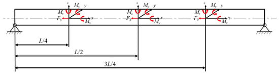
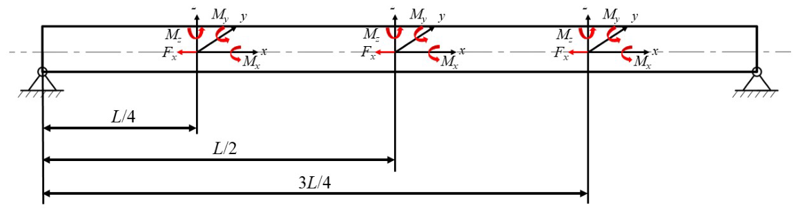
Ships advancing in regular waves are subjected to cyclic loads. Thus, the accurate conversion of periodic loads is crucial for ship load monitoring. As shown in Figure 20, periodic external loads are applied at three typical cross-sections, i.e., L/4, L/2 and 3L/4 from the left end, to represent a complex loading condition. The most complex loading scheme, Scheme V, is used for this study, in which all four kinds of sectional loads are applied. The amplitudes of the sectional loads at different sections are set in accordance with the values specified by the rules in Section 3.2, which are summarized in Table 7. All loads vary periodically at a frequency of ω = 0.6 rad/s, with a phase difference of π/2 between adjacent positions.

Figure 20. Applied loads and boundary conditions of dynamic loading.

Table 7. External loads at different cross-sections.

External Load	3L/4 from the Left End	L/2 from the Left End	L/4 from the Left End
Axial force, Fx (MN)	–3.7sin(0.6t)	–3.7sin(0.6t + π/2)	–3.7sin(0.6t + π)
VBM, My (GN∙m)	7.9sin(0.6t)	11.0sin(0.6t + π/2)	6.9sin(0.6t + π)
HBM, Mz (GN∙m)	2.0sin(0.6t)	4.0sin(0.6t + π/2)	2.0sin(0.6t + π)
TM, Mx (GN∙m)	4.0sin(0.6t)	1.8sin(0.6t + π/2)	4.5sin(0.6t + π)

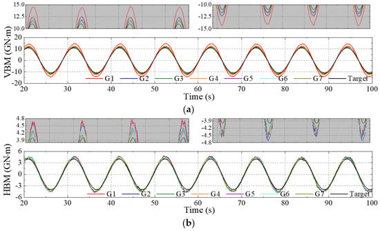
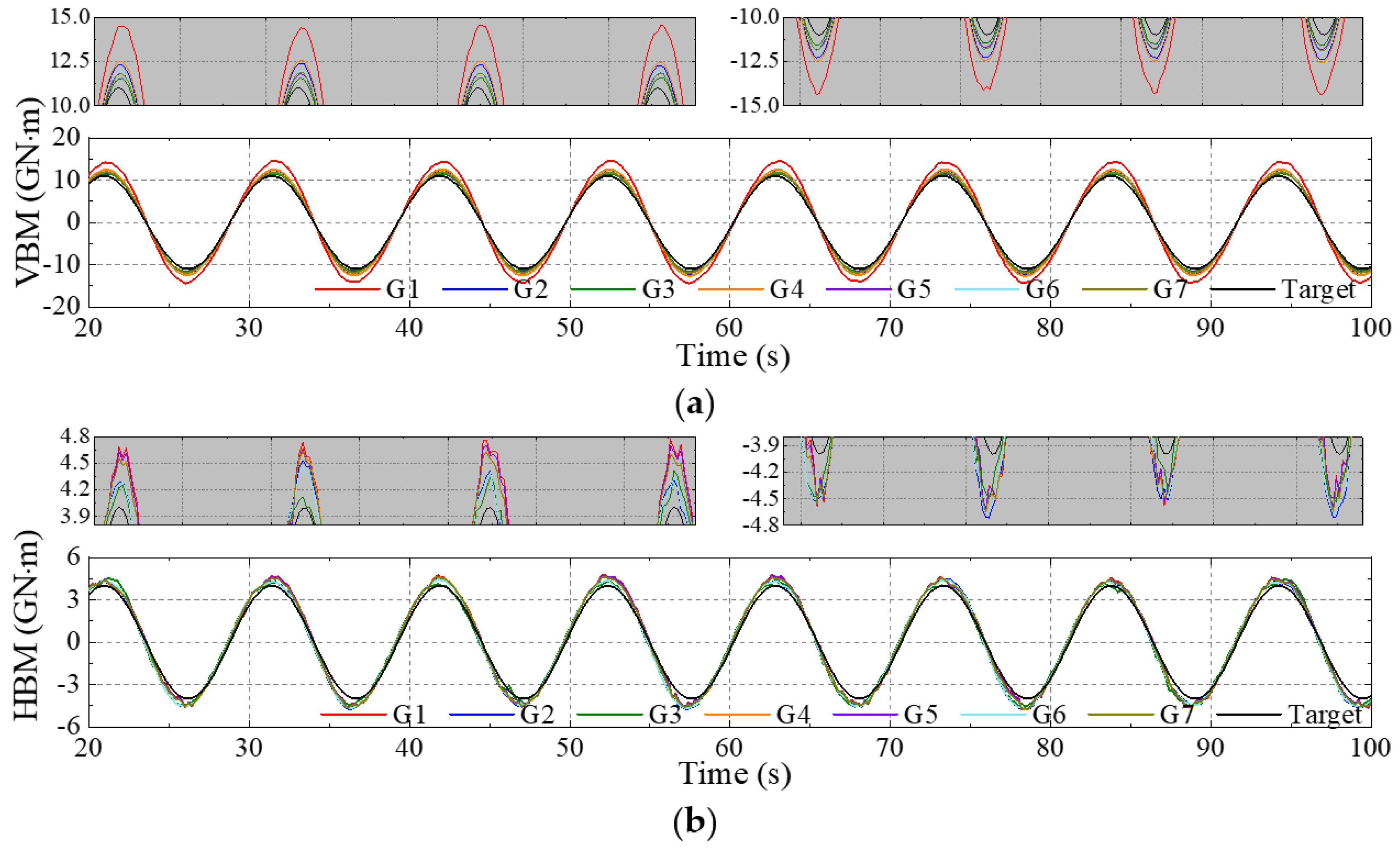
Figure 21 compares the time series of the estimated VBM and HBM loads in the steady regions at the middle section (L/2 from the left end) of the beam by different sensor combinations. Local enlarged views around the crests and troughs are also presented.

Figure 21. Comparison of the converted periodic sectional loads at middle section L/2 by different sensor combinations. (a) Converted VBM. (b) Converted HBM.

To quantify the accuracy of the converted results, error evaluation indices, including mean absolute error (MAE), mean square error (MSE), root mean square error (RMSE) and the coefficient of determination (R²), are used to represent the error between the converted and target time series, which are defined as follows [65]:

$$L_{\mathit{MSE}}={\displaystyle \frac{1}{n}}{\displaystyle \sum _{i=1}^n{\left(y_i^{\mathit{true}}-y_i^{\mathit{pred}}\right)}^2}$$

(25)

$$L_{\mathit{RMSE}}=\sqrt{{\displaystyle \frac{1}{n}}{\displaystyle \sum _{i=1}^n{\left(y_i^{\mathit{true}}-y_i^{\mathit{pred}}\right)}^2}}$$

(26)

$$L_{\mathit{MAE}}={\displaystyle \frac{1}{n}}{\displaystyle \sum _{i=1}^n\left|y_i^{\mathit{true}}-y_i^{\mathit{pred}}\right|}$$

(27)

$$L_{R^2}=1-{\displaystyle \frac{{\displaystyle \sum _{i=1}^n{\left(y_i^{\mathit{true}}-y_i^{\mathit{pred}}\right)}^2}}{{\displaystyle \sum _{i=1}^n{\left(y_i^{\mathit{true}}-\overline{y_i^{\mathit{true}}}\right)}^2}}}$$

(28)

where $y_i^{\mathit{true}}$ is the actual applied external loads, $y_i^{\mathit{pred}}$ is the converted/predicted load, $\overline{y_i^{\mathit{true}}}$ is the average value of the applied external loads, and n is the total number of data samples (5 Hz is used in the present time series).

The results of the evaluation indices for the four optimized combinations (i.e., G1, G3, G5 and G7) are listed in Table 8 and Table 9 for VBM and HBM, respectively. The optimal converted VBM for all the three locations is obtained using sensor combination G3. This suggests that utilizing longitudinal strains measured on the deck edge and the center of the bottom plate enhances conversion accuracy for slender structures. Moreover, optimal HBM conversion is achieved using combinations G5 or G1, which reveals that incorporating longitudinal strain measurements on the side plate can improve the conversion accuracy for HBM. In conclusion, the discussions demonstrate that the case G5 is more effective for comprehensive sectional load conversion. When the load is large, e.g., when the compressive stress exceeds the Euler stress, the stress in the longitudinal members no longer increase proportionally (see Figure 22). The compressive resistance of the flexible members (plates) decreases due to instability, and their stress ceases to increase, while the stress in the adjacent stiffeners (longitudinal girders) increase substantially.

Table 8. Evaluation indices of converted VBM by different sensor combinations.

Location	Sensor Combination	MAE (GN∙m)	MSE (GN2∙m2)	RMSE (GN∙m)	R2
3L/4 from the left end	G1	1.48	2.71	1.65	0.911
	G3	0.29	0.11	0.33	0.997
	G5	0.38	0.19	0.43	0.994
	G7	0.39	0.20	0.45	0.993
L/2 from the left end	G1	2.13	5.69	2.39	0.907
	G3	0.36	0.22	0.47	0.996
	G5	0.52	0.41	0.64	0.993
	G7	0.55	0.42	0.65	0.993
L/4 from the left end	G1	1.45	2.60	1.61	0.889
	G3	0.29	0.11	0.33	0.995
	G5	0.38	0.19	0.43	0.992
	G7	0.39	0.20	0.44	0.992

Table 9. Evaluation indices of converted HBM by different sensor combinations.

Location	Sensor Combination	MAE (GN∙m)	MSE (GN2∙m2)	RMSE (GN∙m)	R2
3L/4 from the left end	G1	0.31	0.13	0.36	0.933
	G3	0.38	0.18	0.42	0.908
	G5	0.31	0.13	0.36	0.933
	G7	0.32	0.14	0.37	0.929
L/2 from the left end	G1	0.34	0.15	0.39	0.981
	G3	0.35	0.17	0.41	0.979
	G5	0.33	0.15	0.38	0.982
	G7	0.34	0.15	0.38	0.982
L/4 from the left end	G1	0.13	0.02	0.15	0.988
	G3	0.35	0.15	0.39	0.924
	G5	0.15	0.03	0.17	0.986
	G7	0.17	0.04	0.19	0.982

Figure 22. Stress distribution on the outer bottom plate due to the instability of the plate.

6. Application to Containership Sailing in Real Sea Waves

The above discussions demonstrate that the proposed load conversion method is feasible for beam models under external concentrated loads. In this section, the method is extended to the cases in which containerships experience external fluid loads when operating in waves, which corresponds as closely as possible to actual ship navigation at sea.

Figure 23 illustrates the scenario of the validation procedure for a containership in waves. The dynamic motion responses and wave loads of the containership in waves were obtained by CFD-FEM simulations [17,53], which consider hydrodynamic force, inertial force and fluid-structure interaction effects. Time series results of ship motions, local stress/strain at any local structural nodes and global sectional loads at any cross-section can be obtained from the high-fidelity numerical simulation. By applying the presented method with the numerically simulated local strain data, the sectional loads can be calculated and then compared with the results directly extracted from the simulations [53].

Figure 23. Flowchart of validation procedure of containership in waves.

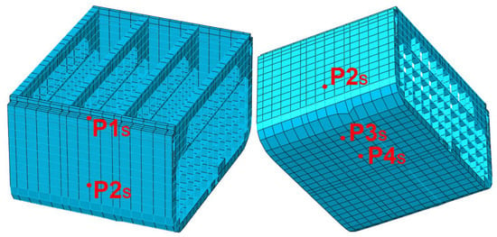
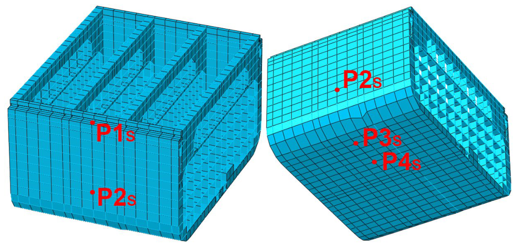
The longitudinal strain or stress at typical positions on the deck, side plate and bottom plate at the amidship cross-section is monitored. Figure 24 presents the strain arrangement on the whole-ship structural model shown from the starboard side as an example.

Figure 24. Point arrangement at the midship.

6.1. Sectional Load Conversion in Regular Head Waves

The results of the containership advancing in regular head waves are used for verification [56]. Table 10 lists the wave parameters and ship condition information. Figure 25 shows a general view of the ship sailing in the regular wave field from the CFD simulation.

Table 10. Wave parameters of regular wave case.

Wave Type	Wave Angle β (°)	Wave Heigh H (m)	Wave Period T (s)	Ship Speed V (kn)
Regular wave	180	12	15.7	18

Figure 25. The containership advancing in regular head waves.

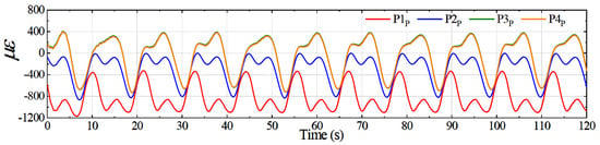
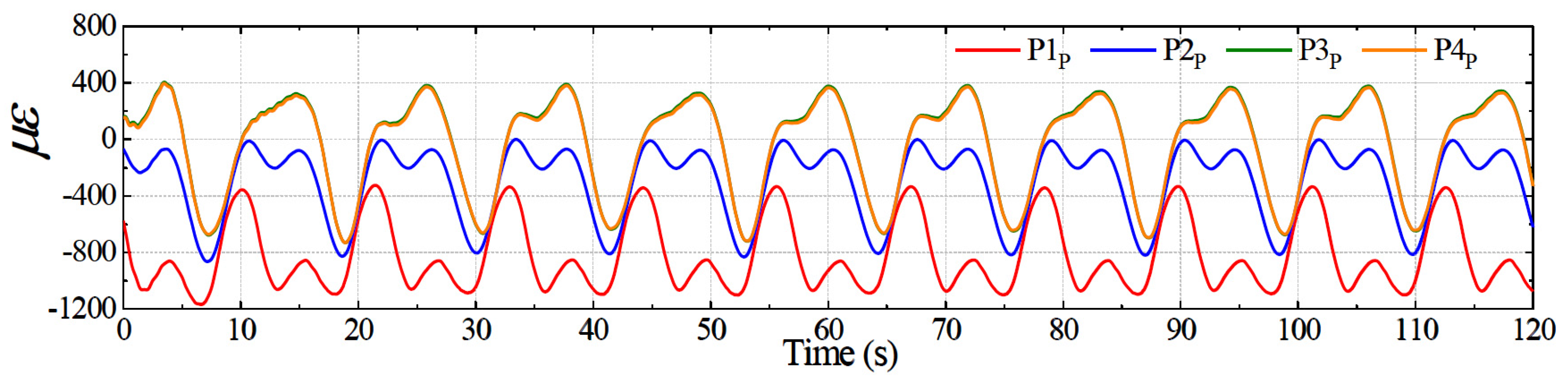
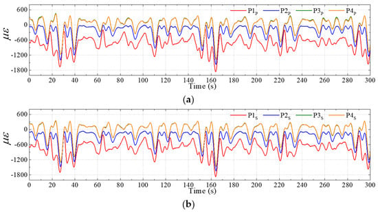
Due to the symmetric response of the ship in head waves, the HBM and TM are theoretically zero. Thus, only VBM and axial force are estimated in this case. Time series of the longitudinal microstrain monitored at different sensors are depicted in Figure 26, which represents the dimension change of the FE panel by its original length. It is seen that the strain exhibits a periodic fluctuation. The curves of P3 and P4 almost coincide, as their distances from the neutral axis are the same.

Figure 26. Time series of the microstrain at different points in a regular wave case.

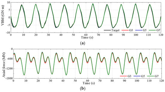
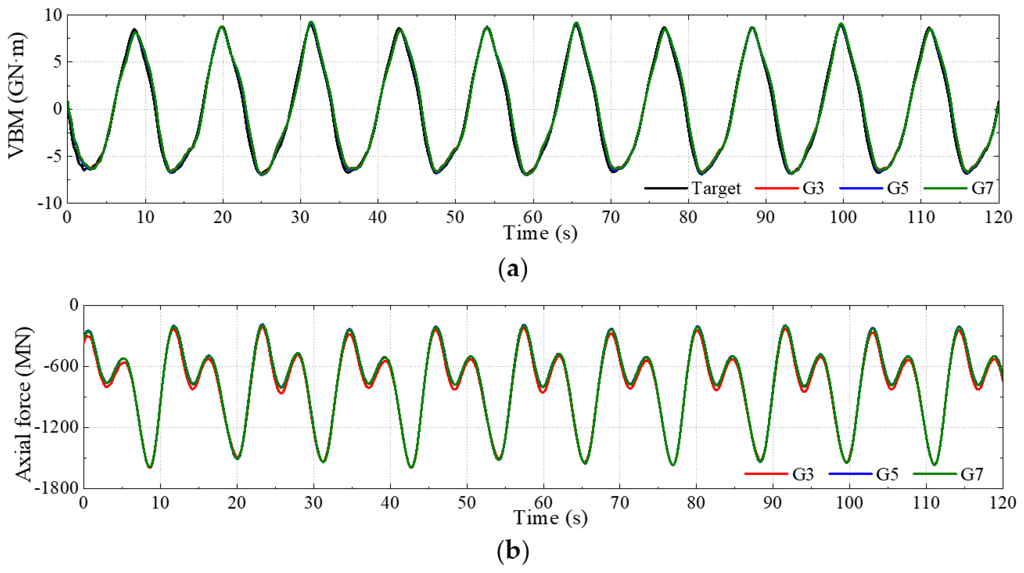
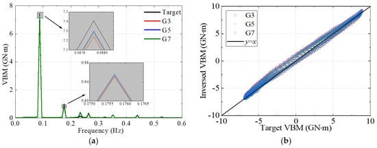
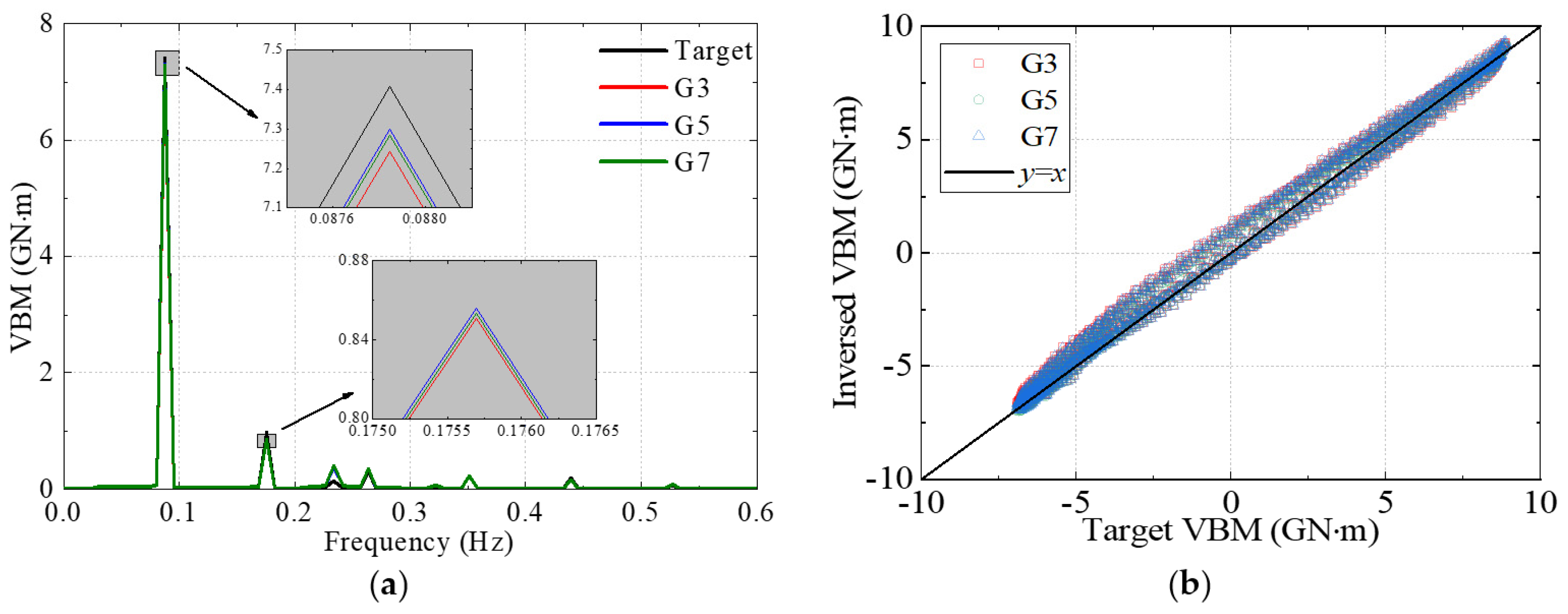
The strain is subsequently used to obtain conversion loads. The comparison of the VBM and axial force converted using different schemes is shown in Figure 27, while Figure 28 shows the comparison of VBM results in the form of frequency spectra and scatter plots. In Figure 28b, a black line (y = x) serves as a reference line, representing the ideal results where the converted values equal the target values. The evaluation indices are also calculated, as depicted in Table 11. Sensor combinations G3, G5 and G7 are adopted to convert VBM, as the above discussion demonstrates their effectiveness. It is evident that the converted load matches the target values for both trends and the low- and high-frequency load components despite small deviations at peaks. The scatter points of VBM are clustered around the reference line. This results from the small difference in the sectional properties between the rebuilt section and the actual one.

Figure 27. Time series of the converted loads by different sensor combinations. (a) VBM. (b) Axial force.

Figure 28. Comparative results of converted VBM in the regular wave case. (a) Frequency spectrum. (b) Scatter diagram.

Table 11. Evaluation indices of VBM in the regular wave case.

Load	Sensor Combination	MAE (GN∙m)	MSE (GN2∙m2)	RMSE (GN∙m)	R2
VBM	G3	0.518	0.369	0.607	0.9868
	G5	0.534	0.381	0.617	0.9864
	G7	0.527	0.377	0.614	0.9866

6.2. Sectional Load Conversion in Short-Crested Irregular Waves

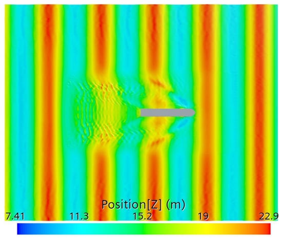
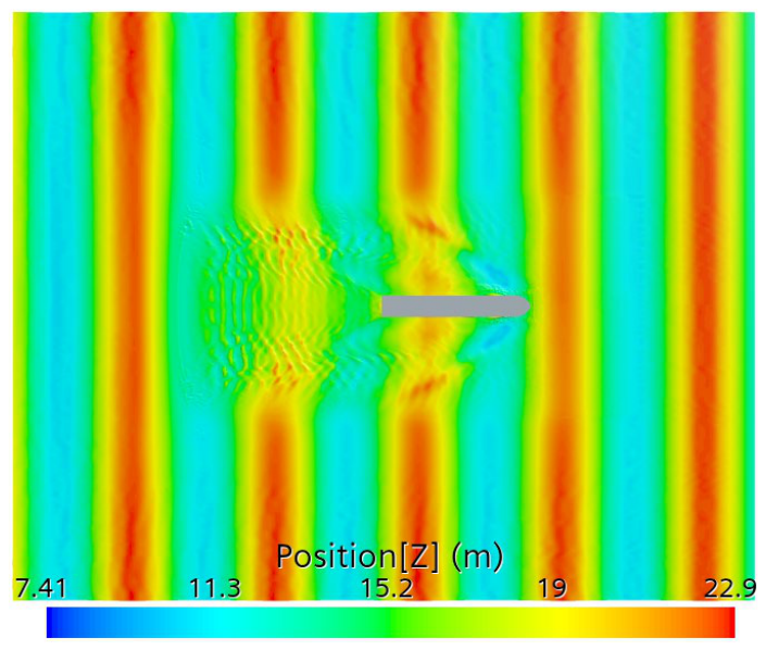
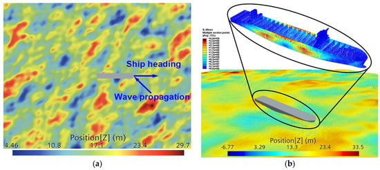
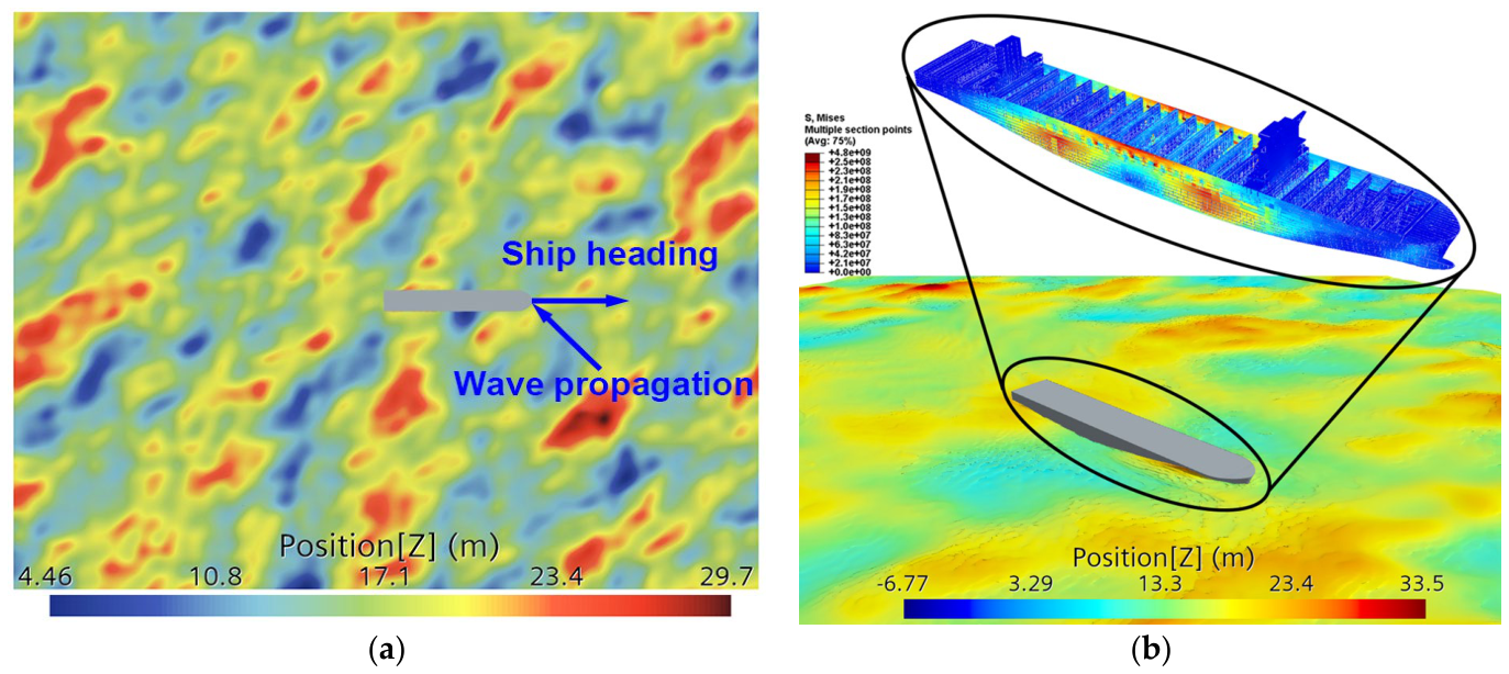
The containership advancing in short-crested irregular waves with the main wave direction set at a bow quarter angle of 135° relative to the ship’s course is studied in this case, with a typical simulation image shown in Figure 29. The wave condition is listed in Table 12.

Figure 29. A containership advances in oblique short-crested waves. (a) General view of the wave field. (b) Local view around the ship.

Table 12. The working case for short-crested irregular waves.

Wave Type	Wave Angle β (°)	Significant Wave Height Hs (m)	Mean Period Tz (s)	Ship Speed V (kn)
Short-crested waves	135	14.5	12.5	22

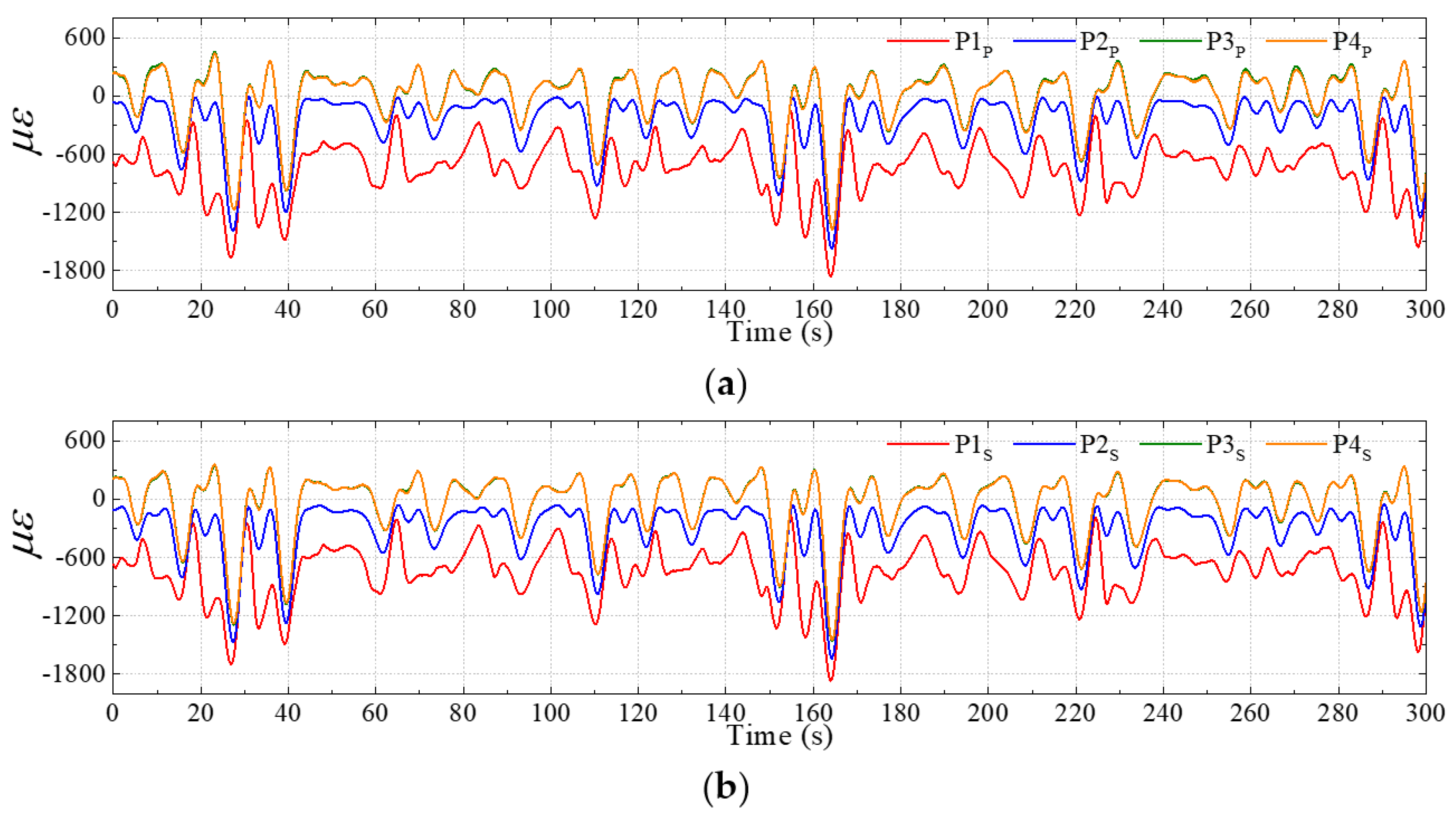
For a ship in short-crested irregular waves, the wave loads on the ship’s hull are asymmetrical. Therefore, the ship is subjected to a combination of axial force, bending moments and a torsional moment. The simulated time series of microstrain at different points in this case, which exhibit high randomness and irregularity, are depicted in Figure 30.

Figure 30. Time series of the microstrain at different points in the short-crested wave case. (a) Port side. (b) Starboard side.

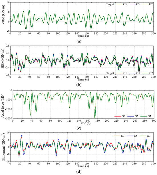
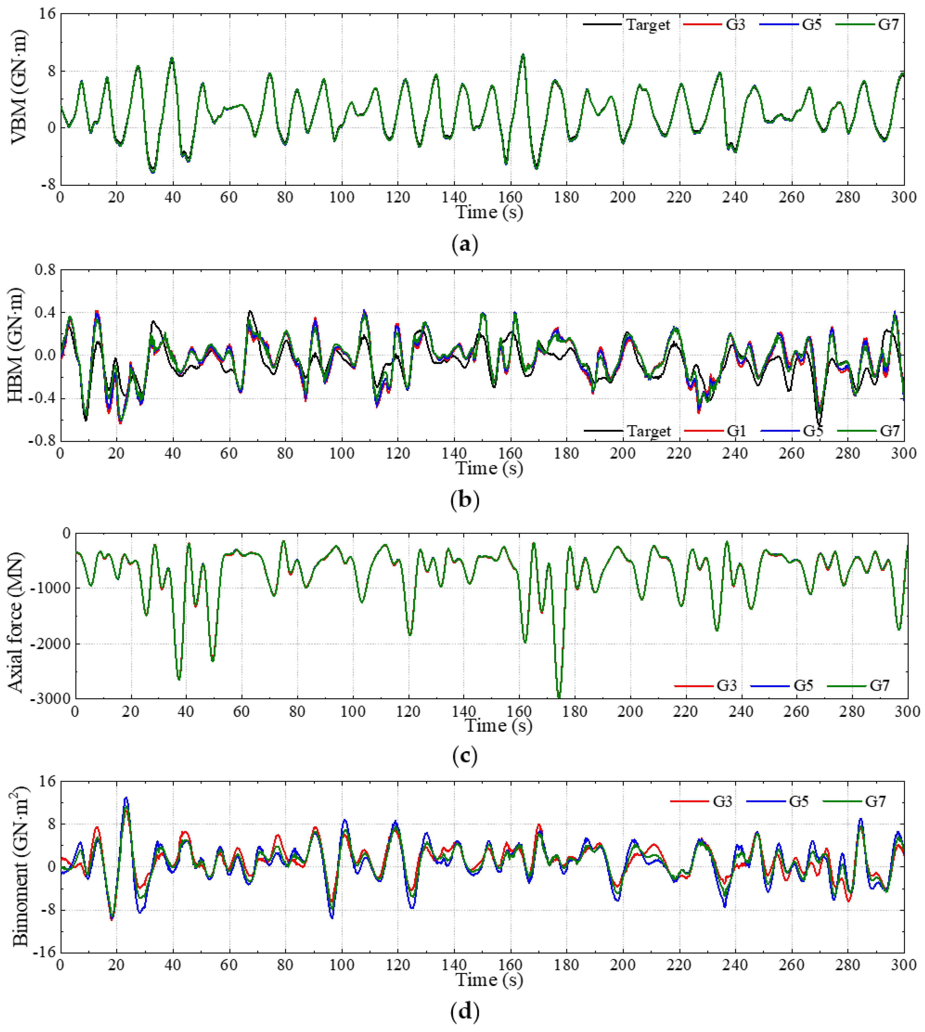
A comparison of the converted time series of the four kinds of sectional loads obtained using different schemes is shown in Figure 31. The optimized sensor combinations for VBM and HBM, respectively, obtained from Table 8 and Table 9, are selected to present the converted results in the figures. Therefore, G3, G5 and G7 are selected for VBM, while G1, G5 and G7 are chosen for HBM. The converted VBM agrees well with the target value, which is consistent with the conclusion from the regular wave case. Although the converted HBM exhibits a similar trend to that of the target value, clear discrepancies are noted in both phase and peak amplitudes. The results are reasonable, as the literature [66] has demonstrated that the symmetric behavior (i.e., VBM) of ships is very close to beam-like behavior. In contrast, discrepancies occur mainly in antisymmetric vibration, where cross-sections are much more prone to deformation and are therefore more likely to violate the beam approximation. According to the experimental data [67] and numerical simulation data [14], the VBM and HBM are of the same order of magnitude for a ship sailing in oblique waves. However, the magnitude of HBM is much lower than VBM in the present results. This is because a horizontal constraint is applied to the FE model to keep the course angle of the ship in oblique waves. Thus, the monitored HBM is not the real value. This study only provides a preliminary validation of the HBM, and more accurate and strict validation of HBM on a ship in waves should be conducted in future work. The converted axial forces among different sensor combinations are close. However, there are slight deviations in the bimoment curves obtained using different schemes.

Figure 31. Comparative time series of the converted loads in the short-crested wave case. (a) VBM. (b) HBM. (c) Axial force. (d) Bimoment.

Table 13 compares the evaluation indices of VBM and HBM, which are calculated using Equations (25)–(28), with the same reference time series used over the same evaluation interval from 0 s to 300 s. It is found that even in short-crested waves, the VBM conversion demonstrates high stability and precision with an R² of 0.98. However, even for the optimal combination G7, the coefficient of determination of HBM is as low as 0.54.

Table 13. Evaluation indices of converted loads in the short-crested wave case.

Load	Sensor Combination	MAE (GN∙m)	MSE (GN2∙m2)	RMSE (GN∙m)	R2
VBM	G5	0.188	0.053	0.230	0.9846
	G7	0.149	0.034	0.184	0.9866
HBM	G5	0.103	0.017	0.130	0.3835
	G7	0.090	0.013	0.112	0.5381

7. Conclusions

This study develops a physics-based strain-driven load conversion method to estimate global sectional loads on real ship hull girders. Static and dynamic numerical validations are performed on simplified beam models and a 21,000 TEU containership under realistic wave environments, and the main conclusions are summarized as follows.

(1) The longitudinal strain measured at local locations on the hull is the superposition of strain components induced by axial force, vertical bending moment, horizontal bending moment and warping bimoment from restrained torsion. Single-point strain cannot accurately evaluate global sectional loads. The derived load conversion matrix enables the determination of multi-component sectional loads from at least four independent longitudinal strain measurements, offering general applicability for slender thin-walled beam-type structures.

(2) Sensor layout significantly governs conversion accuracy. Sensors arranged on deck and bottom plates yield much better performance for vertical bending moment reconstruction. However, sensor points located on side shells may introduce estimation errors in VBM, but they can improve the conversion accuracy for HBM to some extent. Among the tested sensor combinations, schemes adopting deck-edge measuring points together with bottom-plate measuring points achieve superior overall accuracy for VBM conversion under both static and periodic dynamic loads, while the incorporation of measuring points on side shells is helpful for HBM conversion.

(3) For the 21,000 TEU containership under regular head waves, the proposed method reproduces time series of VBM with high fidelity against CFD-FEM reference results, with a coefficient of determination R² exceeding 0.98. Under oblique short-crested irregular waves, VBM conversion maintains satisfactory precision, while HBM conversion suffers obvious phase and amplitude deviations, which are partly attributed to artificial horizontal constraints applied in the global finite element model.

This analytical load conversion approach avoids heavy dependence on massive training datasets required by data-driven methods and possesses clear physical interpretability. It can support real-time sectional load reconstruction for ship-board structural health monitoring systems. Further work should focus on improving HBM and bimoment conversion accuracy and further enhancing the method’s applicability for comprehensive six-degree-of-freedom global load monitoring on real ships.

References

- Jiao, J.; Chen, Z.; Xu, W.; Jiang, C.; Chen, S. CFD-FEM simulation of ship motions and loads in oblique regular waves. Chin. J. Ship Res. 2025, 20, 88–98. (In Chinese) [Google Scholar] [CrossRef] [Scilit]
- Jiao, J.; Chen, Z.; Chen, S.; Jiang, C.; Si, H. Ship hydroelastic responses in wind waves and swell combined realistic seas by numerical simulation and large-scale model sea trial. Ocean Eng. 2026, 348, 124100. [Google Scholar] [CrossRef] [Scilit]
- Yang, X.; Shi, H.; Chai, W.; Lv, C.; Feng, P.; Wu, D. Study on ice load characteristics of polar ships during oblique sailing based on discrete element method. Chin. J. Ship Res. 2026, 21, 349–357. (In Chinese) [Google Scholar]
- Okasha, N.M.; Frangopol, D.M.; Decò, A. Integration of structural health monitoring in life-cycle performance assessment of ship structures under uncertainty. Mar. Struct. 2010, 23, 303–321. [Google Scholar] [CrossRef] [Scilit]
- Sadeghian, M. The reliability assessment of a ship structure under corrosion and fatigue, using structural health monitoring. Int. J. Eng. 2022, 35, 1765–1778. [Google Scholar] [CrossRef] [Scilit]
- Yang, Z.; Guo, L.; Yuan, Y.; Tang, W. Review and prospects of key technologies for large language model-driven ship structural health monitoring systems. Chin. J. Ship Res. 2025, 20, 3–18. (In Chinese) [Google Scholar]
- CCS. Rules for Classification of Sea-Going Steel Ships. 2024. Available online: https://www.ccs.org.cn/ccswzen/articleDetail?id=202406120219943379 (accessed on 12 June 2024).
- Zhu, S.; Moan, T. New insight into the wave-induced nonlinear vertical load effects of ultra-large container ships based on experiments. J. Mar. Sci. Technol. 2013, 18, 87–114. [Google Scholar] [CrossRef] [Scilit]
- Vijith, P.P.; Rajendran, S. Hydroelastic effects on the vertical bending moment of a container ship in head and oblique seas. Ocean Eng. 2023, 285, 115385. [Google Scholar] [CrossRef] [Scilit]
- Wei, Y.; Incecik, A.; Tezdogan, T. A fully coupled CFD-DMB approach on the ship hydroelasticity of a containership in extreme wave conditions. J. Mar. Sci. Eng. 2022, 10, 1778. [Google Scholar] [CrossRef] [Scilit]
- Chen, Z.; Jiao, J.; Xu, W.; Jiang, C.; Chen, S. Numerical simulation of ship hydroelastic responses in short-crested irregular waves. Mar. Struct. 2025, 103, 103858. [Google Scholar] [CrossRef] [Scilit]
- Jiao, J.; Ren, H.; Adenya, C.A. Experimental and numerical analysis of hull girder vibrations and bow impact of a large ship sailing in waves. Shock Vib. 2015, 1, 706163. [Google Scholar] [CrossRef] [Scilit]
- Bouscasse, B.; Merrien, A.; Horel, B.; De Hauteclocque, G. Experimental analysis of wave-induced vertical bending moment in steep regular waves. J. Fluids Struct. 2022, 111, 103547. [Google Scholar] [CrossRef] [Scilit]
- Chen, Z.; Jiao, J.; Chang, X.; Ma, B. Numerical and experimental study of asymmetrical wave loads and hydroelastic responses of ship in oblique regular waves. Appl. Ocean Res. 2024, 153, 104254. [Google Scholar] [CrossRef] [Scilit]
- Vijith, P.P.; Rajendran, S.; Wang, S.; Guedes Soares, C. Numerical assessment of wave-induced motions and rigid bending and torsional loads acting on large slender ships in various operating conditions using a 2D time domain method. Ocean Eng. 2025, 335, 121524. [Google Scholar] [CrossRef] [Scilit]
- Zhang, W.; Wang, J.; Guo, H.; Liu, Y.; Wan, D. Numerical investigations of ship hydroelasticity of a 20,000 TEU containership based on CFD-MBD method. Ocean Eng. 2025, 317, 120061. [Google Scholar] [CrossRef] [Scilit]
- Chen, Z.; Jiao, J.; Yang, Y.; Xie, H.; Wang, S.; Guedes Soares, C. High-fidelity numerical tank for ship seakeeping and wave loads of full-scale whole-ship structures in short-crested sea waves. Mar. Struct. 2026; submitted.
- Chen, Z.; Zhao, N.; Zhao, H.; Guo, R.; Zhao, W. Experimental parametric study on hydroelastic behaviour of a 15000-TEU container ship based on segmented ship model. Ships Offshore Struct. 2023, 18, 948–959. [Google Scholar] [CrossRef] [Scilit]
- Jiao, J.; Ren, H.; Sun, S.; Adenya, C.A. Experimental investigation of wave-induced ship hydroelastic vibrations by large-scale model measurement in coastal waves. Shock Vib. 2016, 1, 9296783. [Google Scholar] [CrossRef] [Scilit]
- Jiao, J.; Sun, S.; Ren, H. Predictions of wave induced ship motions and loads by large-scale model measurement at sea and numerical analysis. Brodogradnja 2016, 67, 81–100. [Google Scholar] [CrossRef] [Scilit]
- Jiao, J.; Ren, H.; Adenya, C.A.; Chen, C. Development of a shipboard remote control and telemetry experimental system for large-scale model’s motions and loads measurement in realistic sea waves. Sensors 2017, 17, 2485. [Google Scholar] [CrossRef] [Scilit] [PubMed]
- Jiao, J.; Ren, H.; Chen, C. Model testing for ship hydroelasticity: A review and future trends. J. Shanghai Jiaotong Univ. (Science) 2017, 22, 641–650. [Google Scholar] [CrossRef] [Scilit]
- Grammatikopoulos, A. A review of physical flexible ship models used for hydroelastic experiments. Mar. Struct. 2023, 90, 103436. [Google Scholar] [CrossRef] [Scilit]
- Grammatikopoulos, A.; Banks, J.; Temarel, P. The design and commissioning of a fully elastic model of a uniform container ship. Mar. Struct. 2021, 78, 103014. [Google Scholar] [CrossRef] [Scilit]
- Chen, Y.; Zhang, S.; Chen, W.K.; Magee, A. Design, construction and testing of a fully elastic ship model for investigating hydro-elastic responses of container ships. Mar. Struct. 2024, 98, 103663. [Google Scholar] [CrossRef] [Scilit]
- Grammatikopoulos, A.; Banks, J.; Temarel, P. Prediction of the vibratory properties of ship models with realistic structural configurations produced using additive manufacturing. Mar. Struct. 2020, 73, 102801. [Google Scholar] [CrossRef] [Scilit]
- Kamour, A.M.; Hjaji, M.A.; Nagiar, H.M. Super convergent finite beam element for torsional vibration of open thin-walled vlasov beam under torsional excitations. Afr. J. Adv. Pure Appl. Sci. 2025, 4, 100–117. [Google Scholar]
- Zhou, B.; Amini-Afshar, M.; Bingham, H.B.; Shao, Y.; Henshaw, W.D. Solving for hydroelastic ship response using Timoshenko beam modes at forward speed. Ocean Eng. 2024, 300, 117267. [Google Scholar] [CrossRef] [Scilit]
- Prini, F.; Benson, S.; Birmingham, R.W.; Dow, R.S.; Ferguson, L.J.; Sheppard, P.J.; Phillips, H.J.; Johnson, M.C.; Mediavilla Varas, J.; Hirdaris, S. Full-scale seakeeping trials of an all-weather lifeboat. In Proceedings of the SURV 9 Conference, Surveillance, Pilot & Rescue Craft, London, UK, 18 April 2018; The Royal Institution of Naval Architects: London, UK, 2018; pp. 25–36. [Google Scholar]
- Tomczak, M.T.; Wojcikowski, M.; Pankiewicz, B.; Łubiński, J.; Majchrowicz, J.; Majchrowicz, D.; Walasiewicz, A.; Kilinski, T.; Szczerska, M. Stress monitoring system for individuals with autism spectrum disorders. IEEE Access 2020, 8, 228236–228244. [Google Scholar] [CrossRef] [Scilit]
- Alarcón, M.; Soto, P.; Hernández, F.; Guindos, P. Structural health monitoring of South America’s first 6-Story experimental light-frame timber-building by using a low-cost RaspberryShake seismic instrumentation. Eng. Struct. 2023, 275, 115278. [Google Scholar] [CrossRef] [Scilit]
- Shen, R.; Hou, Z.; Yuan, Z.; Li, Y.; Gu, Y. Development of a Three-dimensional Stress Monitoring System for Coal Rock and its Application in a Mine. Rock Mech. Rock Eng. 2024, 57, 1983–1996. [Google Scholar] [CrossRef] [Scilit]
- Hu, Z.; Elchalakani, M.; Hassanli, R.; Ran, H.; Sadakkathulla, M.A.; Nie, S. Structural health monitoring of lightweight concrete beams strengthened with ultra-lightweight ECC-FRP mesh composite. Eng. Struct. 2025, 322, 119224. [Google Scholar] [CrossRef] [Scilit]
- Silionis, N.E.; Anyfantis, K.N. Optimal sensor placement for corrosion induced thickness loss monitoring in ship structures. Mar. Struct. 2024, 93, 103524. [Google Scholar] [CrossRef] [Scilit]
- Komoriyama, Y.; Ota, D.; Ma, C.; Sawada, H.; Oka, M.; Matsui, S.; Houtani, H. Hull structural strength evaluation based on fiber bragg gratings pressure sensors to measure spatial pressure distribution on ship’s hull in waves. In Proceedings of the International Conference on Offshore Mechanics and Arctic Engineering, Online, 3–7 August 2020; Volume 18434, p. V02AT02A023. [Google Scholar]
- Zheng, Q.; Wang, X.; Zhao, X.; Yang, H.; Xu, C.; Jiang, Z. Research on strain sensor technology applied in structural safety monitoring of ships and offshore engineering. Equip. Environ. Eng. 2023, 20, 83–89. (In Chinese) [Google Scholar]
- Uhl, T. The inverse identification problem and its technical application. Arch. Appl. Mech. 2007, 77, 325–337. [Google Scholar] [CrossRef] [Scilit]
- Wang, F.; Zheng, K.; Chen, B.; Peng, Y.; Liu, K.; Tang, D. Time-domain inversion method of impact loads based on strain monitoring data. Metals 2022, 12, 1279. [Google Scholar] [CrossRef] [Scilit]
- Zheng, Y.; Wu, S.; Li, Y.; Fei, Q. Identify the spatially-correlated random fluctuating pressure on structure from strain data. Aerosp. Sci. Technol. 2021, 119, 107182. [Google Scholar] [CrossRef] [Scilit]
- Guo, H.Z.; Yuen, K.V.; Mu, H.Q. Real-time Bayesian axle load estimation and structural identification of railway bridges under train loads based on strain monitoring. Eng. Struct. 2025, 322, 119195. [Google Scholar] [CrossRef] [Scilit]
- Sha, J.; Leng, J.; Feng, H.; Pei, J.; Wang, Y.; Song, Y. Load Inversion Method for Jacket Platform Structures Based on Strain Measurement Data. J. Mar. Sci. Eng. 2025, 13, 1785. [Google Scholar] [CrossRef] [Scilit]
- Karvelis, P.; Georgoulas, G.; Kappatos, V.; Stylios, C. Deep machine learning for structural health monitoring on ship hulls using acoustic emission method. Ships Offshore Struct. 2021, 16, 440–448. [Google Scholar] [CrossRef] [Scilit]
- Zhou, C.; Chen, L.; Liu, W.; Yin, Q.; Zhang, J. Research on the Inversion Method of Ice Loads on Ships in Broken Ice Channels Using Deep Neural Networks. Results Eng. 2025, 27, 107017. [Google Scholar] [CrossRef] [Scilit]
- Liu, Z.; Wang, Z.; Chu, G.; Yao, X. Structural deformation prediction of underwater exploded ship hull girder using machine learning. J. Mar. Sci. Appl. 2025, 24, 1279–1290. [Google Scholar] [CrossRef] [Scilit]
- Zhang, S.; Zhang, Q.; Li, Z. Real-time wind response prediction and load inversion for skyscraper using deep learning. Eng. Struct. 2025, 343, 121241. [Google Scholar] [CrossRef] [Scilit]
- Jia, Z.; Jia, S.; Su, X.; Fan, Z.; Dai, S.; Sun, F.; Wang, Y. Time-domain inversion of random dynamic loads on offshore platforms based on optimized ensemble learning. Ocean Eng. 2025, 315, 119822. [Google Scholar] [CrossRef] [Scilit]
- Wan, W.; Wu, D.; Liu, H.; Wang, J.; Chen, J. Real-time identification of structural random dynamic loads using strain-based LSTM for Digital Twin applications. Eng. Struct. 2026, 346, 121615. [Google Scholar] [CrossRef] [Scilit]
- Wang, J.; Ying, Y.; Huang, M.; Li, H.; Zhang, M. High-precision identification method for distributed ice loads exerted on hull structures using an enhanced model. J. Mar. Sci. Appl. 2026. [Google Scholar] [CrossRef] [Scilit]
- Zhang, Y.; Wei, S.; Pang, B.; Cheng, H.; Guo, J. Double Damage Identification of Fully Free Beams Based on Curvature Modes. J. Mar. Sci. Appl. 2025, 25, 1238–1251. [Google Scholar] [CrossRef] [Scilit]
- Dui, H.; Liu, D.; Zhang, Z.; Pan, S.; Yang, L. Distributed load recovery approach based on strain measurements. Acta Aeronaut. Astronaut. Sin. 2021, 42, 295–302. (In Chinese) [Google Scholar]
- Guo, A.; Wu, S.; Zheng, Y. Identify aerodynamic pressure load on a 3D wing structure from strain data using surface flattening and subregion interpolation. Aerosp. Sci. Technol. 2024, 151, 109239. [Google Scholar] [CrossRef] [Scilit]
- Zareei, A.; Zhou, X.; Ringsberg, J.W.; Feng, G. An analytical load identification based on the balancing principle for the ship stiffened panels subjected to grounding impact. Eng. Struct. 2025, 341, 120845. [Google Scholar] [CrossRef] [Scilit]
- Chen, Z.; Jiao, J.; Zou, Y. High-fidelity numerical tank for simulation of hydroelastic responses of whole-ship structures in 3D sea waves. J. Mar. Sci. Appl. 2026; accepted. [CrossRef] [Scilit]
- Chen, Z.; Jiao, J.; Xie, H.; Yang, Y. High-fidelity numerical tank for full-scale ship’s fluid-structure interactions in realistic ocean waves. In Proceedings of the International Ocean Offshore and Arctic Engineering Conference, Tokyo, Japan, 7–12 June 2026; p. 174231. [Google Scholar]
- Chen, Z.; Jiao, J.; Xie, H.; Yang, Y. Full-scale CFD-FEM simulation of a whole ship structure accounting for hydroelasticity. In Innovations in Maritime Technology and Engineering; Soares, C.G., Salvado, F.C., Eds.; CRC Press: London, UK, 2026; Volume 1, pp. 339–347. [Google Scholar]
- Jiao, J.; Chen, Z.; Xie, H.; Yang, Y. Full-scale simulation of containership motion and load responses by whole ship structure FE model one-way coupled with CFD solver. Thin-Walled Struct. 2026, 221, 114484. [Google Scholar] [CrossRef] [Scilit]
- Pytel, A.; Kiusalaas, J. Mechanics of Materials; Cengage Learning: Boston, MA, USA, 2012. [Google Scholar]
- Zhu, R.R.; Hsu, T.T. Poisson effect in reinforced concrete membrane elements. ACI Struct. J. 2002, 99, 631–640. [Google Scholar] [CrossRef] [Scilit] [PubMed]
- Kim, Y.Y.; Jang, G.W.; Choi, S. Analysis of Thin-Walled Beams; Springer: Berlin/Heidelberg, Germany, 2023. [Google Scholar]
- Gebre, T.; Galishnikova, V.; Tupikova, E. Warping behavior of open and closed thin-walled sections with restrained torsion. Eng. Lett. 2022, 30, EL_30_1_42. [Google Scholar]
- Hjaji, M.A.; Nagiar, H.M.; Allaboudi, E.G.; Krer, M.M. Torsional analysis of open thin-walled doubly symmetric beams under torsion and bimoment. I-Manag. J. Mech. Eng. 2021, 12, 26. [Google Scholar] [CrossRef] [Scilit]
- Lundgren, K. The sectorial co-ordinate of non-linearly elastic beams of three thin-walled open cross-sections. Int. J. Mech. Sci. 1976, 18, 413–416. [Google Scholar] [CrossRef] [Scilit]
- Liu, Y. Study on Ship Wave Load Inversion Method Based on Stress Monitoring Data. Master’s Thesis, Harbin Engineering University, Harbin, China, 2023. (In Chinese) [Google Scholar]
- Li, J.; Dong, W.; Liu, N.; Feng, G.; Ren, H. Theoretical and experiment study on load inversion of ship hull girder. Ship Eng. 2022, 44, 41–46. (In Chinese) [Google Scholar]
- Sun, H.; Jiao, J.; Xu, W.; Ma, B.; Chang, X. Intelligent prediction of ship wave loads and whipping responses from input motions by decomposition-superposition method. Ocean Eng. 2026, 343, 123267. [Google Scholar] [CrossRef] [Scilit]
- Grammatikopoulos, A. The effects of geometric detail on the vibratory responses of complex ship-like thin-walled structures. Mar. Struct. 2021, 78, 103013. [Google Scholar] [CrossRef] [Scilit]
- Jiao, J.; Ren, H.; Guedes Soares, C. Vertical and horizontal bending moments on the hydroelastic response of a large-scale segmented model in a seaway. Mar. Struct. 2021, 79, 103060. [Google Scholar] [CrossRef] [Scilit]
Disclaimer/Publisher’s Note: The statements, opinions and data contained in all publications are solely those of the individual author(s) and contributor(s) and not of MDPI and/or the editor(s). MDPI and/or the editor(s) disclaim responsibility for any injury to people or property resulting from any ideas, methods, instructions or products referred to in the content. |
© 2026 by the authors. Licensee MDPI, Basel, Switzerland. This article is an open access article distributed under the terms and conditions of the Creative Commons Attribution (CC BY) license.