


Abstract
Coastal person-in-water searches require accurate target trajectories, but sparse field releases constrain corrections that transfer across environmental conditions. We develop a physics-anchored method that uses Tabular Prior-Data Fitted Network (TabPFN) to predict along-track and cross-track velocity residuals from simulated motion and wind–current inputs and then integrates them with the physical trajectory. Evaluation is retrospective, using complete-event holdout across three Dalian releases previously examined during method development, each with five recurring manikin configurations. The physical baseline and constant residual transfer provide matched controls for the conditional correction. At 180 min, average displacement error (ADE) falls from 884.4 to 566.8 m relative to constant residual correction, a 35.9% reduction, while endpoint error is the lowest among the tested methods at 914.3 m. At 350 min, ADE remains 18.8% lower than constant correction, although the latter gives the closer endpoint. Matched geographic-coordinate controls yield substantially higher path errors than the moving representation. The macro path-accuracy gain persists under joint observation-gap exclusion, alternative physical selection and ten inference seeds. Conditional correction therefore extracts predictive information beyond mean-bias transfer, and the moving representation enables that information to improve trajectory placement, with the strongest joint path-and-endpoint evidence at 180 min.
1. Introduction
In maritime person-in-water (PIW) search and rescue, the last known position describes where a target was observed, whereas responders need to decide where to search when they arrive. Wind and surface currents continue to displace the target during mobilization and transit. A predicted trajectory connects these times and provides a basis for updating the search focus [1]. In coastal waters, that connection depends on changing circulation, tides, waves and the target’s response to wind. Leeway relations and Lagrangian particle models describe these processes through environmental forcing and object-specific drift parameters [2,3,4]. Their usefulness nevertheless depends on the placement of the predicted path: uncertainty spread around a displaced center trajectory does not correct the center itself.
Field observations offer a way to correct such displacement, but PIW experiments provide a particular kind of small dataset. Several manikins released together can yield many successive positions while sharing the same wind and current history. The number of independent environmental situations is therefore much smaller than the number of recorded positions. Repeated equipment configurations help compare target responses within an event; transferring a correction to another event requires it to remain useful when the environmental history changes. This distinction motivates a method in which the physical simulation supplies the main motion and the observations train a correction to that motion, together with evaluation that holds out complete release events [5].
Previous studies have used learned surface dynamics and numerical trajectory corrections to improve floating-object prediction [6,7], refined wave-drift parameterization through physical calibration [8], and coupled environmental-field prediction with residual correction [9]. Adaptive drift learning [10] and hybrid ship-maneuvering models [11] provide related approaches to combining physical structure with data. For PIW targets, flotation, posture and target geometry additionally affect the response to environmental forcing [12,13,14]. The question addressed here is how a small collection of controlled releases can improve a physical trajectory without requiring a data-driven model to reconstruct the whole motion from scratch.
We formulate the correction as a sequence of velocity residuals. Each residual is expressed along and across the physical path, so that its two components retain the meanings of speed adjustment and lateral deflection as the path turns. Wind and current are resolved in the same frame and combined with descriptors of simulated motion. TabPFN (Tabular Prior-Data Fitted Network), an existing pretrained tabular regressor [15], estimates the two components from the training releases; inverse rotation and integration then reconstruct the corrected trajectory. The physical reference, local representation and small-data regression thus have distinct roles in the prediction chain. This construction also supplies a useful control: constant along-track and cross-track residuals rotate with the physical path and can already remove a transferable mean bias. Improvement beyond that control tests whether conditioning the correction on motion and forcing adds predictive information.
Three Dalian releases with five recurring manikin configurations connect identifiable clothing and flotation states to Automatic Identification System (AIS) reference tracks and controlled within-event comparisons. This field design supports three questions about transferable correction: whether conditioning adds accuracy beyond a mean residual, whether the moving frame contributes beyond the same learner in geographic coordinates, and whether the gain persists when observation support or physical selection changes. Complete-event holdout evaluates the full physical-selection and residual-fitting procedure under a different release history. Multi-horizon results then connect the correction to search-planning needs by distinguishing placement along the path from location at a specified terminal time. Deterministic trajectory accuracy and probabilistic search-area coverage remain distinct outcomes [16].
Section 2 describes the field data, the physical–residual method and the evaluation design. Section 3 presents the multi-horizon and event-wise results, tests the coordinate representation, and examines sensitivity to observation support and physical selection. Section 4 discusses the implications for search planning and transfer to new releases, followed by the conclusions in Section 5.
2. Materials and Methods
2.1. Problem Formulation and Study Design
Let denote one release event containing five manikin trajectories under a shared environmental history. Each complete-event leave-one-out (CELO) fold used for physical calibration and residual learning, and withheld the remaining event . This yielded ten training trajectories with 350 residual intervals and five evaluation trajectories. The independent environmental cases were the three releases. Table 1 summarizes the folds and selected physical configurations.
Table 1.
Complete-event leave-one-out folds and selected physical configurations.
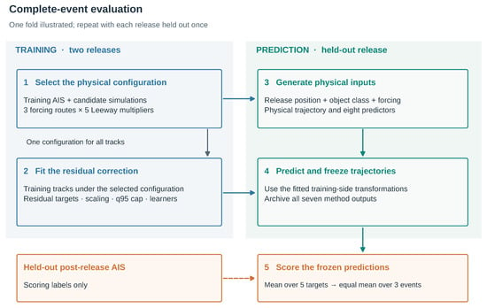
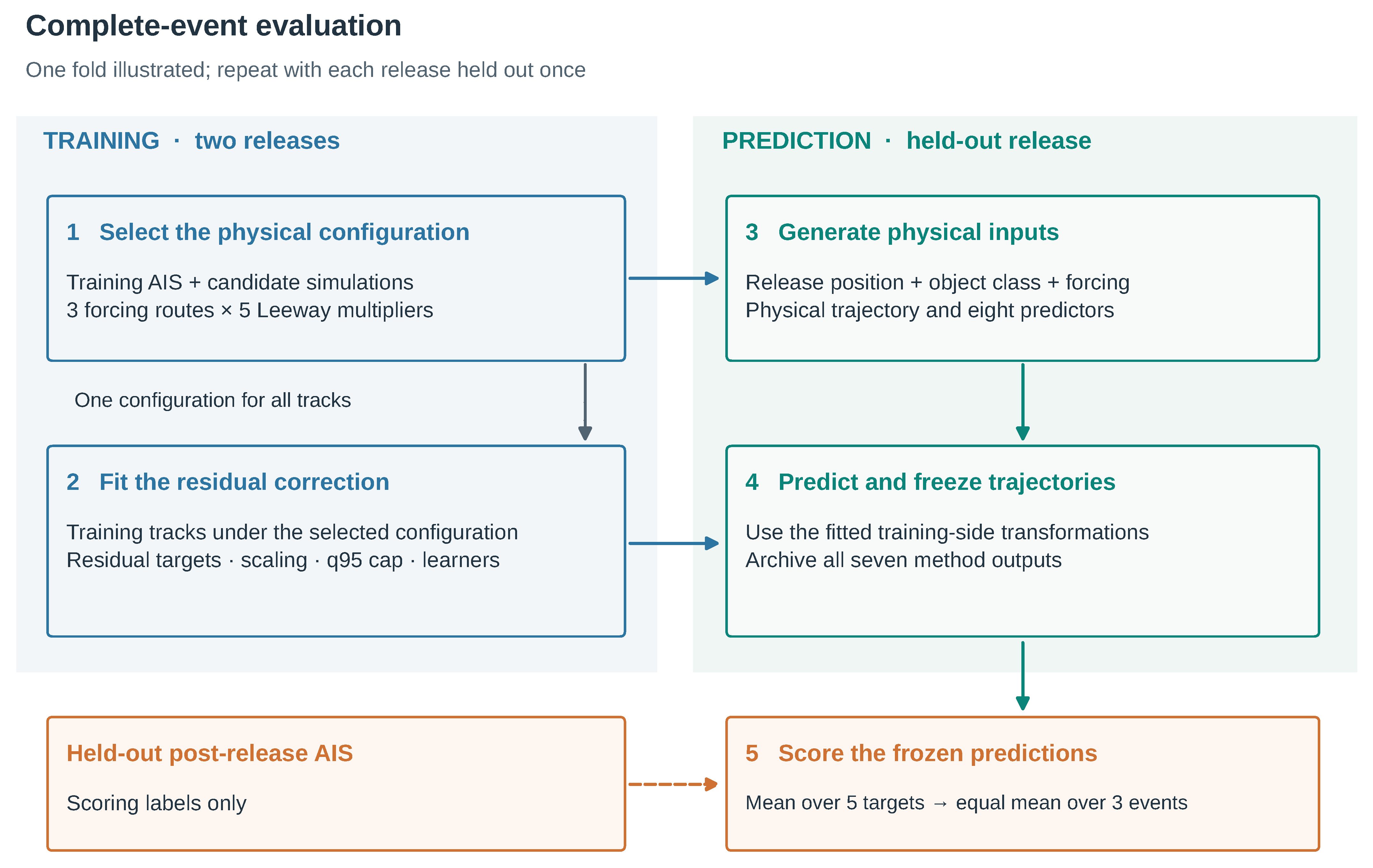
Physical selection and residual estimation are fitted as one prediction procedure. The two training events first rank 15 combinations of forcing route and Leeway multiplier (Section 2.3.3). The selected combination supplies the physical trajectories for both training and prediction within that fold. Consequently, the training labels describe errors of the same physical configuration that will be corrected in the held-out release. Feature scaling, target scaling and the residual-speed cap are then estimated from the training intervals.
The prediction stage uses the release position, release-known object class and environmental inputs to generate the physical baseline and six correction routes (Figure 1). The held-out event’s post-release AIS observations are opened only after the predictions have been generated and archived. Each trajectory starts at its first valid release position; no later observation is used to translate or rotate the prediction.
Figure 1.
Information flow within one complete-event fold. Blue denotes training on two releases, green denotes prediction for the held-out release, and orange denotes scoring after predictions have been frozen. A single training-selected physical configuration supplies both training and held-out trajectories. The dashed orange arrow is the only entry of held-out post-release Automatic Identification System (AIS) data into residual evaluation. Repeat this procedure for each of the three releases.
The evaluation uses three releases that had previously informed method development and is therefore a retrospective assessment of cross-event prediction. The model representation and comparator settings were fixed for the final evaluation, while physical calibration, scaling, residual-speed caps and model fitting were estimated separately within each fold using only the two training releases. This design isolates fitting from the held-out event but does not remove potential optimism arising from earlier methodological choices. Supplementary Section S11 documents the development-stage decisions and fold-specific fitting boundaries.
A configuration is one recurring manikin–equipment state. Its trajectory contains 36 positions and 35 residual intervals over 350 min. The five configurations within a release share an environmental history, so the three releases, rather than the 15 trajectories or 525 intervals, are the independent environmental cases.
2.2. Physics-Anchored Drift Prediction Framework
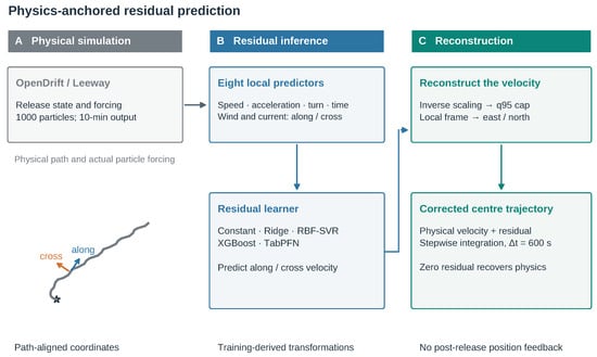
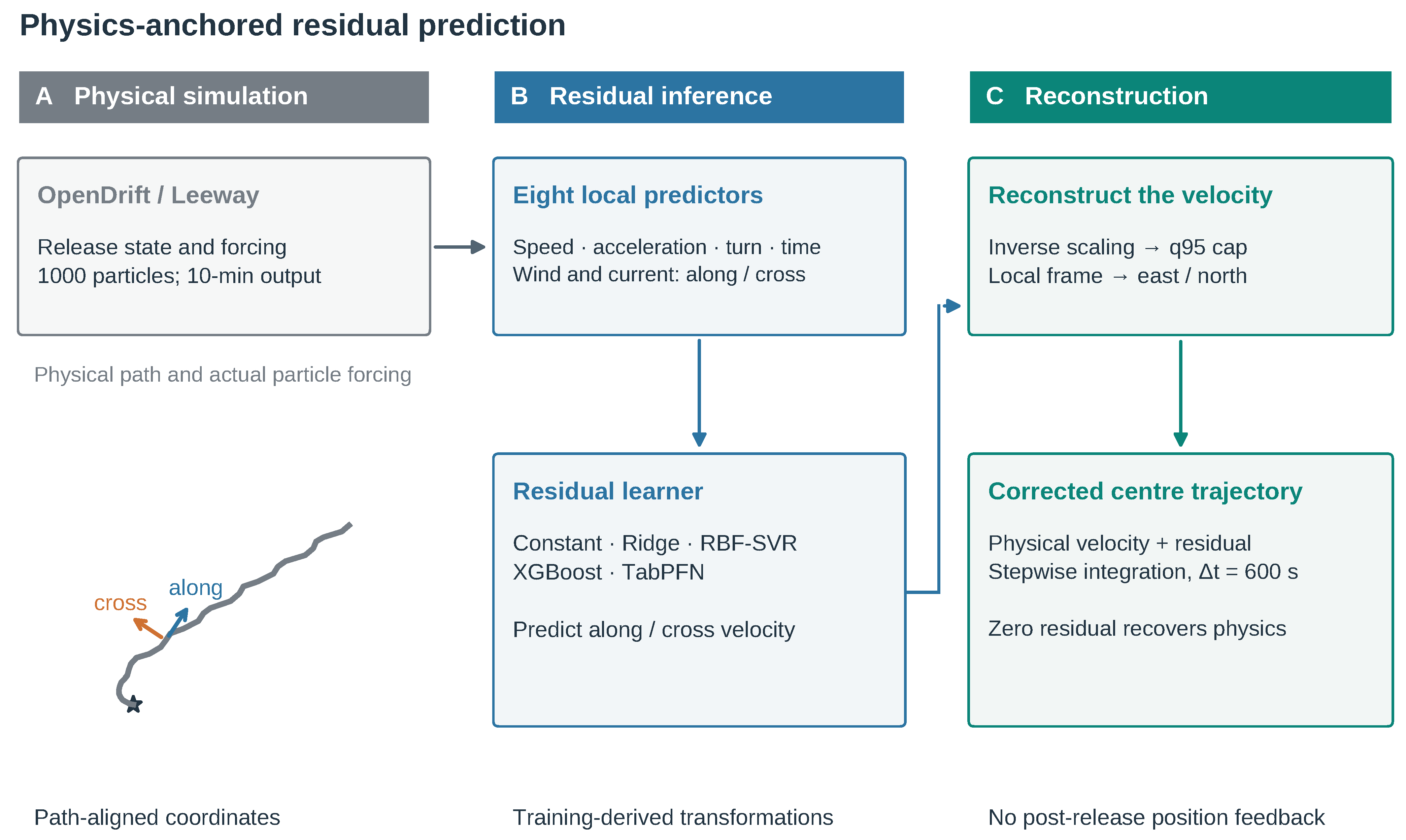
The method adds a conditional velocity correction to an existing physical prediction (Figure 2). Its three stages have distinct roles: the simulation supplies the displacement and local frame, the learner estimates the remaining along-track and cross-track motion, and bounded integration reconstructs the corrected center trajectory. Setting the residual to zero recovers the physical path.
Figure 2.
Physics-anchored prediction in three stages. (A) OpenDrift/Leeway supplies a center trajectory and the particle-level environmental inputs actually used by the simulator. The local-frame inset uses one physical track from the November event; arrows illustrate its tangent and normal directions. The star marks the release origin. TabPFN denotes Tabular Prior-Data Fitted Network. (B) Eight predictors support along-track and cross-track residual-velocity inference. (C) Inverse scaling, a training-derived q95 cap, coordinate rotation and integration yield the corrected trajectory. The selected physical configuration and fitted transformations are fixed before held-out prediction.
2.2.1. Physics-Based Trajectory Anchor
OpenDrift 1.14.10 with the Leeway module simulated 1000 particles within a 50 m release radius, using 5 min Euler integration and 10 min output [2,3,4]. Wind and current were interpolated in space and time. The ensemble mean defined the physical center trajectory , re-anchored to zero displacement at release. Equipment state selected the nearest available PIW class. The joint forcing-route and Leeway-multiplier selection is detailed in Section 2.3.3.
The ensemble-mean path provides a common motion reference for all residual methods. Its position sequence defines the physical comparator, and its interval directions define the moving frame. The experiments evaluate the resulting center trajectories; they do not calibrate the particle spread as a probability region.
2.2.2. Physics-Aligned Residual Inference
For a 600 s interval, physical velocity was
and observed residual velocity was
The velocity residual is projected onto the unit tangent of the physical path and the orthogonal unit normal . A positive tangent component adds speed along the simulated motion; a normal component displaces the target laterally. Because the basis follows the physical path, the two components preserve these meanings through a turn. Resolving the wind and effective current in the same basis gives four environmental predictors. Physical speed, acceleration, the sine of the turning angle and elapsed-time fraction complete the eight-dimensional input. Their means and scales, and those of the two targets, are estimated from the 350 training intervals and then applied unchanged to the query intervals.
The predictors connect the correction to both the simulated motion and the environmental conditions that produced it. Speed and acceleration describe motion magnitude and its change, turning describes path curvature, and elapsed time allows the correction to evolve over the forecast window. Wind and current are averaged from the particle-level variables saved by OpenDrift before projection into the local frame. Using those values preserves the simulator’s environmental inputs and avoids re-interpolating at a mean position that may lie in a masked coastal cell. Absolute position, date, MMSI and event identity are excluded. Even a constant pair of local residual components produces a changing geographic correction when the physical path turns, making the constant-residual control more informative than a fixed east–north offset.
2.2.3. Bounded Trajectory Reconstruction
Predicted residual components were transformed back to east–north coordinates. Their vector magnitude was capped at the 95th percentile of the observed residual-speed distribution in the two training events. Hereafter, q90, q95 and q99 denote caps set to the fold-specific 90th, 95th and 99th percentiles of that training-only distribution; q95 was the primary setting. The cap applies only to the learned residual correction and does not truncate the physical velocity. The corrected trajectory was then integrated as
with the cumulative correction set to zero at release. Capping followed inverse target scaling and preceded integration from the common release origin. It limits single-step correction speed, not physical velocity or total accumulated displacement, and was fixed before the held-out event was predicted.
2.3. Field Data and Environmental Forcing
2.3.1. Dalian Manikin Drift Experiments
Three coastal field experiments near Dalian, China, tracked five recurring manikin configurations over 350 min. Table 2 summarizes their release locations and analysis support. Each trajectory contained 36 positions on a 10 min grid and 35 residual intervals. Thus each event contributed 180 positions and 175 intervals; the complete dataset comprised 540 positions and 525 intervals.
Table 2.
Field events and analysis support. Coordinates approximate the release-location center; intervals and positions are nested observations.
The manikin had an approximate assembled length of 1.80 m and nominal mass of 56 kg. All targets drifted supine. The recurring configurations were no lifejacket, lifejacket, lifebuoy without lifejacket, lifebuoy with lifejacket and immersion suit. They were mapped respectively to OpenDrift PIW classes 1, 2, 1, 2 and 4. Classes 1 and 2 approximate the lifebuoy cases, and class 2 does not reproduce supine posture exactly.
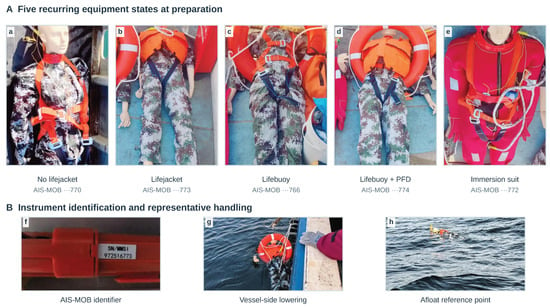
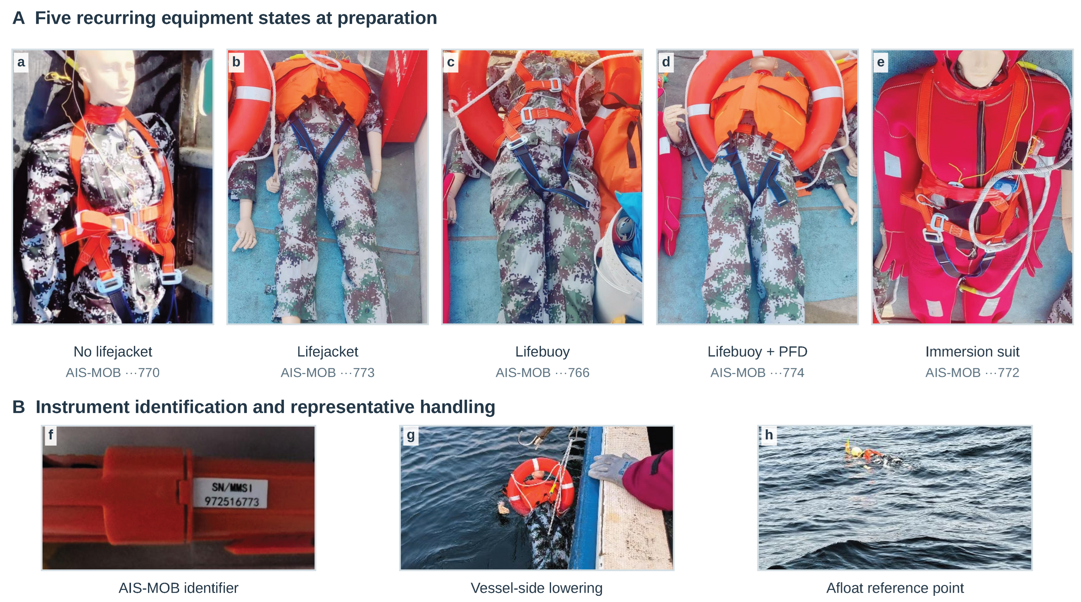
Field preparation linked each equipment state to an AIS man-overboard (AIS-MOB) beacon (AWMOB-100; Shanghai Advanced Avionics Co., Ltd., Shanghai, China) and LED marker before vessel-side lowering (Figure 3). Signals were received aboard the support vessel using an NAR-1000 AIS receiver (New Sunrise Co., Ltd., Suzhou, China). The five beacon identifiers associate the recurring clothing and flotation configurations with their AIS trajectories across releases. This arrangement supports comparisons of equipment states under a shared environmental history.
Figure 3.
Photographic deployment reference for the instrumented manikin configurations. Prepared states: (a) no lifejacket; (b) lifejacket; (c) lifebuoy without lifejacket; (d) lifebuoy with lifejacket; (e) immersion suit. AIS-MOB denotes an AIS man-overboard beacon. PFD denotes personal flotation device (lifejacket); the orange harness in (a) is not a lifejacket. The three-digit suffixes identify the corresponding AIS-MOB units, whose full identifiers recur in the three event logs. (f) Example of a beacon label; (g) vessel-side lowering; (h) an afloat target. The observed AIS track refers to the instrument mounted near the head, not the manikin center of mass.
The AIS-MOB position refers to the instrument mounted near the head. The configuration descriptions and identifier mappings are listed in Supplementary Table S8. Equipment state determines the physical object class but is not an additional predictor in the primary residual model; the historical configuration-indicator comparison is in Supplementary Section S2. These repeated states allow matched within-event comparisons under common forcing. The drifting targets were manikins, with no human participant or live animal used as a target.
2.3.2. AIS Processing
Raw AIS logs were decoded from NMEA !AIVDM messages. Dynamic position reports of types 1–3 and 18–19 were retained. Invalid coordinate sentinels, coordinates outside geographic bounds, unparseable timestamps and duplicate timestamps were removed. China Standard Time was converted to UTC. Each irregular trajectory was linearly interpolated onto a 10 min grid anchored at its first valid report, without smoothing or extrapolation. All tracks contained 36 finite positions and 35 residual intervals through 350 min. WGS84 coordinates were converted around each release point using m per degree longitude and 110,540 m per degree latitude; then they were re-anchored at .
The raw AIS cadence was usually much finer than the analysis grid: the median positive interval was 3 s, the interquartile range was 3–4 s and the 95th percentile was 40 s; 85.1% of intervals were at most 10 s. Outages were less frequent but much longer, with a maximum bracketing gap of 17,694 s. Of the 540 grid positions, 77 lay inside gaps exceeding 600 s and 65 inside gaps exceeding 1200 s. Linear interpolation connects the reported endpoints and can smooth turns or velocity changes inside an outage. Such positions are estimated reference locations, and their displacement differences also enter the residual targets. We therefore examine the training-label distribution and repeat fitting and scoring after joint gap exclusion, rather than treating a change in scoring support alone as a test of label reliability.
Long bracketing gaps were concentrated in November and May. At a 20 min threshold, 28/180 November positions and 37/180 May positions were flagged, compared with none in April. At least one endpoint was flagged in 35/175 November intervals and 43/175 May intervals. A direct overlap check identified no additional intervals beyond this endpoint rule. No training-target exclusion was applied in the primary analysis; joint exclusion at 20 and 60 min thresholds was evaluated separately (Section 2.5.2 and Supplementary Section S9).
2.3.3. Environmental Forcing Data
The forcing combines archived products. ERA5 supplied hourly 10 m wind on a 0.25° grid [17]; archived Integrated Forecasting System (IFS) 10 m wind came from 0 UTC cycles initialized one day before release, with 3 h output on the same grid spacing. Copernicus Marine supplied approximately 1/12° hourly surface fields. Non-tidal circulation came from cmems_mod_glo_phy_anfc_0.083deg_PT1H-m; tide, Stokes drift and merged total current came from cmems_mod_glo_phy_anfc_merged-uv_PT1H-i, at 0.494 m. Component configurations summed circulation, tide and Stokes drift; the merged configuration used total current alone. References [18,19] describe the separate Global Drifter Program (GDP)-source reanalysis products. Supplementary Section S15 distinguishes valid times, forecast initialization, product issue times and acquisition evidence. Copernicus production issue times and prediction-origin availability are not established by the retained files; the evaluation characterizes archived forcing.
The physical search crossed three forcing routes with five Leeway multipliers, giving 15 candidates (Table 3):
Table 3.
Candidate environmental-forcing routes and Leeway multipliers.
No components were added to an already merged current. Candidate simulations used the same particle number, release radius, integration settings and random seed (42). Multipliers scaled the Leeway contribution, so a zero value suppressed that contribution without removing the supplied current.
Candidates were ranked on the two outer-training events using, in order, direction-gate pass count, mean endpoint direction error, mean log-length-ratio penalty, mean normalized cumulative Lagrangian separation (NCLS) skill and the mean average displacement error (ADE). Route name and multiplier resolved remaining ties. The direction gate required endpoint direction error below 90° and positive mean step-velocity cosine; the length penalty summed absolute logarithms of net-displacement and path-length ratios. Higher gate counts and skill were preferred, and lower errors and length penalties were preferred. The physical ranking used the first 37 output positions through 360 min, following the preceding physical study; residual fitting and final comparisons used 36 positions through 350 min. Both windows were confined to training events during selection.
The direction-first rule selected H3 with multiplier 0.00 for F1 and H2 with multiplier 1.00 for F2 and F3. A multiplier is selected for a particular environmental-product and target-model combination: zero removes parameterized Leeway while retaining the supplied current, rather than measuring physically absent windage. Wind speed and wind–current alignment, and compensation between forcing error and target response, can affect the preferred combination. We examine this dependence with a fixed-route scan of all five multipliers and with alternative training-only selection rules followed by residual refitting (Section 3.4). Complete training rankings appear in Supplementary Table S6.
The residual represents the net motion error remaining after the physical simulation, including environmental-product error, unresolved coastal flow, imperfect target response and observation processing. Learning this aggregate quantity makes the correction directly compatible with velocity integration; its individual values are not identified force coefficients.
2.4. Residual Learning and Inference
All correction methods used the same outer folds, eight predictors, target scaling, training-derived speed cap and coordinate integration. The constant residual broadcast the mean standardized training residual. The ridge residual used fixed . The radial-basis-function support vector regression (RBF-SVR) residual used separate regressors implemented in scikit-learn 1.6.1 for the two residual components with fixed C = 1.0, epsilon = 0.1 and gamma = scale.
The TabPFN residual used TabPFN 2.2.1 with random state 20260906 and otherwise default regressor settings; separate pretrained regressors predicted the two components without parameter fine-tuning or Dalian-based hyperparameter selection. A stability analysis repeated the same fixed pipeline with random states 20260900–20260909. These runs were retained individually rather than selected or ensembled.
The extreme gradient boosting (XGBoost) residual used XGBoost 3.0.5 and supplied a strong tree-ensemble comparator. Within each outer fold, its small grid crossed maximum depths 2 and 3, learning rates 0.03 and 0.1, and minimum child weights 5 and 20 while fixing 200 trees, subsample and column-subsample fractions at 0.8 and L2 regularization at 10. The two outer-training events were exchanged as inner train and validation events; mean 350 min validation-event ADE selected one setting before refitting on both training events. The outer held-out event was not used for this selection. The physical configuration stayed fixed during inner learner tuning, having been selected using both outer-training events. Thus inner validation scores were conditional on that physical selection; the physical search was not repeated using only the single inner-training event.
Numerical processing used NumPy 2.2.6 and pandas 2.3.3, and the regression pipeline used PyTorch 2.12.0. The revision analyses ran in Python 3.13.9; figures were generated using Matplotlib 3.10.8.
The hierarchy of comparators separates the sources of predictive benefit. Physics supplies the uncorrected trajectory; the constant control transfers its mean local velocity error; Ridge, RBF-SVR, XGBoost and TabPFN allow the correction to depend on the same eight predictors. The fixed settings and inner-tuned XGBoost grid represent different specified implementations rather than equal tuning budgets. TabPFN uses the training table as context for an existing pretrained regressor, so the methodological contribution is the physical reference and residual prediction procedure.
The fixed equal-weight fusion averaged ridge and TabPFN coordinates:
Equal fusion tests whether the linear and TabPFN corrections complement one another at trajectory level. Its weights remain one half for every event and time, without observation-dependent selection.
2.5. Evaluation Design
2.5.1. Experimental Comparisons
The experiments test three linked propositions: conditional learning adds accuracy beyond mean-bias transfer; the moving representation contributes to that gain; and the result persists when observation support, physical selection or inference seed changes. All seven primary routes use the same recalibrated CELO predictions. The matched coordinate controls use the same folds and physical anchors. Gap exclusion, alternative selection and inference-seed experiments each vary a defined part of the pipeline while retaining the corresponding matched constant control.
Supplementary analyses examine tide completion, the effect of shared-event training and testing, and representation transfer from Global Drifter Program (GDP) observations [20]. These analyses use different physical configurations and provide methodological context rather than estimates of performance for the primary CELO procedure.
2.5.2. Evaluation-Boundary and Robustness Diagnostics
A supplementary split diagnostic compares complete-event holdout with whole-trajectory splits that share release events between training and testing (Supplementary Section S6.1). It evaluates the effect of shared environmental histories on apparent prediction accuracy using a common physical configuration across splitting strategies.
Residual behavior was characterized by differencing the cumulative correction between the TabPFN and physical trajectories over each 600 s interval and projecting the resulting velocity onto the physical tangent frame. Comparing its magnitude with the fold-specific q95 cap identifies whether clipping contributes to the trajectory differences.
The AIS-gap sensitivity used 20 min as the primary threshold and 60 min as a supplementary threshold. A residual interval was removed from fitting when either endpoint lay within a raw-report gap exceeding the threshold; an explicit interval-overlap check produced no further removals. Feature and target scaling, the constant residual, the q95 cap and TabPFN fitting were then recomputed from the retained intervals. At scoring, positions affected by the same threshold were masked before trajectory-, event- and macro-averaging. This joint procedure was applied to the physical, constant-residual and TabPFN methods. A scoring-only calculation using the frozen primary predictions was retained to distinguish a change in evaluation support from a change in fitted residuals.
To distinguish a change in residual labels from the effect of refitting, we also compare the unscaled, unclipped training residuals while holding each fold’s physical trajectories fixed. For each gap threshold, the retained along-track and cross-track components and their vector magnitudes are summarized by sample count, mean, sample standard deviation and distribution quantiles. Section 3.4 reports the speed distributions, while the joint-exclusion experiment evaluates whether the fitted correction remains useful on the corresponding scoring support.
Physical-selection sensitivity first compared the primary winners with their nearest candidates and repeated ranking after rounding direction error to 0.1°. Two prespecified alternatives were propagated through residual fitting: a 0.5° direction-tolerance rule that used ADE within the tolerance set, and a rule that ranked direction-gate count before ADE. Both used training events only. TabPFN seed stability held the selected physical trajectories, folds, features and evaluation procedure fixed while repeating inference for ten predetermined random states. Seed summaries are descriptive technical-repeat statistics; they do not add environmental replications.
A separate Leeway scan isolates the trajectory response to the multiplier itself. Within each fold, the selected forcing route, particle setup and simulation seed are held fixed while the multiplier takes values of 0, 0.25, 0.50, 0.75 and 1.00. Physical-trajectory ADE and the distance between zero- and unit-multiplier endpoints are evaluated over 350 min. This scan describes sensitivity of the physical path; the alternative-selection experiments instead evaluate the complete correction procedure after both the anchor and residual fit change.
For descriptive event characterization, saved particle-level wind and effective-current vectors were ensemble-averaged for the five held-out physical simulations for each event over 350 min. We summarized speed, vector-mean bearing, wind–current angle and temporal variation. The cached effective current does not separately identify tide and Stokes contributions, so no component-specific statistics were inferred. These 180 path-time samples per event describe the forcing presented to the model; they do not add independent events or establish broad sea-state coverage.
The matched coordinate experiment distinguishes target representation from environmental-feature representation. LOCAL retains the along-track and cross-track predictors and targets. TARGET-EN retains the eight local predictors but learns east–north targets. ALL-EN also expresses the four wind/current predictors in east–north coordinates, while retaining physical speed, acceleration, turning and elapsed time. Each arm uses TabPFN 2.2.1, its own training-only component means and scales, the same rotation-invariant q95 speed cap, and the same integration and scoring. The primary seed 20260906 and endpoint seeds 20260900 and 20260909 of the existing ten-seed set are matched across arms. All nine predictions within a fold are saved before its scoring observations are opened. Rotations depend exclusively on the physical tangent.
2.5.3. Evaluation Metrics
Average displacement error (ADE) and final displacement error (FDE) were the primary metrics. Endpoint direction error and a bounded trajectory skill derived from normalized cumulative Lagrangian separation were secondary metrics. Following Liu and Weisberg [21], cumulative pointwise separation was normalized by the corresponding cumulative observed trajectory length. We used their bounded skill form with threshold parameter , and refer to it below as the NCLS skill:
where is the observed trajectory length accumulated from release through time t. The unclipped normalized cumulative separation increases with error; the reported bounded skill decreases from 1 toward 0 and is clipped at zero once normalized separation reaches or exceeds 1. Metrics were calculated at 60, 180 and 350 min, averaged first across five configurations within each event and then equally across events. With , inferential p values were not computed from the 15 nested trajectories or 525 residual intervals. Supplementary trajectory-shape diagnostics include mean step-direction cosine, reverse-step fraction, displacement and path-length ratios, discrete Fréchet distance and maximum separation.
ADE summarizes separation over the available path and is the primary measure of center-trajectory accuracy. FDE emphasizes accumulated endpoint error and can expose late divergence that is diluted in ADE. Endpoint direction error evaluates the bearing of net displacement, while the NCLS skill compares cumulative separation with the time-matched accumulated observed length. No single metric is sufficient: a method can improve mean separation while distorting direction or path length. Model ranking was therefore based on the joint metric pattern, with event-wise ADE used to identify whether a macro gain depended on one favorable event.
All improvements are descriptive. We paired method-specific ADE by event and configuration, reporting difference medians and the number of improving pairs. A leave-one-configuration analysis omitted the same configuration from all three events and recalculated macro ADE without refitting. A conditional bootstrap drew five configuration identities with replacement 1000 times (NumPy seed 20260920), retaining each identity across all three fixed events. The same draws were used for every method and paired difference. Reported 2.5th–97.5th percentile ranges measure sensitivity to configuration composition, not confidence intervals for future events. Likewise, the mean, sample standard deviation and range across TabPFN seeds quantify software-level inference variability, not sampling uncertainty for future releases. No significance tests treated trajectories, intervals or seeds as independent environmental events.
2.5.4. Controlled Observation Gaps and Fixed-Radius Inclusion
To measure interpolation effects against observed motion, we introduce artificial gaps into densely reported portions of the original tracks. Candidate windows start every 10 min within the 350 min analysis period and span 20, 60 or 120 min. A window is eligible when its largest original reporting interval is at most 60 s; a 120 s criterion tests sensitivity to this definition. We retain the two raw reports bracketing the window, remove the intervening reports and reconstruct positions linearly. Position errors are evaluated at interior 10 min grid points against the dense-reference trajectory. The error in a 10 min residual-velocity target is the difference between reconstructed and reference displacement increments divided by 600 s: the common physical increment cancels, and its vector norm is invariant to rotation into the moving frame. We average windows within each trajectory, available trajectories within each release, and then releases equally. Overlapping windows are descriptive repeated tests of the recorded motion.
For a direct geometric interpretation of prediction error, we also evaluate whether each reference position lies within 500, 1000 or 2000 m of the frozen predicted center. These radii are specified before computing the diagnostic. Inclusion is reported at 60, 180 and 350 min and averaged over 10–350 min, excluding the shared initial position. Aggregation gives equal weight to configurations within releases and then to available releases. We repeat the calculation after excluding positions bracketed by raw gaps longer than 20 min. This measures inclusion within fixed distances; it does not fit a probabilistic search region or simulate detection.
3. Results
3.1. Accuracy Beyond Mean-Bias Correction
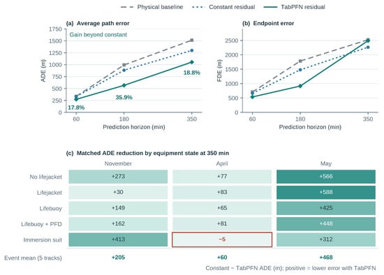
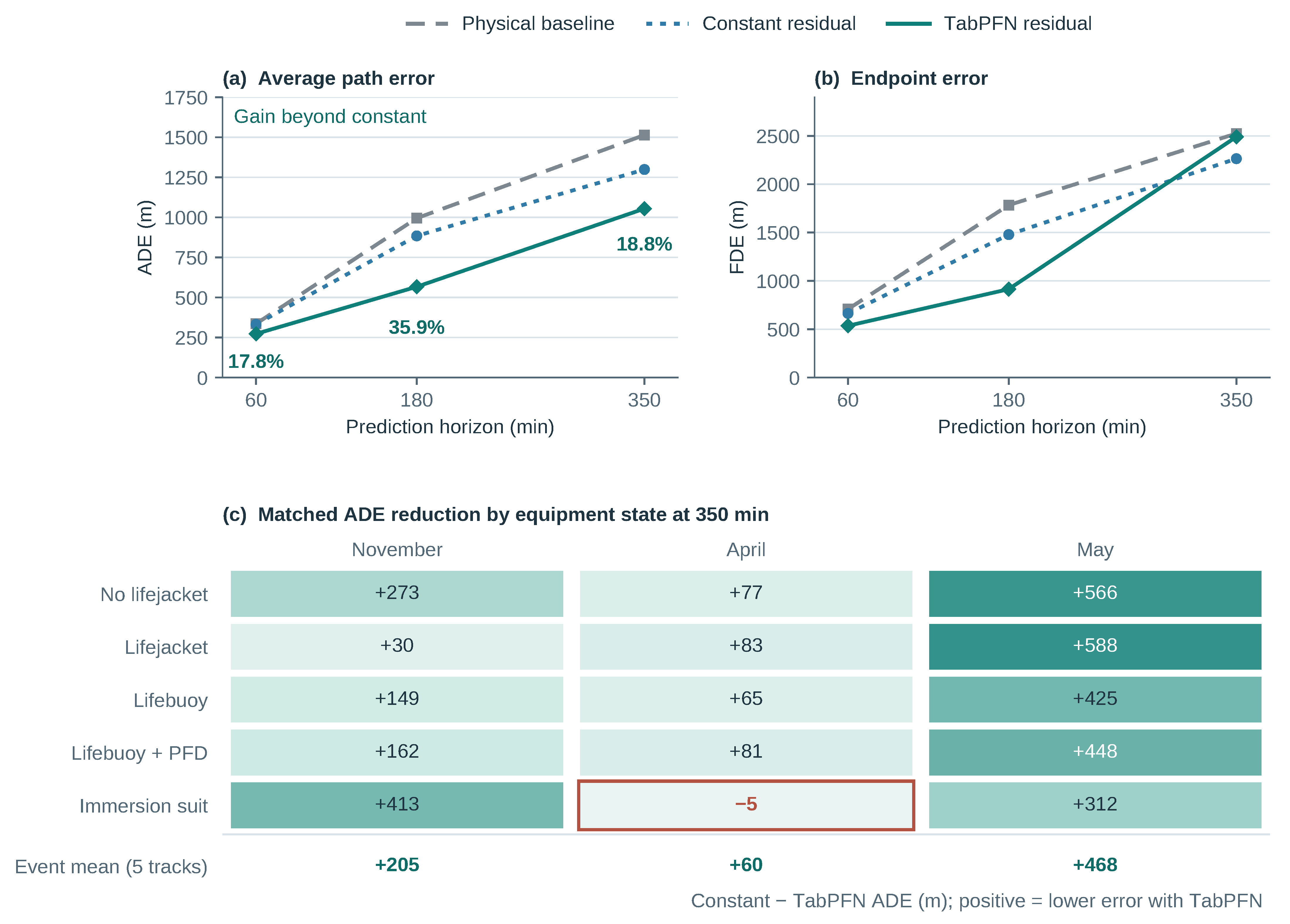
The physical, constant-residual and TabPFN predictions form a direct decomposition of the correction benefit (Table 4). At 180 min, the physical ADE of 994.8 m falls to 884.4 m after mean-bias correction and to 566.8 m after conditional correction. Thus TabPFN adds a 317.6 m reduction beyond the constant control, or 35.9%. At 60 and 350 min, the additional reductions are 59.2 and 244.4 m, respectively. Conditional information improves average path placement at all three reported horizons.
Table 4.
Incremental average displacement error (ADE) decomposition after outer-fold physical selection. Percentages use constant residual ADE as the denominator.
The 180 min result is supported by the other trajectory measures (Table 5). TabPFN has the lowest FDE, 914.3 m, and endpoint direction error, 25.3°, together with the highest NCLS skill, 0.474. The improvement therefore combines closer intermediate positions with a closer endpoint and better overall direction. Figure 4 shows how the gain changes with prediction time. By 350 min, TabPFN still has the lowest ADE, 1054.4 m, compared with 1298.8 m for constant correction and 1514.0 m for physics. Its direction error is 5.8° and NCLS is 0.678. Constant correction, however, gives the closer terminal position: 2264.3 m FDE versus 2490.5 m, a difference of 226.2 m or approximately 10.0%. The distinction is between improved placement over the path and improved position at its last time.
Table 5.
Event-macro performance after outer-fold physical selection. ADE and FDE denote average and final displacement error; NCLS denotes normalized cumulative Lagrangian separation skill. Downward arrows indicate that lower values are better, and upward arrows indicate that higher values are better. Bold denotes the lowest error or highest NCLS within each horizon; all means give equal weight to three events.
Figure 4.
Prediction-horizon and event-level gains in the primary complete-event leave-one-out (CELO) experiment. (a) Event-macro average displacement error (ADE) at all three reported horizons; annotations give the additional reduction from constant correction to TabPFN. (b) Event-macro final displacement error (FDE) for the same predictions, showing the reversal of the constant–TabPFN ordering at 350 min. Color and line style identify methods consistently in both panels. (c) Matched constant-minus-TabPFN ADE reduction for each recurring equipment state and release at 350 min (m). Positive values favor TabPFN; the outlined April immersion-suit cell is the sole reversed pair. The bottom row gives the mean across five configurations within each event. These 15 cells are descriptive comparisons nested within three releases, not 15 independent environmental tests.
3.2. Transfer Across Releases and Equipment Configurations
The primary mean-bias-to-conditional improvement appears in each of the three held-out releases (Table 6): 205.4 m in November, 60.0 m in April and 467.8 m in May. The largest additional gain occurs in May, where the physical ADE is also largest. April starts with smaller physical and constant-correction errors and provides a narrower margin for improvement. Across the 15 matched event–configuration pairs, TabPFN improves 14 relative to constant correction and all 15 relative to physics. The median TabPFN-minus-constant difference is −161.7 m; omitting any one recurring configuration leaves macro ADE between 1038.4 and 1062.2 m. The aggregate gain consequently extends across the recurring equipment states rather than depending on one state alone.
Table 6.
Event-wise 350 min ADE (m) after outer-fold physical selection. Bold denotes the lowest value within each row.
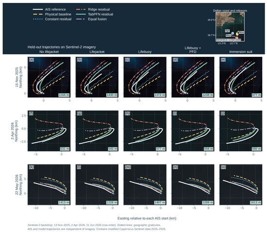
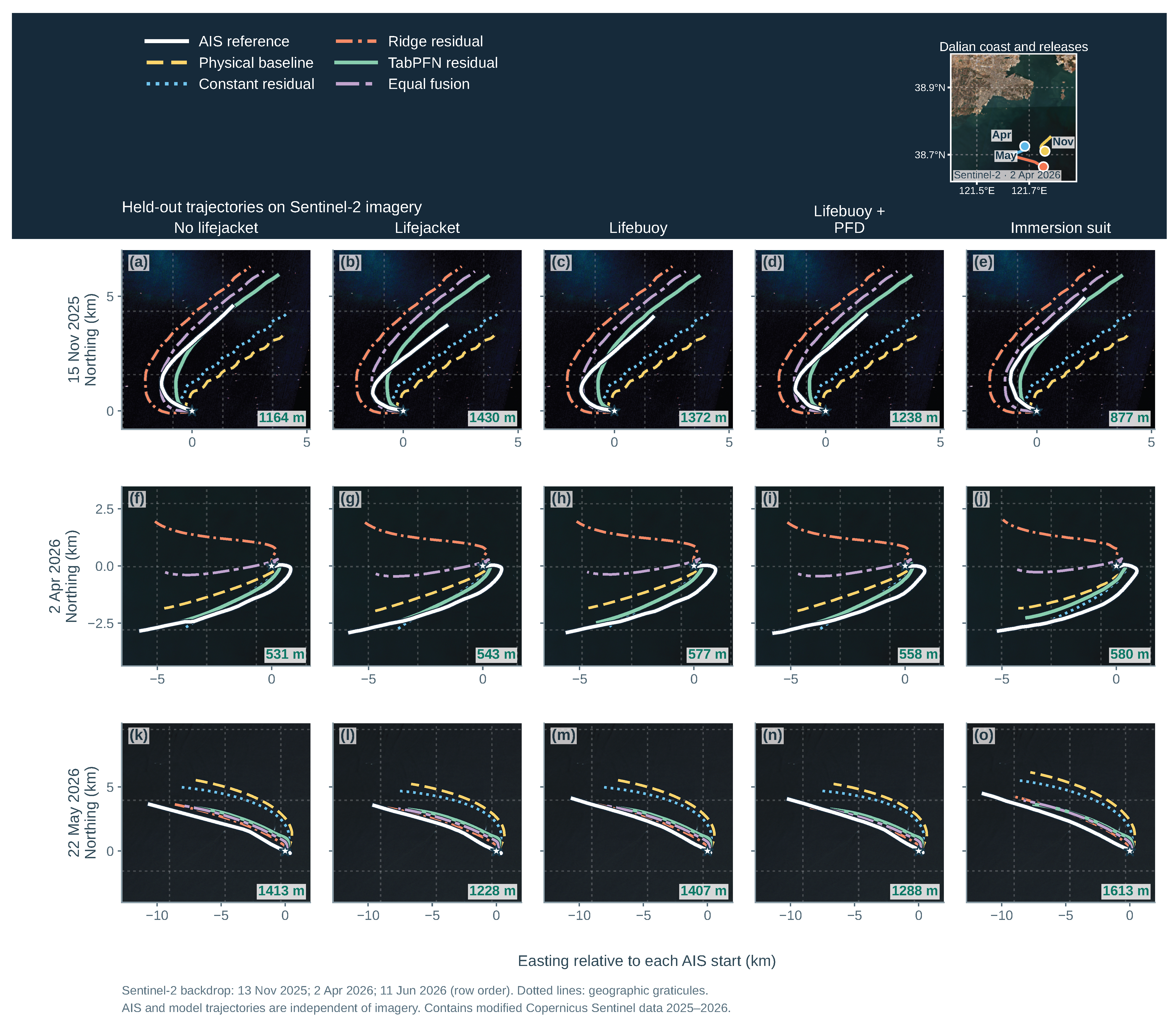
The trajectory overlays connect these summaries to the predicted paths (Figure 5). Different regressors can be useful in different releases: Ridge attains the lowest May ADE, 838.0 m, but gives 2442.9 m in April, while equal fusion has the lowest November ADE, 1036.8 m. Averaging Ridge and TabPFN retains part of Ridge’s April displacement, producing 1412.0 m ADE there. TabPFN gives the lowest April and overall macro ADE among the primary methods. These comparisons show why the benefit of a conditional correction must be examined across releases as well as in aggregate. Configuration-resampling results, which retain the same three environmental histories, are provided in Supplementary Section S8.
Figure 5.
AIS reference and recalibrated complete-event-held-out trajectories for all 15 targets over georeferenced Sentinel-2 imagery. Panels (a–e) show 15 November 2025: (a) no lifejacket, (b) lifejacket, (c) lifebuoy, (d) lifebuoy with lifejacket and (e) immersion suit. Panels (f–j) show 2 April 2026 with the same configurations: (f) no lifejacket, (g) lifejacket, (h) lifebuoy, (i) lifebuoy with lifejacket and (j) immersion suit. Panels (k–o) show 22 May 2026: (k) no lifejacket, (l) lifejacket, (m) lifebuoy, (n) lifebuoy with lifejacket and (o) immersion suit. White solid: AIS reference; yellow dashed: physics; blue dotted: constant residual; orange dash-dot: ridge; mint solid: TabPFN; purple long-dash-dot: equal fusion. Stars mark release origins; numbers report the TabPFN ADE over 350 min. Thin dotted lines are geographic graticules at 0.025° intervals in November and April and 0.05° in May. Axes retain equal local east–north scale and identical limits within each release. The inset shows the Dalian coast and one representative AIS track per release on a 2 April 2026 Sentinel-2 image. Main-panel satellite scenes were acquired on 13 November 2025, 2 April 2026 and 11 June 2026, respectively. They provide geographic context only, are not observations of the drifting targets and were not used for model fitting or evaluation; in particular, the May backdrop was acquired 20 days after that release. The November backdrop was contrast-enhanced for display. Contains modified Copernicus Sentinel data 2025–2026. PFD denotes a personal flotation device (lifejacket).
3.3. Contribution of the Moving Coordinate Representation
The coordinate controls isolate a component of the proposed method rather than introduce another learner (Table 7). Keeping the local predictors but replacing the along-track and cross-track targets with east–north targets raises 180 min ADE from 566.8 to 1263.1 m. Expressing the environmental predictors in east–north coordinates as well gives 1086.0 m. At 350 min, the corresponding ADEs are 1054.4, 1525.1 and 1542.3 m. The physical anchors, training support and regressor are shared, so these differences support the role of the moving representation in the tested prediction procedure.
Table 7.
Matched coordinate ablation with seed 20260906. All arms share physical anchors, folds, predictor information, reconstruction and scoring; scaling is fitted in the relevant coordinate system. Errors are equal-event means in meters.
The 180 min advantage is present in each release, not just in the macro average. Moving-frame ADEs are 523.3, 439.5 and 737.5 m for November, April and May, respectively; the corresponding east–north-target values are 1250.4, 1335.4 and 1203.6 m, and the fully east–north values are 617.4, 1486.8 and 1153.6 m. Thus, keeping the same physical motion and regressor while changing the coordinate representation affects transfer across all three environmental histories at this horizon. The component-wise scaling is fitted within each representation, so the comparison tests the coordinate-based prediction procedure as a whole.
The moving frame retains lower macro ADE than both controls in all nine matched seed–horizon comparisons. The endpoint ordering is different at 350 min: TARGET-EN and ALL-EN yield FDEs of 1722.0 and 2258.9 m, both below LOCAL at 2490.5 m. Coordinate choice therefore affects how error is distributed along the reconstructed path, rather than providing an advantage in every measure. All three seeds and every event-level result are retained in Supplementary Tables S26 and S27. No prediction in the coordinate experiment activates the q95 cap, so active clipping does not account for the observed differences.
3.4. Dependence on Observation Support and Physical Selection
Joint gap exclusion preserves the macro advantage over constant correction while changing both the labels available for fitting and the positions available for scoring. At the 20 min threshold, physics, constant correction and TabPFN have matched-support ADEs of 1480.1, 1361.2 and 1165.1 m, respectively, giving a 14.4% conditional gain. At 60 min, the values are 1481.5, 1310.6 and 1038.4 m, giving 20.8%. The respective scoring supports are 475 and 520 of the original 540 positions. Relative gains are compared within each support rule; the absolute ADEs across rules do not use identical reference positions.
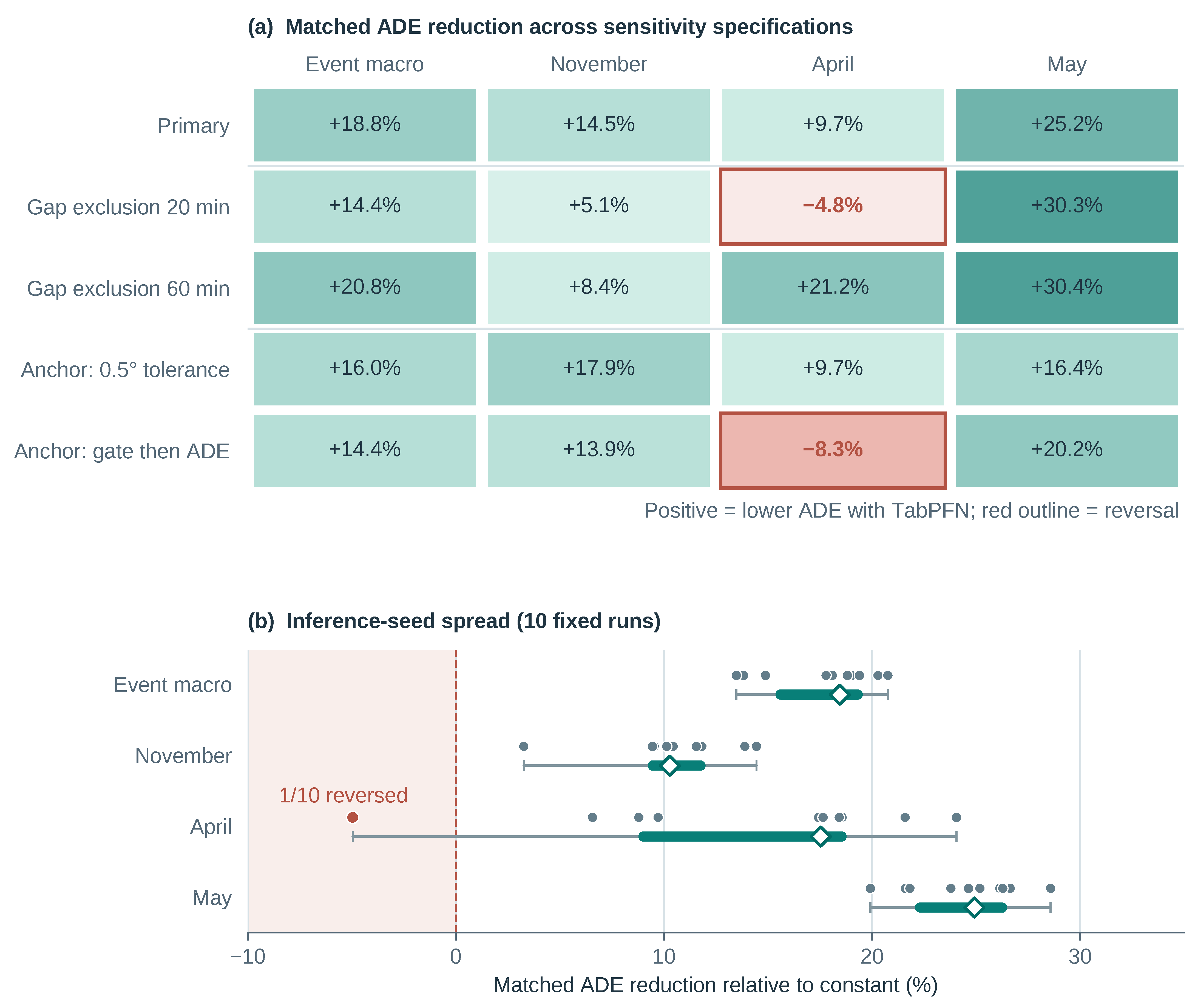
The event-level comparison identifies where that robustness comes from (Table 8). November and May retain positive increments over constant correction at both thresholds, and all three releases improve at 60 min. At 20 min, the April ADE changes from 747.9 m for constant correction to 784.0 m for TabPFN, while all 180 April scoring positions remain available. The changed outcome therefore reflects the residual fit learned from November and May rather than removal of April observations. Taken together with the label distributions, these results show that the macro gain survives removal of long-gap labels, while the smaller April increment depends more strongly on which training intervals are retained.
Table 8.
Joint training-and-scoring gap exclusion at 350 min. All methods use the same scoring positions within each threshold. ADE and gains are in meters; positive gains indicate lower ADE for TabPFN than for constant correction. Event macro averages the three event means equally.
Table 9 examines what changes in the training labels before refitting. At 20 min, F1 retains 307 of 350 intervals and its speed P95 falls from 0.564 to 0.500 m s−1, whereas its mean changes little. F2 retains 272 intervals with a similar P95 but a higher P99, from 0.461 to 0.477 m s−1. F3 retains 315 intervals and its mean decreases from 0.164 to 0.161 m s−1. Excluding long-gap labels therefore changes sample composition and distribution tails differently across folds. These fixed-anchor statistics separate the label change from the simultaneous refitting of scaling, mean residual, speed cap and regressor in the joint-exclusion experiment. They do not recover the unobserved path inside an actual outage.
Table 9.
Residual-speed distributions before scaling or clipping, with physical anchors held fixed. The threshold excludes training intervals affected by longer AIS gaps. The full along-track, cross-track and event-specific statistics are in Tables S21 and S22.
The physical configuration also affects the correction task. With the forcing route fixed, scanning the original five Leeway multipliers gives markedly different trajectory responses across releases (Table 10). November ADE ranges from 1543.7 to 1892.0 m, and May ADE from 2210.2 to 2401.6 m. April ADE stays near 785–788 m even though changing from zero to unit scaling moves its mean endpoint by 492.4 m. Similar path-averaged error can thus coexist with substantial endpoint movement. These held-out scans describe sensitivity; they do not replace the training-selected configuration. The full scans and training rankings appear in Supplementary Section S13.
Table 10.
Physical-trajectory sensitivity to Leeway scaling at 350 min. Each fold retains its selected forcing route while the multiplier varies over 0, 0.25, 0.50, 0.75 and 1.00. Endpoint movement is the mean distance between zero- and unit-scaling predictions, not endpoint error.
The full refitting comparisons address the practical consequence of choosing a different physical anchor. Under the direction-tolerance rule, the physical, constant-residual and TabPFN macro ADEs are 1553.4, 1388.0 and 1166.3 m; under gate-then-ADE selection they are 1641.6, 1516.2 and 1298.3 m. Conditional correction therefore removes a further 221.7 and 217.9 m beyond the matched constant controls. The persistence of this increment across distinct selected configurations supports a correction benefit that is not tied to one exact Leeway choice.
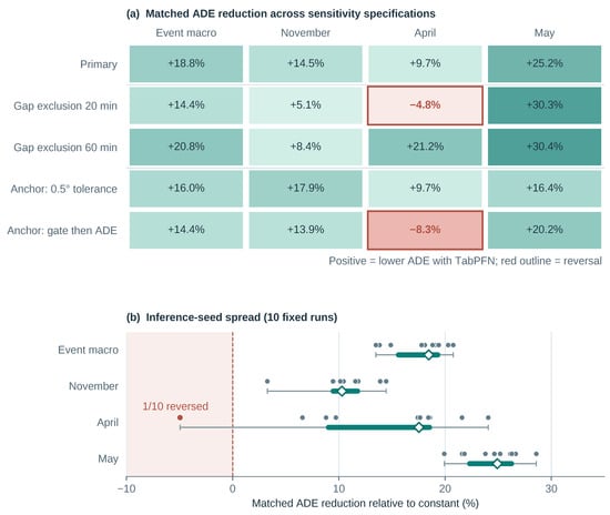
Alternative training-only physical-selection rules retain macro increments of 16.0% and 14.4% beyond constant correction after residual refitting. Across ten fixed TabPFN seeds, 350 min macro ADE has mean 1069.7 m, sample standard deviation 34.3 m and range 1029.1–1123.7 m; every run improves the constant macro score. Figure 6 brings these checks together. November and May retain positive increments throughout. April reverses under 20 min gap exclusion (784.0 versus 747.9 m), gate-then-ADE physical selection (584.0 versus 539.2 m) and seed 20260900 (648.2 versus 617.6 m). All April scoring positions remain available under gap exclusion, so that reversal follows changes in the November/May training support and resulting fit.
Figure 6.
Robustness of the 350 min gain over matched constant correction. (a) Percentage ADE reduction for the event macro and each held-out release under the primary analysis, both joint training-and-scoring AIS-gap exclusions and two alternative physical-selection rules. Each cell uses that specification’s matched constant control; outlined cells mark April reversals. The macro percentage is the reduction in equal-event mean ADE, not the mean of the three event percentages. (b) Ten fixed TabPFN inference seeds shown separately for the same four aggregates. Dots are individual runs; thin lines span the observed minimum and maximum, thick segments the 25th–75th percentiles, and diamonds the medians. The red dot is the sole seed-level reversal (April, seed 20260900). These are descriptive spreads, not confidence intervals or independent releases. Gap thresholds change scoring support, so absolute ADEs across specifications are not directly comparable.
The primary predicted correction speeds remain below their training caps: maxima of 0.428, 0.198 and 0.267 m s−1 versus caps of 0.564, 0.372 and 0.293 m s−1. None of the primary or ten-seed TabPFN predictions is clipped. Together, the support, anchor and seed checks establish a persistent macro path-accuracy gain, with a smaller and less stable additional margin in April.
3.5. Observed Interpolation Error and Geometric Inclusion
The artificial-gap experiment measures how interpolation changes both positions and residual targets (Table 11). Across the three releases, mean position error rises from 31.1 m for a 20 min gap to 92.0 m for 60 min and 244.8 m for 120 min. Mean residual-velocity error rises from 0.053 to 0.090 and 0.127 m s−1. The 120 s eligibility criterion gives corresponding position errors of 32.5, 89.3 and 246.5 m. Thus interpolation error grows appreciably with gap duration in the observed dense segments. Together with the joint fitting-and-scoring exclusion results, this provides two complementary checks: direct measurement of interpolation distortion and assessment of the model gain when long-gap labels are removed. The experiment tests observed motion hidden artificially, rather than reconstructing the unknown motion during actual multi-hour outages.
Table 11.
Artificial-gap reconstruction errors under the 60 s dense-reference criterion. Means are averaged within trajectories and then equally across releases. Windows overlap; their counts are not independent event sample sizes. All three releases contribute at every duration.
The fixed-radius diagnostic connects the trajectory comparison to a concrete distance around the predicted center (Table 12). At 180 min and a 1000 m radius, TabPFN includes 66.7% of reference positions, compared with 33.3% for constant correction and 6.7% for physics. Averaged over 10–350 min, the corresponding values are 60.4%, 43.0% and 39.2%. At a 500 m radius and 60 min, constant correction instead has the higher inclusion, showing why a distance threshold and arrival time must be specified together. At 350 min, none of the methods includes a reference position within 1000 m; at 2000 m, the proportions are 40.0% for TabPFN and 33.3% for both controls. These are geometric comparisons at fixed radii, not calibrated coverage probabilities or rescue-success rates.
Table 12.
Event-equal reference-position inclusion (%) within fixed radii of the frozen prediction centers. All three releases and five configurations per release contribute. The 10–350 min rows average the 35 post-release grid positions within each trajectory.
After masking long-gap scoring positions, the 1000 m inclusion over 10–350 min remains higher for TabPFN (59.0%) than for constant correction (40.6%) and physics (38.5%). The masked 180 min comparison retains two releases because no November configuration has eligible reference support at that time; it is reported with this changed support in Supplementary Section S17. Supplementary Section S16 gives event-level artificial-gap results and both dense-reference criteria.
4. Discussion
4.1. Learning a Correction to Simulated Motion
The results support a specific use of small field datasets: learn how to adjust a physically generated motion rather than fit an entire trajectory from positions alone. The physical trajectory supplies the transport history and the directions in which a residual has to be interpreted. The constant control already exploits that history, because a constant local correction changes its geographic direction as the physical path turns. The further 35.9% ADE reduction at 180 min and 18.8% reduction at 350 min therefore quantify information gained by conditioning the residual on motion and forcing, beyond transferring an average local bias. At 350 min, conditional correction supplies 244.4 m of the total 459.6 m reduction from physics to TabPFN.
The coordinate experiment strengthens this interpretation. Both controls retain the same regressor and physical anchors, yet geographic targets increase ADE substantially. In the moving frame, a change in residual meaning is less tied to the absolute bearing of a release: along-track error still describes a speed adjustment and cross-track error still describes lateral displacement. This is a plausible reason for the observed benefit when the available training releases follow different paths. The experiment measures the contribution of this representation within the tested pipeline, including its component-wise scaling and regression; it does not separately attribute the gain to TabPFN pretraining. The method complements hybrid trajectory and maneuvering approaches [9,11] by assigning the small target-domain dataset a local correction task while retaining the environmental simulation as the motion reference.
4.2. Prediction Horizon and Search-Planning Use
A search plan connects target motion to the time at which a responding vessel can reach a location. Lower ADE describes improved placement across that time sequence, whereas FDE directly describes the position at the chosen final time. At 180 min, the two objectives agree: TabPFN improves both path and endpoint accuracy and also gives the best direction and NCLS values among the tested methods. At 350 min, constant correction has the closer endpoint despite TabPFN’s lower mean path error. The geographic-coordinate controls show the same need to distinguish the objectives, with lower endpoint errors but larger ADEs than the moving frame. A trajectory-based planning application should therefore evaluate the prediction at its relevant arrival times, rather than select a method from one aggregate measure alone. The fixed-radius comparison makes this timing dependence explicit: at 180 min, a 1000 m radius around the TabPFN center includes more reference positions than the same radius around either control, whereas at 350 min, all three methods require a larger radius to include any reference position. Translating geometric inclusion into detection probability additionally depends on search paths, sensor performance and the search environment.
Event conditions help interpret where the additional correction has most room to act. Mean wind speed is 6.07, 1.95 and 6.39 m s−1 in November, April and May; April has the largest mean wind–current angle, 113.1°, and May the strongest mean effective current, 0.459 m s−1. April also starts with the smallest physical and constant-correction errors. Its narrower primary gain makes the result more sensitive to changes in the training support and physical anchor, whereas November and May retain gains throughout the reported checks. These observations motivate testing a smaller-correctable-bias explanation for April. With one observed release in each regime, they do not establish a wind-speed threshold or an operational rule for selecting between constant and conditional correction.
Leeway selection requires a related distinction between prediction performance and physical identification. The multiplier is fitted jointly with an environmental configuration, so a change from zero to one can reflect the interaction of wind–current alignment, forcing error and target-response error. F1’s direction-first winner leads its nearest candidate by only 0.0027°, which also makes a mechanistic interpretation of that exact coefficient fragile. The fixed-route scan and alternative-selection experiments show the practical consequences directly: the path can move appreciably as the coefficient changes, while the conditional macro advantage survives re-selection and refitting. The multiplier should consequently be interpreted as part of a predictive configuration, rather than as a measured windage coefficient for the manikin.
4.3. Field Evidence and Prospective Application
The recurring manikin configurations provide controlled comparisons of clothing and flotation arrangements under a common environmental history. Applying the method to a person also requires accounting for voluntary swimming, involuntary movement, changes of posture, body size and immersion, and the geometry of clothing or flotation equipment. The head-mounted AIS reference point differs from the body’s center of mass. Those factors affect the physical response to which the correction is attached. The field evidence here establishes performance for the instrumented manikin systems; future target-response studies can use the physical anchor and residual formulation to examine how changes in posture or equipment affect prediction.
The three releases also define the present scope of environmental transfer. Complete-event holdout tests prediction across the observed environmental histories, but prior use of these releases during method development means that the comparison is not an independent prospective validation. The macro gain persists under the tested changes in training support and physical selection, supporting its consistency within this dataset. AIS interpolation introduces a separate source of uncertainty: it can smooth unrecorded turns and alter the residual targets. Joint exclusion tests whether the gain depends on labels and scoring positions inside long gaps. The artificial-gap experiment additionally measures the distortion of observed dense segments: position and residual-velocity errors increase with gap duration, supporting explicit treatment of long-gap labels rather than treating all interpolated positions as equally observed.
The archived-forcing experiments demonstrate improved trajectory placement under matched environmental inputs. Operational deployment requires verification with forecast products available at the prediction origin. The retained archive combines retrospective fields and forecast products without complete issue-time and acquisition records, so it does not fully establish that availability for every forcing field (Supplementary Section S15). A prospective campaign should fix preprocessing and model choices before new releases and compare operational forecasts with archived forcing over the same reference tracks, retaining forecast cycles and delivery times. Additional sites, wind–current alignments and equipment states would test transfer, while dense tracking would support event-wise ADE and FDE evaluation at 60, 180 and 350 min. Rolling updates should use only observations available at each update time.
5. Conclusions
Physics-anchored residual learning improves coastal PIW trajectory prediction by estimating along-track and cross-track velocity adjustments from simulated motion and environmental inputs. In the three-release complete-event evaluation, TabPFN achieves the lowest macro ADE at 60, 180 and 350 min among the primary methods. Relative to constant residual correction, ADE falls by 35.9% at 180 min, from 884.4 to 566.8 m, with the lowest FDE of 914.3 m. At 350 min, the additional ADE reduction is 18.8%, from 1298.8 to 1054.4 m. Matched geographic-coordinate controls substantiate the moving representation’s contribution, and joint gap exclusion, alternative physical selection and repeated inference preserve the macro path-accuracy gain.
The evidence comes from matched comparisons that separate conditional correction from mean-bias transfer and test the contribution of the moving representation. These are retrospective results from three development-exposed manikin releases under archived forcing; prospective validation should fix model choices before new releases, retain operational forecast cycles and evaluate both path and endpoint accuracy. The central contribution is a way to use sparse field observations as motion-aligned corrections to a physical forecast, with the 180 min results demonstrating simultaneous improvements in path placement and endpoint location.
Supplementary Materials
The following supporting information can be downloaded at https://www.mdpi.com/article/10.3390/jmse14212113/s1. The accompanying supplementary file contains Sections S1–S17. Figures: Figure S1: Recalibrated configuration-level ADE changes relative to physics at 350 min; Figure S2: Historical configuration-aware ablation, retaining the original physical caches; Figure S3: Source learning and historical representation-transfer controls; Figure S4: Recalibrated TabPFN residuals and their accumulation; Figure S5: Historical evaluation-boundary diagnostic for a matched fixed-parameter XGBoost model, using the earlier physical caches; Figure S6: Fixed-anchor training-label empirical cumulative distributions. Tables: Table S1: Event-macro results at 350 min; Table S2: TabPFN ADE by held-out event; Table S3: Cross-event TabPFN ADE by equipment configuration; Table S4: Ensemble-mean forcing supplied to held-out physical simulations; Table S5: Historical XGBoost hyperparameter-invariant split-boundary diagnostic at 350 min; Table S6: Complete joint physical rankings based only on the two outer-training events; Table S7: Recalibrated prediction error after scoring-only AIS-gap masking; Table S8: Provenance and evidential status of reconstructed PIW target specifications; Table S9: Recalibrated paired 350-min ADE differences; Table S10: Recalibrated event-specific incremental correction; Table S11: Conditional configuration-composition sensitivity of recalibrated 350-min ADE (m); Table S12: Reconstructed TabPFN residuals after outer-fold recalibration; Table S13: Positions bracketed by long raw-report gaps and intervals with a flagged endpoint; Table S14: Support retained by joint AIS-gap exclusion; Table S15: Joint-exclusion 350-min ADE on matched scoring support; Table S16: (A) Primary training-only selection margins; (B) Downstream results under alternative physical-selection rules; Table S17: TabPFN seed sensitivity by horizon and event; Table S18: Per-seed 350-min event-macro and April ADE; Table S19: Fixed method choices and data-use boundaries in the final evaluation; Table S20: Independent reconstruction of outer-training fitting statistics; Table S21: Training residual distribution by fold; Table S22: Training residual distribution by fold and contributing event; Table S23: Training-only joint candidate ranking; Table S24: Physical-only fixed-route scan; Table S25: Displacement from the originally selected physical anchor over 350 min, in metres; Table S26: Matched coordinate macro results (m); Table S27: Matched coordinate event results (m); Table S28: Input chronology; Table S29: Artificial-gap errors by dense-reference criterion and release; Table S30: Event-equal fixed-radius inclusion (%) under full and gap-masked scoring support.
Author Contributions
Conceptualization, J.L.; methodology, J.L., Q.J. and Y.Y.; formal analysis, J.L.; investigation, J.L., F.X. and H.S.; resources, F.X. and H.S.; writing—original draft preparation, J.L.; writing—review and editing, Q.J. and Y.Y.; supervision, Q.J. and Y.Y. All authors have read and agreed to the published version of the manuscript.
Funding
This research was funded by the Natural Science Foundation of Liaoning Province, grant numbers 2024-BS-013 and 84240088; the Department of Science and Technology of Liaoning Province through the Shore-Based Collaborative Support and Remote Control Dataset Construction project, project number 3660722605, and the Research on Key Technologies for Shore-Based Remote Control of Intelligent Ships project, project number 2025JH2/101800044; the Dalian City Science and Technology Plan (Key) Project, grant number 2024JB11PT007; the Fundamental Research Funds for the Central Universities, grant number 3132026620; and the Maritime Visual Augmented Reality Navigation System Development project, project number 9224289/K2408-043.
Institutional Review Board Statement
Not applicable. The drifting targets were instrumented manikins; no human participants or live animals were involved in the study.
Informed Consent Statement
Not applicable.
Data Availability Statement
The data presented in this study are available on request from the corresponding author due to third-party restrictions on the redistribution of the original AIS records. ERA5 wind data are available from the Copernicus Climate Data Store (https://cds.climate.copernicus.eu/datasets/reanalysis-era5-single-levels, accessed on 1 November 2026 ), Copernicus Marine fields from the Marine Data Store (https://data.marine.copernicus.eu/product/GLOBAL_ANALYSISFORECAST_PHY_001_024/services, accessed on 1 November 2026), and Global Drifter Program trajectories from NOAA (https://www.ncei.noaa.gov/access/metadata/landing-page/bin/iso?id=gov.noaa.nodc:AOML-GDP-1hr, accessed on 1 November 2026); product identifiers are specified in Section 2. The archived IFS wind extracts used here are subject to ECMWF access conditions. These third-party environmental data are not redistributed with the article. The code used for physical selection, residual fitting, evaluation and figure generation is retained by the authors and is available from the corresponding author upon reasonable request. Reuse of third-party model weights and environmental products remains subject to their providers’ terms.
Acknowledgments
During the preparation of this manuscript, the authors used OpenAI Codex (CLI versions 0.153.4, 0.165.0 and 0.166.0) to assist with manuscript organization, revision of selected sections, and language polishing. The authors reviewed and edited the AI-assisted content and take full responsibility for the content of this publication.
Conflicts of Interest
The authors declare no conflict of interest. The funders had no role in the design of the study; in data collection, analysis or interpretation; in writing the manuscript; or in the decision to submit it for publication.
References
- Zhou, N.; Zhu, Z.; Qin, H.; Zhou, L.; Xue, Y.; Mu, X.; Bai, G. Drift trajectory prediction and search area optimization of marine targets based on hybrid optimization algorithm. Ocean Eng. 2025, 337, 121874. [Google Scholar] [CrossRef] [Scilit]
- Allen, A.A.; Plourde, J.V. Review of Leeway: Field Experiments and Implementation; Technical Report CG-D-08-99; U.S. Coast Guard Research and Development Center: Groton, CT, USA, 1999. [Google Scholar]
- Breivik, O.; Allen, A.A.; Maisondieu, C.; Roth, J.C. Wind-induced drift of objects at sea: The leeway field method. Appl. Ocean Res. 2011, 33, 100–109. [Google Scholar] [CrossRef] [Scilit]
- Dagestad, K.F.; Röhrs, J.; Breivik, O.; Ådlandsvik, B. OpenDrift v1.0: A generic framework for trajectory modelling. Geosci. Model Dev. 2018, 11, 1405–1420. [Google Scholar] [CrossRef] [Scilit]
- Roberts, D.R.; Bahn, V.; Ciuti, S.; Boyce, M.S.; Elith, J.; Guillera-Arroita, G.; Hauenstein, S.; Lahoz-Monfort, J.J.; Schröder, B.; Thuiller, W.; et al. Cross-validation strategies for data with temporal, spatial, hierarchical, or phylogenetic structure. Ecography 2017, 40, 913–929. [Google Scholar] [CrossRef] [Scilit]
- Aksamit, N.O.; Sapsis, T.; Haller, G. Machine-learning mesoscale and submesoscale surface dynamics from Lagrangian ocean drifter trajectories. J. Phys. Oceanogr. 2020, 50, 1179–1196. [Google Scholar] [CrossRef] [Scilit]
- Shen, D.; Bao, S.; Pietrafesa, L.J.; Gayes, P. Improving numerical model predicted float trajectories by deep learning. Earth Space Sci. 2022, 9, e2022EA002362. [Google Scholar] [CrossRef] [Scilit]
- Zhu, K.; Chen, X.; Mu, L.; Yu, D.; Yu, R.; Sun, Z.; Zhou, T. Modeling of wave-induced drift based on stepwise parameter calibration. Front. Mar. Sci. 2025, 11, 1532757. [Google Scholar] [CrossRef] [Scilit]
- Li, F.; Fu, L.; Du, X.; Zhang, X.; Cheng, H.; Tong, N.; Xu, F. Large model-driven physical neural network architecture: Coupled multi-environmental factors for vessel drift trajectory prediction. Ocean Eng. 2026, 343, 123560. [Google Scholar] [CrossRef] [Scilit]
- Kim, T.H.; Moon, S.H.; Kim, J.C.; Kim, D.Y.; Jeong, H.S.; Kim, Y.H. Knowledge-guided adaptive learning framework for robust drift path prediction in maritime environments. SSRN Prepr. 2026. [Google Scholar] [CrossRef] [Scilit]
- Ma, D.; Ji, C.; Li, S. Hybrid modeling of ship maneuvering motion via physics-based parameter identification and data-driven residual correction. Ocean Eng. 2026, 363, 126546. [Google Scholar] [CrossRef] [Scilit]
- Wu, J.; Cheng, L.; Chu, S. Modeling the leeway drift characteristics of persons-in-water at a sea-area scale in the seas of China. Ocean Eng. 2023, 270, 113444. [Google Scholar] [CrossRef] [Scilit]
- Kim, J.C.; Choi, J.Y.; Lee, J.Y.; Kim, K.M.; Bang, K.Y.; Kim, C.K. Application of OpenDrift-based trajectory prediction for maritime search and rescue: A case study in the South Sea of Korea. Front. Mar. Sci. 2026, 13, 1852504. [Google Scholar] [CrossRef] [Scilit]
- Wang, J.; Qin, H.; Tu, H.; Wang, D.; Li, Z.; Li, B.; Su, H.; Liu, C.; Qin, L.; Mu, L. Experimental research on drift of rescue targets in a basin under controllable wind-wave-current environment. Ocean Eng. 2025, 337, 121946. [Google Scholar] [CrossRef] [Scilit]
- Hollmann, N.; Müller, S.; Purucker, L.; Krishnakumar, A.; Körfer, M.; Hoo, S.B.; Schirrmeister, R.T.; Hutter, F. Accurate predictions on small data with a tabular foundation model. Nature 2025, 637, 319–326. [Google Scholar] [CrossRef] [Scilit] [PubMed]
- Fang, Y.; Ji, M. Physics-informed neural stochastic differential equations for probabilistic multi-step vessel trajectory prediction. Ocean Eng. 2026, 365, 127015. [Google Scholar] [CrossRef] [Scilit]
- Hersbach, H.; Bell, B.; Berrisford, P.; Hirahara, S.; Horanyi, A.; Munoz-Sabater, J.; Nicolas, J.; Peubey, C.; Radu, R.; Schepers, D.; et al. The ERA5 global reanalysis. Q. J. R. Meteorol. Soc. 2020, 146, 1999–2049. [Google Scholar] [CrossRef] [Scilit]
- Lellouche, J.M.; Greiner, E.; Bourdallé-Badie, R.; Garric, G.; Melet, A.; Drévillon, M.; Bricaud, C.; Hamon, M.; Le Galloudec, O.; Regnier, C.; et al. The Copernicus Global 1/12-degree Oceanic and Sea Ice GLORYS12 Reanalysis. Front. Earth Sci. 2021, 9, 698876. [Google Scholar] [CrossRef] [Scilit]
- Law-Chune, S.; Aouf, L.; Dalphinet, A.; Levier, B.; Drillet, Y.; Drevillon, M. WAVERYS: A CMEMS global wave reanalysis during the altimetry period. Ocean Dyn. 2021, 71, 357–378. [Google Scholar] [CrossRef] [Scilit]
- Elipot, S.; Lumpkin, R.; Perez, R.C.; Lilly, J.M.; Early, J.J.; Sykulski, A.M. A global surface drifter data set at hourly resolution. J. Geophys. Res. Ocean. 2016, 121, 2937–2966. [Google Scholar] [CrossRef] [Scilit]
- Liu, Y.; Weisberg, R.H. Evaluation of trajectory modeling in different dynamic regions using normalized cumulative Lagrangian separation. J. Geophys. Res. Ocean. 2011, 116, C09013. [Google Scholar] [CrossRef] [Scilit]

Disclaimer/Publisher’s Note: The statements, opinions and data contained in all publications are solely those of the individual author(s) and contributor(s) and not of MDPI and/or the editor(s). MDPI and/or the editor(s) disclaim responsibility for any injury to people or property resulting from any ideas, methods, instructions or products referred to in the content. |
© 2026 by the authors. Licensee MDPI, Basel, Switzerland. This article is an open access article distributed under the terms and conditions of the Creative Commons Attribution (CC BY) license.