


Abstract
Coastal waters are characterized by complex spatial constraints, including narrow channels, irregular shorelines, and shallow-water areas. To address these challenges, this study proposes an Empirical Probabilistic Roadmap (EPRM) method for ship path planning based on Automatic Identification System (AIS) trajectory data. Historical AIS data of a regularly operated coastal passenger ferry near Mokpo, Republic of Korea, were cleaned, interpolated, and resampled at common longitude intervals. An empirical navigable space was then generated from the outer boundaries of the trajectories, and nodes were preferentially sampled within it according to the trajectory density. In addition, predicted tidal levels were compared with an empirically derived tidal threshold to select an appropriate empirical navigable space for the time of operation, thereby reflecting historically observed tide-dependent route selection in the path-planning process. The proposed method was compared with four benchmark path-planning algorithms, namely the A* graph-search algorithm, the Probabilistic Roadmap (PRM), the Rapidly-exploring Random Tree (RRT), and its asymptotically optimal variant RRT*, in terms of path length, search time, and similarity to actual AIS trajectories. Trajectory similarity was assessed using Modified Hausdorff Distance (MHD), Dynamic Time Warping (DTW), and Longest Common Subsequence (LCSS). The results showed that the EPRM generated paths with small run-to-run variability and the highest similarity to actual AIS trajectories among the compared algorithms under the study conditions, although its computational advantage was limited to the path-query phase once the roadmap had been constructed. Moreover, different paths to the same destination were generated as the normal and detour empirical navigable spaces were selected according to tidal conditions. It should be noted that the AIS-derived space represents historically used waters rather than a verified safe-navigation area, and its integration with bathymetric and under-keel clearance information is required for operational use.
1. Introduction
1.1. Research Background
Recent advances in artificial intelligence, sensing, communication, and maritime information-processing technologies have stimulated extensive research on Maritime Autonomous Surface Ships (MASS) and intelligent navigation support systems. Achieving autonomous navigation requires not only the ability to perceive the surrounding environment and assess navigational situations, but also reliable path-planning technologies capable of generating safe and efficient routes from a starting point to a destination. Accordingly, ship path-planning methods have evolved into a broad range of approaches, including graph-based, optimization-based, sampling-based, and artificial intelligence-based methods [1,2].
Route planning in restricted coastal waters is of particular practical importance. Coastal areas concentrate ferry services, fishing activity, port approaches, and other traffic, so vessels must frequently pass close to islands, shoals, and other ships with limited room to maneuver. In such waters, an inappropriate route can directly increase the risk of grounding or close-quarters situations, and the opportunity to correct a poorly planned route during the voyage is small. Moreover, the area that can actually be used for navigation may change with the tide, so a route that is acceptable at one time may not be acceptable at another. For these reasons, a path planner for coastal waters should produce paths that are not only geometrically feasible but also consistent with the spatial limits within which vessels are actually operated.
Coastal waters present complex spatial constraints, including irregular shorelines, islands, shallow-water areas, and limited navigable widths [3]. In such environments, where the practically navigable region is highly constrained, defining the entire collision-free space as the search domain may cause the planner to explore areas that are rarely or never used by actual vessels. Sampling-based methods, such as the Probabilistic Roadmap (PRM) and Rapidly-exploring Random Tree (RRT), are advantageous for exploring complex and irregular spaces without explicitly discretizing the entire environment [4]. However, their conventional forms exhibit several shortcomings when applied to coastal waters. First, coastal navigable areas often contain narrow channels between islands and shoals whose area is small relative to the overall free space. Under uniform sampling, the probability of placing samples inside such passages is correspondingly low, so a large number of samples may be required before the roadmap or tree captures the connectivity of the passage; this is the well-known narrow-passage problem of sampling-based planning [5,6], which has also been reported for surface vehicles navigating constricted marine environments [7]. Second, because samples are drawn from the entire free space, a substantial portion of the computational effort, including collision checking, is spent in open-water regions that are geometrically feasible but rarely or never used by actual vessels. For asymptotically optimal planners such as RRT*, this global sampling also slows convergence, since the probability of sampling states that can improve the current solution decreases as the planning domain becomes larger [8]. Third, RRT almost surely returns suboptimal paths, and the stochastic nature of tree expansion produces tortuous paths that differ from run to run, often requiring additional pruning or smoothing before they can be used for ship navigation [9]. Fourth, and most importantly for practical voyage planning, conventional sampling-based planners treat all collision-free water as equally admissible. Consequently, a geometrically feasible path may deviate considerably from the routes that experienced operators actually follow in the same waters.
The Automatic Identification System (AIS) provides operational information on vessels, including position, speed, course, and identification data. As illustrated in Figure 1, an AIS transponder is typically installed on the navigation bridge and is connected to the ship’s sensors, such as the Global Navigation Satellite System (GNSS) receiver and the gyrocompass. It automatically broadcasts static information, such as the vessel’s identity and dimensions, and dynamic information, such as position, speed over ground and course over ground, via very-high-frequency (VHF) radio at intervals that depend on the vessel’s speed and maneuvering state [10]. These messages are received by nearby ships, shore-based stations and satellites, and are accumulated in AIS databases operated by maritime authorities. Under the International Convention for the Safety of Life at Sea (SOLAS), AIS carriage is mandatory for ships of 300 gross tonnage and upwards engaged on international voyages, cargo ships of 500 gross tonnage and upwards not engaged on international voyages, and all passenger ships irrespective of size [11], which enables long-term trajectory records to be obtained for regularly operated passenger ferries such as the target vessel of this study. Long-term AIS trajectories can therefore be used to analyze recurrent navigation routes and spatial traffic patterns within a specific sea area [12,13]. More recently, historical navigation information has also been incorporated into data-driven path-planning methods as planning inputs, sampling priors, and roadmap components.
Figure 1.
Schematic of the Automatic Identification System. (a) typical installation on board a coastal passenger ferry; (b) data flow from shipboard sensors to the AIS database and its use in this study.
This study proposes an Empirical Probabilistic Roadmap (EPRM) in which historical AIS trajectories are used to define both the search domain and the node-sampling distribution of a probabilistic roadmap, and the search domain is selected according to tidal conditions.
1.2. Literature Review
Ship path-planning research has evolved through graph-based, sampling-based, optimization-based, and artificial intelligence-based approaches, and recent studies have increasingly focused on incorporating the spatial constraints and operational information of real maritime environments directly into the planning process. Previous studies closely related to the proposed method can be broadly categorized into five perspectives: graph-based and environmentally adaptive route planning, improvements in sampling strategies, restriction of the search space, AIS-informed path planning, and AIS-based spatial analysis.
In graph-based path planning, A*-based algorithms and their combinations with deep reinforcement learning have been continuously improved to account for factors such as ocean currents, water depth, traffic regulations, and dynamic marine environments [14,15,16]. In addition, weather routing studies have incorporated operational constraints such as arrival time and environmental conditions into route optimization [17].
Research on environmentally adaptive route planning has also advanced considerably over the past three years. One line of work incorporates water depth into the definition of the navigable area. Wang et al. [3] considered time-varying factors such as water depth, prohibited areas and traffic separation schemes in coastal global route planning based on historical route information, and Lee and Kim [18] derived the navigable area for a deep Q-network planner from bathymetric data and under-keel clearance. Zhang et al. [19] further coupled tidal water levels, bathymetry, squat and under-keel clearance in decision-making for complex shallow waters. In most of these studies, however, water depth is represented as a static constraint or is evaluated locally, and earlier attempts to superimpose predicted tides on static depth data to obtain a time-dependent safe-depth region [20] require high-resolution bathymetry and vessel-specific clearance models. A second line of work addresses time-varying metocean conditions. Zhao et al. [21] integrated Hamiltonian Monte Carlo into the soft actor-critic algorithm to plan collision-free paths for MASS under wind and wave disturbances, while Song et al. [22] and Luo et al. [23] developed planners for dynamic current fields and time-variant maritime environments, respectively. A third and more recent line combines historical AIS information with dynamic environments: Zhou et al. [24] constructed an empirical route network from ship trajectory big data in coastal and island-rich waters and updated its time weights using wave forecasts, and Song et al. [25] used AIS-derived turning points to guide an improved A* algorithm under wind, wave and current conditions. Across these studies, environmental variation is predominantly reflected by modifying edge costs on a fixed network or grid, or by imposing depth constraints that require detailed bathymetric and vessel data.
For sampling-based path planning, various studies have attempted to reduce unnecessary exploration and distribute samples more effectively within important navigational regions. Cao et al. [9] applied an improved RRT algorithm to enhance sampling and path-generation performance in restricted waters. He et al. [26] developed a VK-RRT*-based path-planning method that incorporates vector information from electronic navigational charts and water-depth constraints. These studies demonstrate that the definition of the search space and the sampling strategy can have a substantial influence on path-planning efficiency.
Data-driven approaches that exploit the operational information accumulated in AIS have also been increasingly investigated, and probabilistic (sampling-based) planners have been a particularly active area over the past three years. Yu et al. [27] utilized AIS-based navigation information for global path planning. Early efforts to incorporate historical navigation experience into sampling-based planners include Enevoldsen and Galeazzi [28], who applied multivariate kernel density estimation to AIS data to model seafarers’ behavior in confined waters and encoded it into the RRT* cost function, and Han et al. [29], who learned a sampling distribution from past maneuvering operations with a conditional variational autoencoder to guide RRT*. More recently, Gu et al. [30] modified the sampling region and strategy of RRT using AIS position data as prior knowledge, and Wu et al. [31] proposed a Hybrid Probabilistic Roadmap (HPRM) in which DP-compressed AIS trajectory points and trajectory intersections serve as roadmap nodes. In parallel, improved sampling strategies for coastal waters have been validated against actual AIS trajectories [32], and AIS-derived route networks have been combined with graph search to plan routes that reflect actual navigation practice [24,25,33]. These studies indicate that the role of AIS in path planning has expanded from auxiliary planning information to guiding sampling, shaping cost functions and directly contributing to roadmap construction. However, in most of these approaches AIS is used either as discrete points (positions, compressed waypoints or turning points) or as a cost term, while the search domain and sampling are still defined over the entire collision-free space or a predefined region.
Studies have also examined the spatial distribution and traffic patterns represented by AIS trajectories. Rong et al. [34] characterized shipping routes from historical AIS trajectories using a data mining approach and applied them to the detection of anomalous ship behavior. Lee et al. [35] applied Kernel Density Estimation (KDE) to analyze AIS traffic density and identify maritime route boundaries, while Wu et al. [36] derived grid-based vessel and traffic density maps from large-scale AIS records at multiple spatial resolutions to reveal the spatial distribution of shipping traffic.
The representative studies described above and their differences from the proposed EPRM are summarized in Table 1.
Table 1.
Comparison of representative studies relevant to the proposed EPRM.
As shown in Table 1, previous studies have improved sampling strategies, restricted search spaces, and utilized AIS as planning information, a sampling prior, roadmap nodes, a cost term, or a source for analyzing traffic structure. Nevertheless, three research gaps remain. First, regarding the search domain, AIS information has mostly been used as discrete elements, such as positions, compressed waypoints or turning points, or as a cost term within the entire collision-free space or a predefined region; the continuous spatial extent repeatedly occupied by historical vessel trajectories has rarely been used to define the search domain of a probabilistic roadmap itself. Second, regarding sampling, where historical navigation experience has guided sampling, it has relied on discrete trajectory points or on learned models that require training data, and a sampling distribution derived directly from trajectory density, with an explicit means of controlling the balance between experience-driven and exploratory sampling, has, to the best of our knowledge, not been established. Third, regarding environmental adaptation, existing planners mainly reflect environmental variation by modifying edge costs on a fixed network or by imposing depth constraints that require detailed bathymetric and vessel data, whereas adapting the search domain itself to tide-dependent historical operating patterns has received little attention.
The contributions of the proposed EPRM with respect to each of these gaps are presented in Section 1.4.
1.3. Method Overview
This study develops an EPRM-based ship path-planning framework using AIS trajectory information to identify spatial regions repeatedly utilized by actual vessels, selects an appropriate navigable space according to tidal conditions, and performs probabilistic sampling based on the spatial distribution of historical trajectories. The proposed method consists of four main stages: AIS data preprocessing, generation of the empirical navigable space, tide-based navigable space selection, and EPRM path planning. The overall framework of the proposed methodology is illustrated in Figure 2.
Figure 2.
Overall framework of the proposed EPRM method. H(t) denotes the predicted tidal height at the planned operation time t, and Hth denotes the empirically derived tidal threshold.
In the first stage, the historical AIS trajectories of the target vessel are cleaned and interpolated (Section 2). In the second stage, the trajectories are resampled at common longitudes, and the upper and lower boundaries of their latitude distribution are connected into a closed polygon that defines the empirical navigable space, a candidate planning region derived from historical operations rather than the entire collision-free region of the chart (Section 3). In the third stage, the predicted tidal level is compared with the tidal threshold to select either the normal or the detour space as the search domain (Section 4.1). In the fourth stage, nodes are sampled according to the trajectory density within the selected space, edges that remain within the space and do not intersect with the obstacles of the chart-based environmental map are retained, and the shortest path is searched on the resulting roadmap (Section 4.2 and Section 4.3).
1.4. Novelty and Contributions
The individual components of the proposed framework, namely AIS trajectory data, probabilistic roadmap planning and tidal information, have each been used in previous studies. The novelty of this study lies not in these components themselves, but in how historical AIS trajectories are used to modify the probabilistic roadmap. A conventional PRM samples nodes uniformly over the entire collision-free space, and existing AIS-based methods use AIS as discrete waypoints, roadmap nodes or cost terms within that space [28,30,31]. In contrast, the proposed EPRM modifies two fundamental components of the PRM, namely the sampling domain and the sampling distribution, using the continuous spatial distribution of historical AIS trajectories, and further adapts the sampling domain to tidal conditions, while retaining the roadmap construction and graph search of the conventional PRM. The main contributions of this study are as follows.
First, an AIS-derived empirical search domain is introduced for probabilistic roadmap planning. Instead of treating the entire collision-free space as the planning domain, or using AIS only as discrete waypoints [30,31] or as a cost term [28], the proposed method redefines the search domain of a probabilistic roadmap as the continuous spatial extent repeatedly occupied by historical vessel trajectories. This shifts the restriction of unnecessary exploration from a geometric heuristic to the domain-definition stage itself, so that the roadmap is built only within the region that vessels have actually used.
Second, a trajectory-density mixture sampling mechanism is proposed. Within the empirical domain, a trajectory-density field is converted into a node-sampling distribution and mixed with a uniform distribution through a single coefficient. This mechanism allows the sampling behavior to be controlled continuously between uniform sampling within the empirical domain and sampling driven entirely by historical traffic density, thereby concentrating roadmap nodes along frequently used routes while retaining a controllable degree of exploration in sparsely used regions.
Third, the search domain is switched according to tidal conditions. Environmental variation is incorporated by selecting the search domain itself, rather than by modifying edge costs on a fixed network as in most environmentally adaptive planners. Separate empirical domains are constructed for normal and shallow-water-avoiding operations, and the domain applied at the planned operation time is selected by comparing the predicted tide with an empirically derived threshold. This enables tide-dependent operating patterns to be reflected using only predicted tidal data and historical trajectories, and is intended to complement, rather than replace, depth- and clearance-based assessment.
Finally, the proposed framework is evaluated against conventional planners in terms of path length and computation time, together with its consistency with historical AIS trajectories.
2. AIS Data and Preprocessing
Historical AIS trajectory data were used in this study to incorporate actual vessel operating characteristics into the generation of the empirical navigable space and the subsequent path-planning process.
However, raw AIS data may contain observations outside the study area, duplicated records, abnormal positional information, and irregular sampling intervals. Therefore, appropriate preprocessing is required before constructing a trajectory-based navigable space.
In this study, AIS trajectories corresponding to the study area and target vessel were first extracted, and days with unstable AIS reporting were excluded and duplicated positions were removed to obtain cleaned trajectories for individual voyages. Piecewise Cubic Hermite Interpolating Polynomial (PCHIP) interpolation was then applied to the cleaned trajectories to transform irregular positional observations into continuous trajectory representations.
2.1. Study Area and AIS Data
The study area was selected as the coastal waters near Mokpo, located on the southwestern coast of the Republic of Korea. The area is characterized by numerous islands and an irregular shoreline, while repeated operations of coastal vessels have resulted in relatively consistent trajectory patterns. These characteristics make the area suitable for evaluating the proposed methodology, which derives a navigable space from actual vessel operating history and applies it to ship path planning. The study area and the spatial distribution of the collected AIS trajectories are shown in Figure 3.
Figure 3.
Study area and spatial distribution of raw AIS data.
Historical AIS trajectory data from a coastal passenger ferry regularly operating within the study area were used for the analysis. A single regularly operated vessel was deliberately selected so that the empirical space would reflect a consistent draft and operational profile. If trajectories of vessels with different drafts were pooled, the use of shallow-water areas within the resulting space could not be attributed to the draft of any particular vessel, and the tidal threshold described in Section 4.1, which depends on vessel draft, could not be defined consistently. The AIS data were provided as voyage-based trajectory records, each containing the sequence of positions of a voyage together with its start and end times, but no point-level timestamps, Course Over Ground (COG), or Speed Over Ground (SOG); only the positional information (longitude and latitude) was used in this study. Sequentially recorded positional information can be used to reconstruct the vessel trajectory for each voyage, while trajectories accumulated over repeated voyages enable the spatial analysis of actual operating patterns and frequently used navigational regions within the study area.
The raw AIS data were stored as sequential position records for individual voyages. Longitude and latitude coordinates were extracted from each dataset and organized into voyage-specific trajectories. Among the data collected over 30 observation days, trajectories passing through the study area were selected for the analysis. In total, 79 voyages of the target vessel passing through the study area were extracted; 45 voyages on the normal route and 12 voyages on the detour route were used to construct the normal and detour empirical navigable spaces (Section 4.1), respectively, and the remaining 22 voyages followed another route of the vessel outside the scope of this study. Multiple voyage trajectories were included for each observation day. By analyzing the spatial distribution of trajectories repeatedly observed along the same operating route, the dataset was intended to represent persistent vessel operating characteristics rather than temporary deviations associated with individual voyages.
The selected AIS trajectories were subsequently subjected to data cleaning and interpolation to obtain continuous trajectory representations. The main characteristics of the study area and AIS dataset are summarized in Table 2.
Table 2.
Summary of the study area and AIS dataset.
2.2. AIS Data Cleaning
The collected raw AIS data may contain position records outside the study area, duplicate observations, abnormal longitude and latitude values, and records with insufficient continuity between consecutive position points [37]. Such data may distort the geometry of individual trajectories and affect the subsequent extraction of boundaries based on the spatial distribution of the trajectories. Therefore, AIS data cleaning was performed before generating the empirical navigable space.
The cleaning procedure applied in this study consisted of three steps. First, voyages passing through the study area were extracted from the daily trajectory records, and only the voyages of the target vessel were selected. Second, because the AIS records contained no point-level timestamps, SOG, or COG (Section 2.1), no point-level numerical criteria, such as speed- or time-gap-based thresholds, could be applied; instead, days on which AIS signal reception errors and unstable reporting caused a substantial loss of position reports, so that the tracks degenerated into near-straight segments, were excluded as a whole through a day-level data-quality review. Third, because PCHIP interpolation (Section 2.3) requires distinct longitude values, only one position was retained for each duplicated longitude value within each voyage. The remaining gaps between successive positions were bridged by the shape-preserving PCHIP interpolation (Section 2.3; Table 2). The retained positions of each voyage were kept in their recorded order to form continuous coordinate sequences.
It should be noted that AIS position data are predominantly derived from Global Navigation Satellite Systems (GNSS) and may therefore contain positioning errors that cannot be fully identified through statistical or geometric filtering alone. An observation that deviates from the dominant trajectory distribution is not necessarily erroneous, as it may reflect an actual maneuver or operational deviation; conversely, an observation that appears consistent with the overall distribution may still involve a physically implausible change in position relative to consecutive observations. The cleaning procedure adopted in this study is limited to ensuring the spatial continuity of the trajectories and removing duplicated positions, and it does not constitute a complete integrity-aware validation, which would additionally assess vessel kinematics, geographical constraints, and the consistency among position, SOG and COG. This distinction is relevant to the proposed method because the boundaries of the empirical navigable space are determined by the outermost trajectories, as described in Section 3.3, so residual positional errors may directly affect the extent of the planning domain.
Let T denote the complete set of cleaned trajectories used for subsequent analysis. The m-th cleaned trajectory Tm, consisting of nm position points arranged in their recorded order, and each position point pm,i are defined as:
where M denotes the total number of cleaned trajectories, nm denotes the number of position points in the m-th trajectory, and λm,i and ϕm,i denote the longitude and latitude, respectively, of the i-th position point in Tm.
2.3. Trajectory Interpolation
The cleaned AIS trajectories consist of discrete longitude and latitude coordinates, and the reporting intervals of actual AIS data may vary depending on vessel operating conditions and communication environments. In addition, missing position records may result in irregular spacing between consecutive trajectory points [38]. Direct use of such trajectories makes it difficult to compare the spatial distributions of different voyage trajectories on a common basis and may limit the stable extraction of the boundaries required for generating the empirical navigable space. Therefore, PCHIP interpolation was applied to represent the cleaned AIS trajectories as continuous curves.
PCHIP is an interpolation method based on piecewise cubic Hermite polynomials that preserves the local shape and monotonicity of the input data while suppressing excessive oscillations and overshoot that may occur with conventional cubic spline interpolation [39]. These characteristics make PCHIP suitable for generating continuous coordinates between irregularly spaced position points while preserving the overall geometry of actual vessel trajectories.
However, PCHIP is employed here as a trajectory representation and resampling technique rather than as a positioning-error correction method. Although it preserves the local geometry of the retained observations, it does not identify GNSS positioning errors or guarantee the physical validity of the interpolated positions; the reliability of the interpolated trajectories therefore depends on the preceding data-cleaning process.
Using the longitude and latitude coordinates of the m-th cleaned trajectory Tm defined in Equation (1), a continuous latitude function with respect to longitude is defined as:
where denotes the PCHIP-interpolated latitude corresponding to an arbitrary longitude λ in the m-th cleaned trajectory. Before interpolation, duplicate longitude values were removed, and the longitude coordinates of each trajectory were arranged in a consistent direction so that longitude could be used as the independent variable.
Accordingly, the m-th interpolated trajectory is defined as:
where and denote the minimum and maximum valid longitudes, respectively, of the m-th trajectory.
The interpolated trajectories generated for all cleaned trajectories are collectively denoted by . These trajectories preserve the overall spatial geometry of the original AIS position data while compensating for irregular spacing between consecutive position points. The interpolation results are shown in Figure 4.
Figure 4.
AIS trajectory interpolation: (a) cleaned AIS position points; (b) PCHIP-interpolated trajectories.
4. Empirical Probabilistic Roadmap Path Planning
The empirical navigable space generated in Section 3 represents the operating region repeatedly used by actual vessels based on the spatial distribution of historical AIS trajectories. In this study, this space is used as the basic search domain of the EPRM, and the spatial distribution of AIS trajectories within the empirical navigable space is incorporated into the node-generation probability to perform path planning that reflects actual vessel operating characteristics.
This section presents the overall procedure in the following order: tide-based navigable space selection, trajectory-density-based probabilistic node sampling, roadmap construction, and shortest-path search.
4.1. Tide-Based Dynamic Navigable Space Selection
In coastal waters, the actual accessibility of shallow-water areas may vary with tidal conditions. Therefore, the use of a fixed navigable space alone may not sufficiently reflect temporal changes in navigational conditions [19]. To incorporate such environmental variations into EPRM path planning, this study dynamically selects the empirical navigable space to be applied at the planned operation time using the predicted tidal height and a tidal threshold.
The empirical navigable space generation procedure described in Section 3 is applied separately to normal-operation trajectories and detour-operation trajectories that avoid shallow-water areas. The resulting empirical navigable spaces are denoted by Snormal and Sdetour, respectively.
The tidal threshold Hth is determined using the tidal conditions under which detour operations avoiding shallow-water areas occurred in the historical operating data. Let ND denote the number of detour-operation cases, and let denote the minimum tidal height observed in the i-th detour-operation case. The tidal threshold is defined as:
where Hth represents the maximum value among the minimum tidal heights observed for the detour-operation cases and serves as an empirical criterion for distinguishing between normal and detour operation.
In this study, Hth was derived from the 12 days in 2022–2023 on which a detour under low-tide conditions was confirmed in the AIS records. Because the AIS records contain no point-level timestamps, the time of passage through the shallow-water area on each day was estimated from the scheduled sailing time of the detour voyage, and the predicted tide levels within an interval of approximately 20 min around this time were obtained from the tidal prediction of the Korea Hydrographic and Oceanographic Agency (KHOA) at a representative point inside the shallow-water area. Both the AIS times and the predicted tides are referenced to Korea Standard Time, and the predicted tides, like the charted depths, are referenced to the chart datum (approximate lowest low water). The lowest predicted tide levels on these days ranged from −29 to −62 cm, and the highest of them, −29 cm, was adopted as Hth; that is, Hth is the highest tide level at which a detour was observed.
Let H(t) denote the predicted tidal height at the planned operation time t. The empirical navigable space St applied to EPRM path planning is selected as:
According to Equation (12), the normal empirical navigable space is selected when H(t) > Hth, whereas the detour empirical navigable space is selected when H(t) ≤ Hth. The selected St is subsequently used as the spatial domain for trajectory-density-based probabilistic node sampling and EPRM roadmap construction.
Because the tidal threshold in Equation (11) is derived from historical detour operations rather than from an explicit evaluation of the available water depth and under-keel clearance along the planned path, Hth should be interpreted as an empirical operational boundary rather than the physical limit of safe navigation. In the study area, the detour is associated with a designated shallow-water hazard: the operation management regulation of the target vessel lists the area 0.5 NM west of Maekdo as a shallow-water hazard on the route and registers both the direct route through the channel south of Maekdo and an alternative route via the Mokpogu channel, which correspond to the normal and detour empirical navigable spaces, respectively. Because Hth was estimated from the observed route choices, it implicitly reflects the vessel draft, the under-keel clearance (UKC) required by the master, squat, and the operating procedures. To examine its relation to the physical conditions, the AIS trajectories were overlaid on the electronic navigational chart, and the static UKC (UKC = Dchart + H − T, where Dchart is the charted depth, H the tide level, and T the draft) was calculated for the target vessel (length between perpendiculars 55.0 m, design draft 1.95 m, and maximum load-line draft of approximately 2.06 m). Excluding the final approach within the harbor basin common to both routes, the minimum charted depth along the normal route was 3.6 m for most voyages and approximately 3.0 m for a few voyages, giving a static UKC of approximately 0.65–1.36 m at Hth, whereas the detour route through the Mokpogu channel has charted depths exceeding 10 m. This is consistent with the choice of the detour route when the tide falls below Hth, but it also shows that Hth is not a physical limit of navigability; squat and other dynamic effects were not considered in this analysis. Because Hth is specific to the target vessel, sea area, and study period, applying the method to other vessels would require re-deriving the threshold from their draft, UKC criteria, and route choices.
4.2. Trajectory-Density-Based Probabilistic Node Sampling
The empirical navigable space St selected in Section 4.1 is used as the basic search domain for generating EPRM nodes. The spatial distribution of AIS trajectories reflects recurrent vessel traffic patterns, and trajectory density may vary spatially between major traffic regions and areas with relatively low traffic frequency [40]. Therefore, uniformly generating nodes within the empirical navigable space may not sufficiently reflect actual vessel operating characteristics. To incorporate the spatial distribution of historical trajectories into node placement, this study constructs a trajectory-density field from the interpolated AIS trajectories and probabilistically samples EPRM nodes based on the resulting probability distribution.
First, the selected empirical navigable space St is divided into a two-dimensional grid with a constant interval. Let Q denote the set of Nq candidate grid points qk located within St.
Let denote the i-th position point of the m-th interpolated AIS trajectory in the two-dimensional computational coordinate system. The trajectory density at each candidate grid point qk is calculated by spatially accumulating the interpolated trajectory points using a Gaussian kernel. By substituting the Gaussian kernel directly into the density calculation, the trajectory density is expressed as:
where denotes the number of position points constituting the m-th interpolated trajectory, and σ denotes the standard deviation of the Gaussian kernel, which controls the spatial extent over which the density spreads around each trajectory point.
Accordingly, D(qk) takes a larger value in regions where a greater number of interpolated AIS trajectory points are concentrated and a smaller value in regions where the trajectory distribution is relatively sparse. In this manner, the spatial distribution of historical vessel trajectories is represented as a continuous trajectory-density field.
The generated trajectory density is normalized over all candidate grid points and converted into a trajectory-density-based sampling probability as:
Thus, candidate grid points located in regions with higher trajectory density are assigned greater sampling probabilities.
To maintain a certain degree of exploration even in regions with low trajectory density, the trajectory-density-based probability is combined with a uniform sampling probability. Since the uniform sampling probability is πuni(qk) = 1/Nq, the final node-sampling probability is defined as:
where α is a mixing coefficient that controls the contribution of trajectory-density-based sampling. When α = 1, node generation is determined entirely by the AIS trajectory density, whereas when α = 0, nodes are generated with a uniform probability within the empirical navigable space.
Equations (13)–(15) describe the transformation of the interpolated AIS trajectory distribution into the final node-sampling probability. Finally, N distinct nodes are probabilistically sampled from the candidate grid set Q according to π(qk), forming the sampled-node set Vs. Accordingly, relatively more nodes are generated in regions with high AIS trajectory density, whereas fewer nodes are generated in regions with low trajectory density. The resulting node set Vs is used in Section 4.3 to construct the complete EPRM roadmap together with the start and goal nodes.
Figure 6 sequentially illustrates the empirical navigable space, the AIS trajectories within the space, the trajectory-density-based probability field, and the probabilistically sampled EPRM nodes.
Figure 6.
Trajectory-density-based probabilistic node sampling on the electronic navigational chart: (a) empirical navigable space; (b) AIS trajectories within the empirical navigable space; (c) trajectory-density-based probability field; (d) probabilistically sampled nodes.
4.3. EPRM Roadmap Construction and Shortest-Path Search
The EPRM roadmap is constructed based on the fundamental node–edge connection structure of the PRM [41]. The complete roadmap node set V is obtained by adding the start node vs and goal node vg to the probabilistically sampled node set Vs generated in Section 4.2.
The connectivity of each node pair is then examined. Let dij denote the Euclidean distance between two nodes vi and vj, defined as:
A node pair is considered a candidate for edge connection when dij ≤ dconn, where dconn denotes the maximum connection distance.
Even when the connection-distance condition is satisfied, the corresponding edge is considered invalid if the line segment connecting the two nodes extends outside the empirical navigable space. Let Lij denote the line segment connecting nodes vi and vj. A valid edge must therefore satisfy both the connection-distance condition and the spatial condition that the entire line segment lies within the empirical navigable space St selected in Section 4.1. In addition, because an AIS-derived polygon may contain small areas of land, drying areas, or shallow waters, each segment is also checked against the obstacle set O of the chart-based environmental map, which is the same obstacle definition used for the benchmark algorithms (Section 5.1). Accordingly, the complete edge set E is defined as:
Each valid edge is assigned a weight wij equal to the metric length of Lij in meters, computed from the geographic coordinates of the two nodes using a local equirectangular approximation (the longitudinal difference is scaled by the cosine of the mean latitude). The resulting EPRM roadmap is represented as the weighted graph G = (V,E). Thus, only node connections satisfying both the maximum connection-distance condition and the boundary constraint of the selected empirical navigable space, as well as the obstacle constraint, are retained in the roadmap.
Let denote the set of feasible paths connecting the start node vs and the goal node vg in the constructed roadmap. The final path P* is defined as the path that minimizes the sum of the edge weights along each feasible path:
In this manner, the EPRM constructs a roadmap using nodes probabilistically generated within the empirical navigable space and excludes edges that violate the spatial boundary constraint or intersect obstacles. The final route is then obtained as the minimum-weight path defined in Equation (18).
Figure 7 shows the EPRM roadmap constructed from the probabilistically generated nodes and the shortest path obtained between the start and goal points on the roadmap.
Figure 7.
EPRM roadmap construction and shortest-path search: (a) constructed EPRM roadmap; (b) shortest-path search result. Blue dots denote the sampled nodes, gray lines denote the roadmap edges, and the yellow line denotes the boundary of the empirical navigable space; the red line denotes the shortest path, and the green and magenta circles denote the start and goal points, respectively.
The overall EPRM-based path-planning procedure is summarized in Algorithm 2.
| Algorithm 2. EPRM Path Planning Based on Trajectory-Density-Based Probabilistic Sampling |
| Require: Interpolated AIS trajectory set , empirical navigable spaces Snormal and Sdetour, predicted tidal height H(t), tidal threshold Hth, number of sampled nodes N, Gaussian kernel parameter σ, mixing coefficient α, obstacle set O, connection distance dconn, start node vs, goal node vg Ensure: Shortest path P*
|
5. Results and Discussion
To evaluate the path-planning performance of the proposed EPRM and its applicability to coastal environments, performance assessments were conducted using an actual sea area. First, the results of the EPRM and conventional path-planning algorithms were compared under the same environmental conditions and identical start and goal points, and their quantitative performance was evaluated in terms of path length and shortest-path search time. The similarity between the generated paths and actual AIS trajectories was then analyzed to examine the extent to which each algorithm reflects actual vessel operating patterns. Finally, the empirical navigable spaces selected under varying tidal conditions and the resulting changes in planned paths were analyzed to evaluate the applicability of the proposed method to dynamic coastal environments.
5.1. Experimental Setup
A preprocessed electronic navigational chart-based environmental map was used as the common experimental environment for comparing path-planning performance. PRM [41], the A* graph-search algorithm [42], RRT [43], and RRT* [44], an asymptotically optimal variant of RRT, were selected as benchmark algorithms, representing grid-based search and both multi-query and single-query sampling-based planning. The same environmental map and identical start and goal points were applied to all algorithms to ensure consistent comparison conditions. The environmental map and the principal parameter settings for each algorithm are summarized in Table 3.
Table 3.
Experimental parameters for path-planning algorithms.
All algorithms were implemented in MATLAB R2026a, with the benchmark sampling-based planners taken from the Navigation Toolbox, and were executed on a laptop with an Intel Core i7 CPU and 32 GB of RAM. A* was implemented on the 1-pixel occupancy grid with 8-connectivity and the octile-distance heuristic. The environmental map is a georeferenced raster covering 126.2517–126.3728° E and 34.7517–34.8122° N, so that one pixel corresponds to approximately 10.84 m in both the east–west and north–south directions (difference below 0.1%). Pixel units were therefore used for the candidate grid spacing, kernel bandwidth, and connection distance, whereas the edge weights of EPRM were computed in meters (Section 4.3) and all reported path lengths were computed with the haversine formula. Pixels with a grayscale value below 230, representing land, drying areas, and shallow waters, were defined as obstacles for all algorithms.
All algorithms used the same environmental map, the same start and goal points, and the same obstacle definition. The search domain differs by design: restricting the search domain to the empirical navigable space is an intended component of EPRM rather than an experimental condition, so EPRM samples nodes only within the selected empirical navigable space, whereas the benchmark algorithms search the entire map (Table 3). PRM and EPRM used the same number of nodes and the same connection distance, which was also used as the maximum connection distance of RRT and RRT*.
The number of sampled nodes (N = 2500) and the maximum number of iterations of RRT and RRT* (16,000) were confirmed to be sufficient in additional experiments (50 runs per setting for PRM, RRT, and RRT*, and ten for EPRM): the PRM success rate reached its plateau at N = 2500, increasing N for EPRM beyond 2500 changed the mean path length by less than 0.1%, and the success rates of RRT and RRT* reached their highest values at or below 16,000 iterations.
In all experiments, α = 1.0 was used; that is, nodes were sampled according to the normalized trajectory-density probability only. The uniform component in Equation (15) is retained in the formulation to allow exploration of low-density areas, and the sensitivity of the results to α and σ is examined in Section 5.2. Each algorithm was run ten times with a fixed random seed for each run. The measured times are reported separately: for EPRM, the roadmap construction time (node sampling and edge-validity checking) and the shortest-path query time; for PRM, the roadmap construction time and the path query time; and for A*, RRT, and RRT*, the time of the entire planning process.
The comparison was designed for the normal route under normal tidal conditions. Because the benchmark algorithms search the entire map, their paths can converge to different routes (the normal route or the detour route) depending on the random sampling. Therefore, the path-planning performance in Table 4 is reported over all ten runs together with the number of runs that followed the normal route, whereas the trajectory similarity in Section 5.3, which is evaluated against the actual trajectories of the normal route, is computed only for the runs that followed the normal route. A run was regarded as following the normal route when the path passed north of all three islands located between the two routes, as all 45 actual trajectories of the normal route do; paths that passed some of these islands on the south side were regarded as cross-route paths, which switch between the two routes, and were excluded from the similarity evaluation.
Table 4.
Comparison of path-planning performance among different algorithms over ten independent runs (random seed fixed for each run).
5.2. Path-Planning Results and Performance Comparison
Figure 8 shows the shortest path among the ten runs of each algorithm (EPRM, PRM, A*, RRT, and RRT*) under identical start and goal conditions. EPRM generated a path along the major traffic region used by actual vessels because its search space and node distribution were constructed based on the spatial distribution of AIS trajectories. PRM exhibited a generally similar travel direction but produced a different path geometry from EPRM in some sections. A* generated a path composed of straight and diagonal segments owing to its grid-based search characteristics. RRT and RRT* showed relatively greater variability in path geometry due to their stochastic tree-expansion processes, with a particularly tortuous path observed for RRT.
Figure 8.
Shortest paths among ten runs of each algorithm: (a) EPRM; (b) PRM; (c) A*; (d) RRT; (e) RRT*. The red lines denote the shortest paths, and the green and magenta circles denote the start and goal points, respectively; in (a), blue dots denote the sampled nodes, and the yellow line denotes the boundary of the empirical navigable space.
The quantitative performance comparison of the five algorithms over ten runs is presented in Table 4.
EPRM succeeded in all runs and produced the shortest mean path length (10,988.4 ± 2.9 m), with a run-to-run variability two to three orders of magnitude smaller than those of the sampling-based benchmarks. A*, which is deterministic, produced a path of 11,337.2 m in every run. The differences in path length between EPRM and each benchmark were statistically significant (two-sided Mann–Whitney U test, p < 0.001). Because the benchmark sampling-based algorithms search the entire map, many of their runs took the detour route or switched between the two routes; only 1 of 9 successful PRM runs, 1 of 10 RRT runs, and 2 of 10 RRT* runs followed the normal route, whereas EPRM and A* followed it in all runs. The best individual runs of PRM (11,324.2 m) and RRT* (11,875.7 m), both of which followed the normal route, were closer to the EPRM result, indicating that, under the conditions of this study, the main advantage of EPRM lies in the consistency of the generated paths rather than in a single best path. This result should be interpreted with caution, because EPRM and the benchmark algorithms operate on different search domains and graph-construction procedures. EPRM concentrates a fixed number of nodes within the narrow empirical space, whereas PRM distributes the same number of nodes over the entire free space and A* is restricted to grid-aligned movements. The shorter path of EPRM may therefore reflect, at least in part, these differences in node density and search resolution rather than an intrinsic advantage of the search algorithm itself.
Regarding computation time, the EPRM search time (median 0.0025 s) refers only to the shortest-path query, whereas roadmap construction required 7.93 ± 0.31 s; for PRM, roadmap construction and path query required 0.57 s and 0.24 s on average, respectively. RRT* required a relatively long time (9.20 s) because tree expansion and rewiring continue after the goal has been reached until the iteration limit is reached. Therefore, EPRM was the fastest only in the path-query phase; when roadmap construction is included, its total time (7.94 s) was longer than those of PRM, A*, and RRT.
The sensitivity of EPRM to the Gaussian kernel bandwidth (σ = 2–10 pixels, approximately 22–108 m) and the mixing coefficient (α = 0–1.0) was examined for 30 combinations with ten runs each (Appendix A, Table A1 and Table A2). All combinations achieved a 100% success rate, and the mean path length varied by less than 0.1% (10,988.2–10,997.9 m). Decreasing α increased the share of nodes placed in low-density areas but did not produce shorter paths in the study area, indicating that the shortest feasible route lies within the high-density traffic corridor.
An ablation with the same number of nodes, connection distance, and start and goal points was performed to separate the two components of EPRM (Appendix A, Table A3). With N = 2500, the conventional PRM (entire map, uniform sampling) achieved a success rate of 90% and a path length of 13,399 ± 889 m, EPRM with α = 0 (empirical navigable space, uniform sampling) 100% and 10,998 ± 5 m, and EPRM with α = 1.0 (empirical navigable space, density-based sampling) 100% and 10,988 ± 3 m. Thus, the restriction of the search domain accounts for most of the improvement, whereas the effect of density-based sampling becomes evident when fewer nodes are available: with N = 500, EPRM with α = 1.0 succeeded in all runs, but EPRM with α = 0 in only 10% of the runs. The combination of the entire map with density-based sampling was not evaluated separately, because the trajectory density is zero outside the trajectory-covered area, so that it would be practically equivalent to restricting the search domain.
5.3. Trajectory Similarity Analysis
The similarity between the paths generated by EPRM, PRM, A*, RRT, and RRT* and the actual AIS trajectories was quantitatively analyzed. In this study, the similarity metrics are used as measures of consistency with the historical navigational patterns of the target vessel, rather than as direct measures of safety or operational optimality. Modified Hausdorff Distance (MHD), Dynamic Time Warping (DTW), and Longest Common Subsequence (LCSS) were applied as trajectory-similarity metrics. MHD evaluates spatial proximity based on the nearest-neighbor distances between the point sets constituting two trajectories [45]. DTW evaluates the similarity of the overall trajectories by considering the sequential correspondence of trajectory points through nonlinear alignment of two coordinate sequences [46]. LCSS evaluates the similarity between two trajectories based on the common subsequences shared within a predefined tolerance while preserving their sequential order [47].
The reference set consisted of the 45 interpolated trajectories of the normal route, which are also the trajectories used to construct the normal empirical navigable space. Among the ten runs of each algorithm, every successful path that followed the normal route (Section 5.1) was compared with each of the 45 trajectories, yielding 450 comparisons for EPRM (10 runs) and A* (10 runs), 90 for RRT* (2 runs), and 45 each for RRT and PRM (1 run each). Before comparison, all paths and trajectories were converted into local planar coordinates in meters (reference latitude 34.78° N), aligned in the same direction of travel (west to east), and resampled into 5000 points equally spaced along their arc length. For a planned path P = {p1, …, pn} and an actual trajectory Q = {q1, …, qm}, the MHD [45], DTW distance [46], and LCSS similarity [47] were computed as follows:
where D(i, j) is the cumulative alignment cost computed without a warping-window constraint, and L(n, m) is the length of the longest common subsequence in which two points are matched when ‖pi − qj‖ ≤ ε and |i − j| ≤ δ. The spatial and index tolerances were set to ε = 250 m and δ = 20, respectively, and MHD has no additional parameters.
The similarity distributions between the path generated by each algorithm following the normal route and the actual AIS trajectories are presented in Figure 9. MHD and DTW are distances in meters, for which lower values indicate greater similarity, whereas LCSS ranges from 0 to 1, with higher values indicating greater similarity; no normalization was applied. The median and IQR were used to compare the representative values and variability of the similarity distributions.
Figure 9.
Distributions of trajectory similarity between the planned paths following the normal route and the 45 actual AIS trajectories of the normal route: (a) MHD (m); (b) DTW (m); (c) LCSS. The numbers in parentheses indicate the runs following the normal route out of the successful runs. Lower MHD and DTW values and higher LCSS values indicate greater similarity. In each box, the central line indicates the median, and the bottom and top edges indicate the first and third quartiles; the whiskers extend to the most extreme values within 1.5 times the interquartile range (IQR), plus signs (+) denote outliers, and the median (Med) and IQR values are shown on each box.
Among the paths following the normal route, EPRM yielded the lowest MHD and DTW and the highest LCSS, followed by PRM, A*, RRT, and RRT* (Table 5). However, EPRM and A* followed the normal route in all ten runs, whereas PRM, RRT, and RRT* did so in only 1 of 9, 1 of 10, and 2 of 10 successful runs, respectively (Table 4). Thus, the values for PRM, RRT, and RRT* represent only one or two paths, and these sampling-based planners did not reproduce the habitual route consistently, whereas EPRM generated paths close to the historical trajectories in every run.
Table 5.
Trajectory similarity between the planned paths following the normal route and the 45 actual AIS trajectories of the normal route (median and IQR).
The median and IQR values for the three trajectory-similarity metrics are summarized in Table 5.
These results indicate that the paths generated by EPRM are more consistent with the historical navigational patterns of the target vessel than those generated by the benchmark algorithms. This outcome is, to some extent, expected by design, because the search space and the sampling distribution of EPRM are constructed from the same historical trajectories against which the similarity is evaluated. The similarity results should therefore be interpreted as a measure of consistency with historical navigational patterns, rather than as a direct measure of safety or operational optimality. Historical trajectories may include deviations, constraints imposed by surrounding traffic, or decisions made under conditions that will not occur during a planned voyage; consequently, a path that closely follows them is not necessarily safer or more efficient.
5.4. Path Selection Under Tidal Conditions
In coastal waters, the actual accessibility of shallow-water areas may vary with tidal conditions. Therefore, even for the same voyage, the appropriate navigable space and resulting path may differ depending on the tidal condition at the time of operation. Accordingly, the empirical navigable space to be applied at the planned operation time was selected by comparing the predicted tidal height with the tidal threshold, and path planning was then performed within the selected space.
Figure 10a shows the predicted tidal variation for a planned operation period (23–25 December 2026), obtained from the KHOA tidal prediction, and the tidal threshold (Hth = −29 cm; Section 4.1) used for navigable-space selection. When the tidal height was higher than the threshold, the normal empirical navigable space including the shallow-water area was applied. When the tidal height decreased to or below the threshold, the detour empirical navigable space restricting the use of the shallow-water area was applied. Thus, the empirical navigable space used for path planning was selectively switched according to the tidal condition, even within the same sea area.
Figure 10.
Tidal-condition-based selection of the empirical navigable space: (a) predicted tidal height and tidal threshold; (b) normal empirical navigable space selected when H(t) > Hth; (c) detour empirical navigable space selected when H(t) ≤ Hth. In (b,c), the yellow areas denote the empirical navigable spaces, the red lines denote the planned paths, and the green and magenta circles denote the start and goal points, respectively.
Figure 10b shows the normal empirical navigable space selected when the tidal height was higher than the threshold and the path generated within that space. Under this condition, the normal empirical navigable space, which includes the shallow-water area historically used under similar tidal conditions, was selected, allowing a relatively direct path to be generated along the major traffic region formed from the historical AIS trajectories. In contrast, Figure 10c shows the detour empirical navigable space selected when the tidal height was equal to or lower than the threshold and the corresponding planned path. In this case, the detour empirical navigable space, which reflects historical operations avoiding the shallow-water area, was selected, and the planned path was generated within this space. Because the detour trajectories enter the study area south of the start point used for the normal route (Table 3), the start point in Figure 10c was placed at the western end of the detour empirical navigable space, whereas the goal point is the same in both cases.
These results show that tide-dependent historical operating patterns can be reflected in the planned path by selecting the empirical navigable space itself according to the predicted tidal height, rather than by including tidal information in the path-cost function.
However, these results should be interpreted with caution. The switching mechanism reproduces the route choices that the target vessel has historically made under comparable tidal conditions; it does not evaluate the available water depth or the under-keel clearance along the planned path. Consequently, a path generated within the normal space at a tidal height above the threshold is consistent with past operations, but it is not thereby verified to provide sufficient under-keel clearance. Moreover, because the threshold is derived from historical detour operations, it may reflect operational decisions as well as hydrographic constraints. The tide-based selection should therefore be regarded as a means of adapting route planning to tide-dependent historical operating patterns, rather than as a standalone method for verifying navigational safety. Such verification requires the integration of bathymetric, water-level and vessel-draft information.
5.5. Discussion
The results of this study demonstrate that, in coastal path planning, not only the performance of the search algorithm itself but also the manner in which the search space and node distribution are constructed to reflect actual vessel operating characteristics has an important influence on path quality and its consistency across repeated runs. The EPRM defines an empirical navigable space based on AIS trajectories and performs probabilistic node sampling according to trajectory density within that space, thereby preferentially allocating search resources to areas where actual vessel traffic is concentrated.
Consistent with this structure, the ablation in Section 5.2 showed that the search-domain restriction accounts for most of the improvement in path length and consistency, whereas density-based sampling allows a feasible roadmap to be obtained with fewer nodes. Therefore, the performance of the EPRM can be interpreted as arising not simply from differences in the shortest-path search stage, but primarily from the design of the search space and sampling distribution.
However, several limitations should be considered when interpreting the proposed framework. First, because the empirical navigable space and trajectory-density field are constructed from historical AIS observations, their reliability and representativeness depend on the quality and availability of the underlying data. Because the preprocessing was limited to a day-level data-quality review, the removal of duplicated positions, and the bridging of gaps of up to approximately 2.3–2.4 km by PCHIP interpolation, without speed- or time-gap-based checks (Section 2.2), the retained positions may still contain GNSS-related errors that the adopted cleaning procedure cannot fully identify. Because the boundaries of the empirical navigable space are determined by the maximum and minimum latitudes of the interpolated trajectories in Equation (8), boundary extraction is potentially sensitive to such residual errors. To examine this sensitivity, the original envelope was compared with nine alternative boundaries, namely percentile-type envelopes excluding the one to three outermost trajectories at each common longitude, density-based boundaries enclosing 90% and 95% of the trajectory density, concave hulls with two shape factors, and traffic corridors defined by the mean latitude ±1.96 and ±2.58 standard deviations, with all other settings unchanged (ten runs each). All boundaries achieved a 100% success rate, and the mean path length changed by −1.3% to +1.0% relative to the original envelope, although the polygon area changed by −46% to +25%; the original envelope was nearly identical to the tightest concave hull of the trajectories (area difference 0.06%). Thus, for the study route, the path-planning results were not sensitive to the choice of boundary. However, the envelope relies on the monotonic progression of the trajectories in longitude (Section 3.2) and on prior cleaning of positional outliers; for routes with branching, turning back, or complex geometry, or for noisier AIS data, percentile-based trimming, density estimation, concave hulls, or traffic-corridor identification may be more suitable, and their application to such routes has not been tested in this study and is left for future work. The empirical navigable space should therefore be regarded as a representation of historically observed vessel operations rather than an independently verified safe navigable region. Its applicability may also be limited in areas with insufficient trajectory data or under conditions that differ substantially from established traffic patterns.
Moreover, the present results were obtained for a single regularly operated passenger ferry on a single coastal route over 30 days of observations. They may therefore reflect the characteristics of this particular route, the local navigational infrastructure and the established traffic distribution, and it has not yet been verified whether the method retains its performance for vessels with different dimensions, drafts, maneuvering characteristics and operational profiles, or in other coastal areas. Applying the method to other vessels would require trajectories to be grouped by vessel type, length and draft using AIS static data, with a separate empirical space and tidal threshold constructed for each group, because both the spatial extent of operations and the use of shallow-water areas depend on these characteristics. Validation of this extension using multiple vessel types and sea areas is left for future work.
Second, the distinction between historically observed traffic regions and physically safe navigable space indicates the importance of integrating the proposed method with the International Hydrographic Organization S-100 framework. Whereas AIS trajectories provide empirical evidence of where vessels have sailed, S-100 products describe where a vessel may safely sail under specified environmental and operational conditions. In particular, S-101 electronic navigational charts, S-102 bathymetric surfaces, S-104 water-level information, S-111 surface currents, S-124 navigational warnings, and S-129 under-keel clearance management information could support a time-dependent and vessel-specific assessment of navigational constraints. The present study incorporates tidal variation through an empirically determined threshold for selecting predefined normal and detour spaces, which does not directly account for continuous changes in available water depth, vessel draft, or under-keel clearance. Moreover, Hth was derived for the target vessel and study period, and squat and other dynamic effects were not considered in the static UKC analysis in Section 4.1. Likewise, although the edge-validity condition in Equation (17) now also excludes edges intersecting the obstacles of the chart-based environmental map, this check is limited to the obstacles represented in the map and does not evaluate the available water depth relative to the vessel draft. The present results therefore represent experimental route planning within an AIS-derived space rather than the validation of routes ready for direct operational use, and integrating ENC depth information and UKC assessment into the edge-validity check remains future work. Accordingly, the proposed EPRM should be interpreted as an AIS-informed global path-planning framework rather than a standalone navigational safety assurance system.
Future research should extend the framework in several directions. First, more comprehensive integrity-aware validation based on temporal continuity, vessel kinematics, geographical constraints, and consistency among position, SOG, COG, and rate of turn should be applied prior to interpolation. Second, AIS-derived empirical search regions could be combined with S-100-based bathymetric, water-level, navigational-warning, and under-keel clearance information, updated with real-time navigational and environmental data, to generate time-dependent and vessel-specific admissible regions within which trajectory-density-based sampling would continue to guide node placement. Third, although MHD, DTW, and LCSS were used in this study to evaluate path similarity, these metrics could also be applied to integrity-validated trajectories to cluster voyages and extract representative traffic corridors, which should likewise be interpreted together with relevant S-100 products. In addition, the applicability of the method should be examined for vessels with different specifications and operating conditions, and integration with local collision-avoidance methods that comply with the International Regulations for Preventing Collisions at Sea (COLREGs) would further improve its applicability to practical coastal navigation and MASS operations.
6. Conclusions
This study proposed an EPRM-based path-planning method that incorporates actual AIS trajectory data and tidal conditions to reflect vessel operating characteristics in coastal waters. The proposed method was designed to generate an empirical navigable space from AIS trajectories, perform probabilistic node sampling based on trajectory density within that space, construct a roadmap, and subsequently search for a feasible path.
To evaluate the performance of the proposed method, EPRM was compared with A*, PRM, RRT, and RRT*, and its performance was comprehensively analyzed in terms of path length, computation time, and similarity to actual AIS trajectories. The results showed that EPRM consistently generated paths reflecting the major traffic regions used by actual vessels with small run-to-run variability under the conditions of this study, although its computational advantage was limited to the path-query phase once the roadmap had been constructed. The similarity evaluations based on MHD, DTW, and LCSS further showed that the EPRM paths were generally closer to, or more consistent with, the historical AIS trajectories than those of the benchmark algorithms, which indicates consistency with past operating patterns rather than navigational safety.
For the analysis under tidal conditions, the normal and detour empirical navigable spaces were selectively applied using the predicted tidal height and tidal threshold. As a result, different paths to the same goal point were obtained depending on the tidal condition. This indicates that tide-dependent historical operating patterns can be reflected in path planning, although the selected space does not by itself verify that sufficient water depth is available along the planned path.
The main contribution of this study is the use of AIS trajectories to define both the search domain and the node-sampling distribution of a probabilistic roadmap, with the search domain selected according to tidal conditions.
Nevertheless, the empirical navigable space represents historically observed operating regions rather than navigationally verified safe-water areas, its reliability depends on the quality and representativeness of AIS data obtained for a single ferry on a single route, and the tidal threshold does not explicitly evaluate the available water depth or under-keel clearance. The present results therefore represent experimental route planning within an AIS-derived space rather than the validation of routes ready for direct operational use, and vessel encounters and collision avoidance were not addressed.
Future work will integrate ENC depth information and under-keel clearance assessment into the edge-validity check, combine integrity-validated AIS trajectories with IHO S-100 bathymetric and water-level information to generate time-dependent and vessel-specific search regions, validate the method for other vessels and sea areas, and integrate it with COLREGs-compliant local collision avoidance.
Author Contributions
Conceptualization, S.-B.K. and D.-U.J.; methodology, S.-B.K.; software, S.-B.K. and D.-U.J.; validation, S.-B.K. and C.-S.L.; formal analysis, S.-B.K.; investigation, S.-B.K.; resources, S.-B.K.; data curation, S.-B.K.; writing—original draft preparation, S.-B.K.; writing—review and editing, C.-S.L.; visualization, S.-B.K.; supervision, D.-U.J. and C.-S.L.; project administration, D.-U.J.; funding acquisition, D.-U.J. All authors have read and agreed to the published version of the manuscript.
Funding
This research was supported by the “Development of Validation, Certification and Demonstration Technologies for AI-based Fully Autonomous Ships” project (RS-2026-25621491) funded by the Ministry of Oceans and Fisheries, Republic of Korea.
Data Availability Statement
Restrictions apply to the datasets. The datasets presented in this article are not readily available because they are part of an ongoing study. Requests to access the datasets can be made to the corresponding author.
Acknowledgments
The authors extend their sincere gratitude to Joo-sung Kim of Mokpo National Maritime University for the invaluable assistance and guidance throughout this study. The authors also thank the anonymous reviewers for their constructive comments and suggestions, which have greatly improved the quality of this manuscript.
Conflicts of Interest
The authors declare no conflicts of interest.
Appendix A. Sensitivity and Ablation Analyses
This appendix reports the additional experiments summarized in Section 5.2. Unless otherwise stated, the settings are those listed in Table 3 (σ = 5 pixels, α = 1.0, N = 2500, connection distance 30 pixels), the start and goal points are those of Table 3, and a fixed random seed was used for each run.
Table A1.
Sensitivity of EPRM to the mixing coefficient α (σ = 5 pixels, N = 2500, ten runs per setting).
Table A2.
Sensitivity of EPRM to the Gaussian kernel bandwidth σ (α = 1.0, N = 2500, ten runs per setting).
Table A3.
Ablation of the two components of EPRM: search-domain restriction and density-based sampling (ten runs per configuration).
References
- Liu, Z.; Deng, J.; Yu, B.; Gan, L.; Song, L.; Zhang, M.; Li, H.; Yang, Z.; Shu, Y. Ship Path Planning Methods: A State-of-the-Art Survey. Ocean Eng. 2025, 341, 122599. [Google Scholar] [CrossRef] [Scilit]
- Chen, P.; Huang, Y.; Papadimitriou, E.; Mou, J.; Van Gelder, P. Global Path Planning for Autonomous Ship: A Hybrid Approach of Fast Marching Square and Velocity Obstacles Methods. Ocean Eng. 2020, 214, 107793. [Google Scholar] [CrossRef] [Scilit]
- Wang, G.; Wang, J.; Wang, X.; Wang, Q.; Han, J.; Chen, L.; Feng, K. A Method for Coastal Global Route Planning of Unmanned Ships Based on Human-like Thinking. J. Mar. Sci. Eng. 2024, 12, 476. [Google Scholar] [CrossRef] [Scilit]
- Elbanhawi, M.; Simic, M. Sampling-Based Robot Motion Planning: A Review. IEEE Access 2014, 2, 56–77. [Google Scholar] [CrossRef] [Scilit]
- Hsu, D.; Jiang, T.; Reif, J.; Sun, Z. The Bridge Test for Sampling Narrow Passages with Probabilistic Roadmap Planners. In Proceedings of the 2003 IEEE International Conference on Robotics and Automation (ICRA), Taipei, Taiwan, 14–19 September 2003. [Google Scholar] [CrossRef] [Scilit]
- Sun, Z.; Hsu, D.; Jiang, T.; Kurniawati, H.; Reif, J.H. Narrow Passage Sampling for Probabilistic Roadmap Planning. IEEE Trans. Robot. 2005, 21, 1105–1115. [Google Scholar] [CrossRef] [Scilit]
- Meng, W.; Ku, R.; Pu, Y.; Shi, X.; Gong, Y. Efficient Collision-Avoidance Navigation Strategy for Autonomous Surface Vehicles in Unstructured and Constricted Marine Environments. Front. Mar. Sci. 2025, 12, 1555262. [Google Scholar] [CrossRef] [Scilit]
- Gammell, J.D.; Srinivasa, S.S.; Barfoot, T.D. Informed RRT*: Optimal Sampling-Based Path Planning Focused via Direct Sampling of an Admissible Ellipsoidal Heuristic. In Proceedings of the 2014 IEEE/RSJ International Conference on Intelligent Robots and Systems (IROS), Chicago, IL, USA, 14–18 September 2014. [Google Scholar] [CrossRef] [Scilit]
- Cao, S.; Fan, P.; Yan, T.; Xie, C.; Deng, J.; Xu, F.; Shu, Y. Inland Waterway Ship Path Planning Based on Improved RRT Algorithm. J. Mar. Sci. Eng. 2022, 10, 1460. [Google Scholar] [CrossRef] [Scilit]
- ITU-R M.1371-5; Technical Characteristics for an Automatic Identification System Using Time Division Multiple Access in the VHF Maritime Mobile Frequency Band. International Telecommunication Union: Geneva, Switzerland, 2014.
- International Maritime Organization. International Convention for the Safety of Life at Sea, 1974, as Amended: Carriage Requirements for Shipborne Navigational Systems and Equipment; SOLAS 1974, Chapter V, Regulation 19.2.4; International Maritime Organization: London, UK, 1974. [Google Scholar]
- Svanberg, M.; Santén, V.; Hörteborn, A.; Holm, H.; Finnsgård, C. AIS in Maritime Research. Mar. Policy 2019, 106, 103520. [Google Scholar] [CrossRef] [Scilit]
- Altan, Y.C.; Otay, E.N. Maritime Traffic Analysis of the Strait of Istanbul Based on AIS data. J. Navig. 2017, 70, 1367–1382. [Google Scholar] [CrossRef] [Scilit]
- Liu, C.; Mao, Q.; Chu, X.; Xie, S. An Improved A-Star Algorithm Considering Water Current, Traffic Separation and Berthing for Vessel Path Planning. Appl. Sci. 2019, 9, 1057. [Google Scholar] [CrossRef] [Scilit]
- Xie, L.; Xue, S.; Zhang, J.; Zhang, M.; Tian, W.; Haugen, S. A Path Planning Approach Based on Multi-Direction A* Algorithm for Ships Navigating within Wind Farm Waters. Ocean Eng. 2019, 184, 311–322. [Google Scholar] [CrossRef] [Scilit]
- Chen, X.; Hu, R.; Luo, K.; Wu, H.; Biancardo, S.A.; Zheng, Y.; Xian, J. Intelligent Ship Route Planning via an A* Search Model Enhanced Double–Deep Q-Network. Ocean Eng. 2025, 327, 120956. [Google Scholar] [CrossRef] [Scilit]
- Zis, T.P.; Psaraftis, H.N.; Ding, L. Ship Weather Routing: A Taxonomy and Survey. Ocean Eng. 2020, 213, 107697. [Google Scholar] [CrossRef] [Scilit]
- Lee, H.-T.; Kim, M.K. Optimal Path Planning for a Ship in Coastal Waters with Deep Q Network. Ocean Eng. 2024, 307, 118193. [Google Scholar] [CrossRef] [Scilit]
- Zhang, K.; Wen, J.; Geng, X.; Li, C.; Zhao, X.; Xu, K.; Zhou, Y. A Multi-Factor Constrained Autonomous Decision-Making Method for Ship Maneuvering in Complex Shallow Water Areas. J. Mar. Sci. Eng. 2026, 14, 603. [Google Scholar] [CrossRef] [Scilit]
- Zhang, Y.; Shi, G.; Liu, J. Dynamic Energy-Efficient Path Planning of Unmanned Surface Vehicle under Time-Varying Current and Wind. J. Mar. Sci. Eng. 2022, 10, 759. [Google Scholar] [CrossRef] [Scilit]
- Zhao, Y.; Han, D.; Peng, X.; Zhao, W.; Han, F. Hamiltonian Monte Carlo-Enhanced SAC for Single–Vessel Dynamic Path Planning in Complex Maritime Environments. Ocean Eng. 2026, 343, 123263. [Google Scholar] [CrossRef] [Scilit]
- Song, Z.; Zhang, J.; Wu, D.; Tian, W. A Novel Path Planning Algorithm for Ships in Dynamic Current Environments. Ocean Eng. 2023, 288, 116091. [Google Scholar] [CrossRef] [Scilit]
- Luo, J.; Zhuang, J.; Jin, M.; Xu, F.; Su, Y. An Energy-Efficient Path Planning Method for Unmanned Surface Vehicle in a Time-Variant Maritime Environment. Ocean Eng. 2024, 301, 117544. [Google Scholar] [CrossRef] [Scilit]
- Zhou, Y.; Zhang, L.; Jia, S.; Dai, Z. Efficient Weather Routing Method in Coastal and Island-Rich Waters Guided by Ship Trajectory Big Data. J. Mar. Sci. Eng. 2025, 13, 1801. [Google Scholar] [CrossRef] [Scilit]
- Song, Z.; Zhang, J.; Wan, C.; Guedes Soares, C. A Data-Driven Method for Ship Route Planning Under Dynamic Environments. J. Mar. Sci. Eng. 2025, 13, 1901. [Google Scholar] [CrossRef] [Scilit]
- He, Q.; Hou, Z.; Zhu, X. A Novel Algorithm for Ship Route Planning Considering Motion Characteristics and ENC Vector Maps. J. Mar. Sci. Eng. 2023, 11, 1102. [Google Scholar] [CrossRef] [Scilit]
- Yu, K.; Liang, X.-F.; Li, M.-Z.; Chen, Z.; Yao, Y.-L.; Li, X.; Zhao, Z.-X.; Teng, Y. USV Path Planning Method with Velocity Variation and Global Optimisation Based on AIS Service Platform. Ocean Eng. 2021, 236, 109560. [Google Scholar] [CrossRef] [Scilit]
- Enevoldsen, T.T.; Galeazzi, R. Grounding-Aware RRT* for Path Planning and Safe Navigation of Marine Crafts in Confined Waters. In Proceedings of the 13th IFAC Conference on Control Applications in Marine Systems, Robotics, and Vehicles (CAMS), Oldenburg, Germany, 22–24 September 2021. [Google Scholar] [CrossRef] [Scilit]
- Han, P.; Li, G.; Zhang, H. Leveraging Past Experience for Path Planning of Marine Vessel: A Docking Example. Model. Identif. Control 2022, 43, 101–109. [Google Scholar] [CrossRef] [Scilit]
- Gu, Q.; Zhen, R.; Liu, J.; Li, C. An Improved RRT Algorithm Based on Prior AIS Information and DP Compression for Ship Path Planning. Ocean Eng. 2023, 279, 114595. [Google Scholar] [CrossRef] [Scilit]
- Wu, G.; Guo, L.; Shi, D.; Han, B.; Yang, F. Hybrid Probabilistic Road Map Path Planning for Maritime Autonomous Surface Ships Based on Historical AIS Information and Improved DP Compression. J. Mar. Sci. Eng. 2025, 13, 184. [Google Scholar] [CrossRef] [Scilit]
- Xu, T.; Ma, J.; Qin, P.Q.; Hu, Q.Y. An Improved RRT* Algorithm Based on Adaptive Informed Sample Strategy for Coastal Ship Path Planning. Ocean Eng. 2025, 333, 121511. [Google Scholar] [CrossRef] [Scilit]
- Choi, S.-W.; Roh, M.-I.; Yeo, I.-C.; Yoo, W.-C.; Han, S.-D. A Route Planning Method for Small Ships Based on Historical AIS Data. Ocean Eng. 2026, 343, 123372. [Google Scholar] [CrossRef] [Scilit]
- Rong, H.; Teixeira, A.P.; Guedes Soares, C. Data Mining Approach to Shipping Route Characterization and Anomaly Detection Based on AIS Data. Ocean Eng. 2020, 198, 106936. [Google Scholar] [CrossRef] [Scilit]
- Lee, J.-S.; Son, W.-J.; Lee, H.-T.; Cho, I.-S. Verification of Novel Maritime Route Extraction Using Kernel Density Estimation Analysis with Automatic Identification System Data. J. Mar. Sci. Eng. 2020, 8, 375. [Google Scholar] [CrossRef] [Scilit]
- Wu, L.; Xu, Y.; Wang, Q.; Wang, F.; Xu, Z. Mapping global shipping density from AIS data. J. Navig. 2017, 70, 67–81. [Google Scholar] [CrossRef] [Scilit]
- Hongjie, S.; Zhen, H.; Li’an, Z. The whole process route planning algorithm Based on AIS spatio-temporal big data analysis. Ships Offshore Struct. 2025, 20, 912–926. [Google Scholar] [CrossRef] [Scilit]
- Harati-Mokhtari, A.; Wall, A.; Brooks, P.; Wang, J. Automatic Identification System (AIS): Data reliability and human error implications. J. Navig. 2007, 60, 373–389. [Google Scholar] [CrossRef] [Scilit]
- Fritsch, F.N.; Carlson, R.E. Monotone Piecewise Cubic Interpolation. SIAM J. Numer. Anal. 1980, 17, 238–246. [Google Scholar] [CrossRef] [Scilit]
- Zhao, L.; Shi, G. A Trajectory Clustering Method Based on Douglas-Peucker Compression and Density for Marine Traffic Pattern Recognition. Ocean Eng. 2019, 172, 456–467. [Google Scholar] [CrossRef] [Scilit]
- Kavraki, L.E.; Švestka, P.; Latombe, J.-C.; Overmars, M.H. Probabilistic Roadmaps for Path Planning in High-Dimensional Configuration Spaces. IEEE Trans. Robot. Autom. 1996, 12, 566–580. [Google Scholar] [CrossRef] [Scilit]
- Hart, P.E.; Nilsson, N.J.; Raphael, B. A Formal Basis for the Heuristic Determination of Minimum Cost Paths. IEEE Trans. Syst. Sci. Cybern. 1968, 4, 100–107. [Google Scholar] [CrossRef] [Scilit]
- LaValle, S.M.; Kuffner, J.J. Rapidly-Exploring Random Trees: Progress and Prospects. In Algorithmic and Computational Robotics: New Directions; Donald, B.R., Lynch, K.M., Rus, D., Eds.; A K Peters: Wellesley, MA, USA, 2001; pp. 293–308. [Google Scholar]
- Karaman, S.; Frazzoli, E. Sampling-Based Algorithms for Optimal Motion Planning. Int. J. Robot. Res. 2011, 30, 846–894. [Google Scholar] [CrossRef] [Scilit]
- Dubuisson, M.-P.; Jain, A.K. A Modified Hausdorff Distance for Object Matching. In Proceedings of the 12th International Conference on Pattern Recognition, Jerusalem, Israel, 9–13 October 1994. [Google Scholar] [CrossRef] [Scilit]
- Sakoe, H.; Chiba, S. Dynamic Programming Algorithm Optimization for Spoken Word Recognition. IEEE Trans. Acoust. Speech Signal Process. 1978, 26, 43–49. [Google Scholar] [CrossRef] [Scilit]
- Vlachos, M.; Kollios, G.; Gunopulos, D. Discovering Similar Multidimensional Trajectories. In Proceedings of the 18th International Conference on Data Engineering (ICDE 2002), San Jose, CA, USA, 26 February–1 March 2002. [Google Scholar] [CrossRef] [Scilit]
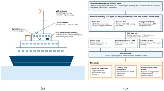
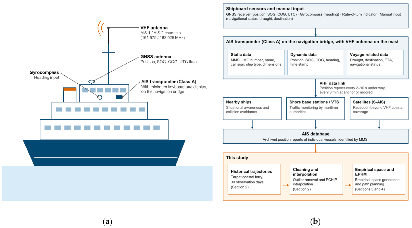
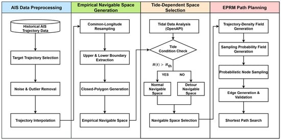
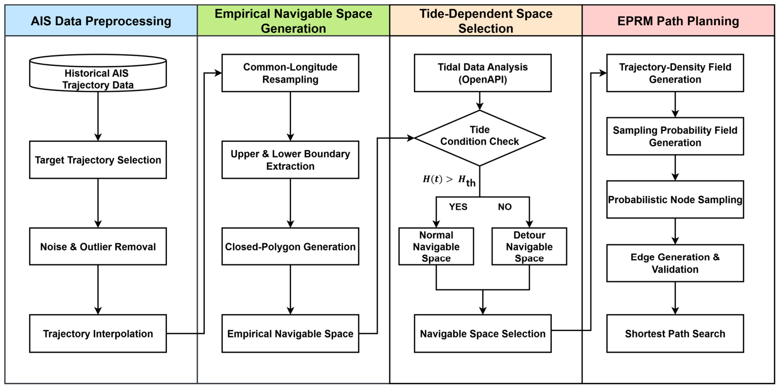
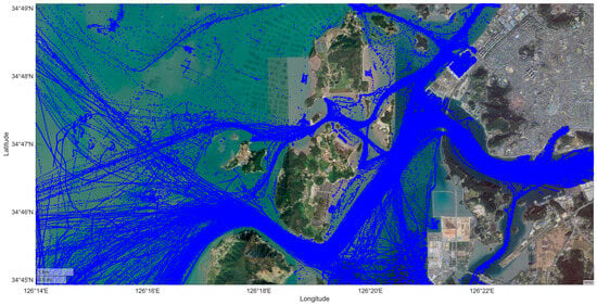
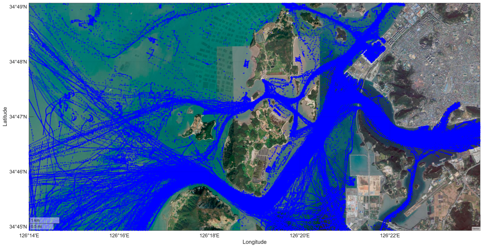
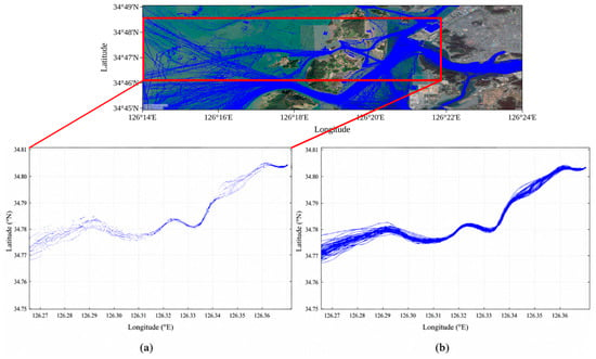
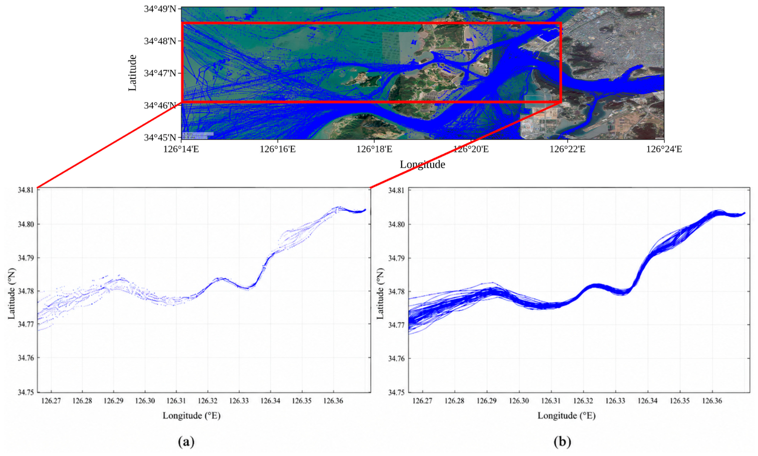
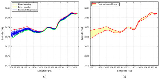
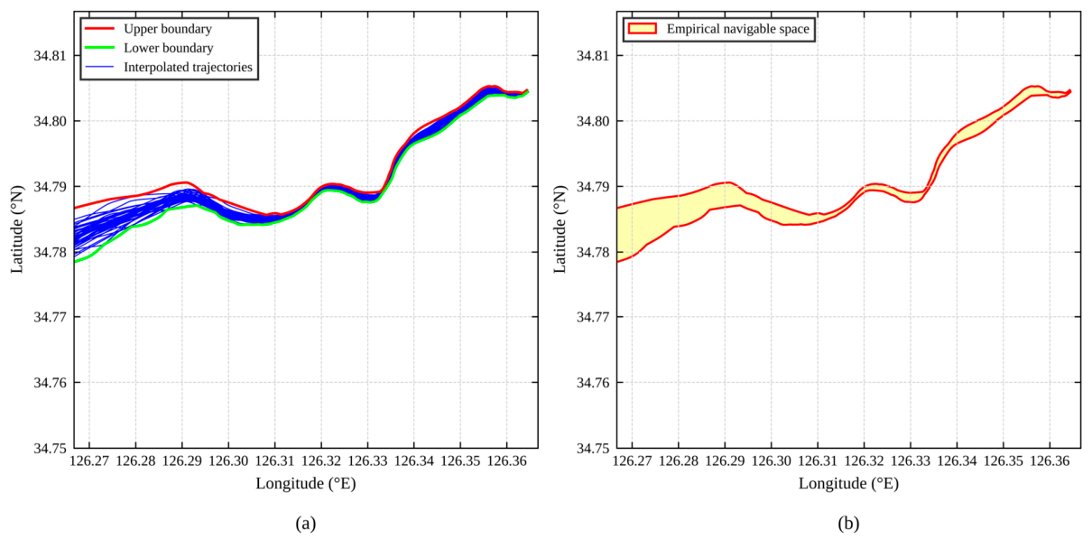
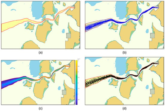
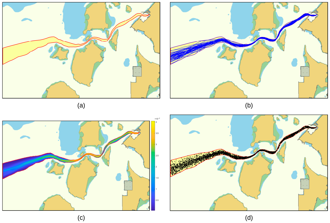
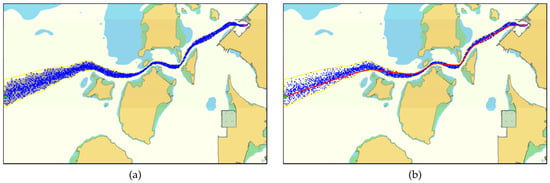
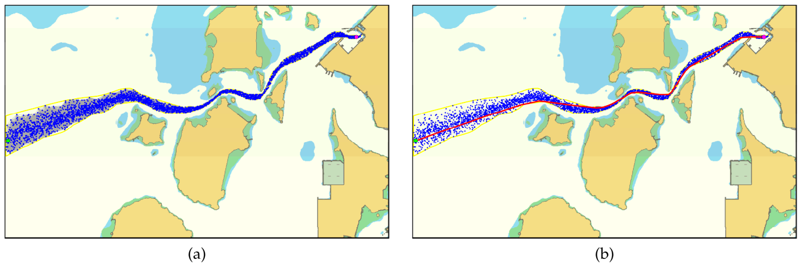
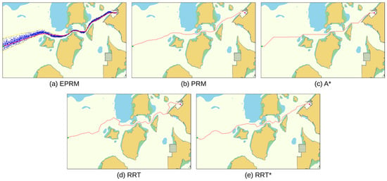
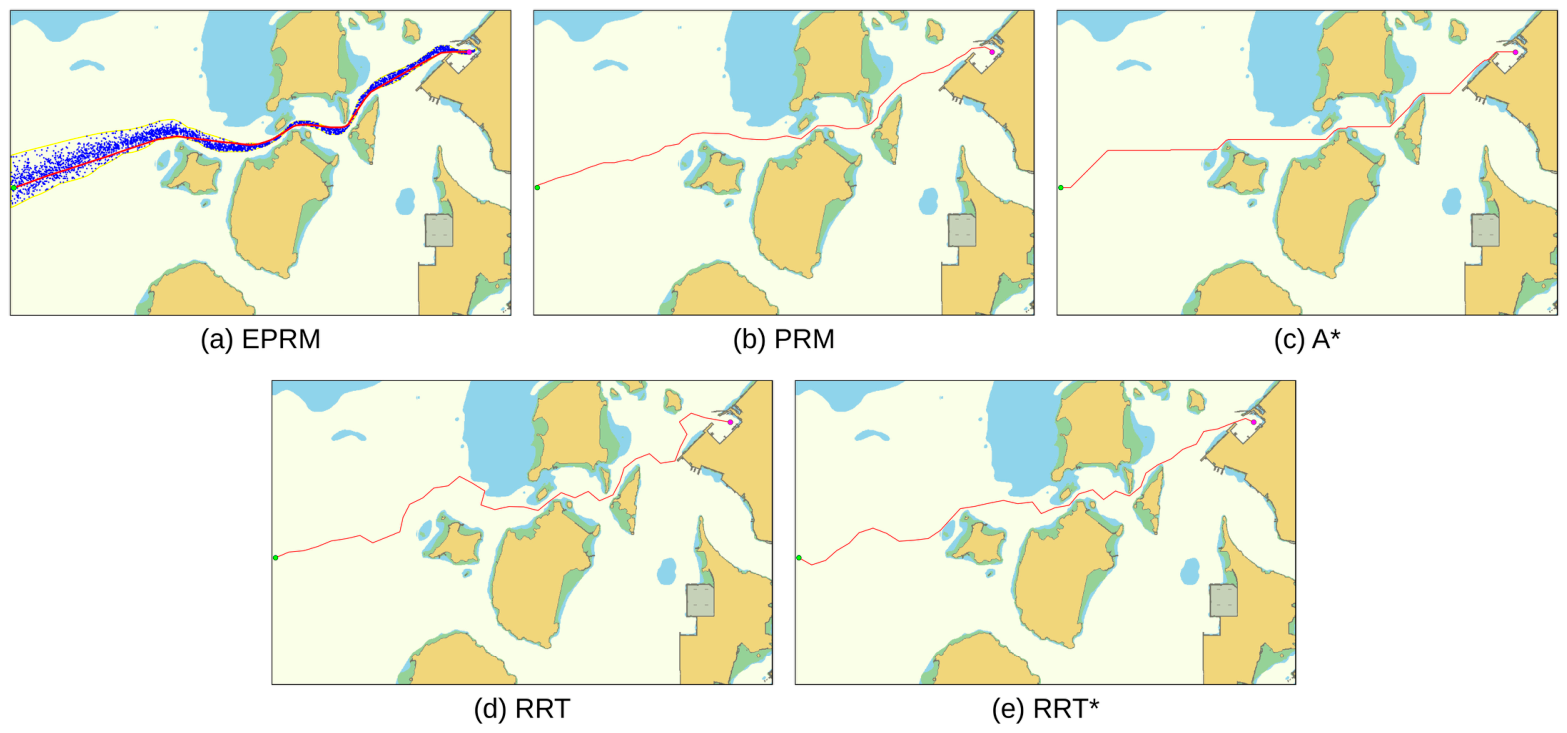
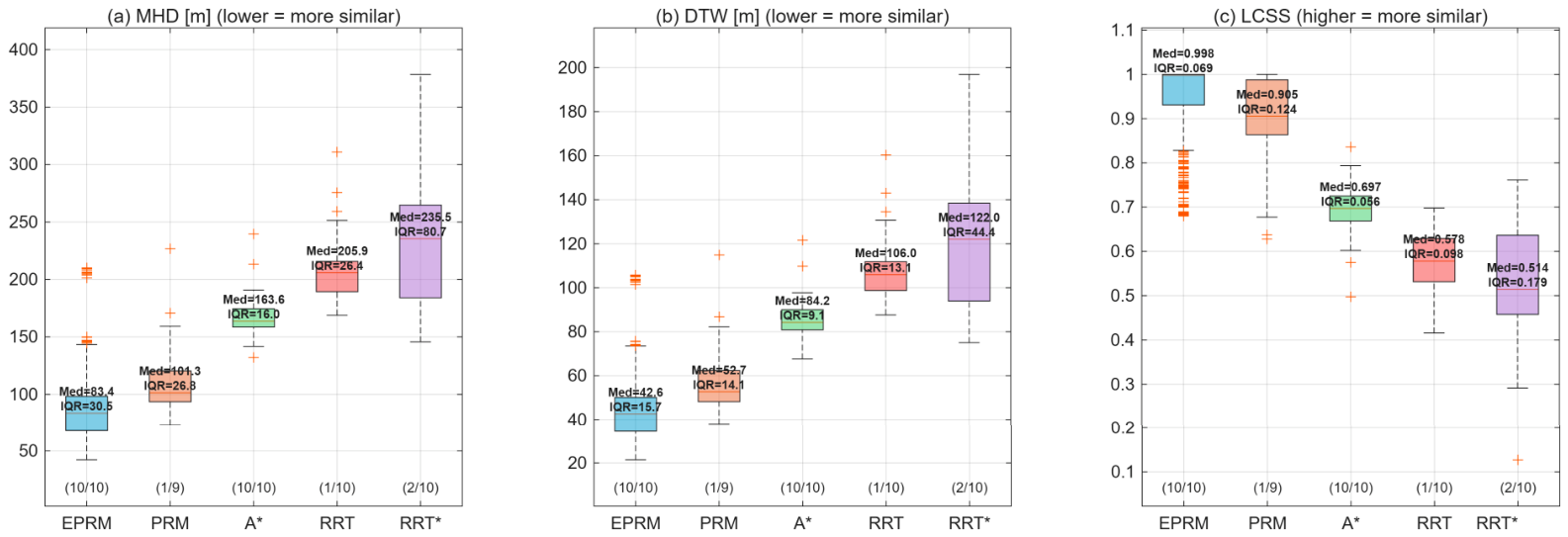
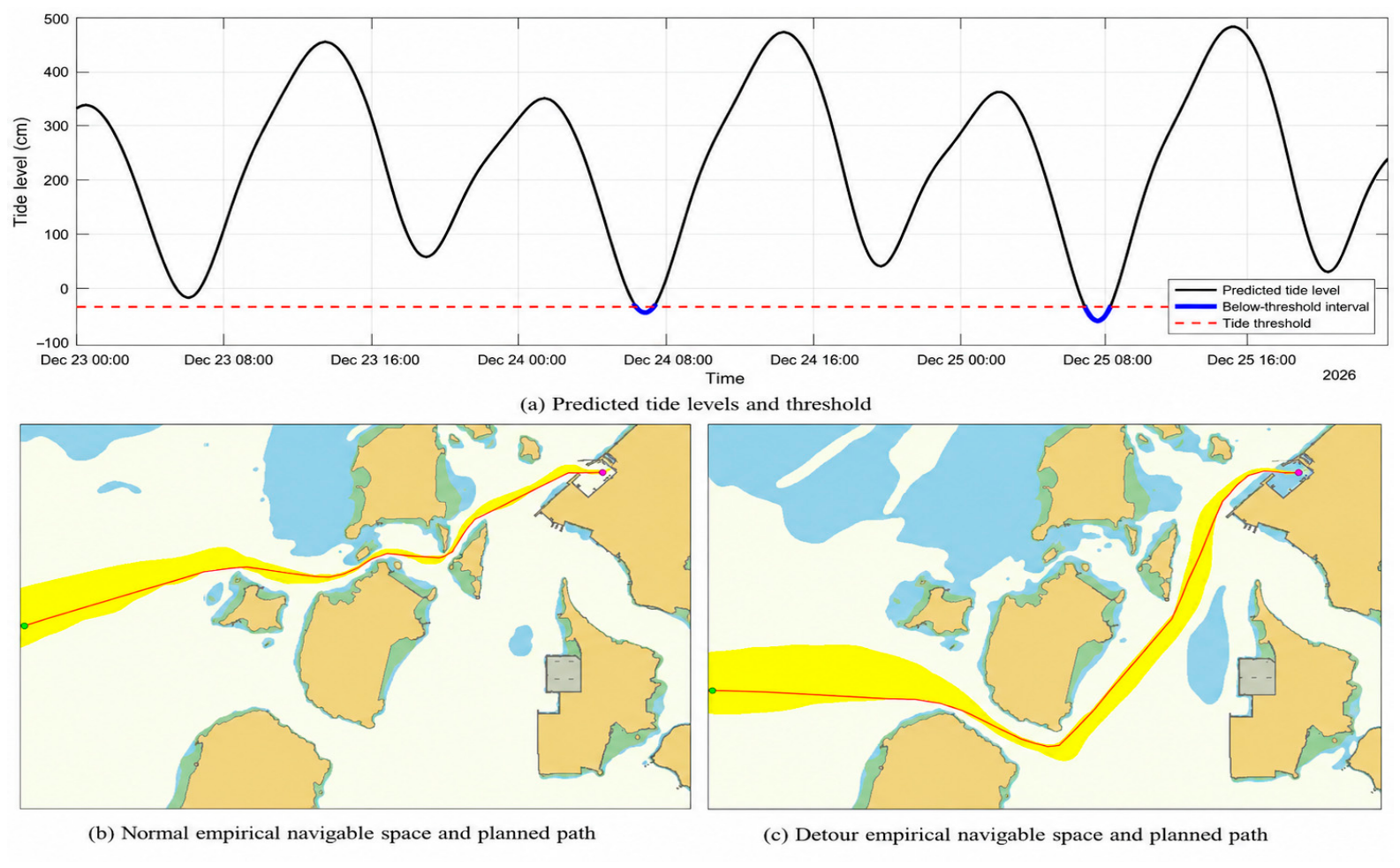

Disclaimer/Publisher’s Note: The statements, opinions and data contained in all publications are solely those of the individual author(s) and contributor(s) and not of MDPI and/or the editor(s). MDPI and/or the editor(s) disclaim responsibility for any injury to people or property resulting from any ideas, methods, instructions or products referred to in the content. |
© 2026 by the authors. Licensee MDPI, Basel, Switzerland. This article is an open access article distributed under the terms and conditions of the Creative Commons Attribution (CC BY) license.