


Abstract
Coastal protection structures are crucial for reducing wave impacts and protecting vulnerable shorelines and coastal ecosystems. The hydrodynamic performance of a Semicircular Breakwater with Cover (SBWC) under regular wave conditions was evaluated using physical flume experiments and computational fluid dynamics (CFD) modeling. A total of 216 regular-wave laboratory tests were conducted across four relative submergences (Rdh = d/h = 0.67, 1.00, 1.33, and 1.67), three wave steepness values (S1 = Hi/L= 0.02, 0.04, and 0.06), and 18 wave periods (T = 0.8–2.5 s), corresponding to relative breakwater widths (B/L = 0.17–1.22). CFD simulations were conducted in FLOW-3D using the Volume of Fluid (VOF) method and validated against physical flume measurements to assess the model’s ability to reproduce the hydrodynamic performance of the SBWC. The validated CFD model reproduced the measured transmission, reflection, and energy loss coefficients across all tested conditions, providing a basis for future investigations under other conditions within an appropriate range of applicability. Under emerged conditions (Rdh = 0.67), the SBWC functions primarily as a wave-reflecting structure, yielding low wave transmission (CT ≈ 0.07–0.37) and high reflection (CR ≈ 0.41–0.91). At the partially submerged condition (Rdh = 1.00), wave energy dissipation was maximized, with the energy loss coefficient (CL) reaching 0.93 due to wave breaking and turbulent shear across the SBWC. Non-linear multivariable empirical models incorporating second-order interaction terms were developed to predict CT, CR, and CL, with coefficients of determination of R2 = 0.84, 0.84 and 0.52, respectively (RMSE = 0.13, 0.10 and 0.12). Cubic polynomial models raised R2 to 0.91, 0.89 and 0.63. A comparison with the uncovered semicircular breakwater shows that the cover reduces wave transmission mainly when the still-water level is at the caisson crown. These findings quantify the hydrodynamic response of the SBWC and provide empirical equations for preliminary estimates of wave transmission, reflection and energy dissipation under regular waves, within the tested ranges.
1. Introduction
Coastal protection plays a vital role in safeguarding coastal communities, infrastructure, and maritime operations from wave action and shoreline erosion [1,2]. The design and hydraulic assessment of coastal protection structures depend on a reliable description of wave characteristics and wave–structure interaction [3]. Breakwaters are widely used as coastal defence structures to reduce wave height, attenuate wave energy, and modify the nearshore hydrodynamic environment [4,5]. They are broadly classified into rubble-mound, vertical and composite breakwaters, each exhibiting distinct hydraulic and structural characteristics [6]. In rubble-mound breakwaters, incident wave energy is dissipated by turbulence and friction within the porous armour, and the stability of their armour is governed by factors such as wave period, storm duration, structural permeability, and wave steepness [6,7]. Conversely, solid vertical breakwaters primarily reflect incoming wave energy and provide comparatively limited energy dissipation, and they must be designed to withstand severe wave impact loads [3,8]. The choice of breakwater type is thus a compromise between wave attenuation, structural stability, constructability and site-specific environmental constraints.
Nature-based solutions, such as mangrove forests, complement engineered coastal structures by attenuating waves and storm surges, stabilizing the shoreline and sequestering carbon in sheltered, muddy coastal areas [9,10]. Permeable breakwaters built from natural materials, such as bamboo wave screens and bamboo fences, have been used to reduce wave heights and promote sedimentation in front of mangrove belts [11,12]. However, despite restoration projects worldwide aimed at reversing losses caused by coastal development and other human activities [13,14], newly planted mangrove saplings suffer high mortality when exposed to strong hydrodynamic forces, substrate erosion and wave action [15,16,17]. Hybrid engineering structures that minimize the energy of incoming waves while maintaining nearshore hydrodynamic circulation can protect saplings during early establishment [2,18,19].
Conventional hard structures remain the most widely used form of coastal defence. Rubble-mound breakwaters depend on the stability of their armour layers to dissipate wave energy [7], whereas vertical and composite caisson breakwaters reflect much of the incident energy and require careful treatment of wave loads, scour and foundation stability [3,6]. Nature-based and hybrid solutions have been promoted as complements to hard structures because they combine wave attenuation with ecological benefits [20], but their performance is limited by the hydrodynamic loads that the natural element can tolerate. Semicircular breakwaters (SBWs) are hard, caisson-type structures whose curved profile is reported to reduce the horizontal wave load on the foundation and whose hollow interior reduces the concrete volume [2,5,19]. SBWs have been constructed in Japan and China and examined in emerged, free-surface and submerged configurations [2,21,22]. Reported limitations are that an emerged, solid SBW acts mainly as a wave reflector, while a submerged SBW transmits a large part of the incident wave energy [2,5,19]. Complete suppression of wave action is not required for applications such as mangrove protection on muddy coasts. In such settings, a small-scale submerged SBW that attenuates waves through partial reflection and breaking and transmits only part of the energy to the lee side, is adequate and has minimal visual impact on the coastal landscape. These limitations and functional requirements motivate geometric modifications to enhance energy dissipation without sacrificing structural stability, and they form the basis of the semicircular breakwater with cover (SBWC) investigated in this study.
The first prototype semicircular caisson breakwater was built at Miyazaki Port, Japan, in 1992–1993 and was designed to withstand severe storm waves [23,24,25]. Its performance encouraged the use of semicircular breakwaters at other ports in Asia, particularly in China. In 1997, a 527 m long semicircular breakwater was built to protect the southern area of Tianjin Port, China [26]. In 2000, the first phase of the Yangtze Estuary Deepwater Channel Improvement Project in Shanghai was completed, including an 18 km semicircular jetty [26]. More recently, SBWs have also been applied for shoreline protection on the Mekong Delta coast, Vietnam [25,27]. The caisson’s curved shape affects the interaction between incident waves and the breakwater, and the hollow design can reduce the structural mass and foundation loading compared with conventional solid caissons [2,5], and the semicircular geometry is also reported to offer good wave attenuation, inherent structural stability, cost efficiency and aesthetic appeal [19,21,22]. Based on their perforation arrangement, SBWs have been classified into four principal configurations: (a) impermeable SBW, (b) front-perforated, (c) rear-perforated, and (d) totally perforated structures [28,29], as shown in Figure 1.
Figure 1.
SBW types: (a) impermeable SBW, (b) front-perforated SBW, (c) rear-perforated SBW, (d) totally perforated SBW. Adapted from [2] (Al-Towayti et al., PLOS ONE, Public Library of Science, 2025), under the terms of the Creative Commons Attribution 4.0 International (CC BY 4.0) license.
2. Literature Review
Experimental, numerical, and field studies have investigated the hydraulic and structural response of SBWs under regular and random wave conditions [2,5,19,30,31,32]. Experimental studies have examined free-surface semicircular breakwaters under irregular waves, showing that porosity influences wave transmission, reflection, and energy dissipation, as well as the resulting wave forces [33]. Other investigations of semicircular breakwaters equipped with truncated wave screens demonstrated that the screen configuration affects CT and CL [34]. More recently, a pile-supported free-surface semicircular breakwater was examined under regular waves, showing that its hydrodynamic performance depends on wave conditions and structural geometry, with empirical relationships developed for the resulting hydrodynamic coefficients and wave forces [30]. Field monitoring of the Miyazaki Port SBW demonstrated that the curved caisson wall can reduce horizontal wave forces and consequently improve resistance to sliding during severe wave conditions [32]. Early experimental and numerical investigations quantified the wave pressures and forces acting on SBWs under emerged, alternately submerged and submerged conditions [28,35], while laboratory measurements showed that dynamic wave pressures on semicircular caissons vary with relative submergence ratio and wavelength [5,36]. In evaluating conventional wave-pressure formulations, the differences between Goda’s modified formulation and measured wave pressures on SBWs under different relative submergence ratios have been studied [3,28]. Subsequent experimental investigations demonstrated that rubble-foundation height, water depth, and caisson perforation ratio can substantially influence wave transformation around SBWs [37].
Other studies have examined the effects of porosity, submergence, wave steepness, and structural stability on SBW performance. Investigations of porous semicircular and cylindrical structures have shown that wave energy dissipation is influenced by incident wave height and chamber geometry [38]. For emerged breakwaters, the wave reflection increases with decreasing wave steepness and wave period [2,5,19]. For submerged configurations, wave reflection from vertical and semicircular breakwaters has been measured and empirical relationships for the reflection coefficient based on relative submergence have been developed [39]. Other studies investigated the sliding stability of semicircular breakwaters and reported that the required structural self-weight varies with wave steepness and water depth [40]. Collectively, these studies demonstrate that SBW performance is governed by the interaction between structural geometry, water depth, wave characteristics, and foundation conditions.
The application of SBWs has recently been extended to multifunctional and hybrid coastal protection systems. A VARANS model incorporating Biot’s partially dynamic seabed equations has been used to investigate porous submerged semicircular breakwaters combined with rear sloping breakwaters. The results indicated that the position of the porous breakwater relative to the incident wave field can influence wave energy dissipation and seabed response [41].
Later research integrated oscillating water columns (OWCs) with SBWs to examine the wave attenuation and wave energy conversion of such dual-function systems [42]. Numerical comparisons of submerged rectangular, sloping, and semicircular breakwaters using RANS k-ɛ turbulence modelling have further shown the influence of breakwater geometry on wave dissipation, local flow disturbance and near-bed turbulence [43]. These studies show the versatility of modified SBW configurations in multifunctional coastal engineering applications.
Numerical modelling has also advanced the study of nonlinear wave–structure interaction around complex coastal structures. Computational Fluid Dynamics (CFD) models based on the Volume of Fluid (VOF) method can capture free-surface deformation and the associated flow field around coastal structures [5]. FLOW-3D has been applied to a range of coastal engineering problems involving wave–structure interaction, including breakwaters and other complex hydraulic structures [5,44]. Previous studies have demonstrated that VOF-based FLOW-3D simulations can reproduce experimentally measured wave profiles, reflection characteristics, hydrodynamic pressures, and flow behaviour with reasonable agreement [5,45]. The combination of physical experiments and validated CFD modelling therefore provides a suitable framework for investigating modified breakwater geometries and their associated hydraulic and structural responses [5].
Despite these investigations, previous large-scale SBW studies have predominantly focused on conventional solid and perforated configurations, with modifications involving perforation arrangement, submergence, foundation geometry, or integration with other coastal and energy systems. The influence of incorporating a solid top cover across the upper portion of a small-scale semicircular caisson has not been systematically investigated. In particular, the effects of such a cover on wave transmission, reflection and energy dissipation have not been assessed. The proposed cover changes the wave-exposed geometry and local flow field around the caisson; its influence on the partition of wave energy therefore needs to be quantified. Furthermore, the internal space formed beneath the top cover may accommodate ballast material, providing a potential means of adjusting structural stability according to site-specific foundation and loading conditions.
Accordingly, this study introduces and investigates a modified small-scale semicircular breakwater with a top cover (SBWC) under regular wave conditions. The hydrodynamic performance of the SBWC, evaluated through the wave transmission coefficient (CT), reflection coefficient (CR), and energy loss coefficient (CL), is systematically assessed using physical flume experiments. A validated two-dimensional (x–z plane) CFD model (FLOW-3D) is then used to examine the wave–structure interaction and to verify the consistency of the measured coefficients. The influence of governing non-dimensional parameters including the relative submergence ratio (Rdh = d/h, where d is the still-water depth and h = 0.60 m is the characteristic caisson height), wave steepness (S1 = Hi/L, where Hi is the incident wave height and L is the local wavelength), and relative breakwater width (B/L, where B = 1.20 m is the base width of the breakwater) is analyzed across an extensive operational dataset (N = 216). Finally, second-order and cubic multiple polynomial regression (MPR) empirical relationships incorporating linear, quadratic, interaction and cubic terms are established to estimate the hydraulic performance of the proposed SBWC configuration within the tested ranges, for preliminary coastal engineering applications.
The structure of the paper is as follows. Section 2 reviews previous studies on SBWs and identifies the research gap. Section 3 outlines the physical experimental setup and wave measurement procedure. Section 4 presents the FLOW-3D numerical methodology and model validation. Section 5 describes the empirical regression approach. Section 6 presents and discusses the experimental, numerical, and empirical results. Section 6.4 quantifies the effect of the top cover by comparison with the uncovered SBW. Section 7 compares empirical models of increasing polynomial order and presents cubic equations. Section 8 summarizes the principal findings and conclusions.
3. Physical Experimental Methodology
3.1. Physical Wave Flume and SBWC Model Setup
Physical experiments were conducted at the Offshore Engineering Laboratory, Universiti Teknologi PETRONAS, in a wave tank measuring 20.0 m in length, 0.8 m in width, and 1.5 m in height. Regular waves were generated at the upstream boundary using a piston-type wavemaker that is equipped with an active wave absorption system capable of absorbing over 96.5% of reflected wave energy under target operating conditions [2,5]. To further minimize wave reflections from the downstream boundary, a passive beach absorber with a 1:10 slope was installed at the end of the tank.
The Semicircular Breakwater with Cover (SBWC) physical model was built at a Froude scale of 1:2.5 from reinforced concrete with a density of 2400 kg/m3 to suit the dimensions of the facility and to provide a stable model. As illustrated in Figure 2, the SBWC cross-section features an outer base radius R = 0.60 (yielding a total base width B = 1.20 m), a caisson body height of h = 0.60 m, an overall height including the 0.04 m top cover deck of ht = 0.64 m, and a longitudinal length of 0.80 m, spanning the full width of the wave tank. The self-weight of the concrete caisson was sufficient to prevent sliding and overturning under wave action. To prevent leakage and parasitic side flows during testing, the gaps between the model edges and the flume side walls were completely sealed using silicone sealant and cement. All internal joints and small gaps were thoroughly sealed with cement grout and silicone sealant to ensure structural impermeability, preventing water from entering or accumulating inside the breakwater caisson during overtopping events. The model therefore remained fixed throughout the tests, and the measurements represent the hydrodynamic response alone. The top cover extends across the crown section, adds to the resistance against wave-induced sliding and overturning, and is intended to modify the interaction between the incident wave crests and the structure and thereby to increase wave attenuation. Its configuration is shown in Figure 3.
Figure 2.
Isometric views of the SBWC components and their main dimensions: (a) top cover, (b) caisson body before assembly, and (c) assembled breakwater.
Figure 3.
Internal configuration of the SBWC model: (a) exploded view of the four internal units and partition walls; (b) assembled model with the top cover.
In the SBWC configuration, the open-top caisson body (Figure 2b) is capped at the crown by a solid cover deck (Figure 2a). This modification serves two distinct purposes: first, it forms an enclosed internal chamber that can hold ballast material to adapt structural weight to site-specific geotechnical and wave loading requirements; second, it alters the crest profile so that overtopping water streams across a continuous flat deck rather than plunging into an open cavity. The hydrodynamic changes induced by the capping of the crown, which alters the wave breaking, jet deflection and turbulence in the shear layer that controls wave transmission, reflection and energy loss, are quantified in Section 6.4. All internal seams and structural joints were fully sealed with cement grout and silicone sealant to prevent water from entering or accumulating inside the caisson during overtopping.
3.2. Regular Wave Test Conditions and Experimental Matrix
Experiments were performed under regular waves at four relative submergence ratios (Rdh = 0.67, 1.00, 1.33, and 1.67), corresponding to water depths of d = 0.40 m, 0.60 m, 0.80 m, and 1.00 m, respectively. As shown in the schematic cross-sections in Figure 4, these depths represent emerged, alternatively submerged, submerged, and deeply submerged operational states. Because the cover deck raises the overall crest of the SBWC to 0.64 m, the freeboard of the cover deck is +0.24, +0.04, −0.16 and −0.36 m at the four depths (d/ht = 0.63, 0.94, 1.25 and 1.56, where ht is the overall height including the cover). At Rdh = 1.00 the still-water level is therefore at the crown of the caisson body, while the cover deck lies 0.04 m above it and is alternately exposed and overtopped by each wave. Each test lasted 180 s, and a stable window of more than 20 consecutive steady-state waves was analysed. Table 1 summarizes the experimental parameters.
Figure 4.
Schematic cross-sections illustrating the wave-structure interaction setup for the SBWC model across the four tested relative submergence: (a) Rdh = 0.67, (b) Rdh = 1.00, (c) Rdh = 1.33, and (d) Rdh = 1.67.
Table 1.
Summary of physical experimental wave parameters and operational test conditions.
Because the SBWC spans the full flume width and all structural joints were hermetically sealed, no water entered the caisson chamber. Water carried over the crest during overtopping could return seaward only across the crest, which could induce a minor set-up of the mean water level on the lee side during emerged (Rdh = 0.67) and alternatively submerged (Rdh = 1.00) test conditions. To maintain rigorous experimental control, the still-water depth was verified prior to each test run, and the flume was allowed to settle completely between runs to ensure that every experiment started from the target depth (d).
Wave-depth regime. Using linear wave theory, the 18 wave periods give d/L = 0.08–0.40 for d = 0.40 m, 0.11–0.60 for d = 0.60 m, 0.13–0.80 for d = 0.80 m and 0.14–1.00 for d = 1.00 m (kd = 0.5–2.6, 0.7–3.8, 0.8–5.0 and 0.9–6.3, with k = 2π/L). All tests therefore lie in intermediate-depth (0.05 < d/L < 0.5) or deep-water (d/L ≥ 0.5) conditions; none is in the shallow-water regime. The long waves at the smaller depths are subject to stronger finite-depth and nonlinear effects than the short waves, whose orbital motion decays rapidly with depth so that they interact mainly with the upper part of the structure. For the fixed geometry tested, B/L, Hi/L and d/h determine d/L and the relative freeboard, and hence the wave period T.
3.3. Free-Surface Elevation Measurement and Wave Decomposition
As shown in Figure 5, surface elevation time series were recorded using six capacitance-type wave probes sampled at 50 Hz. All probes were calibrated before testing, achieving linear regression coefficients exceeding R2 = 0.9999 across all channels. Probes WP1, WP2, and WP3 were positioned upstream of the model to separate incident (Hi) and reflected (HR) wave components using the three-point least-squares method of Mansard and Funke [46]. Probes WP4, WP5, and WP6 were installed on the lee side to evaluate transmitted wave heights (HT).
Figure 5.
Plan and side views of the 20.0 m wave flume showing the wave maker, wave absorber, SBWC position, and wave probe locations (WP1–WP3 seaward and WP4–WP6 leeward) for Rdh = 0.67.
The seaward wave probes (WP1–WP3) were positioned according to standard wave-separation criteria, with X12 = L/10 and L/6 < X13 < L/3, where L is the local wavelength calculated using the linear wave dispersion relation (L = 0.985–6.964 m), to minimise errors in separating incident and reflected waves [47]. Specifically, X1 = 4.7 m represents the distance from the wavemaker paddle to the first wave probe (WP1) to allow full development of incident wave trains; X12 is the longitudinal spacing between WP1 and WP2, designed to resolve phase differentials without spatial aliasing; X13 is the longitudinal distance between WP1 and WP3, fulfilling the non-integer phase relationship required for the three-point wave separation method; and XR1 = 4.7 m denotes the offset distance from the first wave probe (WP1) to the front face of the breakwater model. The seaward array was positioned at an offset distance XR1/L = 0.67–4.77 (satisfying XR1 ≥ 0.5L across all test runs) upstream of the structure to avoid localized evanescent wave contamination and spatial disturbance from near-field wave reflections [46,48].
The spacing criteria follow Goda and Suzuki [48] and Mansard and Funke [46]. Placing the nearest gauge at a distance of the order of one wavelength or more from the structure is common practice for limiting the influence of evanescent modes generated at the structure [46,48]. WP2 and WP3 were repositioned for each wave condition according to the corresponding wavelength (L = 0.985–6.964 m) so that X12 = L/10 and L/6 < X13 < L/3. WP1 was kept at a fixed distance of XR1 = 4.7 m from the front face of the structure (XR1/L = 0.67–4.77); for the longest waves this is less than one wavelength. The gauge configuration affects the uncertainty of the incident–reflected wave separation [47].
3.4. Hydrodynamic Performance Assessment
The hydraulic efficiency and wave attenuation capability of the Semicircular Breakwater with Cover (SBWC) are evaluated using non-dimensional hydrodynamic performance coefficients: the transmission, reflection and energy loss coefficients.
The transmission coefficient (CT) quantifies the proportion of wave height transmitted past the structure to the lee side:
where HT represents the transmitted wave height, measured by the leeward probe array (WP4–WP6), and Hi is the incident wave height resolved from the seaward probe array (WP1–WP3) using the Mansard and Funke wave decomposition method [46].
The reflection coefficient (CR) represents the fraction of the incident wave height reflected seaward from the breakwater front face:
where HR is the reflected wave height. Applying conservation of wave energy flux across the surrounding fluid domain yields the energy balance relation:
Rearranging Equation (3) yields the wave energy dissipation coefficient (CL), representing wave energy loss driven by crest overtopping, surface wave breaking, turbulent friction across the SBWC, and vortex shedding near the structural edges:
4. Numerical Methodology and Computational Approach
4.1. Numerical Rationale and Validation Setup
Two-dimensional (x–z plane) computational fluid dynamics (CFD) simulations were performed using FLOW-3D to complement the physical flume experiments and evaluate the model’s ability to reproduce the measured hydrodynamic coefficients (CT, CR and CL). The computational settings, including grid resolution, time-step stability criteria (CFL ≤ 1.0), and wave-absorber sponge-layer parameters, were established to ensure numerical stability and appropriate wave propagation and absorption.
The model was evaluated against the experimental results across the investigated ranges of relative submergence ratio (Rdh = 0.67–1.67), wave steepness (S1 = 0.02–0.06), and relative breakwater width (B/L = 0.17–1.22). Numerical wave probes were positioned at the same locations as the physical wave gauges (WP1–WP6). The simulated hydrodynamic coefficients were compared with the corresponding experimental values using the mean squared error (MSE), root mean square error (RMSE), mean absolute deviation (MAD), mean absolute percentage error (MAPE), and coefficient of determination (R2). The results quantify the agreement for each submergence ratio and wave steepness range. The CFD model thus provides an independent check on the laboratory results within the tested range.
4.2. Description of Computational Modelling Approach
The numerical simulations were performed in FLOW-3D. The SBWC model was generated in SolidWorks (version 2023; Dassault Systèmes, Vélizy-Villacoublay, France) and imported into the solver in Stereolithography (.stl) format. Computations were performed in a numerical wave tank measuring 20.0 m long, 1.5 m high, and 0.8 m wide.
A multi-block nested mesh was adopted to limit the computational cost while resolving the flow in the vicinity of the caisson. The background grid had cell dimensions of Δx = Δz = 0.04 m to resolve wave propagation throughout the flume domain. A locally refined nested grid with cell dimensions of Δx = Δz = 0.02 m was applied around the structure to better capture wave–structure interactions and local flow variations [5]. The SBWC was located near the middle of the tank, leaving sufficient length upstream for wave development and downstream for wave decay.
Free-surface kinematics and non-linear wave deformation around the breakwater cross-section were resolved using the Volume of Fluid (VOF) method [5]. Four relative submergence ratios (Rdh = 0.67, 1.00, 1.33, and 1.67) were evaluated to model the target operational states. Six numerical wave probes recorded surface elevation time-series along the channel. Upstream probes WP1, WP2, and WP3 recorded composite wave fields for incident and reflected wave decomposition via the three-point least-squares technique of Mansard and Funke method [46], while leeward probes WP4, WP5, and WP6 measured transmitted wave heights.
As illustrated in the computational domain schematic (Figure 6), the boundary conditions were specified to replicate the laboratory setup. At the upstream inlet (Xmin), regular incident waves were prescribed using FLOW-3D’s wave boundary condition based on linear wave theory. Target wave heights and periods from each laboratory test defined the input wave signals, and the resulting incident wave heights recorded at numerical probes WP1–WP3 were verified against physical flume measurements. At the downstream boundary (Xmax), an active absorption condition combined with a 2.0 m sponge layer was implemented to damp transmitted waves and minimize artificial reflections, taking the place of the 1:10 passive beach installed in the flume. The upper boundary (Zmax) was defined as an atmospheric-pressure boundary, while the tank bed (Zmin) was modelled as a smooth, no-slip wall representing the concrete laboratory floor. Bed friction was accounted for through the no-slip condition and the standard wall-function treatment in the turbulence model. Symmetry boundary conditions were applied to the lateral boundaries (Ymin and Ymax). As the SBWC extended across the full width of the flume, the flow field was assumed to be essentially two-dimensional in the x–z plane, consistent with the two-dimensional numerical formulation described in Section 4.3. Finally, numerical wave probes (WP1–WP6) were placed at the same locations as the physical wave gauges to extract the wave parameters and enable direct comparison between the numerical predictions and experimental measurements.
Figure 6.
Computational domain setup in FLOW-3D, detailing boundary conditions, mesh refinement zones, SBWC model placement, and wave probe locations (WP1–WP6).
4.3. Governing Equations of Computational Model
Fluid flow within the x-z plane is governed by the two-dimensional incompressible Reynolds-Averaged Navier–Stokes (RANS) equations, along with the continuity equation [5]. Incorporating fluid density, volume fractions, and mass source terms, the general continuity equation is expressed as:
Assuming an incompressible fluid = constant), Equation (5) simplifies to:
The horizontal (x) and vertical (z) Cartesian momentum equations are defined as:
where u and w are the fluid velocity components in the x and z directions, respectively; t is time; Ax and Az denote the fractional area fractions open to flow; VF is the open volume fraction, ρ is fluid density, P is pressure, RDIF is turbulent diffusion, and RSOR represents mass source inputs, (Gx, Gz), is body accelerations, (fx, fz), is viscous accelerations, (bx, bz) account for hydraulic head losses across solid obstacles, and (us, ωs) are mass injection velocity components.
4.4. Free-Surface Modelling Using the Volume of Fluid (VOF) Method
Free-surface motion was tracked using the Volume of Fluid (VOF) formulation, which computes local fluid volume fractions within each computational cell while enforcing interface boundary conditions. The spatial distribution of water is defined by a scalar fluid fraction function F, where empty cells (F = 0) represent the gas phase, submerged cells F = 1 represent the fluid phase, and interface cells fall within 0 < F < 1 (Figure 7). Neglecting air-phase calculations in empty cells optimizes computational efficiency without altering surface wave kinematics. Two-dimensional advection of F is governed by:
where vF is the fluid diffusion coefficient and FSOR represents volume source terms.
Figure 7.
Cross-sectional grid schematic of the Semicircular Breakwater with Cover (SBWC) model showing Volume of Fluid (VOF) cell tracking configurations (F = 0, 0 < F < 1, F = 1).
4.5. Turbulence Closure Model
Turbulence was modelled using the standard two-equation k-ɛ model [49], which calculates transport equations for turbulent kinetic energy (k) and its dissipation rate (ɛ). It should be noted that standard two-equation RANS closures are known to potentially over-predict turbulence production under surface gravity waves unless specific stabilization or modified closures are applied [50].
where Pk is shear production, Gk is buoyancy production, represents eddy viscosity, and are the turbulent Prandtl numbers for k and , respectively; and standard closure coefficients were applied ( = 0.09, = 1.44, = 1.92, = 1.0, = 1.3). No-slip wall conditions were applied along the solid SBWC boundary, with the wall turbulence mixing length determined dynamically.
The model was validated through direct comparison of the simulated and measured values of CT, CR, and CL across the tested operational spectrum. The standard k–ε turbulence model was selected because it efficiently resolves free-surface deformation and far-field wave propagation while maintaining numerical stability during complex overtopping events over the cover deck. Identical standard closure coefficients were used in all simulations.
4.6. Mesh Sensitivity Analysis and Grid Independence
Mesh convergence was assessed using different levels of mesh resolution, ranging from coarse background grids to fine local grids. The mean flow velocity (u) and corresponding Froude number (, where g = 9.81 m/s2 is gravitational acceleration and d is the water depth) for each tested mesh configuration are presented in Table 2.
Table 2.
Flow velocity and Froude number sensitivity results obtained using different cell sizes tested in FLOW-3D.
The mean velocity (0.039 m/s) and Froude number (0.073) showed negligible changes when the local structural grid was refined from Δx = 0.02 m to 0.01 m. A 0.04 m background mesh combined with a 0.02 m local mesh around the structure was therefore adopted, offering adequate resolution at a reduced computational cost.
The Froude numbers reported in Table 2 represent time-averaged local flow velocities recorded at a single monitoring point during the calibration run and serve only as an indicator of mesh convergence; they do not characterise the wave kinematics of the test programme. Across the 216 test cases, the estimated orbital velocity ranges from 0.08 to 0.68 m/s, corresponding to (Frw) values of approximately 0.03–0.22. The wave-induced flow is therefore subcritical. However, localized high velocities, potentially including supercritical flow, may occur in thin overtopping jets above the cover deck. Although the VOF method captures the free-surface evolution associated with such flows, their accurate resolution depends on the computational mesh. The numerical model was validated within the range of experimentally investigated conditions.
4.7. Dynamic Adaptive Time-Stepping and Stability Criteria
To maintain numerical stability in the transient wave calculations, time steps were dynamically adjusted based on the Courant-Friedrichs-Lewy (CFL) criterion:
where = 0.02 m represents the minimum local spatial cell size, is local flow velocity, g = 9.81 m/s2, d is the water depth, VF denotes the fractional volume available for flow, and Ai represents the fractional area available for flow. The Courant limit was set at CFL ≤ 1.0 with a safety factor of 0.85, which limits the time-step bounds between ∆tmin = 0.0008 s and ∆tmax = 0.0160 s.
In a typical run, the time step passed through three phases over the 3.0 min (180 s) simulation period. As shown in Figure 8, prior to wave arrival (t < 0.2 min), time steps remained near the upper bound 0.0160 s). As waves interacted with the caisson crest (0.2 min t 1.25 min), localized velocity increases caused time steps to adjust dynamically between 0.002 s and 0.007 s to satisfy the CFL limit. Once wave overtopping and turbulence fully developed (t 1.25 min), time steps stabilized around an average value of 0.0024 s.
Figure 8.
Time-step evolution over a 3.0 min simulation duration (18,000 sampling points) for the SBWC model.
4.8. Statistical Validation and Error Analysis
To quantify the predictive accuracy and validate the agreement between experimental physical tank observations (Ai) and numerical or empirical predictions (Mi) across n test conditions, a comprehensive suite of statistical metrics is evaluated. The coefficient of determination (R2) assesses the proportion of variance in the experimental data explained by the model:
where denotes the arithmetic mean of the measured experimental values. To penalize larger localized discrepancies and evaluate the average absolute deviation magnitude, the Mean Square Error (MSE) and Root Mean Square Error (RMSE) are expressed as:
Furthermore, the Mean Absolute Deviation (MAD) measures the average absolute magnitude of the prediction errors, while the Mean Absolute Percentage Error (MAPE) quantifies the relative discrepancy in percentage terms:
In the following sections, R2 values close to 1.0 together with low RMSE, MAD and MAPE values are taken to indicate good agreement across the tested ranges of wave steepness (S1) and relative submergence ratio (Rdh).
5. Empirical Regression Modeling Methodology
Non-linear predictive relationships for CT, CR, and CL were derived through multivariable regression in IBM SPSS Statistics 27 (IBM Corp., Armonk, NY, USA) (second-order models) and Design-Expert 13 (higher-order models, Section 7). The model evaluates the dependent hydraulic coefficients (CT, CR, CL) against the non-dimensional governing parameters .
Multiple Linear Regression (MLR) was evaluated initially:
where Y represents the dependent hydraulic performance coefficients CT, CR, CL, is the intercept, are partial regression coefficients, and ɛ is the residual error.
Initial diagnostic evaluation confirmed that single-variable linear and power-law formulations were insufficient to model the non-linear hydraulic transitions across the evaluated submergence range (Rdh = 0.67–1.67). Consequently, a second-order polynomial model with cross-variable interaction terms was adopted. This quadratic interaction approach accounts for non-linear coupling among relative breakwater width ( = B/L), wave steepness ( = S1), and relative submergence ( = Rdh) during crest overtopping, jet deflection, and vortex generation across the SBWC. The unified quadratic interaction model is expressed as:
where a1 through a9 denote partial regression coefficients, and a10 is the intercept term. Predictive performance was assessed using MSE, RMSE, MAD, MAPE, and R2.
The second-order polynomial was initially selected as a relatively simple empirical formulation capable of capturing the nonlinear relationships between CT, CR, and CL and B/L, including the changes in trends observed between emerged and submerged conditions. Polynomial-based empirical approaches have been used in previous studies to describe and predict the hydrodynamic performance of semicircular breakwaters [2,30,33]. Higher-order polynomial formulations were also evaluated, and their comparative performance is discussed in Section 7.
Wave period (T) is represented in the model through the wavelength, L (T, d), which defines both B/L and S1. For a fixed structure geometry where B and h are constant, the experimental inputs (T, Hi, d) map directly to the non-dimensional parameters B/L, S1, and Rdh. For a given depth, B/L is a one-to-one function of T, so the effect of wave period on overtopping and transmission is represented through B/L (and, for a given steepness, through the wave height). A polynomial in these ratios cannot reproduce every functional form exactly, which may introduce a small bias in overtopping-dominated conditions. Across the tested wave periods (0.8 s < T < 2.5 s), B/L varied smoothly from 0.17 to 1.22, providing a one-to-one correspondence at each relative submergence level.
Model calibration was performed using the valid runs of the 216 tests. Predictive capability was assessed by leave-one-out cross-validation (PRESS) in Design-Expert 13 (Section 7). All proposed equations remain purely empirical and must be restricted to the validated ranges of Rdh, B/L, and S1.
6. Results and Discussion
On interaction with the Semicircular Breakwater with Cover (SBWC), the incident wave energy is partitioned into reflected, transmitted and dissipated components. The relative submergence ratio (Rdh) and relative breakwater width (B/L) are the main governing parameters controlling the distribution of energy among these components, while wave steepness (S1) has a secondary influence. The solid top cover changes the near-field flow kinematics under emerged and submerged conditions. Under emerged conditions, it acts as a wave-deflecting ledge that blocks advancing wave crests, causing wave breaking and overtopping. Under submerged conditions, it forms a turbulent shear layer that disrupts particle orbital motion while allowing deeper velocity fields to pass downstream with limited interference. These processes are examined in the following sections on the basis of the flume measurements, FLOW-3D simulations and empirical models.
6.1. Wave Transmission Coefficient (CT)
Wave transmission past the SBWC was evaluated experimentally and numerically in terms of the transmission coefficient (CT), calculated as the ratio of transmitted wave height (HT) to the incident wave height (Hi). A lower CT value indicates that the SBWC is more effective in attenuating wave energy.
6.1.1. Experimental Wave Transmission Coefficient
The experimental tests were conducted using regular waves at four relative submergence ratios (Rdh = 0.67, 1.00, 1.33, and 1.67). Figure 9 presents the variation in the CT with B/L for different wave steepness ranges.
Figure 9.
Experimental wave transmission coefficient (CT) against relative breakwater width (B/L) at relative submergence ratio (Rdh) of: (a) emerged (Rdh = 0.67); (b) alternatively submerged (Rdh = 1.00); (c) submerged (Rdh = 1.33); and (d) deeply submerged (Rdh = 1.67).
For the emerged condition (Rdh = 0.67), CT remains relatively low, ranging from approximately 0.07 to 0.37 (Figure 9a). A clear reduction in CT is observed as B/L increases, with values approaching 0.07 for B/L > 0.8. In this condition, the caisson and cover extend above the water surface and directly intercept the incoming wave crests. A large proportion of the incident energy is consequently reflected or dissipated by breaking and local turbulence, and only a limited fraction is transmitted by overtopping. The increase in B/L corresponds to a reduction in relative wavelength, resulting in stronger interaction between the incoming waves and the SBWC. At lower B/L, where the waves are relatively longer, a greater portion of the wave motion can pass over the structure, giving higher CT values.
A similar decreasing trend is observed for Rdh = 1.00 (Figure 9b). Here, CT ranges from approximately 0.07 to 0.61. The higher values occur mainly at lower B/L, where the longer waves interact with the structure over a larger vertical portion of the water column. As B/L increases, the interaction between the wave crests and the top cover becomes stronger, accompanied by local breaking, turbulent flow, and flow deflection around the cover. Consequently, the transmitted wave height decreases, with CT falling below approximately 0.20 at the higher B/L values.
A markedly different behaviour is observed once the SBWC is fully submerged. At Rdh = 1.33, the measured CT values range from approximately 0.55 to 0.97 (Figure 9c), while values between 0.59 and 0.97 are obtained at Rdh = 1.67 (Figure 9d). In both cases, CT generally increases with B/L, which is opposite to the trend observed for the emerged and partially submerged conditions. This behaviour is attributable to the vertical distribution of the wave-induced orbital motion. For shorter waves, corresponding to higher B/L, the orbital velocity decreases more rapidly with depth. The flow motion near the submerged portion of the SBWC is therefore weaker, allowing a larger proportion of the incident wave to pass over the structure with limited disturbance. Longer waves, represented by lower B/L, produce orbital motions that extend farther into the water column and interact more strongly with the submerged caisson, resulting in greater attenuation.
The effect of S1 is comparatively smaller than that of Rdh and B/L. Under emerged and partially submerged conditions, the steeper waves (0.04 < S1 ≤ 0.06) generally produce higher CT values. For a given B/L, steeper waves have larger crest heights relative to the freeboard of the cover deck and therefore overtop the structure more readily, so that a larger volume of water is carried to the lee side despite the additional breaking. Under fully submerged conditions, variations in S1 have a less pronounced effect on CT, as the wave-induced flow field interacts less strongly with the submerged structure.
6.1.2. Computational Wave Transmission Coefficient
The CFD simulations were carried out in FLOW-3D with the Volume of Fluid (VOF) free surface tracking and the standard k-ɛ turbulence closure model. Figure 10 compares experimental (Exp) and computational (Comp) CT against B/L for different Rdh and wave steepness ranges. The computational model is able to represent the wave transformation trends in the overall field, the near field overtopping kinematics, and the wave attenuation in the leeward direction for all tested operational states.
Figure 10.
Comparison of experimental (Exp) and computational (Comp) wave transmission coefficients (CT) for the SBWC at different B/L, Rdh and S1.
The numerical predictions were compared with the flume measurements using five statistical indicators for all operational states (Table 3): MSE, RMSE, MAD, MAPE, and R2.
Table 3.
Statistical performance metrics for measured and computational wave transmission coefficients (CT) across Rdh) and S1.
As shown in the statistical results in Table 3, the submerged configuration (Rdh = 1.33 and 1.67) exhibits very high predictive accuracy (R2 = 0.97–0.98) for the entire range of wave steepness. The low residual errors in Table 3, with MSE values of 0.00, RMSE values between 0.04 and 0.05 and MAD values of 0.03, indicate that the VOF interface tracking algorithm accurately resolves sub-surface fluid kinematics, wave dispersion, and the interaction between deeper water particle orbits and the caisson crown deck.
For the emerged (Rdh = 0.67) and alternatively submerged (Rdh = 1.00) states, Table 3 indicates that the computational model maintains strong correlation with physical observations, achieving R2 values ranging from 0.76 to 0.93. The minor reduction in R2 under low steepness (S1 ≤ 0.02) for Rdh = 0.67 (R2 = 0.84) and high steepness (0.04 < S1 ≤ 0.06) for Rdh = 0.67 (R2 = 0.76) and Rdh = 1.00 (R2 = 0.84) is attributable to complex non-linear air-water entrainment, localized wave slamming, and violent jet breaking across the top cover deck. In the physical flume, highly aerated overtopping flows generate three-dimensional air entrainment and turbulent spray that a single-phase VOF continuum formulation approximates with slight energy smoothing. Across all operational conditions in Table 3, MAPE remains low and maximum RMSE does not exceed 0.13, confirming that the FLOW-3D numerical setup accurately predicts wave attenuation past the SBWC.
6.1.3. Empirical Wave Transmission Coefficient
To provide a direct formulation for wave transmission past the SBWC without requiring CFD computations, an empirical model was established using multivariable regression. The (CT) is expressed as a function of three dimensionless parameters: ( = B/L), ( = S1), and ( = Rdh):
First-order linear and power-law relationships were insufficient to capture the hydrodynamic transitions across the emerged, alternatively submerged, and submerged regimes. Consequently, a second-order polynomial model with cross-variable interaction terms was adopted to account for coupling between wavelength, steepness, and water depth during crest overtopping and wave attenuation:
where a1 through a9 are partial regression coefficients and a10 is the intercept constant. The coefficients in Equation (22) were calibrated in IBM SPSS and are summarized in Table 4.
Table 4.
Empirical model parameters and regression coefficients for the wave transmission coefficient (CT) prediction model.
To prevent extrapolation errors, application of Equation (22) is restricted to the non-dimensional parameter range evaluated during physical testing:
Figure 11 compares the predicted (CT) and measured (CT) transmission coefficients for the regular wave conditions tested. The data points cluster along the 1:1 good agreement line (y = x), showing that the predictions follow the measured values over the full tested range of CT (0.06–0.97). The scatter about the 1:1 line is moderate (RMSE = 0.13); the cubic model presented in Section 7 reduces the RMSE to 0.09.
Figure 11.
Comparison between empirical non-linear model predictions and experimental measurements of the wave transmission coefficient (CT) for the SBWC relative to the 1:1 ideal agreement line (y = x).
Statistical performance metrics evaluated across the full experimental dataset confirm moderate overall predictive accuracy (Table 5).
Table 5.
Statistical performance metrics comparing experimental and empirical wave transmission coefficients (CT) for the SBWC.
As shown in Table 5, the non-linear interaction model yields a coefficient of determination of (R2 = 0.84) with residual errors (RMSE = 0.13, MAD = 0.10).
To confirm the performance of Equation (22) under specific water depth and steepness conditions, Figure 12 compares experimental CT (Exp), and empirical CT (Emp) plotted against B/L.
Figure 12.
Comparison of experimental (Exp) and empirical (Emp) wave transmission coefficients (CT) for the SBWC) at different B/L, Rdh and S1.
The empirical curves in Figure 12 closely follow the measured decay of CT in emerged (Rdh = 0.67) and alternatively submerged (Rdh = 1.00) states, as well as the higher transmission typical of deeply submerged runs (Rdh = 1.33 and 1.67). When quadratic and interaction terms are added to Equation (22), it reproduces the general transition from full wave obstruction to the overtopping of the crown and the passage of waves unhindered over the submerged deck and provides a direct formula for preliminary hydraulic design.
6.2. Wave Reflection Coefficient (CR)
Wave reflection governs the proportion of incident energy returned towards the wave generator rather than transmitted past or dissipated by the structure. The magnitude of reflection is mainly influenced by Rdh, S1, and the geometry of the curved seaward-facing caisson. Under emerged conditions, the exposed seaward surface directly intercepts the incoming wave and reflects a substantial portion of the incident energy back toward the wave generator. As the structure becomes submerged, wave crests can pass over the cover with less direct interaction with the seaward surface, resulting in lower CR values. These reflection characteristics are examined below using physical flume measurements, CFD simulations, and empirical formulations.
6.2.1. Experimental Wave Reflection Coefficient
The reflective response of the SBWC determines the amount of incident wave energy returned seaward rather than transmitted or dissipated around the structure. The incident (Hi) and reflected (HR) wave components were separated using the three-point least-squares method of Mansard and Funke [46], and the reflection coefficient was calculated as CR = HR/Hi. Figure 13 presents the variation in CR for different Rdh and wave steepness ranges.
Figure 13.
Experimental wave reflection coefficient (CR) against relative breakwater width (B/L) at relative submergence ratios (Rdh) of: (a) emerged (Rdh = 0.67); (b) alternatively submerged (Rdh = 1.00); (c) submerged (Rdh = 1.33); and (d) deeply submerged (Rdh = 1.67).
Under emerged conditions (Rdh = 0.67; Figure 13a), the SBWC behaves primarily as a wave reflector, with CR ranging from 0.41 to 0.91. The impermeable curved seaward caisson and top cover form a continuous barrier that intercepts the incident waves and returns a large part of their energy towards the wave generator. The highest reflection is observed for low-steepness waves (S1 ≤ 0.02), for which CR reaches approximately 0.61–0.91. At these lower steepness values, less energy is lost through wave breaking before the incident wave reaches the structure, allowing a larger portion of the wave energy to be reflected.
When the water surface is approximately level with the caisson crown (Rdh = 1.00; Figure 13b), the overall reflection decreases, with CR ranging from 0.16 to 0.72. The decrease in CR is particularly pronounced as B/L increases to approximately 0.5, after which the reflection coefficient approaches a relatively low range of about 0.16–0.25. At lower B/L values (B/L < 0.4), the longer waves interact more strongly with the caisson profile, resulting in greater reflection. As B/L increases, shorter waves interact more directly with the cover and are more readily dissipated through breaking and turbulent flow, reducing the amount of energy returned seaward.
For the submerged (Rdh = 1.33) and deeply submerged (Rdh = 1.67) conditions (Figure 13c,d), reflection is considerably lower, with CR ranging from 0.03 to 0.55. Values of CR greater than 0.30 occur mainly for longer waves (B/L < 0.3). At higher B/L values, CR generally falls below 0.20. The reduction in reflection is consistent with the rapid decay of wave-induced orbital motion with depth, which weakens the interaction between shorter waves and the submerged portion of the SBWC. Most of the incident motion therefore passes over the submerged structure with little reflection.
Wave steepness (S1) also affects the reflection response, although its influence is less pronounced than those of Rdh and B/L. Under emerged conditions, the lower-steepness waves generally produce higher CR values because a larger proportion of the incident energy reaches the seaward face without being dissipated by breaking. As wave steepness increases, wave breaking and turbulent dissipation become more pronounced around the SBWC, reducing the energy available for reflection. This effect becomes less evident under submerged conditions, where the wave-induced orbital motion is already strongly reduced with depth and the influence of wave steepness on CR is comparatively limited.
6.2.2. Computational Wave Reflection Coefficient
The numerical setup for wave reflection was validated by comparing FLOW-3D simulations with physical flume measurements across all regular wave test cases. Figure 14 compares experimental (Exp) and computational (Comp) CR against B/L for different Rdh and wave steepness ranges.
Figure 14.
Comparison of experimental (Exp) and computational (Comp) wave Reflection coefficients (CR) for the SBWC at different B/L, Rdh and S1.
To quantitatively evaluate the statistical agreement between the CFD model and physical observations, residual error metrics were calculated for each operational scenario. Table 6 details the resulting performance parameters, MSE, RMSE, MAD, MAPE, and R2.
Table 6.
Comparisons of measured and predicted wave reflection coefficient (CR) against Rdh and S1 in the form of statistical performance indicators.
The CFD model is able to predict wave reflection well in the emerged regime (Rdh = 0.67), with R2 values ranging from 0.91 to 0.97, as presented in Table 6. The error metrics (MSE = 0.00, RMSE = 0.00–0.07, MAD = 0.04–0.06) are low, indicating that the VOF free-surface tracking scheme is able to resolve the phase interactions between the incident wave crests and the standing wave pattern formed upstream of the caisson.
For submerged configurations (Rdh = 1.33 and 1.67), Table 6 demonstrates strong predictive agreement (0.79 ≤ R2 ≤ 0.96). The numerical model is able to capture the decrease in reflection at higher B/L ratios and the persistent reflectivity at longer waves (B/L < 0.3).
Minor reductions in correlation are observed under partial submergence (Rdh = 1.00) at high wave steepness (0.04 < Hi/L ≤ 0.06, R2 = 0.75) and under deep submergence (Rdh = 1.67) at low steepness (Hi/L ≤ 0.02, R2 = 0.79). These differences may be associated with localized wave breaking and free-surface turbulence. At these relative depths, the wave crests begin to partially plunge, with localized jetting occurring over the front of the cover deck. Small changes in free-surface elevation at this edge can affect the partitioning of energy between reflected and overtopping waves. The numerical treatment may smooth localized air-entrainment dynamics, resulting in slight scatter in the predicted reflection coefficients. Nevertheless, the residual errors remain small (RMSE ≤ 0.12 and MAD ≤ 0.11 across all test states), indicating that FLOW-3D captures the main wave reflection dynamics of the SBWC across the tested conditions.
6.2.3. Empirical Wave Reflection Coefficient
To enable rapid prediction of wave reflection from the SBWC without requiring time-consuming numerical simulations, a non-linear empirical relationship was formulated. The CR is modeled as a function of the three primary non-dimensional parameters governing the system: ( = B/L), ( = S1), and ( = Rdh):
Because linear models fail to capture the non-linear reflection decay caused by overtopping and relative submergence, a second-order polynomial equation incorporating interaction terms was adopted:
where a1 through a9 are the partial regression coefficients and a10 is the intercept constant.
Multivariable non-linear regression analysis was performed in IBM SPSS to calibrate Equation (26). Table 7 details the resulting empirical parameters and calibrated regression coefficients.
Table 7.
Empirical model parameters and regression coefficients for the wave reflection coefficient (CR) prediction model.
To prevent extrapolation errors, the application of Equation (26) is strictly constrained to the experimental parameter boundaries:
Figure 15 evaluates the correlation between predicted reflection coefficients (CR (Predicted)) and measured flume values (CR (Experimental)) across all regular wave runs. The data points cluster along the 1:1 good agreement line (y = x), demonstrating good agreement between predicted and measured values across both low-reflection submerged conditions and high-reflection emerged conditions (0.03 ≤ CR ≤ 0.91). The scatter about the 1:1 line is moderate (RMSE = 0.10), and the cubic model in Section 7 reduces it to RMSE = 0.08.
Figure 15.
Comparison between empirical non-linear model predictions and experimental measurements of the wave reflection coefficient (CR) for the SBWC relative to the 1:1 ideal agreement line (y = x).
The statistical performance metrics calculated for the entire experimental dataset support the performance of the empirical reflection model (Table 8).
Table 8.
Statistical performance indicators for measured and empirical wave reflection coefficients (CR) of the SBWC.
The non-linear interaction model shows moderate predictive performance, with R2 = 0.84 and residual errors (MSE = 0.01, RMSE = 0.10, and MAD = 0.08), as presented in Table 8. Figure 16 compares the measured flume data (Exp) and empirical model predictions (Emp) against relative breakwater width (B/L) for the individual relative submergence ratios and ranges of wave steepness.
Figure 16.
Comparison of experimental (Exp) and empirical (Emp) wave reflection coefficients (CR) for the SBWC at different B/L, Rdh and S1.
Figure 16 shows that the empirical predictions adequately capture the high reflection values in the emerged condition (Rdh = 0.67) and the decrease in reflection towards a plateau under crown-level submergence (Rdh = 1.00). The second-order interaction terms account for phase and amplitude changes caused by the solid caisson face and cover deck, and Equation (26) gives a rough approximation for preliminary hydraulic design.
6.3. Wave Energy Loss Coefficient (CL)
Wave energy dissipation reflects the ability of the SBWC to convert incident wave energy into turbulent motion and viscous losses. In addition to the energy reflected seaward or transmitted to the leeward side, part of the incident energy is dissipated through wave breaking over the top cover, boundary-layer effects along the structural surfaces, and vortex formation around the caisson edges. The relative contribution of these processes changes with relative submergence as the interaction between the incoming waves and the SBWC changes from emerged to submerged conditions. The following subsections examine the resulting energy loss using physical flume measurements, FLOW-3D turbulence simulations, and empirical regression models.
6.3.1. Experimental Wave Energy Loss Coefficient
The energy dissipation efficiency of the SBWC is the proportion of the incident wave energy that is dissipated through turbulence and shear friction rather than transmitted or reflected. The energy dissipation was assessed by the wave energy loss coefficient , which is based on the conservation of wave energy flux. Figure 17 depicts experimental CL values for different Rdh and wave steepness ranges. The SBWC has moderate to high energy dissipation under emerged conditions (Rdh = 0.67; Figure 17a) with CL ranging from 0.40 to 0.85. When B/L is greater than 0.4 CL increases with B/L and reaches its maximum value at shorter wavelengths. Here, dissipation is caused by wave breaking on the rounded seaward slope, crest slamming and overtopping jets falling over the SBWC. The higher the wave steepness (0.04 < S1 ≤ 0.06), the higher the dissipation (0.70 ≤ CL ≤ 0.85) because of the non-linear wave breaking before impact. The maximum energy dissipation efficiency is found for the submerged state at the crown level (Rdh = 1.00; Figure 17b), with CL ranging from 0.61 to 0.93 throughout the wave spectrum. With the still-water level at the crown of the caisson, the advancing wave crests interact directly with the cover, causing strong shear and wave breaking over the SBWC. The turbulent eddies generated by the continuous interaction between the overtopping water layer and the structure produce the highest dissipation for all wave steepness ranges. For submerged (Rdh = 1.33) and deeply submerged (Rdh = 1.67) conditions (Figure 17c,d), the energy dissipation is reduced, ranging from 0.23–0.83 and 0.23–0.78, respectively. Within these regimes, CL reaches a maximum value around B/L ≈ 0.2–0.4 and then decreases with increasing B/L ratio. In the case of longer waves (B/L < 0.4), the orbital velocity fields reach deep enough to involve the caisson profile, causing flow separation to occur at the front and rear of the SBWC, followed by vortex shedding. On the other hand, for shorter waves (B/L > 0.6), the orbital motions are quickly reduced with depth and wave energy is able to pass over the submerged crown deck without significant boundary shear or turbulent head loss.
Figure 17.
Experimental wave energy Loss coefficient (CL) against relative breakwater width (B/L) at relative submergence ratios (Rdh) of: (a) emerged (Rdh = 0.67); (b) alternatively submerged (Rdh = 1.00); (c) submerged (Rdh = 1.33); and (d) deeply submerged (Rdh = 1.67).
6.3.2. Computational Wave Energy Loss Coefficient
The performance of the FLOW-3D computational model in predicting wave energy dissipation was validated against physical wave flume measurements across all regular wave states. Figure 18 compares experimental (Exp) and computational (Comp) CL against B/L for different Rdh and wave steepness ranges.
Figure 18.
Comparison of experimental (Exp) and computational (Comp) wave energy loss coefficients (CL) for the SBWC for different B/L, Rdh and S1.
The predictive accuracy of the numerical model for wave energy dissipation was evaluated using five statistical indicators across all operational states (Table 9): (MSE, RMSE, MAD, MAPE, and R2.
Table 9.
Statistical performance indicators comparing measured and predicted wave Energy Loss Coefficient (CL) across Rdh and S1.
The statistical indicators in Table 9 demonstrate strong numerical accuracy across all submergence states (0.87 ≤ R2 ≤ 0.98). In the emerged regime (Rdh = 0.67), the model achieves high correlation (R2 = 0.95–0.97), with low error metrics (MSE ≤ 0.01, RMSE = 0.04–0.07, and MAD = 0.04–0.05). This confirms that coupling the Volume of Fluid (VOF) free-surface algorithm with the standard k-ɛ turbulence closure resolves key dissipation mechanisms, including wave crest impact against the curved front wall and turbulent jet plunging across the SBWC.
Similarly, for crown-level submerged (Rdh = 1.00) and submerged configurations (Rdh = 1.33 and 1.67), the numerical model demonstrates strong agreement with experimental data, reaching peak correlation (R2 = 0.98) under high wave steepness (0.04 < S1 ≤ 0.06 at Rdh = 1.67). Residual errors remain low across these submerged regimes (0.04 ≤ RMSE ≤ 0.10 and 0.03 ≤ MAD ≤ 0.07).
6.3.3. Empirical Wave Energy Dissipation Coefficient
To provide a rapid analytical tool for estimating wave energy dissipation without relying on resource-intensive CFD simulations, a non-linear empirical model was developed using multivariable regression. The wave energy loss coefficient (CL) is expressed as a function of three dimensionless parameters: (Π1 = B/L), (Π2 = ), and (Π3 = Rdh):
First-order linear regression was not sufficient to describe the non-linear variation in wave energy loss caused by wave breaking and turbulent shear over the SBWC. A second-order polynomial model incorporating cross-interaction terms was therefore adopted to resolve the joint influence of wavelength, wave steepness, and water depth on energy dissipation:
where a1 to a9 are the partial regression coefficients, and a10 is the intercept constant. Equation (30) was calibrated in IBM SPSS using multivariable non-linear regression techniques. The resulting model parameters and calibrated regression coefficients are presented in Table 10.
Table 10.
Empirical model parameters and regression coefficients for the wave energy loss coefficient (CL) prediction model.
The application of Equation (30) is limited to the non-dimensional parameter space used in the physical tests to avoid extrapolation errors.
Figure 19 compares the predicted wave energy loss coefficients (CL,pred) against the measured flume values (CL,exp) across all regular wave conditions tested. Relative to the 1:1 line (y = x), the predictions are compressed towards the mean of the measured values over the range (0.23 ≤ CL ≤ 0.93). Low dissipation values are over-estimated (CL < 0.40) and the highest values are under-estimated, consistent with the low R2 of the energy-loss model (Table 11). The cubic model in Section 7 reduces this bias only partly.
Figure 19.
Comparison between empirical non-linear model predictions and experimental measurements of the wave energy loss coefficient (CL) for the SBWC relative to the 1:1 ideal agreement line (y = x).
Table 11.
Statistical performance metrics comparing experimental and empirical energy loss coefficients (CL) for the SBWC.
Statistical performance metrics were evaluated across the complete regular wave dataset to verify model accuracy. Table 11 summarizes the resulting error parameters.
As presented in Table 11, the empirical interaction model achieves only a weak-to-moderate correlation (R2 = 0.52) with residual errors (MSE = 0.01, RMSE = 0.12, and MAD = 0.10). The RMSE of 0.12 is large compared with the spread of the measured CL (standard deviation 0.17), and the model compresses the predictions toward the mean.
To assess the robustness of Equation (30) across individual operational regimes, Figure 20 provides a panel-by-panel comparison of experimental measurements (Exp) and empirical predictions (Emp) plotted against relative breakwater width (B/L).
Figure 20.
Comparison of experimental (Exp) and empirical (Emp) wave energy loss coefficients (CL) for the SBWC for different B/L, Rdh and S1.
As shown in Figure 20, the empirical curves capture the elevated dissipation plateau at crown-level submergence (Rdh = 1.00), as well as the decrease in dissipation observed under deeper submergence (Rdh = 1.33 and 1.67). By incorporating the quadratic and interaction terms, Equation (30) accounts for the non-linear variation in wave energy loss and can be applied only as a rough preliminary estimate in the hydraulic design of top-covered semicircular breakwaters.
6.4. Effect of the Top Cover
To isolate the contribution of the top cover, measurements from the semicircular breakwater with cover (SBWC) were compared with the uncovered structure (SBW) [5] tested in the same flume at 1:2.5 scale. Both models used identical caisson dimensions (B = 1.20 m, h = 0.60 m, length 0.80 m) across matching wave steepnesses (S1 = 0.02, 0.04, 0.06), relative widths (B/L), and relative submergences (Rdh), where Rdh references the same 0.60 m caisson height and the SBWC differs solely by its 0.04 m cover deck. Figure 21 compares CT, CR, and CL of both configurations against B/L for each d/h.
Figure 21.
Comparison of transmission (CT), reflection (CR), and loss (CL) coefficients between the SBWC and the uncovered SBW [5] as a function of relative width (B/L) across different relative submergences (Rdh).
The comparison indicates that the top cover suppresses wave transmission primarily at crown-level submergence (Rdh = 1.00). At this water level, mean CT decreases from 0.60 to 0.30, mean CR increases from 0.22 to 0.48, and mean CL increases from 0.72 to 0.80. At greater submergence depths (Rdh = 1.33 and 1.67), the cover reduces mean CT by only 0.06 and 0.04, respectively, leaving CR virtually unchanged while increasing CL by 0.11 and 0.06. Under emerged conditions (Rdh = 0.67), the SBWC transmits slightly more wave energy than the uncovered SBW (mean CT of 0.13 versus 0.08), with lower CR (0.71 vs. 0.82) and higher CL (0.66 vs. 0.54). Consequently, the performance benefit of the top cover deck in reducing wave transmission is largely confined to crown-level submergence.
Part of the difference at d/h = 1.00 is associated with freeboard rather than with the cover alone. At d = 0.60 m the crest of the uncovered SBW is exactly at the still-water level, whereas the cover deck of the SBWC remains 0.04 m above it (Section 3.2), so a smaller volume of water overtops the SBWC. The comparison therefore describes the combined effect of closing the crest and raising it by the thickness of the cover, which is the practical effect of adding a cover to an existing caisson. At the other depths the 0.04 m difference is small compared with the freeboard or submergence (0.16–0.36 m), and the differences are attributed mainly to the change in crest geometry.
7. Empirical Models for CT, CR and CL: Polynomial Order and Cubic Equations
To justify the form of the regression equations, polynomial models of increasing order (linear, two-factor interaction (2FI), quadratic, cubic and quartic) in B/L, S1 and Rdh were compared for all runs using sequential F-tests, adjusted R2 and predicted R2. Predicted R2 is based on the leave-one-out prediction error sum of squares (PRESS) and measures accuracy for runs not used in the fit. The results are given in Table 12. The second order (quadratic) model of Equations (22), (26) and (30) captures the main trends but leaves a substantial part of the variance unexplained, with predicted R2 of 0.82 (CT), 0.83 (CR) and 0.46 (CL). Adding the cubic terms is highly significant for all three coefficients (p < 0.0001) and raises the predicted R2 to 0.89, 0.86 and 0.51. The quartic model is aliased, so the cubic model is the highest-order significant model that can be fitted. The cubic polynomials are therefore recommended for CT and CR; the quadratic equations are kept as a simpler baseline.
where C is CT, CR or CL, = B/L, = S1 and = Rdh. The least-squares coefficients are given in Table 13. For all runs the cubic equations give R2 = 0.91, 0.89 and 0.63, RMSE = 0.093, 0.080 and 0.106, and MAPE = 0.31, 0.25 and 0.16 for CT, CR and CL (Figure 22). CL is the least predictable coefficient: it is obtained as the remainder of the energy balance, , and carries the scatter of both CT and CR, so its equation is indicative and suitable for preliminary estimates only. The cubic equations, like the second-order equations, are empirical and must be applied only within the tested ranges: Rdh = 0.67–1.67, B/L = 0.17–1.22 and S1 = 0.02–0.06.
Table 12.
Comparison of polynomial models of increasing order for CT, CR and CL: adjusted R2 and predicted R2 (leave-one-out PRESS).
Table 13.
Least-squares coefficients of the cubic model for CT, CR and CL.
Figure 22.
Predictions of the cubic equations versus measured: (a) Transmission coefficient (CT), (b) Reflection coefficient (CR), and (c) Energy loss coefficient (CL).
8. Conclusions
This study provides a comprehensive experimental and numerical investigation into the hydrodynamic performance of a Semicircular Breakwater with Cover (SBWC) subjected to regular waves. Physical flume experiments and FLOW-3D numerical simulations were conducted across four relative submergence ratios (Rdh = 0.67, 1.00, 1.33, and 1.67), three wave steepness ranges (0.02 ≤ S1 ≤ 0.06), and a wide range of relative breakwater widths (0.17 ≤ B/L ≤ 1.22). The relative submergence ratio was found to be the dominant parameter. Under emerged conditions (Rdh = 0.67), the structure acts primarily as a reflector, limiting wave transmission to CT = 0.07–0.37 while generating reflection coefficients between CR = 0.41 and 0.91. Conversely, deeper submergence (Rdh = 1.67) allows higher transmission (0.59 ≤ CT ≤ 0.97), particularly under shorter waves (B/L > 0.6) whose orbital motion decays rapidly with depth. Peak wave energy dissipation occurs under crown-level submergence (Rdh = 1.00), where the energy loss coefficient reaches CL = 0.93 due to wave breaking, jet deflection, and intense shear turbulence across the top deck. Direct comparisons with an uncovered semicircular breakwater in the same facility confirm that adding the top cover markedly reduces wave transmission at d/h = 1.00—lowering mean CT from 0.60 to 0.30 and raising mean CL from 0.72 to 0.80—an effect partly driven by the 0.04 m freeboard provided by the cover deck. Under submerged states, the cover yields a modest transmission reduction of 0.04–0.06, whereas under emerged conditions, transmission remains slightly higher than for the uncovered caisson.
The numerical framework incorporating Volume of Fluid (VOF) free-surface tracking and standard k–ε turbulence closure demonstrated close agreement with physical measurements, achieving strong correlations under submerged conditions (R2 ≈ 0.97–0.98 for CT) and maintaining low residual errors (RMSE ≤ 0.13) across overtopping regimes (R2 ≈ 0.75–0.76). Calibrated second-order polynomial interaction models incorporating Π1 = B/L, Π2 = S1, and Π3 = Rdh demonstrated moderate predictive capability (R2 = 0.84 for CT, 0.84 for CR, and 0.52 for CL). Cubic models provided higher accuracy, raising leave-one-out cross-validation R2 values to 0.89 (CT), 0.86 (CR), and 0.51 (CL). Because CL shows the greatest scatter, its equation should be regarded as indicative only. The proposed formulations apply strictly within the investigated operational envelope (Rdh, B/L, S1), the single tested caisson geometry, and regular wave action. Similarly, the computational fluid dynamics model was validated exclusively under subcritical, non-breaking regular wave conditions (Frw ≈ 0.03–0.22). Future research should explore dynamic pressure distributions and wave loadings acting across the cover deck, evaluate sliding and overturning stability under extreme sea states, extend the framework to random and breaking waves, analyze turbulence closure sensitivity at prototype scales, and examine Froude scaling behavior for coastal restoration and shoreline protection applications.
Author Contributions
Conceptualization, F.A.H.A.-T. and H.M.T.; methodology, F.A.H.A.-T. and H.M.T.; software, F.A.H.A.-T.; validation, F.A.H.A.-T. and H.M.T.; formal analysis, F.A.H.A.-T.; investigation, F.A.H.A.-T. and H.M.T.; data curation, F.A.H.A.-T.; writing—original draft preparation, F.A.H.A.-T.; writing—review and editing, H.M.T. and Z.M.; visualization, F.A.H.A.-T.; supervision, H.M.T. and Z.M.; resources, H.M.T. and Z.M.; project administration, H.M.T.; funding acquisition, H.M.T. All authors have read and agreed to the published version of the manuscript.
Funding
This research was funded by Yayasan Universiti Teknologi PETRONAS (YUTP), grant number 015LC0-570.
Institutional Review Board Statement
Not applicable.
Informed Consent Statement
Not applicable.
Data Availability Statement
The data that support the findings of this study are available on request from the corresponding author.
Acknowledgments
Special appreciation to Yayasan Universiti Teknologi PETRONAS (YUTP) for supporting this research.
Conflicts of Interest
The authors declare no conflicts of interest.
Abbreviations and Nomenclature
The following abbreviations and nomenclature are used in this manuscript:
| a1–a9, a10 | Partial regression coefficients and intercept in quadratic model; a0–a19 are the coefficients of the cubic model |
| Ai | Measured experimental observation value |
| Ax, Az | Fractional open area to flow in x- and z-directions |
| Arithmetic mean of experimental observations | |
| bx, bz | Hydraulic head loss/drag accelerations in x- and z-directions (m/s2) |
| B | Breakwater width (m) |
| B/L | Relative breakwater width |
| Intercept and partial regression coefficients in MLR model (B0–B3 in Equation (18)) | |
| CFL | Courant-Friedrichs-Lewy stability criterion |
| CFD | Computational Fluid Dynamics |
| CL | Energy dissipation/loss coefficient |
| model (0.09, 1.44, 1.92, 1.0) | |
| CR | Wave reflection coefficient |
| CT | Wave transmission coefficient |
| d | Water depth (m) |
| d/L | Relative water depth |
| Dynamic computational time step (s) | |
| Minimum and maximum time-step bounds, ∆tmin and ∆tmax (s) | |
| Cell dimensions/spatial grid resolution in x- and z-directions (m) | |
| Minimum local spatial cell size (m) | |
| Turbulence dissipation rate (CFD)/Residual error (Regression) (m2/s3, -) | |
| Viscous accelerations in x- and z-directions (m/s2) | |
| F | Scalar fluid fraction function (0 ≤ F ≤ 1) |
| FLOW-3D | Commercial CFD software package |
| Fr | Froude number |
| Frw | Wave Froude number based on the orbital velocity amplitude at the still-water level |
| FSOR | Volume source term (s−1) |
| g | Gravitational acceleration (m/s2) |
| Gk, Pk | Buoyancy and shear production rates of turbulent kinetic energy (m2/s3) |
| Gx, Gz | Body accelerations in x- and z-directions (m/s2) |
| h | Height of the caisson body excluding the cover, 0.60 m; ht = 0.64 m is the overall height including the cover |
| Hi, HR, HT | Incident, reflected, and transmitted wave heights (m) |
| k | Turbulent kinetic energy (m2/s2); in kd, k = 2π/L is the wave number |
| Standard two-equation turbulence model | |
| kd | Dimensionless wave number |
| L | Wavelength (m) |
| Mi | Numerical or empirical predicted value in condition i |
| MAD | Mean Absolute Deviation |
| MAPE | Mean Absolute Percentage Error |
| MSE | Mean Square Error |
| n | Total number of test conditions |
| Fluid diffusion coefficient (m2/s) | |
| Turbulent eddy viscosity (m2/s) | |
| P | Dynamic pressure (Pa) |
| R2 | Coefficient of determination |
| RANS | Reynolds-Averaged Navier–Stokes |
| Rc | Freeboard of the cover deck (m) |
| Rdh | Relative submergence ratio, d/h |
| Fluid density | |
| RMSE | Root Mean Square Error |
| RSOR | Mass source input term (kg/m3. s) |
| S1 | Wave steepness, Hi/L |
| SBWC | Semicircular Breakwater with Cover |
| t | Time variable/simulation period (s) |
| T | Wave period (s) |
| u, w | Fluid velocity components in horizontal (x) and vertical (z) directions (m/s) |
| VF | Open volume fraction available for flow |
| VOF | Volume of Fluid |
| WP1–WP6 | Wave probes 1 to 6 |
| x, z | Cartesian spatial coordinates (m) |
| x12, x13 | Wave probe spacing distances (m) |
| Π1, Π2, Π3 | Non-dimensional predictors B/L, S1 and Rdh in the regression models |
| XR1 | Lead wave probe offset distance (m) |
| Y | Dependent hydraulic performance coefficient |
References
- Wang, H.; Foltz, W.; Zhang, N.; Dermisis, D. Numerical and Experimental Analyses of Breakwater Designs for Turbulent Flow Characteristics and Sediment Transport Under Coastal Wave Actions. J. Fluids Eng. 2020, 142, 071207. [Google Scholar] [CrossRef] [Scilit]
- Al-Towayti, F.A.H.; Teh, H.M.; Ma, Z.; Jae, I.A.; Syamsir, A. Hydrodynamic performance assessment of emerged and sub-merged semicircular breakwaters under random waves: An experimental and empirical study. PLoS ONE 2025, 20, e0313955. [Google Scholar] [CrossRef] [Scilit]
- Goda, Y. Random Seas and Design of Maritime Structures; World Scientific Publishing Company: Singapore, 2010; Volume 33. [Google Scholar] [CrossRef] [Scilit]
- Schoonees, T.; Gijón Mancheño, A.; Scheres, B.; Bouma, T.; Silva, R.; Schlurmann, T.; Schüttrumpf, H. Hard structures for coastal protection, towards greener designs. Estuaries Coasts 2019, 42, 1709–1729. [Google Scholar] [CrossRef] [Scilit]
- Al-Towayti, F.A.H.; Teh, H.M.; Ma, Z.; Jae, I.A.; Syamsir, A.; Al-Qadami, E.H.H. Hydrodynamic performance assessment of emerged, alternatively submerged and submerged semicircular breakwater: An experimental and computational study. J. Mar. Sci. Eng. 2024, 12, 1105. [Google Scholar] [CrossRef] [Scilit]
- Oumeraci, H. Review and analysis of vertical breakwater failures—Lessons learned. Coast. Eng. 1994, 22, 3–29. [Google Scholar] [CrossRef] [Scilit]
- Van der Meer, J.W. Deterministic and probabilistic design of breakwater armor layers. J. Waterw. Port Coast. Ocean Eng. 1988, 114, 66–80. [Google Scholar] [CrossRef] [Scilit]
- Shukla, J.; Rajwani, L.; Shah, D. Analysis and Design of Breakwater for Sea Water Intake Facility on South East Coast of India. In Proceedings of the International Conference on Case Histories in Geotechnical Engineering, Chicago, IL, USA, 29 April–4 May 2013; Available online: https://scholarsmine.mst.edu/icchge/7icchge/session03/65 (accessed on 2 November 2026).
- Alongi, D.M. Carbon sequestration in mangrove forests. Carbon Manag. 2012, 3, 313–322. [Google Scholar] [CrossRef] [Scilit]
- Srikanth, S.; Lum, S.K.Y.; Chen, Z. Mangrove root: Adaptations and ecological importance. Trees 2016, 30, 451–465. [Google Scholar] [CrossRef] [Scilit]
- Van, C.M.; Ngo, A.; Mai, T.; Dao, H.T. Bamboo fences as a nature-based measure for coastal wetland protection in Vietnam. Front. Mar. Sci. 2021, 8, 756597. [Google Scholar] [CrossRef] [Scilit]
- Armono, H.D.; Bromo, B.H.; Sholihin; Sujantoko. Numerical study of bamboo breakwater for wave reduction. Fluids 2022, 7, 14. [Google Scholar] [CrossRef] [Scilit]
- Friess, D.A.; Rogers, K.; Lovelock, C.E.; Krauss, K.W.; Hamilton, S.E.; Lee, S.Y.; Lucas, R.; Primavera, J.; Rajkaran, A.; Shi, S. The state of the world’s mangrove forests: Past, present, and future. Annu. Rev. Environ. Resour. 2019, 44, 89–115. [Google Scholar] [CrossRef] [Scilit]
- Hamilton, S.E.; Casey, D. Creation of a high spatio-temporal resolution global database of continuous mangrove forest cover for the 21st century (CGMFC-21). Glob. Ecol. Biogeogr. 2016, 25, 729–738. [Google Scholar] [CrossRef] [Scilit]
- Lee, S.Y.; Hamilton, S.; Barbier, E.B.; Primavera, J.; Lewis, R.R., III. Better restoration policies are needed to conserve mangrove ecosystems. Nat. Ecol. Evol. 2019, 3, 870–872. [Google Scholar] [CrossRef] [Scilit]
- Primavera, J.H.; Esteban, J.M.A. A review of mangrove rehabilitation in the Philippines: Successes, failures and future prospects. Wetl. Ecol. Manag. 2008, 16, 345–358. [Google Scholar] [CrossRef] [Scilit]
- Thompson, B.S. The political ecology of mangrove forest restoration in Thailand: Institutional arrangements and power dynamics. Land Use Policy 2018, 78, 503–514. [Google Scholar] [CrossRef] [Scilit]
- Ramesh, N.; Hegde, A.; Rao, S. Prediction of reflection coefficient of a perforated quarter circle breakwater using artificial neural network (ANN). J. Phys. Conf. Ser. 2019, 1276, 012006. [Google Scholar] [CrossRef] [Scilit]
- Al-Towayti, F.A.H.; Teh, H.M. Performance characteristics of a submerged semicircular breakwater exposed to regular waves: An experimental study. E3S Web Conf. 2024, 517, 04008. [Google Scholar] [CrossRef] [Scilit]
- Temmerman, S.; Meire, P.; Bouma, T.J.; Herman, P.M.; Ysebaert, T.; De Vriend, H.J. Ecosystem-based coastal defence in the face of global change. Nature 2013, 504, 79–83. [Google Scholar] [CrossRef] [Scilit]
- Gomaa, M.A.; Kasem, T.H.M.A.; Huzayyin, O.A.; Schlenkhoff, A.; Sasaki, J. Numerical simulation and PIV measurements of the wave-induced flow field near semi-circular breakwaters. SN Appl. Sci. 2023, 5, 175. [Google Scholar] [CrossRef] [Scilit]
- Gomes, A.; Pinho, J.L.; Valente, T.; Antunes do Carmo, J.S.; Hegde, A.V. Performance assessment of a semi-circular breakwater through CFD modelling. J. Mar. Sci. Eng. 2020, 8, 226. [Google Scholar] [CrossRef] [Scilit]
- Tanimoto, K.; Takahashi, S. Design and construction of caisson breakwaters—The Japanese experience. Coast. Eng. 1994, 22, 57–77. [Google Scholar] [CrossRef] [Scilit]
- Aggarwal, A.; Gope, V.K.; Saybanna Managiri, S.; Hegde, A.V. Development of prediction models for hydrodynamic performance of semicircular breakwater. Mar. Technol. Soc. J. 2012, 46, 48–54. [Google Scholar] [CrossRef] [Scilit]
- Nguyen, N.-M.; Do Van, D.; Le, D.T.; Cong, S.D.; Pham, N.T.; Nguyen, Q.; Tran, B.; Wright, D.P.; Tanim, A.H.; Anh, D.T. Wave reduction efficiency for three classes of breakwaters on the coastal Mekong Delta. Appl. Ocean Res. 2022, 129, 103362. [Google Scholar] [CrossRef] [Scilit]
- Zhang, N.-C.; Wang, L.-Q.; Yu, Y.-X. Oblique irregular waves load on semicircular breakwater. Coast. Eng. J. 2005, 47, 183–204. [Google Scholar] [CrossRef] [Scilit]
- Le Xuan, T.; Ba, H.T.; Thanh, V.Q.; Wright, D.P.; Tanim, A.H.; Anh, D.T. Evaluation of coastal protection strategies and proposing multiple lines of defense under climate change in the Mekong Delta for sustainable shoreline protection. Ocean Coast. Manag. 2022, 228, 106301. [Google Scholar] [CrossRef] [Scilit]
- Dhinakaran, G.; Sundar, V.; Sundaravadivelu, R.; Graw, K. Dynamic pressures and forces exerted on impermeable and seaside perforated semicircular breakwaters due to regular waves. Ocean Eng. 2002, 29, 1981–2004. [Google Scholar] [CrossRef] [Scilit]
- Liu, Y.; Li, H.-J. Analysis of wave interaction with submerged perforated semi-circular breakwaters through multipole method. Appl. Ocean Res. 2012, 34, 164–172. [Google Scholar] [CrossRef] [Scilit]
- Teh, H.M.; Al-Towayti, F.A.H.; Venugopal, V.; Ma, Z. Interaction of waves with a free-surface semicircular breakwater: Experimental investigation and empirical models. J. Mar. Sci. Eng. 2023, 11, 1419. [Google Scholar] [CrossRef] [Scilit]
- Roslan, M.N.A.B.; Teh, H.M.; Al-Towayti, F.A.H. Numerical Simulations of Wave Diffraction Around a Low-Crested Semicircular Breakwater. In Proceedings of the 5th International Conference on Water Resources (ICWR)–Volume 1: Current Research in Water Resources, Coastal and Environment; Springer: Singapore, 2022; pp. 421–433. [Google Scholar] [CrossRef] [Scilit]
- Aburatani, S.; Koizuka, T.; Sasayama, H.; Tanimoto, K.; Namerikawa, N. Field test on a semi-circular caisson breakwater. Coast. Eng. Jpn. 1996, 39, 59–78. [Google Scholar] [CrossRef] [Scilit]
- Teh, H.M.; Venugopal, V.; Bruce, T. Hydrodynamic characteristics of a free-surface semicircular breakwater exposed to irregular waves. J. Waterw. Port Coast. Ocean Eng. 2012, 138, 149–163. [Google Scholar] [CrossRef] [Scilit]
- Teh, H.M.; Venugopal, V. Performance evaluation of a semicircular breakwater with truncated wave screens. Ocean Eng. 2013, 70, 160–176. [Google Scholar] [CrossRef] [Scilit]
- Yuan, D.; Tao, J. Wave forces on submerged, alternately submerged, and emerged semicircular breakwaters. Coast. Eng. 2003, 48, 75–93. [Google Scholar] [CrossRef] [Scilit]
- Dhinakaran, G.; Sundar, V.; Sundaravadivelu, R.; Graw, K.U. Hydrodynamic characteristics of seaside perforated semicircular breakwaters due to random waves. J. Waterw. Port Coast. Ocean Eng. 2008, 134, 237–251. [Google Scholar] [CrossRef] [Scilit]
- Dhinakaran, G.; Sundar, V.; Sundaravadivelu, R.; Graw, K. Effect of perforations and rubble mound height on wave transformation characteristics of surface piercing semicircular breakwaters. Ocean Eng. 2009, 36, 1182–1198. [Google Scholar] [CrossRef] [Scilit]
- Vijayalakshmi, K.; Neelamani, S.; Sundaravadivelu, R.; Murali, K. Wave runup on a concentric twin perforated circular cylinder. Ocean Eng. 2007, 34, 327–336. [Google Scholar] [CrossRef] [Scilit]
- Young, D.M.; Testik, F.Y. Wave reflection by submerged vertical and semicircular breakwaters. Ocean Eng. 2011, 38, 1269–1276. [Google Scholar] [CrossRef] [Scilit]
- Hegde, A.; Mohan, S.; Pinho, J.L.; Sharhabeel, P. Physical model studies on the stability of emerged seaside perforated semicircular breakwaters. Indian J. Geo-Mar. Sci. (IJGMS) 2018, 47, 681–685. [Google Scholar]
- Yang, M.; Sui, T.; Ye, Y.; Zeng, M.; Zheng, J.; Jiang, Q.; Zhang, C.; Fuhrman, D.R. Wave attenuation and seabed stability around a combined system of sloping breakwater and porous submerged semi-circular breakwater. Ocean Eng. 2026, 362, 126319. [Google Scholar] [CrossRef] [Scilit]
- Socrates, S.S.; Sriram, V.; Sundar, V. Experimental investigation on an array of OWCs integrated with Semi-circular breakwater. Ocean Eng. 2025, 331, 121323. [Google Scholar] [CrossRef] [Scilit]
- Cao, F.; Bai, Z.; Gao, Y. Numerical Simulation of Hydrodynamic Characteristics Around Submerged Breakwaters in Different Structure Forms. In Proceedings of the International Conference on Asian and Pacific Coasts, Busan, Republic of Korea, 4–7 November 2025; pp. 415–424. [Google Scholar] [CrossRef] [Scilit]
- Nourani, O.; Askar, M.B. Comparison of the effect of tetrapod block and armor X block on reducing wave overtopping in breakwaters. Open J. Mar. Sci. 2017, 7, 472–484. [Google Scholar] [CrossRef]
- Chen, Y.; Niu, G.; Ma, Y. Study on hydrodynamics of a new comb-type floating breakwater fixed on the water surface. E3S Web Conf. 2019, 79, 02003. [Google Scholar] [CrossRef] [Scilit]
- Mansard, E.P.; Funke, E. The measurement of incident and reflected spectra using a least squares method. In Coastal Engineering 1980; American Society of Civil Engineers: New York, NY, USA, 1980; pp. 154–172. [Google Scholar] [CrossRef] [Scilit]
- Scaravaglione, G.; Melby, J.A. A comprehensive review of the primary sources of uncertainty in stone armor stability. Coast. Eng. 2026, 205, 104930. [Google Scholar] [CrossRef] [Scilit]
- Goda, Y.; Suzuki, Y. Estimation of incident and reflected waves in random wave experiments. In Coastal Engineering 1976; American Society of Civil Engineers: New York, NY, USA, 1976; pp. 828–845. [Google Scholar] [CrossRef] [Scilit]
- Launder, B.E.; Spalding, D.B. The numerical computation of turbulent flows. Comput. Methods Appl. Mech. Eng. 1974, 3, 269–289. [Google Scholar] [CrossRef] [Scilit]
- Larsen, B.E.; Fuhrman, D.R. On the over-production of turbulence beneath surface waves in Reynolds-averaged Navier–Stokes models. J. Fluid Mech. 2018, 853, 419–460. [Google Scholar] [CrossRef] [Scilit]
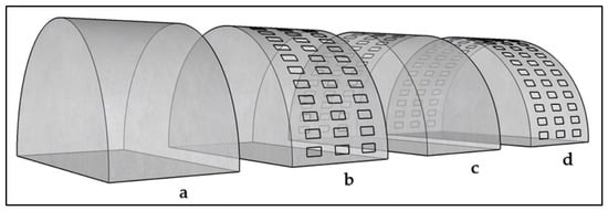
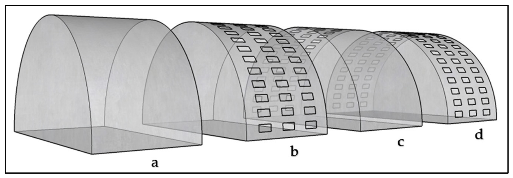
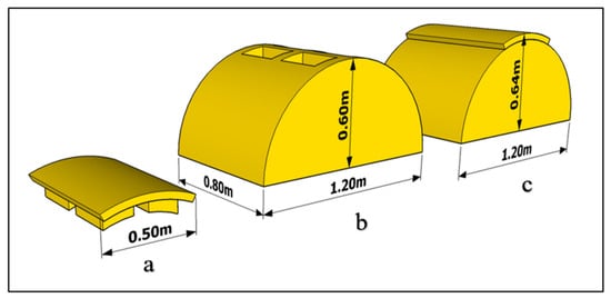
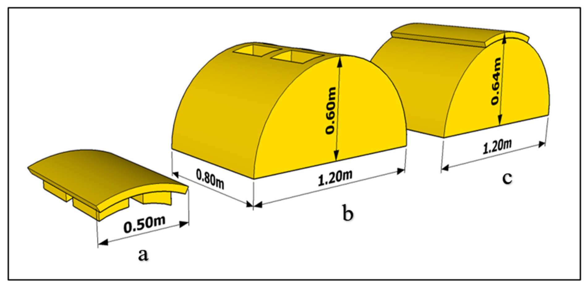
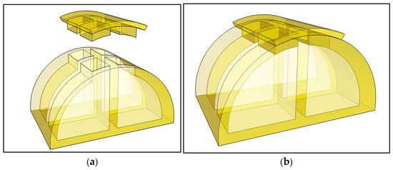
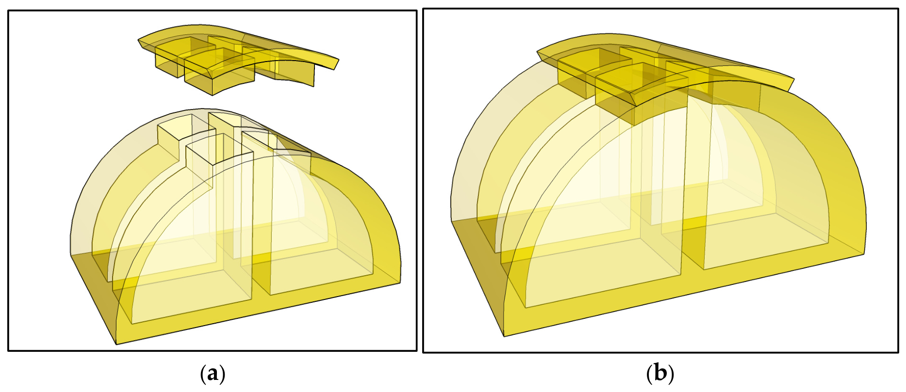
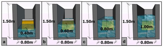
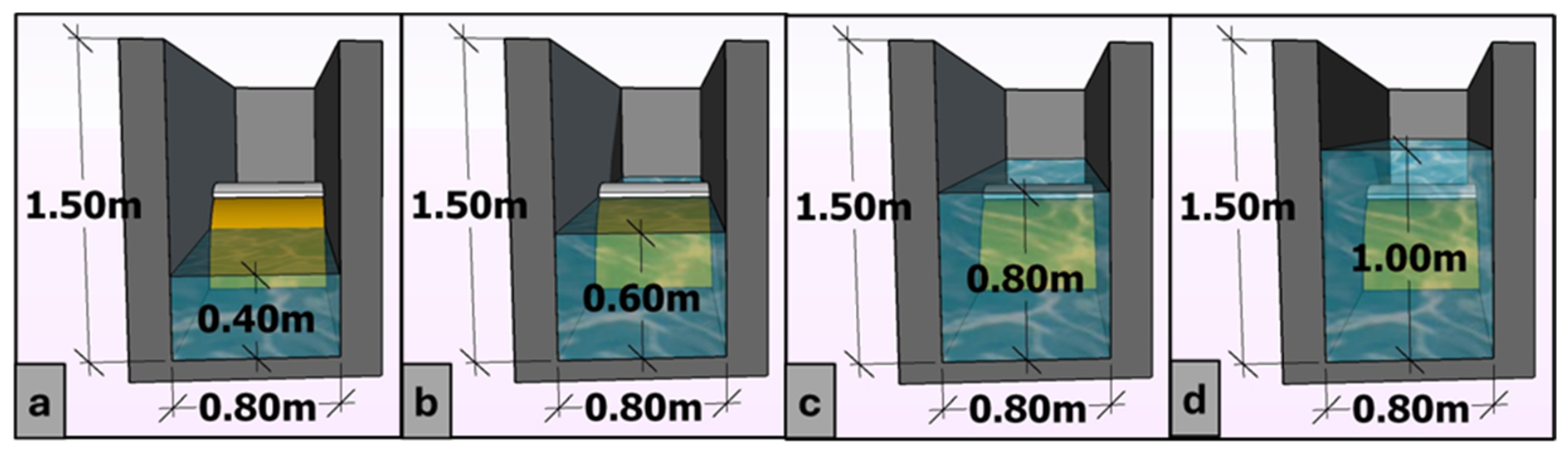
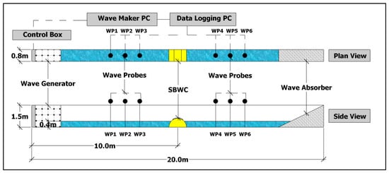
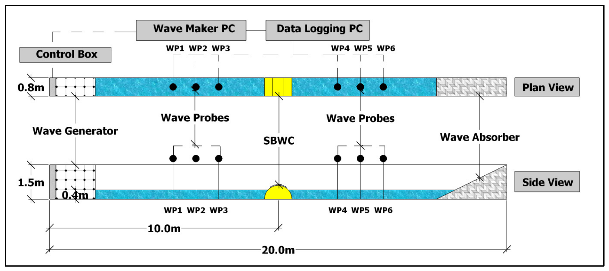
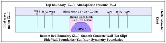
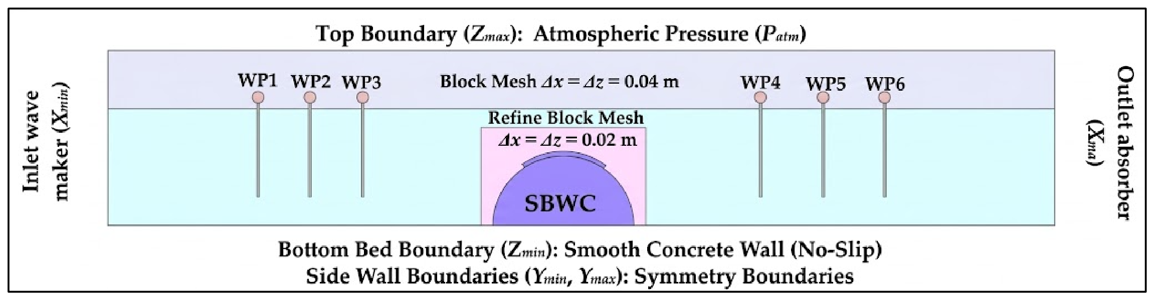
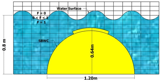
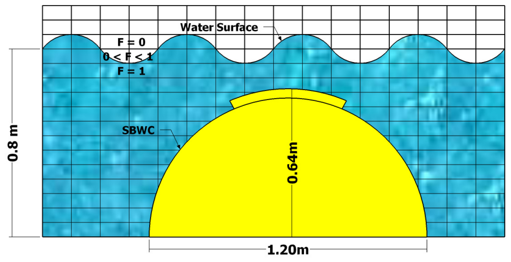
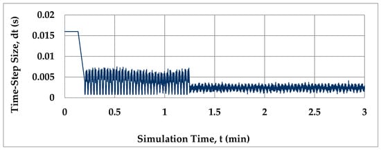
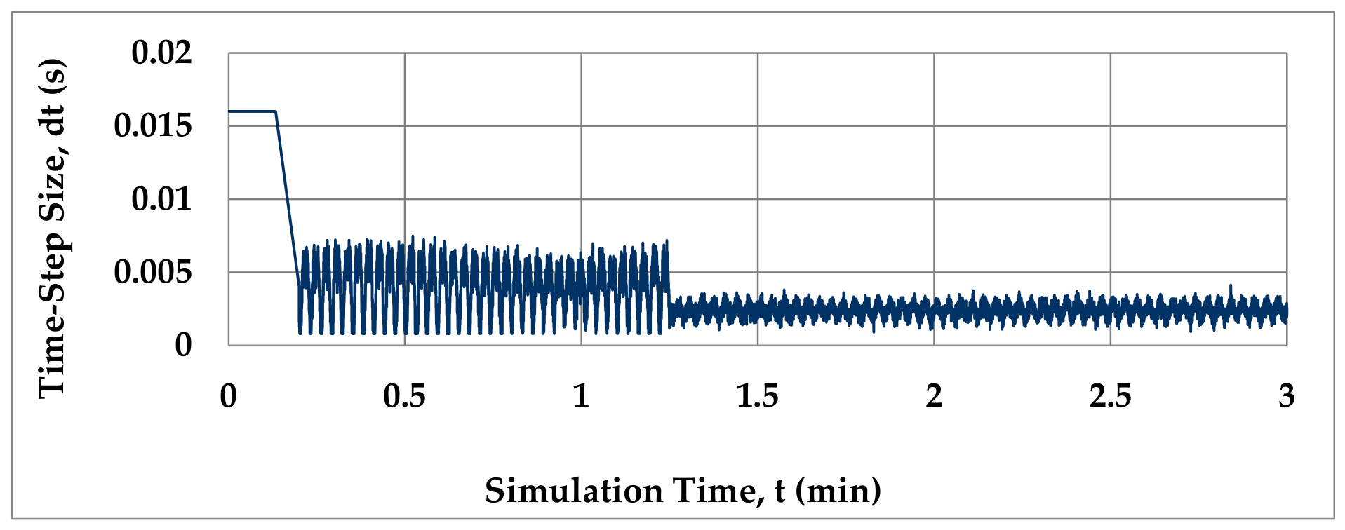
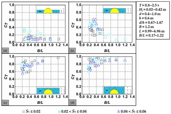
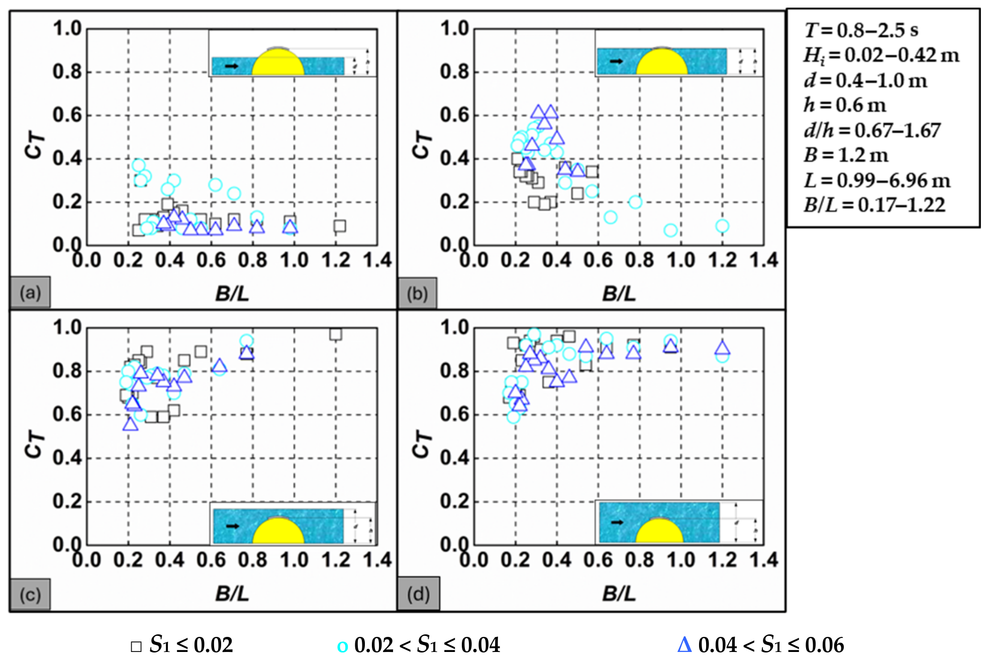
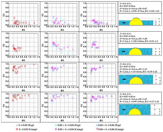
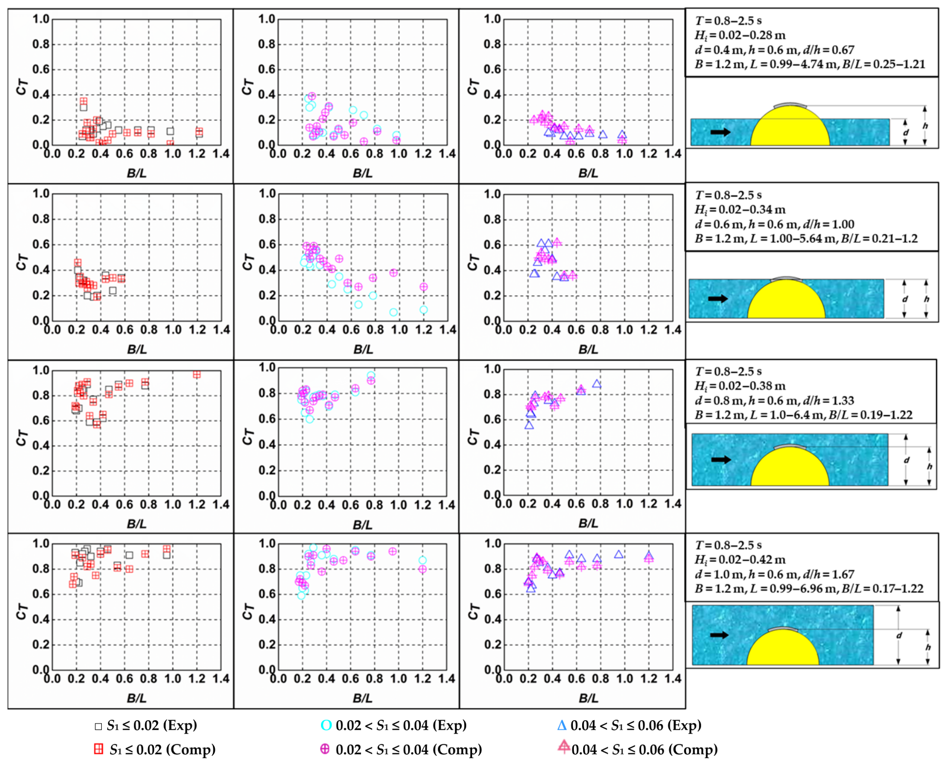
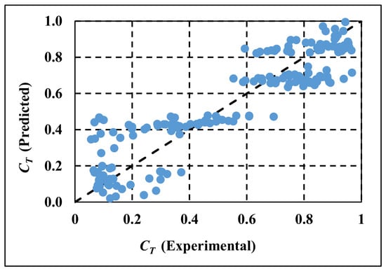
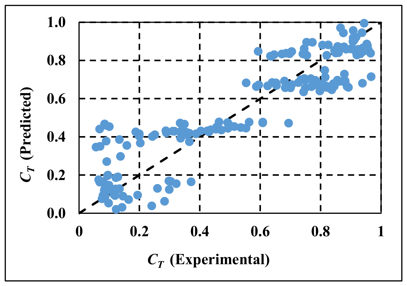
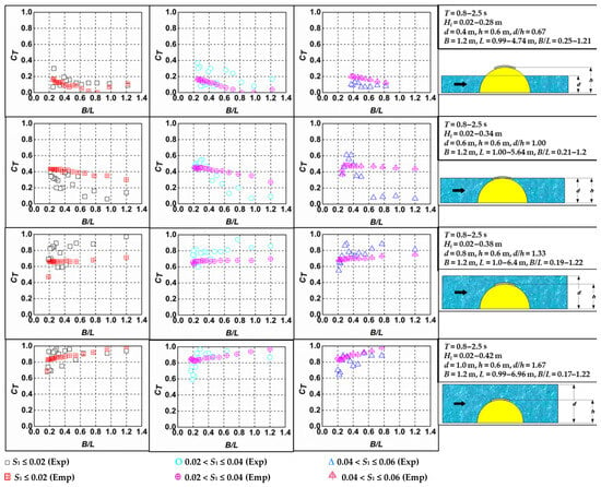
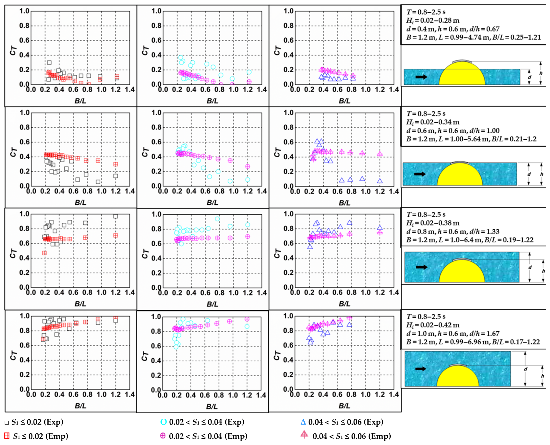
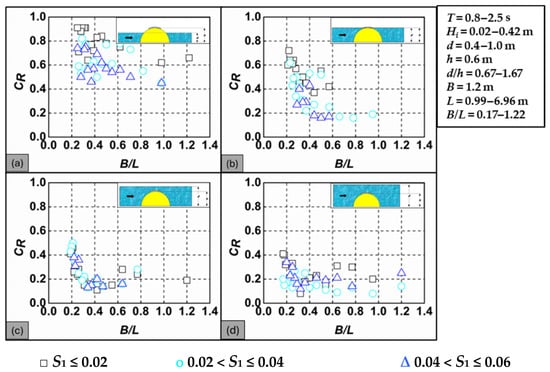
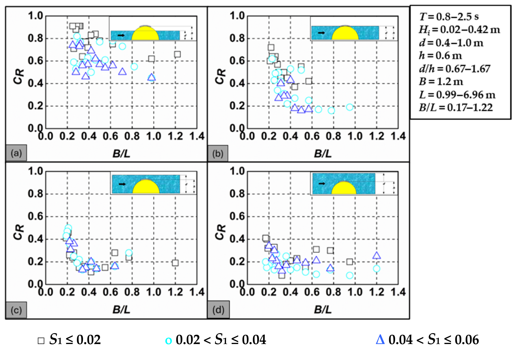
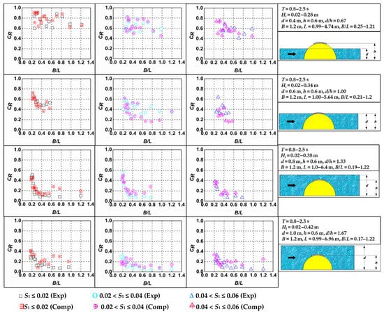
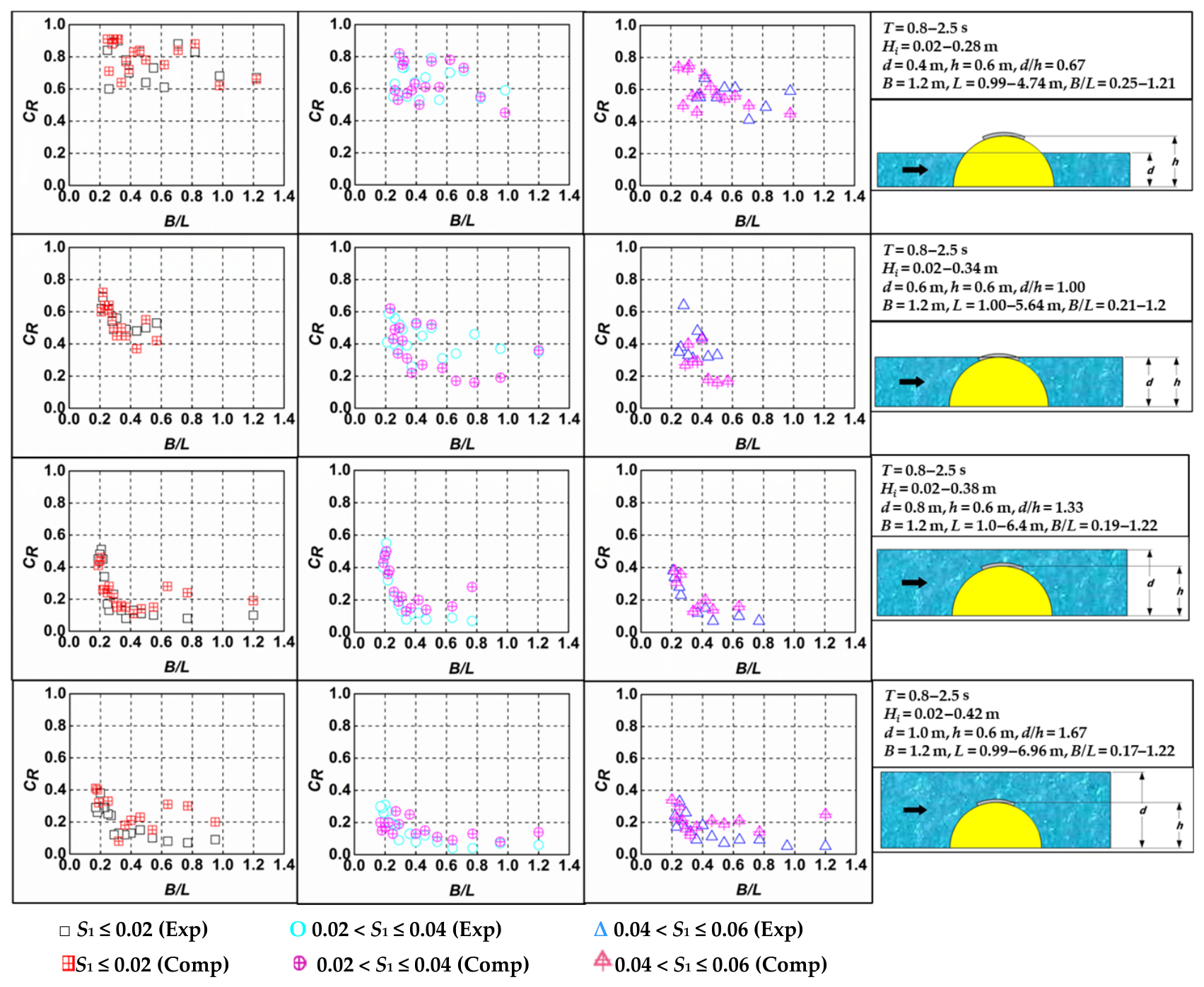
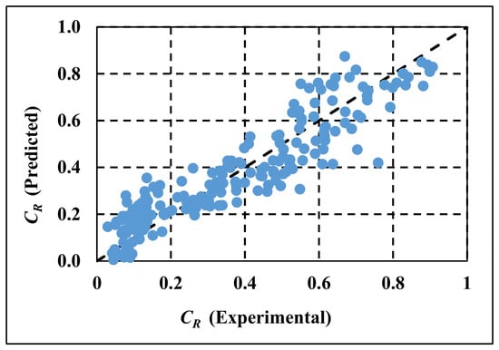
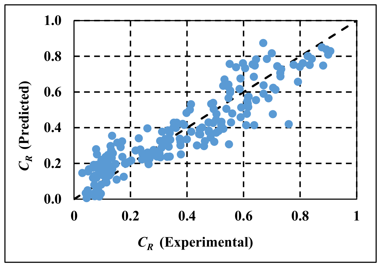
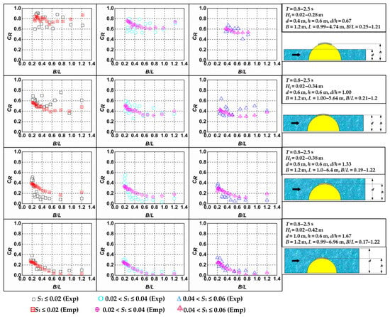
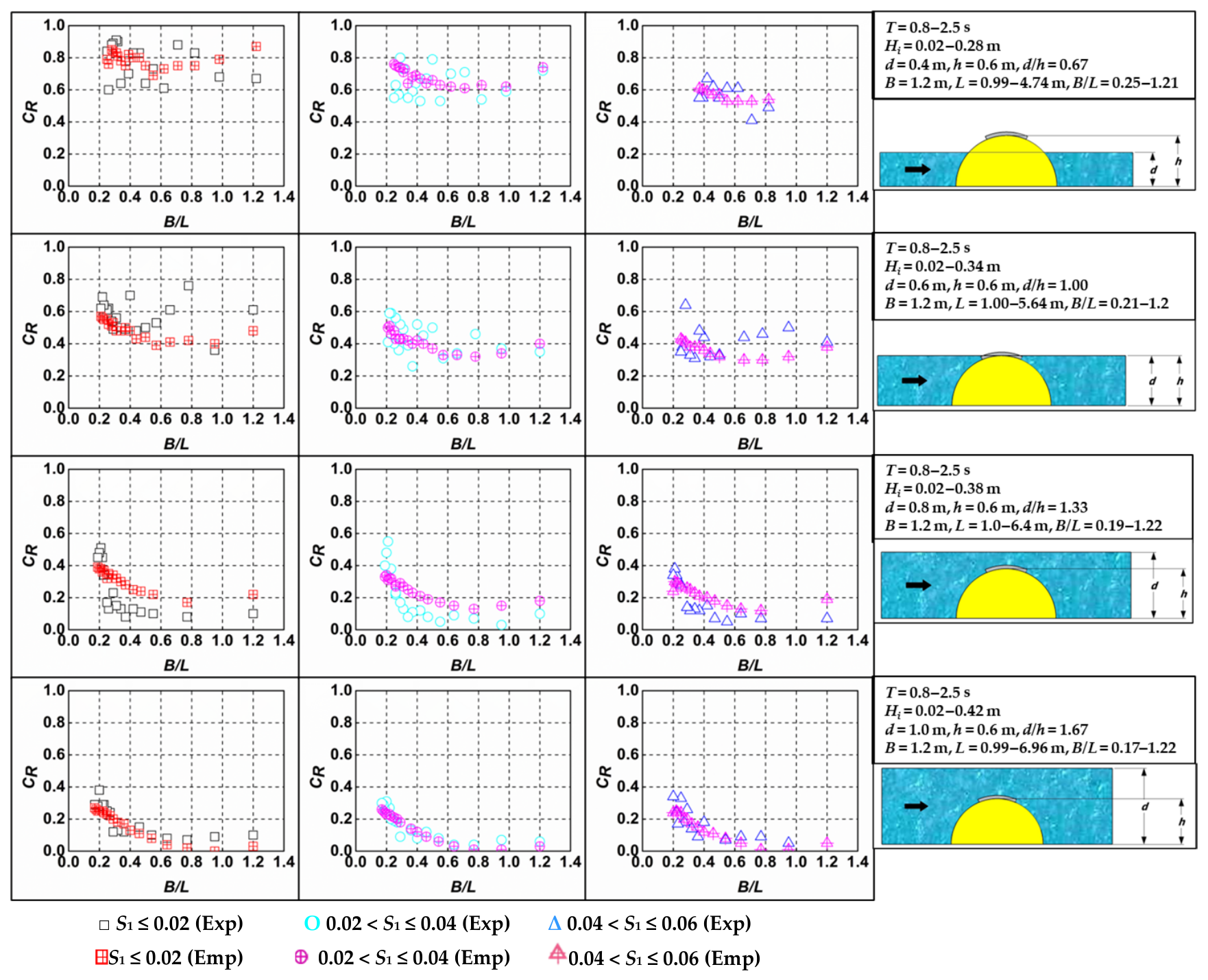
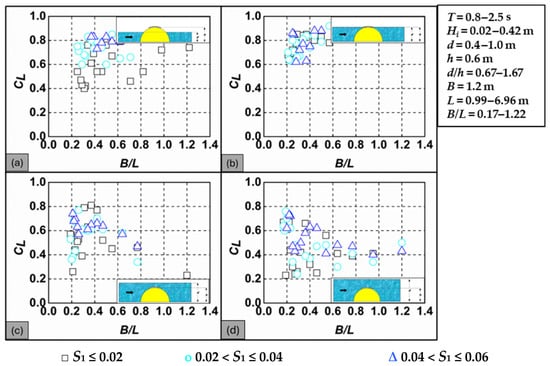
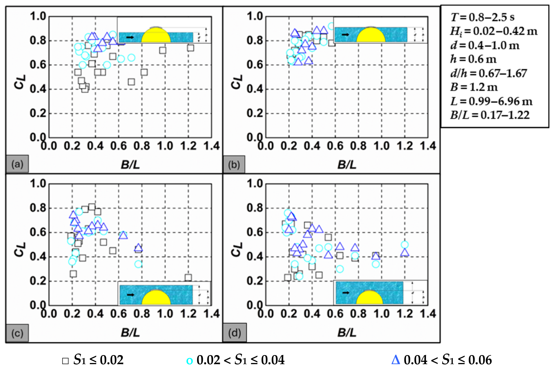
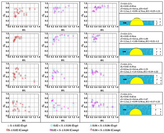
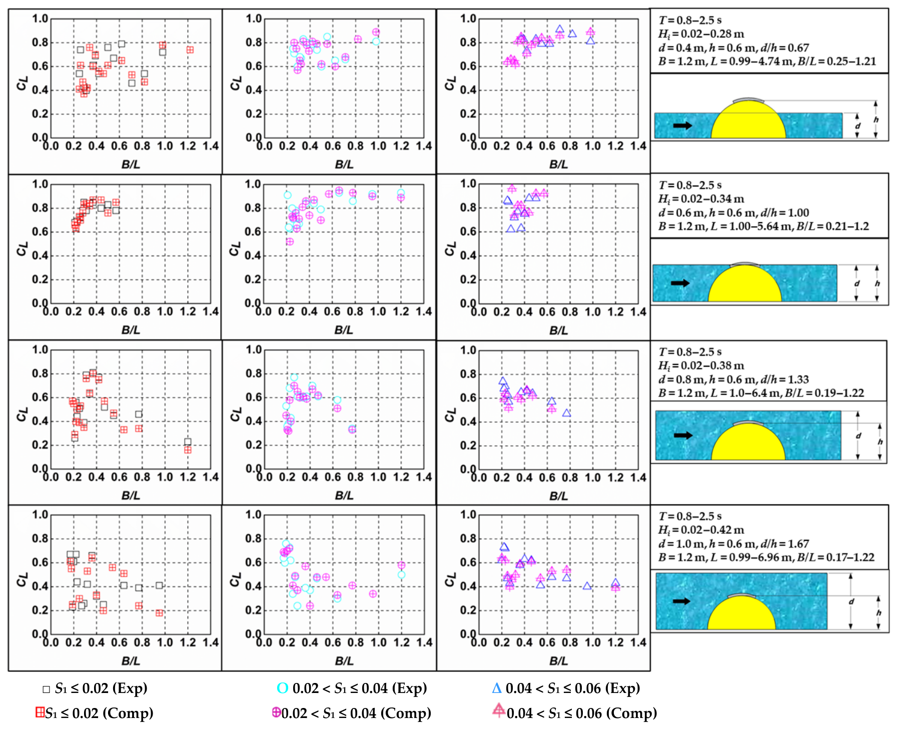
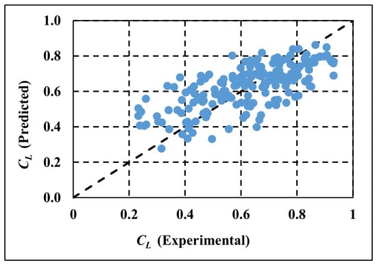
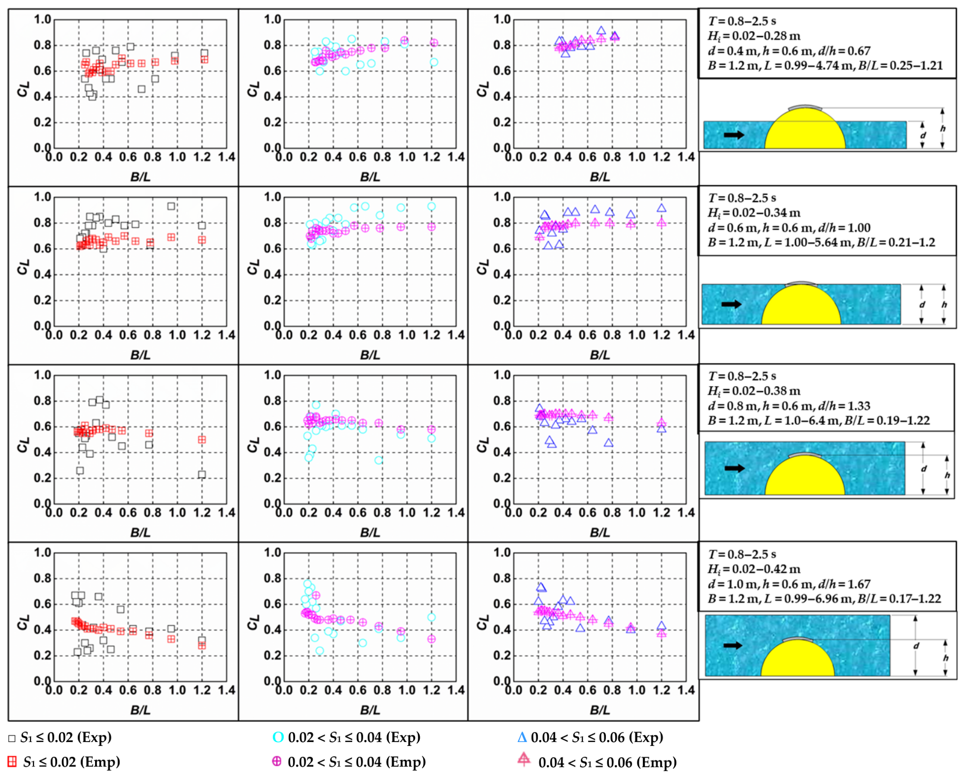
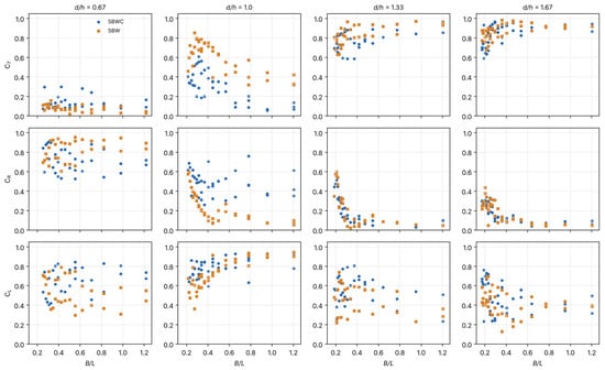
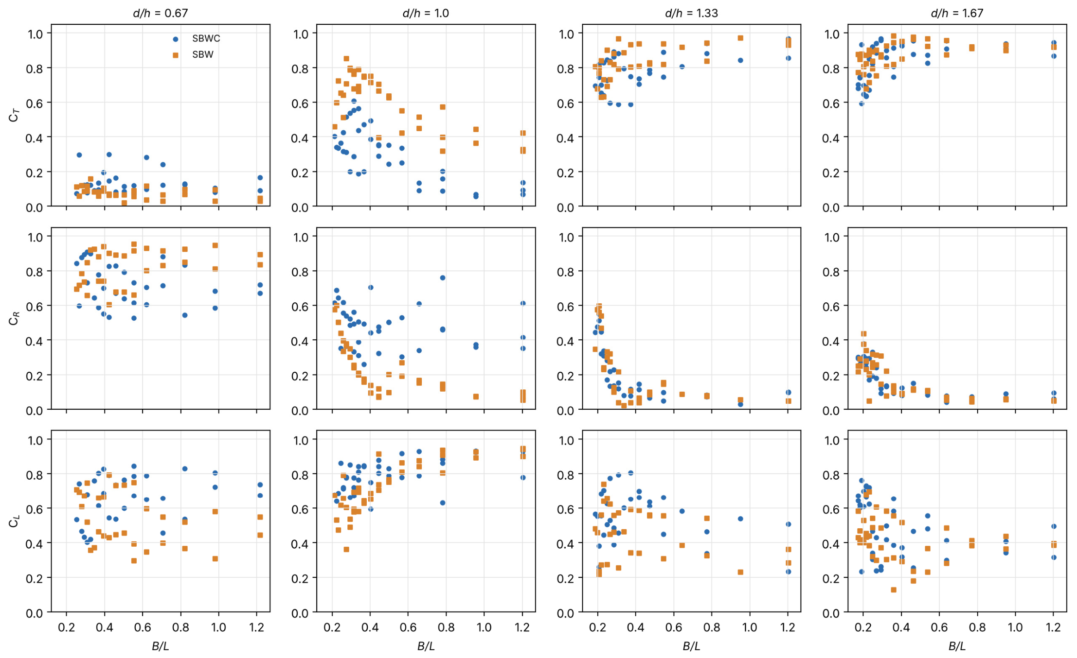
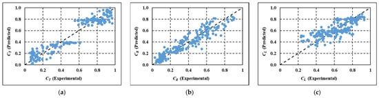
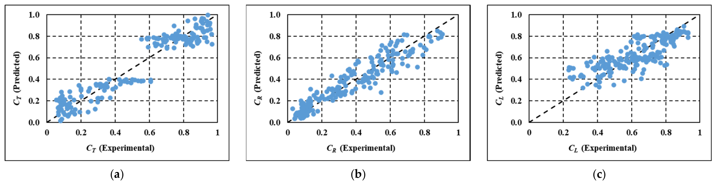

Disclaimer/Publisher’s Note: The statements, opinions and data contained in all publications are solely those of the individual author(s) and contributor(s) and not of MDPI and/or the editor(s). MDPI and/or the editor(s) disclaim responsibility for any injury to people or property resulting from any ideas, methods, instructions or products referred to in the content. |
© 2026 by the authors. Licensee MDPI, Basel, Switzerland. This article is an open access article distributed under the terms and conditions of the Creative Commons Attribution (CC BY) license.