


Abstract
The detection of sea mines in side-scan sonar imagery is hindered by small object size, heavy speckle noise, and severe data scarcity. Existing studies mostly transplant improvements designed for natural images to sonar scenarios, and their effectiveness under small-sample conditions lacks unified verification. This study presents a systematic benchmark of lightweight object detectors on a publicly available side-scan sonar mine-like object dataset, SSS-MLOD. Under a unified protocol, five YOLO variants are compared under from-scratch training and COCO-pretrained transfer learning, and 25 structural, loss-based, and data-side modifications are evaluated. The results show that differences among lightweight baselines are marginal (mAP50 of 0.732 to 0.753), transfer learning on only 243 training images yields the largest single gain (mAP50 from 0.742 to 0.856 for YOLOv13n), and none of the 25 modifications was observed to improve the baseline under from-scratch training on this dataset. Increasing the input resolution improves mAP50:95 by 0.044 to 0.049 for YOLOv5n and YOLOv8n but degrades the performance of YOLOv11n, indicating that the benefit of resolution is architecture-dependent; test-time augmentation with a tuned confidence threshold raises recall by 0.035 under a precision constraint of 0.85. The best configuration, YOLOv13n with transfer learning, achieves an mAP50 of 0.856 and a recall of 0.757. These findings provide an evidence-based reference for detector selection and configuration in resource constrained applications such as autonomous underwater vehicles.
1. Introduction
Sea mines remain a persistent threat to naval operations and maritime traffic, and their rapid and reliable detection is a longstanding requirement for mine countermeasure missions. Deep learning detectors, including YOLO, SSD, and EfficientDet variants, have recently been explored for sea mine detection in sonar imagery [1]. Side-scan sonar (SSS) is one of the most widely used sensors for this task, owing to its high along-track resolution and its ability to survey large areas efficiently [2]. SSS images are formed by recording the backscattered acoustic intensity along the survey track; mine-like objects typically appear as a compact highlight region accompanied by an elongated acoustic shadow cast on the seabed, and this highlight–shadow structure, rather than object texture, constitutes the primary detection cue [3]. The imaging process introduces strong multiplicative speckle noise, which complicates the discrimination between mine-like targets and seabed clutter.
Three characteristics make this task particularly demanding for learning-based detectors. First, training data are scarce: acquiring and annotating SSS imagery requires dedicated survey campaigns, and publicly available mine detection datasets contain only hundreds of images, with annotations requiring domain expertise to distinguish mine-like contacts from natural clutter [4]. Second, targets are extremely small: in the public SSS-MLOD dataset used in this study, 78.1% of the 694 annotated objects have a short side below 32 pixels, with a median size of 24 pixels [4]. Third, mine-like objects possess limited texture and shape diversity; their appearance is essentially a highlight–shadow structure whose contrast varies with acoustic illumination and seabed conditions [3,5,6].
Early SSS target detection relied on template matching and shadow-based reasoning with hand-crafted features, which requires careful tuning under varying seabed conditions [3]. Deep learning methods have since become the dominant approach, as surveyed in [2,3]. Within the YOLO family, Yang et al. [7] proposed SS-YOLO, a lightweight detector combining partial convolution, adaptive scale spatial fusion, and multi-head self-attention for unmanned surface vessel deployment; Cui et al. [8] proposed SOCA-YOLO, which couples image restoration with a small-object convolution module and CBAM attention, and validated generalization on the SSS-MLOD dataset, reporting mAP50 values of 83.7 and 74.3 for SOCA-YOLO and YOLOv9, respectively; Wen et al. [9] combined a diffusion model with an improved YOLOv7 for SSS underwater target detection; and Zou et al. [10] proposed YOLOv11-SDC, which replaces the SPPF module with a sparse feature module and adds dilated reparametrized convolutions. Complementary to these method-oriented studies, a recent evaluation of YOLO variants from v8 to v13 for ocean SSS target detection confirmed large transfer-learning gains across architectures [11].
Transfer learning has proven particularly valuable for this domain. Pretrained networks fine-tuned on limited sonar data can markedly outperform models trained from scratch, as demonstrated for few-sample sonar image classification [12] and in comparative studies of CNN architectures on SSS images [5]. A persistent practical question is how to configure the transfer: freezing the backbone reduces the risk of overfitting but may limit domain adaptation, whereas full fine-tuning adapts all parameters at the cost of a larger optimization space on a small dataset. Self-supervised pretraining on sonar data has also been explored as an alternative to natural-image pretraining [13], motivated by the large domain gap between natural images and sonar imagery.
Methodologically, the small-object nature of mine detection has motivated the transplantation of a rich toolbox from natural-image research, including additional shallow detection heads to raise feature-map resolution, attention mechanisms to reweight salient regions, feature pyramid variants and dynamic upsampling to improve multi-scale fusion, lightweight downsampling operators to reduce information loss, detection-head redesigns, and specialized loss functions that tolerate box-scale sensitivity [8,9,10,11]. On the deployment side, techniques that improve accuracy without retraining have received increasing attention: input-resolution scaling, slicing aided hyper inference and fine-tuning (SAHI) [14], test-time augmentation (TTA), and confidence threshold selection that trades precision against recall at a chosen operating point.
Although the literature is rich, the datasets, training configurations, input resolutions, data splits, and evaluation settings behind published results differ from study to study, which makes cross-study comparison difficult and leaves practitioners without clear guidance on how to combine these design choices on computationally constrained platforms such as autonomous underwater vehicles (AUVs). Motivated by this observation, this study formulates three research questions. RQ1: Under small-sample conditions with a large domain gap, how should transfer learning be configured for SSS mine detection, in particular, is full fine-tuning preferable to frozen-backbone training? RQ2: Without retraining the detector, how much can the inference side—input resolution, TTA, and confidence threshold selection—contribute to detection performance? RQ3: Under a unified protocol, how effective are the structural modifications that are popular in the recent sonar detection literature for this task?
To answer these questions, we present a systematic benchmark of lightweight object detectors on SSS-MLOD, a publicly available dual-class side-scan sonar mine-like object dataset [4]. All experiments follow a fixed training and evaluation protocol with an explicit significance criterion based on the observed run-to-run noise band. Five YOLO variants are compared under from-scratch training and COCO-pretrained transfer learning, and 25 structural, loss-based, and data-side modifications reported in the recent literature are evaluated within the same framework. The results show that inter-generational differences among lightweight baselines are small, whereas transfer learning provides the dominant gain in detection accuracy; the effectiveness of structural modifications is architecture- and domain-dependent, and we identify which modifications provide consistent benefits under controlled conditions; input-resolution scaling benefits older architectures but not newer ones, while jointly tuning TTA and the confidence threshold raises recall by 0.035 under a precision constraint of 0.85. The best configuration, YOLOv13n with transfer learning, achieves an mAP50 of 0.856 and a recall of 0.757, which is the highest value observed under the present protocol and is not directly comparable with the strongest previously published result on this dataset, which was obtained with a different training set and evaluation protocol [8]. These findings directly answer the three research questions and provide an evidence-based reference for detector selection and configuration in resource constrained applications.
The contributions of this study are as follows. First, we establish a unified-protocol benchmark for small-sample SSS mine detection and quantify the inter-generational differences among lightweight detectors, the gain of transfer learning, and the behavior of frozen-backbone training. Second, under controlled conditions, we compare 25 popular structural, loss-based, and data-side modifications on a common baseline, providing reference results for method selection in this domain. Third, we characterize the architecture dependence of input-resolution scaling and derive a low-cost inference-side recipe that combines TTA with confidence threshold selection, yielding a recommended configuration that attains the highest mAP50 observed under the present benchmark protocol.
2. Materials and Methods
2.1. Dataset and Evaluation Protocol
Mine images were sourced from a publicly available dataset comprising 1170 real side-scan sonar images [4]. The data were collected in situ between 2010 and 2021 using a 900–1800 kHz Marine Sonic dual-frequency side-scan sonar (Marine Sonic Technology, Ltd., White Marsh, MD, USA) mounted on a Teledyne Marine Gavia autonomous underwater vehicle. In addition to mine targets, the dataset contains numerous small rocks and complex terrain features. Because most images contain no target instances, only images containing targets were retained, resulting in a final set of 304 samples with 694 annotated objects after removing zero-size annotation errors. The class distribution is 459 MILCO and 235 NOMBO instances. As shown in Table 1, the objects are extremely small: the median short side is 24 pixels, 78.1% of objects have a short side below 32 pixels, and 17.8% below 16 pixels. Images are resized to 640 × 640 for the main experiments, following the standard protocol of the YOLO family. MILCO denotes mine-like contacts, whereas NOMBO denotes non-mine bottom objects. Targets are annotated as bounding boxes, and object short side is defined as the smaller of the annotated box width and height in pixels. Images with zero-size boxes are removed during quality control. Resampling, duplication, or class weighting is not used to alter the natural class distribution. The imbalance between MILCO and NOMBO is instead taken into account by stratified sampling at the splitting stage, so that both classes keep comparable proportions in the training and validation parts. All experiments use the same images, annotation rules, and preprocessing settings. The typical partial dataset samples of the paper used is shown in Figure 1, while the blue square indicates NOMBO, and the red square is MILCO.
Table 1.
Statistics of the SSS-MLOD dataset.
Figure 1.
The typical partial dataset samples of the paper used.
The dataset is divided into 243 training images and 61 validation images (8:2 split). Because the dataset is small and no official test split exists, all reported results are validation-set results. The 8:2 ratio is a pragmatic choice that retains 243 images for training while preserving 61 images for consistent evaluation, rather than a theoretically optimal value. A smaller training share would further reduce the already limited sample and increase sensitivity to individual images. Using one fixed split for all configurations also prevents split variation from being confounded with differences between methods. This allocation follows the general need to balance model fitting and held-out evaluation [15]. Stratified sampling is applied over the annotated instances, which keeps the ratio between MILCO and NOMBO close in the two parts and avoids shortages of either class in the validation part. The validation split is used for early stopping, checkpoint selection, confidence threshold selection, and final reporting, so the reported numbers may be somewhat optimistic and are best interpreted as comparative indicators rather than absolute field performance.
Detection performance is evaluated with precision (P), recall (R), mAP50, and mAP50:95. Following the standard validation protocol of the YOLO family, mAP metrics are computed from the precision–recall curve swept over confidence scores, with 0.001 used as the lower bound of the sweep; the default operating threshold of 0.25 is used only where explicitly stated. The IoU value of 0.7 is used only for non-maximum suppression where NMS is applied. It is distinct from the detection-matching thresholds, with mAP50 calculated at IoU 0.5 and mAP50:95 averaged over IoU thresholds from 0.50 to 0.95 in steps of 0.05. Because all experiments are conducted with a single random seed, we account for training variance explicitly: repeated-run studies on object detectors show that mAP can vary by approximately 0.02 across seeds on small datasets [16]. We therefore treat differences in mAP50 below 0.02 as indistinguishable from run-to-run variance and interpret them as trends rather than meaningful effects.
The public release of SSS-MLOD also contains empty seabed frames without any annotated target. These frames were excluded when the benchmark set was prepared, because they provide no labelled instances for training and no target recall to measure. False alarm behavior on empty seabed is therefore not evaluated in this study, and a dedicated false alarm assessment based on those frames is left as future work. The split is an image-level random split under a single random seed, and adjacent frames from the same survey line may appear in both the training and validation parts. No survey-line or acquisition-time grouping was applied, and the split is therefore not claimed to eliminate spatial or temporal dependence.
To evaluate the detection performance, classical accuracy metrics, such as precision, recall, and mean average precision (mAP), were used to assess the picked results. Referring to the confusion matrix, TP, TN, FP, and FN denote the numbers of true positives, true negatives, false positives, and false negatives, respectively.
Precision is defined as (1):
For class A, precision is defined as the ratio of the number of true positive detections of A to the total number of detections predicted as A.
Recall is defined as the ratio of the number of true positive detections of A to the total number of ground truth objects of A. The calculation of recall is (2):
mAP50 represents the mean of the average precision across all categories calculated at an Intersection over Union (IoU) threshold of 0.5. The calculation formula is shown in Equation (3).
where N represents the total number of categories and APi denotes the average precision of the i-th category. As one of the most commonly used evaluation metrics in the field of object detection, mAP@50 comprehensively considers both precision and recall while measuring localization accuracy with an IoU threshold of 0.5. A higher value indicates superior model performance in the detection task.
mAP50:95 refers to the mean of the average precision values computed for each category at multiple Intersection over Union (IoU) thresholds ranging from 0.5 to 0.95, which are then averaged across all categories. The calculation formula is given in Equation (4).
where M denotes the number of Intersection over Union thresholds (typically 10, ranging from 0.5 to 0.95) and APij refers to the average precision of the i-th category at the j-th threshold. As a more stringent evaluation criterion, the mAP50: 95 metric requires the model to maintain high detection performance across various IoU thresholds. A higher value indicates stronger robustness and accuracy in both target localization and classification tasks.
2.2. Detection Framework
This section describes the methodological object of the benchmark: the single-stage detection framework shared by all baselines, the architectural choices that distinguish the five evaluated generations, and the reference configurations of the neck, head, and loss components. Because every modification evaluated in this study is defined relative to this reference framework, the descriptions below also serve to fix the terminology used throughout the remainder of the paper.
2.2.1. Overall Pipeline
All evaluated detectors follow the single-stage design that has become the standard choice for real-time sonar target detection [17,18]. Each detector consists of three components, namely a backbone that extracts hierarchical feature maps from the input image, a neck that fuses multi-scale features, and a detection head that predicts object classes and bounding boxes at multiple feature-map scales. Given an input image resized to 640 × 640, the backbone produces feature pyramids at strides of 8, 16, and 32, corresponding to the P3, P4, and P5 levels. The neck aggregates information across these levels so that each prediction scale retains both fine spatial detail and high-level semantics, and the head then decodes a class probability and box coordinates for each candidate location. Post-processing removes duplicate predictions through non-maximum suppression, except in YOLOv10n, which replaces this step with a one-to-one assignment branch [19]. Because all five baselines share this general pipeline, the comparison is restricted to single-stage detectors. However, each model retains its reference augmentation pipeline, so the experiments compare complete detector configurations and do not isolate architecture as the sole cause of performance differences.
2.2.2. Backbone Designs
The five baselines represent three generations of backbone design [18,20]. YOLOv5n [17] adopts the CSPDarknet backbone, in which cross-stage partial connections split the feature flow of each stage to reduce computation while preserving gradient diversity. Its basic block is the C3 module, a convolutional bottleneck with a split-and-concatenate branch. YOLOv8n and YOLOv10n share the C2f module, which generalizes the C3 design by connecting all bottleneck outputs in parallel and concatenating them, enriching gradient flow at a comparable cost. YOLOv11n introduces the C3k2 module, which embeds two parallel small-kernel bottlenecks inside the cross-stage framework and simultaneously removes one stage from the backbone, shifting capacity toward the early high-resolution stages that carry the discriminative evidence for small objects [18]. YOLOv13n [11,18] retains the C3k2-based backbone of YOLOv11n with further width adjustments. These design differences matter for the present task because the extremely small target scale, with a median short side of 24 pixels at 640 × 640 input, places the burden of evidence on the early stages of the network.
2.2.3. Neck and Head Designs
The necks of the five baselines build on the feature pyramid structure with a bidirectional path aggregation design [18,19]. A top-down path fuses semantic information into shallow layers, and a bottom-up path propagates localization detail back to deep layers. YOLOv5n and YOLOv8n use an FPN-PAN neck with the CSP bottleneck, YOLOv10n and YOLOv11n adopt lighter necks consistent with their backbone compression, and YOLOv13n follows the same layout as YOLOv11n. All baselines use a decoupled head that separates the classification and regression branches into two parallel convolutional stacks, a design that improves convergence compared with the coupled head of early YOLO versions [19]. YOLOv8n and later variants operate anchor-free, where each grid cell directly regresses distances from the target center to the four box edges, removing anchor hyperparameter tuning that would otherwise be fragile on a dataset of only 243 training images [18]. YOLOv10n additionally adopts a dual assignment scheme with one-to-many labels for training efficiency and one-to-one labels for inference, eliminating non-maximum suppression and its latency [19]. The spatial pyramid pooling module, in its fast variant with successive dilated pools, enlarges the effective receptive field and precedes the neck in all five baselines, and it constitutes the insertion point for several evaluated modifications.
2.2.4. Loss Functions
The baselines share the task-partitioned loss formulation common to recent single-stage detectors [18,19], consisting of a box regression term, an objectness or distribution term, and a classification term. YOLOv5n regresses boxes with the complete intersection-over-union loss and predicts objectness by binary cross-entropy. YOLOv8n and later variants replace the box loss with the distribution focal loss, which models box coordinates as discrete distributions instead of point estimates and has been shown to improve localization of small and ambiguously bounded objects [19]. Classification in all variants is trained with binary cross-entropy. Because the loss design interacts with the specialized loss modifications evaluated later, the baseline losses are kept in their reference configuration throughout this study.
2.3. Transfer Learning
2.3.1. Transfer Learning by Pretraining and Fine-Tuning
Transfer learning reuses knowledge acquired in a source domain to improve learning in a target domain where annotated samples are scarce. In deep learning-based object detection, it is typically realized through a pretraining and fine-tuning paradigm. Although the source domain, represented here by large-scale optical image datasets such as COCO [21], and the target domain, namely SSS imagery, differ in imaging mechanism and data distribution, low-level visual features such as edges, local contrast, and blob-like structures exhibit a degree of universality, so that hierarchical representations learned from abundant source data provide an informative starting point for the target task.
From an optimization perspective, fine-tuning from pretrained weights can be viewed as a search for a solution to the target task in the vicinity of the source-domain optimum [22]. Compared with random initialization, this starting point lies in a more favorable region of the parameter space, which typically accelerates convergence and reduces overfitting on small target datasets [22]. The appropriate depth of adaptation depends on the amount of target data: full fine-tuning exploits all parameters when the target set is moderately sized, whereas freezing shallow backbone layers and updating only the higher-level parameters becomes an option in extremely data-scarce regimes [11,22]. Because a dataset of this size meets the applicable conditions of both regimes, this study evaluates them side by side rather than assuming one to be preferable.
Formally, let the pretrained parameters be θ = (θb, θn, θh), corresponding to the backbone, neck, and head of Section 2.2. Full fine-tuning initializes the network with θ and updates all parameters jointly by minimizing the detection loss of the target task over the whole parameter space. Pretraining contributes an initial point whose early filters encode generic local operators, while every stage remains free to re-adapt to the sonar domain. The effectiveness of this paradigm under limited sonar data has been documented in [5,12], and the multi-variant evaluation in [11] reports it as the dominant accuracy factor across YOLO generations, which motivates its systematic examination in this benchmark.
To separate the effect of pretraining from other factors, the transfer learning experiments use exactly the same training configuration as the from-scratch experiments in all other respects, differing only in the initialization. The comparison between the two paradigms therefore measures the value of the pretrained representation itself rather than of any accompanying change in the optimization procedure.
2.3.2. Frozen-Backbone Fine-Tuning
Frozen-backbone fine-tuning restricts the parameter update to a subset of the network. The parameters of the early backbone stages are fixed at their pretrained values, and the optimization is carried over the remaining parameters only. The underlying assumption is a hierarchy of feature genericity: early stages are believed to encode domain-agnostic local operators, such as edge and contrast detectors, whose re-estimation on a small noisy target set would inject variance without benefit, whereas domain-specific adaptation is delegated to the later stages, the neck, and the head [22]. Frozen-backbone fine-tuning is therefore important as a controlled means of retaining pretrained early features and reducing the number of parameters updated on a small target dataset. It may limit overfitting, but it can also restrict adaptation when the source and target domains differ substantially, so its benefit must be evaluated rather than assumed.
Whether this assumption holds under a large domain gap is an open question. Theoretical and empirical studies show that full fine-tuning distorts pretrained features and can underperform partial adaptation when the distribution shift is large [23], and that fine-tuning only the layers most relevant to the target task, which is closely related to selective freezing, improves adaptation under distribution shifts [24]. These findings suggest that the freezing boundary is a decisive methodological choice rather than a mere implementation detail, and that its optimal position depends on the size of the domain gap, which motivates its controlled examination on sonar imagery.
The freezing sweep examines three freezing depths, namely the first 4, 6, and 10 layers of the backbone. The deepest boundary covers the stem and the first three backbone stages. This depth corresponds to the low-resolution portion of the feature hierarchy, below the level at which the smallest annotated objects (median short side of 24 pixels) are resolved, so the frozen portion is confined to generic preprocessing while every layer that represents object-level evidence remains trainable. The frozen parameters are excluded from gradient updates and weight decay, while the trainable remainder follows the standard optimization procedure. The three depths represent early, intermediate, and nearly complete backbone freezing. Following the Ultralytics layer definitions, freezing 4 layers covers indices 0 to 3 and ends at the downsampling stage for P3, freezing 6 layers covers indices 0 to 5 and ends at the downsampling stage for P4, and freezing 10 layers covers indices 0 to 9 through the P5 backbone stage and SPPF. P3, P4, and P5 correspond to strides 8, 16, and 32, respectively. The neck and head remain trainable in all cases.
2.4. Evaluated Modifications
To answer RQ3, we evaluate 25 modifications drawn from the recent small-object detection literature. All modifications are applied to the YOLOv11n baseline of Section 2.2 and trained from scratch under the protocol of Section 3, except where stated otherwise. This section defines each modification and its methodological motivation; the modifications are presented in six groups, ordered from the data side toward the prediction stage.
2.4.1. Data-Side Methods
The first group modifies the training data rather than the network. Copy–paste augmentation [25] transfers annotated objects into new background regions, increasing the diversity of object–seabed combinations; we evaluate two variants, namely mask-aware pasting that follows the object contour and rectangular pasting that follows the bounding box. Sliced training [14] partitions training images into overlapping tiles, which increases the effective pixel area occupied by each object; because predictions must be reassembled for whole-image evaluation, we assess both in-slice and whole-image validation protocols. The Frangi filter [26] enhances ridge-like structures by analyzing the eigenstructure of the Hessian at multiple scales; applied to SSS imagery, it accentuates the elongated acoustic shadows of mine-like objects [6], and we evaluate two variants, one restricted to target strips and one applied globally.
2.4.2. Backbone Blocks
The second group replaces the C3k2 basic block of the backbone with alternative computational units. The EfficientViM block [27] introduces state-space modeling with a hidden-state mixer that couples spatial scanning with channel mixing; we evaluate two replacement depths, namely all backbone stages and the last two stages. The Monte Carlo attention block [28] generates attention maps by randomly selecting among candidate pooling scales, a stochastic scheme intended to capture scale-variant context for small objects; it is evaluated at the same two depths. The visual state space block [29] applies selective state-space scanning along the spatial dimensions, modeling long-range dependency with complexity linear in the number of positions. The DCNv4 block [30] replaces the dense grid sampling of standard convolution with dynamic sparse sampling whose offsets are predicted from features; we apply it to the last two backbone stages, where receptive-field adaptability is most relevant to shadow localization.
In addition to the four block replacements above, two further backbone configurations are evaluated. C2PSA-Mona replaces the attention operator inside the C2PSA block of YOLOv11n with the Mona attention operator reported in the recent small-object detection literature [31], and it is evaluated both from scratch and from COCO-pretrained weights in order to examine its interaction with transfer learning. The StripShadow block is designed to model the elongated, strip-like acoustic shadows that accompany mine-like objects, and replaces the C3k2 basic block in the backbone.
2.4.3. Neck Structures
The third group modifies the feature-fusion neck. The attentional scale sequence fusion module from ASF-YOLO [32] fuses features across consecutive scales with an attentional sequence rather than plain summation. The lightweight group attention gate (LGAG) [33] replaces direct concatenation in the fusion path with grouped-attention gating, selectively transmitting informative signals with a small parameter overhead. DySample [34] replaces nearest-neighbor upsampling with a content-adaptive operation that learns sampling offsets directly from features, sharpening the reconstruction of small-object detail. The hierarchical semantic fusion pyramid network (HSFPN) [35] screens low-level features with high-level semantics before fusion, suppressing background responses in shallow layers. The bidirectional feature pyramid network (BiFPN) [36] replaces unweighted addition with learnable bidirectional weighted fusion, normalizing feature contributions across resolutions.
2.4.4. Detection Heads
The fourth group modifies the prediction stage. DyHead [37] unifies scale-aware, spatial-aware, and task-aware attention in a single head by applying sequential self-attention over the level, spatial, and channel dimensions. The parallelized patch-aware attention head [38] aggregates contextual features at patch granularity in parallel branches, enlarging the receptive field of the head without deep stacking. We additionally include two structural variants of the reference head that isolate the role of scale coverage: an added P2 detection head that raises the finest prediction stride from 8 to 4, and a head with the coarsest P5 level removed.
2.4.5. Loss Function Improvement
The fifth group replaces the box regression loss of the baseline. AdaFocal [39] adapts the focal weighting to calibration statistics gathered during training, reshaping the loss curvature as the model’s confidence distribution evolves. The scale-based dynamic loss [40] reweights the scale and localization terms of the regression objective according to object size, reducing the sensitivity of small boxes to annotation noise. The normalized Gaussian Wasserstein distance loss (NWD) [41] models each box as a two-dimensional Gaussian distribution and measures the distance between boxes in Wasserstein space, which prevents large boxes from dominating the regression gradient on the small-object regime.
2.4.6. Convolutional Operators
The sixth group replaces the downsampling and basic convolution operators of the backbone. HPDown [42] performs downsampling through a hybrid of max and average pooling applied to channel-halved branches, preserving small-object detail while reducing computation. The multi-feature aggregation operator (MFA) [43] aggregates multi-frequency responses of the input feature map, enriching texture representation with a single convolutional group. SPDConv [44] replaces strided convolution and pooling with a space-to-depth transformation followed by non-strided convolution, retaining all spatial information through the downsampling step.
2.5. Input Resolution and Deployment Settings
2.5.1. Input Resolution Scaling
The input resolution determines the pixel extent of the smallest detectable object. At the reference resolution of 640 × 640, the P3 prediction level, with a stride of 8 pixels, represents the median object (short side of 24 pixels) by only three positions per axis, and objects below 16 pixels occupy less than one stride; the fine detail that distinguishes a target highlight from speckle is therefore largely committed to the earliest downsampling steps. Increasing the resolution to 1280 × 1280 doubles the linear extent of every object, so the median target spans six positions at P3 and the smallest annotated objects become resolvable at the standard detection scales. All four evaluated architectures are retrained at 1280 × 1280 under an otherwise identical configuration, so that the effect of resolution is measured independently of the training protocol.
2.5.2. Test-Time Augmentation
Test-time augmentation improves robustness without retraining by aggregating predictions over multiple transformed views of the same image. In this study, TTA is implemented as a horizontal flip of the input image; the resulting predictions are transformed back to the original coordinates and merged with the direct predictions. A detection is retained if it is confirmed by the weighted non-maximum suppression across both views, with the confidence scores averaged; this ensembling suppresses view-specific false alarms while reinforcing detections that are stable under mirroring. Mirroring is chosen because the acoustic shadow of a mine-like object is directional, and a horizontally mirrored view presents the classifier with the shadow geometry of targets surveyed from the opposite side.
2.5.3. Confidence Working-Point Selection
The confidence threshold converts the continuous output of the detector into a binary decision, and its value defines an operating point that trades precision against recall. Because mine countermeasure screening is asymmetric—a missed target carries a substantially higher operational cost than a false alarm that is later cleared by a second pass—we select the operating point by constrained optimization rather than by the detector default. Concretely, the confidence threshold is swept across a dense grid on the validation set, the precision and recall of each candidate threshold are recorded, and the operating point is chosen as the threshold that maximizes recall subject to a precision constraint of P ≥ 0.85. The same procedure is applied with and without TTA, which yields two operating points; the final deployment configuration is the pair (TTA setting, confidence threshold) with the highest constrained recall. All thresholds reported in Section 3 refer to this validation-based selection, and the selected values are candidates for confirmation on additional data before field deployment.
3. Experiments and Results
3.1. Experimental Setup
All experiments are conducted with the YOLO framework (Ultralytics) under a single unified configuration, summarized in Table 2. The input resolution is 640 × 640 for the main experiments, with a separate 1280 × 1280 group reported in Section 3.4. Optimization uses stochastic gradient descent with an initial learning rate of 0.01, momentum of 0.937, and a batch size of 16; the learning rate follows a linear decay schedule after a warm-up phase, and cosine annealing is disabled so that every model experiences the same effective learning-rate trajectory. Training runs for at most 2000 epochs with early stopping triggered by the patience of the validation mAP50, a budget that is generous relative to the dataset size and ensures convergence of all baselines. The random seed is fixed to 0 for all experiments. Seed 0 was selected arbitrarily for reproducibility and not by comparing performance across seeds. It controls random initialization, data shuffling, and stochastic augmentation. Using the same seed for all configurations provides a consistent comparison but does not estimate run-to-run variability. Training is performed on a single NVIDIA GeForce RTX 4060 Laptop GPU with PyTorch 2.1.1, CUDA 11.8 and Ultralytics 8.3.13.
Table 2.
Unified training and evaluation configuration.
Each model’s default data augmentation pipeline is retained unchanged, because the augmentation policy is part of the reference configuration of the detector; no additional augmentation is introduced at the baseline stage, and data-side modifications are evaluated separately in Section 3.5. From-scratch models are initialized with random weights, and transfer-learning models are initialized with COCO-pretrained weights and fully fine-tuned, as defined in Section 2.3.1; the frozen-backbone configurations follow Section 2.3.2. All modifications of Section 2.4 are applied to the YOLOv11n baseline and trained from scratch unless stated otherwise. This controlled choice isolates the net effect of each modification from the shared pretraining gain quantified in Section 3.2, and the corresponding conclusions are restricted to the from-scratch condition. Retaining the default augmentation pipelines preserves the reference implementation of each detector, but augmentation remains a possible contributor to performance differences. The baseline comparison therefore concerns complete detector configurations rather than architecture alone. Evaluation follows the protocol of Section 2.1, and all results are validation-set results obtained with the mAP sweep lower bound of 0.001 and an NMS IoU threshold of 0.7, except for the deployment working points of Section 3.6, which use the thresholds selected by the procedure of Section 2.5.3.
The experiments are organized around the three research questions. Section 3.2 compares the five baseline detectors under from-scratch training and transfer learning and examines the frozen-backbone configurations (RQ1). Section 3.3 reports the 25 structural, loss-based, and data-side modifications on the common baseline (RQ3). Section 3.4 analyzes the effect of input resolution. Section 3.5 reports the data-side methods, and Section 3.6 evaluates the inference-side deployment settings, namely TTA and confidence threshold selection (RQ2).
3.2. Baseline Comparison and Transfer Learning (RQ1)
This section compares five lightweight baseline detectors under from-scratch training and transfer learning, and examines the effect of frozen-backbone training on transfer learning. Differences are interpreted against the 0.02 reference band defined in Section 2.1, with in-band values treated as trends.
3.2.1. Baseline and Transfer Configurations
This section establishes the reference points for all subsequent experiments. Table 3 reports the from-scratch baselines of the five detectors, and Table 4 reports the corresponding transfer-learning configurations in which each model is fine-tuned from COCO-pretrained weights. Figure 2 visualizes the two tables, showing that the transfer-learning advantage holds for both detection accuracy and localization quality across all five architectures.
Table 3.
Baseline detectors under from-scratch training (640 × 640 input).
Table 4.
Baseline detectors under transfer learning with full fine-tuning (640 × 640 input).
Figure 2.
From-scratch versus transfer-learning performance of the five baseline detectors on the SSS-MLOD dataset. (a) mAP50; (b) mAP50:95.
On this dataset, the from-scratch baselines of the five detectors cluster within a narrow range of mAP50. YOLOv11n achieves the highest value at 0.753, followed by YOLOv13n at 0.742, YOLOv5n at 0.738, YOLOv10n at 0.733, and YOLOv8n at 0.732. Given the ±0.02 noise band associated with single-seed training, these differences are treated as trends rather than significant effects, and the five from-scratch baselines are regarded as roughly comparable in detection accuracy. The spread is wider for mAP50:95, where YOLOv11n leads at 0.610 and YOLOv13n trails at 0.542, indicating that, on this dataset, the models differ more in localization quality across IoU thresholds than in coarse detection accuracy.
Transfer learning improves every detector by a margin that exceeds the noise band, as shown in Table 4. Under the small-sample condition of this dataset, the gains in mAP50 range from +0.041 for YOLOv11n (0.794) to +0.114 for YOLOv13n (0.856), with YOLOv8n gaining +0.064 (0.796), YOLOv5n +0.052 (0.790), and YOLOv10n +0.045 (0.778). The recall response to transfer learning is more heterogeneous across architectures. On this dataset, YOLOv13n reaches a recall of 0.757 under the official validation protocol, the highest among all configurations in this study and +0.099 above its from-scratch value; YOLOv5n and YOLOv10n also gain recall beyond the noise band (+0.068 to 0.727 and +0.043 to 0.704, respectively), whereas YOLOv8n changes by +0.035 (0.701 versus 0.666) and YOLOv11n slightly decreases (−0.025, 0.671 versus 0.696). These results support two conclusions on this dataset, with the same single-seed caveat as above.
First, transfer learning is clearly beneficial under the small-sample condition of this dataset for all five architectures, and the size of the benefit is architecture-dependent, varying from +0.041 to +0.114 in mAP50 and from −0.025 to +0.099 in recall. The largest beneficiary, YOLOv13n, also showed the lowest from-scratch mAP50:95, suggesting that on this dataset the detectors that struggle most when trained from scratch gain the most from pretrained weights; this pattern is reported as a trend rather than a validated causal claim. Because missed detections are more costly than false alarms in mine detection, we additionally note that YOLOv13n combines the highest mAP50 with the highest recall under transfer, which makes it the most suitable reference architecture for the miss-sensitive requirement on this dataset. The per-class rows in Table 3 and Table 4 show that MILCO attains higher recall than NOMBO under both training conditions for four of the five architectures, and the two classes are nearly tied for YOLOv13n under transfer learning. Representative qualitative detection examples on the validation set are shown in Figure 3.
Figure 3.
Qualitative detection examples on the SSS-MLOD validation set. Green boxes denote NOMBO and blue boxes denote MILCO.
The importance of YOLOv13n with transfer learning is that it demonstrates how initialization can change architecture rankings: its from-scratch localization result was relatively weak, whereas full fine-tuning produced the highest transfer-learning mAP50 and recall. This finding shows the practical value of evaluating lightweight detectors under both initialization conditions. It identifies YOLOv13n as the best reference configuration under the present dataset and protocol, not as a universally superior architecture. More generally, pretraining reduces the need to learn all visual features from only 243 sonar images, although its effect is not uniform across architectures and metrics.
3.2.2. Frozen-Backbone Configurations
To quantify the cost of freezing under the small-sample condition of the present dataset, we trained YOLOv11n and YOLOv8n with the first backbone layers frozen, following the configuration in Section 2.3.2. Table 5 and Table 6 report the results, and Figure 4 visualizes them with the from-scratch baseline of each model as a reference, with each frozen configuration placed between the from-scratch and fully fine-tuned baselines of the corresponding model for direct comparison.
Table 5.
Frozen-backbone configurations on YOLOv11n.
Table 6.
Frozen-backbone configurations on YOLOv8n.
Figure 4.
Effect of freezing depth on transfer-learning performance. (a) YOLOv11n, mAP50; (b) YOLOv11n, mAP50:95; (c) YOLOv8n, mAP50; (d) YOLOv8n, mAP50:95. Dashed lines mark the from-scratch baseline of each model. On this dataset, both metrics degrade monotonically with freezing depth, and the degradation is substantially larger for mAP50:95 than for mAP50.
For YOLOv11n, freezing the first 4 layers cost 0.024 mAP50 relative to full fine-tuning, and freezing the first 6 layers cost 0.045; freezing the first 10 layers reduced mAP50 to 0.622, below its from-scratch baseline (0.753), indicating that under the small-sample condition of this dataset, transfer learning with deep freezing becomes counterproductive. For YOLOv8n, the degradation was steeper: freezing the first 4 layers already cost 0.053 mAP50, and freezing the first 10 layers (0.555) fell well below its from-scratch baseline (0.732). The recall follows a similar but sharper pattern. For YOLOv11n, the recall stayed close to the from-scratch level of 0.696 under shallow freezing (0.664 at 4 layers, 0.662 at 6 layers) and fell to 0.598 only at 10 layers. For YOLOv8n, by contrast, the recall dropped below the noise band already at 6 frozen layers (0.600) and reached 0.468 at 10 layers, a loss of 0.233 relative to full fine-tuning and the largest recall decline observed in this study. Two observations follow from these results, with the caveat that all runs used a single seed and differences within ±0.02 should be read as trends rather than significant effects.
First, the cost of freezing is graded with depth rather than binary. Shallow freezing (the first 4 layers) retains most of the transfer benefit for YOLOv11n (0.770 versus 0.794 for full fine-tuning), whereas the same configuration removes nearly all of it for YOLOv8n (0.743 versus 0.796). The tolerance to freezing is therefore architecture-dependent, a trend consistent with the different backbone designs of the two models described in Section 2.2.2.
Second, the two metrics degrade at markedly different rates as the freezing depth increases, as shown in Figure 4. For mAP50, shallow freezing keeps both models above their from-scratch baselines (0.770 versus 0.753 for YOLOv11n, and 0.743 versus 0.732 for YOLOv8n), and a clear drop appears only under deep freezing, to 0.622 and 0.555, respectively. For mAP50:95, the decline starts earlier and is far steeper: on this dataset it falls below the from-scratch baseline at a shallower freezing depth than mAP50 does, being already 0.038 below the baseline for YOLOv8n at 4 frozen layers, while YOLOv11n remains approximately at the baseline (0.605 versus 0.610, a difference within the noise band); freezing the first 10 layers reduces mAP50:95 by 0.251 for YOLOv11n and 0.266 for YOLOv8n. These patterns suggest that, on this dataset, freezing primarily harms localization quality across IoU thresholds rather than coarse detection accuracy, and that YOLOv8n is consistently less tolerant to freezing than YOLOv11n on both metrics. In addition, the recall results in this section indicate that, on this dataset, the cost of deep freezing falls primarily on the recall, and that frozen configurations should be screened by recall rather than by mAP50 alone when the deployment is miss-sensitive. The divergence between the two models suggests that the depth at which freezing stops helping is a per-architecture property rather than a universal constant, and the two freezing tables in this section provide reference points for practitioners choosing between frozen and fully fine-tuned transfer on small sonar datasets. Because the freezing sweep was conducted only for two architectures, we refrain from generalizing these depth thresholds to other detectors. The deterioration with deeper freezing suggests that early optical features are not fully sufficient for the sonar domain and that excessive freezing restricts adaptation to speckle, shadow structure, and small-target localization. The stronger declines in mAP50:95 and recall are consistent with degraded localization and increased missed detections, although this mechanism remains an interpretation of the observed results rather than a proven causal effect.
3.3. Structural, Loss, and Convolution Modifications
This section addresses the structural part of RQ3 by evaluating the modifications described in Section 2.4.2, Section 2.4.3, Section 2.4.4, Section 2.4.5 and Section 2.4.6, covering the backbone, neck, detection head, loss functions, and convolution operations. To isolate the effect of each modification from pretrained weights, all modified architectures in this sweep were trained from scratch under the same protocol as the baseline, and the reference for comparison is the from-scratch YOLOv11n baseline (0.753 mAP50, 0.610 mAP50:95). One additional architecture, C2PSA-Mona, was also trained from COCO-pretrained weights to examine its interaction with transfer learning. Table 7 reports the results, with modifications grouped by position and ΔmAP50 computed against the baseline. Unless stated otherwise, the single-seed caveat of Section 3.2 applies, and differences within ±0.02 are read as trends.
Table 7.
From-scratch evaluation of structural, loss, and convolution modifications on YOLOv11n. Values in parentheses are deviations from the from-scratch baseline (P 0.886, R 0.696, mAP50 0.753, mAP50:95 0.610). GFLOPs are measured at 640 × 640 input. Deviations above +0.02 are highlighted in red.
In the backbone group, five of the eleven configurations stayed within the noise band of the baseline on mAP50: C3k2-EfficientViM replacing all blocks (+0.002) or the last two blocks (−0.004), C3k2-MCAttn replacing all blocks (−0.005), CBAM inserted before SPPF (+0.003), and C2PSA-Mona (−0.016). Two placement effects deserve attention. First, MCAttn exhibits a pronounced placement gradient: replacing all C3k2 blocks stayed in the band, whereas replacing only the first two blocks reduced mAP50 by 0.055 and replacing only the last two by 0.070; under the single-seed protocol we report this ordering as a trend rather than a confirmed effect. Second, with the insertion position held fixed at the layer preceding SPPF, the two attention modules produced markedly different outcomes: standalone MCAttn reduced mAP50 by 0.056, whereas CBAM exceeded the baseline by 0.003. The effect of attention insertion at this position is therefore module-specific rather than position-specific. The remaining backbone substitutions fell outside the band on the negative side: C3k2-StripShadow by −0.033, VSSBlock by −0.026, and DCNv4 by −0.031.
Two configurations exceeded the baseline precision by more than the noise band, namely C3k2-EfficientViM replacing the last two blocks (+0.025) and C3k2-MCAttn replacing all blocks (+0.059); in both cases, however, the recall dropped by a comparable margin (−0.031 and −0.061), and the mAP50 remained within the band of the baseline. On this dataset, these precision gains therefore reflect a precision-recall trade-off under the default confidence working point rather than an overall improvement in detection accuracy, and the two configurations are retained in the within-band set in the summary below.
In the neck group, all eight configurations remained below the baseline, with ΔmAP50 ranging from −0.012 (LGAG over three scales) to −0.027 (HSFPN and CSPStage). Two cost observations are worth noting. First, the largest configuration in the sweep, LGAG over three scales, more than doubles the computational cost (16.6 GFLOPs versus 6.3 for the baseline) without a measurable accuracy gain, and restricting LGAG to the small-object scale, which still costs 13.8 GFLOPs, degraded mAP50 by 0.055. Second, DySample and SDFM achieved the highest mAP50:95 values in the neck group (0.584 and 0.581) while remaining below the baseline on both metrics.
In the head group, DyHead stayed within the band of the baseline (−0.004), while Detect-PPA dropped by 0.025. The two head surgeries showed the largest declines in the entire sweep: removing the P5 head reduced mAP50 by 0.084 while lowering the computational cost to 4.5 GFLOPs, and adding a P2 head reduced mAP50 by 0.056 while raising it to 10.2 GFLOPs. On this dataset, altering the number of detection scales therefore degraded accuracy in both directions and was never cost-effective, which is consistent with the small absolute size of the targets, since the P5 head carries few responsible targets and the additional P2 head introduces a lightly supervised branch.
In the loss group, NWD stayed closest to the baseline (−0.015), whereas AdaFocal and SD Loss reduced mAP50 by 0.056 and 0.041, respectively, accompanied by recall drops of 0.082 and 0.083 relative to the baseline recall of 0.696. On this dataset, replacing the default box-regression and classification objectives therefore carries a measurable risk under the from-scratch protocol. In the convolution group, HPDown was closest to the baseline (−0.014) and additionally reduced the computational cost to 5.6 GFLOPs, while MFA and SPD-Conv fell outside the band (−0.043 and −0.026).
Because a missed mine-like target is typically more costly than a false alarm in mine detection, we additionally examine the recall deviations reported in Table 7. On this dataset, no configuration exceeded the baseline recall of 0.696 by more than the noise band. The highest recall among all configurations was achieved by CBAM inserted before SPPF (0.711, +0.015); because this configuration also stays within the mAP50 band, it is the only one that preserves detection accuracy while marginally increasing recall, and it is therefore the most compatible with the miss-sensitive requirement among the configurations evaluated here. A small group of configurations preserved recall within the band, including C3k2-EfficientViM replacing all blocks (−0.007) and ASF (−0.015). The remaining configurations lost recall beyond the band, several by more than 0.05: removal of the P5 head (−0.108), C3k2-MCAttn replacing the first two blocks (−0.101), C3k2-StripShadow (−0.090), LGAG restricted to the small-object scale (−0.087), AdaFocal (−0.082), and SD Loss (−0.083); the two configurations with the largest precision gains also fall in this group (−0.031 and −0.061). For miss-sensitive deployment on this dataset, the configurations in the first two groups are preferable, and the magnitude of the recall deviation should be weighed alongside mAP50 when selecting a modification.
Three observations summarize this sweep on the present dataset. First, none of the 29 configurations exceeded the from-scratch baseline by more than the noise band; the best results, CBAM inserted before SPPF (+0.003) and EfficientViM replacing all C3k2 blocks (+0.002), were statistically indistinguishable from the baseline under the single-seed protocol, and the same held for C2PSA-Mona under transfer learning. Second, the declines were concentrated in three patterns: replacement of the loss objectives, addition or removal of detection scales, and partial substitution of C3k2 blocks in the backbone, whereas several attention modules in band-preserving placements performed on par with the baseline. Third, mAP50:95 was below the baseline for all 29 configurations, the best being DySample at 0.584 versus 0.610, indicating that on this dataset the modifications did not improve, and in most cases reduced, localization quality across IoU thresholds. Relatedly, most configurations that preserved mAP50 did not preserve recall to the same extent on this dataset, and only CBAM inserted before SPPF kept both metrics within the band while marginally increasing recall. These modifications were proposed and validated on datasets considerably larger than the present one, and the results above indicate that their benefits are dataset-conditional rather than universal; we therefore report them as reference points for the small-sample regime rather than as assessments of the original methods.
3.4. Input Resolution
This section addresses RQ2 by evaluating the effect of doubling the input resolution from 640 × 640 to 1280 × 1280 under the from-scratch protocol. Higher resolution preserves more detail of the small targets in this dataset, at a substantially increased computational and memory cost, so it is not obvious a priori whether the accuracy gain justifies the cost. Table 8 reports the results for the four architectures for which the 1280 experiments were conducted, with deviations computed against the corresponding 640 × 640 from-scratch baseline. The single-seed caveat of Section 3.2 applies throughout, and differences within ±0.02 are read as trends. The sweep was fixed before YOLOv13n was introduced into the benchmark, and extending the sweep to YOLOv13n, which achieved the best transfer-learning performance, is left to future work together with multi-seed verification.
Table 8.
Effect of input resolution on from-scratch performance. Values in parentheses are deviations from the corresponding 640 × 640 baseline. Deviations above +0.02 are highlighted in red.
On this dataset, the effect of doubling the resolution is architecture-dependent, and the four architectures separate into three groups. YOLOv5n improves on all four metrics, with mAP50, mAP50:95, and recall gains beyond the noise band (+0.027, +0.049, and +0.023), making it the only architecture for which the higher resolution is beneficial on both accuracy and recall. YOLOv8n gains in mAP50:95 beyond the band (+0.044) while its mAP50, precision, and recall remain within the band, so the higher resolution helps its localization quality without a measurable cost in the other metrics. YOLOv10n stays within the band on precision, recall, and mAP50, with only mAP50:95 decreasing by 0.023. YOLOv11n is the only architecture that degrades overall: its mAP50:95 drops by 0.076 and its recall by 0.062, both well outside the band, while mAP50 remains within the band.
From the perspective of the miss-sensitive requirement, these results carry opposite implications for different architectures on this dataset. For YOLOv5n, the 1280 input raises recall by 0.023 beyond the band, so it is the one configuration in this section that trades the increased computational cost for a measurable reduction in missed detections. For YOLOv11n, by contrast, the same change reduces recall by 0.062, and the higher resolution is therefore counterproductive under the miss-sensitive criterion, despite its marginal precision gain of +0.009. We also note that the heterogeneous response across architectures indicates that the value of resolution scaling cannot be predicted from the baseline accuracy of a model, and that on this dataset it must be verified per architecture before deployment.
3.5. Data-Side Methods Evaluation
This section completes RQ3 by evaluating the data-side modifications described in Section 2.4.1, namely copy–paste augmentation, shadow enhancement based on the Frangi filter, and slice-based training. Because these methods act on the training data rather than the architecture, they can in principle be combined with any of the detectors evaluated above, and we evaluate them on YOLOv11n under the from-scratch protocol, using the from-scratch baseline (0.753 mAP50, 0.696 recall) as the reference. Table 9 reports the results with deviations in parentheses. The single-seed caveat of Section 3.2 applies, and differences within ±0.02 are read as trends.
Table 9.
From-scratch evaluation of data-side methods on YOLOv11n. Values in parentheses are deviations from the from-scratch baseline (P 0.886, R 0.696, mAP50 0.753, mAP50:95 0.610). For the slice-evaluation row, the deviation is omitted because the slice-wise evaluation protocol differs from the official validation protocol.
For copy–paste, both augmentation variants degraded all four metrics beyond the noise band on this dataset, with mAP50 dropping by 0.062 and 0.068 and mAP50:95 by 0.119 and 0.125 for the mask-refined and bounding-box variants, respectively. The two variants also behaved differently from each other: the mask-refined paste lowered precision by 0.111, whereas the bounding-box paste lowered it by 0.043, while the recall loss was larger for the bounding-box variant (−0.079 versus −0.065). On this dataset, adding 400 synthetic images, an increase of about 165% over the 243 training images, did not compensate for the domain gap between pasted objects and real sonar backgrounds, and the two refinement strategies traded precision against recall in different proportions.
For shadow enhancement, restricting the Frangi filter to the target strip produced a configuration whose mAP50 (+0.017), precision (+0.008), and mAP50:95 (−0.014) all stayed within the noise band, with the recall at −0.022 marginally outside; it is the only data-side configuration that preserved the baseline performance within the band on the accuracy metrics. Applying the same filter globally, by contrast, reduced recall by 0.090 and mAP50 by 0.033, both beyond the band. On this dataset, shadow enhancement is therefore neutral when confined to the target strip and harmful to recall when applied to the whole image, which suggests that the global operation alters the statistics of the seabed background that the detector relies on for discrimination.
For slice-based training, the model evaluated under the official whole-image validation protocol dropped beyond the band on all four metrics, with mAP50 at −0.036 and mAP50:95 at −0.124. The offline evaluation of the same model on whole images gave 0.735 mAP50, which remains within the band of the baseline, and the slice-wise evaluation gave 0.626, a lower value that reflects the different evaluation granularity rather than a directly comparable accuracy. On this dataset, training on slices therefore did not transfer into better whole-image detection under the official protocol, and the discrepancy between the two whole-image evaluations (0.717 under the official protocol versus 0.735 offline) is attributable to the evaluation protocol rather than to the model itself.
Summarizing this section on the present dataset, none of the five data-side configurations improved any metric beyond the noise band, and four of them degraded mAP50 and mAP50:95 beyond the band. The recall perspective, which is decisive for mine detection, singles out the strip-restricted Frangi enhancement as the only data-side configuration that is compatible with a miss-sensitive requirement, since its recall loss of 0.022 is marginal and the smallest among all data-side configurations; the bounding-box copy–paste variant, despite its moderate precision loss, reduced recall by 0.079 and is the least favorable in this respect. These methods were developed and validated on datasets of different scales and modalities, and the results above characterize their behavior on this dataset under the stated protocol rather than judging their general utility.
3.6. TTA and Deployment Working Points
This section addresses the deployment part of RQ2 by evaluating test-time augmentation on the transfer-trained YOLOv11n model and by selecting operating points on the precision-recall curve. Following Section 2.5.3, we distinguish the confidence lower bound of the mAP sweep, 0.001, from the operating point used at deployment, and we report the two evaluation protocols separately: the official validation protocol, under which mAP is computed with the confidence swept down to 0.001, and the offline fixed-confidence evaluation, under which precision and recall are read at a given operating point. Table 10 reports the working points examined in this section. Because TTA is applied at inference time to a fixed set of weights, the training-seed noise of Section 3.2 does not apply here; the small validation set of 61 images remains a caveat for all values in this section.
Table 10.
Working points of the transfer-trained YOLOv11n under offline fixed-confidence evaluation and the official validation protocol. For the offline rows, deviations are relative to the default point (P 0.957, R 0.671); for the official-protocol row, deviations are relative to the official transfer baseline (Table 4: P 0.957, R 0.671, mAP50 0.794, mAP50:95 0.648).
Two evaluation protocols are distinguished throughout this section. Under the offline fixed-confidence evaluation, precision and recall are read directly at a given operating point; under the official validation protocol, mAP is computed with the confidence swept down to 0.001, and the printed precision and recall correspond to the F1-optimal point of the swept curve. At the default operating point (TTA disabled, confidence 0.25), the offline evaluation yields a precision of 0.9566 and a recall of 0.6707.
Lowering the confidence threshold without TTA moves the operating point along the precision-recall trade-off: at confidence 0.08, the precision decreases to 0.8537 while the recall rises to 0.6964 (+0.0257 relative to the default point). Enabling TTA shifts the trade-off in the recall-favorable direction. At confidence 0.45 with TTA, the precision is 0.8543, which satisfies the deployment constraint of P ≥ 0.85, while the recall reaches 0.7057, recovering +0.0350 relative to the default point; this is the recommended working point when the precision constraint must be met. When recall has priority, TTA with confidence 0.05 raises the offline recall further to 0.7626 at a precision of 0.8217, which falls below the 0.85 constraint and is therefore applicable only when a lower precision is acceptable.
Under the official validation protocol, the same configuration (TTA enabled, confidence 0.05) attains a precision of 0.8677, a recall of 0.7034, an mAP50 of 0.8217, and an mAP50:95 of 0.6561. Relative to the official transfer baseline of YOLOv11n (P 0.957, R 0.671, mAP50 0.794, mAP50:95 0.648; Table 4), the mAP50 gain of +0.028 exceeds the ±0.02 noise band, whereas the change in mAP50:95 (+0.008) remains within it. This is the only configuration in the present study whose improvement over the corresponding baseline exceeds the noise band without any change to the trained weights, and the gain originates entirely from inference-side ensembling and threshold selection.
These results support two conclusions on this dataset. First, TTA is the only evaluated technique that provides a measurable inference-side gain, and the benefit materializes only when the confidence threshold is co-selected; with the default threshold the ensembling effect is marginal. Second, the operating point must be chosen jointly with the precision constraint: the 0.45 point is appropriate when P ≥ 0.85 is required, and the 0.05 point when recall has priority at the cost of precision. All thresholds in this section were selected on the 61-image validation set and should be re-estimated on additional data before field deployment.
4. Discussion
4.1. Pretrained Priors and Deployment Settings Dominate Architectural Modifications on This Dataset
The most consistent pattern in Section 3.2, Section 3.3, Section 3.4, Section 3.5 and Section 3.6 is the asymmetry in effect sizes. As shown in Section 3, transfer learning with the recommended TTA working point dominates the effect sizes, whereas all 29 structural, loss, and convolution configurations remained within the noise band of the baseline, the best being CBAM inserted before SPPF at +0.003; the same held for the data-side methods, of which none exceeded the band and four of five degraded both mAP metrics beyond it. Under the small-sample condition of 243 training images, the binding constraint on this dataset is therefore not representational capacity but the amount of supervision available during optimization, which pretrained weights supply directly and architectural modifications can exploit only indirectly.
This interpretation is supported at the mechanism level by the literature finding that attention-based and convolutional architectures develop systematically different internal representations even at comparable downstream accuracy [45]. The modules evaluated in Section 3.3 thus appear to encode inductive biases tuned to the large-scale benchmarks on which they were developed, and 243 training images provide too few samples to adapt these biases to the local statistics of speckle noise, shadow patterns, and seabed clutter. This account is consistent with three observations in Section 3.3: the placement gradient of MCAttn, where replacing all C3k2 blocks stayed within the band while partial replacements did not; the module specificity of attention insertion at the same position before SPPF, where CBAM reached +0.003 and standalone MCAttn dropped by 0.056; and the fact that every within-band configuration preserves the original topology rather than adding parallel branches.
The interpretation also reconciles the present results with the published sonar detection literature. On the same public dataset, SOCA-YOLO reported a generalization mAP50 of 83.7 on SSS-MLOD when trained on a different source dataset [8], and SS-YOLO, SDC, and the detector of Li et al. reported substantial gains from structural redesign on their respective datasets [6,7,10]. These studies used considerably larger training sets than the 243-image split here and sit in a different regime of the sample-size axis; the present results delimit the small-sample end of that axis rather than contradicting them. Given the different training sets and protocols, the comparison is indicative rather than direct.
4.2. Deployment Guidelines for Small-Sample Sonar Detection
The results admit a compact set of recommendations, ordered by the miss-sensitive requirement of mine detection. First, use transfer learning with full fine-tuning and avoid backbone freezing, which cost recall beyond the noise band beyond four frozen layers and up to 0.233 under deep freezing. Second, among the evaluated architectures, YOLOv13n under transfer learning offers the best combination on this dataset (0.856 mAP50, 0.757 recall), while YOLOv5n at 1280 input is the choice when higher resolution is beneficial. Third, enable TTA, with confidence 0.45 when precision must stay at or above 0.85 and confidence 0.05 when recall has priority. Fourth, among the modifications, only CBAM inserted before SPPF is compatible with the miss-sensitive requirement, since it alone preserved both mAP50 and recall within the band while marginally raising recall; head surgery, loss replacement, and copy–paste degraded recall beyond the band and should be screened by recall rather than by mAP50 alone. Fifth, Frangi-based shadow enhancement is acceptable only when restricted to the target strip. These recommendations are given per component and should not be stacked into a single configuration without independent verification, because the component settings were selected on the same validation set.
4.3. Limitations
This study has five limitations. First, all runs used a single seed, and the ±0.02 noise band is a literature-based convention [16] rather than an empirical estimate from repeated runs on this dataset; the within-band orderings in Section 3.3 and Section 3.4 should be re-verified with multi-seed training. Second, only a 61-image validation split is available, without an independent test set on which no tuning decision is based, and the working points of Section 3.6 in particular should be re-estimated on a larger field dataset. In addition, the image-level split cannot exclude adjacent frames from the same survey line, and a line-level grouped split is left for future work, together with an evaluation of false alarms on the empty seabed frames of the original release, which were excluded from the benchmark set. Third, the data come from a single AUV and a single sonar configuration over a limited area and period, and transfer to other frequencies, platforms, and seabed types is unknown. Fourth, the modification sweep covered YOLOv11n alone, with YOLOv8n in the freezing and baseline experiments only, so the reported thresholds and placement effects are per-architecture properties that may not generalize within the YOLO family. Fifth, the GFLOPs of several configurations were not measured at deployment resolution, and the cost of TTA was characterized qualitatively, so cost-accuracy trade-offs are stated in relative terms. Finally, combining the per-component recommendations into a joint deployment configuration requires verification on independent data. The input resolution sweep covered four baseline architectures and did not include YOLOv13n. Measured latency and power consumption on embedded hardware remain to be verified.
5. Conclusions
This paper presented a systematic benchmark of lightweight object detectors for small-sample side-scan sonar mine detection on a public two-class mine-like object dataset containing 243 training images and 61 validation images, with median target short side of 24 pixels. Fifty experiments were conducted under a unified protocol, organized around three research questions, with the recall-oriented requirement of mine detection analyzed alongside mAP throughout.
For RQ1, transfer learning with full fine-tuning was clearly beneficial on this dataset, improving mAP50 by +0.041 to +0.114 across five architectures, with YOLOv13n reaching 0.856 mAP50 and 0.757 recall; freezing the backbone cost accuracy and recall in proportion to depth and became counterproductive beyond shallow freezing. For RQ2, the effect of doubling the input resolution to 1280 × 1280 was architecture-dependent, improving all metrics for YOLOv5n but degrading recall and mAP50:95 for YOLOv11n, while test-time augmentation provided the only measurable inference-side mAP gain, +0.028 under the official protocol, and the recommended working point of TTA with confidence 0.45 recovered +0.0350 recall under a precision constraint of 0.85. For RQ3, none of the 29 structural and loss modifications and none of the five data-side configurations improved any metric beyond the ±0.02 noise band on this dataset, whereas several degraded recall beyond the band; the effects that did appear were placement- and module-specific rather than properties of the modification families themselves.
For practitioners, the results translate into a compact guideline: on small sonar datasets of this scale, invest in transfer learning, full fine-tuning, and deployment-side configuration before structural redesign; treat recall as a first-class selection criterion; and verify any borrowed modification on the target dataset before adoption, because published gains from larger benchmarks do not transfer automatically to the small-sample regime.
The limitations of this study point to two directions for future work: repeating the benchmark with multi-seed training and an independent test set to replace the literature-based noise band with empirical confidence intervals, and extending the evaluation to additional sonar platforms, frequencies, and seabed environments to test the transferability of the reported thresholds and working points.
Author Contributions
Conceptualization, L.L. and H.L.; methodology, H.O.; software, S.L.; validation, S.L., and G.Z.; writing—original draft preparation, L.L.; writing—review and editing, H.L.; supervision, H.L. All authors have read and agreed to the published version of the manuscript.
Funding
This research study was funded by the National Natural Science Foundation of China under grant No. 42374050.
Data Availability Statement
The data were downloaded from: https://figshare.com/articles/dataset/_i_Side-scan_sonar_imaging_for_Mine_detection_i_/24574879 (accessed on 30 August 2026).
Conflicts of Interest
The authors declare no conflicts of interest.
Abbreviations
The following abbreviations are used in this manuscript:
| V | Autonomous Underwater Vehicle |
| CNN | Convolutional Neural Network |
| COCO | Common Objects in Context dataset |
| GFLOPs | Giga Floating-Point Operations |
| IoU | Intersection over Union |
| mAP | mean Average Precision |
| MILCO | Mine-Like Contact |
| NMS | Non-Maximum Suppression |
| NOMBO | Non-Mine Bottom Object |
| P | Precision |
| R | Recall |
| RQ | Research Question |
| SGD | Stochastic Gradient Descent |
| SPPF | Spatial Pyramid Pooling—Fast |
| SSS | Side-Scan Sonar |
| TTA | Test-Time Augmentation |
| YOLO | You Only Look Once |
References
- Hożyń, S. A Review of Underwater Mine Detection and Classification in Sonar Imagery. Electronics 2021, 10, 2943. [Google Scholar] [CrossRef] [Scilit]
- Steiniger, Y.; Kraus, D.; Meisen, T. Survey on Deep Learning Based Computer Vision for Sonar Imagery. Eng. Appl. Artif. Intell. 2022, 114, 105157. [Google Scholar] [CrossRef] [Scilit]
- Aubard, M.; Madureira, A.; Teixeira, L.; Pinto, J. Sonar-Based Deep Learning in Underwater Robotics: Overview, Robustness, and Challenges. IEEE J. Ocean. Eng. 2025, 50, 1866–1884. [Google Scholar] [CrossRef] [Scilit]
- Santos, N.P.; Moura, R.; Torgal, G.S.; Lobo, V.; Neto, M.C. Side-Scan Sonar Imaging Data of Underwater Vehicles for Mine Detection. Data Brief 2024, 53, 110132. [Google Scholar] [CrossRef] [Scilit]
- Du, X.; Sun, Y.; Song, Y.; Sun, H.; Yang, L. A Comparative Study of Different CNN Models and Transfer Learning Effect for Underwater Object Classification in Side-Scan Sonar Images. Remote Sens. 2023, 15, 593. [Google Scholar] [CrossRef] [Scilit]
- Li, S.; Li, T.; Wu, Y. Side-Scan Sonar Mine-Like Target Detection Considering Acoustic Illumination and Shadow Characteristics. Ocean Eng. 2025, 336, 121711. [Google Scholar] [CrossRef] [Scilit]
- Yang, N.; Li, G.; Wang, S.; Wei, Z.; Ren, H.; Zhang, X.; Pei, Y. SS-YOLO: A Lightweight Deep Learning Model Focused on Side-Scan Sonar Target Detection. J. Mar. Sci. Eng. 2025, 13, 66. [Google Scholar] [CrossRef] [Scilit]
- Cui, X.; Zhang, J.; Zhang, L.; Zhang, Q.; Han, J. Small Object Detection in Side-Scan Sonar Images Based on SOCA-YOLO and Image Restoration. Front. Mar. Sci. 2025, 12, 1542832. [Google Scholar] [CrossRef] [Scilit]
- Wen, X.; Zhang, F.; Cheng, C.; Hou, X.; Pan, G. Side-Scan Sonar Underwater Target Detection: Combining the Diffusion Model with an Improved YOLOv7 Model. IEEE J. Ocean. Eng. 2024, 49, 976–991. [Google Scholar] [CrossRef] [Scilit]
- Zou, C.; Yu, S.; Yu, Y.; Gu, H.; Xu, X. Side-Scan Sonar Small Objects Detection Based on Improved YOLOv11. J. Mar. Sci. Eng. 2025, 13, 162. [Google Scholar] [CrossRef] [Scilit]
- Liu, L.; Li, H.; Zhu, J.; Peng, Y.; Zhai, G. YOLO Variant Evaluation and Transfer Learning Analysis for Side-Scan Sonar Object Detection. J. Mar. Sci. Eng. 2026, 14, 550. [Google Scholar] [CrossRef] [Scilit]
- Chungath, T.T.; Nambiar, A.M.; Mittal, A. Transfer Learning and Few-Shot Learning Based Deep Neural Network Models for Underwater Sonar Image Classification. IEEE J. Ocean. Eng. 2024, 49, 294–310. [Google Scholar] [CrossRef] [Scilit]
- Grill, J.-B.; Strub, F.; Altché, F.; Tallec, C.; Richemond, P.; Buchatskaya, E.; Doersch, C.; Avila Pires, B.; Guo, Z.; Azar, M.G.; et al. Bootstrap Your Own Latent: A New Approach to Self-Supervised Learning. Adv. Neural Inf. Process. Syst. 2020, 33, 21271–21284. [Google Scholar]
- Akyon, F.C.; Altinuc, S.O.; Temizel, A. Slicing Aided Hyper Inference and Fine-Tuning for Small Object Detection. In Proceedings of the 2022 IEEE International Conference on Image Processing (ICIP), Bordeaux, France, 16–19 October 2022; pp. 966–970. [Google Scholar]
- Hastie, T.; Tibshirani, R.; Friedman, J. The Elements of Statistical Learning: Data Mining, Inference, and Prediction, 2nd ed.; Springer: New York, NY, USA, 2009. [Google Scholar]
- Raste, S.; Singh, R.; Vaughan, J.; Nair, V.N. Quantifying Inherent Randomness in Machine Learning Algorithms. arXiv 2022, arXiv:2206.12353. [Google Scholar]
- Jocher, G. Ultralytics YOLOv5. 2020. Available online: https://github.com/ultralytics/yolov5 (accessed on 16 October 2026).
- Jocher, G.; Qiu, J.; Chaurasia, A. Ultralytics YOLO. 2023. Available online: https://github.com/ultralytics/ultralytics (accessed on 16 October 2026).
- Wang, A.; Chen, H.; Liu, L.; Chen, K.; Lin, Z.; Han, J. YOLOv10: Real-Time End-to-End Object Detection. Adv. Neural Inf. Process. Syst. 2024, 37, 107984–108011. [Google Scholar] [CrossRef] [Scilit]
- Ramos, L.; Sappa, A.D. A Decade of You Only Look Once (YOLO) for Object Detection: A Review. IEEE Access 2025, 13, 192747–192794. [Google Scholar] [CrossRef] [Scilit]
- Lin, T.-Y.; Maire, M.; Belongie, S.; Hays, J.; Perona, P.; Ramanan, D.; Dollár, P.; Zitnick, C.L. Microsoft COCO: Common Objects in Context. In Proceedings of the European Conference on Computer Vision (ECCV), Zurich, Switzerland, 6–12 September 2014; pp. 740–755. [Google Scholar]
- Weiss, K.; Khoshgoftaar, T.M.; Wang, D. A Survey of Transfer Learning. J. Big Data 2016, 3, 9. [Google Scholar] [CrossRef] [Scilit]
- Zhuang, F.; Qi, Z.; Duan, K.; Xi, D.; Zhu, Y.; Zhu, H.; Xiong, H.; He, Q. A Comprehensive Survey on Transfer Learning. Proc. IEEE 2021, 109, 43–76. [Google Scholar] [CrossRef] [Scilit]
- Kumar, A.; Raghunathan, A.; Jones, R.; Ma, T.; Liang, P. Fine-Tuning Can Distort Pretrained Features and Underperform Out-of-Distribution. In Proceedings of the International Conference on Learning Representations (ICLR), Virtual, 25–29 April 2022. [Google Scholar]
- Ghiasi, G.; Cui, Y.; Srinivas, A.; Qian, R.; Lin, T.-Y.; Cubuk, E.D.; Le, Q.V.; Zoph, B. Simple Copy-Paste is a Strong Data Augmentation Method for Instance Segmentation. In Proceedings of the IEEE/CVF Conference on Computer Vision and Pattern Recognition (CVPR), Virtual, 20–25 June 2021; pp. 2917–2927. [Google Scholar]
- Frangi, A.F.; Niessen, W.J.; Vincken, K.L.; Viergever, M.A. Multiscale Vessel Enhancement Filtering. In Proceedings of the Medical Image Computing and Computer-Assisted Intervention (MICCAI), Cambridge, MA, USA, 11–13 October 1998; Lecture Notes in Computer Science; Springer: Berlin/Heidelberg, Germany; Volume 1496, pp. 130–137.
- Lee, S.; Choi, J.; Kim, H.J. EfficientViM: Efficient Vision Mamba with Hidden State Mixer Based State Space Duality. In Proceedings of the IEEE/CVF Conference on Computer Vision and Pattern Recognition (CVPR), Nashville, TN, USA, 11–15 June 2025; pp. 14923–14933. [Google Scholar]
- Dai, W.; Liu, R.; Wu, Z.; Wu, T.; Wang, M.; Zhou, J.; Yuan, Y.; Liu, J. Exploiting Scale-Variant Attention for Segmenting Small Medical Objects. IEEE Trans. Neural Netw. Learn. Syst. 2026, 37, 3161–3175. [Google Scholar] [CrossRef] [Scilit]
- Liu, Y.; Tian, Y.; Zhao, Y.; Yu, H.; Xie, L.; Wang, Y.; Ye, Q.; Jiao, J.; Liu, Y. VMamba: Visual State Space Model. Adv. Neural Inf. Process. Syst. 2024, 37, 103031–103063. [Google Scholar] [CrossRef] [Scilit]
- Xiong, Y.; Li, Z.; Chen, Y.; Wang, F.; Zhu, X.; Luo, J.; Wang, W.; Lu, T.; Li, H.; Qiao, Y.; et al. Efficient Deformable ConvNets: Rethinking Dynamic and Sparse Operator for Vision Applications. In Proceedings of the IEEE/CVF Conference on Computer Vision and Pattern Recognition (CVPR), Seattle, WA, USA, 16–22 June 2024; pp. 5652–5661. [Google Scholar]
- Yin, D.; Hu, L.; Li, B.; Zhang, Y.; Yang, X. 5%>100%: Breaking Performance Shackles of Full Fine-Tuning on Visual Recognition Tasks. In Proceedings of the IEEE/CVF Conference on Computer Vision and Pattern Recognition (CVPR), Nashville, TN, USA, 11–15 June 2025; pp. 20071–20081. [Google Scholar]
- Kang, M.; Ting, C.-M.; Ting, F.F.; Phan, R.C.-W. ASF-YOLO: A Novel YOLO Model with Attentional Scale Sequence Fusion for Cell Instance Segmentation. Image Vis. Comput. 2024, 147, 105057. [Google Scholar] [CrossRef] [Scilit]
- Li, S.; Yi, H.; Chen, S.; Chen, X.; Xu, M.; Yu, F. SAQ-YOLO: An Efficient Small Object Detection Model for Unmanned Aerial Vehicle in Maritime Search. Appl. Sci. 2026, 16, 131. [Google Scholar] [CrossRef] [Scilit]
- Liu, W.; Huang, H.; Niu, X.; Liu, T.; Ma, L.; He, H.; Li, Y. Learning to Upsample by Learning to Sample. In Proceedings of the IEEE/CVF International Conference on Computer Vision (ICCV), Paris, France, 2–6 October 2023; pp. 6004–6014. [Google Scholar]
- Li, Y.; Hou, Q.; Zheng, Z.; Cheng, M.-M.; Yang, J.; Li, X. HSFPN: Hierarchical Semantic Fusion Pyramid Network for Multi-Scale Object Detection. IEEE Trans. Image Process. 2023, 32, 2918–2931. [Google Scholar]
- Tan, M.; Pang, R.; Le, Q.V. EfficientDet: Scalable and Efficient Object Detection. In Proceedings of the IEEE/CVF Conference on Computer Vision and Pattern Recognition (CVPR), Seattle, WA, USA, 13–19 June 2020; pp. 10778–10787. [Google Scholar]
- Dai, X.; Chen, Y.; Xiao, B.; Chen, D.; Liu, M.; Yuan, L.; Zhang, L. Dynamic Head: Unifying Object Detection Heads with Attentions. In Proceedings of the IEEE/CVF Conference on Computer Vision and Pattern Recognition (CVPR), Virtual, 20–25 June 2021; pp. 7369–7378. [Google Scholar]
- Bi, J.; Li, K.; Zheng, X.; Zhang, G.; Lei, T. SPDC-YOLO: An Efficient Small Target Detection Network Based on Improved YOLOv8 for Drone Aerial Photography. Remote Sens. 2025, 17, 685. [Google Scholar] [CrossRef] [Scilit]
- Yang, B.; Zhang, X.; Zhang, J.; Luo, J.; Zhou, M.; Pi, Y. EFLNet: Enhancing Feature Learning Network for Infrared Small Target Detection. IEEE Trans. Geosci. Remote Sens. 2024, 62, 5906511. [Google Scholar] [CrossRef] [Scilit]
- Yang, J.; Liu, S.; Wu, J.; Su, X.; Hai, N.; Huang, X. Pinwheel-Shaped Convolution and Scale-Based Dynamic Loss for Infrared Small Target Detection. Proc. AAAI Conf. Artif. Intell. 2025, 39, 9202–9210. [Google Scholar] [CrossRef] [Scilit]
- Wang, J.; Xu, C.; Yang, W.; Yu, L. A Normalized Gaussian Wasserstein Distance for Tiny Object Detection. arXiv 2021, arXiv:2110.13389. [Google Scholar]
- Yang, B.; Li, F.; Zhao, S.; Wang, W.; Luo, J.; Pu, H.; Zhou, M.; Pi, Y. MTMLNet: Multi-Task Mutual Learning Network for Infrared Small Target Detection and Segmentation. IEEE Trans. Image Process. 2025, 34, 4414–4425. [Google Scholar] [CrossRef] [Scilit]
- Li, S.; Chen, C. MFA-YOLO: A Multi-Feature Aggregation Approach for Small-Object Detection Method in Drone Images. Sci. Rep. 2026, 16, 2484. [Google Scholar] [CrossRef] [Scilit]
- Sunkara, R.; Luo, T. No More Strided Convolutions or Pooling: A New CNN Building Block for Low-Resolution Images and Small Objects. In Proceedings of the Computer Vision and Pattern Recognition Workshops (CVPRW), Vancouver, BC, Canada, 18–22 June 2023; pp. 443–459. [Google Scholar]
- Raghu, M.; Unterthiner, T.; Kornblith, S.; Zhang, C.; Dosovitskiy, A. Do Vision Transformers See Like Convolutional Neural Networks? Adv. Neural Inf. Process. Syst. 2021, 34, 12116–12128. [Google Scholar]
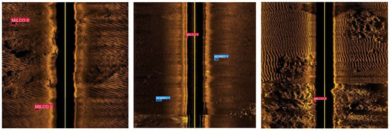
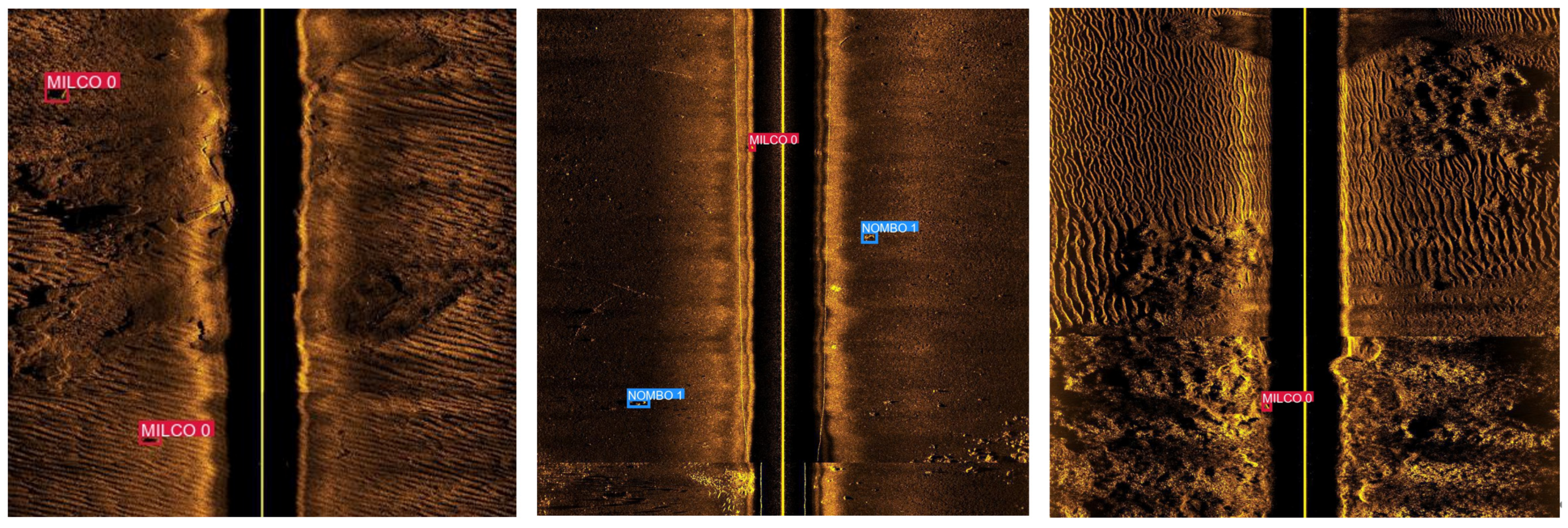
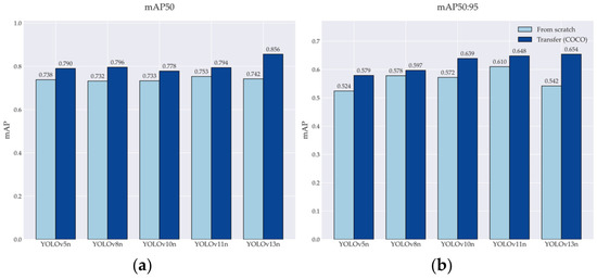
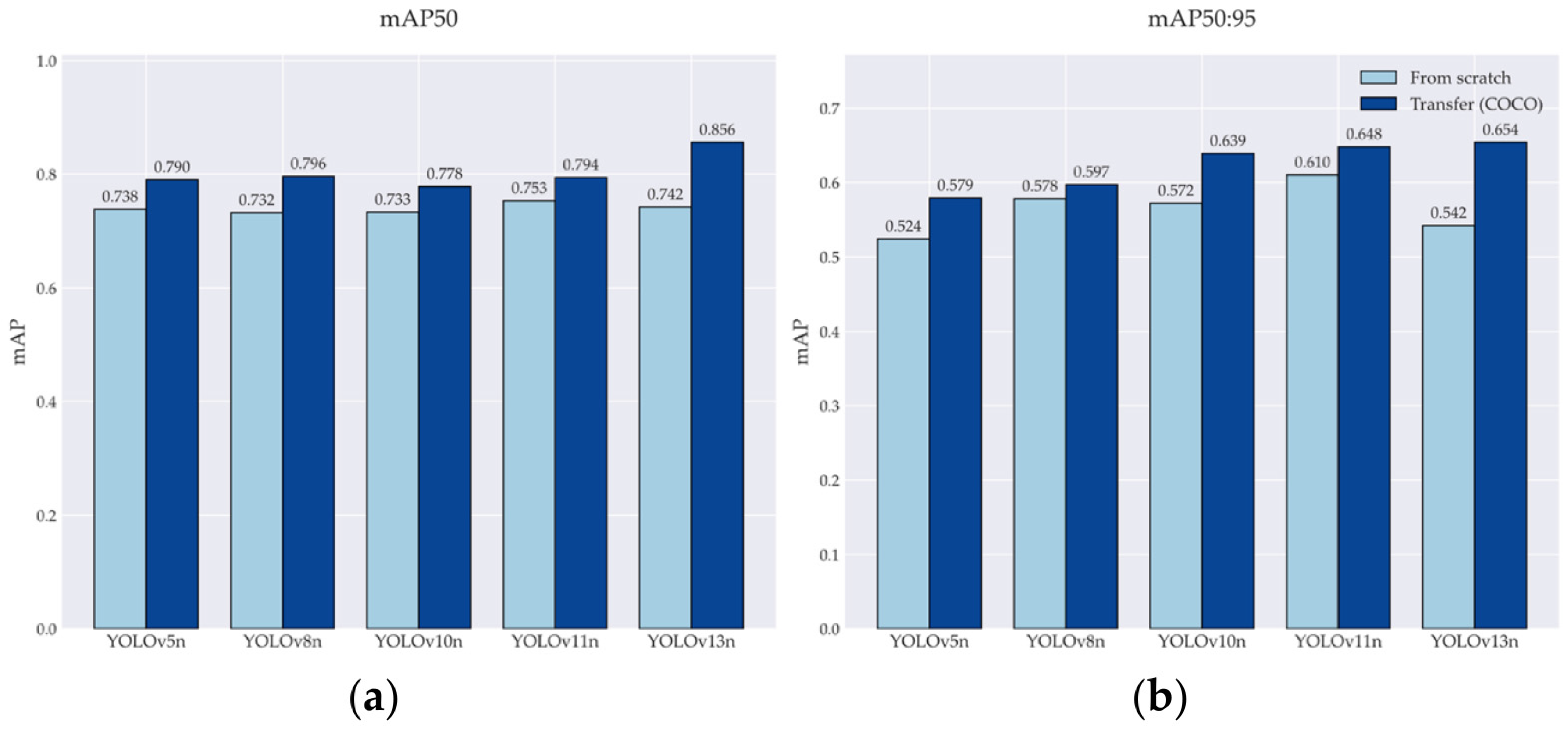
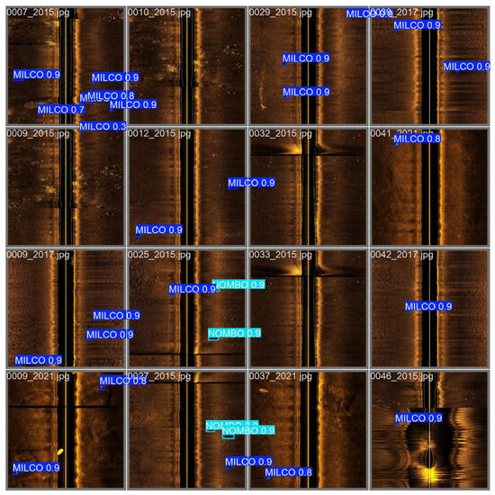
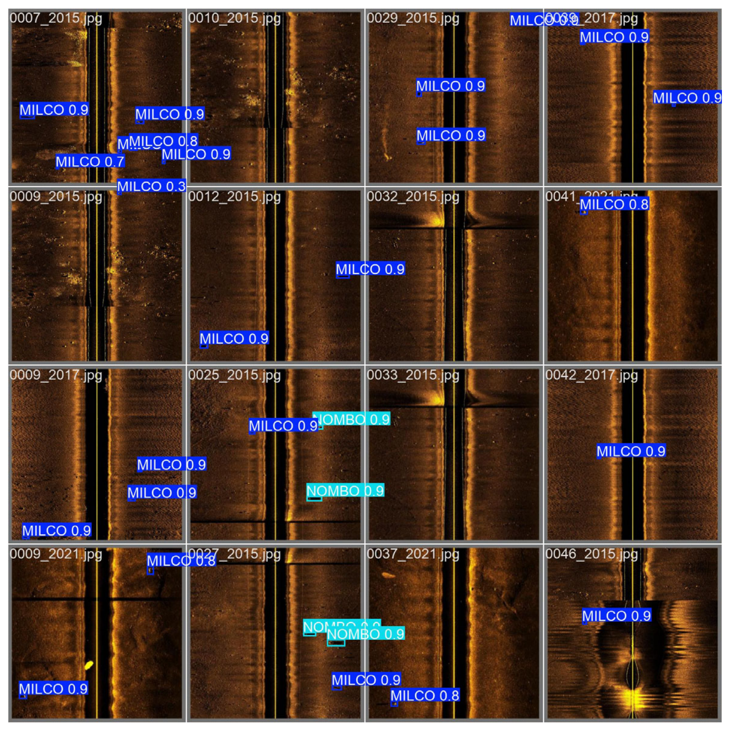
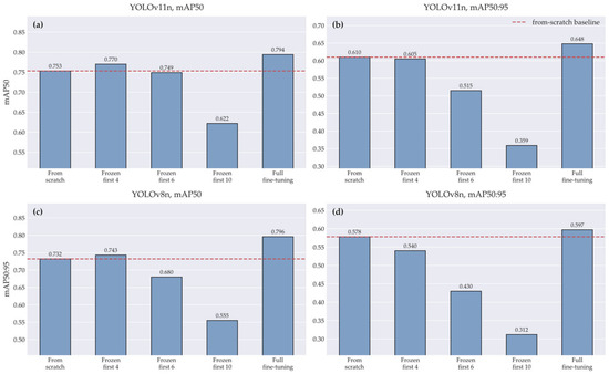
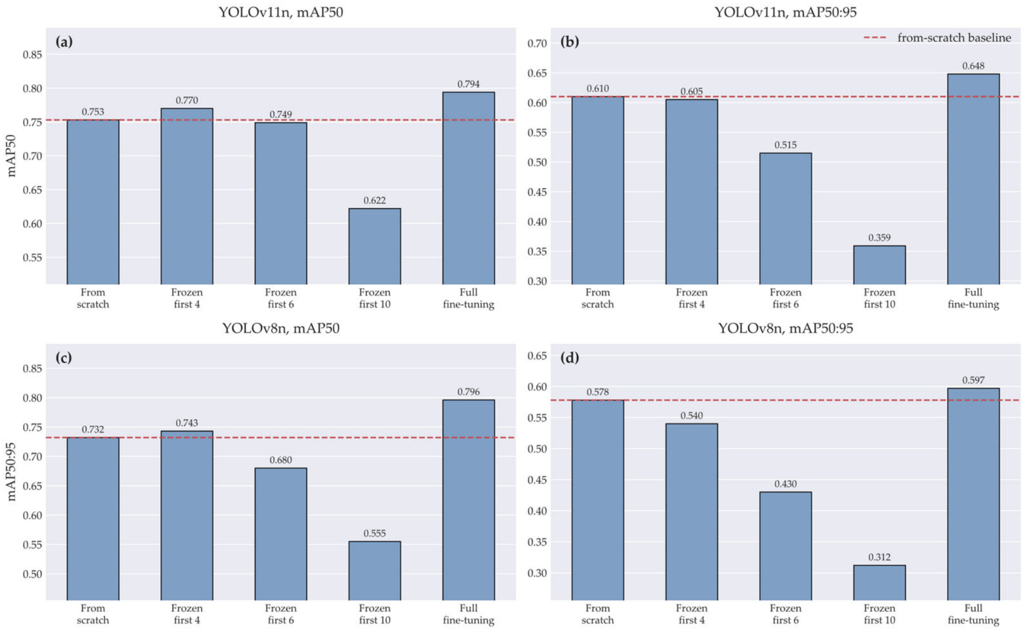

Disclaimer/Publisher’s Note: The statements, opinions and data contained in all publications are solely those of the individual author(s) and contributor(s) and not of MDPI and/or the editor(s). MDPI and/or the editor(s) disclaim responsibility for any injury to people or property resulting from any ideas, methods, instructions or products referred to in the content. |
© 2026 by the authors. Licensee MDPI, Basel, Switzerland. This article is an open access article distributed under the terms and conditions of the Creative Commons Attribution (CC BY) license.