


Abstract
The deep-sea mining industry faces opposition from those concerned about potential environmental impacts, such as the effect of sediment plumes created by mining activity. To assess the magnitude of those effects, the spatial extent of the plume, the total suspended sediment load, and the extent and thickness of the resulting sedimentation should be quantified. Here, we present a commercial-scale model of benthic plume generation from polymetallic nodule mining in the Clarion–Clipperton Zone (CCZ). This quantifies the spatial extent of the plume and resulting sedimentation after 435 days of collecting polymetallic nodules on the seafloor in the NORI-D contract area in the eastern CCZ. The model is based on a previously published hindcast model from a smaller test mining operation, scaled up to reflect commercial operations. It consists of mining a 12,624 km mining path with one collector vehicle, reflecting a realistic first phase of mining in the area. The model shows that most of the suspended sediment remains very close to the mined area, staying largely below ~8 m above the seafloor. The plume would grow to only 0.029% of the NORI-D water volume at its largest and disperses quickly over 2–5 days when operations cease. The majority of the sediment from the plume would be deposited on the mined area, with 86.7% of sediment falling within 10 m of the nearest mining path. Sedimentation thickness is dependent on the local topography and is generally 50 to 100 mm, and up to 267 mm in limited low-lying areas. Outside of the mined area, thicknesses rapidly reduce with distance from the mining path, and all thicknesses greater than 5 mm occur within 1 km of the nearest collector track. Outside of the mined area, sedimentation is characterised by very gradual sedimentation at rates on the order of microns per day or less. The results suggest that the effects of the plume and sedimentation from mining are largely limited to the mined area.
1. Introduction
The collection of polymetallic nodules from the abyssal seafloor has been discussed and explored since the 1970s, but the declining grades of terrestrial deposits, increased demand, and the need for metals for the green transition have reignited the industry [1,2,3,4]. Polymetallic nodules, which are concretions of iron and manganese oxide found in some areas of the abyssal seafloor, contain economically interesting concentrations of Mn, Cu, Ni, Co, Mo, Ti, Li, and sometimes rare earth and other elements [3,5,6]. They represent a potential untapped source of these metals without the social and environmental burden of terrestrial mining [4,5]. The Clarion–Clipperton Zone (CCZ), an area of the eastern equatorial Pacific, is estimated to contain 21.1 billion tonnes of nodules [5] and is one of the first areas to see significant advancements made towards mining [7]. However, the industry faces opposition from those with environmental concerns, largely because there is limited empirical data to quantify the spatial extent, magnitude and temporal nature of the impacts [8,9,10], especially in the context of a realistic mining operation that might continue for years.
One particular concern is the creation of sediment plumes in the water column by mining equipment: the sediment plume created near the seafloor by the seabed nodule collector vehicle (i.e., benthic plume) and the sediment plume created by returning water and sediment after separation from nodules by systems on the surface vessel (i.e., midwater plume). The benthic plume is generated mainly by sediment discharge at the rear of the nodule collector vehicle. The collector vehicle lifts nodules while entraining some portion of surface sediment [7,11], defined by the cut depth, which is the thickness of sediment removed. The nodules are separated from the sediment inside the collector vehicle, and the residual sediment–water mixture is discharged behind the vehicle, forming a sediment plume. Disturbance of the sediment surface by the collector vehicle tracks forms a weaker secondary plume [12,13]. Eastern CCZ benthic plumes are expected to be predominantly composed of fine, clay-rich siliceous ooze with coarse silt from the top seabed layer [14,15], together with nodule fragments and entrained bottom water.
Consideration of the effects of the benthic plume must begin with understanding its size and temporal nature—how far does the plume spread, over what time period, and what thicknesses of sedimentation will be produced over that area? Modelling and observation of the benthic plume have shown that most of the suspended sediment contained in the benthic plume is deposited within a few kilometres of the mining activity [15,16,17,18,19]. This is largely because the benthic plume tends to form a turbidity current or flow, which is a type of gravity-driven sediment transport where the sediment is suspended within the carrier fluid [20]. However, so far, these studies have been of limited scope in both spatial extent and duration, making it difficult to infer how the plume and sediment deposition would evolve over the timescales involved in a commercial-scale mining scenario. A quantitative, production-scale description of benthic plume behaviour is therefore a necessary foundation for credible environmental assessment. This study seeks to address that need by modelling a realistic mining scenario based on successful test mining [7] and scaled up to the proposed first phase of commercial mining in the eastern CCZ.
Here, we present a benthic plume and sedimentation model for a commercial-scale mining operation in the eastern CCZ. This model includes a 15-metre-wide collector vehicle traversing 12,624 km of seafloor during 435 operational days. A three-dimensional hydrodynamic solver is coupled to a concentration-tracking sediment-transport module, with source terms, sediment fractions, settling velocities and bed-exchange parameters inherited and adapted from the calibrated hindcast of the 2022 Nauru Ocean Resources Inc. (NORI) test mining and refined against field data [7,11]. The study aims to determine how large the plume becomes and over what time scale; where the plume travels; what suspended-sediment concentrations arise and how they are distributed; how rapidly the plume builds and then dissipates after operations cease; how sediment is redeposited relative to the collector paths; and the spatio-temporal nature of sedimentation that occurs during mining. The analysis is limited to physical dispersion and fate, not ecological acceptability or cumulative ecosystem impact. It provides exposure fields that complement emerging plume-deposition indicators, including seafloor imaging and geochemical tracers [7,12,21,22], and can inform environmental assessment, monitoring design and ecological interpretation [8,9].
2. Materials and Methods
2.1. Project Location
The model considers the planned first production phase of mining in the NORI-D exploration contract area (Figure 1). NORI-D is situated on the south-eastern margin of the CCZ, close to the Clipperton fracture zone, in the eastern equatorial Pacific. The mining area consists of a strip of relatively flat seafloor running roughly NNW–SSE through the middle of the contract area. The average water depth is approximately 4300 m, and the seafloor sediment consists of silty clay with abundant polymetallic nodules at the surface [23]. NORI-D contains a relatively flat central area, with some knolls that stand up to 700 m above the surrounding seafloor. The north and east of the contract area are characterised by NNW–SSE trending hills, and in the far south-east, there is a trough originating from the Clipperton fracture to the south. The mining area is divided into northern and southern blocks (Figure 1, Section 2.2).
Figure 1.
Location of NORI-D and the mining area in the eastern CCZ, in the eastern equatorial Pacific. The mining area is divided into the northern and southern blocks. The inset map shows the location of NORI-D (red) in the eastern CCZ and the other contract areas in light grey.
2.2. Mining System and Production Scenario
The production scenario is based on the integrated nodule collection system designed by Allseas and tested during NORI test mining in 2022 [7]. The system comprises a production vessel, a tracked collector vehicle that lifts nodules by the Coandă effect, an airlift riser, an on-board dewatering plant and a return-water discharge, which was placed at 1200 m depth in the 2022 test and at 2000 m in the production scenario (Figure 2). Of these components, only the collector vehicle generates the benthic plume, and it is the only component we model here; the midwater plume from the return-water discharge lies outside the scope of this study. The collector mobilises the upper few centimetres of sediment with the nodules, which was determined to be approximately 3.0 cm in the 2022 test [7]. It then separates the sediment from the nodules inside the vehicle. The collector then discharges the residual sediment–water mixture behind the vehicle through a diffuser designed to reduce the discharge velocity [7]. At the discharge concentrations, the fine-grained CCZ sediment begins to flocculate within minutes [15,24] (Appendix A), i.e., within the first few hundred metres behind a collector travelling at 0.30–0.35 m s−1; the mixture spreads as a near-bed density flow, although some fine material inevitably lofts [13,25]. Sediment stirred up by the tracks and by the turbulent wake of the vehicle adds a separate but minor plume contribution close to the collector path [12,13]. For the production scenario, we scaled the 6 m wide prototype (12 m long, 5 m high [7]) to a 15 m wide vehicle with ten 1.45 m Coandă heads and four 2 m wide tracks, adjusting cut depth, discharge and spill rate according to Allseas’ design calculations. The resulting seabed spill rate at the normal operating speed is 87.5 kg s−1, which the model applies as a moving source along the collector path. In reality, the collector is likely to slow down periodically, for example, to navigate obstacles or maximise nodule collection. In this way, we provide a worst-case plume scenario by applying the normal operating speed throughout the entire model.
Figure 2.
Schematic drawing of the prototype collection system drawn to scale. This depicts the system used during NORI’s 2022 test mining, upon which the scaled-up system modelled here is based. Each square is 100 × 100 m. Figure reproduced from [7] with permission.
We simulate the planned first production phase in NORI-D, in which this single collector traverses the southern and northern blocks (Figure 3). Each block is 2.4 km wide and is covered by 150 parallel passes that are spaced 16 m apart, leaving a nominal 1 m unmined strip between adjacent passes. For the purpose of the simulation, the southern block is mined first, from 15 May 2022 to 8 April 2023, including delays. It is covered by passes which are ~45 km long and arranged in a concentric pattern outwards from the centreline, adding up to 7111 km and ~243 days of mining (Table 1). After a 14 km transit of 11 h, the northern block is mined from 8 April to 29 December 2023 in ~35 km passes joined by P-turns, with the western half mined first, for 5513 km of path and ~193 days of mining. The total path is therefore 12,624 km. The collector travels at 0.35 m s−1 on straight runs, at 0.132 m s−1 in the P-turns and at 0.003–0.35 m s−1 in the concentric turns, and collects no nodules below the minimum operating speed of 0.02 m s−1, where only the track spill of Equation (10) remains. This mining pattern was chosen because long, narrow blocks minimise vessel turns. This is an idealised mining pattern: in practice, the collector will deviate around obstacles.
Figure 3.
The northern and southern blocks and the mining pattern used for each. The northern block uses parallel runs connected by P-turns, starting in the middle and moving progressively westward, before returning to the middle and progressing eastward. The southern block uses a concentric path starting in the middle and moving outward.
Table 1.
Breakdown of the model time by activity and block.
We prescribe operational delays of 146.5 h per month from day 20, weather delays of 5.5 h per month from day 5 (except September and October) and four cyclone events of 193 h starting on 5 September and 5 October of 2022 and 2023, with no sediment release during delays, so that 435 days of mining span 594 days, from 15 May 2022 to 29 December 2023, plus a final 7 days without production that allow the suspended sediment to settle (Table 1). This period spans a La Niña to El Niño transition of the Oceanic Niño Index [26]. We ran the two blocks as separate simulations and superimposed the results: by the time mining of the northern block starts, the residual southern-block plume is dilute, fully flocculated and largely settled, so it cannot drive additional density flows when the two plumes meet.
2.3. Definition of the Plume
A sediment plume is a volume of water that contains sediment particles originating from disturbed sediments. Sediment particles enter this volume from a source—in this case, mining activity—and leave it by settling on the seafloor or by dilution to a concentration below a threshold of interest, measured as total suspended solids (TSS, in mg L−1). To discuss the spatial extent of a plume, the threshold must therefore be defined with an acceptable rationale, for example, the impact on pelagic organisms. Because little data exist to set a threshold based on impact, we take a conservative approach and define the sediment plume as the volume of water within which the sediment load generated by mining is detectable above background [27]. To determine the threshold, we use background TSS data from the eastern CCZ, measured with a field-calibrated optical backscatter sensor, which provides a continuous depth profile of TSS through the water column [28,29]. The profile shows a consistent range of TSS below 1000 m depth to the seafloor and agrees with historical filtration measurements and with NORI’s McLane-pump samples [30,31,32,33]. The median of the profile is 0.03 mg L−1 and the 95th percentile 0.07 mg L−1; we therefore choose 0.07 mg L−1 as the threshold below which the plume is not detectably different from the natural range of TSS.
However, the model results represent a perturbation above the natural background; they do not include the median of 0.03 mg L−1 present naturally. We therefore report the modelled TSS that must be added to the background to reach 0.07 mg L−1, i.e., 0.04 mg L−1. Henceforth, “the plume” is the volume of water within which the modelled TSS exceeds 0.04 mg L−1, and this value is the plotting limit in all figures.
2.4. Sediment Thickness and Consolidation
The sedimentation footprint is the extent of sedimentation caused by the deposition of sediment remobilised by mining activity. Similarly to TSS levels in the plume, we compare the mining-related sedimentation to that of the natural sedimentation in the eastern CCZ. The natural sedimentation rate varies with location, benthic currents and topography, and is poorly constrained; published values for the eastern CCZ are of the order of 2–11.5 mm per thousand years [14], which corresponds to 0.016 mm (using 10 mm kyr−1) over the 600 days of modelled sedimentation. We selected a conservative plotting limit of 0.01 mm above typical background sedimentation that we believe is unlikely to be detectable in practice over the duration of the model.
Because sediment takes time to consolidate but the benthic environment experiences impacts immediately, we convert deposited mass to sediment thickness with a relatively unconsolidated dry density of 180 kg m−3, based on the measured dry density of NORI-D sediment after nine months in settling columns (Appendix A.5; Section 2.7.3). This approximates the level of sedimentation during mining and for some months afterwards; over months to years, we expect the density to increase to around 350 kg m−3, which is the in situ dry density of the natural seabed measured in geotechnical cores (Appendix A). The sediment thicknesses reported here are therefore expected to decrease over time as consolidation continues. However, this unconsolidated density of 180 kg m−3 becomes untenable as the thickness approaches the size of a sediment particle. To account for this, below 1 mm, we increase the dry density with decreasing thickness according to ρ = 350.7 exp (−0.67x), where ρ is the density in kg m−3 and x is the thickness in mm computed at 180 kg m−3; this gives 180 kg m−3 at 1 mm and reaches the consolidated values of about 350 kg m−3 at 3 µm, the d25 of the dispersed primary particles (Appendix A), below which 350 kg m−3 is used.
2.5. Modelling Framework
Collector plumes pass through a discharge phase dominated by the momentum of the discharged material and the vehicle wake, a buoyancy-driven phase in which the mixture collapses onto the seabed and spreads as a turbidity current, i.e., a gravity current driven by suspended sediment, and a passive-transport phase in which ambient currents advect and disperse the residual dilute plume over time [13,20,25]. We use “turbidity current” and “density-driven flow” interchangeably. Because a single model cannot resolve all these scales, we used a two-model approach [11]: a high-resolution near-field model (Section 2.7.4) of the discharge phase defines how sediment flux enters a far-field model that simulates the later phases over NORI-D for 600 days. We built both with DHI’s MIKE 3 Flow Model FM, coupling the hydrodynamic module (HD) dynamically to the Mud Transport module (MT) so that suspended sediment alters the fluid density and drives the density flows [34,35]. Source terms for the collector vehicle come from Allseas’s design data and the 2022 NORI test mining [7], and sediment fractions, settling and bed-exchange parameters from laboratory and field measurements on NORI-D sediment (Section 2.7 and Appendix A).
2.6. Hydrodynamic Model
2.6.1. Governing Equations and Closure
The HD module solves the three-dimensional incompressible Reynolds-averaged Navier–Stokes equations with the Boussinesq approximation [34], in its hydrostatic form for the far-field model and in its non-hydrostatic form for the near-field model only (Section 2.7.4). With z positive upwards (z = −d at the bed, z = η at the surface), the continuity and u-momentum equations read
with an analogous equation for v; the term in q is present only in the near-field model. Here, f = 2Ω sin φ is the Coriolis parameter, evaluated at the latitude of each element; q the non-hydrostatic pressure; ρ and ρ0 the local and reference densities; pA the atmospheric pressure at the surface; Fu the horizontal diffusion term; and νtv the vertical eddy viscosity. The vegetation-drag term of the module is not used. The far-field model applies the hydrostatic pressure assumption, under which q = 0; the vertical momentum equation is replaced by the hydrostatic balance, and Equations (1) and (2) reduce to the three-dimensional shallow-water equations. The near-field model (Section 2.7.4) was run with the non-hydrostatic formulation, in which the vertical momentum equation is retained and a projection method solves for q [34]. The baroclinic term (fifth on the right) allows suspended sediment to drive density flows: the model evaluates ρ at every time step from temperature and salinity and from sediment concentrations (Equation (9)). Discharges enter the discretised equations as source terms in the cell that contains them: a volume flux Q/Vi in the continuity equation and, for a source with momentum, usQ/Vi in the momentum equations, where Q is the discharge, Vi the cell volume and us the source velocity [34]; this is how the diffuser discharge is represented in the near-field model.
We close the Reynolds stresses with the Smagorinsky formulation for the horizontal eddy viscosity, in which the viscosity is proportional to the squared characteristic grid length and to the magnitude of the horizontal deformation rate [34,36], with cs = 0.28, and the standard k–ε model for the vertical eddy viscosity [34,37], with the standard constants cμ = 0.09, c1ε = 1.44, c2ε = 1.92, c3ε = 0, σk = 1.0, σε = 1.3 and σt = 0.9, the vertical eddy viscosity being νt = cμ k2/ε. Stratification enters the closure through the buoyancy production terms of the k and ε equations, Bk = νtpb and Bε = c3εcμkpb with pb = −N2/σt, where N is the Brunt–Väisälä frequency and σt the turbulent Prandtl number [34]; with c3ε = 0, the buoyancy term acts on the k equation only. Under stable stratification, the module modifies σt following the empirical expression of [38] , which damps the buoyancy production; this correction, the module default, was kept active [34,39]. The Richardson number damping of the eddy viscosity itself, νt (1 + 10 Ri)−0.5, applies only to the constant and log-law eddy-viscosity options of the module and was not used. Because the density feedback from the sediment module (Section 2.7.3) makes ρ in the buoyancy production term include the suspended sediment, the closure lets the sediment-laden near-bed layer damp turbulence [40]. The bed shear stress follows a quadratic friction law with a log-law drag coefficient Equation (3), evaluated with the velocity ub at the centre of the lowest cell (Δzb ≈ 0.5 m) and a roughness height ks = 0.05 m (cf ≈ 0.005) [34].
2.6.2. Numerical Solution
MIKE 3 FM discretises the equations with a cell-centred finite-volume method on an unstructured mesh of triangular prisms and computes the convective fluxes with the Harten–Lax–van Leer–Contact (HLLC) approximate Riemann solver [34,41]. We used the first-order explicit Euler scheme in time and first-order upwinding in space for the horizontal terms, which is diffusive but free of over- and undershoots, and the implicit scheme for the vertical terms, which removes the stability limit that the thin near-bed layers would otherwise impose [34]. The solver adapts the time step, between 10−4 and 60 s for the flow equations and between 10−3 and 75 s for the transport equations, so that the Courant number, formed from the shallow-water wave celerity plus the current speed in each horizontal direction, the time step and a characteristic length equal to twice the element area divided by its longest edge, stays below 0.8 in every cell [34]. We stored results hourly—a compromise imposed by data processing and transfer limitations. As a result, short-lived peaks in TSS occurring between model outputs may not be recorded. However, we suggest that with ~14,400 hourly snapshots, there is a very high likelihood of capturing values close to the highest TSS (i.e., the “worst case”). The remaining solver and module settings are listed in Appendix A, Table A6.
2.6.3. Domain, Adaptive Mesh, Vertical Discretisation and Bathymetry
The domain spans 359 km (N–S) by 400 km (E–W), at least 100 km beyond NORI-D on all sides, and the full water column (4.7 km) (Figure 4). A fixed mesh fine enough for the density flows would be prohibitive over this area and duration, so we used an adaptive mesh [42]: we split the path into 604 segments of ~23 km (~18 h of mining), and using Gmsh [43], meshed each with 50 m triangles within ~500 m of the segment, coarsening to 500 m at ~2 km and to 1000 m at up to 10 km from the track, and transferred the model state to the next mesh at each change of segment. This strategy halved the number of meshes from an initial 1200 to 604 and doubled the fine-mesh areas. Successive fine-mesh areas overlap by ~2 km; sensitivity tests on the overlap removed the numerical dilution at the transitions. Sixteen terrain-following sigma layers, ~1 m thick in the lowest 4 m and coarsening to 1050 m at the surface (Table 2), resolve the bottom boundary layer and the density flows, at the cost of pressure-gradient errors over steep slopes [44]. The lowest 8.4 m of the water column, which contains more than half of the plume mass (Section 3.2), is covered by six layers. The mesh therefore resolves the vertical confinement of the density current and its along-track evolution over hundreds of metres (which control the overall footprint) but not the head of the current, the Kelvin–Helmholtz billows behind it or the lateral edge of the plume, which vary over a few metres to tens of metres and are smeared over neighbouring cells by the first-order scheme. This smearing widens and dilutes the plume and is therefore conservative for the extent metrics of Section 3; the maximum concentrations reported are 50 m cell averages. The internal structure of the discharge is represented by the non-hydrostatic near-field model (Section 2.7.4). Bathymetric features wider than about two to three cells are resolved; deposits in smaller depressions are spread over the enclosing cell, conserving mass but underestimating thickness in small features.
Figure 4.
Example model mesh from the model of the northern block. An adaptive mesh follows the collector vehicle as it traverses the mining path, with a fine spacing of ~50 m around the collector vehicle’s current position.
Table 2.
Thickness of the sixteen sigma layers, from the seafloor upwards (total 4200 m at the reference depth).
We nested three bathymetric datasets (Figure 5): GEBCO_2023 (15 arc-s) [45] over the whole domain, with a constant depth of 4270 m in the unmapped margin, a 50 m EM120 multibeam grid over the exploration area, and 2 m AUV multibeam grids along the mining paths. Seamounts rising more than 300–500 m destabilised the sigma-coordinate solution, so we truncated them at 4000 m depth. This is a compromise that over-estimates deposition on their summits.
Figure 5.
Example bathymetry from the model of the northern block. The mesh has a high resolution over the mining area, which allows small features in the seafloor, like depressions and hills, to influence the progress of gravity flows. Moving outward, the mesh decreases in resolution. The area of highest resolution changes as the model progresses to stay centred over the collector vehicle.
2.6.4. Boundary Conditions, Forcing and Initial Conditions
The far-field model has four open lateral boundaries, a free surface and the seabed. On the open boundaries, we specified hourly HYCOM [46,47,48] velocities, temperature and salinity, with DTU10 tidal constituents [49] superimposed and, below the deepest HYCOM layer, the logarithmic velocity profile of Equation (4). No atmospheric forcing was applied. At the free surface, the kinematic condition applies and there is no flux of heat, salt or sediment. At the seabed, there is no flow through the bed and the bed shear stress follows the quadratic friction law of Equation (3). The k–ε model uses its standard near-wall conditions [34]. For the sediment transport Equation (5), exchange with the bed is given by the deposition and erosion fluxes of Equation (8). No sediment enters through the open boundaries. The suspended sediment concentration is set to zero on inflow, because the model represents only the effect of the sediment released by the mining activity. Sediment reaching an open boundary on outflow leaves the domain; this is the 5.5% export reported in Section 3.1. The hydrodynamic model was started from HYCOM, with the initial k and ε from Table A6. The sediment model starts with zero suspended sediment and an empty bed, so only sediment deposited by mining can later be eroded (Section 2.7.3).
Because HYCOM’s hybrid layers become several hundred metres thick in the weakly stratified abyss, its deepest layer spans the lowest ~500 m at the site, so we appended ten 1 m layers below it and scaled their velocities with a normalised logarithmic profile [50]:
where UHYCOM is the velocity of the HYCOM bottom cell, z the height above the bed, zmax = 10 m, d0 the zero-plane displacement and z0 the roughness length. We fitted the parameters (u* = 0.00354 m s−1, κ = 0.41, d0 = 0.01 m, z0 = 0.0684 m) so that the profile matches the HYCOM bottom-cell mean speed at 10 m above the bed and the mean speed measured 1 m above the bed by the long-term ADCP mooring in NORI-D, deployed during the environmental baseline campaigns that preceded the test [7]. The simulation period is representative of the long-term HYCOM record at the open boundaries.
2.7. Sediment Transport Model
2.7.1. Transport Equation and Fractions
For each sediment fraction i, the MT module solves the scalar transport equation of the flow model [34] with two additions taken from the mud-transport formulation [35]: the settling velocity wsi in the vertical advection term, and the deposition and erosion fluxes as the bed boundary condition (Equation (5)), where ci is the mass concentration, Dh and Dv the horizontal and vertical dispersion coefficients, and csiS the source term, with S being the volume flux per unit cell volume of the discharge and csi its concentration. We computed the dispersion coefficients by scaling the eddy viscosities of the flow model: Dh = 0.1 νth and Dv = 0.5 νtv [51]. The suspended sediment feeds back on the flow through the mixture density (Section 2.7.3).
We represent the discharged sediment with five fractions (Table 3). Fractions A–C flocculate and correspond to the 25th, 50th and 75th percentiles of the particle-size–settling-velocity relation measured on NORI-D sediment (Appendix A). Fraction D represents residual nodule fragments (ws = 0.102 m s−1) and fraction E fine (<5 µm) material (ws = 2 × 10⁻⁵ m s−1); we treat E as non-flocculating, consistent with the laboratory finding that flocculation of this sediment is negligible below 10 mg L−1 (Appendix A) and with the concentration dependence of flocculation kinetics [52]. Particle-size analyses of ROV water samples (n = 47) collected in the benthic plume within 150 m of the collector during the 2022 NORI test mining gave a mean <5 µm share of 5%; we assign 6.5% to fraction E, above the measured mean, so that the far-travelling fraction is over- rather than under-estimated. We assume that the test mining sediment is representative of that found in the production blocks and adopt the fractions of Table 3 (Appendix A.2).
Table 3.
Sediment fractions and settling parameters (Equations (6) and (7)). Values as entered in the production model (Appendix A, Table A1). The resulting settling velocities are shown in Appendix A, Figure A1.
2.7.2. Settling Velocity, Flocculation and Hindered Settling
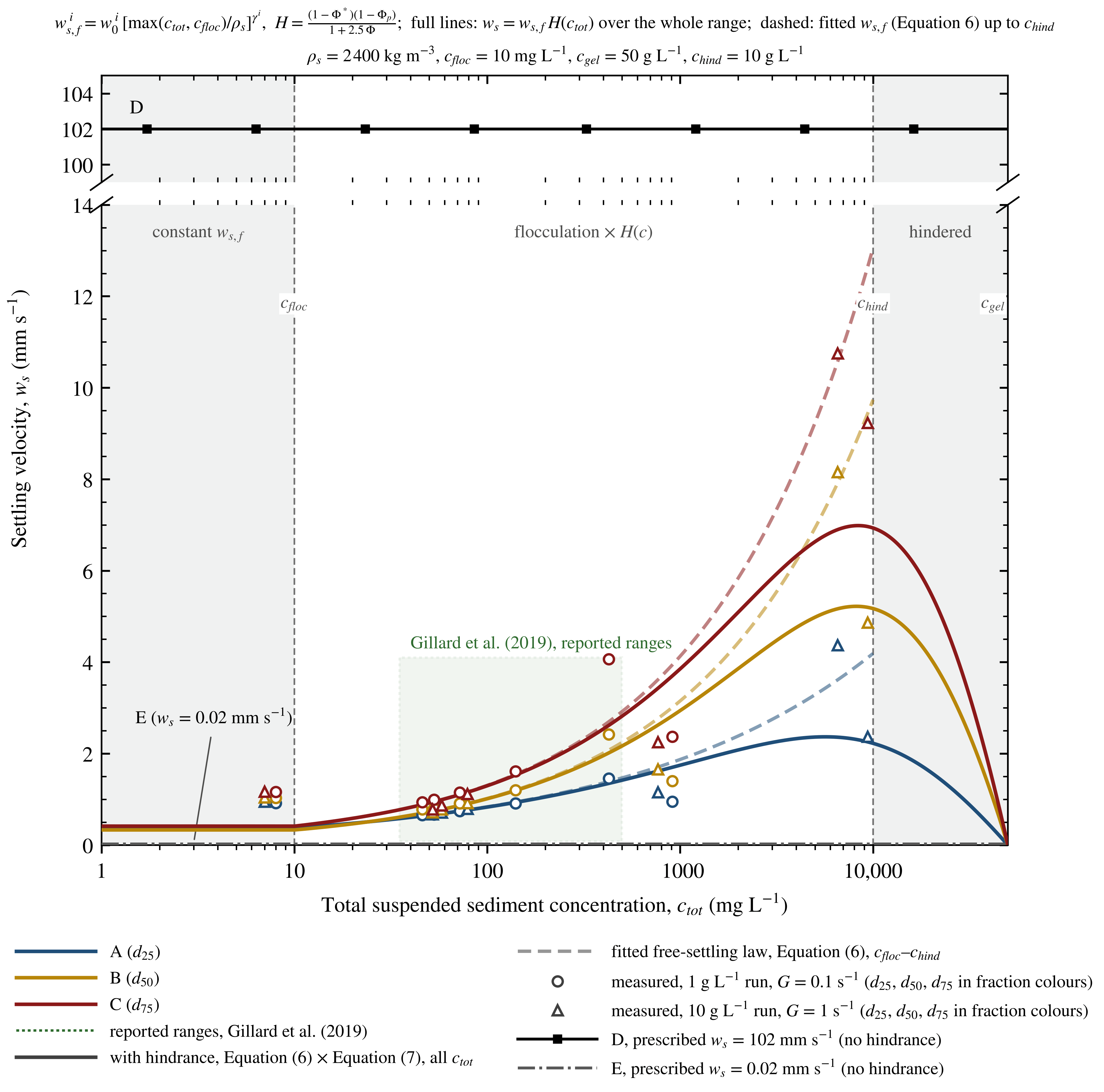
Our laboratory experiments on NORI-D sediment (Appendix A) show aggregation within 10–30 min at discharge-phase concentrations and shear rates, with settling velocities increasing with concentration, negligible flocculation below ~10 mg L−1 and hindered settling of the suspension at ~5000–10,000 mg L−1. We therefore compute the settling velocity of fractions A–C as a power law of the total volumetric concentration [35,53] (Equation (6)), with grain density ρs = 2400 kg m−3 and the flocculation threshold cfloc = 0.01 kg m−3 (below which the model holds ws at its value for cfloc):
The hindered-settling correction of [54], Equation (7), multiplies the flocculation velocity of Equation (6), which we denote ws,f, over the whole concentration range; the power constant is fixed at 1 in the module, and the settling velocity vanishes at the gelling concentration cgel = 50 kg m−3 [35,51]. Here, ϕ = ctot/cgel is the volume fraction of the flocs and ϕp = ctot/ρs that of the primary particles; the correction reduces ws,f by 7% at 1 g L−1 and by 47% at 10 g L−1, so that the settling velocity peaks at 5.6–8.4 g L−1 (Figure A1). Below cfloc, the module holds ws at its value for ctot = cfloc [51]. Figure A1 shows the resulting settling velocity of the five fractions between 1 mg L−1 and cgel, and Table A2 lists values at concentrations typical of the plume.
Equation (6) makes the settling velocity a function of concentration only. We therefore neglect the shear dependence of floc size, although laboratory studies show that CCZ clay flocculates within minutes and that floc size depends on the shear rate [15,24]. We assume that flocculation is essentially complete by the time the sediment enters the far field. Because far-field concentrations fall below the flocculation threshold near the collector, where the model holds the settling velocity at its lowest value, any further aggregation that the model ignores would increase settling and reduce the plume extent, so the assumption is conservative.
2.7.3. Bed Exchange and Deposit Properties
The MT module exchanges sediment with the bed through a deposition flux and an erosion flux that enter Equation (5) as the bed boundary condition [35]. Deposition follows [55]: the flux of fraction i to the bed is the product of its settling velocity, its near-bed concentration cb and a probability of deposition that decreases linearly from one at zero bed shear stress τb to zero at the critical shear stress for deposition τcd, as shown in Equation (8), so that nothing deposits while τb exceeds τcd. Erosion of the deposited sediment follows [56] for a soft, partly consolidated bed, as shown in Equation (8): the total erosion rate grows exponentially with the square root of the excess of τb over the critical shear stress for erosion τce, scaled by the erosion coefficient E0 and the coefficient α, and is shared among the fractions in proportion to their mass M in the bed [35]. The MT module computes τb with its logarithmic resistance law and a bed roughness of 0.01 m [35].
The erosion tests on NORI-D sediment (Appendix A.4) gave the onset of resuspension at 0.12–0.19 N m−2 for beds consolidated for at least 12 h and bounded τcd from above only. We therefore set τce = 0.10 N m−2 and τcd = 0.07 N m−2 for all fractions, both below the measured onset, so that resuspension and continued transport are over- rather than underestimated, with E0 = 5 × 10⁻⁵ kg m−2 s−1 and α = 8.3 m N−1/2 (Appendix A). The bed is a single layer that is empty at the start of the simulation, so only sediment deposited by mining can be eroded, and the natural seabed is not a sediment source; the deposit is assigned a dry density of 180 kg m−3, measured after nine months of consolidation (Appendix A.5; Section 2.4). Consolidation during the run is not modelled, and erosion stops when the suspended concentration reaches 50 kg m−3, which is the maximum concentration allowed due to erosion in the module [51].
The suspended sediment feeds back on the flow through the density: the HD module uses the mixture density from Equation (9) [35], where ρw is the water density computed from temperature and salinity and ρs = 2400 kg m−3 the grain density, so that sediment-laden water is denser than its surroundings and collapses into the turbidity currents described in Section 2.5. The module’s concentration-dependent viscosity, , reduces to the clear-water value because the base coefficient kv1 was set to 1 [35,51].
2.7.4. Source Term
Near-field model. We simulated the discharge phase with a separate, non-hydrostatic MIKE 3 FM HD–MT model (Figure 6). Its mesh has 2 m elements around the vehicle and 1 m layers; it uses higher-order schemes, a time step of 0.01–1 s and a simulated duration of 3000 s. The ten diffuser ports act as moving sources of mass and momentum in the two lowest layers: each discharges 0.265 m3 s−1, directed 17.5° downward, with velocities referenced to the ambient water. The collector travels at 0.30 m s−1 and releases 43.4 kg s−1 of sediment, the nominal production spill without overburden, divided among the five sediment classes (Table 3) in nominal shares of 30.5%, 30.5%, 30.5%, 1.0% and 7.5% for fractions A, B, C, D and E, respectively. In this run, the residual discharge momentum extends up to ~600 m behind the collector, over a width of 50–100 m, but only in the lowest 1 m layer; above it, the momentum plume extends less than 50 m behind the vehicle. This near-bed confinement is consistent with the ROV observations of the 2022 test mining, in which the benthic plume was vertically constrained and generally detectable only below 10 m above the bed [7]. Because the collector covers the 600 m over which residual discharge momentum persists in about half an hour (29–33 min at 0.35–0.30 m s−1), less than the hourly output interval, we introduce the sediment into the far-field model in the single 50 m cell that contains the collector at each time step, distributed over the six lowest layers according to the mass profile of the near-field run 50 m behind the vehicle. The far-field model then represents the spreading of this source as a density-driven flow through the mixture-density coupling of Equation (9).
Figure 6.
Example of the near-field model at the lowest layer, shown from above. The collector vehicle is the origin and travels at 0.3 m s−1, discharging 43.4 kg s−1 of sediment. The left panel shows the full plume. The right panel shows the first 200 m. The colour scale is logarithmic.
Spill rate. We compute the mass of remobilised sediment as the sum of a track spill Mtrack and a production spill Mprod:
with nt = 4 tracks of width wt = 2 m, collector speed sc, seabed dry density ρdry = 350 kg m−3 from our geotechnical cores, an effective track disturbance depth dt = 0.01 m consistent with the 0.8–1.6 cm of track penetration measured in the NORI-D Test Mining in 2022 [7], collection width wc = 15 m, the speed-dependent cut depth dc (Table 4); 0.03 m at operating speed, equal to the 3.0 cm (5th percentile 7.7 cm, 95th percentile 0.0 cm) cut depth measured in the 2022 test [7], the nodule fraction of the cut volume fn = 1.4%, the fraction of excavated sediment entering the riser fr = 2.8%, and an overburden factor R. Table A3 lists these parameters and their origin in more detail. At operating speed, the spill is 87.5 kg s−1, 36.1 kg s−1 in the P-turns and 0.1–87.5 kg s−1 in the concentric turns; below 0.02 m s−1, only the track spill remains.
Mtrack = nt sc wt ρdry dt, Mprod = sc wc ρdry dc(sc)(1 − fn)(1 − fr)R
Table 4.
Control points for the relationship between cut depth and collector speed, provided by the manufacturer of the collector vehicle, Allseas; the model interpolates linearly between them.
Overburden. The collector is expected to re-entrain part of the sediment that was deposited during earlier passes, and this process is not modelled directly. Instead, an analytical approach was used to determine an overburden resuspension factor R (Appendix A). The analytical modelling of overburden accumulation led us to select a value of R = 1.47. To determine the overburden resuspension rate, the analysis utilized a simplified numerical model and recursive algorithm that integrated single-pass base sedimentation distribution data from a physics-based sediment plume model with operational parameters such as collector cut depth, deposition density, and nominal intake height. This model iteratively calculated and redistributed sediment across successive mining passes to simulate the cumulative buildup of overburden adjacent to the tracks. By establishing a 40 mm collector intake height limit, the model yielded a base overburden resuspension rate of 49% relative to the base spill, which was adjusted down to 47% to account for the fraction of additional material captured and routed up the riser.
3. Results
3.1. Sediment Budget
Over the modelled period of 600 days, a total of 3.164 Mt of sediment was disturbed and introduced to the benthic model, comprising 2.167 Mt of production and track spill, plus 0.997 Mt of resuspended sediment. A further 0.056 Mt (~1.77%) was diverted to the riser pipe and not included in the benthic plume model. The model included a week of no production at the end to settle suspended sediment, and so only around 0.2% of the sediment was left suspended in the model mesh at the end of the simulation. Transport of sediment outside of the model domain happens semi-continuously throughout the model and accounts for 5.5% of the mass spill. This sediment export happens at very low TSS concentrations, on the order of 10−22 to 10−3 mg L−1. Of the total mass spill, including that exported from the model domain, 86.7% was deposited within 10 m of the nearest collector track, 91.4% within 1 km, and 94% within 10 km (Figure 7).
Figure 7.
Cumulative mass of sediment deposited vs. distance from the nearest collector track. A: 10 m and 86.7%, B: 1 km and 91.4%, C: 10 km and 94%.
3.2. Suspended Solids Concentration
The plume has a maximum TSS concentration of 3683 mg L−1, found directly behind the collector vehicle (Figure 8). Rapid mixing of the plume with ambient seawater, together with the settling of sediment out of suspension, quickly reduces the plume concentration as the distance from the collector vehicle increases. The highest TSS values form a lobe extending behind the collector vehicle, but are restricted in width, consistent with findings from other models [20] and observations [12]. Lateral concentration gradients are extremely high, reducing from ~1000 to 0.04 mg L−1 within 100 to 200 m (two to four mesh cells, the resolution limit of the far-field model; the near-field model gives a plume width of 50–100 m). Longitudinal concentration gradients (extending behind the collector vehicle) are less dramatic, reducing from ~1000 to 40 mg L−1 in the space of about 1.5 km. The exceedance of 0.04 mg L−1 can be expressed in time and space (Figure 9). Only 3 km2, or 0.01% of NORI-D, experiences concentrations over 0.04 mg L−1 for more than 30% of the total model run time (Figure 9A). The maximum time-exceedance of 0.04 mg L−1 is 30.2% of the run time. The influence of the prevailing current is clear, as the western side of the northern and southern blocks rarely experiences concentrations over 0.04 mg L−1. TSS concentrations significantly higher than background are found only over and directly adjacent to the mined areas (Figure 9B) due to the rapid dilution and steep lateral concentration gradients.
Figure 8.
Map showing plume concentration from an example timestep of the model. This shows the plume dispersing in a narrow area behind the collector vehicle, with extremely high lateral gradients in TSS concentration. The highest TSS levels are found in a small area just behind the collector vehicle. The plume is being swept northward and eastward by the prevailing current. Points A, B and C are referenced by later figures.
Figure 9.
(A) Contours showing the percentage of the model time spent above 0.04 mg L−1. (B) The maximum TSS concentration across all time steps, according to the hourly sampling of the model results. (C) The longest continuous duration above 0.04 mg L−1 at any time during the model.
Vertically, the sediment distribution within the plume is heavily biased towards the seafloor, with 50% of the mass of the plume across all time steps found below 6 m from the seafloor (Figure 10A), while the TSS values drop off sharply above 6 to 8 m (Figure 10B).
Figure 10.
The distribution of sediment mass and TSS in the water column across all time steps of the model. (A) The histogram shows the mass distribution in each vertical mesh layer. The black line shows the cumulative mass distribution linearly extrapolated across the vertical mesh layers. Point A: 95% at 34.4 m; Point B: 90% at 26.2 m; Point C: 50% at 6.2 m. (B) The maximum TSS encountered at any time in the model by height above the seabed. The highest TSS levels are found only below 6 to 8 m.
3.3. Transient TSS Levels
When considering the effect of the plume on the physiochemical environment, it is important to note that exposure is intermittent because TSS levels will be transient with respect to fixed points on the seafloor. To demonstrate this, three points were chosen in the southern block: directly in the collector vehicle tracks (A), ~3 km from the nearest track (B), and ~10 km away from the nearest track (C) (Figure 8). The exposure to elevated TSS was explored at those locations as a time series (Figure 11). Point A typically experiences very short durations of high TSS, generally lasting a few hours to days at a time, after which the TSS concentration quickly returns to background levels. Points B and C experience much lower TSS concentrations in general, but periods of slightly elevated TSS last longer in comparison to point A. The longest continuous duration above background TSS of 0.04 mg L−1 is approximately 960 h or 40 days, and this is restricted to a small area of less than 1 km2 to the west of the northern block (Figure 9C). Elsewhere, values of 300 h or less are more typical. This means that over the entire 600 modelled days of the mining operation, nowhere experiences continuous TSS levels above background for more than 40 days continuously. The longest durations are found close to the northern block, where the mining paths are sub-parallel to the prevailing current direction. This has concentrated the effect of the plume over a smaller area than the southern block, which is more oblique to the prevailing current.
Figure 11.
Time series of TSS at points A, B, and C indicated on Figure 8. This shows that periods of high TSS are extremely transient, lasting only a few hours or days. Further from the tracks at points B and C, only lower TSS levels are encountered.
3.4. Plume Extent
The extent of the plume is defined by the outer 0.04 mg L−1 boundary—the point where the TSS concentration in the plume returns to background levels. The extent and position of this boundary vary according to the prevailing current direction and magnitude. It most often extends in a north-eastern direction, but on occasion also extends to the north, west, and south (Figure 8, Figure 9 and Figure 12). On six occasions, the plume boundary crosses the southern border of NORI-D, and on one of these occasions, it extends up to 11 km beyond the contract area boundary. In total, the plume extends beyond the southern contract area border for 33.3 days of modelled time. In vertical extent, the plume stays close to the seafloor, hugging the terrain, with the highest TSS values seen within a few metres of the seafloor (Figure 10 and Figure 13).
Figure 12.
Snapshots from 1 h intervals of the model showing the benthic plume, coloured from 0.04 to 4.0 mg L−1, with an outer 0.04 mg L−1 contour. The four snapshots depict the plume extending to the maximum in (A) north, (B) west, (C) south and (D) east directions.
Figure 13.
Example cross-section through the plume, showing the terrain in white. The collector vehicle is travelling from left to right. The highest TSS values are seen close to the collector vehicle and the seafloor. Further from the collector vehicle, the plume shows some tendency to collect in valleys and avoid higher terrain. 50× vertical exaggeration.
The volume of the plume can be calculated at each timestep of the model using the 0.04 mg L−1 iso-surface. This shows the plume quickly grows in size over two or three days until it reaches a quasi-steady state, after which the volume stays relatively fixed until the next pause in production. This steady-state volume is on the order of 10 km3 (Figure 14, Table 5). During the pauses in production, the plume dissipates in just 2 to 5 days, until the next production period generates the plume again. Occasionally, the pauses in production are not long enough for the plume to dissipate completely between periods of mining. The maximum plume volume is 31.5 km3, which corresponds to around 0.029% of the total water volume above the seafloor of NORI-D (1.07 × 10⁵ km3). The 95th percentile plume volume is 21.9 km3, or 0.02% of the NORI-D water volume. The average residence time of the particles in the plume, indicated by dividing the mass of sediment in the plume by the rate of outflow of sediment from the plume, is usually below 10 h, with a median of 4.8 h (Figure A3). The residence time increases to ~20 h after pauses in production, when the particles left suspended are primarily of the colloidal size fraction.
Figure 14.
The volume of the plume at different TSS concentrations. Red markers indicate periods where production was occurring. (A) The full production period of the south and north blocks. (B) The selected period, highlighted in (A), showing four production periods separated by operational delays. These show that the plume reaches a maximum volume within a few days of production starting, dissipates completely within a few days in two instances, and in two instances, the plume remains until production starts again.
Table 5.
Statistics for the volume of the plume at TSS thresholds shown in Figure 14.
3.5. Sediment Thickness
The model shows that most of the sedimentation occurs on and immediately adjacent to the mined area (Figure 15). Within 10 m of the nearest collector track, sedimentation is generally between 50 and 100 mm, with a median thickness of 74.6 mm. Outside of the mined area, the sediment thickness quickly decreases (Figure 16 and Figure A4). Thicknesses of sediment greater than 5 mm are limited to within 1 km of the mined area. The greatest sedimentation depths occur in valleys and depressions, reaching up to 267 mm in depressions resolved by the 50 m mesh, and thinner sedimentation covers hills and ridges (Figure 17). Track-parallel peaks and troughs are evident in the sediment thickness (Figure 15 and Figure 17). This is likely due to the interaction between gravity-driven sediment transport and background currents, where the velocity of sediment transport, and therefore the place of deposition of that sediment, is influenced by background currents even when the mode of sediment transport is dominated by gravity-driven flow. This appears similar to current-driven effects noted in Ouillon et al. [27], where the background current was seen to influence the speed of propagation of gravity currents in different directions. In this case, background currents could be influencing the initiation of gravity current transport, thus causing deposition preferentially in one direction, or they could be causing slower propagation of the gravity flow against the prevailing background current, leading to thicker deposition over a shorter distance.
Figure 15.
The sediment footprint resulting from deposition of remobilised sediment during the benthic production model. Sediment is overwhelmingly deposited proximal to the mining area. The greatest thicknesses are found in isolated depressions and valleys. See Figure A4 for cross sections on lines a-a’ and b-b’.
Figure 16.
Violin plot showing sediment thickness grouped by distance from the centre of the nearest track. Median values are 74.6 mm (0–10 m), 13.6 mm (10 m–100 m), 1.8 mm (100 m–1 km), 0.1 mm (1–10 km) and 0.02 mm (>10 km).
Figure 17.
Two maps covering the same section of the northern block showing a comparison of the bathymetry with hill shading (A) vs. sedimentation thickness predicted by the model (B). The bathymetry includes several depression and ridge features. Comparison with the sedimentation footprint shows that greater sediment thicknesses have accumulated in the depressions, whereas thinner sediment covers the ridges. The bathymetry shown is a 1 m resolution AUV survey of the mining area, which was incorporated into the model meshes.
The geometry of the sediment footprint reflects the prevailing direction of travel of the plume, and so is primarily deposited on the mined area and to the north and north-east (Figure 15). The footprint is contained almost entirely within NORI-D, again due to the prevailing currents, as well as the geometry of the mined area, which lies closer to the central southern border than the northern or eastern boundaries. The part of the footprint outside of the contract area reaches a maximum thickness of around 0.025 mm.
3.6. Sedimentation Events
The sedimentation caused by plume deposition does not occur as a single event but as multiple sedimentation events, and the nature of these events varies with distance from the mined area (Figure 18). Proximal to the mining area, sedimentation is experienced as multiple very short but heavy events as the collector vehicle moves back and forth. The total thickness of the sedimentation comprises multiple horizons of sediment, approximately 1 to 15 mm thick. At any one point, most of the sedimentation occurs during the passes of the collector vehicle closest to the point of interest, and after that time, sedimentation is negligible in comparison. This reflects the gravity-driven flow of sediment close to the collector vehicle, and the resulting sedimentation events can be viewed as turbidites: the sediment deposit that forms from gravity-driven turbidity flow sediment transport. In contrast, for areas of the seafloor that are further from the mining area, sedimentation is experienced much more gradually. While it does occur in discrete sedimentation events, these happen as the plume is driven hydrodynamically and therefore occur semi-continuously throughout the entire mining period. During that time, individual sedimentation events occur over several days at rates of <0.001 to ~0.02 mm per day.
Figure 18.
Sedimentation over time at three points chosen from the southern mining block, as indicated on Figure 8. Note the differing Y-axis scales. Point A is on the mining tracks close to the commencement of mining, and consequently, most of the sedimentation occurs at the start, with sedimentation exceeding 15 mm d−1. At point B, sedimentation occurs gradually, at a rate of up to ~0.02 mm d−1. Point C experiences gradual sedimentation at a maximum rate of ~0.004 mm d−1. Grey lines indicate the sedimentation during each timestep of the model, blue lines are the cumulative sedimentation over the entire model time.
4. Discussion
4.1. The Plume
One of the oft-repeated claims about deep-sea mining is that sediment plumes will spread over thousands of kilometres, potentially reaching places such as Hawaii or even farther afield. Other studies have shown that sediment plumes from nodule mining activity are not likely to travel far [15,16,17,18,19]. Our model agrees with the latter finding—the relatively small maximum size of the plume precludes the possibility that it could travel far, and it does not build up over the life of a commercial mining operation. When modelling the effects of sediment plumes generated by deep-sea mining activities, it is essential to make informed decisions about the magnitude of the sediment disturbed, given that the spill rate is so closely linked to the spatial extent of the plume [57,58]. There are many parameters for the collector vehicle that need to be defined—primarily the width, the depth of disturbed sediment, and the speed of collection. The depth of disturbed sediment in particular has been reduced in recent years due to the advancement of collector vehicle technology [10,59]. The spill rate of this model, 87.5 kg s−1, is based on a real and successful mining test using modern technology [7] and on scaling up the existing collector vehicle to production size. This spill rate is ten to a thousand times less than the spill rate assumed in some other models [58,60]. The consequences are two-fold. First, the benthic sediment plume is small and transient, affecting only a small portion of the NORI-D contract area for brief periods and for only a fraction of the production time at any one place (Figure 9 and Figure 11). Second, the TSS levels of the distal plume are very low, reducing to near-background levels within hundreds of metres of the collector vehicle. The volume of water affected by high TSS levels is very small in comparison to the project area, being limited to the area immediately surrounding the mining area (Figure 7) and to heights less than 6 to 8 m above the seabed (Figure 10 and Figure 13). Fundamental to this finding is the reasoning that the outer limit of the plume must be defined by a certain threshold sediment concentration—total suspended solids in mg L−1 [27]. Here, we use a very conservative approach of defining the plume as anything above background TSS concentrations. It may be that, as further work determines the impact of different TSS concentrations, this threshold could be raised, and consequently, the predicted size of the plume defined by that threshold would reduce [8].
This model shows that the size of the plume—as quantified by its overall volume—reaches a quasi-steady state after a short period of time (Figure 14), in agreement with other mining discharge models [61]. This means that the plume does not grow indefinitely but instead is restricted in size by the balance between incoming sediment (the spill rate) and mixing, diffusion and settling processes. The quasi-steady state volume generally takes only a few days to form after the onset of production in each case. At its maximum, there remains some variation in plume size, and this can be attributed to hydrodynamic conditions that change the plume’s shape and, therefore, the surface area available for both dilution and sediment deposition. This link between the geometry of the plume and its size leads to the conclusion that the extreme thinness of the plume—typically thousands of metres long but only a few metres thick [11,12,13]—has a strong control over this maximum volume, since the flat geometry has an extremely high surface area to volume ratio. The formation of a steady-state volume is consistent with a proportional relationship between the sediment spill rate and the size of the plume [58], a relationship also seen in other types of sediment plumes such as river outflows (e.g., [62]). Further work could extend this relationship to the number of collector vehicles, given a certain spill rate, collector design, and sediment characteristics, leading to a way to predict how changing the collector design or adding more collector vehicles to a mining operation may affect the cumulative size of a mining plume. The overall volume of the plume is limited by collector technology in two ways—promotion of flocculation and turbidity current formation by diffuser design [63]—thus creating a thin plume that dissipates and settles quickly, and by reducing the cut depth and thereby limiting the amount of sediment ingested by the collector vehicle.
The volume of the plume at this steady-state condition is exceptionally small, reaching only around 0.03% of the NORI-D water volume, with a 95th percentile of 0.02%. The low volume and transient nature of the plume minimise its effect on water quality, because most of the plume’s volume has very low TSS concentrations, and exposure times are short. The highest TSS levels are only found directly behind the collector vehicle over a distance of a few hundred metres (Figure 8). This is in agreement with near-field modelling [20,58] and observations of real mining plumes (e.g., [12,27]), showing the plume extends in a narrow zone behind the collector vehicle and flows downhill as a density current. The tendency for the plume to flow into low-lying areas is in agreement with the finding that density-driven (gravity-current) processes must be represented in far-field plume predictions [27]. Furthermore, the low residence time of particles in the plume and the rapidity of plume dispersal mean that nowhere experiences TSS levels above 0.04 mg L−1 for more than ~30% of the project time, and only for ~7% as a continuous duration. Because the periods of high TSS are experienced as short pulses with periods of background level TSS in between, the area could have an opportunity to recover, at least partially, between periods of high TSS.
4.2. Sedimentation
Sedimentation resulting from the benthic plume is overwhelmingly concentrated in the mined area, with over 86.7% by mass of the deposited sediment falling within 10 m of the nearest collector path (Figure 7). This is a consequence of sediment flocculation, which increases settling velocity, and the design of the collector vehicle diffuser jets, which direct the plume downwards towards the seafloor, encouraging the formation of a density flow and therefore deposition proximal to the collector vehicle. This also caused some of the variation in thickness seen in the footprint on the mined area, with the downhill flow of the sediment-water mixture under gravity preferentially causing deposition in low-lying areas and consequently building up the thickest areas of the sediment footprint in depressions (Figure 17).
Moving outward from the mined area, sediment thicknesses quickly decrease. All thicknesses greater than 5 mm are found within 1 km of the nearest collector path. At 100–1000 m away, the median sediment thickness is only 1.8 mm (Figure 16). The analysis of sedimentation rates indicates that the sediment footprint away from the mining area is built up by gradual sedimentation, characterised by repeated but very low magnitude events, on the order of microns per day (Figure 18). Such low rates of sedimentation, although likely higher than the background sediment accumulation rate [14], are significant since we know that polymetallic nodules are often variably covered by patchy sedimentation, apparently stirred up by the feeding activity of benthic organisms [64,65]. Consequently, the environment may experience localised sediment remobilisation on an order of magnitude that the sediment accumulation rate alone does not capture. Efforts to consider the impacts of sedimentation from mining activity may want to account for these low rates and not focus solely on the total sediment thickness accumulated over the entire mining period.
The fact that most sedimentation is confined to the direct mining area suggests that sensitive areas can be protected from sedimentation by a suitably sized buffer zone. This would include environmentally sensitive areas such as seamounts, designated protected areas such as preservation reference zones, and areas external to the contract area, such as adjacent contract areas and areas of particular environmental interest (APEIs). Furthermore, the tendency of the plume to be low-lying and flow downhill naturally protects areas that stand proud of the surrounding flatter abyssal plain, such as knolls, ridges and seamounts.
5. Conclusions
Model results indicate that the plume quickly reaches a quasi-steady state where the highest TSS concentrations, up to ~3600 mg L−1, are found very close to the collector vehicle in a thin zone extending for ~500 m behind the collector vehicle, with a width of only tens of metres and a height lower than 8 m above the seafloor. Outside of this zone, TSS concentrations rapidly decrease, and consequently, the highest TSS values are only seen within metres of the mining area. The maximum volume of water affected by the plume at any one time is up to 0.029% of the total water volume within the contract area. Furthermore, the plume is highly transient, taking only 2 to 5 days to disperse completely. Sedimentation also largely occurred close to the collector vehicle: 86.7% of sediment was deposited within 10 m of the nearest collector path, and sediment thicknesses greater than 5 mm were all found within 1 km of the mining area. In the mining area, thicknesses reached a maximum of 267 mm within limited low-lying areas and were more generally 50 to 100 mm.
This commercial-scale plume and sedimentation model demonstrates that the effects of benthic sediment plumes—in terms of sedimentation and TSS increases—arising from a real mining operation are likely to be limited, both in spatial extent and in time. The areas of high TSS concentrations are small and transient, extending behind the collector vehicle in a narrow zone. Sedimentation and high TSS levels are largely limited to the mined area and directly adjacent to it. The sedimentation thickness is not homogeneous and varies with the prevailing current, topography, the mining pattern used, and the orientation of mining runs relative to the prevailing current. Areas with the highest sedimentation are likely to be valleys and troughs down-current of the collector vehicle. Even so, the data here show that exposure to the plume and sedimentation are continuous only for short periods, allowing time for a return to background conditions (TSS levels and sedimentation rates) before being affected again. Other areas uphill or up-current from the mining operations could remain relatively untouched, experiencing transient elevated TSS on rare occasions and infrequent, brief sedimentation events that are small in magnitude.
The fact that the high TSS levels and sedimentation thicknesses are limited to the mined area is consistent with the idea that sensitive areas, such as other habitat types, reference zones, or contract area boundaries, can be protected using suitably sized buffer zones [8,66]. Identifying TSS and sediment thickness tolerances for benthic organisms could help quantify suitable buffer zones and reduce the scale of the very conservative plume size and sedimentation footprint defined by the current model. Work to quantify the relationship between spill rate and the maximum size of the plume, as well as the interaction between multiple plumes, will help to predict how adding more collector vehicles could change the resulting plume size, duration, and sediment footprint. Further work could also help identify how particular current conditions, e.g., direction, speed, and current reversal conditions, could affect the size and spread of the plume.
Author Contributions
Analysis and manuscript preparation: A.P.W., J.B., L.M., P.D., F.S.F. and M.C.; Model design and conceptualization: L.M., M.C., J.B., A.B. and M.M. All authors have read and agreed to the published version of the manuscript.
Funding
This research was funded by TMC, the Metals Company Inc. (The Metals Company), through its subsidiary Nauru Ocean Resources Inc. (NORI). This is contribution TMC/NORI/D/048.
Institutional Review Board Statement
Not applicable.
Informed Consent Statement
Not applicable.
Data Availability Statement
Additional information supporting the findings of this study is available from the corresponding author upon reasonable request.
Acknowledgments
The authors gratefully acknowledge Allseas for leading the offshore test mining operations and supporting the implementation of the environmental monitoring program. We thank Anthony O’Sullivan, Claire Dalgleish, Katie Allen and Scott Wilson for project management and offshore operational support. We further thank the officers and crew of the Hidden Gem and Island Pride for their professionalism and support during offshore operations. The authors also acknowledge the scientific teams involved in offshore sampling and environmental monitoring activities that supported plume monitoring and validation. We acknowledge all the staff at DHI and the University of Gothenburg involved in the model design, fieldwork and laboratory work that supported the model parameters, as well as the staff at Allseas for operational and design parameters pertaining to the scaled-up production scenario.
Conflicts of Interest
A.P.W., J.B., F.S.F., P.D. and M.C. are employees of The Metals Company. L.M. was an employee of The Metals Company during the preparation of this manuscript. A.B. and M.M. are employees of DHI. All authors declare that the research was conducted in the absence of any commercial or financial relationships that could be construed as a potential conflict of interest.
Abbreviations
The following abbreviations are used in this manuscript:
| ADCP | Acoustic Doppler current profiler |
| APEI | Area of particular environmental interest |
| AUV | Autonomous underwater vehicle |
| BGR | Bundesanstalt für Geowissenschaften und Rohstoffe (Federal Institute for Geosciences and Natural Resources, Germany) |
| CCZ | Clarion–Clipperton Zone |
| HLLC | Harten–Lax–van Leer–Contact |
| HYCOM | Hybrid Coordinate Ocean Model |
| LISST | Laser in situ scattering and transmissometry |
| NORI | Nauru Ocean Resources Inc. |
| ROV | Remotely operated vehicle |
| SSC | Suspended sediment concentration |
| TMC | The Metals Company |
| TSS | Total suspended solids |
Appendix A. Additional Details of Model Setup
Appendix A.1. Sediment Samples and Laboratory Programme
Four sets of samples from NORI-D, all collected by TMC and analysed by contracted laboratories, underlie the sediment parameters of the model. (i) Flocculation and settling velocity were measured in 2020 by iSeaMC GmbH (Bremen) on the upper 0–15 cm of three box cores collected during the NORI-D exploration surveys that preceded the test and were shipped chilled: BC-094, BC-110 and BC-124. (ii) Erosion thresholds and deposit consolidation were measured in 2024 by the Department of Marine Sciences, University of Gothenburg (Kristineberg Center), on mixed surface sediment (0–5 cm) from box cores taken with a USNEL box corer from the monitoring vessel Island Pride during the 2022 NORI Test Mining and Monitoring Program (July–December 2022) [7], delivered together with bottom water from the site. These samples were frozen once in transit; control runs against chilled NORI-D sediment from an earlier survey showed no significant difference in aggregation, settling velocity or deposit thickness (Mann–Whitney p = 0.19–1.0). (iii) The in situ dry density of the natural seabed was measured on 181 sub-samples of the box cores of the same program, as part of its geotechnical work. (iv) The mass share of the fine fraction was derived from 47 water samples taken with ROV-mounted Niskin bottles inside the benthic plume, within 150 m of the collector, during the test-mining runs of the same program (Appendix A.2). In both laboratory campaigns, the sediment was stored at 3–4 °C, the experiments were run in cold rooms at 2–4 °C at the salinity of the site’s bottom water (34.7–35), in duplicate or triplicate, and before each experiment, the sediment was fully dispersed by pumping it for 10 min through a centrifugal pump at 3000 rpm, reproducing the shear it experiences in the collector pump.
In the 2020 campaign (sample set i), flocculation was observed in a 110 cm-diameter water-column simulator with slowly rotating inner paddles, held at 2.0 °C. Two regimes were run in triplicate: 10 g L−1 at a shear rate G ≈ 1 s−1 (near-bed flow of ~15 cm s−1, as behind the collector or during the passage of an eddy) and 1 g L−1 at G ≈ 0.1 s−1 (~4 cm s−1, ambient transport). Samples drawn at 10, 30, 60, 120, 180 and 240 min and at 24 h yielded the suspended concentration (Aqualogger 310TY turbidity meter calibrated with the same sediment, profiled over the column and logged at mid-height) and the floc-size distribution with its d25, d50, and d75 percentiles, obtained with a LISST-100X coupled with a telecentric-lens particle camera and 200–2500 particles per sample analysed with ImageJ version 1.53 [67]. The settling velocity of individual flocs was measured in a second, temperature-controlled column with 360° back-illumination and the same camera, tracking hundreds of aggregates per sample.
In the 2024 campaign (sample set ii), resuspension thresholds were measured in a 20 cm-diameter benthic erosion chamber: a bed formed from a 5 g L−1 plume was left to settle and consolidate for 24 h (and, in a second run, one month) at G = 0.1 s−1, after which the shear velocity was raised in steps of 0.1 cm s−1 every 5 min while the resuspended concentration was logged. Consolidation of fresh deposits was followed for 10 days in the simulator and 105 days in settling flasks, and continued in settling columns to 293 days. The oven-dried sub-samples of set (iii) gave an in situ dry density of 310–360 kg m−3 in the uppermost unit of the test-field box cores; over all 181 tests of the campaign, the uppermost unit ranged from 290 to 700 kg m−3 with a median of 370 kg m−3. The model adopts 350 kg m−3 (Section 2.4, Table A3).
Appendix A.2. Sediment Fractions
The discharge is represented by five fractions (Table A1): three flocculating classes (A–C) centred on the d25, d50 and d75 of the floc-size distribution, residual nodule fragments (D), and a non-flocculating fine class (E, <5 µm). The relative percentage of E (mass share in Table A1) was derived from ROV water samples (n = 47) collected with Niskin bottles from the benthic plume within 150 m of the prototype collector during the 2022 NORI Test Mining and Monitoring Program and analysed using a LISST-200X. On average, 5% of the volume was finer than 5 µm; the model conservatively assigns 6.5% to fraction E, above the measured mean, so that the far-travelling fraction is over- rather than under-estimated. A nominal 0.5% of the remaining mass was assigned to nodule fragments (D) so that their deposition could be tracked, and the rest was divided equally among A–C because the settling-velocity distribution was measured using its quartiles (Table 3 of the main text).
Table A1.
Sediment fractions of the far-field model, as entered in the settling model (Table 3 of the main text). w0 and γ refer to Equation (6).
Appendix A.3. Flocculation and Settling Velocity
Four findings of the flocculation experiments shape the settling model: (i) the dispersed sediment flocculates within tens of minutes in both shear regimes; (ii) floc settling velocity increases with concentration; (iii) flocculation was not resolved below about 10 mg L−1; and (iv) above roughly 5–10 g L−1, the flocs settle as a hindered suspension. Findings (ii) and (iii) are represented by the power law of Equation (6) with a flocculation threshold of 0.01 kg m−3, and (iv) by the hindered-settling correction of Equation (7), applied over the whole concentration range, which reduces the settling velocity progressively with concentration and to zero at the gelling concentration of 50 kg m−3 [54,68]; the hindered-settling threshold of the mud transport module is 10 kg m−3 [35,51]. The coefficients w0 and γ (Table A1) were fitted to the measured quartile settling velocities as a function of concentration, with a mean absolute error of about 15%. Figure A1 shows the resulting curves, and Table A2 gives the resulting velocities at concentrations typical of the plume. The curves are the analytical evaluation of Equations (6) and (7), in which the flocculation power law, with w0 and γ fitted to the measured settling velocities, is multiplied by the hindered-settling correction [54]. The dependence of floc size on shear rate is not represented (Section 2.7.2). Fraction E settles at a constant 2 × 10⁻⁵ m s−1 (1.7 m d−1), consistent with the 1–2 m d−1 measured in the laboratory for the unflocculated <5 µm material.
Table A2.
Settling velocity (mm s−1) of the flocculating fractions from Equations (6) and (7) with the coefficients of Table A1 (γ = 0.35/0.49/0.50). Concentration normalised by the grain density of 2400 kg m−3.
These velocities can be compared with published settling-velocity measurements on CCZ sediment [15], made on surface sediment (median diameter ≈ 20 µm) from the German (BGR) contract area in the eastern CCZ. Suspensions of 35–500 mg L−1 in artificial seawater at 1.5 °C were aggregated in roller tanks (differential settling, G ≈ 0) and in a Couette shear reactor (105–500 mg L−1; G = 2.4–10.4 s−1), with aggregation observed within 10–135 min, and the settling velocity of individual aggregates of 70–1357 µm was measured in a settling column. The velocities ranged from 7 to 355 m d−1 (0.08–4.1 mm s−1), with the study’s overall rates given of 88–102 m d−1 (1.0–1.2 mm s−1); over the same concentration range, Equations (6) and (7) give 0.6–2.8 mm s−1 for fractions A–C (Figure A1), inside the measured envelope. Three differences limit the comparison: the sediment comes from a different contract area; the concentrations tested (≤500 mg L−1) cover only the dilute end of the range fitted here (10 mg L−1 to 10 g L−1); and the same study [15] found that the shear rate, not only the concentration, controls floc size and settling velocity, with faster-settling flocs at G = 2.4 s−1, no further gain above 5.7 s−1 and a shift towards smaller aggregates at G ≈ 10 s−1, and that flocs formed at higher concentrations under differential settling settled more slowly for a given size (size-normalised velocities of 67 versus 144 m d−1 at 175 and 35 mg L−1). Equation (6) represents neither effect (Section 2.7.2). Below cfloc, the model holds the settling velocity of each fraction at its value for ctot = cfloc, w0(cfloc/ρs)γ, and the first row of Table A2 therefore applies to all concentrations up to 10 mg L−1.
Figure A1.
Settling velocity of the five sediment fractions as a function of total suspended concentration, computed analytically from Equations (6) and (7) and as applied in the model (linear velocity axis, broken to show fraction D). Symbols are the free-settling velocities of the d25, d50 and d75 floc classes derived from the floc sizes measured in the 2020 runs (sample set i; circles 1 g L−1 at G = 0.1 s−1, triangles 10 g L−1 at G = 1 s−1, sampled 10 min to 24 h after release), to which w0 and γ were fitted; they contain no hindrance by construction. Fractions A–C follow Equation (6) (dashed curves) with the coefficients of Table A1 above cfloc and are held at their cfloc value below cfloc, multiplied over the whole range by the hindered-settling correction of Equation (7) with cgel = 50 kg m−3 [54]; the correction is 7% at 1 g L−1 and 47% at 10 g L−1, so that the curves peak at 5.6–8.4 g L−1 and fall to zero at cgel. The vertical dashed lines mark the flocculation and hindered-settling thresholds of the mud transport module, cfloc and chind [35] (Figures 5.2 and 5.3). Fractions D and E settle at prescribed constant velocity to which no hindrance is applied. The dotted rectangle spans the tested concentrations and the range of floc settling velocities measured on sediment from the German contract area [15]; it is a reported range, not a validation envelope.
Appendix A.4. Erosion and Deposition Thresholds
Beds that had consolidated for 24 h or one month did not resuspend under ambient near-bed flow (~4 cm s−1, ~0.01 N m−2); loose aggregates moved as bedload from 0.019 N m−2 (6–7 cm s−1) and went into suspension from 0.047 N m−2 (11–12 cm s−1) without large-scale erosion, and in the 2020 flume tests, a complete blanket over a nodule bed withstood 15 cm s−1. Erosion of the bed itself started at 0.12–0.19 N m−2, and after more than 1 h at that stress, less than 3% of the deposit had been resuspended. The critical stress for deposition could only be bounded from above (<0.12 N m−2). The model therefore uses τce = 0.10 N m−2 for all fractions, below the measured onset, and τcd = 0.07 N m−2, within the range of literature values for fine cohesive sediment (0.05–0.1 N m−2): 0.078 N m−2 for the flume deposits of [55], as compiled in [69], and 0.08 N m−2 for the intertidal mudflat of that study, so that resuspension and continued transport are over- rather than under-estimated. Erosion of the mining deposit follows the soft-bed law of [56] with E0 = 5 × 10⁻⁵ kg m−2 s−1 and α = 8.3 m N−1/2, the eroded mass being shared among fractions in proportion to their mass in the bed [35]; the natural seabed is not erodible. Bed shear stress is computed by the sediment model with a Nikuradse roughness of 0.01 m [51].
Appendix A.5. Deposit Density
Fresh deposits form a fluid-mud layer with a dry density of 60–100 kg m−3 in the first hours, which consolidated to about 130 kg m−3 within 1–10 days and to 175 kg m−3 on average after 9 months; the model uses 180 kg m−3. Over years, the density will approach that of the natural seabed, 300–380 kg m−3 (~350 kg m−3). At the outer edge of the footprint, where the deposit is thinner than a few particle diameters, less water is entrained and the density approaches the natural value; deposited mass is converted to thickness with 180 kg m−3 above 1 mm and, below 1 mm, with a density that increases with decreasing thickness as ρ = 350.7 exp (−0.67x) (x in mm at 180 kg m−3), from 180 kg m−3 at 1 mm to the natural-bed value of about 350 kg m−3 at 3 µm, the d25 of the dispersed primary particles, and with 350 kg m−3 below 3 µm (Section 2.4).
Appendix A.6. Spill-Rate Parameters and Overburden
Table A3 lists the parameters of Equation (10). The cut-depth–speed relation (Table 4 of the main text) comes from Allseas; at the operating speed of 0.35 m s−1, it gives 0.030 m, equal to the 3.0 cm cut depth measured on the tracks of the NORI Test Mining [7]. The nodule fraction of the cut volume (1.4%) follows from the expected nodule size classes and coverage. A very conservative value was chosen to allow for uncertainty and periods where nodule cover is less than is typical. The riser fraction (fr = 2.8% of the cut volume) is Allseas’s estimate of the sediment lifted with the nodules and therefore withheld from the benthic spill. The spill rate follows the collector speed: 87.5 kg s−1 on straight runs, ~36 kg s−1 in the P-turns of the northern block (0.132 m s−1), 0.1–87.5 kg s−1 in the concentric turns of the southern block (speed rising with radius from ~0.13 to 0.35 m s−1 beyond ~1 km), and below 0.02 m s−1 only the track spill remains, and no sediment is released during delays.
Table A3.
Parameters of the spill-rate model (Equation (10)).
Overburden is sediment deposited by earlier passes that the collector re-entrains when it mines an adjacent lane. This process was not directly simulated in the far-field model and instead represented using a constant factor (R = 1.47) increase over the base production spill rate (Mprod; Equation (10)). This factor was estimated using a simple model describing repeated recycling of sediments at a fixed loss rate. A schematic of a simplified mining path is shown in Figure A2. As the collector progresses, sediment deposits on adjacent segments of the mine path. As adjacent passes are mined, this overburden sediment must be removed before nodules can be collected.
Figure A2.
Schematic of a simplified mining path. Drawing not to scale. Collector vehicle shown proceeding from left to right as indicated by the arrow.
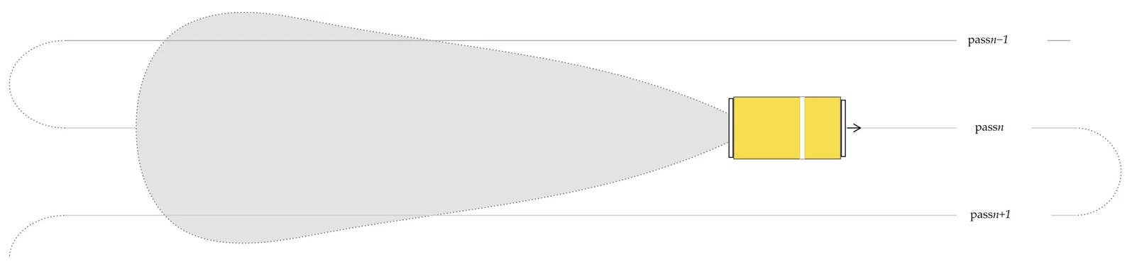
The total sediment mass to be removed by the collector after pass n, denoted Cn, can be described by the first-order recursive relationship:
where Cn−1 is the mass of existing overburden sediment that was entrained during pass n − 1 and re-deposited on the path of the nth pass; f denotes the portion of this unconsolidated overburden material that is re-suspended and subsequently re-deposited onto the path of the (n + 1)th pass; and m is the mass of material entrained while removing nodules from undisturbed (and consolidated) seabed sediment.
Cn = f ⋅ Cn−1 + m
A closed-form solution to Equation (A1) can be obtained iteratively. Assuming C0 = 0 (no overburden sedimentation before first pass):
For n = 1
X1 = f ⋅ X0 + mc = 0 + mc = mc
For n = 2
X2 = f ⋅ X1 + mc = f ⋅ mc + mc = mc ⋅ (1 + f)
For n = 3
X3 = f ⋅ X2 + mc = f ⋅ mc ⋅ (1 + f) + mc = mc ⋅ (1 + f + f2)
For n = 4
X4 = f ⋅ X3 + mc = f ⋅ mc ⋅ (1 + f + f2) + mc = mc ⋅ (1 + f + f2 + f3)
By expanding across several iterations, it can be seen that Cn has the form of a geometric series:
Cn = m ⋅ (1 + f + f2 + f3+⋯+fn−1)
Applying the formula for the sum of a geometric series yields a closed-form solution describing the mass of overburden sediment at the nth pass:
For values of f < 1, Equation (A2) converges, meaning that there is a theoretical upper limit for the amount of overburden sediment that can accumulate. Intuitively, f < 1 implies that less than 100% of the (re)suspended sediment from pass n is (re)deposited onto the path of pass n + 1. This aligns with what is expected to occur in reality, as density-flows and prevailing ocean currents will move a significant portion of the material past adjacent mine path segments before deposition occurs.
The recursive relationship for overburden mass from Equation (A1) was considered within a simple numerical framework to include cut depth, sediment density for consolidated and unconsolidated material, effective intake height of Coandă nozzles, and mechanical pushing of sediment from the suction head array at significant depths. Sediment is iteratively collected and redistributed across successive mine path segments (passes) while tracking the progressive buildup of sediment. Along a given pass, any existing overburden sediment and a fixed amount of undisturbed sediment (proportional to collector cut depth) are removed to harvest nodules. A fraction of this sediment is redistributed to adjacent passes using distribution ratios determined from sedimentation profiles extracted from the far-field model after a single pass of the collector along the mining path. The algorithm is as follows:
- Initialize and populate a vector c of length nc, with element s(i) defined as the expected sedimentation depth at multiple i of distance 𝓁 from the discharge point, and i ∈ [1,nc]. Here, 𝓁 was specified as the distance between adjacent collector paths.
- Initialize and populate a vector X(p=0) = {c,0,…,0} of length np + nc, where np represents the total number of consecutive passes (p) of the collector. The first nc elements of X are specified as the control sedimentation depths xc.
- For each pass p = {1,2,…,n − 1},
- Calculate the total depth of overburden material required to uncover nodules for the current pass as xob = min(X(p−1), h). This represents the mechanical pushing of sediment that exceeds the nominal collector intake height.
- Calculate the total mass of overburden material to be removed mob = xob ⋅ ρdep, where ρdep is the deposition density of freshly deposited sediment.
- Calculate the total mass of material to extract nodules during the current pass as mtot = mc + mob, where mc = d ⋅ ρlt is the depth of sediment removed with the nodules independent of overburden sedimentation, d is the nominal collector cut depth, and ρlt is the density of long-term consolidated sediment.
- Add new sedimentation to the adjacent ncp passes, for all i ∈ [1,nc].
This algorithm was implemented in Python using the NumPy [70] package and evaluated across parameter ranges presented in Table A4 and Table A5. Across the range of tested parameters, the model suggested that re-entrainment ranged between 20 and 80% of the base spill rate (mc), with typical values around 49% under expected operating conditions. After accounting for an expected 2% of material that would be lost to the vertical transport system, a final value of R = 1.47 was adopted in Equation (10).
Table A4.
Parameters of the overburden model.
Table A5.
Sedimentation depth control points used to define c.
Appendix A.7. Supplementary Settings
Table A6.
Far-field HD and MT MIKE model settings not given in the main text.
Appendix B. Sediment Residence Time
Average sediment residence time was obtained by dividing the mass of sediment in the plume by the outflow of sediment from the plume. The mass of sediment in the plume was obtained by adding all the masses in the model mesh cells where the TSS is equal to or greater than 0.04 mg L−1. The sediment outflow was calculated by subtracting the mass in the plume from the total sediment spill at each time step.
Figure A3.
Average residence time of particles in the benthic plume across all time steps of the model, coloured by mining block.
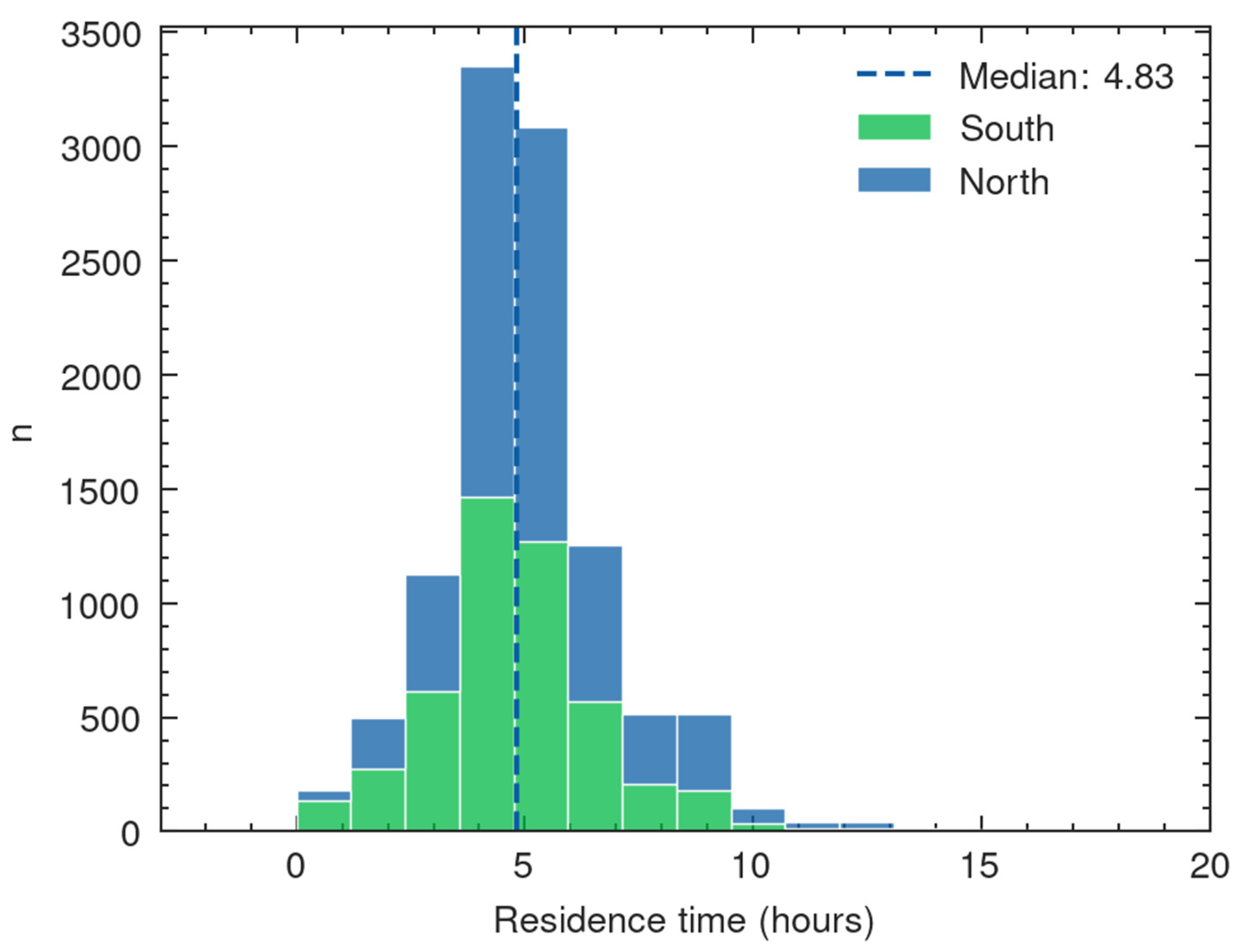
Appendix C. Sediment Thickness Cross Sections
Figure A4.
Sediment thickness cross sections along lines a-a’ and b-b’ indicated in Figure 15.
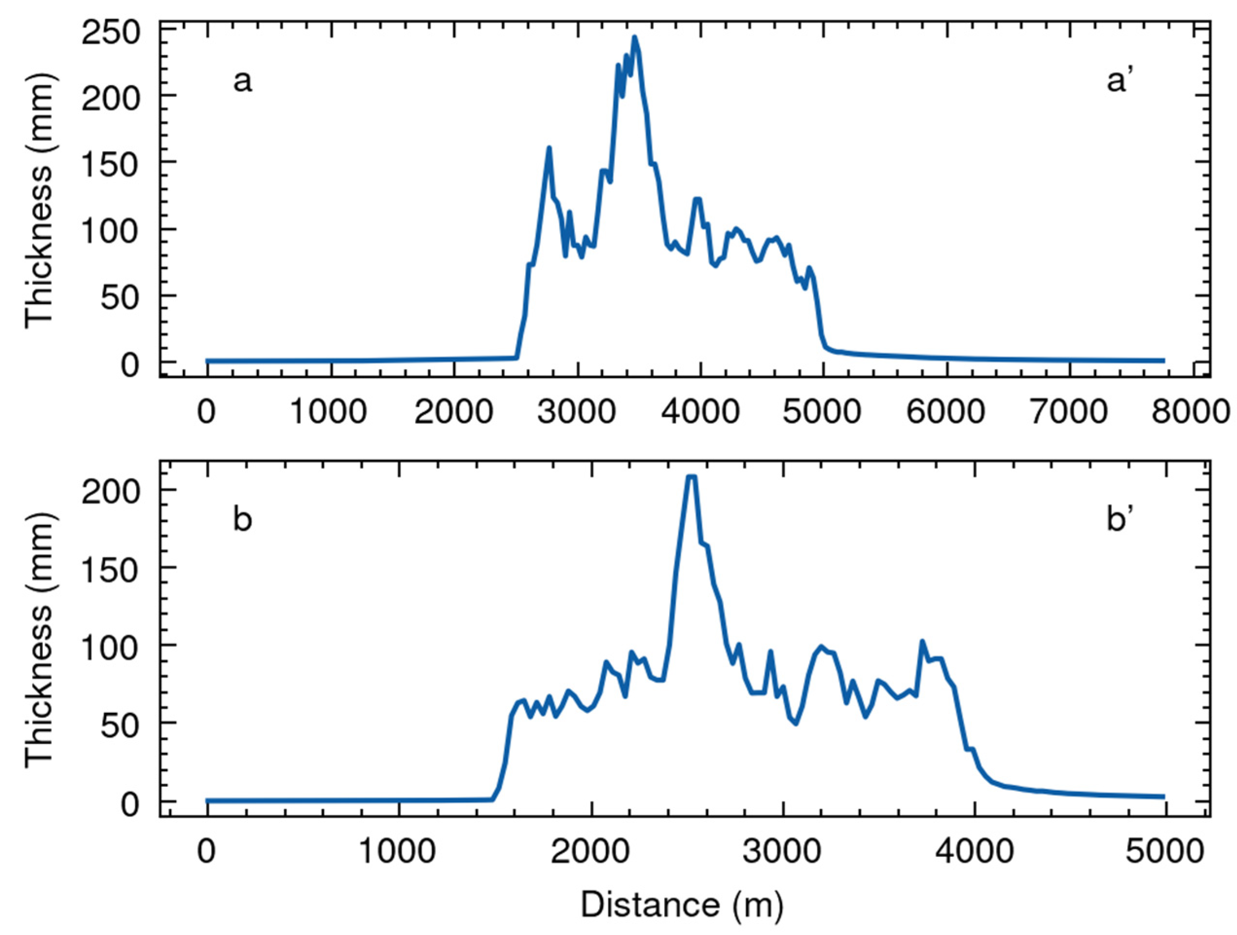
References
- Petersen, S.; Krätschell, A.; Augustin, N.; Jamieson, J.; Hein, J.R.; Hannington, M.D. News from the Seabed–Geological Characteristics and Resource Potential of Deep-Sea Mineral Resources. Mar. Policy 2016, 70, 175–187. [Google Scholar] [CrossRef] [Scilit]
- Halbach, P.; Fellerer, R. The Metallic Minerals of the Pacific Seafloor. GeoJournal 1980, 4, 407–421. [Google Scholar] [CrossRef] [Scilit]
- Hein, J.R.; Koschinsky, A.; Kuhn, T. Deep-Ocean Polymetallic Nodules as a Resource for Critical Materials. Nat. Rev. Earth Environ. 2020, 1, 158–169. [Google Scholar] [CrossRef] [Scilit]
- Paulikas, D.; Katona, S.; Ilves, E.; Ali, S.H. Deep-Sea Nodules versus Land Ores: A Comparative Systems Analysis of Mining and Processing Wastes for Battery-Metal Supply Chains. J. Ind. Ecol. 2022, 26, 2154–2177. [Google Scholar] [CrossRef] [Scilit]
- Hein, J.R.; Mizell, K.; Koschinsky, A.; Conrad, T.A. Deep-Ocean Mineral Deposits as a Source of Critical Metals for High- and Green-Technology Applications: Comparison with Land-Based Resources. Ore Geol. Rev. 2013, 51, 1–14. [Google Scholar] [CrossRef] [Scilit]
- Hein, J.R.; Koschinsky, A. Deep-Ocean Ferromanganese Crusts and Nodules. In Treatise on geochemistry; Holland, H.D., Turekian, K.K., Eds.; Elsevier: Amsterdam, The Netherlands, 2014; pp. 273–291. [Google Scholar]
- Downes, P.; Banks, A. Design and Operational Performance of Multi-Platform Environmental Monitoring During Deep-Sea Polymetallic Nodule Test Mining. J. Mar. Sci. Eng. 2026; submitted. [CrossRef] [Scilit]
- Weaver, P.P.E.; Aguzzi, J.; Boschen-Rose, R.E.; Colaço, A.; de Stigter, H.; Gollner, S.; Haeckel, M.; Hauton, C.; Helmons, R.; Jones, D.O.B.; et al. Assessing Plume Impacts Caused by Polymetallic Nodule Mining Vehicles. Mar. Policy 2022, 139, 105011. [Google Scholar] [CrossRef] [Scilit]
- Glover, A.G.; Arias, M.B.; Bribiesca-Contreras, G.; Copley, J.T.; Dahlgren, T.G.; Drazen, J.C.; Drennan, R.; Ingels, J.; Jones, D.O.B.; O’Malley, B.J.; et al. The Environmental Impacts of Deep-Sea Mining. Curr. Biol. 2026, 36, R400–R419. [Google Scholar] [CrossRef] [Scilit] [PubMed]
- Ingels, J.; Leduc, D.; Ullmann, A.; Rowden, A. Assessing Mining Impacts in the Deep Sea. Nat. Ecol. Evol. 2026, 10, 172–174. [Google Scholar] [CrossRef] [Scilit] [PubMed]
- Larsen, O.; Banks, A.; van Berkel, J.J.; Clarke, M.; Elsasser, B.; Foster, T. Monitoring and Modeling of Deep-Water Sediment Plumes from Deep-Sea Mining. In Deep-Sea Mining Management, Policy and Regulation; Sharma, R., Ed.; Springer: Berlin/Heidelberg, Germany, 2025; pp. 325–358. [Google Scholar]
- Gazis, I.-Z.; de Stigter, H.; Mohrmann, J.; Heger, K.; Diaz, M.; Gillard, B.; Baeye, M.; Veloso-Alarcón, M.E.; Purkiani, K.; Haeckel, M.; et al. Monitoring Benthic Plumes, Sediment Redeposition and Seafloor Imprints Caused by Deep-Sea Polymetallic Nodule Mining. Nat. Commun. 2025, 16, 1229. [Google Scholar] [CrossRef] [Scilit] [PubMed]
- Muñoz-Royo, C.; Ouillon, R.; El Mousadik, S.; Alford, M.H.; Peacock, T. An in Situ Study of Abyssal Turbidity-Current Sediment Plumes Generated by a Deep Seabed Polymetallic Nodule Mining Preprototype Collector Vehicle. Sci. Adv. 2022, 8, eabn1219. [Google Scholar] [CrossRef] [Scilit] [PubMed]
- Volz, J.B.; Mogollón, J.M.; Geibert, W.; Arbizu, P.M.; Koschinsky, A.; Kasten, S. Natural Spatial Variability of Depositional Conditions, Biogeochemical Processes and Element Fluxes in Sediments of the Eastern Clarion-Clipperton Zone, Pacific Ocean. Deep. Sea Res. Part I Oceanogr. Res. Pap. 2018, 140, 159–172. [Google Scholar] [CrossRef] [Scilit]
- Gillard, B.; Purkiani, K.; Chatzievangelou, D.; Vink, A.; Iversen, M.H.; Thomsen, L. Physical and Hydrodynamic Properties of Deep Sea Mining-Generated, Abyssal Sediment Plumes in the Clarion Clipperton Fracture Zone (Eastern-Central Pacific). Elem. Sci. Anthr. 2019, 7, 5. [Google Scholar] [CrossRef] [Scilit]
- Aleynik, D.; Inall, M.E.; Dale, A.; Vink, A. Impact of Remotely Generated Eddies on Plume Dispersion at Abyssal Mining Sites in the Pacific. Sci. Rep. 2017, 7, 16959. [Google Scholar] [CrossRef] [Scilit]
- Jones, D.O.B.; Kaiser, S.; Sweetman, A.K.; Smith, C.R.; Menot, L.; Vink, A.; Trueblood, D.; Greinert, J.; Billett, D.S.M.; Arbizu, P.M.; et al. Biological Responses to Disturbance from Simulated Deep-Sea Polymetallic Nodule Mining. PLoS ONE 2017, 12, e0171750. [Google Scholar] [CrossRef] [Scilit] [PubMed]
- Sharma, R.; Nagender Nath, B.; Parthiban, G.; Jai Sankar, S. Sediment Redistribution during Simulated Benthic Disturbance and Its Implications on Deep Seabed Mining. Deep. Sea Res. Part II Top. Stud. Oceanogr. 2001, 48, 3363–3380. [Google Scholar] [CrossRef] [Scilit]
- Spearman, J.; Taylor, J.; Crossouard, N.; Cooper, A.; Turnbull, M.; Manning, A.; Lee, M.; Murton, B. Measurement and Modelling of Deep Sea Sediment Plumes and Implications for Deep Sea Mining. Sci. Rep. 2020, 10, 5075. [Google Scholar] [CrossRef] [Scilit] [PubMed]
- Ouillon, R.; Kakoutas, C.; Meiburg, E.; Peacock, T. Gravity Currents from Moving Sources. J. Fluid Mech. 2021, 924, A43. [Google Scholar] [CrossRef] [Scilit]
- O’Malley, B.J.; Schwing, P.T.; Chernoch, S.K.; Larson, R.A.; Clarke, M.; Marsh, L.M.; Lough, A.J.M.; Brooks, G.R. Thorium-234 as a Tracer for Deep-Sea Mining Sediment Plume Deposition. Nat. Commun. 2025, 16, 10633. [Google Scholar] [CrossRef] [Scilit] [PubMed]
- Freitas, F.S.; Downes, P. Benthic Biogeochemical Impacts of a Deep-Sea Polymetallic Nodule Mining Test in the Southeastern Clarion-Clipperton Zone. The Metals Company, Vancouver, BC, Canada. 2026; manuscript in preparation.
- Parianos, J.; O’Sullivan, A.; Madureira, P. Geology of Parts of the Central and Eastern Clarion Clipperton Zone. J. Maps 2022, 18, 232–245. [Google Scholar] [CrossRef] [Scilit]
- Ali, W.; Kirichek, A.; Chassagne, C. Flocculation of Deep-Sea Clay from the Clarion Clipperton Fracture Zone. Appl. Ocean Res. 2024, 150, 104099. [Google Scholar] [CrossRef] [Scilit]
- Peacock, T.; Ouillon, R. The Fluid Mechanics of Deep-Sea Mining. Annu. Rev. Fluid Mech. 2023, 55, 403–430. [Google Scholar] [CrossRef] [Scilit]
- Oceanic Niño Index (ONI). Available online: https://www.cpc.ncep.noaa.gov/products/analysis_monitoring/enso/oni/v6/ (accessed on 14 August 2026).
- Ouillon, R.; Muñoz-Royo, C.; Elmousadik, S.; Peacock, T. A near Field Study of Sediment Plumes for a Pre-Prototype Nodule Collector Trial in the Abyssal Pacific Ocean. Deep. Sea Res. Part I Oceanogr. Res. Pap. 2025, 225, 104595. [Google Scholar] [CrossRef] [Scilit]
- Haalboom, S.; de Stigter, H. Suspended Particulate Matter (SPM) Filter Weights of Samples from CTD Casts During RV SONNE Cruise SO268/2 in the CCZ, NE Pacific Ocean. PANGAEA 08 March 2022. Available online: https://doi.pangaea.de/10.1594/PANGAEA.942058 (accessed on 14 August 2026).
- Haalboom, S.; Schoening, T.; Urban, P.; Gazis, I.-Z.; de Stigter, H.; Gillard, B.; Baeye, M.; Hollstein, M.; Purkiani, K.; Reichart, G.-J.; et al. Monitoring of Anthropogenic Sediment Plumes in the Clarion-Clipperton Zone, NE Equatorial Pacific Ocean. Front. Mar. Sci. 2022, 9, 882155. [Google Scholar] [CrossRef] [Scilit]
- Beer, R.M.; Dauphin, J.P.; Sholes, T.S. A Deep-Sea in-Situ Suspended Sediment Sampling System. Mar. Geol. 1974, 17, M35–M44. [Google Scholar] [CrossRef] [Scilit]
- Eittreim, S.L. Methods and Observations in the Study of Deep-Sea Suspended Particulate Matter. Geol. Soc. Lond. Spec. Publ. 1984, 15, 71–82. [Google Scholar] [CrossRef] [Scilit]
- Hobson, L.A. The Seasonal and Vertical Distribution of Suspended Particulate Matter in an Area of the Northeast Pacific Ocean. Limnol. Oceanogr. 1967, 12, 642–649. [Google Scholar] [CrossRef] [Scilit]
- Jacobs, M.B.; Ewing, M. Suspended Particulate Matter: Concentration in the Major Oceans. Science 1969, 163, 380–383. [Google Scholar] [CrossRef] [Scilit] [PubMed]
- MIKE 3 Flow Model FM-Hydrodynamic and Transport Module; DHI: Hørsholm, Denmark, 2026.
- MIKE 21 & MIKE 3 Flow Model FM-Mud Transport Module; DHI: Hørsholm, Denmark, 2026.
- Smagorinsky, J. General Circulation Experiments with the Primitive Equations: I. The Basic Experiment. Mon. Weather Rev. 1963, 91, 99–164. [Google Scholar] [CrossRef] [Scilit]
- Rodi, W. Turbulence Models and Their Application in Hydraulics: A State-of-the-Art Review/by W. Rodi., 2nd ed.; International Association for Hydraulic Research: Madrid, Spain, 1984. [Google Scholar]
- Munk, W.H.; Anderson, E.R. Notes on a theory of the thermocline. J. Mar. Res. 1948, 7, 276–295. [Google Scholar]
- MIKE 3 Flow Model FM: Hydrodynamic Module—User Guide; DHI: Hørsholm, Denmark, 2026.
- Toorman, E.A.; Bruens, A.W.; Kranenburg, C.; Winterwerp, J.C. Interaction of Suspended Cohesive Sediment and Turbulence. In Fine Sediment Dynamics in the Marine Environment; Winterwerp, J.C., Kranenburg, C., Eds.; Proceedings in Marine Science; Elsevier: Amsterdam, The Netherlands, 2002; Volume 5, pp. 7–23. [Google Scholar]
- Toro, E.F.; Spruce, M.; Speares, W. Restoration of the Contact Surface in the HLL-Riemann Solver. Shock Waves 1994, 4, 25–34. [Google Scholar] [CrossRef] [Scilit]
- Madani, M.; Foster, T.; Eden, D.; van Berkel, J.; Clarke, M. Adaptive Meshing to Enhance Sediment Plume Simulations; Western Dredging Association: Media, PA, USA, 2023. [Google Scholar]
- Geuzaine, C.; Remacle, J. Gmsh: A 3-D Finite Element Mesh Generator with Built-in Pre- and Post-processing Facilities. Numer. Methods Eng. 2009, 79, 1309–1331. [Google Scholar] [CrossRef] [Scilit]
- Haney, R.L. On the Pressure Gradient Force over Steep Topography in Sigma Coordinate Ocean Models. J. Phys. Oceanogr. 1991, 21, 610–619. [Google Scholar] [CrossRef] [Scilit]
- GEBCO Bathymetric Compilation Group. The GEBCO_2023 Grid-a Continuous Terrain Model of the Global Oceans and Land; GEBCO: Monte Carlo, Monaco, 2023. [Google Scholar]
- Bleck, R. An Oceanic General Circulation Model Framed in Hybrid Isopycnic-Cartesian Coordinates. Ocean Model. 2002, 4, 55–88. [Google Scholar] [CrossRef] [Scilit]
- Chassignet, E.P.; Hurlburt, H.E.; Smedstad, O.M.; Halliwell, G.R.; Hogan, P.J.; Wallcraft, A.J.; Baraille, R.; Bleck, R. The HYCOM (HYbrid Coordinate Ocean Model) Data Assimilative System. J. Mar. Syst. 2007, 65, 60–83. [Google Scholar] [CrossRef] [Scilit]
- Cummings, J.A. Operational Multivariate Ocean Data Assimilation. Q. J. R. Meteorol. Soc. 2005, 131, 3583–3604. [Google Scholar] [CrossRef] [Scilit]
- Cheng, Y.; Andersen, O.B. Multimission Empirical Ocean Tide Modeling for Shallow Waters and Polar Seas. J. Geophys. Res. 2011, 116, C11001. [Google Scholar] [CrossRef] [Scilit]
- Kármán, T.V. Mechanische Ähnlichkeit und Turbulenz; Weidmannsche Buchh: Göttingen, Germany, 1930. [Google Scholar]
- MIKE 21 Flow Model FM-Mud Transport Module; DHI: Hørsholm, Denmark, 2026.
- Winterwerp, J.C.; Bale, A.J.; Christie, M.C.; Dyer, K.R.; Jones, S.; Lintern, D.G.; Manning, A.J.; Roberts, W. Flocculation and Settling Velocity of Fine Sediment. In Fine Sediment Dynamics in the Marine Environment; Winterwerp, J.C., Kranenburg, C., Eds.; Proceedings in Marine Science; Elsevier: Amsterdam, The Netherlands, 2002; Volume 5, pp. 25–40. [Google Scholar]
- Burt, T.N. Field Settling Velocities of Estuary Muds. In Estuarine Cohesive Sediment Dynamics; Mehta, A.J., Ed.; Lecture Notes on Coastal and Estuarine Studies; Springer: New York, NY, USA, 1986; Volume 14, pp. 126–150. [Google Scholar]
- Winterwerp, J.C. On the Dynamics of High-Concentrated Mud Suspensions. Doctoral Thesis, Delft University of Technology, Delft, The Netherlands, 1999. [Google Scholar]
- Krone, R.B. Flume Studies of the Transport of Sediment in Estuarial Shoaling Processes; Final Report; Hydraulic Engineering Laboratory and Sanitary Engineering Research Laboratory, University of California: Berkeley, CA, USA, 1962. [Google Scholar]
- Parchure, T.M.; Mehta, A.J. Erosion of Soft Cohesive Sediment Deposits. J. Hydraul. Eng. 1985, 111, 1308–1326. [Google Scholar] [CrossRef] [Scilit]
- Muñoz-Royo, C.; Peacock, T.; Alford, M.H.; Smith, J.A.; Le Boyer, A.; Kulkarni, C.S.; Lermusiaux, P.F.J.; Haley, P.J.; Mirabito, C.; Wang, D.; et al. Extent of Impact of Deep-Sea Nodule Mining Midwater Plumes Is Influenced by Sediment Loading, Turbulence and Thresholds. Commun. Earth Environ. 2021, 2, 148. [Google Scholar] [CrossRef] [Scilit]
- Ouillon, R.; Muñoz-Royo, C.; Alford, M.H.; Peacock, T. Advection–Diffusion Settling of Deep-Sea Mining Sediment Plumes. Part 2. Collector Plumes. Flow 2022, 2, E23-1–E23-18. [Google Scholar] [CrossRef] [Scilit]
- Cheng, Y.; Dai, Y.; Zhang, Y.; Yang, C.; Liu, C. Status and Prospects of the Development of Deep-Sea Polymetallic Nodule-Collecting Technology. Sustainability 2023, 15, 4572. [Google Scholar] [CrossRef] [Scilit]
- Segschneider, J.; Sündermann, J. Simulating Large Scale Transport of Suspended Matter. J. Mar. Syst. 1998, 14, 81–97. [Google Scholar] [CrossRef] [Scilit]
- Ouillon, R.; Muñoz-Royo, C.; Alford, M.H.; Peacock, T. Advection-Diffusion-Settling of Deep-Sea Mining Sediment Plumes. Part 1: Midwater Plumes. Flow 2022, 2, E22-1–E22-19. [Google Scholar] [CrossRef] [Scilit]
- Pawlowicz, R.; Di Costanzo, R.; Halverson, M.; Devred, E.; Johannessen, S. Advection, Surface Area, and Sediment Load of the Fraser River Plume Under Variable Wind and River Forcing. Atmosphere-Ocean 2017, 55, 293–313. [Google Scholar] [CrossRef] [Scilit]
- Ali, W.; Enthoven, D.; Kirichek, A.; Chassagne, C.; Helmons, R. Effect of Flocculation on Turbidity Currents. Front. Earth Sci. 2022, 10, 1014170. [Google Scholar] [CrossRef] [Scilit]
- Paul, A.Z. Deep-Sea Bottom Photographs Show That Benthic Organisms Remove Sediment Cover from Manganese Nodules. Nature 1976, 263, 50–51. [Google Scholar] [CrossRef] [Scilit]
- Subin Raj, V.B.; Sarun Lal, M.A.; Gowri, R.S.; Ramesh, S.; Ramesh, N.R.; Ramesh, R.; Deepak, V.; Vadivelan, A.; Ramadass, G.A. Assessment of Polymetallic Nodules in the Central Indian Ocean Basin: Factors Influencing Distribution Patterns through High-resolution Autonomous Underwater Vehicle (AUV) Survey. Geo-Mar. Lett. 2025, 45, 7. [Google Scholar] [CrossRef] [Scilit]
- Wedding, L.M.; Friedlander, A.M.; Kittinger, J.N.; Watling, L.; Gaines, S.D.; Bennett, M.; Hardy, S.M.; Smith, C.R. From Principles to Practice: A Spatial Approach to Systematic Conservation Planning in the Deep Sea. Proc. R. Soc. B Biol. Sci. 2013, 280, 20131684. [Google Scholar] [CrossRef] [Scilit] [PubMed]
- Schneider, C.A.; Rasband, W.S.; Eliceiri, K.W. NIH Image to ImageJ: 25 Years of Image Analysis. Nat. Methods 2012, 9, 671–675. [Google Scholar] [CrossRef] [Scilit] [PubMed]
- Winterwerp, J.C. On the Flocculation and Settling Velocity of Estuarine Mud. Cont. Shelf Res. 2002, 22, 1339–1360. [Google Scholar] [CrossRef] [Scilit]
- Shi, B.; Wang, Y.P.; Yang, Y.; Li, M.; Li, P.; Ni, W.; Gao, J. Determination of Critical Shear Stresses for Erosion and Deposition Based on In Situ Measurements of Currents and Waves over an Intertidal Mudflat. J. Coast. Res. 2015, 316, 1344–1356. [Google Scholar] [CrossRef] [Scilit]
- Harris, C.R.; Millman, K.J.; van der Walt, S.J.; Gommers, R.; Virtanen, P.; Cournapeau, D.; Wieser, E.; Taylor, J.; Berg, S.; Smith, N.J.; et al. Array Programming with NumPy. Nature 2020, 585, 357–362. [Google Scholar] [CrossRef] [Scilit] [PubMed]
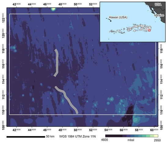
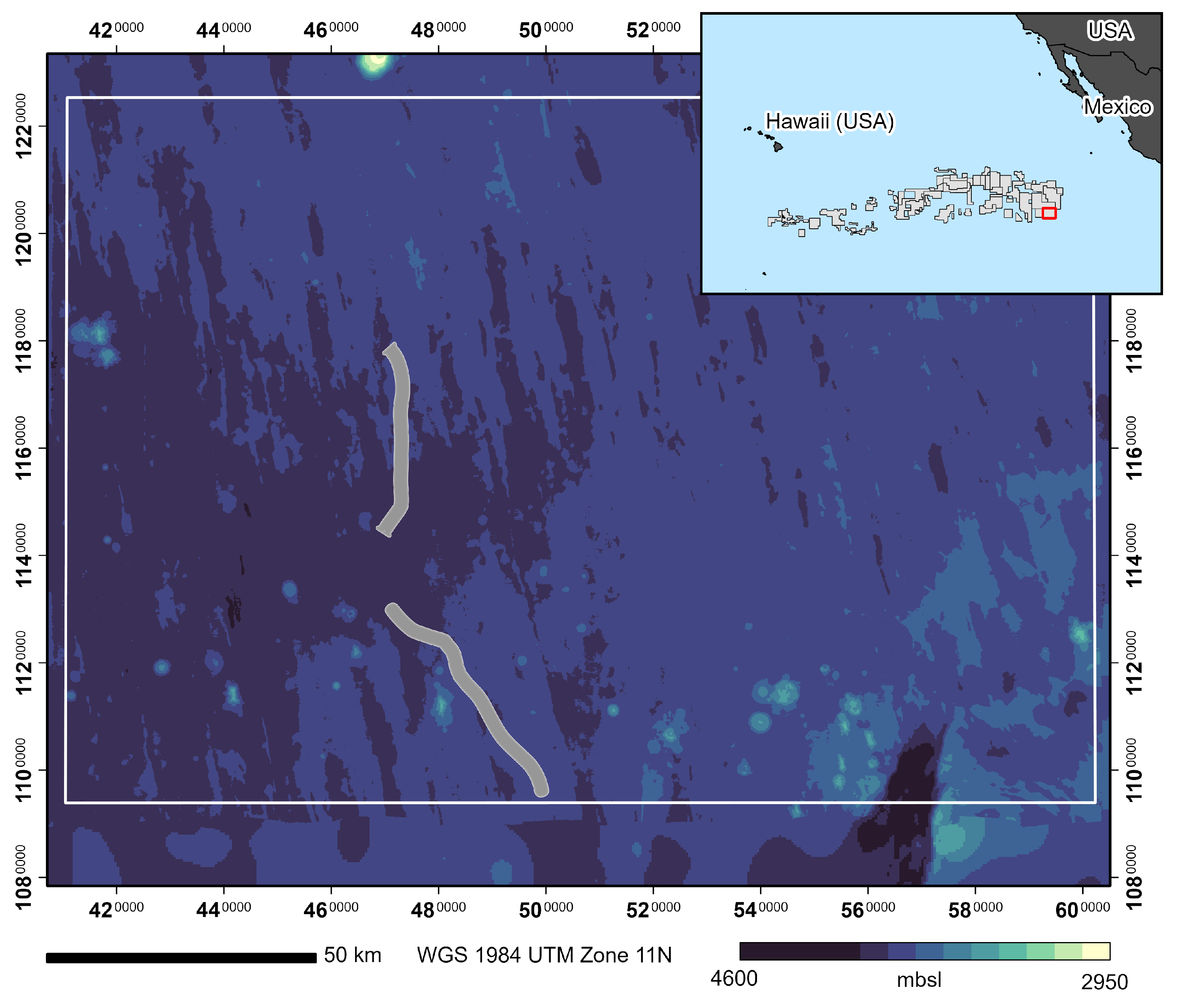
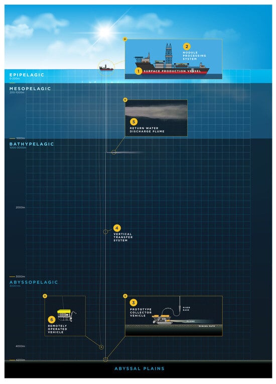
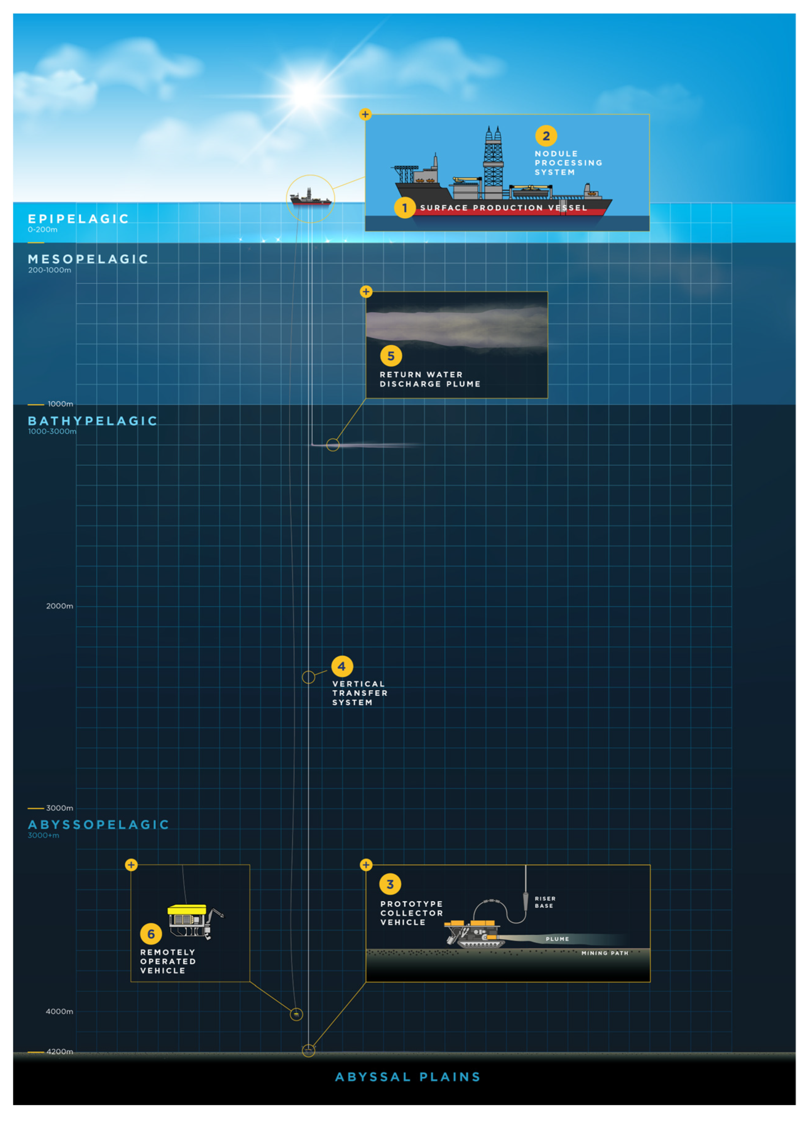
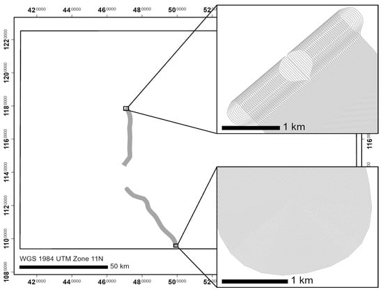
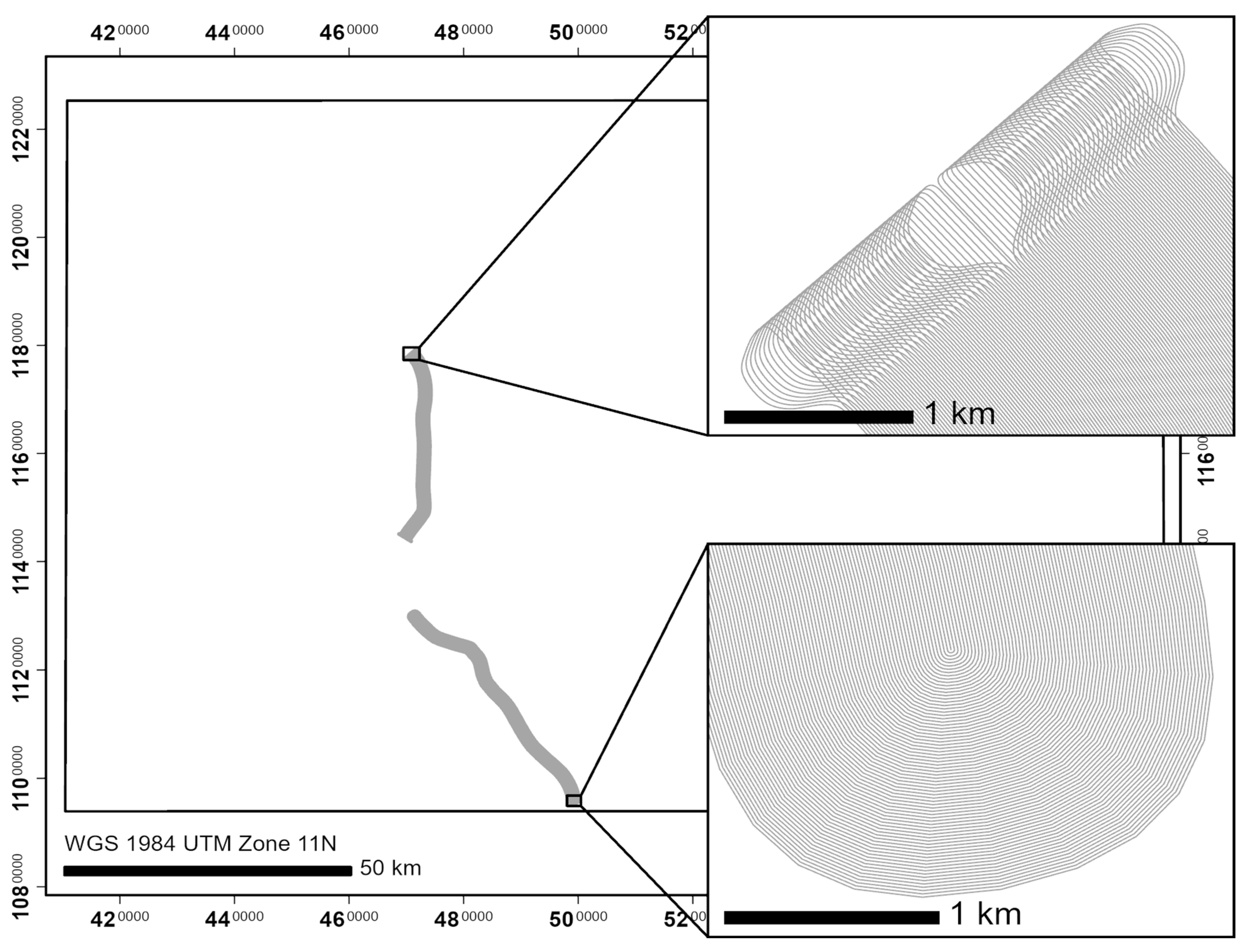
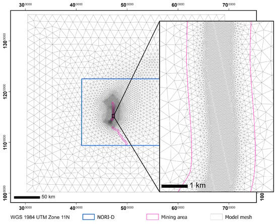
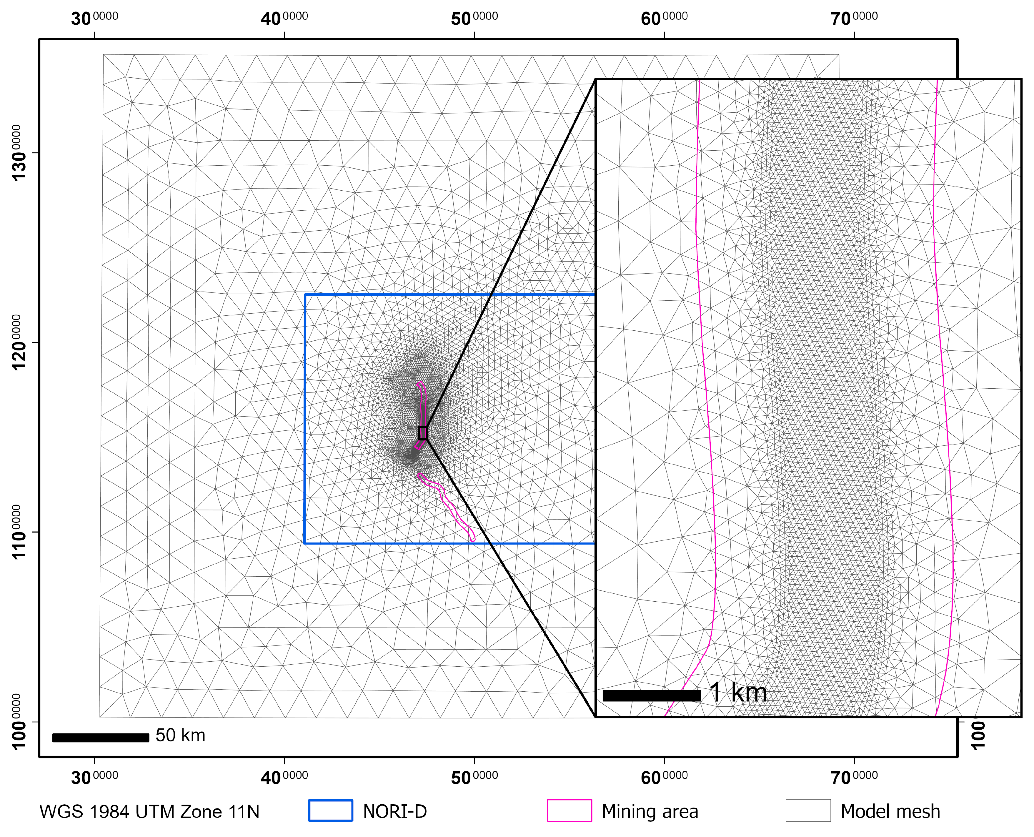
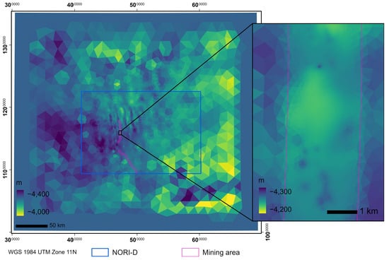
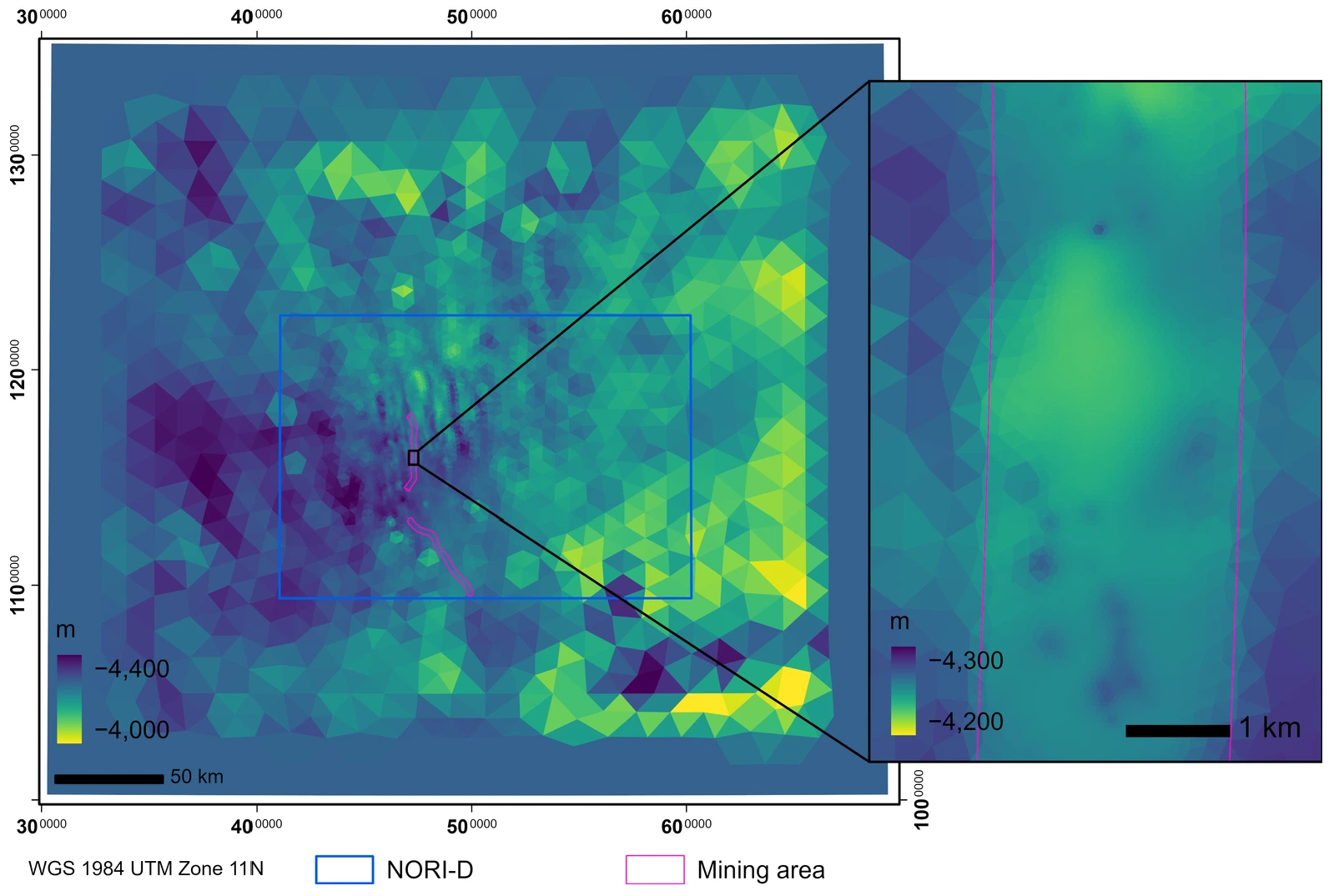
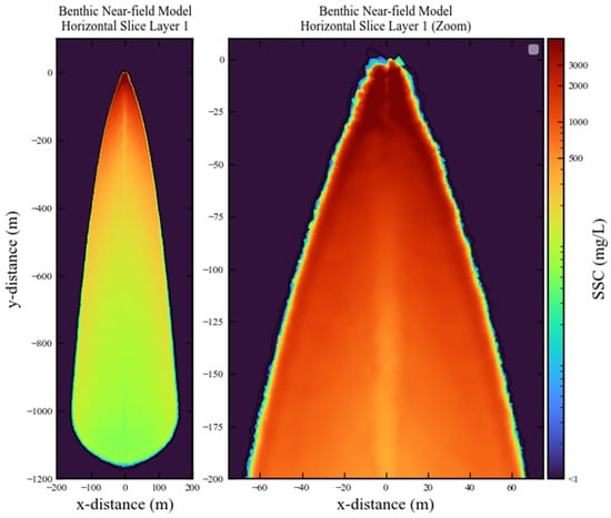
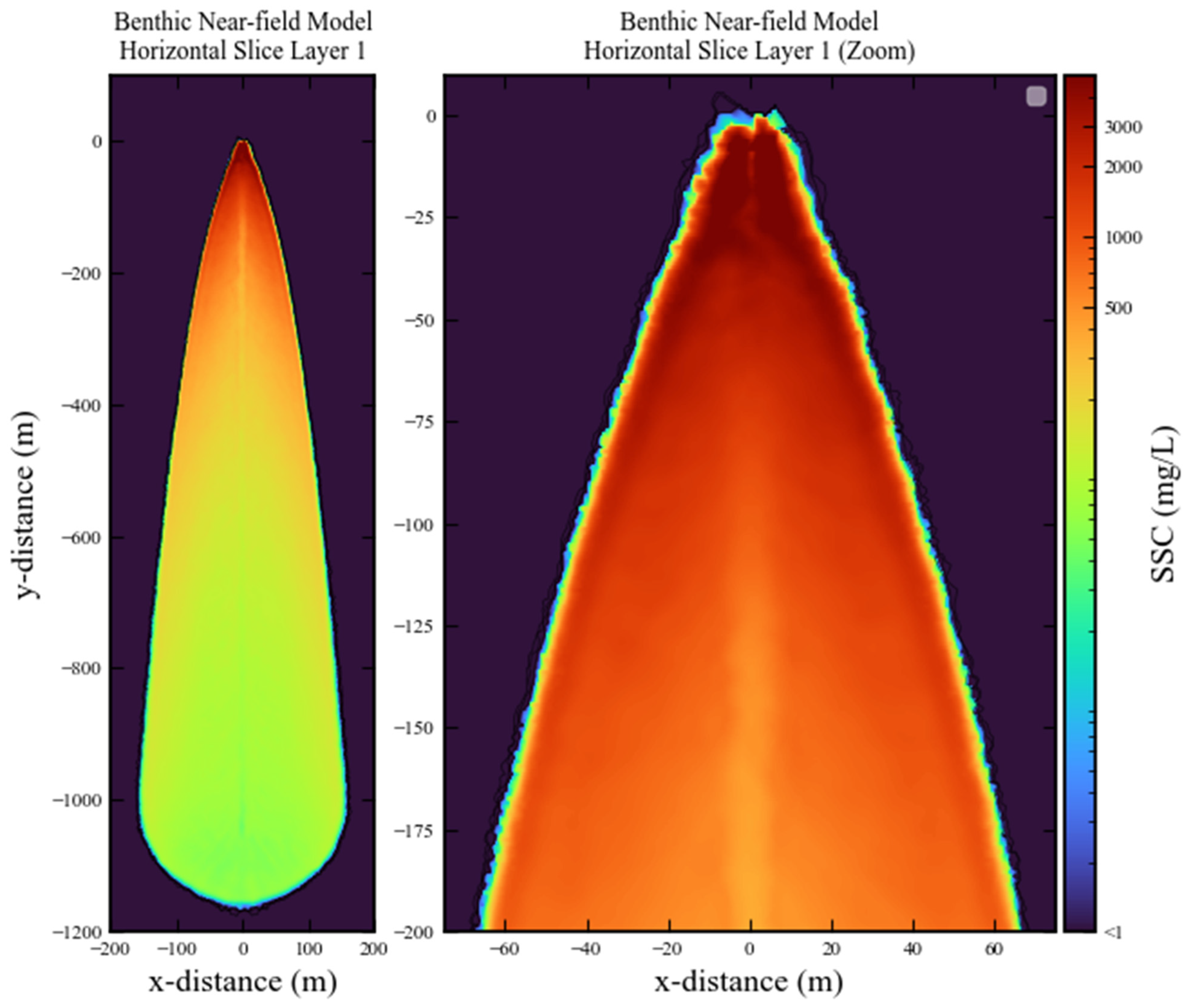
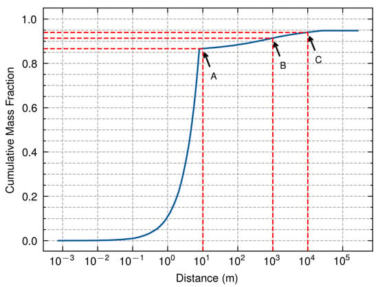
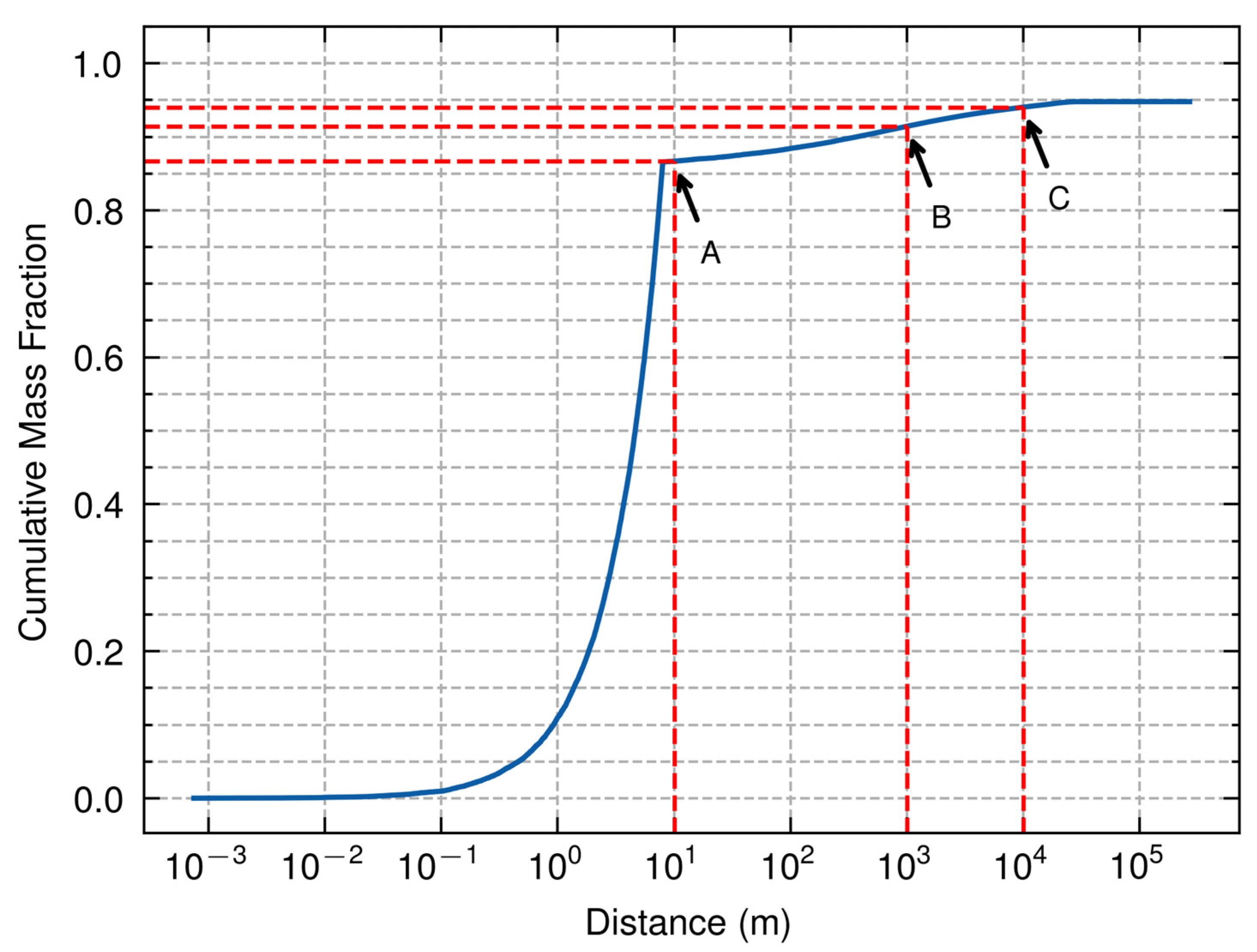
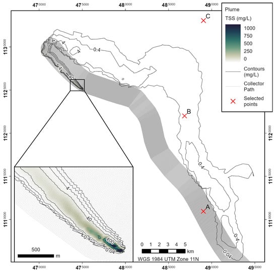
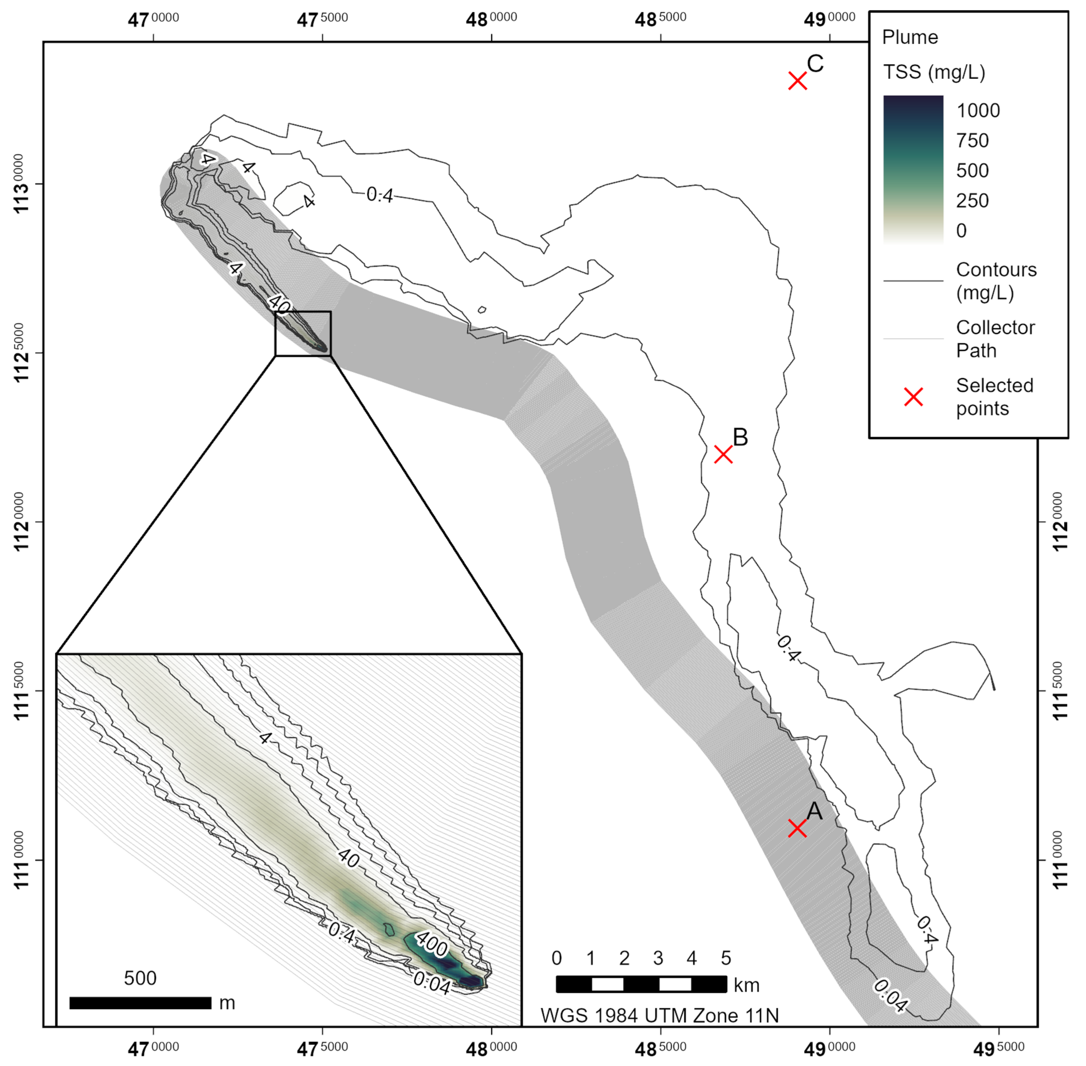
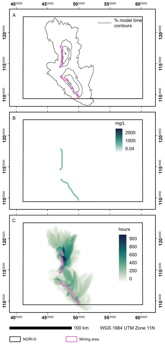
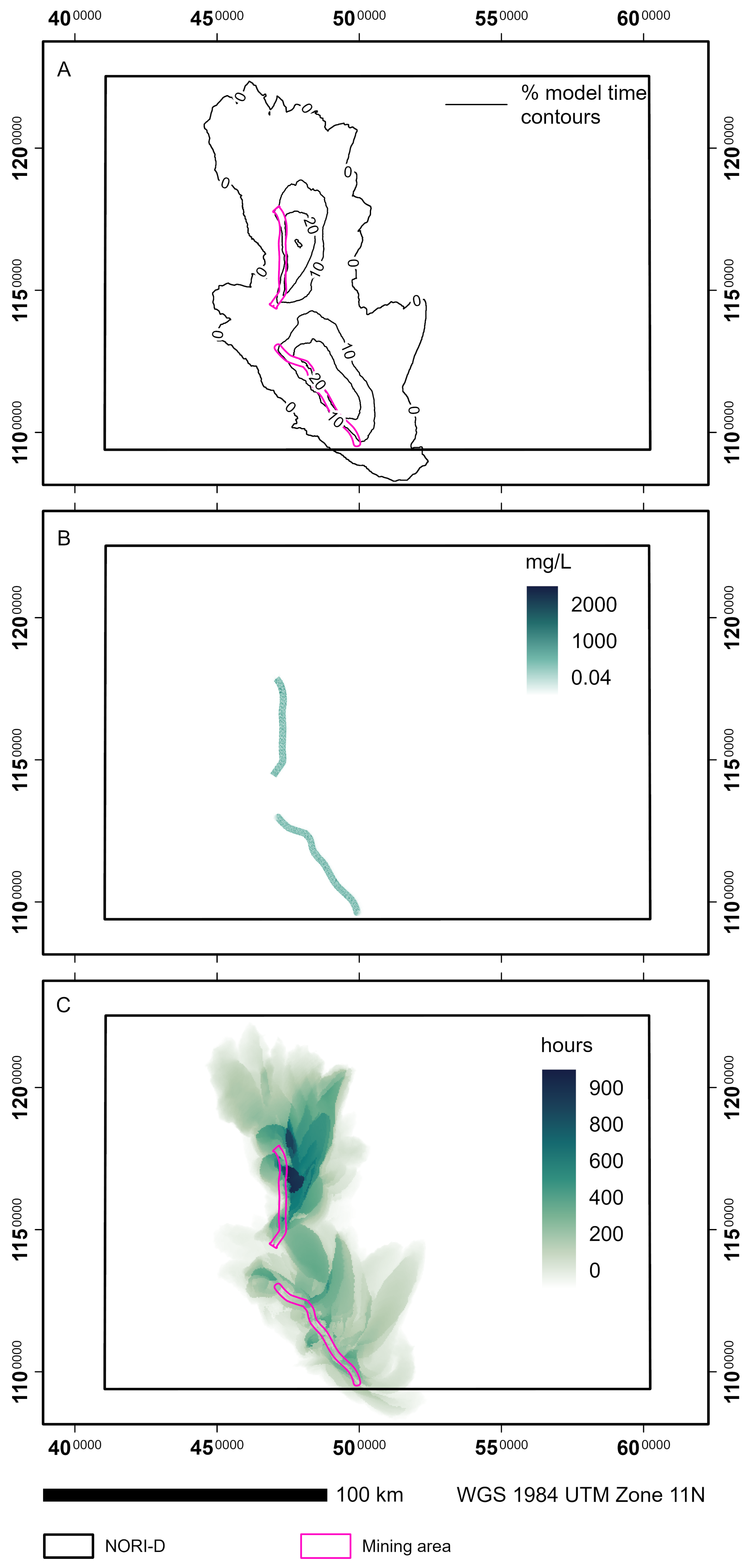
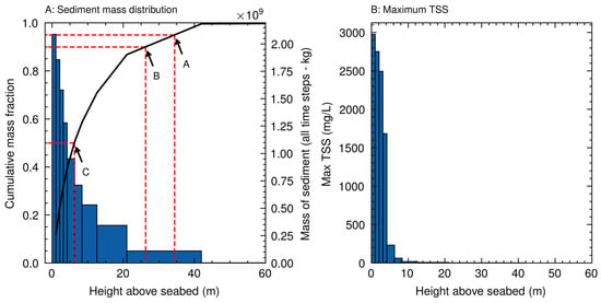
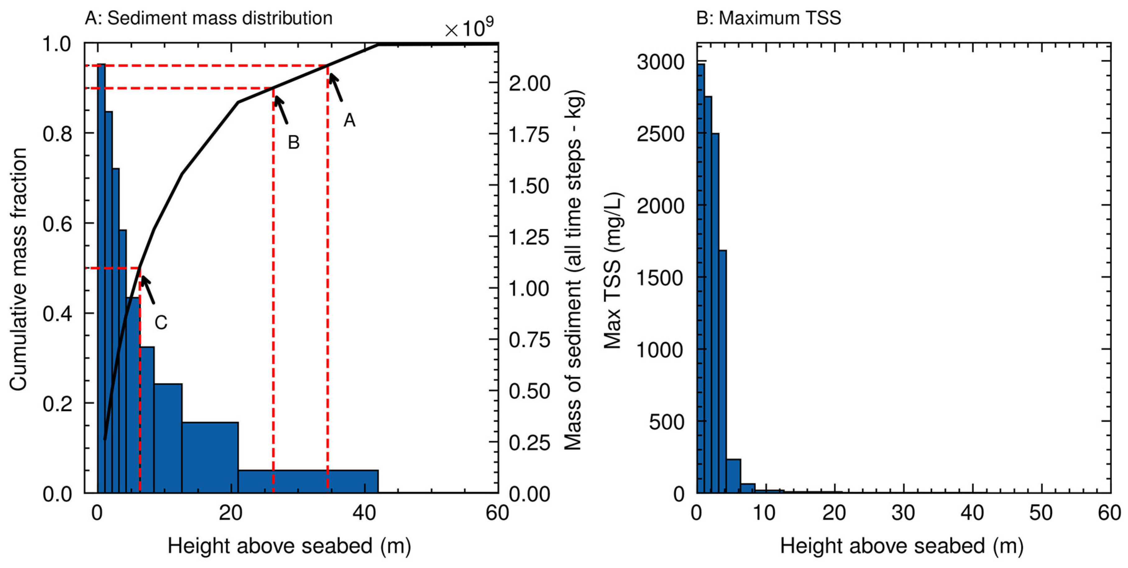
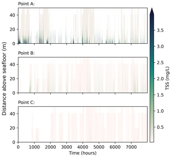
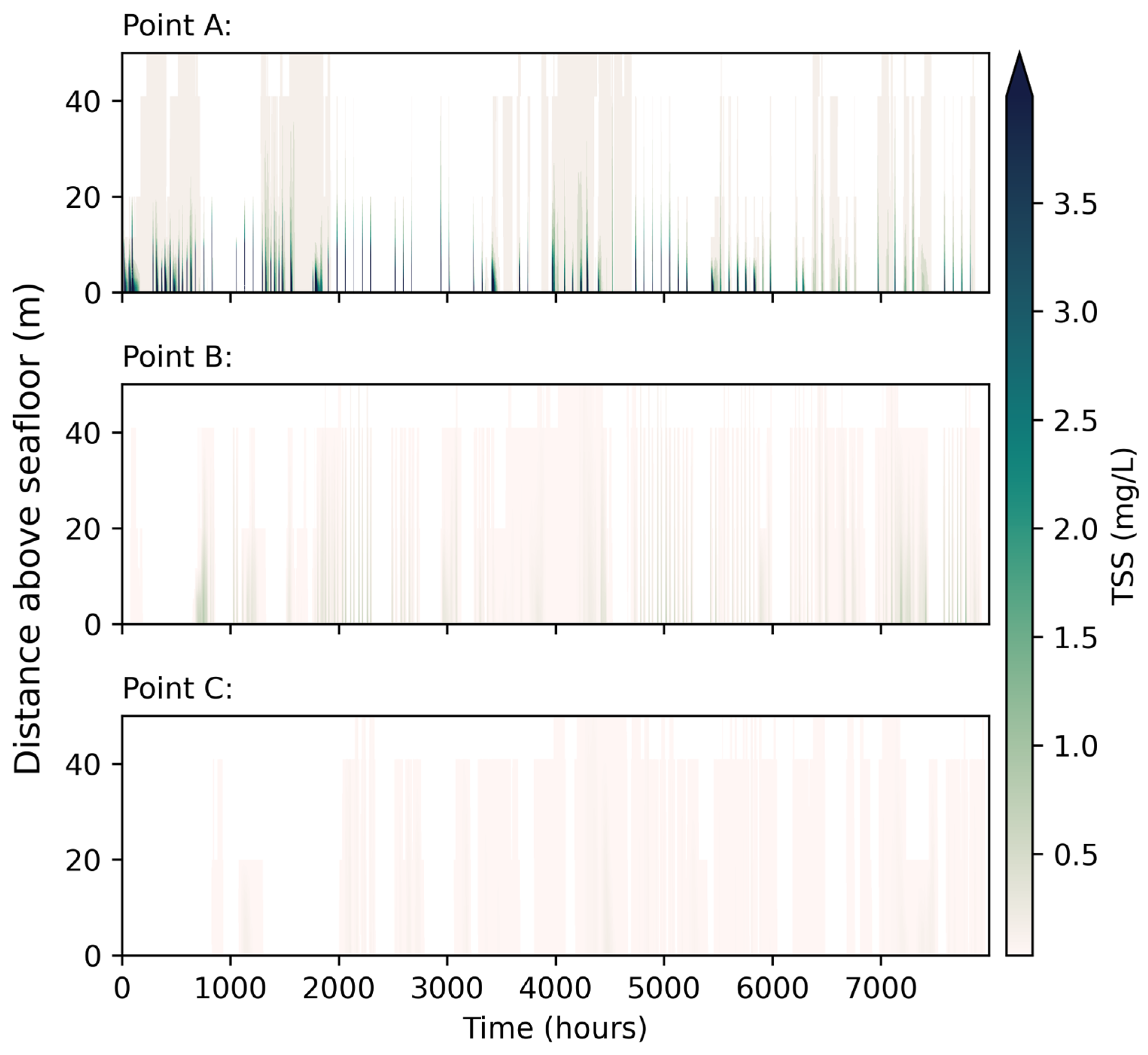
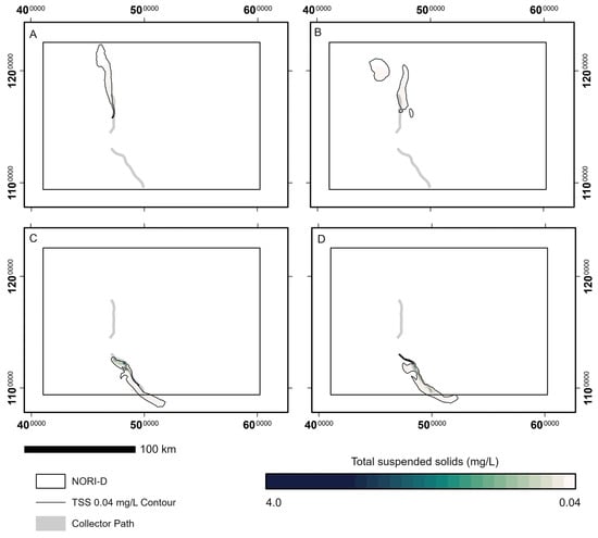
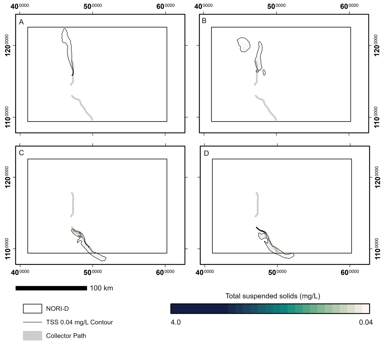
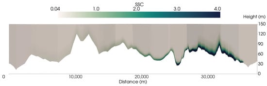
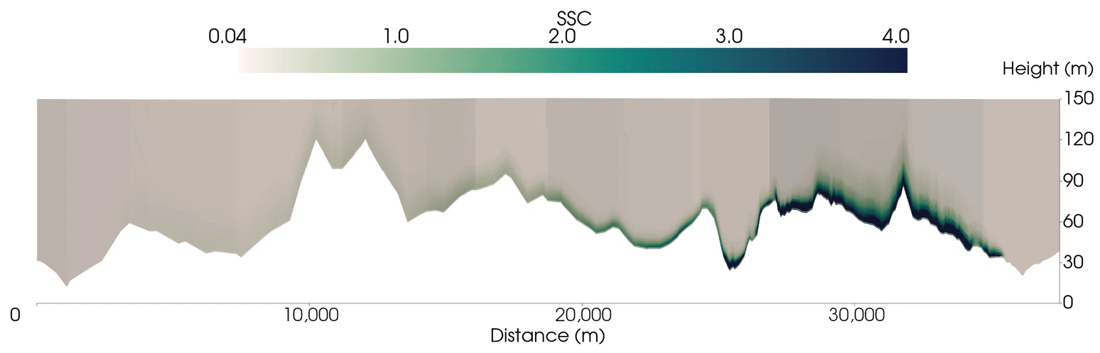
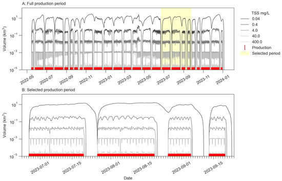
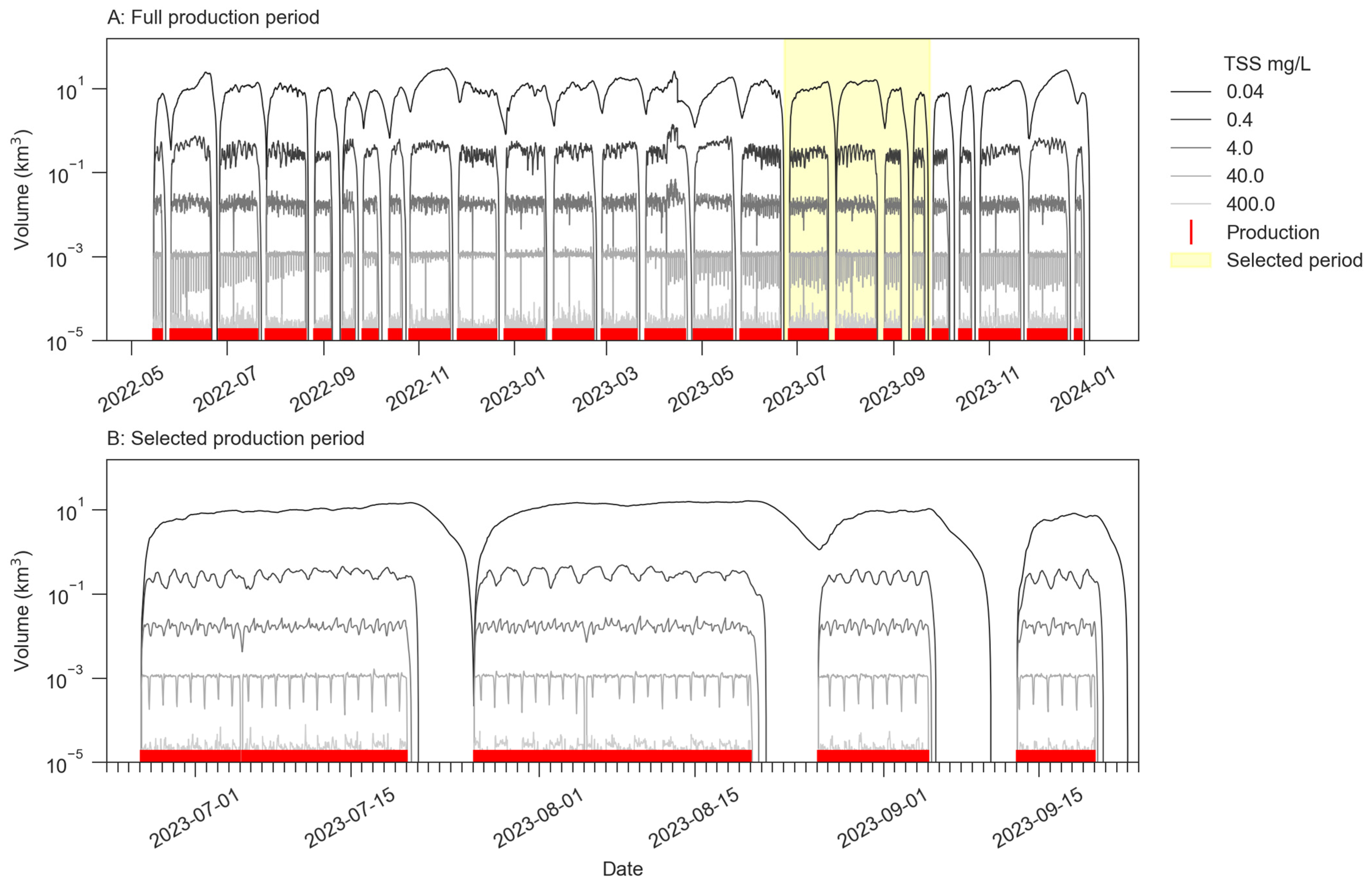
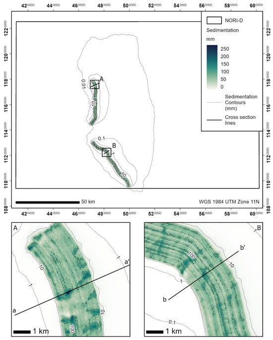
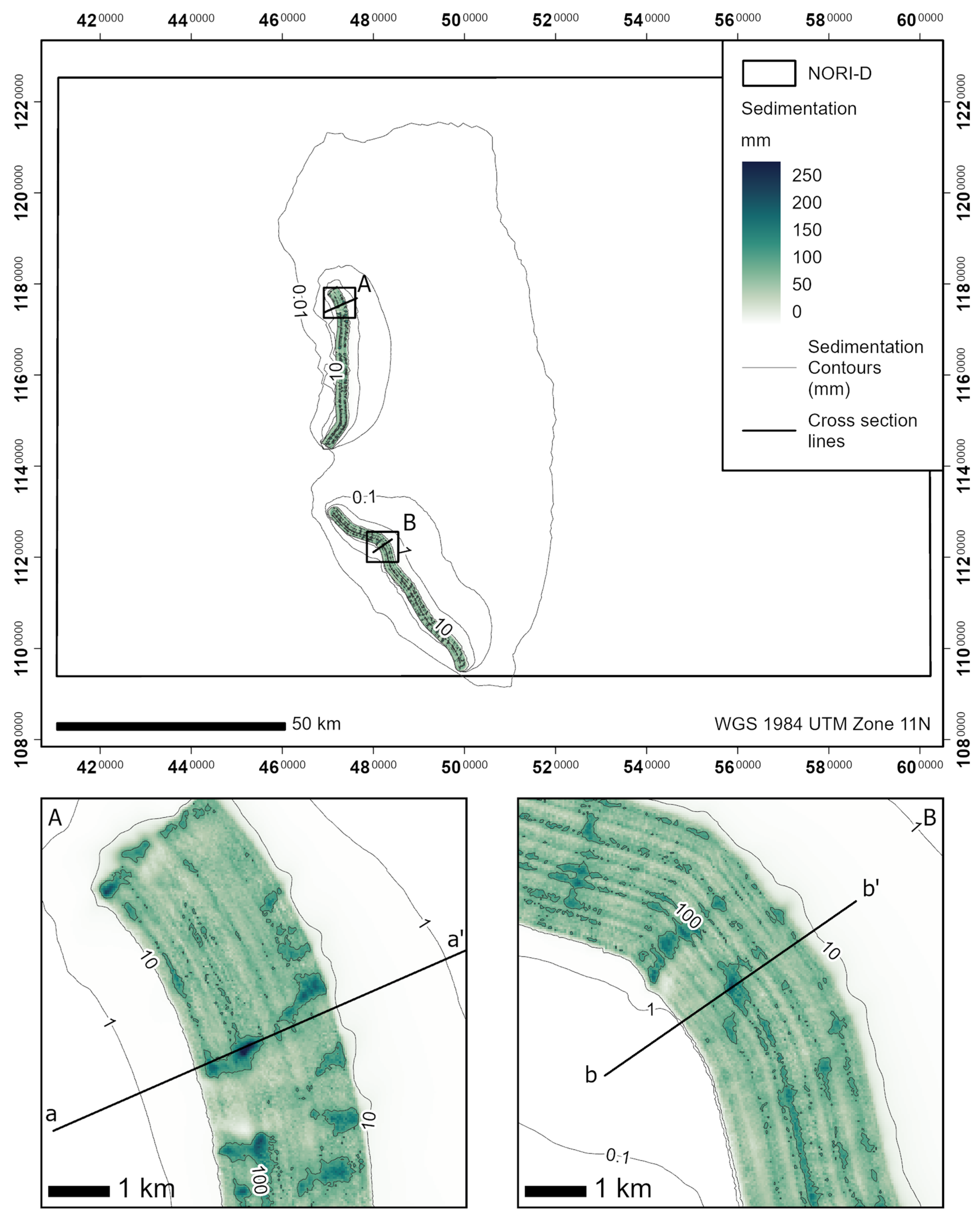
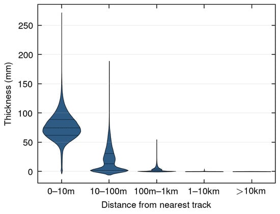
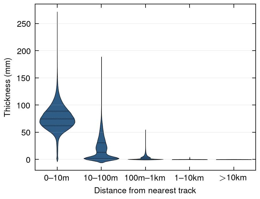
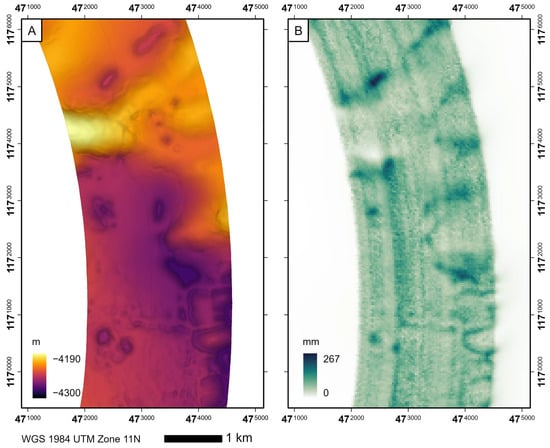
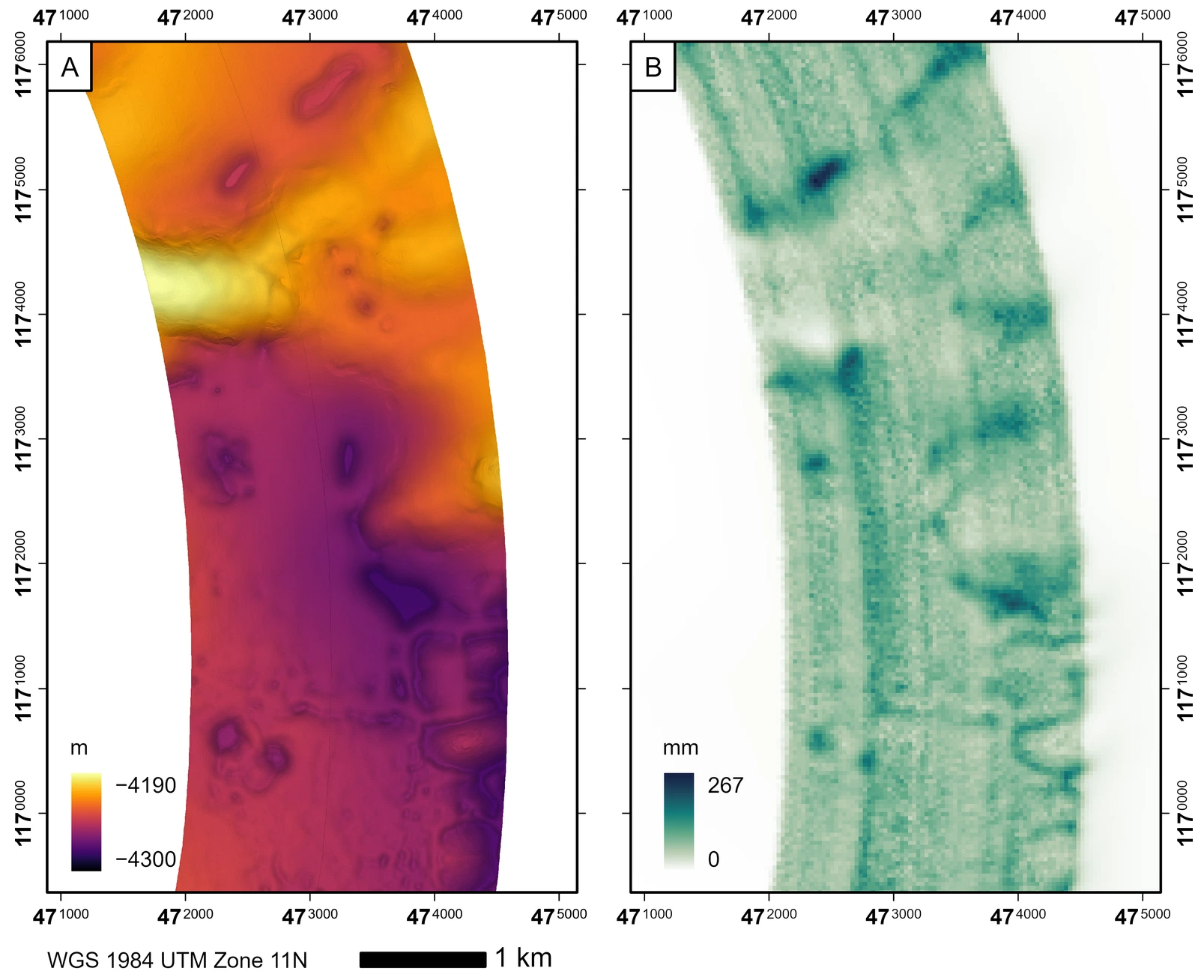
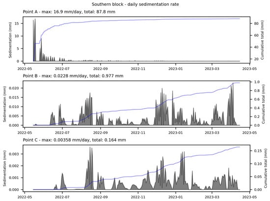
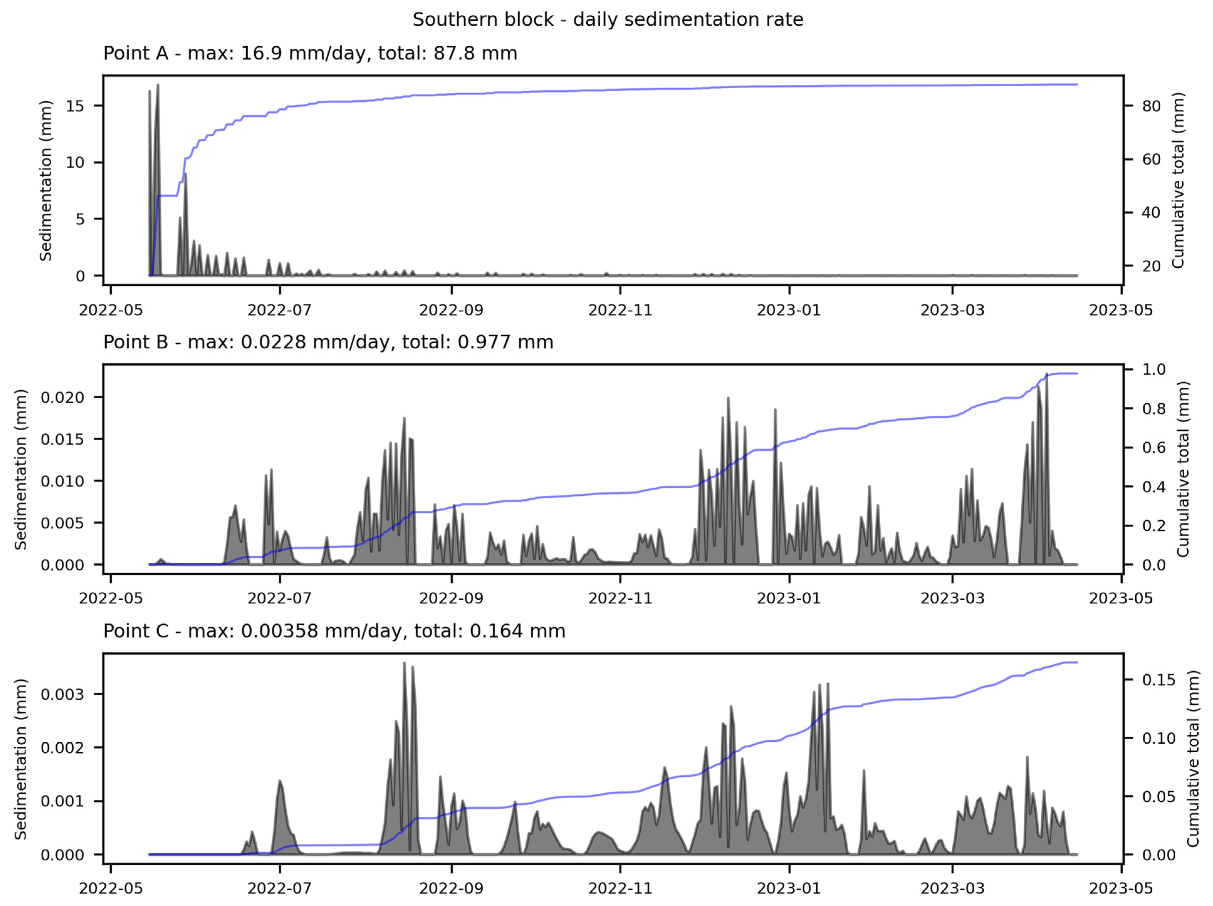

Disclaimer/Publisher’s Note: The statements, opinions and data contained in all publications are solely those of the individual author(s) and contributor(s) and not of MDPI and/or the editor(s). MDPI and/or the editor(s) disclaim responsibility for any injury to people or property resulting from any ideas, methods, instructions or products referred to in the content. |
© 2026 by the authors. Licensee MDPI, Basel, Switzerland. This article is an open access article distributed under the terms and conditions of the Creative Commons Attribution (CC BY) license.