Modeling Marine Traffic Density and Flow as S-100 Grid Hydrographic Data

Abstract

Marine traffic information supports the safe and efficient operation of ships and has been produced in various ways from Automatic Identification System (AIS) data. However, existing outputs differ in grid size, aggregation method, and format and cannot be used with charts on navigation equipment. This study defines historical marine traffic information, namely traffic density and flow, as gridded hydrographic data based on the International Hydrographic Organization (IHO) S-100 Universal Hydrographic Data Model. Based on a previously proposed high-resolution traffic flow model, an application schema, a Feature Catalogue, and a Portrayal Catalogue were designed, and the data were encoded in HDF5. Density is portrayed by color levels, and flow by arrow symbols that combine speed, density, and direction. A dataset was built from two years of AIS data for the coastal waters of Mokpo, Republic of Korea, and its values and portrayal rules were verified quantitatively. The density was displayed in a third-party S-100 viewer using only the catalogues and dataset, whereas the flow was displayed only in a simulator based on an in-house S-100 chart engine. These results show that historical marine traffic information can be defined, encoded, and portrayed as S-100 gridded data; operational interoperability remains to be verified.

1. Introduction

Marine traffic information is one of the basic types of information that support the safe and efficient operation of ships. In particular, information on how often ships pass through a given sea area, and in which direction and at what speed they mainly move, reveals traffic characteristics of the area that cannot be obtained from ship positions at a single moment. Such information is used in various fields, including ship route planning, traffic risk assessment, and vessel traffic services [1,2], and methods that generate routes by learning from historical passage data are also being studied for autonomous ships [3]. As Automatic Identification System (AIS) data, which record the position and speed of ships, have accumulated over long periods, research institutes and public agencies have produced marine traffic information in various ways [4,5,6,7]. However, the grid size, aggregation method, and output format differ among institutions and studies. Moreover, this information is mostly used in the form of reports or maps and is not provided as data that can be loaded and used together with charts on shipboard navigation equipment.

Meanwhile, the International Hydrographic Organization (IHO) developed S-100, the Universal Hydrographic Data Model, so that navigation equipment can handle diverse marine information in a common way and hydrographic information can be extended [8,9]. S-100 requires the data model, encoding, and portrayal to be defined for each Product Specification, and it specifies how to encode not only vector data but also grid coverages in the HDF5 format [8]. Gridded hydrographic products such as bathymetric surface (S-102), water level (S-104), and surface currents (S-111) follow this approach. With the Phase 1 Product Specifications coming into effect in 2026, these products have entered the stage of being used together with electronic navigational charts (ENCs) on S-100 Electronic Chart Display and Information Systems (ECDIS) [10,11,12,13]. The International Maritime Organization (IMO) has also revised the performance standards so that ECDIS newly installed from 2029 must support S-100 [14]. Marine information used in navigation systems is therefore expected to be provided increasingly as S-100 products.

However, marine traffic information is not yet sufficiently addressed within the S-100 framework. Traffic-related Product Specifications have been developed in the S-100 family, but they mainly deal with management and regulatory information, such as vessel traffic service areas and routing measures, or with the current position and route plan of individual ships [15,16,17,18]. It is difficult to find a case in which traffic information showing how ships usually move in a sea area has been defined as a Product Specification. Nor can the outputs of existing marine traffic studies fill this gap directly. S-100 data must be accompanied by a Feature Catalogue, which defines the meaning, units, and value ranges of attributes, and a Portrayal Catalogue, which defines how they are displayed, both in machine-readable form [8]. Such specifications are not available for the research outputs [5,19].

This study therefore aims to define historical marine traffic information, namely traffic density and flow aggregated from AIS data accumulated over a given period, as S-100-based hydrographic information so that it can be delivered to and displayed on navigation systems in the same way as other hydrographic information. The information is produced with the high-resolution traffic flow model proposed in a previous study [19], and this study focuses on transferring its results into the S-100 framework. Three research questions are addressed: (i) whether historical marine traffic information can be defined with an S-100 application schema and Feature Catalogue; (ii) whether it can be encoded in HDF5 according to S-100 Part 10c without loss of values; and (iii) whether it is portrayed according to the rules of its Portrayal Catalogue in S-100 display environments, namely a third-party viewer and a simulator based on an in-house S-100 chart engine. Following the IHO guidelines for creating S-100 Product Specifications [20], the modeling proceeded in the order of requirements derivation, design of the application schema and Feature Catalogue, and design of the Portrayal Catalogue. Because traffic flow must express speed, density, and direction in a single symbol, portrayal rules for this purpose were also designed. The data were encoded in the HDF5 format, which is suited to gridded hydrographic information. The model was applied to traffic information for the coastal waters of Mokpo, Republic of Korea, to answer these questions through quantitative validation of the dataset, the catalogues, and the portrayal rules. The traffic model itself is adopted from [19]; the contributions of this study are the application schema and Feature Catalogue for historical marine traffic information, the Portrayal Catalogue with portrayal rules that combine several attributes for each grid cell, the HDF5 encoding with dataset metadata, and their validation.

The remainder of this paper is organized as follows. Section 2 reviews the structure of S-100 and the traffic-related Product Specifications, summarizes the modeling, encoding, and portrayal of gridded data, and then reviews studies on marine traffic information and on S-100 data models. Section 3 derives the requirements for marine traffic information and designs, in turn, the application schema, the Feature Catalogue, the Portrayal Catalogue for density and flow, and the HDF5 encoding structure. Section 4 builds a dataset from traffic information for the coastal waters of Mokpo and presents the validation and visualization results, with density displayed in a third-party S-100 viewer and flow in a simulator based on an in-house S-100 chart engine. Section 5 discusses the features and limitations of the proposed model and presents the conclusions.

2. Background and Related Work

This section summarizes the S-100 framework and the related work that form the background of this study and identifies the research gaps addressed in this study.

2.1. S-100 Framework and Traffic-Related Product Specifications

S-100 is the universal hydrographic data standard developed by the IHO, and it provides a framework for defining, exchanging, and portraying diverse marine information in a consistent structure. An S-100 product generally requires four core elements: an application schema, a Feature Catalogue, a Portrayal Catalogue, and an encoding. The application schema is a structured data model that defines the features, attributes, spatial information, and relationships between objects used in a specific marine information product, and it specifies how the information is organized and linked. The Feature Catalogue is a data dictionary that standardizes the names, definitions, data types, and permitted values of the features and attributes in the application schema, so that data can be created and interpreted with the same meaning. The Portrayal Catalogue defines how features and attribute information are visually presented on screen and supports consistent visualization through symbols, colors, line and area styles, and conditional portrayal rules. The encoding specifies the format in which the defined information is stored and exchanged as data files, and formats such as GML, XML, and HDF5 are used depending on the characteristics of the data.

The marine traffic density and flow addressed in this study are traffic information produced by accumulating AIS data over a given period, so it is first necessary to examine what information the existing S-100-based traffic-related Product Specifications cover. Among them, S-127 and S-212 are intended for the provision of marine traffic management information and for information exchange between vessel traffic services (VTS) and ships, respectively, and their domains are the closest to that of the proposed model. S-127 (Marine Traffic Management) is a Product Specification that provides, in standardized form, marine traffic management information related to ship operation, such as VTS, pilotage, routing measures, and ship reporting systems. It provides structured information on the traffic management services, operational regulations, and managed areas that apply in a given sea area, and the location of each service is indicated by simplified vector geometry (points, curves, and surfaces) together with its service area, the services offered, and contact instructions. S-127 supplements the ENC and serves to link more regulatory information to locations than the ENC does [15]. The data are encoded in GML and updated as needed, and portrayal is not defined. S-212 (VTS Digital Information) is a Product Specification for the digital exchange of the traffic information and navigational assistance information that VTS provide to ships and related organizations, and it supports the digitalization of VTS services between ship and shore. S-212, which is under development by the International Organization for Marine Aids to Navigation (IALA), covers messages exchanged between VTS and ships in real time or near real time, and one dataset contains one message [16]. The message currently defined is the traffic clearance message, which includes anchorage assignment; the data are encoded in GML, and there are no plans to develop a Portrayal Catalogue. In addition, S-210 (Inter-VTS Exchange Format) is a Product Specification for exchanging ship positions, tracks, and traffic situation information between different VTS centers in a standardized format, and it aims to improve the continuity of ship information between adjacent VTS areas and the interoperability between VTS systems [17]. As shown in Table 1, both S-127 and S-212 deal with marine traffic, but they provide management information on areas and services or ship-specific messages in vector form and do not include historical traffic information for a sea area. By defining as S-100 data the historical marine traffic information that these existing standards do not cover, this study seeks to complement the existing S-100 marine traffic information framework.

Table 1. Comparison of traffic-related S-100 Product Specifications and the proposed model in terms of target information, nature of information, spatial representation, encoding, and Portrayal Catalogue.

Item	S-127 Marine Traffic Management [15]	S-212 VTS Digital Information [16]	Proposed Model
Target information	VTS, pilotage, routing measures, ship reporting	Traffic clearance, anchorage assignment	Traffic density and flow by sea area
Nature of information	Management and regulatory information (updated as needed; frequency set by the producer)	Ship-specific clearance messages (real time; one message per dataset)	Statistical information accumulated over a given period
Spatial representation	Vector	Vector	Grid
Encoding	GML	GML	HDF5
Portrayal Catalogue	Not defined	No plans for development	Defined (Lua, SVG)

2.2. Grid Coverage Modeling, HDF5 Encoding, and Portrayal

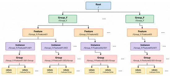
To standardize information that varies continuously in space, such as depth, currents, the marine environment, and risk, S-100 systematically defines grid coverage modeling, HDF5-based encoding, and portrayal rules. S-100 Part 8 defines the structure for modeling spatial information in the form of grids and coverages; it organizes the sea space into cells and allows values such as depth, current, environmental information, and risk to be represented in each cell. S-100 Part 10c defines the encoding rules for storing and exchanging such gridded data in the HDF5 format. Using the group, dataset, and attribute structure of HDF5, large volumes of gridded information and time-series data can be managed efficiently. S-100 Part 9A allows visual presentation such as colors, symbols, lines, and areas to be applied according to the attribute values of the data through Lua-based portrayal rules; in particular, different portrayal rules can be applied according to the values or levels of gridded data so that their spatial distribution is shown intuitively. S-100-based gridded information can therefore be organized as a system consisting of the definition of the grid structure through Part 8, storage and exchange in HDF5 through Part 10c, and visual presentation through Part 9A. Figure 1 shows the general hierarchical structure of an S-100 HDF5 file.

Figure 1. General hierarchical structure of an S-100 HDF5 file (Root → Group_F → Feature → Instance → Group → values).

Gridded S-100 products store one or more values in each cell, and the Portrayal Catalogue converts them into colors or symbols for display [8]. As shown in Table 2, bathymetric surface (S-102) is colored according to depth ranges [10]; water level (S-104) has no Portrayal Catalogue of its own and is used to adjust the depth and uncertainty values of the ENC and S-102 [11]; and surface currents (S-111) are drawn as arrows using current speed and direction [12]. The color and size of the S-111 arrow are determined by current speed alone, and when a wide area is viewed, the arrows are thinned at regular intervals [12]. The density of the proposed model is portrayed by color fill, as in S-102, whereas the flow differs from S-111 in that both speed and density are taken into account when the arrow is selected.

Table 2. Comparison of gridded products: attributes, units, and portrayal of S-102, S-104, S-111, and the proposed model.

Item	Target Information	Grid Values (Attribute, Unit)	Portrayal
S-102 [10]	Bathymetry	depth (m) uncertainty (m, optional)	Color fill by depth range (depth zone colors adapted from S-52)
S-104 [11]	Water level	waterLevelHeight (m) waterLevelTrend (decreasing, increasing, steady) uncertainty (m, optional)	No Portrayal Catalogue of its own Used for water level adjustment of ENC and S-102 depths
S-111 [12]	Surface currents	surfaceCurrentSpeed (knots) surfaceCurrentDirection (clockwise from true north, °)	Arrows colored by nine speed bands and sized by speed, rotated to the direction of flow Arrows thinned when zoomed out
Proposed model (density)	Marine traffic density	trafficDensity (level 1–15) trafficDensityDimension (level 1–15)	Color fill in 15 levels
Proposed model (flow)	Marine traffic flow	trafficSpeed (knots) trafficDirection (°) trafficDensityDimension (level 1–15)	5 speed levels × 15 density levels = 75 arrow symbols, rotated to the direction of travel

2.3. Related Work

As AIS data have accumulated, marine traffic information has been produced for various purposes. Kim et al. [4] calculated the average ship length, average speed, and passage frequency for each cell in the grid system of the Korea Hydrographic and Oceanographic Agency and combined them into a ship traffic index, and Lee et al. [1] used routes extracted from spatial–temporal density for route search. A harbor hazard map based on a traffic hazard index [2] and deep-learning-based traffic flow prediction [21] have also been proposed. As public services, EMODnet and HELCOM provide vessel density maps on a 1 km grid [6,7]. Some studies have sought to represent the direction and speed of movement in addition to density. Lee et al. [5] overlaid a density heat map on a grid of about 100 m and representative direction arrows on an S-57-based ENC for the approach channel to Mokpo, and Oh et al. [19] proposed a traffic flow model that represents density, dominant direction, and average speed in a single arrow symbol on a 3″ grid. However, these studies and services differ in grid system, aggregation unit, and classification criteria, and they provide their results as maps, images, or agency-specific GIS grids rather than as S-100-based electronic chart data. Even where the results were shown together with an ENC, the analysis results were overlaid as images, and no case was found in which the meaning of the attributes and the display method were defined in machine-readable form together with the data. Consequently, for navigation equipment to read and display such information in the same way as other hydrographic information, separate conversion and display functions are required for each type of information.

Meanwhile, the traffic information provided in the maritime field mainly concerns the current traffic situation or traffic management. IALA defines the VTS traffic image as the current picture of the vessels and their movements in a VTS area [22], and Kim et al. [23] developed a system that fuses AIS data in real time and displays ship trajectories for a remote operation center for autonomous ships. Guo et al. [24] designed an e-Navigation service that provides traffic organization information to autonomous ships, and S-127 and S-212, described in Section 2.1, deal with traffic management areas and rules and with ship-specific traffic clearance and anchorage assignment [15,16]. Thus, existing studies and S-100 products provide only the current state of individual ships or management and instruction information, and historical traffic information showing how ships usually move in a sea area is not provided as S-100 data. Lee et al. [5] also pointed out that the current S-101 has no means of showing traffic behavior information such as traffic density and flow, and identified defining it within the S-100 framework as future work.

Studies that define new types of information as S-100 products have also continued. Lee et al. [25] defined historical marine casualties with an application schema, a Feature Catalogue, and a Portrayal Catalogue, and for gridded data, Luo et al. [26] proposed a model, based on S-102, that stores high-density bathymetric data in an HDF5 hierarchical structure. Regarding portrayal, Tomczuk [27] tested Lua-based portrayal rules with S-101 ENCs, Lee et al. [28] compared the symbols and feature portrayal of several Product Specifications from the viewpoint of ECDIS and VTS software implementation, and Cho et al. [29] analyzed the security issues that arise when portrayal scripts are executed on S-100 ECDIS. However, the studies on gridded models addressed natural phenomena such as depth, and the portrayal studies mainly dealt with ENCs and vector products. Surface currents (S-111), which are displayed as arrows on a grid, also determine the color and size of the arrow from current speed alone [12]. The traffic flow in this study must express speed, density, and direction in a single symbol and therefore requires grid portrayal rules that combine several attributes, but no case addressing such rules was found within the scope reviewed. Table 3 summarizes the results of this review as three research gaps.

Table 3. Research gaps identified from the review of previous studies.

Gap	Description	Supporting References
G1 Type of information	Traffic information for navigation support and the traffic-related S-100 products deal with the current state of individual ships (VTS traffic image, real-time traffic display) or with management and instruction information (traffic management areas and rules, traffic clearance and anchorage assignment). Historical traffic patterns of a sea area (density and flow) are not provided as S-100 data.	[5,15,16,22,23,24]
G2 Lack of standardization of marine traffic information	Information on marine traffic density, flow, routes, and risk is produced by studies and services, but the grid systems, aggregation units, and classification criteria differ, and the results are provided as maps, images, or agency-specific GIS grids. Because the attributes and display methods are not defined in machine-readable specifications, the information cannot be read and displayed in the same way as other hydrographic information.	[1,2,4,5,6,7,19,21]
G3 Portrayal	Studies on gridded S-100 models address natural phenomena (depth), and portrayal studies mainly address ENCs and vector products. Portrayal rules that select a symbol from several attributes (speed and density) for each grid cell and rotate it by direction were not found within the scope reviewed. The S-111 arrow depends on a single attribute, current speed.	[12,26,27,28,29]

3. Modeling of Marine Traffic Information

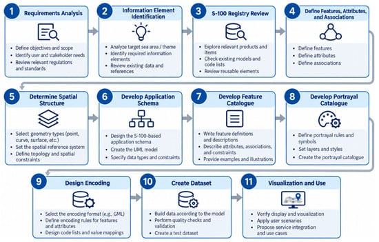
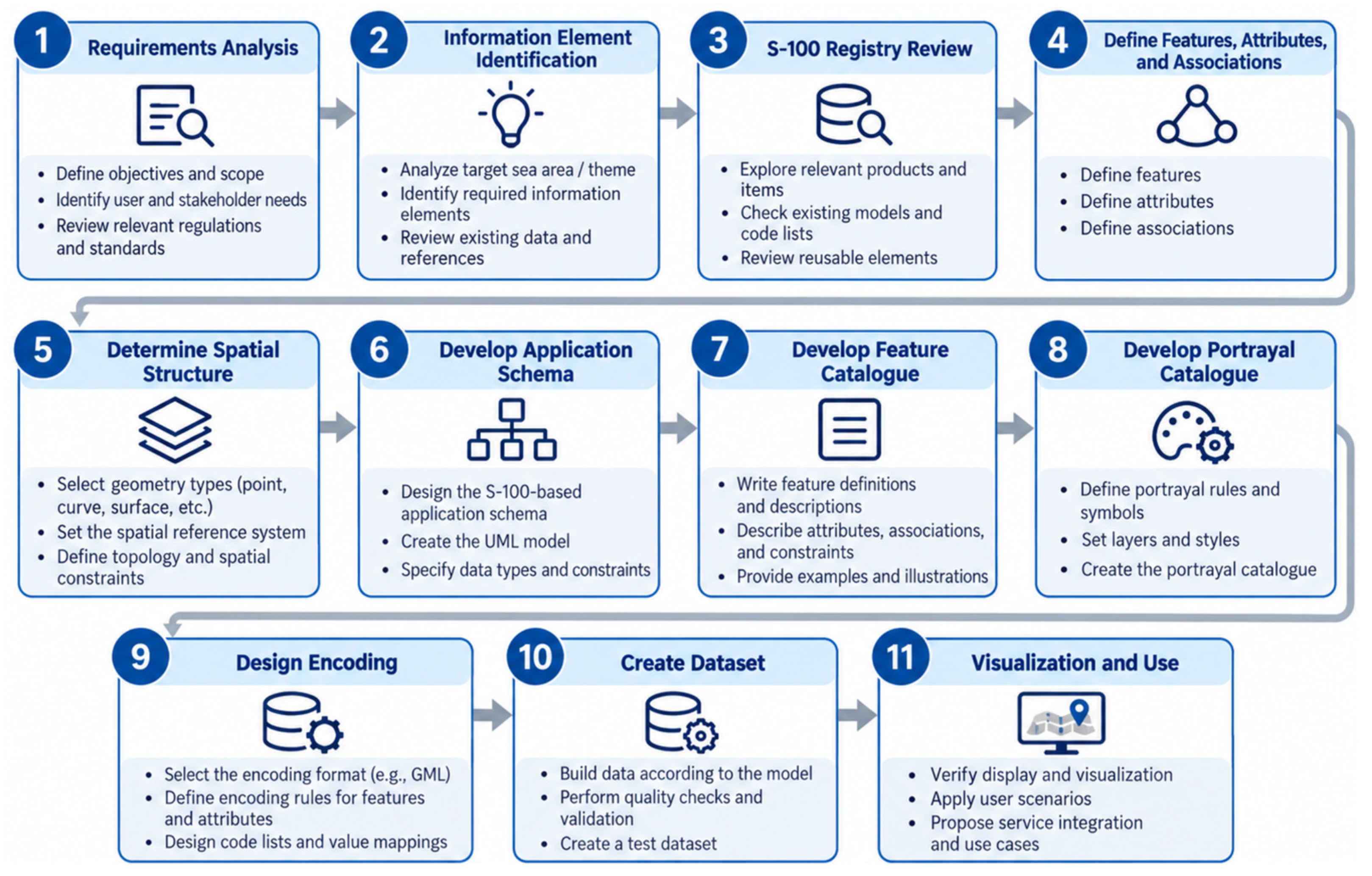
S-100-based modeling is the process of defining marine information in a standardized data structure and implementing it as an actual dataset. Following the procedure in Figure 2, the requirements were derived first (Section 3.1); the application schema and the Feature Catalogue were then designed (Section 3.2 and Section 3.3), followed by the Portrayal Catalogue (Section 3.4) and the HDF5 encoding (Section 3.5).

Figure 2. Procedure for S-100-based modeling.

3.1. Requirements for the Traffic Model

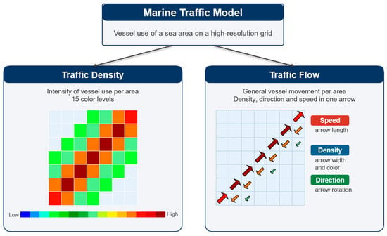
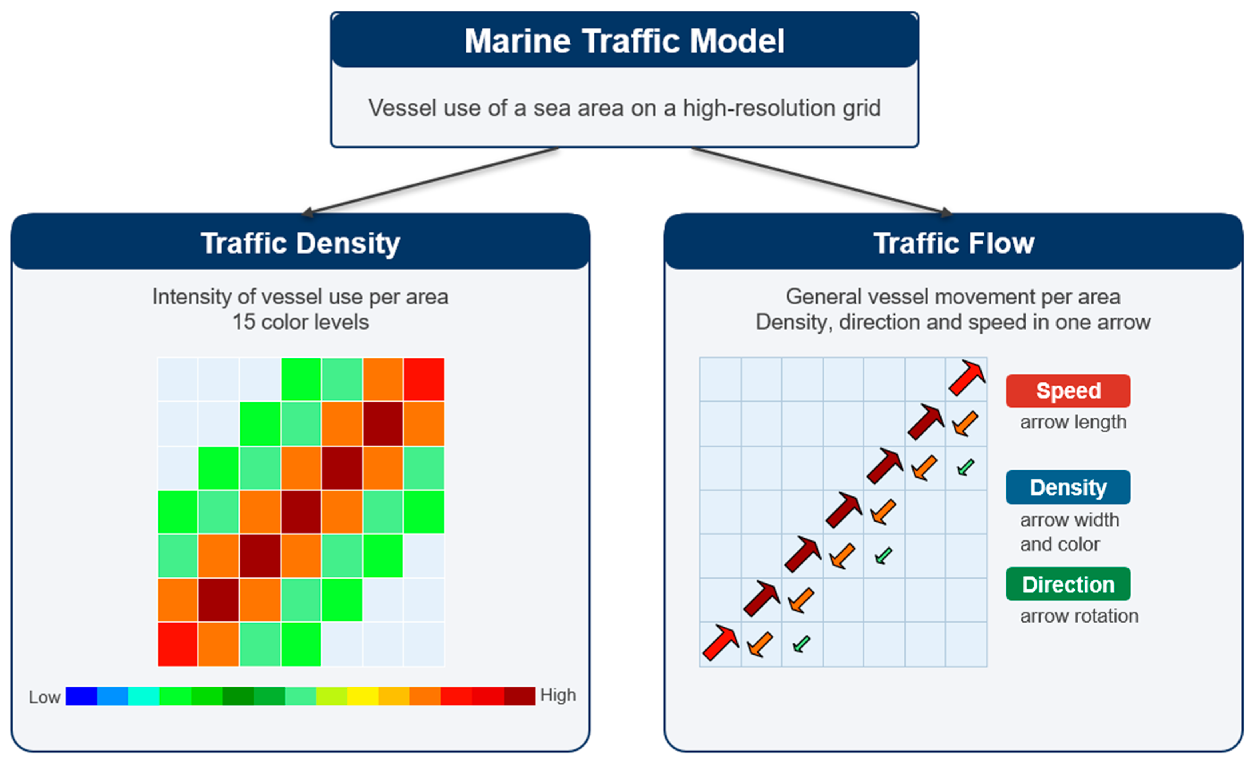
The information defined as S-100 data in this study is the output of the high-resolution marine traffic model proposed in a previous study [19]. The model uses AIS data provided by the Ministry of Oceans and Fisheries of the Republic of Korea for the coastal waters of Mokpo from 1 January 2022 to 31 December 2023 (UTC). The data were preprocessed as described in Section 2.2 of [19]: missing and erroneous values and points on land were removed, and tracks were split where the distance between two consecutive reports exceeded 1 nautical mile. Records at or below 2 kn were then excluded, because such vessels are unlikely to be under way and some vessels do not change their navigational status when at anchor [19]. The area is divided into a regular grid with a spacing of 0.00083333° (3″) in latitude and longitude, which is about 92.6 m north–south and 76.2 m east–west in the study area. This grid size was chosen in [19] because it corresponds to the length of medium-sized vessels, is sufficiently larger than the positional accuracy of AIS (about 10 m), and represents narrow channels and port approaches in more detail than the 500 m–1 km grids of previous studies. As shown in Figure 3, the model consists of two types of information. Because the details of the calculation method are given in [19], the definitions needed for S-100 modeling are summarized below.

Figure 3. Composition of the marine traffic model.

Traffic density is an indicator of the frequency of traffic passing through a cell and, as in Section 2.4 of [19], is computed as the number of AIS samples (position reports) recorded in the cell during the reference time period. Because the AIS sample count also depends on the time a vessel spends in the cell and on the reporting interval, it is not equivalent to the number of vessel passages; the measured quantity is therefore referred to in this paper as the passage frequency computed from the AIS sample count. The sample counts are classified into 15 levels on a logarithmic scale (Section 3.4). Traffic flow is described by the dominant direction and the mean speed in that direction. As in [19], the course over ground (COG) of each AIS sample is assigned to one of 36 sectors of 10°:

$$s = ⌊{\displaystyle \frac{COG}{10°}}⌋ \left(mod 36\right)$$

(1)

where COG is the course over ground of the sample in degrees (0–360) and s is the index of the directional sector (0–35). The sector with the largest number of samples is taken as the dominant direction of grid cell (i, j):

$$s_{ij} = {argmax}_s \left\{n_{ij}\left(s\right)\right\}$$

(2)

where n_ij(s) is the number of AIS samples in grid cell (i, j) that fall into sector s. When two or more sectors have the same largest number, the sector with the smallest index, that is, the first sector clockwise from true north, is selected. A dominant direction is used instead of an average direction, because averaging opposing courses such as 90° and 270° yields a direction that represents neither. The mean speed is the average speed over ground of the AIS samples in the dominant sector:

$$v_{ij} = {\displaystyle \frac{\sum SPD}{n_{ij}\left(s_{ij}\right)}}$$

(3)

where SPD is the speed over ground (kn) of each AIS sample in the dominant sector s_ij. The density level attached to the flow is calculated from the samples in all directions and therefore represents all traffic in the cell. Table 4 compares the components adopted from [19] with those developed in this study, and the rest of this section summarizes the requirements for transferring the model output into S-100 data.

Table 4. Components adopted from the previous study [19] and components developed in this study.

Component	Previous Study [19]	This Study
AIS data and preprocessing	Mokpo coastal waters, 2022–2023; preprocessing in Section 2.2 of [19]; records at or below 2 kn excluded	Adopted
Grid	Regular 3″ grid	Adopted; encoded as an S-100 grid coverage
Traffic density	AIS sample count per cell; 15 logarithmic levels	Adopted; stored as integer attributes with class boundaries in the metadata
Traffic flow	Dominant direction (36 sectors of 10°) and mean speed	Adopted; stored as trafficDirection (sector center) and trafficSpeed
Visualization	Maps with colored grid cells and arrows (length: 5 speed classes; width: 5 density categories; color)	75 SVG symbols and Lua portrayal rules in an S-100 Portrayal Catalogue
Data model	–	Application schema and Feature Catalogue (S100FC)
Encoding	–	HDF5 according to S-100 Part 10c, with metadata
Validation	Visual analysis of traffic patterns	Schema and structure checks, value preservation, portrayal-rule tests, display in a third-party viewer and a simulator

First, because the information is produced on a regular grid of cells, it must be represented as a grid coverage rather than as individual points or curves as in S-57 and some S-100 products. Second, because density and flow differ in how they are displayed and in their intended use, it must be possible to display and select each of them independently, and the flow must include the density level used to determine the width and color of the symbol. Third, the meaning, unit, and range of each value must be clear. Density is expressed as a level from 1 to 15, speed in knots, and direction as intervals obtained by dividing the angle measured clockwise from true north (°) into steps of 10°. Fourth, because about 64% of the cells in the study area contain no retained AIS observations, cells without values must be distinguishable from valid values. In particular, 0 cannot be used as the fill value for direction because 0° is a valid value. Fifth, because the information is the result of accumulation over a given period, the reference time period must be recorded with the data. Finally, density must be displayed in 15 color levels, and flow as arrows that reflect speed, density, and direction. Table 5 summarizes these requirements and the design elements that address them.

Table 5. Requirements for S-100 modeling of marine traffic information.

Requirement	Characteristics of the Source Model	Design Response (Section)
Spatial representation	Regular grid of 0.00083333° (3″), 540 × 420 cells	Grid coverage features, HDF5 regular grid (3.2, 3.5)
Separation of information	Two types of information: density and flow	Two features: MarineTrafficDensity, MarineTrafficFlow (3.2)
Attributes and value ranges	Density level 1–15, speed (kn), direction (°)	Attribute definitions, units, and value ranges (3.3)
Missing data	144,965 cells without retained AIS observations; 0° is a valid direction	Fill value of 1,000,000 (3.3, 3.5)
Reference time period	Accumulated over 2022–2023	referenceTimePeriod attribute (3.3)
Display	Color for density, arrows for flow	15-level color rule, 75 flow symbols (3.4)

3.2. Application Schema

The application schema is a conceptual model that defines the features and attributes handled by the product, and their relationships, as a UML class diagram, and it serves as the basis for the Feature Catalogue and the dataset encoding [8]. In this study, the application schema was prepared with the UML modeling tool Enterprise Architect (version 17) in the following order. First, the information that must be displayed independently according to the requirements in Section 3.1 was identified as features, and each feature was created as a class in accordance with the S-100 General Feature Model [8,30]. Next, the attributes of each feature and their data types and multiplicities were determined, and attributes whose values are selected from a fixed list were defined separately as enumerations. Finally, the spatial representation of each feature was specified as a spatial attribute. Classes and attributes are distinguished by stereotypes: geographic features are marked “FeatureType(Geo)”, simple attributes “SimpleAttribute”, spatial attributes “SpatialAttribute", and enumerations "enumeration”.

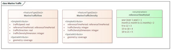
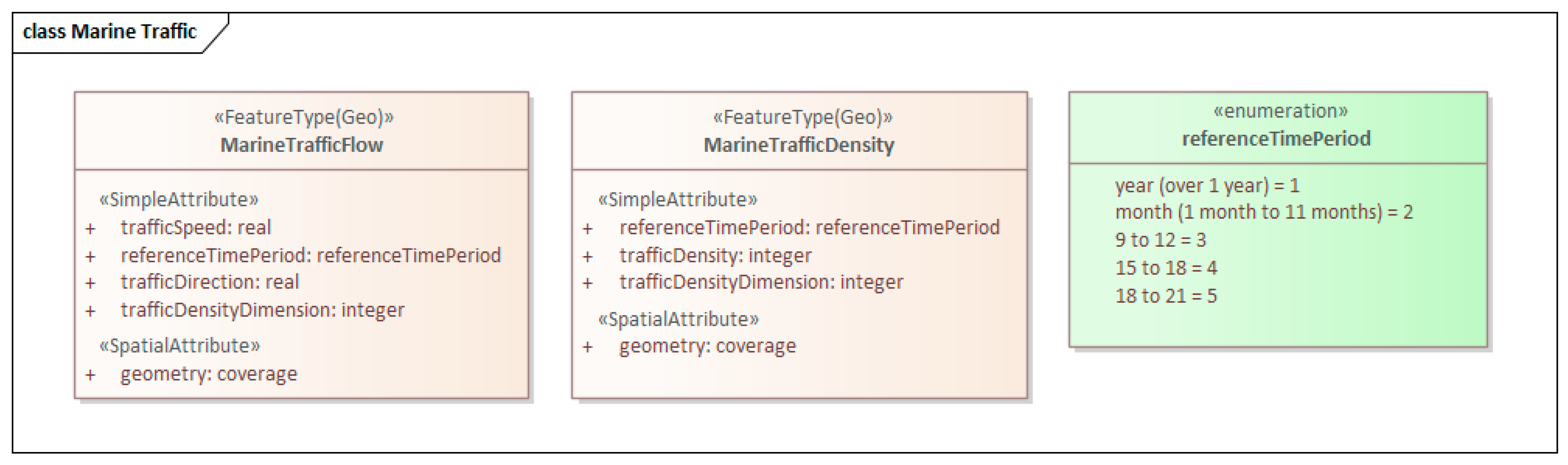
As shown in Figure 4, the schema consists of two geographic features: MarineTrafficDensity, which represents traffic density, and MarineTrafficFlow, which represents traffic flow. Both features have a grid coverage as their spatial attribute and are therefore encoded as gridded data with attribute values in each cell. MarineTrafficDensity has the level of passage frequency computed from the AIS sample count (trafficDensity) and the density level considering the size of vessels (trafficDensityDimension); MarineTrafficFlow has the average speed of the ships moving in the dominant direction (trafficSpeed), the dominant direction (trafficDirection), and the density level (trafficDensityDimension). Both features share the reference time period (referenceTimePeriod), which is defined as an enumeration that distinguishes yearly, monthly, and time-of-day accumulation. Following the S-100 naming conventions, feature names are written in UpperCamelCase and attribute names in lowerCamelCase. Table 6 lists the attributes, data types, and multiplicities of each feature.

Figure 4. UML class diagram of the application schema.

Table 6. Features and attributes of the application schema.

Feature	Attribute	Data Type	Multiplicity	Description
MarineTrafficDensity	trafficDensity	integer	1	Level of passage frequency computed from the AIS sample count (1–15)
	trafficDensityDimension	integer	1	Density level considering vessel size (1–15)
	referenceTimePeriod	enumeration	0.1	Reference time period
	geometry	coverage	1	Grid coverage
MarineTrafficFlow	trafficSpeed	real	1	Average speed of ships in the dominant direction
	trafficDirection	real	1	Dominant direction of travel
	trafficDensityDimension	integer	1	Density level considering vessel size (1–15); determines symbol width and color
	referenceTimePeriod	enumeration	0.1	Reference time period
	geometry	coverage	1	Grid coverage

The two features were defined independently of each other rather than grouped under an abstract parent feature. The only attributes they share are the reference time period and the density level, and because their display methods and uses differ, with density portrayed as color fill and flow as symbols, mariners must be able to display or hide each of them separately. In addition, the flow feature carries the density level as its own attribute instead of referencing the density feature. Because the flow symbol is selected for each cell from the combination of speed and density level, this allows the portrayal rule to determine the symbol from the values of a single feature. Because the density levels are discrete categories from 1 to 15, trafficDensity and trafficDensityDimension are defined as integers; the fill value of 1,000,000 (Section 3.3) can also be represented as an integer. trafficDensityDimension is defined as the density considering the size of vessels. Because vessel size was not reflected in the dataset of this study, the same level is stored in both attributes, and the two values were confirmed to agree in all cells with values (Section 4.2). No information types or associations between features were used.

3.3. Feature Catalogue

The Feature Catalogue is a document that describes the content of the application schema in XML so that it is machine-readable; navigation equipment loads it to interpret the meaning of the features and attributes contained in a dataset [8]. The Feature Catalogue in this study was prepared with the XML editor Altova XMLSpy (version 2026) in accordance with the Feature Catalogue schema (S100FC) of S-100 Edition 5.2. Following the product name, field of application, version, and producer information, it defines 5 simple attributes and 2 feature types. A name, definition, code, and data type are given for each attribute. For each feature type, the attributes it may have, their multiplicities, and their permitted values are specified through attribute bindings; the feature use type is set to geographic and the permitted geometric primitive to coverage, making explicit that both features are gridded data. The Feature Catalogue was validated against the S100FC schema (XSD) in XMLSpy and was confirmed to conform to the schema.

Table 7 lists the attributes defined in the Feature Catalogue. The reference time period (referenceTimePeriod) is defined as an enumeration with five values, from 1 (accumulation over one year or longer) to 5 (18:00–21:00), and the permitted values in the attribute bindings of both features are restricted to these five values. The value identifies the type of accumulation of a dataset (yearly, monthly, or time of day); a separate dataset is produced for each type, and the dataset in this study is a yearly accumulation (Section 4.1); the actual observation period is recorded separately in the HDF5 metadata (Section 3.5). The speed and direction attributes (trafficSpeed and trafficDirection) are of real type, and the two density attributes are integers; the units and value ranges of all attributes are recorded in the HDF5 file of the dataset together with the attribute codes. Speed is specified as 0–30 in knots, direction as 0° or more and less than 360° clockwise from true north, and the density level as 1–15. Following Clause 4.4.2.1 of S-102 Edition 3.0.0 [10], a fill value of 1,000,000, which lies outside the valid range of every attribute, is applied to all attributes in cells without retained AIS observations. These cells include land cells, water cells in which no AIS report was recorded, and water cells with only reports at or below 2 kn, so a lack of retained observations does not mean that no traffic occurred. Because 0° is a valid value for direction, 0 is not used as the fill value and a value outside the range is used instead. Since the attribute codes in the Feature Catalogue match the codes recorded in the dataset, navigation equipment can compare the two to interpret the meaning and unit of each value.

Table 7. Attributes defined in the Feature Catalogue.

Attribute	Definition	Data Type	Unit	Value Range
trafficDensity	Level of passage frequency, computed from the number of AIS samples recorded in the cell during the reference time period.	integer	–	1–15
trafficDensityDimension	Density considering the size of vessels; determines the width and color of the flow symbol.	integer	–	1–15
trafficSpeed	Average speed over ground of ships moving in the dominant direction.	real	knot	0–30
trafficDirection	Dominant direction of travel in the cell (clockwise from true north).	real	°	0 ≤ θ < 360
referenceTimePeriod	Reference time period of the information: 1: one year or longer, 2: month (1–11 months), 3: 09:00–12:00, 4: 15:00–18:00, 5: 18:00–21:00.	enumeration	–	1–5

3.4. Portrayal Catalogue

The Portrayal Catalogue is a set of portrayal resources and rules for visualizing, in a consistent form, the features and attribute values defined in the Feature Catalogue on navigation equipment or an S-100-based portrayal engine. The Portrayal Catalogue in this study is based on the Portrayal Catalogue structure of S-100 Edition 5.2 and is organized around portrayal_catalogue.xml. This XML file registers the resources required for portrayal, including the color profile, symbols, style sheets, viewing groups, viewing group layers, display modes, display planes, and Lua portrayal rules, and defines the references to each file. The portrayal package consists of the catalogue XML, colorProfile.xml, which defines the color information, SVG files, which define the symbol shapes, CSS files, which define the fill color and outline of the symbols, and Lua files, which handle the portrayal conditions and drawing instructions for each feature. Viewing groups and layers are used to separate the display units of the portrayal information, and display modes and display planes set what is displayed and the drawing order. In the catalogue produced, marine traffic flow and density are assigned to different viewing groups (900001 and 900002), each linked to its own viewing group layer, to manage the portrayal information; their drawing priorities are 10 and 9, respectively, and both are drawn on the UnderRadar display plane. The portrayal conditions that depend on features and attribute values are implemented as Lua rules. The top-level rule, main.lua, checks the feature code of the data and calls the portrayal function of the corresponding feature, and each Lua rule evaluates the input attribute values and generates drawing instructions such as the symbol, color, rotation, and drawing priority to be applied. For example, traffic flow information is implemented by selecting an SVG symbol according to speed and density level and determining the rotation of the symbol from the direction information, and traffic density information by selecting a color according to the range of the grid value and filling the coverage.

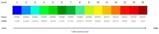
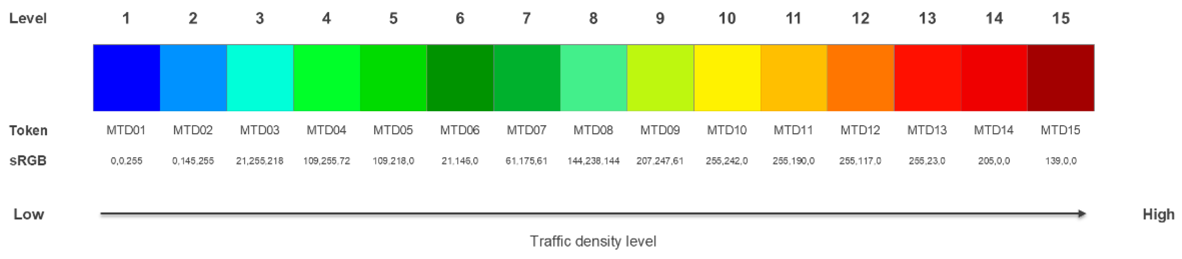
Marine traffic density is portrayed in color by classifying the trafficDensity value of each cell into 15 levels. The color tokens MTD01 to MTD15 are applied to the levels; low density is shown in blue, and as the value increases the color changes through green, yellow, and orange to red. The Lua portrayal rule identifies the interval to which the trafficDensity value belongs, selects the corresponding color, and fills the cell area. In this way, areas where marine traffic is concentrated and areas with relatively low traffic are distinguished by color, and the spatial distribution of traffic density can be seen intuitively. Table 8 lists the AIS sample count interval and color for each level, and Figure 5 shows the color legend. The intervals are based on the 2022–2023 data applied in Section 4.

Table 8. The 15 color levels of marine traffic density.

Level	AIS Sample Count	Color Token	RGB	Meaning
1	1	MTD01	0, 0, 255	Blue, low density
2	2–3	MTD02	0, 145, 255	Sky blue
3	4–8	MTD03	21, 255, 218	Cyan
4	9–17	MTD04	109, 255, 72	Light green
5	18–36	MTD05	109, 218, 0	Green
6	37–76	MTD06	21, 146, 0	Dark green
7	77–157	MTD07	61, 175, 61	Green
8	158–324	MTD08	144, 238, 144	Pale green
9	325–668	MTD09	207, 247, 61	Yellow-green
10	669–1378	MTD10	255, 242, 0	Yellow
11	1379–2840	MTD11	255, 190, 0	Amber
12	2841–5852	MTD12	255, 117, 0	Orange
13	5853–12,059	MTD13	255, 23, 0	Red
14	12,060–24,848	MTD14	205, 0, 0	Dark red
15	24,849–51,198	MTD15	139, 0, 0	Deep red, high density

Figure 5. Color legend for the 15 levels of marine traffic density.

The class boundaries are calculated with the log-binning method of [19]:

$$L_{min} = {\mathrm{l}\mathrm{o}\mathrm{g}}_{10}\left(C_{min}\right), L_{max} = {\mathrm{l}\mathrm{o}\mathrm{g}}_{10}\left(C_{max}\right)$$

(4)

$$L_i = L_{min} + {\displaystyle \frac{i}{n}}\left(L_{max} - L_{min}\right) \mathrm{f}\mathrm{o}\mathrm{r} i = 0, 1, \dots , n$$

(5)

$${Bins}_i = \left[{10}^{L_i}, {10}^{L_{i+1}}\right)$$

(6)

where C_min and C_max are the minimum and maximum AIS sample counts per cell (1 and 51,198 in this dataset), L_min and L_max are their logarithmic values, n = 15 is the number of bins, L_i is the i-th boundary on the logarithmic scale, and Bins_i is the i-th bin on the original scale. In this study, the boundary values were rounded to integers, duplicate boundaries after rounding are kept only once, and the maximum value is assigned to the highest level. Because the boundaries depend on the minimum and maximum of each dataset, the levels are relative within a dataset and show the traffic distribution of the sea area and period concerned; the 16 boundary values and the number of cells per level are recorded as metadata of each dataset (Section 3.5). Logarithmic intervals are used because the sample counts range widely and most cells have low values, so that differences among both low and high values remain visible. The color progression from blue to red follows [19]. The density rule assigns colors only to the intervals of levels 1–15, so cells with the fill value are not painted.

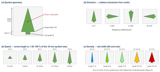
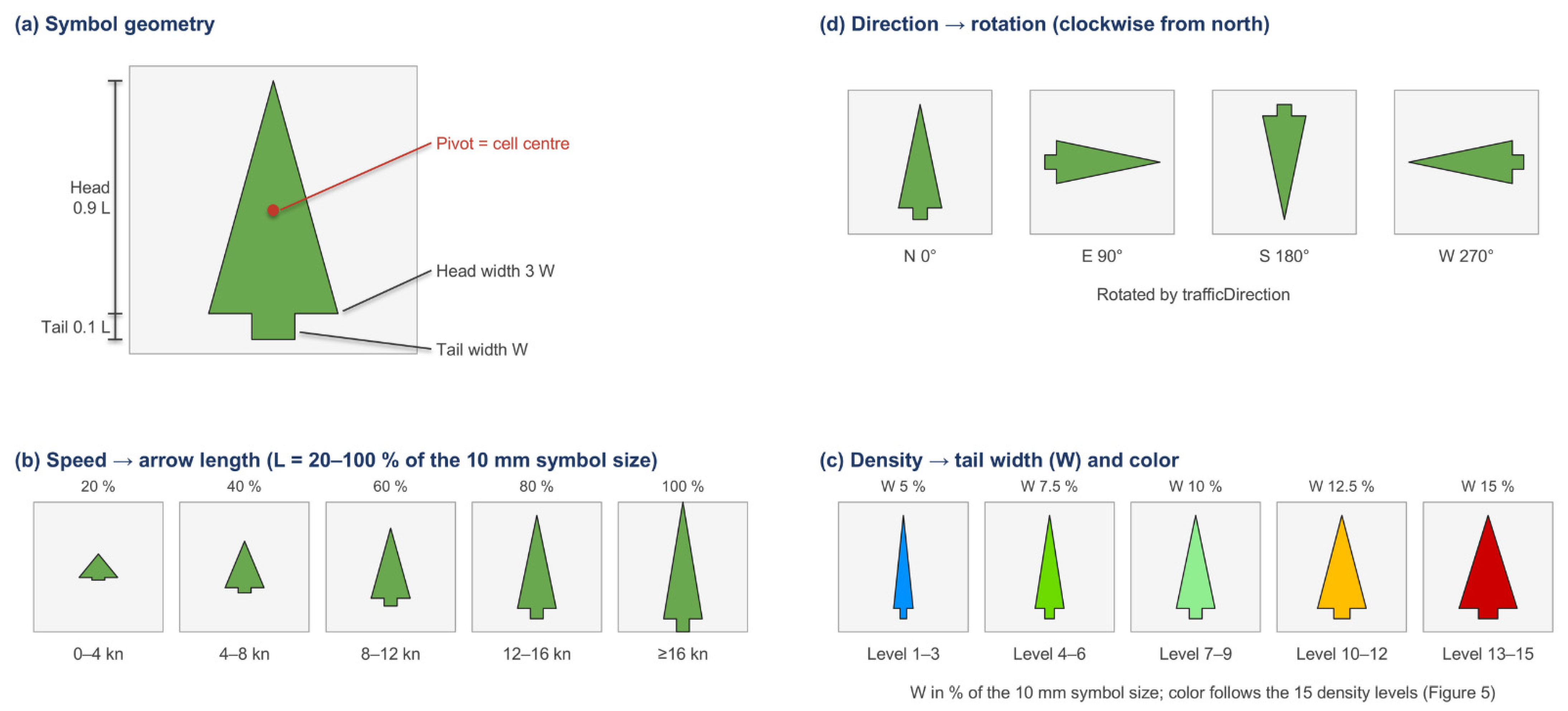
Marine traffic flow is portrayed as arrows by combining the trafficSpeed, trafficDensityDimension, and trafficDirection attributes. trafficSpeed is divided into 5 levels so that the arrow becomes longer as speed increases, and trafficDensityDimension determines the color and width of the arrow according to its level from 1 to 15. As the density level increases, the color changes from blue to red and the width of the arrow increases in steps. The selected arrow is then rotated in the geographic coordinate reference system using the trafficDirection value to indicate the actual direction of traffic flow. The combination of 5 speed levels and 15 density levels gives a total of 75 arrow symbols, so that the speed, density level, and direction of movement of marine traffic are represented together in a single portrayal. Table 9 lists the arrow length for each speed level and Table 10 the color and width for each density level, and Figure 6 shows the design principle of the arrow symbol. The speed classes and the grouping of the 15 density levels into five width categories follow [19], in which speed was divided into five classes reflecting practical navigation characteristics and the density levels were grouped for readability. Each symbol is defined in a 10 mm × 10 mm area on screen and consists of a head (0.9 of the length) and a tail (0.1 of the length); the length increases by 20% of the symbol size for each speed class (20–100%) and the tail width by 2.5% for each density category (5–15%), so that the classes are evenly distinguishable. These dimensions were determined empirically by inspecting the display and were not quantitatively optimized. The flow rule selects no symbol unless the density level is an integer from 1 to 15, so cells with the fill value are not drawn.

Table 9. Arrow length by speed level.

Speed Level	trafficSpeed Range (kn)	Symbol Code	Arrow Length Ratio (of the 10 mm Symbol Size)
1	0 ≤ v < 4	MTF01	20%
2	4 ≤ v < 8	MTF02	40%
3	8 ≤ v < 12	MTF03	60%
4	12 ≤ v < 16	MTF04	80%
5	16 ≤ v	MTF05	100%

Table 10. Arrow color and width by trafficDensityDimension level.

Density Dimension Level	Color	Arrow Tail Width	Description
1–3	MTD01–MTD03	5% of symbol size	Low
4–6	MTD04–MTD06	7.5% of symbol size	Low to medium
7–9	MTD07–MTD09	10% of symbol size	Medium
10–12	MTD10–MTD12	12.5% of symbol size	High
13–15	MTD13–MTD15	15% of symbol size	Very high

Figure 6. Arrow symbol for marine traffic flow and its design principle.

When the display is zoomed out, the arrows of adjacent cells may overlap. Thinning is performed by the display system rather than by the Portrayal Catalogue; the simulator used in this study (Section 4.4) applies the rule of S-111 [12] (Clause 9.3.2 and Annex H-5). With D (mm) as the displayed diagonal of a cell and H_max (mm) as the length of the longest arrow in the display area,

$$m = 1 + \mathrm{fix}\left({\displaystyle \frac{H_{\mathrm{m}\mathrm{a}\mathrm{x}}}{0.5D}}\right)$$

(7)

is calculated, where fix(·) returns the truncated integer value [12], and arrows are drawn only in every mth row and column, always including the row and column of the longest arrow.

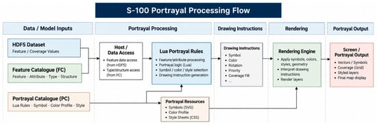
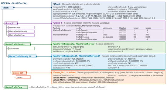
The S-100 portrayal process begins with interpreting the actual values stored in the HDF5 dataset and the data structure defined in the Feature Catalogue (FC). The Lua portrayal rules in the Portrayal Catalogue (PC) are then applied to determine the portrayal appropriate to each feature and attribute value, such as the symbol, color, rotation, drawing priority, and coverage fill. The results are generated as drawing instructions, and the rendering engine applies these instructions together with portrayal resources such as SVG symbols, the color profile, and styles to compose the final screen. Figure 7 shows this process.

Figure 7. S-100 Portrayal Catalogue processing flow.

3.5. HDF5 Encoding

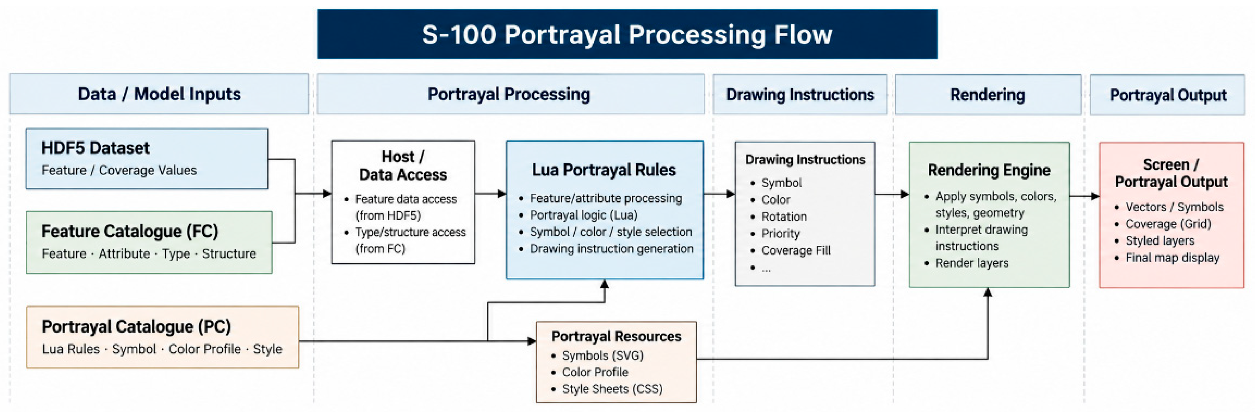
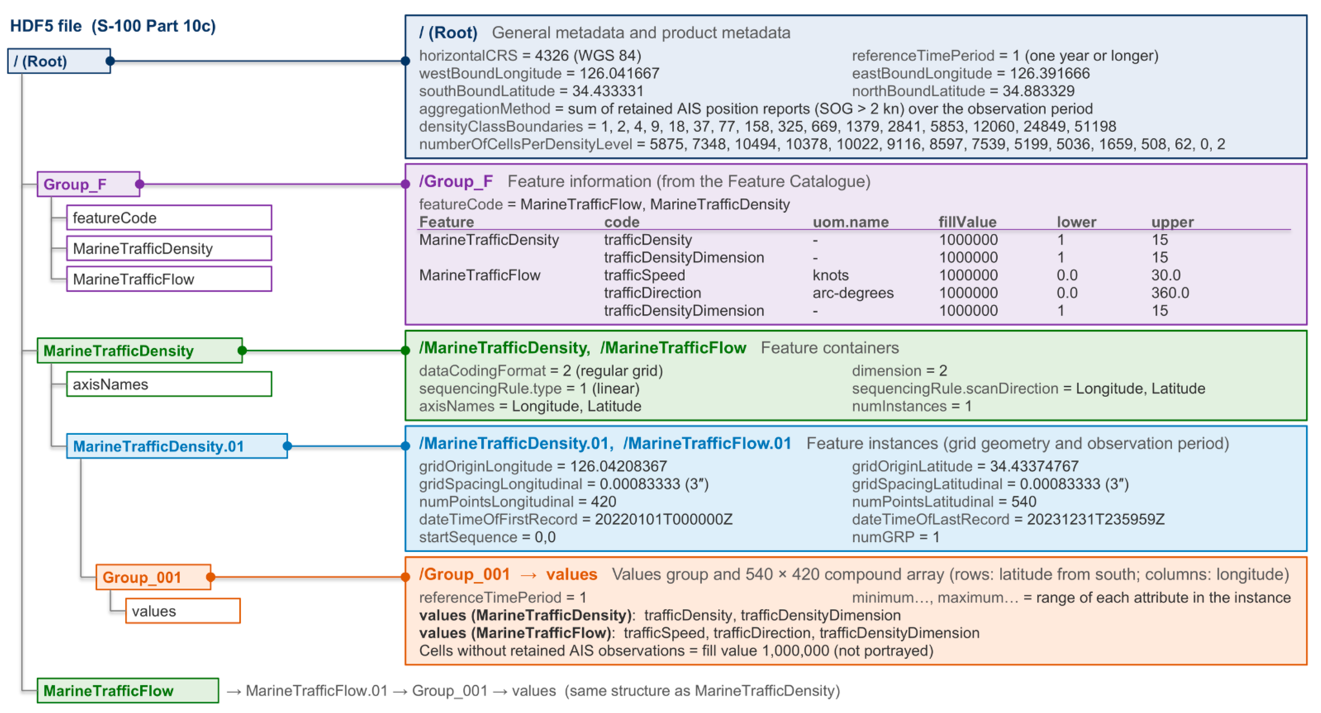
As described in Section 2.2, S-100 Part 10c defines how gridded data are encoded in HDF5. In the proposed model, marine traffic information is organized as a regular grid coverage, the WGS 84 coordinate reference system is applied, and the data are encoded in the HDF5 format. Within the HDF5 file, the structure of the features and attributes is defined in Group_F, and the actual gridded data are stored in the MarineTrafficDensity and MarineTrafficFlow groups. The density data consist of trafficDensity and trafficDensityDimension, and the flow data consist of trafficSpeed, trafficDirection, and trafficDensityDimension. A fill value is applied to cells without data to distinguish actual data from missing areas. Figure 8 shows the HDF5 structure of the proposed model.

Figure 8. HDF5 structure of the proposed model and selected attributes of the dataset produced in this study.

The HDF5 encoding process begins with preprocessing the source marine traffic data and mapping them to the grid of the study area. The preprocessed data are organized for each cell into attribute values such as traffic density, traffic speed, direction of movement, and density level. Metadata such as the coordinate reference system, spatial extent, and product information are then defined in the root group of the HDF5 file, and the name, data type, unit, permitted range, and fill value of the attributes used by each feature are set in Group_F. Next, a group is created for each of the MarineTrafficDensity and MarineTrafficFlow features, and information such as the grid origin coordinates, grid spacing, number of grid points, and spatial extent is specified. Finally, the actual attribute values for each cell are stored in the Group_001/values dataset to produce the HDF5 file.

The grid origin (gridOriginLatitude, gridOriginLongitude) of each feature instance is the center of the first cell at the southwest corner, 34.433748° N, 126.042084° E, and the grid spacing is 0.00083333° in both latitude and longitude. The value array is stored starting from the southernmost row, with 540 rows in latitude and 420 columns in longitude, and the axis names are in the order Longitude, Latitude; the center of the cell in row i and column j is therefore

$${\phi }_i = {\phi }_0 + i\mathsf{\Delta }, {\lambda }_j = {\lambda }_0 + j\mathsf{\Delta } \left(i = 0, \dots , 539; j = 0, \dots , 419\right)$$

(8)

where Δ is the grid spacing. The bounding box of the dataset is defined by the outer edges of the cells (34.433331–34.883329° N, 126.041667–126.391666° E). The reference time period is stored as the referenceTimePeriod attribute of the root group and of each values group (Group_001). The observation period is recorded in UTC in each feature instance group with the same attributes as S-111 [12], dateTimeOfFirstRecord and dateTimeOfLastRecord, and the aggregation method (sum) is recorded as the aggregationMethod attribute of the root group. The 16 density class boundaries and the number of cells per level are recorded in the root group as densityClassBoundaries and numberOfCellsPerDensityLevel. Features are identified by featureCode in Group_F and by the feature groups MarineTrafficDensity and MarineTrafficFlow. Representative values for the dataset of this study are shown in Figure 8 and Table 11.

Table 11. Specifications of the dataset.

Item	Description
Study area	Coastal waters of Mokpo, 34.4333–34.8833° N, 126.0417–126.3917° E
Coordinate reference system	WGS 84 (EPSG:4326)
Data period	1 January 2022–31 December 2023 (UTC); dateTimeOfFirstRecord 20220101T000000Z, dateTimeOfLastRecord 20231231T235959Z
AIS data	Ministry of Oceans and Fisheries; 43,884,996 records (4752 vessels); 16,441,789 records (4268 vessels) used after excluding records at or below 2 kn
Aggregation	Sum of AIS samples per cell over the observation period (aggregationMethod)
Grid spacing	0.00083333° (3″; about 92.6 m north–south, 76.2 m east–west)
Grid origin and order	34.433748° N, 126.042084° E (center of the southwest cell); axis order Longitude, Latitude; rows stored from the south
Number of cells	540 (latitude) × 420 (longitude) = 226,800
Cells with values	81,835 (about 36%)
Fill cells	144,965 (land 106,871; water 38,094, of which 36,938 without AIS reports and 1156 with only reports at or below 2 kn)
Fill value	1,000,000
Density level	1–15; class boundaries 1, 2, 4, 9, 18, 37, 77, 158, 325, 669, 1379, 2841, 5853, 12,060, 24,849, 51,198 (densityClassBoundaries)
Flow speed	2.1–30.0 kn (460 cells stored as 30 kn)
Flow direction	Central values of 36 intervals (5–355°)
Reference time period	1 (one year or longer)
File	HDF5, 828,675 bytes

4. Results

4.1. Study Area and Dataset

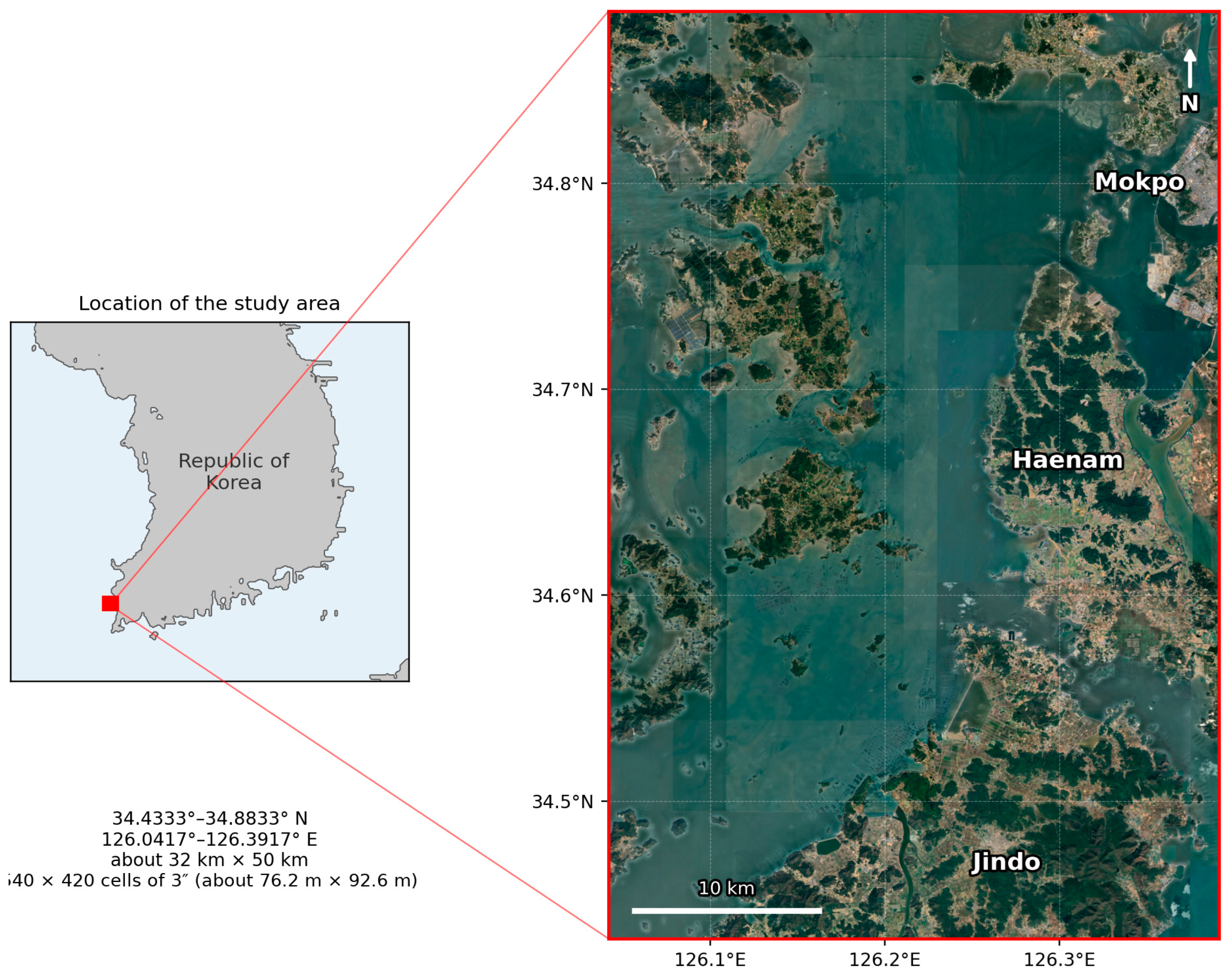
The study area is the coastal waters of Mokpo on the southwestern coast of the Republic of Korea (Figure 9). In this area, the coastal routes of the southern Yellow Sea meet the routes connecting the island region; ships entering and leaving Mokpo Port and Mokpo New Port, passenger ships, and fishing vessels operate together, and traffic is concentrated in the port approach channels and narrow waterways [19]. The dataset covers 34.4333–34.8833° N and 126.0417–126.3917° E.

Figure 9. Study area: coastal waters of Mokpo.

The dataset was built from the results obtained by applying AIS data from 1 January 2022 to 31 December 2023 (UTC). The vessel track data preprocessed in [19] contained 43,884,996 records from 4752 vessels (unique MMSIs; 3610 in 2022 and 3409 in 2023), and no record had a missing position, speed, or course. After the records at or below 2 kn were excluded, 16,441,789 records (37.5%) from 4268 vessels were used. The data contain no vessel type field, so vessel types were not distinguished. The grid spacing is 0.00083333° (3″) in both latitude and longitude, corresponding to about 92.6 m north–south and 76.2 m east–west, and the grid has 540 points in latitude and 420 in longitude, for a total of 226,800 cells. Of these, 81,835 cells, about 36% of the total, contained retained AIS observations and have values, and the fill value was recorded in the remaining 144,965 cells. According to a land–water mask of the same grid, 106,871 of the fill cells are land cells and 38,094 are water cells; of the water cells, 36,938 had no AIS reports and 1156 had only reports at or below 2 kn. The density level is defined as 1–15, the flow speed ranged from 2.1 to 30.0 kn, and the direction was obtained as the central values of 36 intervals of 10° (5°, 15°, …, 355°). The reference time period was recorded as 1 (accumulation over one year or longer), and the values are the totals of the AIS samples over the two years, not annual averages. Table 11 summarizes the main specifications of the dataset.

To keep the dataset identical to the results of [19], the preprocessing of [19] was applied without change, and duplicate reports and AIS “not available” values were not removed separately. Among the retained samples, duplicate reports accounted for 1.73%, speeds of 102.3 kn (speed not available) for 0.56%, and courses of 360° (course not available) for 0.57%. When these records were removed and the data were re-aggregated with the same class boundaries, the density level changed in 1.8% of the cells with values, the flow speed class in 1.4%, and the dominant direction in 1.8%; the number of cells with mean speeds of 30 kn or more decreased from 460 to 421. The reporting intervals were neither harmonized nor interpolated; the median interval between consecutive retained reports of the same vessel within 10 min was 10 s (interquartile range 6–11 s).

Because the AIS sample count is not equivalent to the number of vessel passages (Section 3.1), passage counts were calculated separately for comparison. A run of consecutive reports from the same vessel in the same cell was counted as one passage, and a gap of more than 10 min between reports started a new passage. The 16,441,789 retained samples corresponded to 8,805,580 passages, or 1.87 samples per passage on average (median per cell 1.67). The number of samples per passage depended on the time spent in the cell and on the reporting interval: 3.43 in cells with a mean speed of 2–4 kn, 2.27 for 4–8 kn, 1.82 for 8–12 kn, 1.76 for 12–16 kn, and 3.82 for 16 kn or more. Nevertheless, the Spearman rank correlation between the sample count and the passage count per cell was 0.987, and when both were classified into 15 levels by the same method, 90.4% of the cells agreed within one level. The sample count therefore represents the relative passage frequency well, although it is not a count of passages.

To examine the effect of the 2 kn threshold, the data were also aggregated with thresholds of 1 and 3 kn, with the class boundaries recalculated for each threshold. Samples above 1 kn and at or below 2 kn numbered 546,894, which is 3.3% of the samples retained with 2 kn. With 1 kn, the number of cells with values increased by 542 and the density level changed in 8.4% of the cells with values in both aggregations; with 3 kn, the number of samples decreased by 2.7%, the number of cells with values decreased by 548, and the level changed in 6.6% of the cells. Some slow-moving vessels in port approaches or during maneuvering may therefore be excluded by the threshold (Section 5).

4.2. Dataset Construction

The dataset was built using the output file of the traffic model as input. For each cell, the output file records the grid number, the latitude and longitude extent and center coordinates, the AIS sample count, the interval number of the dominant direction, and the average speed. First, the grid numbers were converted to rows and columns of the 540 × 420 grid, and the result was compared with the positions calculated from the cell center coordinates to confirm that the positions of all cells matched. Next, each value was converted to match the attributes of the Feature Catalogue. The AIS sample count was divided into logarithmic intervals and converted to a 15-level density level, which was recorded in both trafficDensity and trafficDensityDimension. The dominant direction was recorded in trafficDirection after the interval number at 10° spacing was converted to the central angle of the interval, and the average speed was recorded as 30 kn where it was 30 kn or more, in accordance with the value range of the Feature Catalogue (0–30 kn). This applied to 460 cells, or 0.6% of the cells with values; their original values were 30.0 kn or more (median 36.3 kn). Because all speeds of 16 kn or more are portrayed with the same arrow length (Table 9), this truncation does not change the portrayal. However, the numerical values above 30 kn are not retained in the dataset for these cells, whereas the original values remain in the output of the traffic model.

The converted values were stored in an HDF5 file according to the structure described in Section 3.5. In addition to the dataset extent and coordinate reference system, the issue date and the name of the source output file were recorded in the root group, together with the aggregation method, the density class boundaries, and the number of cells per level, and the observation period was recorded in each feature instance group (Section 3.5). Because the values are aggregated per cell, the grid origin of each feature instance was set to the center of the first cell at the southwest corner, and the value arrays were stored starting from the southernmost row. A fill value of 1,000,000 was recorded for all attributes in cells without retained AIS observations. Finally, the value fields of the two features and the attribute codes in Group_F were confirmed to match the attribute bindings of the Feature Catalogue. The values of all five attributes stored in the HDF5 file agreed with those calculated from the model output in all 81,835 cells with values, trafficDensity and trafficDensityDimension were identical in all of these cells, and the fill value was recorded for all attributes in the 144,965 fill cells, with no fill value or NaN in cells with values. The file also passed 12 checks of the required groups and attributes, grid definition, discretization of direction values, speed upper limit, and value ranges.

4.3. Visualization of Traffic Density

To confirm that the density feature is also interpreted in a third-party S-100 display environment, the NIWC S100Viewer (Version 2.1.0.0), developed by the Naval Information Warfare Center Atlantic, which is available from the IHO Geospatial Information Registry, was used [31]. This viewer is test software that supports the visualization of S-100 products; in this study, the Feature Catalogue, the Portrayal Catalogue, and the HDF5 dataset built in Section 4.2 were loaded to display the density feature. In the viewer, the density feature was displayed without any additional settings simply by loading the Feature Catalogue, Portrayal Catalogue, and dataset files.

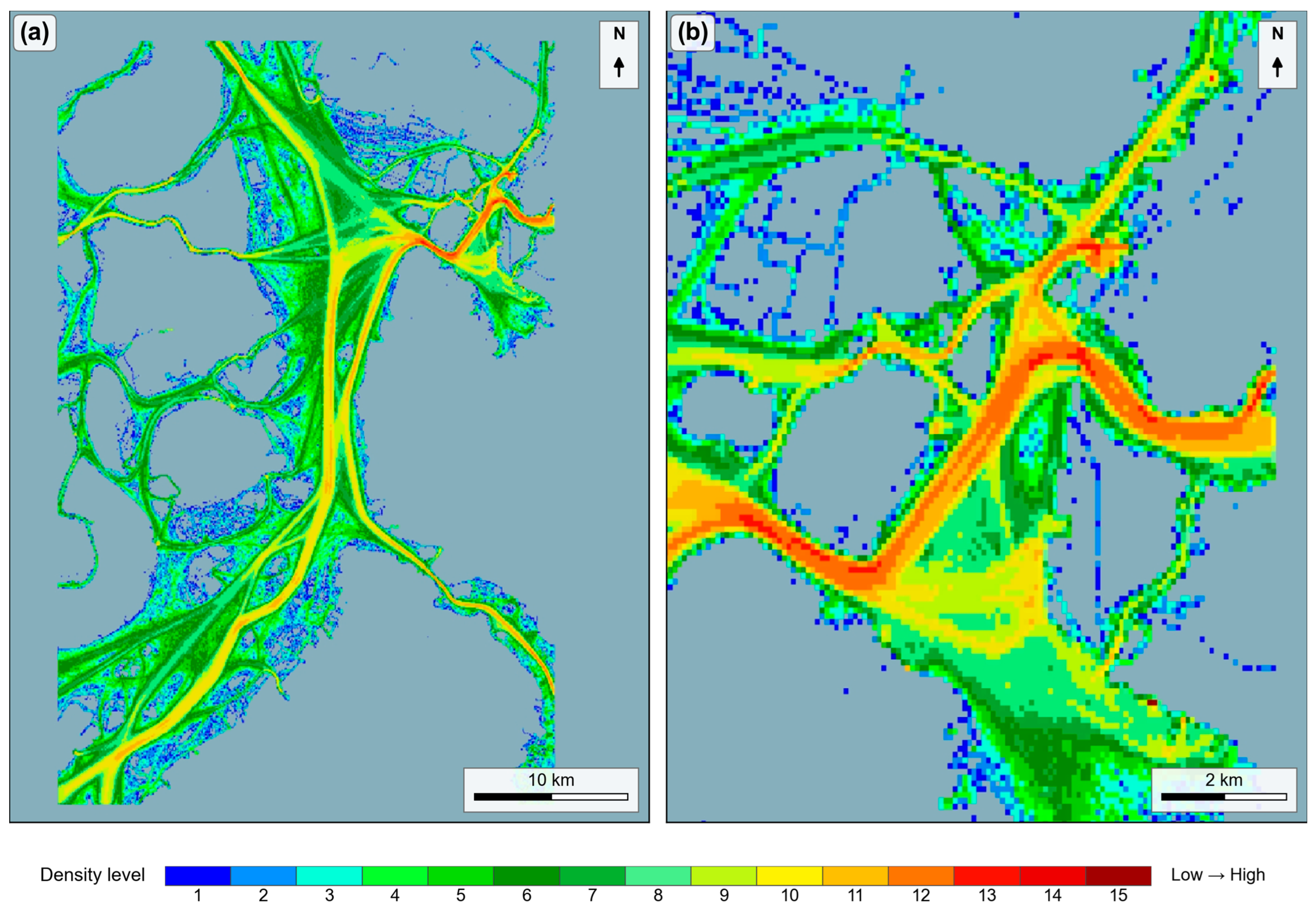
The density feature was displayed without errors, and each cell was filled with one of the 15 color levels according to the portrayal rules in Section 3.4 (Figure 10). To check the display quantitatively, the screenshot of Figure 10b (display scale 1:55,000) and a further enlarged screenshot (1:27,500) were registered to the grid, and the displayed color of each cell was compared with the color of its level; in the whole-area view (Figure 10a, 1:220,000), a cell occupies only about one pixel on the screen, so the cell-by-cell comparison was made on the enlarged views. All cells with values in the two screenshots (7808 and 2708 cells) were displayed in the color of their level, and none of the fill cells (9972 and 1982 cells) were painted. Of the cells with values, levels 1–5 accounted for 53.9% and levels 6–10 for 43.4%, whereas levels 11–15 accounted for 2.7% and appeared only along the main routes and the approach channel to Mokpo Port. Over the whole area (Figure 10a), density appeared continuously along the coastal routes and the routes between islands, and in the enlarged view of the narrow channel near Mokpo Bridge (Figure 10b), high-level cells appeared continuously along the route to and from Mokpo Port. This result shows that a third-party viewer in which no dedicated display function was implemented can interpret and display traffic density data using only the Feature Catalogue and the Portrayal Catalogue.

Figure 10. Marine traffic density displayed in the NIWC S100Viewer: (a) whole area (display scale 1:220,000); (b) enlarged view of the narrow channel near Mokpo Bridge (display scale 1:55,000). The colors correspond to the 15 density levels (Table 8).

4.4. Visualization of Traffic Flow

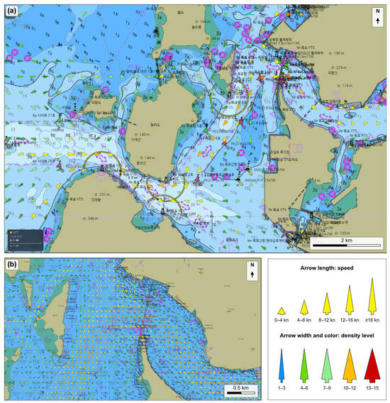
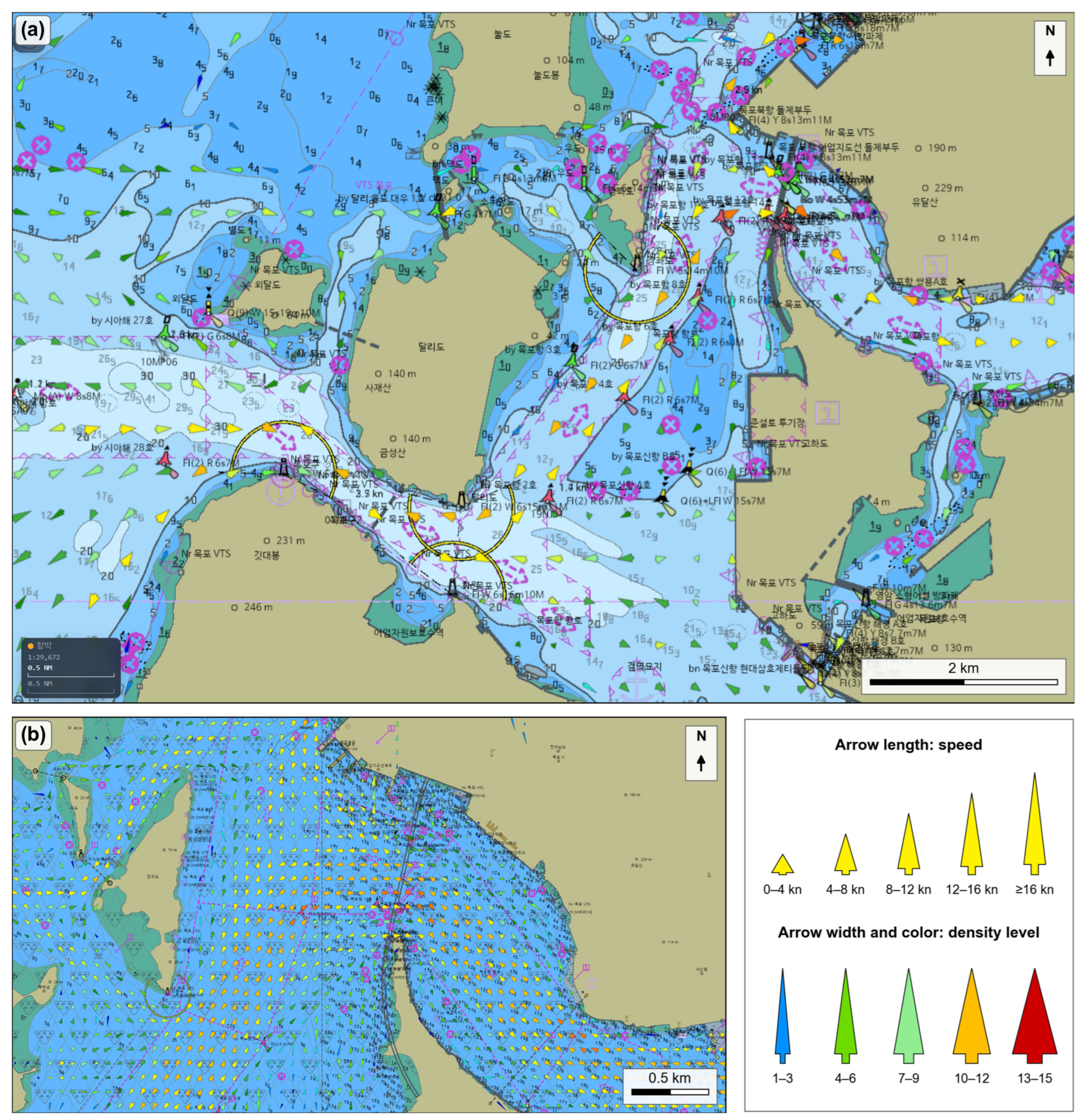
The flow feature was not displayed in the NIWC S100Viewer. The viewer supports coverage portrayal in which grid cells are colored according to their values, as in S-102, but not Lua-based portrayal in which a symbol is determined dynamically for each grid cell, as required for S-111-type arrows. At the time of this study, the Portrayal Catalogue of S-102 Edition 3.0.0 in the IHO GI Registry was provided in Lua, whereas only XSLT-based portrayal rules were found for S-111 Edition 2.0.0. The flow was therefore not displayed because of the implemented scope of the viewer rather than a failure to read the HDF5 data, which were displayed for the density feature. The flow feature was examined in a simulator based on an in-house S-100 chart engine, Naru (Version 1.0.0). The simulator loads the Feature Catalogue, the Portrayal Catalogue, and the dataset in the S-100 manner and reads the Lua portrayal rules and SVG symbols without modification to generate drawing instructions; the processing of dynamic symbols for grid cells is a general function of the engine for S-111-type gridded data, and no modification was made for this product. Because the flow was verified only in this simulator, its display in an independent S-100 viewer has not yet been demonstrated.

In accordance with the portrayal rules, one of the 75 symbols was selected for each cell from the combination of speed and density level, and the symbol was displayed rotated relative to true north according to the trafficDirection value (Figure 11). Flow speeds of 8–12 kn were the most frequent at 47.1%, followed by 4–8 kn at 23.5%, 12–16 kn at 15.2%, 16 kn or more at 7.8%, and less than 4 kn at 6.4%, so that all 5 levels of arrow length were used. The flow layer could be overlaid on the ENC and the density layer, and the two types of information could be viewed together by adjusting the transparency of the layers. In the approach channel into Mokpo Port (Figure 11a) and in the further enlarged view near Mokpo Bridge (Figure 11b), the arrows were aligned with the direction of the routes, and differences in speed and density between cells could be distinguished from the length, width, and color of the symbols.

Figure 11. Marine traffic flow displayed in the simulator based on the S-100 chart engine Naru: (a) approach channel to Mokpo Port (display scale 1:29,672); (b) enlarged view near Mokpo Bridge. The legend shows the arrow length by speed and the arrow width and color by density level (Figure 6). The direction of each arrow represents only the dominant direction of the cell, whereas its width and color represent the density level calculated from the observations in all directions. The Korean labels in the background are the place names and aids-to-navigation names of the ENC.

The Lua portrayal rules were also executed as they are with test data of known values, using Lua (Version 5.5) through lupa (Version 2.8). For all 990 combinations of 11 speed values (0, 2.1, 3.99, 4, 7.99, 8, 11.99, 12, 15.99, 16, and 30 kn), the 15 density levels, and six directions (0°, 5°, 95°, 185°, 275°, and 355°), the expected symbol was selected, all 75 symbols were used, and the rotation was instructed as the trafficDirection value clockwise from true north in the geographic coordinate reference system. For the fill value, out-of-range levels (0 and 16), a non-integer level, and a negative speed, no symbol was drawn. In the density rule, each level from 1 to 15 corresponded to exactly one color token (MTD01–MTD15), and the fill value to none. The same results were obtained when the density levels were given as integers.

Because the flow symbol shows only the dominant direction, the distribution of directions in each cell was also examined. The share of samples in the dominant 10° sector had a median of 33.3% per cell, and 51.1% when the two adjacent sectors (±10°) were included. When the samples were summed over 30° windows, 62.2% of the 25,407 cells with 100 or more samples had a second peak with at least half the samples of the first peak at 150° or more from it (two-way traffic), and 2.8% had such a peak 45–150° from it (crossing traffic). For example, in a two-way cell at 34.783° N, 126.387° E (7183 samples), 46% of the samples were within ±10° of the stored direction of 205° and 41% within ±10° of the opposite direction of 25°; in a crossing cell at 34.755° N, 126.322° E (1758 samples), 46% were within ±10° of the stored direction of 285° and 29% within ±10° of 55°. In such cells, the arrow represents only the most frequent direction; the arrow does not represent the opposite or crossing traffic, although this traffic is included in the density level.

4.5. Summary of Results

The results of Section 4 are summarized as follows. First, the 2022–2023 output of the traffic model was converted into an HDF5 dataset with the S-100 Part 10c structure, and density and flow values were recorded in 81,835 cells of the 540 × 420 grid. In the conversion, the positions of all cells matched the grid numbers, and the value fields of the two features matched the attribute bindings of the Feature Catalogue, and the stored values agreed with the model output in all cells. Second, the density feature was displayed in 15 color levels in the third-party NIWC S100Viewer using only the Feature Catalogue, the Portrayal Catalogue, and the dataset; every cell with a value in the compared screenshots was displayed in the color of its level, and the high-level cells were concentrated along the main routes and the approach channel to Mokpo Port. Third, the flow feature was not displayed in the NIWC S100Viewer, but in the simulator, which reads the Portrayal Catalogue without modification, it was displayed with the 75 symbols determined by speed and density level, and the symbols were rotated according to the dominant direction and aligned with the direction of the routes; the Lua rules selected the expected symbol in all 990 test combinations, but the display of the flow in an independent S-100 viewer has not yet been demonstrated. These results show that historical marine traffic information can be defined, encoded, and portrayed as S-100 gridded data according to the rules of its Portrayal Catalogue. Table 12 summarizes the validation items and results.

Table 12. Validation items and results.

Item	Method	Result
Feature Catalogue	Validation against the S100FC schema (XSD).	Valid.
HDF5 structure and metadata	12 checks: required groups and attributes, grid definition, discretization of directions, speed upper limit, value ranges.	12 of 12 passed.
Spatial registration	Rows and columns from the grid numbers compared with those from the cell-center coordinates.	Agreed in all 81,835 cells.
Value preservation	Values from the model output compared with the values stored in HDF5 (five attributes).	Agreed in all 81,835 cells.
Density attributes	trafficDensity compared with trafficDensityDimension.	Identical in all 81,835 cells.
Fill value	Fill value in cells without retained AIS observations.	Recorded for all attributes in 144,965 cells; none in cells with values.
Flow portrayal rule	Lua rule executed for 990 combinations (11 speeds × 15 levels × 6 directions) and 6 invalid inputs.	Expected symbol in 990 of 990; all 75 symbols used; rotation by trafficDirection; no symbol for invalid inputs.
Density portrayal rule	Lua rule executed for levels 1–15 and the fill value.	One color token per level (MTD01–MTD15); fill value not painted.
Density display	NIWC S100Viewer (Version 2.1.0.0); screenshots at 1:55,000 (Figure 10b) and 1:27,500 registered to the grid.	All 7808 and 2708 cells with values in the color of their level; no fill cell painted.
Flow display	Simulator based on Naru (Version 1.0.0); NIWC S100Viewer.	Displayed in the simulator; not displayed in NIWC S100Viewer.

Table 12. Validation items and results.

Item	Method	Result
Feature Catalogue	Validation against the S100FC schema (XSD).	Valid.
HDF5 structure and metadata	12 checks: required groups and attributes, grid definition, discretization of directions, speed upper limit, value ranges.	12 of 12 passed.
Spatial registration	Rows and columns from the grid numbers compared with those from the cell-center coordinates.	Agreed in all 81,835 cells.
Value preservation	Values from the model output compared with the values stored in HDF5 (five attributes).	Agreed in all 81,835 cells.
Density attributes	trafficDensity compared with trafficDensityDimension.	Identical in all 81,835 cells.
Fill value	Fill value in cells without retained AIS observations.	Recorded for all attributes in 144,965 cells; none in cells with values.
Flow portrayal rule	Lua rule executed for 990 combinations (11 speeds × 15 levels × 6 directions) and 6 invalid inputs.	Expected symbol in 990 of 990; all 75 symbols used; rotation by trafficDirection; no symbol for invalid inputs.
Density portrayal rule	Lua rule executed for levels 1–15 and the fill value.	One color token per level (MTD01–MTD15); fill value not painted.
Density display	NIWC S100Viewer (Version 2.1.0.0); screenshots at 1:55,000 (Figure 10b) and 1:27,500 registered to the grid.	All 7808 and 2708 cells with values in the color of their level; no fill cell painted.
Flow display	Simulator based on Naru (Version 1.0.0); NIWC S100Viewer.	Displayed in the simulator; not displayed in NIWC S100Viewer.

5. Discussion & Conclusions

Compared with existing marine traffic information and the traffic-related S-100 products, the proposed model has the following features (Table 13). First, the nature of the information differs. S-127 and S-212 handle management and instruction information, such as traffic management areas and rules and ship-specific traffic clearance and anchorage assignment, in vector form [15,16], whereas the proposed model handles, on a grid, the density and flow obtained by accumulating AIS data over a given period for each cell. This defines as S-100 data the information corresponding to the gap in the type of information (G1) identified in Section 2.3. Second, the attributes and display methods of marine traffic information were defined in machine-readable specifications. The outputs of existing studies and services differ in grid system and classification criteria and were provided as maps or images [4,5,6,7]; in the proposed model, the meaning, units, and value ranges of the density level, speed, and direction are defined in the Feature Catalogue and the display method in the Portrayal Catalogue, and the data are encoded in HDF5 according to S-100 Part 10c. As a result, as shown in Section 4.3, the density was displayed using only the catalogues and the dataset even in a third-party viewer in which no dedicated display function was implemented (G2). Third, portrayal rules that determine a symbol by combining several attributes for each grid cell were implemented. In S-111, the color and size of the current arrow are determined by current speed alone and the arrow is rotated according to the current direction [12], whereas the flow symbol of the proposed model takes its length from speed and its width and color from the density level and is rotated according to the dominant direction, so that three attributes are represented in a single symbol (G3).

Table 13. Comparison of the proposed model with existing traffic-related and gridded S-100 products.

Item	Target Information	Nature of Information	Spatial Representation (Encoding)	Traffic Information (Density and Flow)	Grid Portrayal
S-127 [15]	VTS, pilotage, routing measures, ship reporting	Management and regulatory	Vector (GML)	X	–
S-212 [16]	Traffic clearance, anchorage assignment	Ship-specific clearance messages	Vector (GML)	X	–
S-111 [12]	Surface currents	Natural phenomenon	Grid (HDF5)	X	Arrow: current speed → color and size; current direction → rotation
Proposed model	Marine traffic density and flow	Historical statistics	Grid (HDF5)	O	Density: color by value interval Flow arrow: speed → length; density → width and color; direction → rotation

O: applicable; X: not applicable; –: vector product without grid portrayal.

From the above, the contributions of this study can be summarized as follows. First, marine traffic information was defined as an S-100 data model. Density and flow were separated into two grid features, and an application schema and Feature Catalogue consisting of five attributes, including the density level, speed, direction, and reference time period, were presented. Second, the output of the traffic model was converted into S-100 gridded data, and an HDF5 dataset on a 540 × 420 grid was built from the 2022–2023 data for the coastal waters of Mokpo. Third, portrayal rules that represent density in 15 color levels and flow with 75 rotated symbols determined by speed and density level were implemented in Lua and SVG, thereby portraying a multi-attribute grid. Fourth, the dataset and the catalogues were validated quantitatively (Table 12); the density was displayed according to the defined rules in a third-party viewer, and the flow in a simulator that reads the Portrayal Catalogue without additional feature-specific hard-coding or modification, although the display of the flow in an independent S-100 viewer has not been demonstrated.

The limitations of this study and future work are as follows. First, density was calculated from the number of AIS samples recorded in each cell, which depends on the time spent in the cell and on the reporting interval and is not a count of passages, although it agreed closely with the passage counts (Section 4.1). The size and type of ships were not reflected in the model, because the track data used contain no vessel type or size fields; trafficDensityDimension therefore has the same value as trafficDensity in this dataset. If the model is extended to reflect this information, traffic information by ship type or ship size could also be provided in the same structure. Second, the Feature Catalogue defines a reference time period that distinguishes yearly, monthly, and time-of-day accumulation, but the dataset built in this study covers only yearly accumulation. To provide traffic characteristics by season or time of day, datasets must be built for each reference time period, and the way in which they are selected and displayed on navigation equipment must also be examined; a temporal structure that supports comparisons across years, seasons, and reporting periods is also left for future work. Third, the intervals of the density levels were determined, as in the previous model [19], by dividing the range of AIS sample counts in the target data into 15 intervals on a logarithmic scale. Because the interval boundaries depend on the range of the data, the same level does not represent the same sample count across datasets for different sea areas or periods. The boundaries are therefore recorded in the metadata of each dataset (Section 3.5); to compare datasets for several sea areas directly, fixed interval boundaries would also need to be defined. Fourth, the speed threshold of 2 kn adopted from [19] may exclude some slow-moving vessels in port approaches or during maneuvering (Section 4.1). Fifth, the 3″ grid follows [19] and distinguished the narrow channels of the study area, but the results may depend on the grid size, and smaller grids may be needed for narrower waters. Sixth, the flow is represented by the dominant direction only, so the opposite or crossing traffic in two-way and crossing cells (Section 4.4) is not shown by the arrows; representing several directions in a cell is left for future work. Seventh, the dataset in this study accumulates data from the past 2 years and is not linked to real-time AIS data. Because the model aggregates AIS data per cell and converts them into an HDF5 dataset, it could also be used for up-to-date traffic information if datasets are generated and updated from AIS data received in real time. This, however, requires the additional development of a system that handles data reception, computation, and the distribution and updating of datasets.

In terms of portrayal, the following issues remain. The first is how flow symbols are displayed at different scales. In the simulator, the arrows were thinned when zoomed out according to the rule of S-111 [12] (Section 3.4), so the flow in the omitted cells does not appear on a zoomed-out display. However, whether thinning is appropriate for traffic flow in congested areas, or whether it is better to group several cells and show a representative direction and speed, needs to be compared and examined. The second is readability. The distinguishability of the 75 symbols and 15 colors and the suitability of the information for navigation were not evaluated; an evaluation by users such as navigators and a comparison with simpler visualization methods, such as arrows determined by a single attribute as in S-111, are left for future work. The third is interoperability between products. This study confirmed that the traffic information layers can be overlaid on the ENC, and viewing groups, drawing priorities, and display planes were specified in the Portrayal Catalogue. However, the interoperability rules between products in S-98 were neither applied nor verified [32], so interoperability, including possible conflicts with other navigational information, when the layers are displayed together with other products such as S-101, S-102, and S-111 needs to be examined. In addition, the flow was displayed only in a simulator based on an in-house chart engine; its display in other S-100 viewers remains to be verified as Lua-based Portrayal Catalogues for gridded data are developed by the IHO and the functions of display engines are extended. Finally, developing the proposed model into a formal Product Specification requires preparing the Product Specification documents in accordance with the S-97 guidelines [20], testing interoperability according to S-98, and testing on S-100 ECDIS.

This study defined historical marine traffic information derived from AIS data, namely traffic density and flow, as S-100-based gridded hydrographic information. Based on the output of the previous traffic flow model [19], the requirements were derived; an application schema and Feature Catalogue consisting of two grid features and five attributes and a Portrayal Catalogue consisting of 15 density color levels and 75 flow symbols were designed; and the data were encoded in HDF5 according to S-100 Part 10c. When a dataset on a 540 × 420 grid was built from the 2022–2023 AIS data for the coastal waters of Mokpo, the density was displayed in a third-party viewer using only the catalogues and the dataset, and the flow was displayed in a simulator based on an in-house S-100 chart engine as rotated symbols reflecting speed, density, and direction; the stored values and the portrayal rules were also verified quantitatively.

These results show that historical marine traffic information, which has so far been provided in different formats by individual studies and services, can be defined, encoded, and portrayed as S-100 gridded data in the same framework as gridded hydrographic information such as bathymetry, water level, and surface currents. This study demonstrates this feasibility, but not operational interoperability with S-100 navigation systems or the usefulness of the information for navigation, which remain to be verified. Because both the input data (AIS) and the data model (S-100) are international standards, datasets for other sea areas can be produced with the same procedure wherever AIS data are available; the features, attributes, and encoding structure remain the same, and the class boundaries are calculated for each dataset and recorded in its metadata. If ship size and type, data for each reference time period, and linkage with real-time AIS are incorporated in the future and interoperability with other S-100 products is verified, the proposed model could be developed into a Product Specification for marine traffic information.

References

- Lee, J.-S.; Kim, T.-H.; Park, Y.-G. Maritime Transport Network in Korea: Spatial-Temporal Density and Path Planning. J. Mar. Sci. Eng. 2023, 11, 2364. [Google Scholar] [CrossRef] [Scilit]
- Luong, T.N.; Hwang, S.; Im, N. Harbour Traffic Hazard Map for Real-Time Assessing Waterway Risk Using Marine Traffic Hazard Index. Ocean Eng. 2021, 239, 109884. [Google Scholar] [CrossRef] [Scilit]
- Li, H.; Yang, Z. Incorporation of AIS Data-Based Machine Learning into Unsupervised Route Planning for Maritime Autonomous Surface Ships. Transp. Res. Part E Logist. Transp. Rev. 2023, 176, 103171. [Google Scholar] [CrossRef] [Scilit]
- Kim, H.-S.; Lee, E.; Lee, E.-J.; Hyun, J.-W.; Gong, I.-Y.; Kim, K.; Lee, Y.-S. A Study on Grid-Cell-Type Maritime Traffic Distribution Analysis Based on AIS Data for Establishing a Coastal Maritime Transportation Network. J. Mar. Sci. Eng. 2023, 11, 354. [Google Scholar] [CrossRef] [Scilit]
- Lee, D.; Jang, D.; Yoo, S. Development of a Multidimensional Analysis and Integrated Visualization Method for Maritime Traffic Behaviors Using DBSCAN-Based Dynamic Clustering. Appl. Sci. 2025, 15, 529. [Google Scholar] [CrossRef] [Scilit]
- EMODnet. Human Activities EU Vessel Density Map: Detailed Method (Version 1.5, 2019). Available online: https://emodnet.ec.europa.eu/sites/emodnet.ec.europa.eu/files/public/Vessel%20density%20maps_method_v1.5.pdf (accessed on 26 October 2026).
- HELCOM AIS Shipping Density Maps. Available online: https://metadata.helcom.fi/geonetwork/srv/api/records/2558244b-0cea-46e9-8053-af6ef5d01853 (accessed on 16 October 2026).
- IHO. S-100 Universal Hydrographic Data Model, 5.2.1. ed.; International Hydrographic Organization: Monaco, 2025. [Google Scholar]
- Duan, J.; Wan, X.; Luo, J. A Review of Universal Hydrographic Data Model. Surv. Rev. 2021, 53, 183–191. [Google Scholar] [CrossRef] [Scilit]
- IHO. Bathymetric Surface Product Specification (S-102), 3.0.0. ed.; International Hydrographic Organization: Monaco, 2024. [Google Scholar]
- IHO. Water Level Information for Surface Navigation Product Specification (S-104), 2.0.0. ed.; International Hydrographic Organization: Monaco, 2024. [Google Scholar]
- IHO. Surface Currents Product Specification (S-111), 2.0.0. ed.; International Hydrographic Organization: Monaco, 2024. [Google Scholar]
- IHO. Smart Navigation Moves Closer to Reality: Completion of Phase 1 of the S-100 Implementation. Available online: https://iho.int/en/smart-navigation-moves-closer-to-reality-completion-of-phase-1-of-the-s-100-implementation (accessed on 16 October 2026).
- IMO. Resolution MSC.530(106): Performance Standards for Electronic Chart Display and Information Systems (ECDIS); International Maritime Organization: London, UK, 2022. [Google Scholar]
- IHO. Marine Traffic Management Product Specification (S-127), 1.0.0. ed.; International Hydrographic Organization: Monaco, 2018. [Google Scholar]
- IALA. VTS Digital Information Product Specification (S-212); Draft 0.7.3.; IALA: Saint-Germain-en-Laye, France, 2024. [Google Scholar]
- IALA. Inter-VTS Exchange Format (S-210 IVEF). Available online: https://www.iala.int/technical/data-modelling/iala-s-200-development-status/ (accessed on 16 October 2026).
- IEC 63173-1:2021; Data Interface—S-421 Route Plan Based on S-100 (IEC 63173-1). International Electrotechnical Commission: Geneva, Switzerland, 2021.
- Oh, D.H.; Zhu, F.; Im, N. A High-Resolution Dynamic Marine Traffic Flow Visualization Model Using AIS Data. J. Mar. Sci. Eng. 2025, 13, 1971. [Google Scholar] [CrossRef] [Scilit]
- IHO. Guidelines for Creating S-100 Product Specifications (S-97), 1.1.0. ed.; International Hydrographic Organization: Monaco, 2020. [Google Scholar]
- Wang, Y.; Wen Liu, R.; Liu, J.; Yang, L.; Liu, Y. AIS Data-Driven Maritime Traffic Flow Prediction and Density Visualization Using Multitime Scale Temporal Feature Fusion Network. IEEE Sens. J. 2025, 25, 11357–11365. [Google Scholar] [CrossRef] [Scilit]
- IALA. Guideline 1089 on Provision of Vessel Traffic Services (Types of Service), 1st ed.; IALA: Saint-Germain-en-Laye, France, 2012. [Google Scholar]
- Kim, H.-S.; Cho, D.J.; Lee, E.J.; Park, K.H.; Park, E.B.; Han, J.S.; Baek, J.H. Development and Empirical Validation of a Real-Time AIS-Based Maritime Traffic Visualisation Framework for Shore-Based Remote Control Centres of Maritime Autonomous Surface Ships. J. Mar. Eng. Technol. 2026, 25, 363–378. [Google Scholar] [CrossRef] [Scilit]
- Guo, W.; Zhang, X.; Wang, J.; Feng, H.; Tengecha, N.A. Traffic Organization Service for Maritime Autonomous Surface Ships (MASS) with Different Degrees of Autonomy. J. Mar. Sci. Eng. 2022, 10, 1889. [Google Scholar] [CrossRef] [Scilit]
- Lee, S.; Jeong, H.; Lee, C. Modeling of Historical Marine Casualty on S-100 Electronic Navigational Charts. Appl. Sci. 2025, 15, 6432. [Google Scholar] [CrossRef] [Scilit]
- Luo, J.; Liu, Z.; Tang, H.; Jiao, C.; Geng, X.; Guo, H. A High-Density Bathymetric Data Model and System Construction Approach Integrated with S-100 for Unmanned Surface Vessel Intelligent Navigation. J. Mar. Sci. Eng. 2026, 14, 633. [Google Scholar] [CrossRef] [Scilit]
- Tomczuk, T. The Role of Machine-Readable Portrayal Catalogue for Displaying New S-100 Format Data in ECDIS. TransNav Int. J. Mar. Navig. Saf. Sea Transp. 2025, 19, 1081–1086. [Google Scholar] [CrossRef] [Scilit]
- Lee, S.; Lee, C.; Kim, G.; Na, H.; Kim, H.; Lee, J.; Park, M. A Study of S-100 Based Product Specifications from a Software Implementation Point of View: Focusing on Data Model Representation, Similar Features and Symbols, and ECDIS and VTS Software. J. Navig. 2022, 75, 1226–1242. [Google Scholar] [CrossRef] [Scilit]
- Cho, H.; Lee, C.; Lee, S. Analysis of Security Vulnerabilities in S-100-Based Maritime Navigation Software. Sensors 2026, 26, 1246. [Google Scholar] [CrossRef] [Scilit] [PubMed]
- ISO 19109:2015; Geographic Information—Rules for Application Schema. International Organization for Standardization: Geneva, Switzerland, 2015.
- Naval Information Warfare Center Atlantic, United States Navy NIWC S100Viewer and Shore ECDIS, Version 2.1.0.0. Available online: https://registry.iho.int/repository/list.do (accessed on 16 October 2026).
- IHO. S-100 ECDIS and Interoperability Specification (S-98), 2.0.0. ed.; International Hydrographic Organization: Monaco, 2025. [Google Scholar]
Disclaimer/Publisher’s Note: The statements, opinions and data contained in all publications are solely those of the individual author(s) and contributor(s) and not of MDPI and/or the editor(s). MDPI and/or the editor(s) disclaim responsibility for any injury to people or property resulting from any ideas, methods, instructions or products referred to in the content. |
© 2026 by the authors. Licensee MDPI, Basel, Switzerland. This article is an open access article distributed under the terms and conditions of the Creative Commons Attribution (CC BY) license.