Phononic-Crystal-Inspired Design of a Gradient-Porosity Multi-Row Pile Breakwater for Enhanced Wave Attenuation

Abstract

Inspired by the concepts of phononic crystals and spatially graded wave control, this study proposes a gradient-porosity distributed multi-row pile breakwater (GPDMPB), in which porosity decreases stepwise from 0.30 to 0.10 along the wave-propagation direction. A three-dimensional numerical wave tank was established using OpenFOAM and OlaFlow. Reflection, transmission, and energy dissipation characteristics were evaluated for different porosity distributions, pile-row spacings, and wave steepnesses. Under the investigated regular-wave conditions, compared with the conventional permeable breakwaters considered, the GPDMPB achieved lower reflection and transmission and higher energy dissipation; the conventional configurations exhibited reflection and transmission coefficients 1.16–2.94 and 1.16–3.01 times those of the GPDMPB, while their dissipation coefficients were only 0.35–0.87 times as large. Compared with a uniform-porosity array (P = 0.20) having the same total blockage, the GPDMPB exhibited lower transmission, higher energy dissipation, and generally lower or comparable reflection. Flow-field results revealed successive flow contraction, separation, and recirculation through the pile rows, indicating progressive attenuation through distributed wave–structure interactions. Pile-row spacing mainly affected reflection, whereas increasing wave steepness increased reflection and transmission and reduced dissipation. These results highlight the potential of the proposed spatially graded configuration to improve wave attenuation in multi-row pile breakwaters under the investigated regular-wave conditions.

1. Introduction

The manipulation of wave propagation through artificially structured media has attracted sustained interest in solid mechanics, acoustics, and phononics. Phononic crystals, typically composed of periodically arranged scattering units, provide an effective platform for tailoring acoustic and elastic wave propagation through wave–structure interactions. Their periodic architecture can give rise to multiple scattering, Bragg-type interference, and frequency-dependent transmission characteristics, enabling the regulation of wave propagation, reflection, localization, and attenuation [1,2]. Beyond strictly periodic configurations, spatial modulation of the constituent units provides additional degrees of freedom for controlling wave behavior. In particular, graded phononic crystals and metamaterials, in which geometric or effective properties vary gradually in space, have demonstrated that wave propagation can be manipulated through deliberately designed structural gradients [3,4].

The concepts developed for structured wave-controlling media are not limited to elastic or acoustic waves. Surface water waves can also interact strongly with periodically arranged structures, and analogies between water-wave systems and phononic crystals have motivated extensive studies of artificial structures for manipulating water-wave propagation [5]. Early studies demonstrated that periodic arrays of vertical cylinders can exhibit pronounced multiple-scattering and band-structure effects, with their wave-propagation characteristics strongly influenced by the geometry and filling fraction of the cylinder array [6]. Li and Mei [7] analyzed the resonant response of surface waves interacting with two-dimensional cylinder lattices and interpreted the resulting propagation behavior within a Bragg-resonance framework. These studies indicate that an ordered array of vertical cylindrical elements can serve as a macroscopic structured medium for manipulating surface-wave propagation.

More recently, attention has extended from strictly periodic arrays to spatially graded structures, in which the properties of successive scattering elements vary along the direction of wave propagation. Such grading allows the wave–structure interaction to evolve spatially rather than remaining uniform throughout the array. Bennetts et al. [8], for example, investigated a graded array of C-shaped vertical cylinders and demonstrated that spatial variation in the resonator properties can redistribute water-wave energy along the array. Archer et al. [9] subsequently verified in wave-flume experiments that gradually varying a vertical-cylinder array can redistribute localized wave-energy amplification across a broad range of frequencies. These studies motivate the use of spatial grading as a design concept for water-wave structures. Whether a particular finite pile array exhibits comparable dispersion or resonance characteristics requires separate investigation.

From an engineering perspective, permeable and pile-supported breakwaters offer a natural platform for implementing such structured-array concepts because they consist of discrete elements interacting successively with incident waves. Compared with conventional impermeable breakwaters, permeable structures can maintain water exchange while reducing wave transmission. However, increasing the obstruction of a pile-supported structure to suppress transmitted waves generally tends to increase wave reflection, whereas highly permeable configurations reduce reflection at the expense of increased transmission. Previous studies have therefore attempted to improve the balance among reflection, transmission, and energy dissipation through curved wave-facing surfaces, additional wave screens, perforated components, hollow structures, and composite filling materials [10,11,12,13,14,15]. Although these approaches can improve hydrodynamic performance, they generally rely on additional or increasingly complex structural components. Comparatively limited attention has been paid to regulating wave propagation by modifying the spatial arrangement and porosity distribution of a simple multi-row pile array itself.

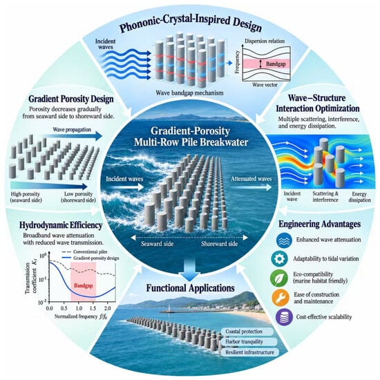
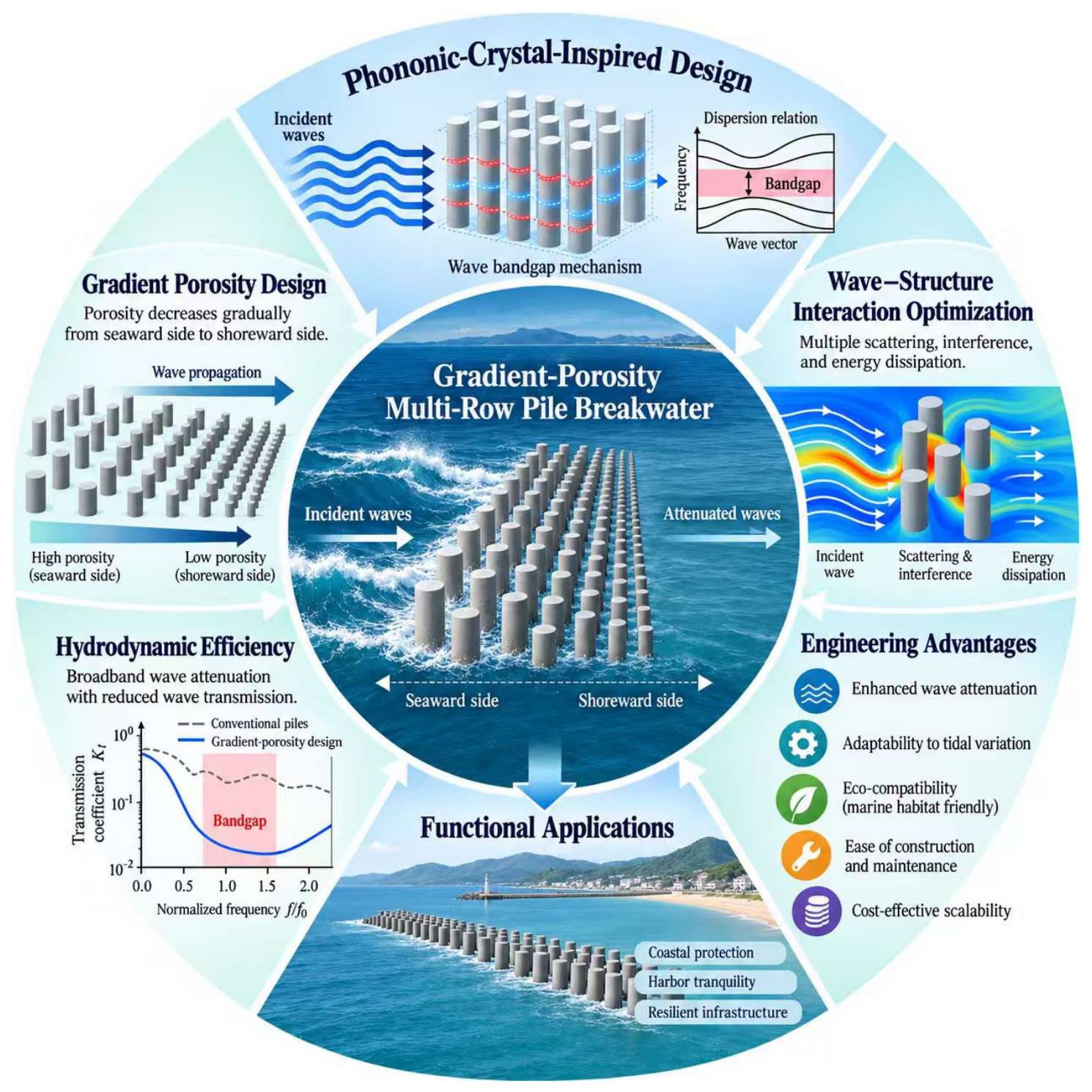
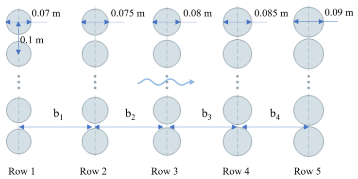
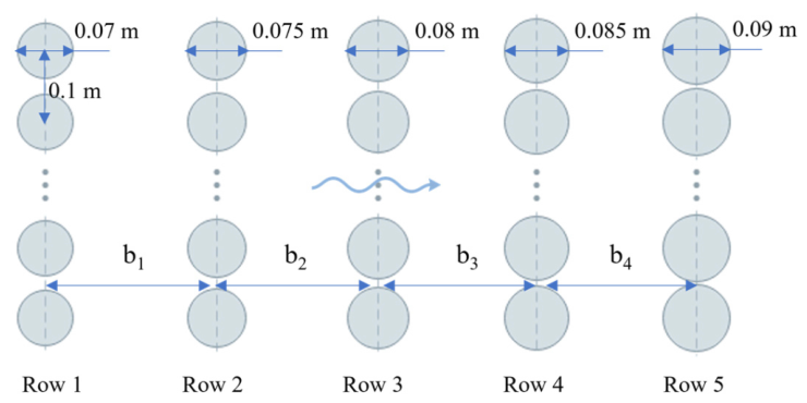
The present work investigates a gradient-porosity distributed multi-row pile breakwater (GPDMPB). It consists of five pile rows with porosities of P₁ = 0.30, P₂ = 0.25, P₃ = 0.20, P₄ = 0.15, and P₅ = 0.10 along the wave-propagation direction. The upstream rows therefore have wider gaps than the downstream rows (see Figure 1). This geometry is intended to distribute wave–structure interactions across successive rows. Whether it improves the balance between reflection and transmission is assessed through the comparisons presented below.

Figure 1. Conceptual illustration of GPDMPB with stepwise porosity gradient.

In this study, the term “phononic-crystal-inspired” refers specifically to the design analogy of varying structural properties along the wave-propagation direction. The proposed breakwater is a finite array with a stepwise porosity gradient, and its performance is evaluated through reflection and transmission coefficients, an energy dissipation coefficient, and simulated flow fields. Dispersion relations, resonance characteristics, and bandgaps are outside the scope of the present analysis. Accordingly, the observed attenuation is discussed in terms of the simulated hydrodynamic interactions around successive pile rows.

The present study investigates the hydrodynamic response of a gradient-porosity multi-row pile breakwater (GPDMPB) under regular-wave conditions. A three-dimensional numerical model based on OpenFOAM and OlaFlow is assessed against available experimental measurements and then used to compare graded and uniform porosity arrangements and examine the effects of pile-row spacing and incident-wave conditions. Reflection, transmission, energy dissipation, and flow-field characteristics are analyzed to characterize wave–structure interactions across the pile array.

2. Numerical Formulation and Model

This study employs OpenFOAM (version 2112) for CFD simulations, combined with the OlaFlow toolbox developed by Higuera [16] to simulate wave generation, propagation and interaction with structures.

2.1. Governing Equations and Free-Surface Modeling

Wave motion around the pile array is described by the incompressible Reynolds-averaged Navier–Stokes equations. Conservation of mass and momentum is expressed as follows:

$${\displaystyle \frac{\partial u_i}{\partial x_i}}=0$$

(1)

$${\displaystyle \frac{\partial \rho u_i}{\partial t}}+{\displaystyle \frac{\partial \rho u_j{u}_i}{\partial x_j}}-{\displaystyle \frac{\partial }{\partial x_j}}\left[{\mu }_{eff}{\displaystyle \frac{\partial u_i}{\partial x_j}}\right]=-{\displaystyle \frac{\partial p^{*}}{\partial x_i}}+F_{b,i}+f_{\sigma ,i}$$

(2)

where t denotes time and u_i denotes the Cartesian components of the fluid velocity in the i-direction (i = x, y, z). Here ρ, μ_eff and p* denote fluid density, effective dynamic viscosity, and pressure relative to the hydrostatic component, respectively. F_bi and F_σi represent the body-force and surface-tension contributions.

Interface evolution is resolved with the volume-of-fluid (VOF) method [17]. The phase indicator α takes a value of zero in the air phase and unity in water, with intermediate values identifying interface cells.

$${\displaystyle \frac{\partial \alpha }{\partial t}}+{\displaystyle \frac{\partial (u_i\alpha )}{\partial x_i}}+{\displaystyle \frac{\partial u_{c,i}\alpha (1-\alpha )}{\partial x_i}}=0$$

(3)

In Equation (3), the third term on the left-hand side represents the artificial compression term, primarily used to limit numerical diffusion. Here, $u_{c,i} = \min \left[c_{\alpha }\left|u_i\right|,max\left(\left|u_i\right|\right)\right]$ represents the relative compression velocity [18]. In Equation (2), density ρ and the effective dynamic viscosity μ_eff are calculated as

$$\rho =\alpha {\rho }_{water}+(1-\alpha ){\rho }_{air}$$

(4)

$${\mu }_{eff}=\alpha {\mu }_{water}+(1-\alpha ){\mu }_{air}+\rho {\nu }_t$$

(5)

Free-surface elevation at each monitoring location is reconstructed from the vertical distribution of α. The water column is divided into n segments, and the interface level is obtained by discrete summation according to Equation (6).

$$z_{water level}={\displaystyle \sum _{i=0}^{n-1}{\alpha }_i}(z_{i+1}-z_i)$$

(6)

In this study, the governing equations were solved using a finite-volume discretization strategy. The pressure-gradient and diffusive terms were approximated with a central differencing scheme, while the divergence operator was discretized by applying a TVD (Total Variation Diminishing) scheme combined with the van Leer limiter. Time integration was carried out using the implicit backward Euler method. The numerical wave flume was established with the olaDyMFlow solver in the olaFlow toolbox. This solver is based on OpenFOAM’s interDyMFoam and incorporates additional capabilities for wave generation and absorption.

2.2. Turbulence Model

Before selecting the turbulence closure, the characteristic Reynolds number was evaluated to assess the flow regime. It is defined as [19]

$$\mathit{Re}=\frac{\stackrel{-}{U}D}{v}=\frac{\mathit{HLD}}{2\mathit{vdT}}$$

(7)

where $\stackrel{-}{U}$ is the depth-averaged amplitude of the horizontal fluid velocity associated with the incident wave. D is the pile diameter, ν is the kinematic viscosity of water, and H, L, T, and d denote the wave height, wavelength, wave period, and still-water depth, respectively. Using the minimum pile diameter of D = 0.07 m gives Re = 10,284, indicating that turbulent effects cannot be neglected in the present simulations.

Conventional turbulence models may generate unrealistically high turbulence levels near the free surface and consequently cause excessive numerical wave damping. Devolder et al. [20] reported this behavior for steep non-breaking waves and subsequently proposed a buoyancy-related correction to the $k-\omega \mathrm{SST}$ model [21]. This modification suppresses spurious turbulence near the air–water interface while retaining the turbulent response in strongly disturbed flow regions. Accordingly, the buoyancy-modified $k-\omega \mathrm{SST}$ model is adopted for the subsequent simulations. The same turbulence-model formulation was applied consistently across all simulated cases to ensure consistency in the comparative analysis. However, a systematic comparison with alternative turbulence models was not conducted. Therefore, the influence of turbulence-model selection on the predicted results has not been independently quantified. In particular, predictions of local flow structures, including flow separation and vortex formation around the pile array, may be affected by the adopted turbulence model.

3. Numerical Model and Validation

3.1. Gradient-Porosity Multi-Row Pile Configuration

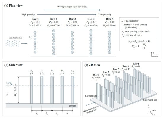
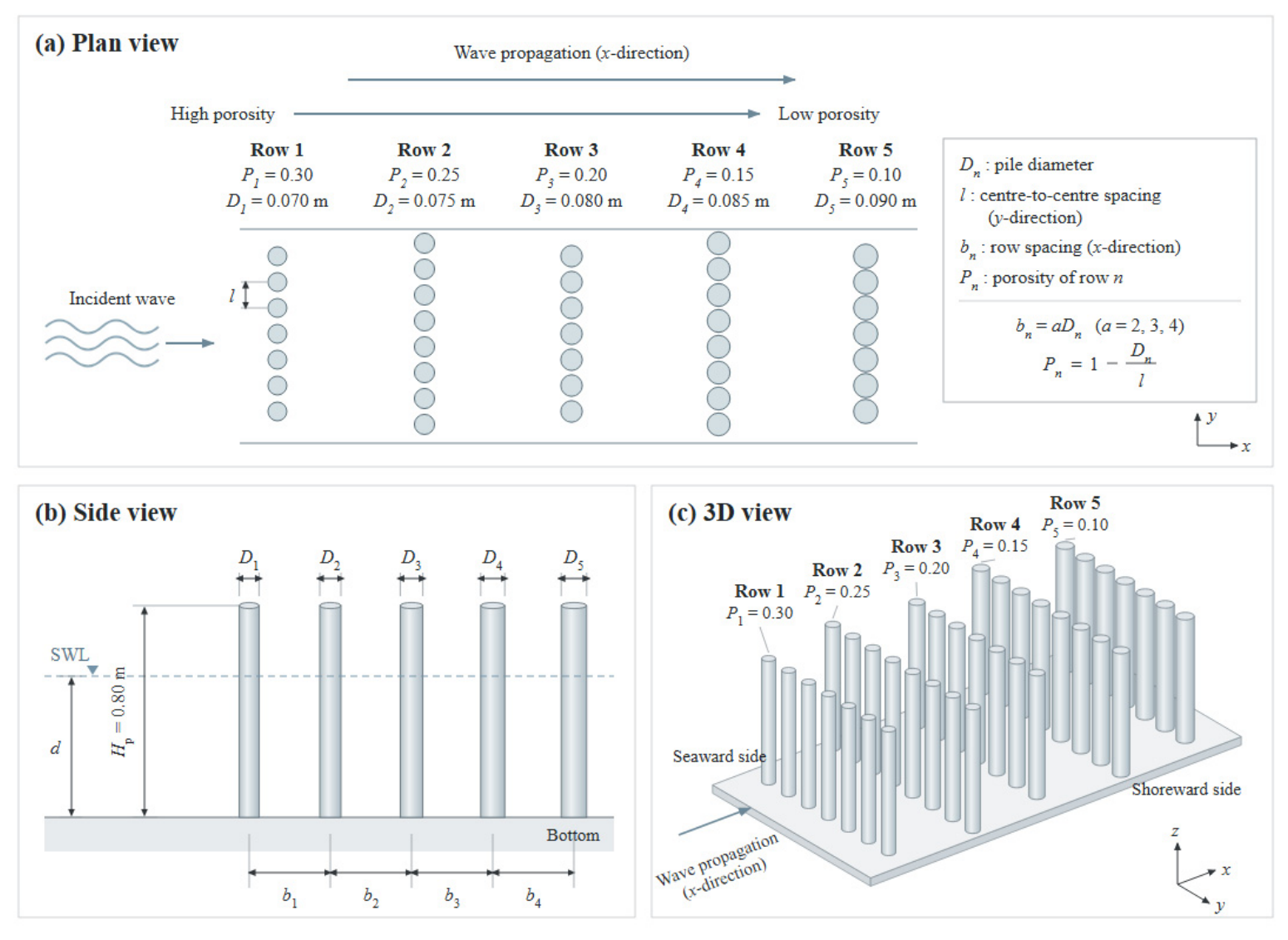
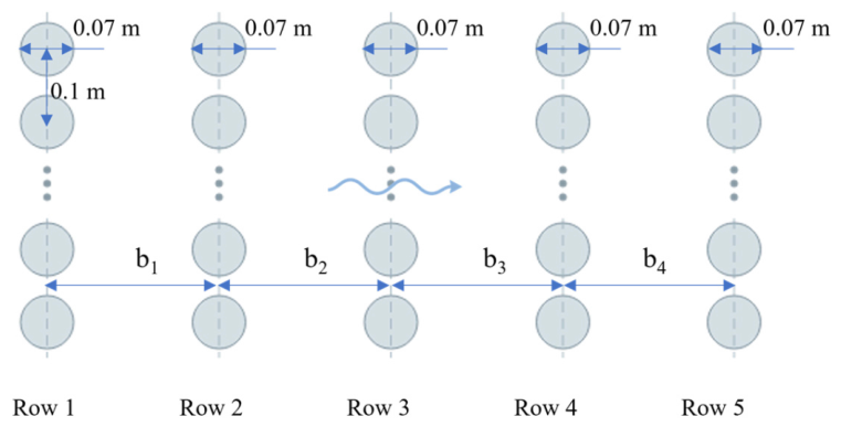
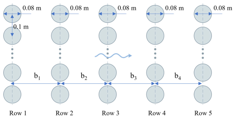
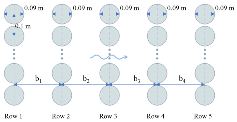
Figure 2 illustrates the configuration of the GPDMPB, which consists of five rows of piles with a uniform pile spacing within each row. The porosity (P) of each row is adjusted by varying the pile diameter. Along the wave propagation direction, the porosity decreases gradually from 0.30 on the seaward side to 0.10 on the shoreward side, with a decrement of 0.05 between adjacent rows. The spacing between adjacent pile rows, b_n, is set to a times the pile diameter of the preceding row, D_n; in the present study, a = 2, 3, and 4. This arrangement forms a functionally graded design aimed at enhancing wave energy dissipation.

Figure 2. Geometric parameters of the GPDMPB: (a) Plan view; (b) Side view; (c) 3D view.

3.2. Numerical Wave Tank and Boundary Conditions

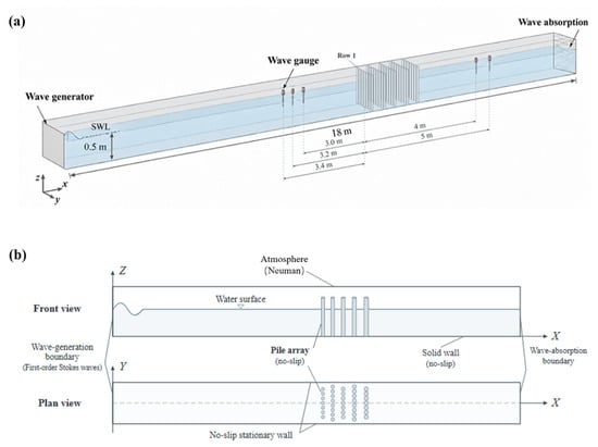
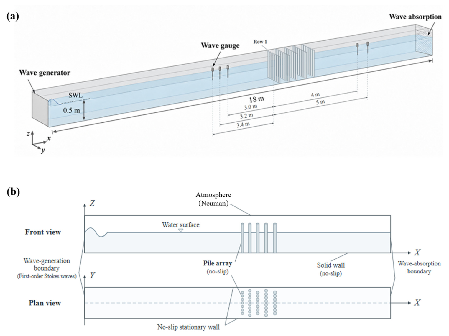
The computational tank used for the GPDMPB simulations measures 18 m × 0.8 m × 0.8 m, with a still-water depth of 0.5 m, as shown in Figure 3. The pile array is located 10 m from the inlet, leaving 8 m between the structure and the downstream end. The x-axis follows the incident-wave direction, y is transverse to the tank, and z points vertically upward.

Figure 3. Schematic of the numerical wave tank and boundary conditions: (a) computational domain and wave-gauge arrangement; (b) boundary conditions and pile-array configuration.

Regular waves are prescribed at the inlet through OlaFlow, while active absorption is imposed at the opposite end to suppress reflected disturbances. No-slip wall conditions are assigned to the bottom and lateral boundaries, and the top boundary is treated as atmospheric. Unless otherwise specified, the same boundary-condition settings are employed in all subsequent simulations. Three upstream gauges, separated by 0.2 m and positioned approximately 3 m ahead of the GPDMPB, provide the surface-elevation records required for incident/reflected-wave separation. Transmission is evaluated from gauges placed behind the structure.

3.3. Mesh Convergence

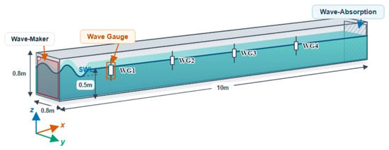
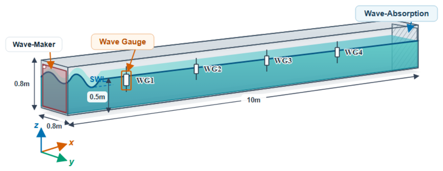
A systematic mesh-dependence analysis was performed to assess the sensitivity of the numerical solution to spatial discretization. For this purpose, a 10 m × 0.8 m × 0.8 m NWT was established for the convergence analysis, as shown in Figure 4. The still-water depth was set to d = 0.5 m and a regular wave with H = 0.10 m and T = 1.0 s was generated. Four wave gauges (WG1–WG4) were arranged along the wave-propagation direction at uniform 2 m intervals to measure the free-surface elevation.

Figure 4. Layout diagram of the NWT for mesh convergence validation.

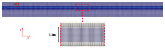
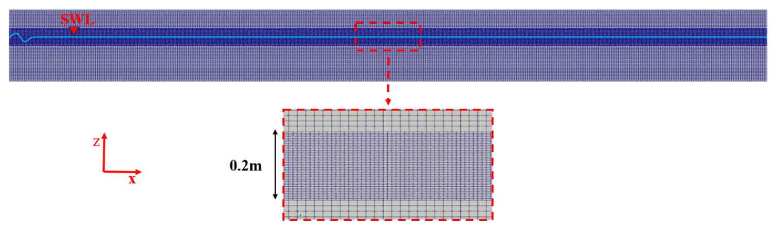
To accurately resolve the air–water interface and minimize numerical dissipation during wave propagation, a local mesh-refinement region was established around the still-water level (SWL). A total refinement height of 2H was adopted, consistent with the mesh-refinement configurations used by Oliveira et al. [22] and Choi et al. [23]. For the present convergence test, this corresponds to a refinement region with a total height of 2H = 0.20 m, as shown in Figure 5.

Figure 5. Mesh refinement.

Within this refined region, the grid spacing in the transverse direction was fixed at Δy = 0.0125 m, while three levels of refinement were considered in the x- and z-directions. The vertical grid sizes were set to H/10, H/20, and H/40 [24] for meshes M1, M2, and M3, respectively. The corresponding streamwise grid sizes were selected such that the grid aspect ratio remained Δx/Δz = 2.5. The resulting mesh configurations are summarized in Table 1.

Table 1. Mesh condition.

Mesh	$\mathbf{\Delta }\mathit{x} \left(\mathbf{m}\right)$	$\mathbf{\Delta }\mathit{y} \left(\mathbf{m}\right)$	$\mathbf{\Delta }\mathit{z} \left(\mathbf{m}\right)$	$\mathbf{\Delta }\mathit{x}$:$\mathbf{\Delta }\mathit{z}$	Number of Cells
M1	0.025	0.0125	0.01	2.5	4.24 × 105
M2	0.0125	0.0125	0.005	2.5	1.49 × 106
M3	0.00625	0.0125	0.0025	2.5	5.54 × 106

The calculation starts with Δt = 0.001 s, after which the time step is adjusted automatically subject to a maximum Courant number of 0.5. Since the Courant number depends on the local flow velocity, cell size, and time step size, this strategy dynamically controls the time step according to the flow conditions and mesh resolution. Each case is advanced for 25 s.

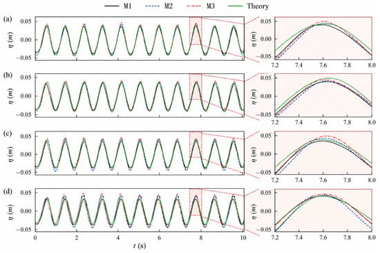
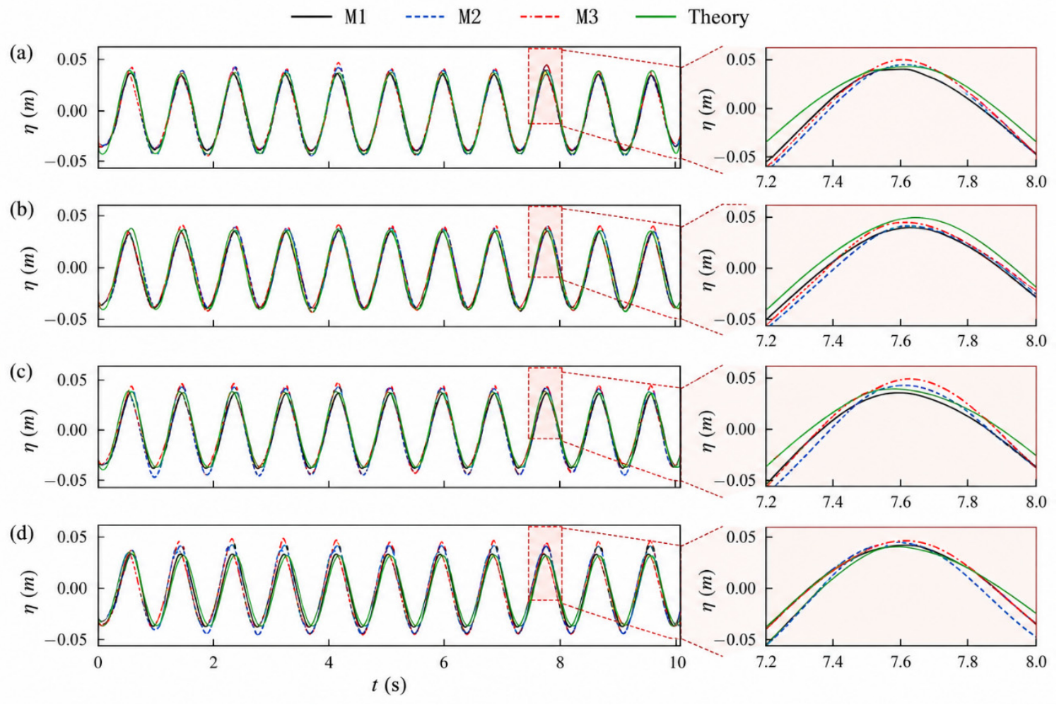
Figure 6 compares the free-surface-elevation histories obtained with the three mesh resolutions at WG1–WG4. All three meshes reproduce the theoretical wave profile reasonably well. The difference between the numerical solutions becomes more apparent as the wave propagates downstream. In particular, M1 exhibits a noticeable phase lag at WG4, whereas the results obtained with M2 and M3 are nearly coincident, indicating that further refinement beyond M2 produces only a limited improvement in the predicted wave propagation.

Figure 6. Comparison of free-surface elevation histories obtained with different mesh resolutions at WG1–WG4: (a) WG1; (b)WG2; (c) WG3; (d) WG4.

A quantitative comparison of the wave-height prediction accuracy and computational cost is summarized in Table 2, further confirming this convergence behavior. The mean wave heights predicted by M1, M2, and M3 are 0.0943, 0.0988, and 0.1005 m, corresponding to errors of 5.7%, 1.2%, and −0.5% from the prescribed wave height of 0.10 m, respectively. Although M3 provides a marginal improvement in accuracy, its computational time increases substantially from 6.50 h for M2 to 51.90 h for M3 on the same 14-core computational platform. This increase is primarily attributed to the larger number of cells and the smaller adaptive time steps required by the finer mesh. The M2 and M3 solutions are almost indistinguishable, whereas M1 develops a visible phase offset at WG4.

Table 2. Error analysis and computational efficiency comparison.

Mesh	$\mathbf{\Delta }\mathit{z} \left(\mathbf{m}\right)$	Wave Height (m)	Computation Time (h)	Error/%
M1	0.01	0.0943	4.72	5.7
M2	0.005	0.0988	6.50	1.2
M3	0.0025	0.1005	51.90	−0.5

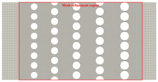
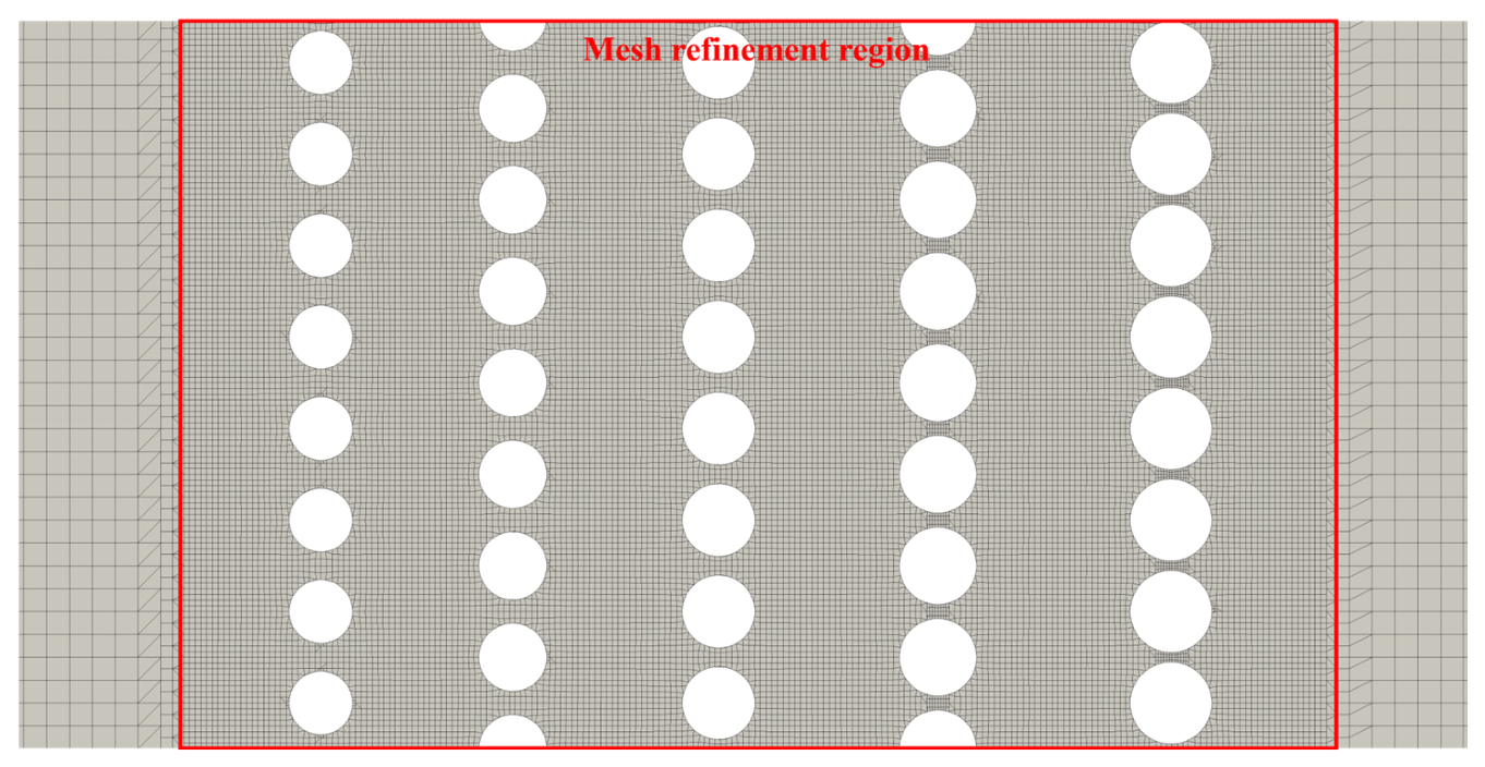
To further investigate mesh sensitivity in the presence of the pile array, Case 1 was selected as a representative configuration, and simulations were performed using three different mesh resolutions. In all simulations involving the pile array, additional local mesh refinement was applied to the region surrounding the structure to better resolve wave–pile interactions, as shown in Figure 7. Specifically, a rectangular refinement region slightly larger than the bounding rectangle of the entire pile array was defined, and the mesh in this region was further refined using the mesh-refinement tools in OpenFOAM. This procedure increased the local mesh resolution around the piles compared with the background mesh. The reflection coefficient $K_r$, transmission coefficient $K_t$, and energy dissipation coefficient $K_e$ were then compared across the three mesh resolutions to assess the sensitivity of the predicted hydrodynamic response to mesh refinement. The results are presented in Table 3.

Figure 7. Local mesh refinement around the pile array.

Table 3. Mesh convergence analysis and wave-gauge pair sensitivity of the GPDMPB.

Mesh	Number of Cells	${\mathit{K}}_{\mathit{r}}$	${\mathit{K}}_{\mathit{t}}$	${\mathit{K}}_{\mathit{e}}$	Computation Time (h)	Relative Range (%)
						${\mathit{K}}_{\mathit{r}}$	${\mathit{K}}_{\mathit{t}}$
M1	1.42 × 106	0.259	0.321	0.911	14	12.4	8.2
M2	3.27 × 106	0.271	0.337	0.902	24	13.4	8.0
M3	5.87 × 106	0.274	0.329	0.904	134	7.1	9.0

The hydrodynamic response was evaluated in terms of the reflection coefficient $K_r$, transmission coefficient $K_t$, and energy dissipation coefficient $K_e$. The reflection and transmission coefficients were defined as follows

$$K_r={\displaystyle \frac{H_r}{H_i}}$$

(8)

$$K_t={\displaystyle \frac{H_t}{H_i}}$$

(9)

where $H_r$, $H_i$, and $H_t$ denote the reflected, incident, and transmitted wave heights, respectively.

Incident and reflected components were obtained using the two-point decomposition procedure of Goda and Suzuki [25]. The three possible gauge pairs were used independently to estimate $K_r$, and the resulting values were averaged to reduce the sensitivity to gauge selection. According to Goda’s study, the normalized gauge spacing, Δx/L, should preferably fall within the range of 0.05–0.45. Gauge spacings equal to integer multiples of half the wavelength should be avoided, as they can lead to singularities in the wave-separation equations and unreliable separation results. For all cases considered in the present study, the normalized spacing of the gauge pairs fell within the recommended range. The transmitted wave height was obtained from the wave gauges located downstream of the structure.

The energy dissipation coefficient is calculated as [26,27]

$$K_e=\sqrt{1-K_r^2-K_t^2}$$

(10)

It should be noted that $K_e$ is an estimate of the overall wave-energy loss inferred from the reflected and transmitted wave components, rather than an independent measurement of local viscous or turbulent energy dissipation. These three coefficients are subsequently used to characterize the redistribution of incident-wave energy among reflection, transmission, and dissipation for the different structural configurations and wave conditions.

To quantify the spread among the wave coefficients calculated using different pairs of wave gauges, the relative range was employed, defined as

$$R_c={\displaystyle \frac{K_{c,\max }-K_{c,\min }}{{\overline{K}}_c}}\times 100\%$$

(11)

where $K_{c,max}$, $K_{c,min}$, and $\overline{K_C}$ denote the maximum, minimum, and mean values of the wave coefficient obtained from the different gauge-pair combinations, respectively.

The relative range was used to quantify the relative variation among the estimates and assess the sensitivity of the calculated wave coefficients to gauge selection.

The simulation results are summarized in Table 3.

Table 3 presents the mesh-convergence results for the GPDMPB configuration, including the hydrodynamic coefficients, computational time, and sensitivity to wave-gauge pair selection. As the mesh is refined from M1 to M3, the reflection, transmission, and energy dissipation coefficients exhibit relatively small variations. In particular, the relative differences between M2 and M3 are 1.09%, 2.43%, and 0.22% for $K_r$, $K_t$, and $K_e$, respectively, indicating that the calculated hydrodynamic coefficients tend to stabilize with mesh refinement. Meanwhile, the relative ranges obtained from different wave-gauge pair combinations are 7.1–13.4% for $K_r$ and 8.0–9.0% for $K_t$, suggesting a moderate sensitivity to gauge-pair selection. Although further mesh refinement from M2 to M3 results in only limited changes in the hydrodynamic coefficients, the computational time increases substantially from 24 h to 134 h. Therefore, considering the balance between numerical accuracy and computational efficiency, M2 is adopted for the subsequent simulations.

3.4. Model Validation

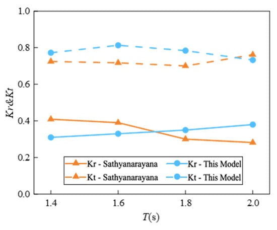
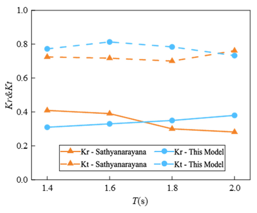
The numerical framework was benchmarked against the rectangular pile-head-breakwater (RPHB) experiments of Sathyanarayana et al. [28]. The validation conditions comprise a water depth of 0.40 m, an incident wave height of 0.10 m, and four wave periods ranging from 1.4 to 2.0 s.

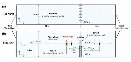
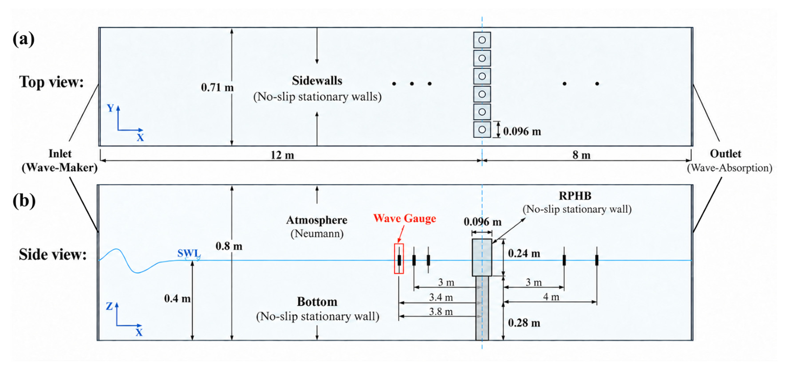
The experimental RPHB geometry was reproduced in an NWT with dimensions of 20 m × 0.71 m × 0.80 m. The enlarged head is 0.096 m wide and 0.24 m high, supported by a pile body with a height of 0.28 m. A 12 m upstream section was retained before the structure, exceeding three times the maximum wavelength of 3.69 m. Three wave gauges were positioned approximately 3 m upstream of the structure, with a spacing of 0.4 m between adjacent gauges, while additional wave gauges downstream were used for transmitted-wave measurements. The layout of the validation NWT and the arrangement of the wave gauges are illustrated in Figure 8. The mesh resolution followed the M2 configuration established in Section 3.3, with Δx = 0.0125 m, Δy = 0.0125 m, and Δz = 0.005 m in the refined free-surface region. The boundary conditions and numerical schemes were kept consistent with those described previously.

Figure 8. Layout of the validation numerical wave tank and arrangement of wave gauges around the RPHB: (a) Top view; (b) side view.

The numerical model was evaluated in terms of the wave reflection coefficient $K_r$ and transmission coefficient $K_t$.

Figure 9 compares the predicted reflection and transmission coefficients with the experimental measurements over the considered wave-period range. The numerical results generally reproduce the experimental trends of both coefficients, although the agreement is better for the transmission coefficient than for the reflection coefficient.

Figure 9. Comparison of the numerically predicted and experimentally measured reflection and transmission coefficients for the RPHB.

To further quantify the agreement between the numerical and experimental results, the normalized root mean square error (NRMSE), normalized by the mean experimental value, was calculated for $K_r$ and $K_t$. The resulting NRMSE values were 23.15% and 9.56%, respectively, indicating better agreement for the transmission coefficient than for the reflection coefficient.

Furthermore, to evaluate the sensitivity of the calculated wave coefficients to wave-gauge selection, the relative range (RR) was determined using the results obtained from different wave-gauge pair combinations. As shown in Table 4, the RR values for $K_r$ were 6.2%, 6.5%, 8.6%, and 3.6% at wave periods of 1.4, 1.6, 1.8, and 2.0 s, respectively, while the corresponding values for $K_t$ were 6.1%, 1.0%, 8.8%, and 4.0%. All RR values were below 10%, indicating relatively limited variation among the estimates obtained from different gauge-pair combinations. These results provide additional support for the consistency of the estimated wave coefficients with respect to gauge selection.

Table 4. Quantitative evaluation of reflection and transmission coefficients.

Wave Coefficient	Relative Range (%)					NRMSE (%)
$K_r$	T (s)	1.4	1.6	1.8	2.0	23.15
	RR (%)	6.2	6.5	8.6	3.6
$K_t$	T (s)	1.4	1.6	1.8	2.0	9.56
	RR (%)	6.1	1.0	8.8	4.0

3.5. Simulation Conditions and Cases

Table 5 lists the incident-wave conditions adopted in the parametric calculations. Four regular-wave periods from T = 0.8 to 1.4 s are considered, corresponding to wavelengths of 0.995–2.571 m. Unless otherwise specified, the incident wave height was fixed at H = 0.10 m. Two additional wave heights, H = 0.08 and 0.12 m, were introduced to investigate the influence of wave steepness. The resulting wave steepness H/L ranges from 0.031 to 0.121 over the investigated conditions.

Table 5. Wave Conditions.

Wave Conditions	T (s)	L (m)	H (m)	H/L
W1	0.8	0.995	0.080/0.100/0.120	0.080/0.101/0.121
W2	1.0	1.513		0.053/0.066/0.079
W3	1.2	2.058		0.039/0.049/0.058
W4	1.4	2.571		0.031/0.039/0.047

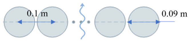
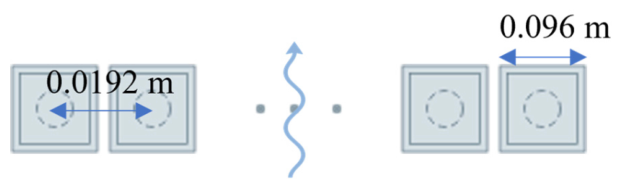
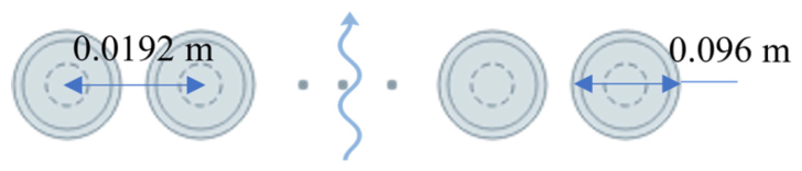
A total of eleven numerical cases were designed to systematically examine the influence of structural configuration and incident-wave conditions on the hydrodynamic response of the GPDMPB, as summarized in Table 6. Case 1 represents the reference GPDMPB configuration, consisting of five staggered pile rows with a stepwise porosity distribution of P₁ = 0.30, P₂ = 0.25, P₃ = 0.20, P₄ = 0.15, and P₅ = 0.10 along the wave-propagation direction. Cases 2–4 were introduced as reference configurations for comparison with conventional permeable breakwaters. These include a single-row pile breakwater, the square enlarged pile-head breakwater proposed by Sathyanarayana et al. [28] and the enlarged pile-head breakwater reported by Suvarna et al. [29]. For a consistent comparison, the elevations of the comparative structures were adjusted such that the incident waves acted approximately at the mid-height of their principal wave-dissipating regions.

Table 6. Structures used for simulation.

Simulation Case	Structure	Geometric Parameters
Case 1 Gradient distribution	P1 = 0.3, P2 = 0.25, P3 = 0.2, P4 = 0.15, P5 = 0.1, bn = 3Dn	Pile count: 40 Footprint: 0.808 m2 Total blockage: 1.60 m2
Case 2	P = 0.10	Pile count: 8 Footprint: 0.72 m2 Total blockage: 0.36 m2
Case 3	P = 0.17	Pile count: 6 Footprint: 0.068 m2 Total blockage: 0.16 m2
Case 4	P = 0.17	Pile count: 6 Footprint: 0.068 m2 Total blockage: 0.15 m2
Case 5 Uniform distribution	P1 = P2 = P3 = P4 = P5 = 0.3, bn = 3Dn	Pile count: 40 Footprint: 0.728 m2 Total blockage: 1.40 m2
Case 6 Uniform distribution	P1 = P2 = P3 = P4 = P5 = 0.2, bn = 3Dn	Pile count: 40 Footprint: 0.832 m2 Total blockage: 1.60 m2
Case 7 Uniform distribution	P1 = P2 = P3 = P4 = P5 = 0.1, bn = 3Dn	Pile count: 40 Footprint: 0.936 m2 Total blockage: 1.80 m2
Cases 8–9	P1 = 0.3, P2 = 0.25, P3 = 0.2, P4 = 0.15, P5 = 0.1, bn = aDn In these cases, a = 2 for Case 8 and a = 4 for Case 9	Pile count: 40 Footprint: Case 8: 0.560 m2 Case 9: 1.056 m2 Total blockage: 1.60 m2
Cases 10–11	Same structural configuration as Case 1, with wave heights of 0.08 m and 0.12 m.	Same as Case 1.

Cases 5–7 correspond to five-row pile breakwaters with uniform porosity distributions of P = 0.30, 0.20 and 0.10, respectively. These cases were used to distinguish the effect of the graded porosity arrangement from that of uniformly distributed pile arrays. Cases 8 and 9 retain the same porosity gradient as Case 1 but employ different row-spacing parameters to investigate the sensitivity of wave attenuation to the spacing between successive pile rows. Finally, Cases 10 and 11 adopt the same structural configuration as Case 1 with incident wave heights of H = 0.08 and 0.12 m, respectively, to examine the influence of wave steepness. For all other cases, the incident wave height was maintained at H = 0.10 m.

The hydrodynamic response of the different configurations is evaluated using the reflection coefficient $K_r$, transmission coefficient $K_t$ and energy dissipation coefficient $K_e$.

4. Results and Discussion

This section examines the hydrodynamic response of the GPDMPB through comparisons with conventional permeable breakwaters and uniform-porosity pile arrays, followed by analyses of pile-row spacing and wave steepness. Particular attention is given to the redistribution of incident-wave energy through successive wave–structure interactions within the spatially graded pile array.

4.1. Comparison with Conventional Permeable Breakwaters

This subsection presents a comparative analysis of the wave attenuation performance between the GPDMPB and several conventional permeable breakwaters.

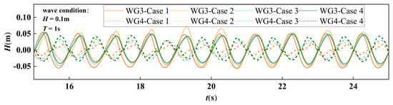
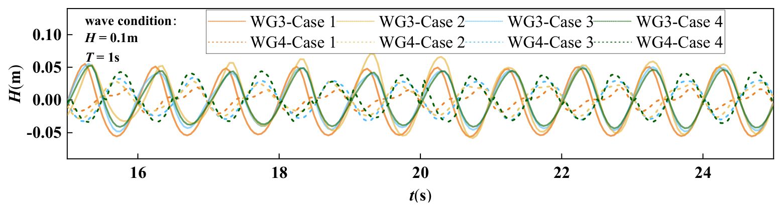
Figure 10 shows the time histories of surface elevations recorded at WG3, located in front of the structures, and WG4, located behind the structures, under identical incident wave conditions. Compared with the conventional permeable breakwaters, the GPDMPB produces a noticeably lower wave amplitude at WG4, indicating its stronger ability to suppress transmitted waves.

Figure 10. The time histories of surface elevations for GPDMPB and conventional permeable breakwaters at WG3 and WG4 (H = 0.1 m, T = 1 s).

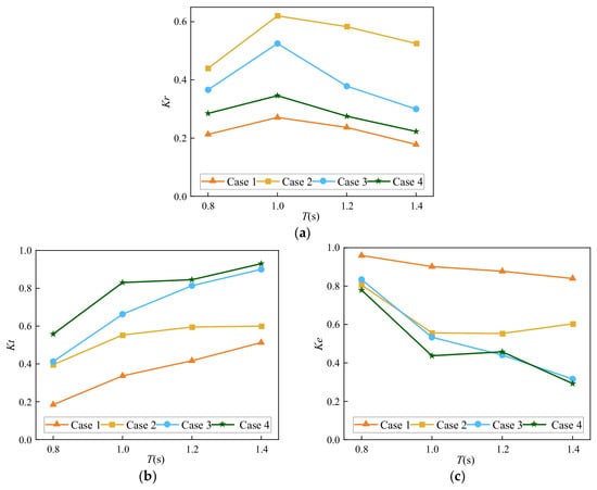
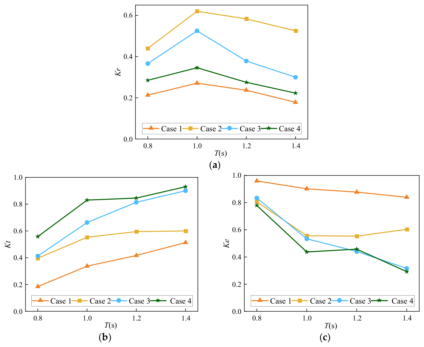
Figure 11 compares the reflection, transmission, and dissipation characteristics of the GPDMPB with those of the three conventional permeable breakwaters. Across the investigated wave-period range, Case 1 generally maintains lower $K_r$ and $K_t$, together with a higher $K_e$, indicating better overall wave attenuation performance than the three comparison configurations under the examined conditions.

Figure 11. Wave reflection, transmission, and dissipation coefficients of GPDMPB and conventional permeable breakwaters against: T (a) Reflection coefficients; (b) Transmission coefficients; (c) Energy dissipation coefficients.

Table 7 provides a quantitative comparison of the hydrodynamic coefficients of Cases 1–4 normalized by those of Case 1 at the same wave period. The normalized results show that the conventional permeable breakwaters produce reflection coefficients 1.16–2.94 times those of the GPDMPB and transmission coefficients 1.16–3.01 times those of the GPDMPB. Meanwhile, their energy dissipation coefficients are only 0.35–0.87 times those of the GPDMPB. These results indicate that the GPDMPB achieves favorable wave attenuation performance compared with the conventional permeable breakwater configurations considered, as reflected by its lower reflection and transmission coefficients and higher energy dissipation coefficient under the investigated wave conditions.

Table 7. Hydrodynamic coefficients normalized by Case 1 under different wave periods.

T (s)	Coefficient	Case 1	Case 2	Case 3	Case 4
0.8	Kr/Kr,ref	1.00	2.06	1.72	1.34
	Kt/Kt,ref	1.00	2.14	2.23	3.01
	Ke/Ke,ref	1.00	0.84	0.87	0.81
1	Kr/Kr,ref	1.00	2.29	1.94	1.28
	Kt/Kt,ref	1.00	1.64	1.96	2.46
	Ke/Ke,ref	1.00	0.62	0.59	0.49
1.2	Kr/Kr,ref	1.00	2.46	1.60	1.16
	Kt/Kt,ref	1.00	1.43	1.95	2.04
	Ke/Ke,ref	1.00	0.63	0.50	0.52
1.4	Kr/Kr,ref	1.00	2.94	1.68	1.25
	Kt/Kt,ref	1.00	1.16	1.75	1.81
	Ke/Ke,ref	1.00	0.71	0.38	0.35

4.2. Effect of Porosity Distribution

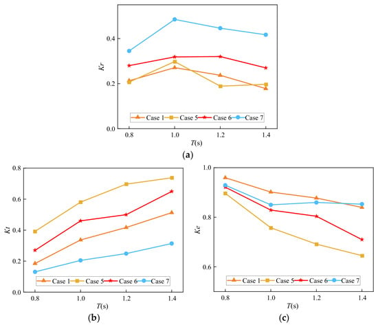
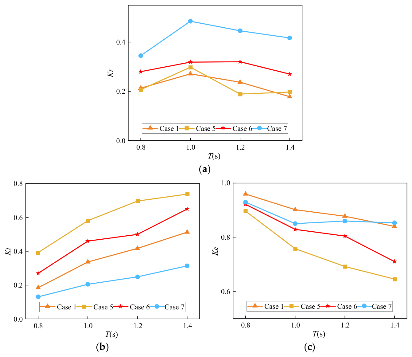
This subsection aims to compare the uniform and gradient-porosity distribution schemes, examining their effects on the wave dissipation performance of breakwaters. The detailed simulation results are shown in Figure 12.

Figure 12. Wave reflection, transmission, and dissipation coefficients for different porosity distribution schemes against T: (a) Reflection coefficients; (b) Transmission coefficients; (c) Energy dissipation coefficients.

Figure 12 presents the variations in the reflection, transmission, and energy dissipation coefficients of different porosity-distribution configurations with wave period. As shown in Figure 12a, the reflection coefficients generally increase from T = 0.8 s to T = 1.0 s and subsequently decrease or remain relatively stable. In contrast, the transmission coefficients increase with increasing wave period for all configurations, while the energy dissipation coefficients generally exhibit a decreasing trend, as shown in Figure 12b,c. Compared with the GPDMPB (Case 1), the uniform-porosity configuration of 0.30 (Case 5) exhibits lower reflection but higher transmission, whereas the uniform-porosity configuration of 0.10 (Case 7) exhibits higher reflection but lower transmission. Notably, the reflection coefficient of the GPDMPB is comparable to that of the uniform-porosity configuration of 0.30 and substantially lower than that of the uniform-porosity configuration of 0.10. These comparisons illustrate the trade-off between reflection and transmission associated with the graded porosity configuration. More importantly, Case 1 and Case 6 have the same total blockage but exhibit distinct hydrodynamic responses. Although Cases 1 and 6 have the same total blockage, their hydrodynamic responses differ. Compared with Case 6, Case 1 exhibits lower transmission and generally lower or comparable reflection, together with a higher energy-dissipation coefficient. This comparison indicates that the spatial arrangement of porosity is associated with differences in hydrodynamic response even when the total blockage is matched.

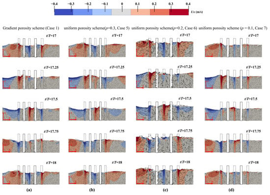
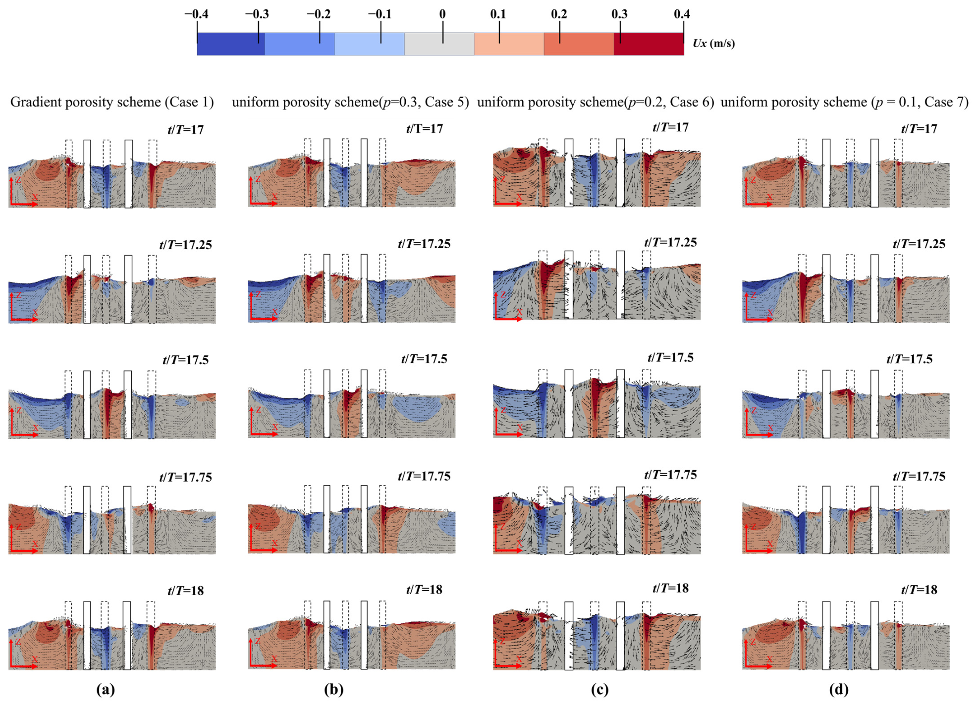
To further investigate the influence of porosity distribution on wave attenuation, Figure 13 compares the instantaneous flow fields of four porosity configurations over a complete wave cycle. At t/T = 17, the incident wave crest reaches the first row of piles and begins to interact with the structure. As the wave propagates through the pile array, local flow acceleration occurs within the pile gaps, accompanied by flow separation and recirculation around the piles. At t/T = 17.25 and 17.5, differences in the flow patterns among the configurations become more apparent, particularly in front of the first pile row and within the structure. Compared with Cases 6 and 7, Cases 1 and 5 have a higher porosity in the first pile row, allowing the incident wave to pass through relatively wider gaps. Consequently, weaker backflow develops in front of the structure, and lower local flow velocities are observed through the gaps into the first chamber. In contrast, the lower porosity of the first pile row in Cases 6 and 7 produces stronger flow obstruction and local contraction effects, resulting in more pronounced upstream backflow and higher velocities through the narrower gaps.

Figure 13. Flow field on vertical cross section of y = 0.4 m at different times in a period (T = 1 s, H = 0.1 m): (a) Graded porosity scheme; (b) uniform scheme (P = 0.3); (c) uniform scheme (P = 0.20); (d) uniform scheme (P = 0.10).

However, considering the propagation of the wave crest through the entire structure, Case 1 exhibits stronger wave attenuation than Case 5. Although both configurations have the same porosity in the first pile row, the porosity of Case 1 progressively decreases along the wave-propagation direction, whereas Case 5 maintains a uniform porosity of 0.30. Consequently, the wave encounters increasing flow resistance as it propagates through successive pile rows in Case 1, leading to more pronounced flow disturbance and attenuation within the structure. In contrast, the relatively high porosity maintained throughout Case 5 allows the wave to propagate more readily through the pile array, resulting in greater wave transmission.

Notably, although Case 1 and Case 6 have the same total blockage, the GPDMPB (Case 1) exhibits weaker backflow in front of the structure and reduced wave transmission behind the structure compared with Case 6. The flow fields show weaker upstream backflow and lower downstream wave amplitudes for Case 1 than for Case 6. Together with the hydrodynamic coefficients in Figure 12, these observations indicate that the porosity arrangement is associated with differences in local flow patterns and wave transmission under the matched-blockage comparison. Together with the hydrodynamic coefficients presented in Figure 12, these observations suggest that the graded porosity arrangement can improve the balance between wave reflection and transmission by distributing wave–structure interactions across successive pile rows under the investigated conditions.

4.3. Effect of Pile-Row Spacing

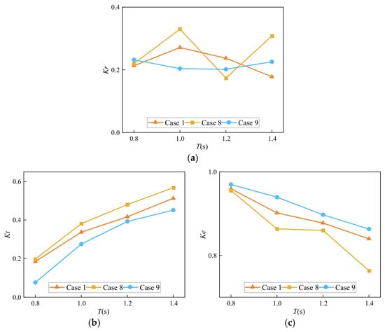
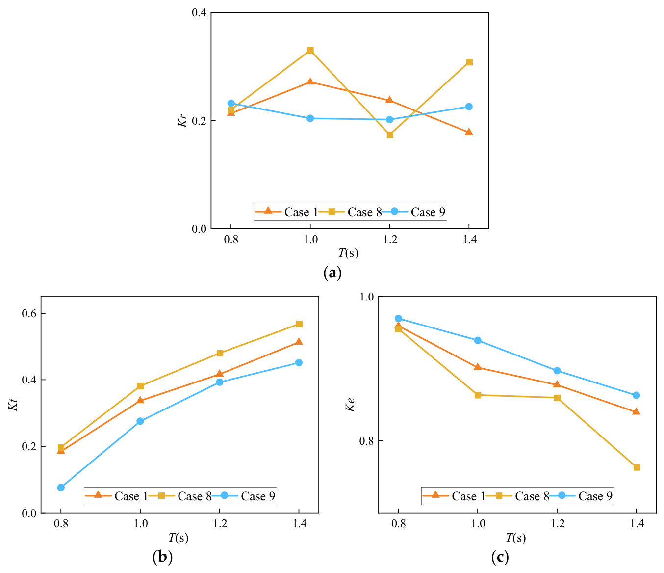
To investigate the influence of pile-row spacing on the hydrodynamic response of the GPDMPB, Cases 8, 1, and 9 were compared. These three cases employ the same graded porosity distribution, while the row-spacing parameter a is set to 2, 3, and 4, respectively. Therefore, the comparison isolates the effect of the spacing between successive pile rows on wave reflection, transmission, and energy dissipation. The corresponding results are presented in Figure 14.

Figure 14. Wave coefficients of the GPDMPB with different pile-row spacings: (a) reflection coefficients; (b) transmission coefficients; (c) energy dissipation coefficients.

As shown in Figure 14a, the reflection coefficient exhibits a non-monotonic dependence on pile-row spacing, and the relative performance of the three configurations varies with the incident wave period. At T = 0.8 s, Cases 1 and 8 exhibit relatively low reflection coefficients. At T = 1.0 s, Case 9 produces the lowest $K_r$, whereas Case 8 gives the lowest value at T = 1.2 s. When the wave period increases to T = 1.4 s, Case 1 exhibits the lowest reflection coefficient. These results indicate that the effect of row spacing on wave reflection depends on the incident wave condition, and no single spacing consistently minimizes wave reflection over the entire range of wave periods investigated.

Figure 14b shows that the transmission coefficient $K_t$ generally increases with wave period for Cases 8, 1, and 9. The differences in $K_t$ among the three configurations remain relatively small over the investigated wave-period range, although they are more apparent at shorter wave periods. Compared with reflection, transmission is less sensitive to pile-row spacing under the conditions considered.

The corresponding energy dissipation coefficients are shown in Figure 14c. The three configurations maintain relatively high $K_e$ values, although variations in row spacing lead to measurable differences in energy dissipation under different wave periods. These variations reflect the combined changes in wave reflection and transmission induced by the spatial separation between successive pile rows. Increasing or decreasing the row spacing changes the distance over which the wave interacts with successive rows and consequently modifies the cumulative hydrodynamic response of the multi-row structure. Nevertheless, the results do not indicate a universally preferable spacing for all incident-wave conditions. Instead, the influence of row spacing is wave-period dependent and should be considered together with the corresponding reflection, transmission, and dissipation characteristics.

Overall, pile-row spacing is an important geometric parameter influencing the hydrodynamic response of the GPDMPB, particularly its wave-reflection characteristics. Within the investigated range, variations in spacing have a more pronounced effect on $K_r$ than on $K_t$ while $K_e$ remains relatively high across all three configurations. However, increasing pile-row spacing also increases the longitudinal width of the breakwater. Therefore, an appropriate spacing should be selected by considering both hydrodynamic performance and structural footprint. These results characterize the spacing-dependent hydrodynamic response of the GPDMPB configurations under the investigated wave conditions.

4.4. Effect of Wave Steepness

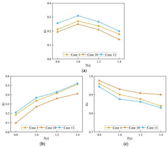
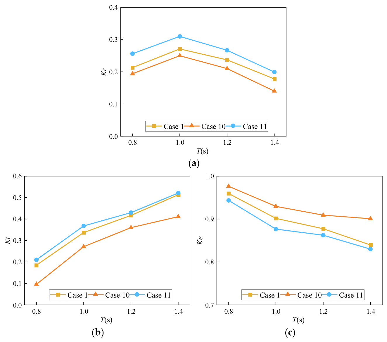
The influence of wave steepness on the hydrodynamic response of the GPDMPB was investigated using Cases 10, 1, and 11, corresponding to incident wave heights of H = 0.08, 0.10, and 0.12 m, respectively. For a given wave period, the wavelength remains unchanged under the prescribed wave conditions; therefore, varying the incident wave height directly changes the wave steepness H/L. The resulting reflection, transmission, and energy dissipation coefficients are presented in Figure 15.

Figure 15. Wave coefficients of the GPDMPB under different wave-steepness conditions: (a) Reflection coefficients; (b) Transmission coefficients; (c) Energy dissipation coefficients.

As shown in Figure 15a–c, wave steepness has a systematic influence on the hydrodynamic response of the GPDMPB. For the same wave period, both the reflection coefficient $K_r$ and transmission coefficient $K_t$ generally increase with increasing incident wave height, whereas the corresponding energy dissipation coefficient $K_e$ decreases. This trend indicates that, under higher-wave-steepness conditions, a greater portion of the incident-wave response is manifested through reflection on the seaward side and transmission toward the downstream region, while the relative contribution represented by $K_e$ is reduced.

The flow fields show more pronounced upstream backflow under the higher-wave-height condition, consistent with the corresponding increase in the reflection coefficient. At the same time, the increase in $K_t$ indicates that a larger transmitted-wave component is able to propagate through the pile gaps and successive chambers of the GPDMPB. Although the graded pile arrangement continues to attenuate the incident wave through repeated interactions with successive pile rows, its relative attenuation effectiveness decreases as the wave steepness increases. Consequently, the distribution among reflection, transmission, and dissipation changes progressively with incident wave height.

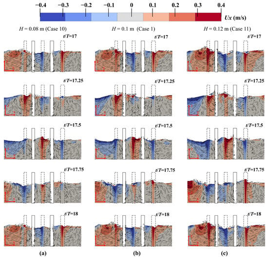
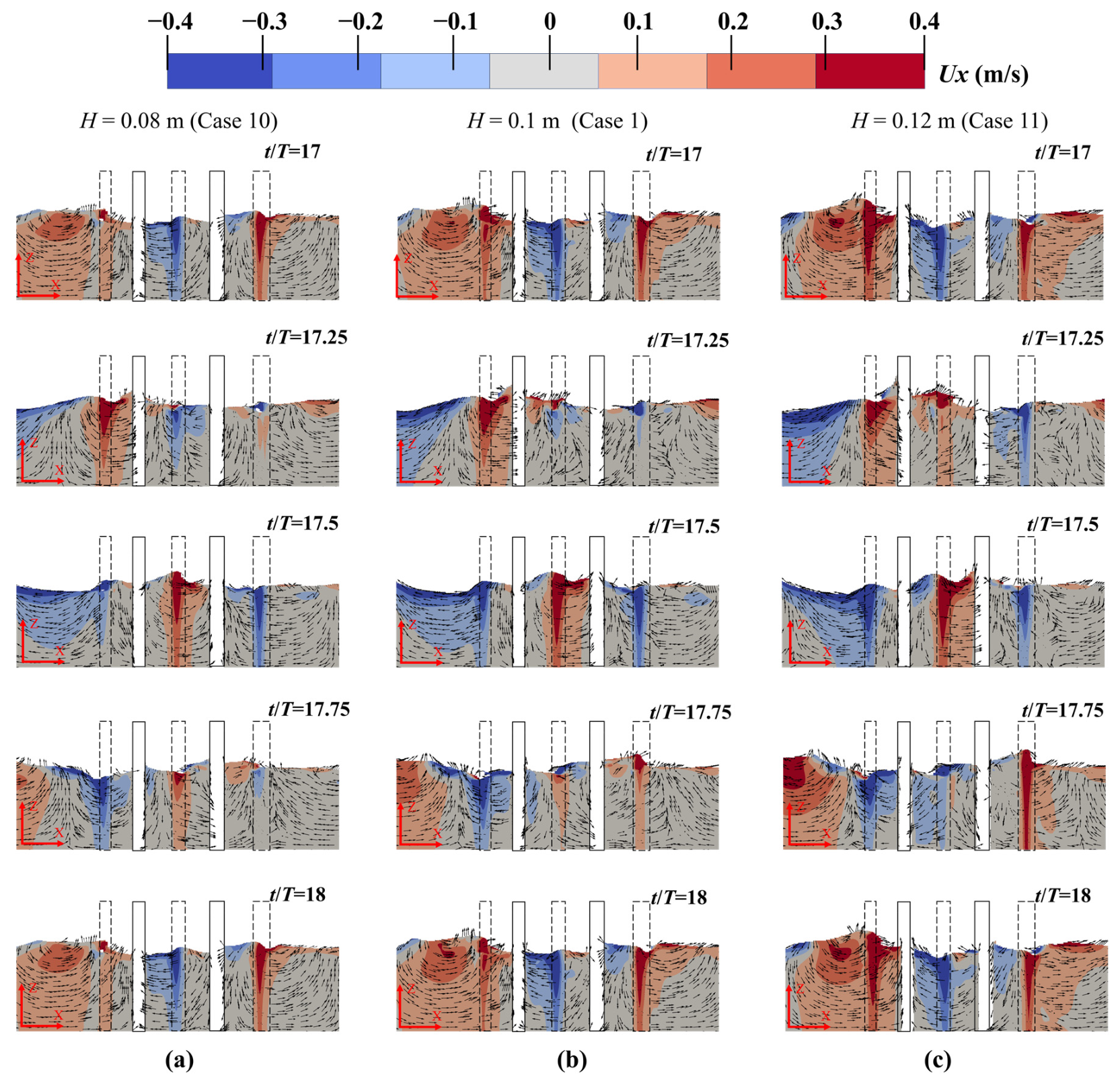
To further examine the corresponding flow characteristics, Figure 16 compares the wave–structure interaction processes over one wave cycle for H = 0.08, 0.10, and 0.12 m at the same wave period. The snapshots illustrate the evolution of the velocity field and recirculation patterns as the wave propagates through the graded pile array.

Figure 16. Flow field on vertical cross section of y = 0.4 m at different times in a period (T = 1 s). (a) H = 0.08 m; (b) H = 0.1 m; (c) H = 0.12 m.

At t/T = 17, when the wave crest approaches the first pile row, clear differences in the local flow field can already be observed among the three wave-height conditions. Case 11 (H = 0.12 m) exhibits a more pronounced high-velocity region on the seaward side of the structure, together with stronger streamline deflection around the first pile row. As the wave propagates further into the structure at t/T = 17.25, a larger recirculation region develops upstream of the first row for Case 11, consistent with the higher reflection coefficient observed under the larger-wave-height condition.

During subsequent propagation through the pile array, the higher-wave-height case also exhibits stronger local flow acceleration through the pile gaps, together with more pronounced flow separation and recirculation around successive pile rows. These flow features are consistent with the changes in the reflection and transmission coefficients observed under the different wave-height conditions. In contrast, Cases 1 and 10 exhibit relatively weaker local velocity gradients and smaller recirculation regions. The comparison therefore suggests that increasing wave steepness intensifies the local hydrodynamic interaction around the piles and modifies the manner in which the incident-wave response is redistributed among reflection, transmission, and dissipation.

Within the investigated range, increasing wave height generally increases the reflection and transmission coefficients while reducing the energy-dissipation coefficient at a given wave period. The flow fields show local acceleration, separation, and recirculation around successive pile rows under all three wave-height conditions, with differences in the extent of these features. These observations are consistent with the changes in the hydrodynamic coefficients as wave steepness increases.

5. Conclusions

A gradient-porosity distributed multi-row pile breakwater (GPDMPB), with porosity decreasing along the wave-propagation direction, was proposed and numerically investigated. Compared with the conventional permeable breakwater configurations examined, the graded configuration exhibited lower reflection and transmission coefficients and a higher energy-dissipation coefficient under the investigated conditions. Comparisons with uniform-porosity arrays P = 0.30 and P = 0.10 revealed a trade-off between reflection and transmission: decreasing porosity reduced transmission but increased reflection. Compared with a uniform-porosity array P = 0.20 having the same total blockage, the graded configuration exhibited lower transmission, generally lower or comparable reflection, and a higher energy-dissipation coefficient. These comparisons indicate that the spatial arrangement of porosity influences the hydrodynamic response of the finite pile array beyond total blockage alone.

Pile-row spacing had a wave-period-dependent influence on the hydrodynamic response. Reflection varied non-monotonically with spacing, whereas transmission was comparatively less sensitive to spacing within the investigated range. These results suggest that pile-row spacing should be considered in conjunction with incident-wave conditions when selecting the structural configuration. Increasing wave steepness generally increased the reflection and transmission coefficients while reducing the energy-dissipation coefficient.

The flow-field results showed local acceleration, flow separation, and recirculation around successive pile rows, consistent with the observed changes in the hydrodynamic coefficients. Overall, the results indicate that a stepwise porosity gradient can help balance reflection and transmission in a multi-row pile breakwater under the investigated regular-wave conditions. Further physical-model experiments and investigations under irregular-wave conditions would help assess the applicability of the proposed configuration to a broader range of wave conditions.

References

- Liu, J.; Guo, H.; Wang, T.-T. A Review of Acoustic Metamaterials and Phononic Crystals. Crystals 2020, 10, 305. [Google Scholar] [CrossRef] [Scilit]
- Zhang, S.; Liu, J.; Zhang, H.; Wang, S. Tunable Low Frequency Band Gap and Waveguide of Phononic Crystal Plates with Different Filling Ratio. Crystals 2021, 11, 828. [Google Scholar] [CrossRef] [Scilit]
- Chuang, K.-C.; Wang, D.-F.; Liu, J.-J.; Liao, C.-Y. Linking Time-Domain Vibration Behaviors to Spatial-Domain Propagating Waves in a Leaf-like Gradient-Index Phononic Crystal Lens. Crystals 2021, 11, 1490. [Google Scholar] [CrossRef] [Scilit]
- Jin, Y.; Djafari-Rouhani, B.; Torrent, D. Gradient index phononic crystals and metamaterials. Nanophotonics 2019, 8, 685–701. [Google Scholar] [CrossRef] [Scilit]
- Zhu, S.; Zhao, X.; Han, L.; Zi, J.; Hu, X.; Chen, H. Controlling water waves with artificial structures. Nat. Rev. Phys. 2024, 6, 231–245. [Google Scholar] [CrossRef] [Scilit]
- Hu, X.; Shen, Y.; Liu, X.; Fu, R.; Zi, J.; Jiang, X.; Feng, S. Band structures and band gaps of liquid surface waves propagating through an infinite array of cylinders. Phys. Rev. E 2003, 68, 037301. [Google Scholar] [CrossRef] [Scilit]
- Li, Y.; Mei, C.C. Multiple resonant scattering of water waves by a two-dimensional array of vertical cylinders: Linear aspects. Phys. Rev. E 2007, 76, 016302. [Google Scholar] [CrossRef] [Scilit]
- Bennetts, L.G.; Peter, M.A.; Craster, R.V. Graded resonator arrays for spatial frequency separation and amplification of water waves. J. Fluid Mech. 2018, 854, R4. [Google Scholar] [CrossRef] [Scilit]
- Archer, A.J.; Wolgamot, H.A.; Orszaghova, J.; Bennetts, L.G.; Peter, M.A.; Craster, R.V. Experimental realization of broadband control of water-wave-energy amplification in chirped arrays. Phys. Rev. Fluids 2020, 5, 062801. [Google Scholar] [CrossRef] [Scilit]
- Li, Z.; Wang, Z.; Liang, B.; Zhu, P. Laboratory investigation of the hydrodynamic performance of a pile-supported breakwater with a permeable curved superstructure and rock-fill layer. Ocean Eng. 2025, 337, 121945. [Google Scholar] [CrossRef] [Scilit]
- Ramnarayan, S.K.; Sundar, V.; Sannasiraj, S.A. Hydrodynamic performance of concave front pile-supported breakwaters integrated with a louver wave screen. Ocean Eng. 2022, 254, 111394. [Google Scholar] [CrossRef] [Scilit]
- Ramnarayan, S.K.; Sannasiraj, S.A.; Sundar, V. Hydrodynamic characteristics of curved front face pile-supported breakwaters in random waves. Appl. Ocean Res. 2021, 117, 102922. [Google Scholar] [CrossRef] [Scilit]
- Ramnarayan, S.K.; Sannasiraj, S.A.; Sundar, V. Hydrodynamic characteristics of curved and vertical front face pile-supported breakwaters in regular waves. Ocean Eng. 2020, 216, 108105. [Google Scholar] [CrossRef] [Scilit]
- Rageh, O.S.; Koraim, A.S.; Salem, T.N. Hydrodynamic efficiency of partially immersed caissons supported on piles. Ocean Eng. 2009, 36, 1112–1118. [Google Scholar] [CrossRef] [Scilit]
- Vu, M.-T.; Pham, M.-Q.; Vu, Q.-H. Numerical study on hydrodynamic characteristics of new modified pile-supported breakwater. Ocean Eng. 2024, 312, 119141. [Google Scholar] [CrossRef] [Scilit]
- Higuera, P. Enhancing active wave absorption in RANS models. Appl. Ocean Res. 2020, 94, 102000. [Google Scholar] [CrossRef] [Scilit]
- Hirt, C.W.; Nichols, B.D. Volume of fluid (VOF) method for the dynamics of free boundaries. J. Comput. Phys. 1981, 39, 201–225. [Google Scholar] [CrossRef] [Scilit]
- Rusche, H. Computational Fluid Dynamics of Dispersed Two-Phase Flows at High Phase Fractions. Ph.D. Thesis, Imperial College London, London, UK, 2003. [Google Scholar]
- Wang, D.-x.; Dong, S.; Sun, J.-w. Numerical modeling of the interactions between waves and a Jarlan-type caisson breakwater using OpenFOAM. Ocean Eng. 2019, 188, 106230. [Google Scholar] [CrossRef] [Scilit]
- Devolder, B.; Rauwoens, P.; Troch, P. Application of a buoyancy-modified SST turbulence model to simulate wave run-up around a monopile subjected to regular waves using OpenFOAM. Coast. Eng. 2017, 125, 81–94. [Google Scholar] [CrossRef] [Scilit]
- Devolder, B.; Troch, P.; Rauwoens, P. Performance of a buoyancy-modified and SST turbulence model for simulating wave breaking under regular waves using OpenFOAM. Coast. Eng. 2018, 138, 49–65. [Google Scholar] [CrossRef] [Scilit]
- Oliveira, D.; Lopes de Almeida, J.P.P.G.; Santiago, A.; Rigueiro, C. Development of a CFD-Based Numerical Wave Tank of a Novel Multipurpose Wave Energy Converter. Renew. Energy 2022, 199, 226–245. [Google Scholar] [CrossRef] [Scilit]
- Choi, Y.-M.; Bouscasse, B.; Ducrozet, G.; Seng, S.; Ferrant, P.; Kim, E.-S.; Kim, Y.-J. An Efficient Methodology for the Simulation of Nonlinear Irregular Waves in Computational Fluid Dynamics Solvers Based on the High Order Spectral Method with an Application with OpenFOAM. Int. J. Nav. Archit. Ocean Eng. 2023, 15, 100510. [Google Scholar] [CrossRef] [Scilit]
- Qiao, D.; Feng, C.; Yan, J.; Liang, H.; Ning, D.; Li, B. Numerical simulation and experimental analysis of wave interaction with a porous plate. Ocean Eng. 2020, 218, 108106. [Google Scholar] [CrossRef] [Scilit]
- Goda, Y.; Suzuki, Y. Estimation of incident and reflected waves in random wave experiments. Coast. Eng. 1976, 15, 828–845. [Google Scholar] [CrossRef] [Scilit]
- Neelamani, S.; Rajendran, R. Wave interaction with T-type breakwaters. Ocean Eng. 2002, 29, 151–175. [Google Scholar] [CrossRef] [Scilit]
- Madsen, O.S. Wave Transmission through Porous Structures. J. Waterw. Harb. Coast. Eng. Div. 1974, 100, 169–188. [Google Scholar] [CrossRef] [Scilit]
- Sathyanarayana, A.H.; Suvarna, P.S.; Banagani, V.K.Y.; Umesh, P.; Shirlal, K.G. Investigating the wave attenuation capabilities of rectangular pile head breakwater: A physical modelling approach. Ocean Eng. 2024, 298, 117251. [Google Scholar] [CrossRef] [Scilit]
- Suvarna, P.S.; Sathyanarayana, A.H.; Umesh, P.; Shirlal, K.G. Laboratory investigation on hydraulic performance of enlarged pile head breakwater. Ocean Eng. 2020, 217, 107989. [Google Scholar] [CrossRef] [Scilit]
Disclaimer/Publisher’s Note: The statements, opinions and data contained in all publications are solely those of the individual author(s) and contributor(s) and not of MDPI and/or the editor(s). MDPI and/or the editor(s) disclaim responsibility for any injury to people or property resulting from any ideas, methods, instructions or products referred to in the content. |
© 2026 by the authors. Licensee MDPI, Basel, Switzerland. This article is an open access article distributed under the terms and conditions of the Creative Commons Attribution (CC BY) license.