Evaluating Dataset-Aware Masked Supervision for Joint Segmentation of Heterogeneous Side-Scan Sonar Datasets

Abstract

Joint segmentation of heterogeneous side-scan sonar datasets requires learning from different acoustic distributions and annotation scopes. Dataset-aware masked cross-entropy attenuates classes outside each dataset’s annotation scope, potentially reducing incorrect negative supervision while weakening cross-class competition. This study evaluates this trade-off using AI4Shipwrecks, MCM, and SubPipe in a shared four-class space. Experiments compare unmasked cross-entropy, soft attenuation, and hard exclusion across input representations and sampling policies. With five-channel SegFormer-B2, soft DMCE achieved a mIoU of 0.4908, below unmasked cross-entropy at 0.5234 in all five matched seeds; their foreground macro-IoU values were 0.0409 ± 0.0360 and 0.0694 ± 0.0413, respectively. After averaging the two repeated runs within each seed, hard masking achieved a descriptive macro mIoU of 0.1544 ± 0.0670 and a foreground macro IoU of 0.0144 ± 0.0153 across five seed-level summaries. Under PhysD input, the mean ordering reversed: soft DMCE achieved 0.5204 versus 0.4952 for cross-entropy. Dataset-balanced sampling increased cross-entropy performance to a macro mIoU of 0.5505 and a foreground macro IoU of 0.1138 ± 0.0144. Pipeline IoU nevertheless remained near zero despite SubPipe mIoU approaching 0.5, and held-out foreground IoU was zero when the only positive supervision for a category was excluded. Overall, the effect of attenuation varied across training configurations. These results show that background-inclusive macro mIoU should be interpreted alongside foreground-specific metrics when assessing joint segmentation performance.

1. Introduction

Side-scan sonar (SSS) is widely used for seafloor observation and underwater target inspection, particularly where optical imaging is constrained by turbidity, illumination, or operating range. Its applications include seabed surveys, shipwreck inspection, submarine pipeline monitoring, and mine-countermeasure operations. In autonomous underwater vehicle based surveys, survey-line planning, vehicle operation, terrain conditions, and data quality are important considerations [1]. Automated interpretation remains challenging because target appearance varies with grazing angle, viewing geometry, acoustic shadow, range-dependent intensity, seabed texture, and acquisition hardware.

SSS segmentation research has progressed from statistical models to learned convolutional and transformer-based methods [2,3,4]. Available resources cover several application-specific settings, including mine-detection imagery, shipwreck segmentation, submarine pipeline inspection, and simulated SSS analysis [5,6,7,8]. In parallel, SSS research has examined domain-adaptive shipwreck detection and synthetic-to-real generalization for mine-like object detection [9,10], as well as target-detection methods [11,12]. Together, these studies provide methods and data for SSS interpretation, but they do not by themselves resolve how to combine datasets whose annotation protocols support different foreground categories.

Combining these resources could increase the amount and diversity of training data. Their annotations, however, do not necessarily describe the same semantic space. A background annotation in a shipwreck dataset indicates that a pixel is not labeled as shipwreck; it does not, by itself, establish the absence of a pipeline or mine-like contact. Similarly, background labels in a pipeline dataset are defined relative to its pipeline annotation protocol rather than exhaustive labeling of all possible underwater objects. Mapping annotations to common numerical labels therefore does not remove differences in annotation scope.

This distinction creates a supervision problem for joint segmentation. Conventional multiclass cross-entropy treats each mapped label as complete supervision over the output label space. At a background-labeled pixel, it suppresses all foreground categories, including those outside the source dataset’s annotation protocol. If an unsupported object is present but unannotated, this suppression can impose incorrect negative supervision. Conversely, when unsupported objects are uncommon, the same negative supervision may be largely valid and may help distinguish foreground categories from seabed clutter.

The effect of attenuating unsupported classes consequently depends on what background annotations represent. Where unsupported objects occur in background-labeled regions, attenuation can reduce an incorrect negative gradient. Where they are uncommon, attenuation can remove useful negative supervision. Hard exclusion introduces a further concern: classes omitted from the training normalization must still compete with supported classes during full-label-space inference. These competing effects motivate an empirical assessment of masking rather than an assumption that reduced negative supervision necessarily improves segmentation.

This issue is practically relevant when SSS datasets collected for different inspection tasks are combined for joint model training. If a source dataset annotates only the target categories within its own protocol, a background label should not automatically be interpreted as exhaustive evidence that all other target categories are absent. Treating such labels as complete negatives may either introduce incorrect supervision when unannotated objects are present or provide useful negative supervision when they are absent. A joint-training strategy should therefore be evaluated empirically rather than assumed to benefit from reducing negative supervision. This question is relevant to the development of shared SSS interpretation systems for applications such as shipwreck inspection, pipeline monitoring, and mine-countermeasure operations [1,5,6,7].

We investigate this problem using dataset-aware masked cross-entropy (DMCE) with AI4Shipwrecks, MCM, and SubPipe. The datasets are mapped to a shared four-class output space comprising background, shipwreck, pipeline, and mine-like contact. The meaning of a background annotation remains relative to its source dataset’s annotation protocol. The principal comparison evaluates unmasked cross-entropy and soft DMCE using a matched five-channel-input SegFormer-B2 configuration [13]. In DMCE, the training loss attenuates unsupported classes according to the set of classes supported by the source dataset, while retaining the mapped target label. We also evaluate hard exclusion, in which unsupported classes are excluded from the training normalization while inference uses the full shared label space. Additional experiments compare separate and pooled training, alternative input representations, source-sampling policies, and leave-one-dataset-out settings. These comparisons assess the effects of annotation-aware supervision alongside those of input representation, sampling, and missing positive annotations.

Existing SSS research includes semantic segmentation methods [2,3,4], task-specific datasets [5,6,7,8], and studies of domain-adaptive or target detection. Related work has also examined imbalance-aware objectives and domain generalization for semantic segmentation. These studies address important aspects of SSS interpretation and segmentation, but they do not directly answer how to train a shared multiclass SSS model when source datasets support different foreground categories and their background annotations may have different scopes. This study treats dataset-dependent annotation coverage as a distinct supervision issue and evaluates, rather than assumes, the benefit of attenuating unsupported classes. Its contributions are as follows:

• We formulate a unified joint-segmentation setting for three heterogeneous SSS datasets with different foreground categories and annotation scopes, while distinguishing a shared mapped label space from the source-relative interpretation of background annotations.
• We provide a controlled comparison of unmasked cross-entropy, soft dataset-aware attenuation, and hard exclusion under a shared output space and full-label-space inference.
• We examine whether the effects of annotation-aware supervision vary with input representation and source-sampling policy, rather than assuming that attenuation is uniformly beneficial.
• We report foreground-specific and leave-one-dataset-out evaluations alongside aggregate segmentation metrics to assess category recognition and the consequences of missing positive annotations.
• We compare five representative segmentation architectures in terms of segmentation performance and computational cost under the shared semantic setting.

The results illustrate the practical limits of dataset-aware attenuation. Soft DMCE does not improve the principal five-channel-input SegFormer-B2 configuration, although its reported mean exceeds that of unmasked cross-entropy under the PhysD input representation. Dataset-balanced sampling produces a larger and more consistent improvement in the evaluated five-channel-input setting, whereas hard exclusion performs poorly under full-label-space inference. The effect of attenuation therefore depends on the training configuration, and aggregate segmentation scores need to be considered alongside foreground-specific performance.

The remainder of this paper is organized as follows. Section 2 reviews related work. Section 3 describes the datasets, shared semantic space, input representations, segmentation models, and training objectives. Section 4 defines the experimental and statistical protocols. Section 5 presents the results corresponding to the five research objectives. Section 6 discusses the observations, possible interpretations, unresolved factors, and limitations. Section 7 concludes the study.

2. Related Work

2.1. Side-Scan Sonar Segmentation and Datasets

Classical SSS interpretation methods used intensity statistics, texture descriptors, and spatial dependencies. Song et al. combined Markov random fields with an extreme learning machine for sonar image segmentation [2]. Learned methods subsequently introduced dilated convolutional networks for SSS semantic segmentation [3] and a convolutional vision transformer for segmenting SSS data [4].

The availability of datasets has expanded the range of acoustic targets that can be studied. Santos et al. released SSS imaging data of underwater vehicles for mine-detection research [5]. Sethuraman et al. introduced AI4Shipwrecks as a shipwreck-segmentation dataset and benchmark [6]. Álvarez-Tuñón et al. presented SubPipe for submarine pipeline inspection, segmentation, and visual-inertial localization [7]. S3Simulator provides simulated SSS data for benchmarking underwater image analysis [8]. AUV-based SSS operations also involve survey-line planning and acquisition procedures that affect how sonar data are collected [1].

These resources differ in target categories, imaging conditions, and intended uses. Their combination can therefore involve both image-distribution differences and differences in semantic coverage. In particular, whether an object is labeled as background must be interpreted in relation to the annotation protocol of its source dataset.

2.2. Class Imbalance and Overlap-Based Objectives

Class imbalance is commonly addressed by modifying the contribution of examples or classes during training. Focal loss down-weights well-classified examples [14], whereas class-balanced loss weights classes using the effective number of samples [15]. For segmentation, generalized Dice loss addresses highly unbalanced regions [16], Tversky loss provides asymmetric treatment of false positives and false negatives [17], and Lovász-Softmax supplies a surrogate related to intersection-over-union optimization [18].

These objectives address example difficulty, class frequency, or region overlap. Dataset-dependent annotation coverage raises a distinct question: a category may have no positive annotations in one dataset because that category is outside its labeling protocol. This is not equivalent to observing that the category is absent. DMCE examines the effect of modifying the loss normalization for unsupported classes according to the source dataset; it does not infer class support from frequency alone.

2.3. Semantic Segmentation Architectures

Fully convolutional networks established an end-to-end approach to dense semantic prediction [19]. U-Net introduced an influential encoder–decoder architecture with skip connections [20]. DeepLabV3+ combines atrous convolution with an encoder–decoder design [21], while PSPNet aggregates multiscale context through pyramid pooling [22]. High-resolution networks maintain high-resolution feature representations during processing [23].

Transformer-based approaches offer alternative ways to model spatial context. Segmenter applies transformer representations to semantic segmentation [24], while SegFormer combines a hierarchical transformer encoder with a lightweight decoder [13]. These architectures differ in feature resolution, context modeling, and computational cost, but architecture selection alone does not resolve disagreements among datasets’ labeling protocols.

In a related underwater optical-image setting, Liu and Fang extended DeepLabV3+ with an unsupervised color-correction module and additional decoder upsampling to improve segmentation and boundary detail [25]. Their work illustrates adaptation of a segmentation architecture to underwater imagery. It does not, however, study SSS images or dataset-dependent foreground annotation coverage.

2.4. Sonar Domain Shift and Target Recognition

Changes in acquisition and image distributions have motivated research on SSS target recognition across domains. Wei et al. investigated unsupervised domain-adaptive shipwreck detection in SSS images [9]. Agrawal et al. examined synthetic-to-real domain generalization for mine-like object detection using SSS [10]. Liu et al. evaluated YOLO models for target detection in ocean SSS imagery [11].

Small targets present an additional detection challenge. Zou et al. proposed YOLOv11-SDC for SSS small-object detection, incorporating sparse-feature selection, a dilated re-parameterized block, and content-guided attention fusion [12]. These studies address detection, not dense semantic segmentation. A segmentation model must additionally interpret each valid background-labeled pixel, making the meaning of background annotations consequential for multiclass training.

2.5. Incomplete Supervision and Domain Generalization

Segmentation studies have addressed challenging training conditions through several routes. Lu proposed a multiscale complex-wavelet mutual-information loss [26], while Almeida et al. studied instance-wise uncertainty for class imbalance in semantic segmentation [27]. Other work examines domain-generalized or domain-adaptive representations: collaboration among foundation models [28], spectral-decomposed tokens [29], textual query-driven mask transformers [30], adversarially domain-adaptive latent diffusion [31], Gaussian-mixture-based adaptation [32], augmentation-based generalization [33], and semantic-rearrangement-based multilevel alignment [34]. These studies address imbalance and domain variation, whereas the present work focuses on dataset-dependent annotation coverage.

Limited annotation has also been studied in marine engineering. Ding et al. proposed OSCS for semi-supervised segmentation of offshore drilling-platform point clouds when only a small number of complete scenes are annotated [35]. The method uses unlabeled scenes for contrastive representation learning. Its setting concerns limited scene-level annotation in 3D scans, rather than differences in supported foreground categories across 2D SSS datasets.

Zheng et al. investigated joint underwater image enhancement across heterogeneous paired datasets. Their DCSM-Net conditions a shared enhancement model on source-dataset identity [36]. This provides a related example of using source information during joint training in an underwater imaging task. It does not directly address pixel-level semantic labels or the suppression of unsupported segmentation classes.

The present work concerns dataset-dependent annotation coverage. DMCE retains each mapped target label and modifies the competition among logits for unsupported categories. Thus, a background-labeled pixel remains a background target even when its source dataset does not provide exhaustive annotations for every foreground class. In leave-one-dataset-out experiments, excluding a source can also remove the only positive training annotations for its foreground category. That setting combines distribution shift with missing positive category supervision.

2.6. Position of This Study

The literature provides SSS segmentation methods and datasets [2,3,4,5,6,7,8], SSS domain-adaptive and target-detection studies [9,10,11,12], imbalance-aware objectives [14,15,16,17,18,26,27], and domain-generalization methods for semantic segmentation [28,29,30,31,32,33,34]. Related marine studies address limited scene-level annotations in drilling-platform point clouds [35] and source-conditioned joint underwater image enhancement [36]. These works are relevant to learning under limited annotation or heterogeneous data, but they do not directly examine the differences in foreground-class support across 2D SSS segmentation datasets.

The present study addresses this specific setting by comparing unmasked cross-entropy, soft attenuation, and hard exclusion, and by examining input representations, source-sampling policies, foreground-specific performance, and leave-one-dataset-out behavior. The results are interpreted cautiously in light of the number of training runs. Demšar [37] discusses statistical comparisons across multiple datasets; because the present experiments use repeated runs under a limited number of seeds, the statistical tests and their assumptions are described separately in the experimental protocol.

3. Materials and Methods

3.1. Shared Semantic Space and Annotation Coverage

The shared output space is

$$\mathcal{C}=\{c_0,c_1,c_2,c_3\},$$

(1)

where $c_0$ denotes dataset-defined background, and $c_1$, $c_2$, and $c_3$ denote shipwreck, pipeline, and mine-like contact, respectively.

Dataset $d$ has an annotation-supported class set

$${\mathcal{V}}_d\subseteq \mathcal{C}.$$

(2)

A class outside ${\mathcal{V}}_d$ is termed unsupported for dataset $d$. Unsupported means outside the dataset’s annotation protocol; it does not mean that the class is known to be absent from every image.

The supported sets are

$$\begin{array}{cc}\hfill {\mathcal{V}}_{\mathrm{A}\mathrm{I}4}& =\{c_0,c_1\},\hfill \\ \hfill {\mathcal{V}}_{\mathrm{M}\mathrm{C}\mathrm{M}}& =\{c_0,c_3\},\hfill \\ \hfill {\mathcal{V}}_{\mathrm{S}\mathrm{u}\mathrm{b}\mathrm{P}\mathrm{i}\mathrm{p}\mathrm{e}}& =\{c_0,c_2\}.\hfill \end{array}$$

(3)

Foreground annotations are mapped to the corresponding shared category. Background is mapped to $c_0$, while retaining its source-specific interpretation. Pixels that cannot be mapped reliably receive ignore index 255 and are excluded from training and evaluation.

For training, let $x$ and $y$ denote a mini-batch of input images and their mapped annotations, respectively. Each mini-batch contains $B=4$ images drawn from a single dataset $d$. The scalar dataset-aware training objective is

$${\mathcal{L}}_{train}(x,y,d,\theta ,{\mathcal{V}}_d,\rho )={\mathcal{L}}_{DMCE}(f_{\theta }\left(x\right),y,d,{\mathcal{V}}_d,\rho ).$$

(4)

where $f_{\theta }\left(x\right)$ denotes the model logits and $\rho$ is the attenuation parameter. The complete definition of ${\mathcal{L}}_{\mathrm{D}\mathrm{M}\mathrm{C}\mathrm{E}}$, including its probability normalization, supervised-pixel set, class weights, and mini-batch reduction, is given in Equations (16)–(21). The settings of $\rho$ for unmasked cross-entropy, soft DMCE, and hard masking are specified in Section 3.5.1.

DMCE uses $V_d$ to account for differences in annotation coverage during training. Standard cross-entropy includes all shared classes in the softmax normalization, although classes outside $V_d$ cannot appear as mapped targets for dataset $d$. These unsupported classes therefore compete with supported classes and receive suppressive gradients without receiving positive supervision from that dataset, even though their absence from the annotations does not establish their absence from the images. To reduce this competition, soft DMCE adds $\log \rho$ to unsupported-class logits before softmax, while leaving supported-class logits unchanged. This scales the unsupported-class exponential scores by $\rho$ in both the numerator and denominator of the normalized probabilities, as defined in Equations (16)–(18). Hard masking is the limiting case $\rho \to 0$. This adjustment does not replace mapped targets or recover missing labels: if an unsupported object is labeled as background, background remains the positive training target.

3.2. Datasets and Group-Level Partitions

AI4Shipwrecks supplies shipwreck annotations [6], MCM supplies mine-like-contact annotations [5], and SubPipe supplies pipeline annotations [7]. The cleaned 261-image subset of AI4 is used.

Images are grouped by shipwreck site for AI4, acquisition year for MCM, and survey chunk for SubPipe. Images belonging to the same group remain in a single partition. The resulting group-level data partitions are summarized in Table 1.

Table 1. Group-level data partitions.

Dataset	Grouping Variable	Training Images	Validation Images	Test Images	Allocation Details
AI4	Shipwreck site	121	20	120	Test partition contains 13 sites
MCM	Acquisition year	558	564	48	Training: 2010, 2015, 2017; validation: 2018; test: 2021
SubPipe	Survey chunk	540	537	189	Validation: Chunk 2; test: Chunk 3
Total	—	1219	1121	357	—

Validation partitions are used for checkpoint selection. Held-out experiments use source validation data only. For Basic input standardization and SSPM descriptor normalization, the required statistics are computed separately from each image, using only that image’s pixel values. No statistics are aggregated across different images or datasets.

3.3. Input Representations

3.3.1. Raw and Basic Inputs

Raw input uses the acoustic intensity after the numerical conversion required by the network. Basic input applies per-image standardization:

$$x_{\mathrm{B}\mathrm{a}\mathrm{s}\mathrm{i}\mathrm{c}}={\displaystyle \frac{x-\mu \left(x\right)}{\sigma \left(x\right)+ϵ}},$$

(5)

where $\mu \left(x\right)$ and $\sigma \left(x\right)$ are the image mean and standard deviation, and $ϵ$ > 0 prevents division by zero. Statistics are calculated independently for each image.

3.3.2. PhysD Input

PhysD applies dataset-specific acoustic preprocessing:

$$z_{\mathrm{P}\mathrm{h}\mathrm{y}\mathrm{s}\mathrm{D}}=f_d\left(x\right).$$

(6)

The available operations include truncated time-varying-gain compensation, water-column processing, slant-range correction, bilateral filtering, and contrast-limited adaptive histogram equalization.

AI4 uses bilateral filtering and contrast enhancement. MCM additionally uses truncated gain compensation. SubPipe uses the complete sequence, including water-column processing and slant-range correction. Operations and parameters are fixed for each dataset. For SubPipe, water-column filling and slant-range remapping are applied without an equivalent geometric transformation of the annotations. This may introduce image–label misalignment and limits the interpretation of PhysD and representations derived from it.

3.3.3. Five-Channel Input

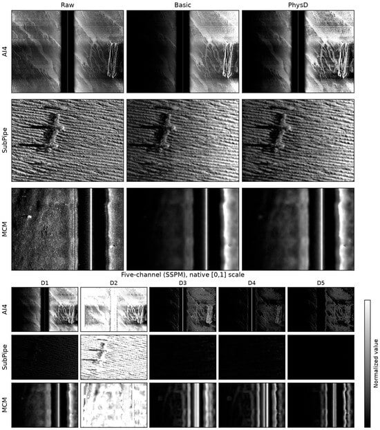
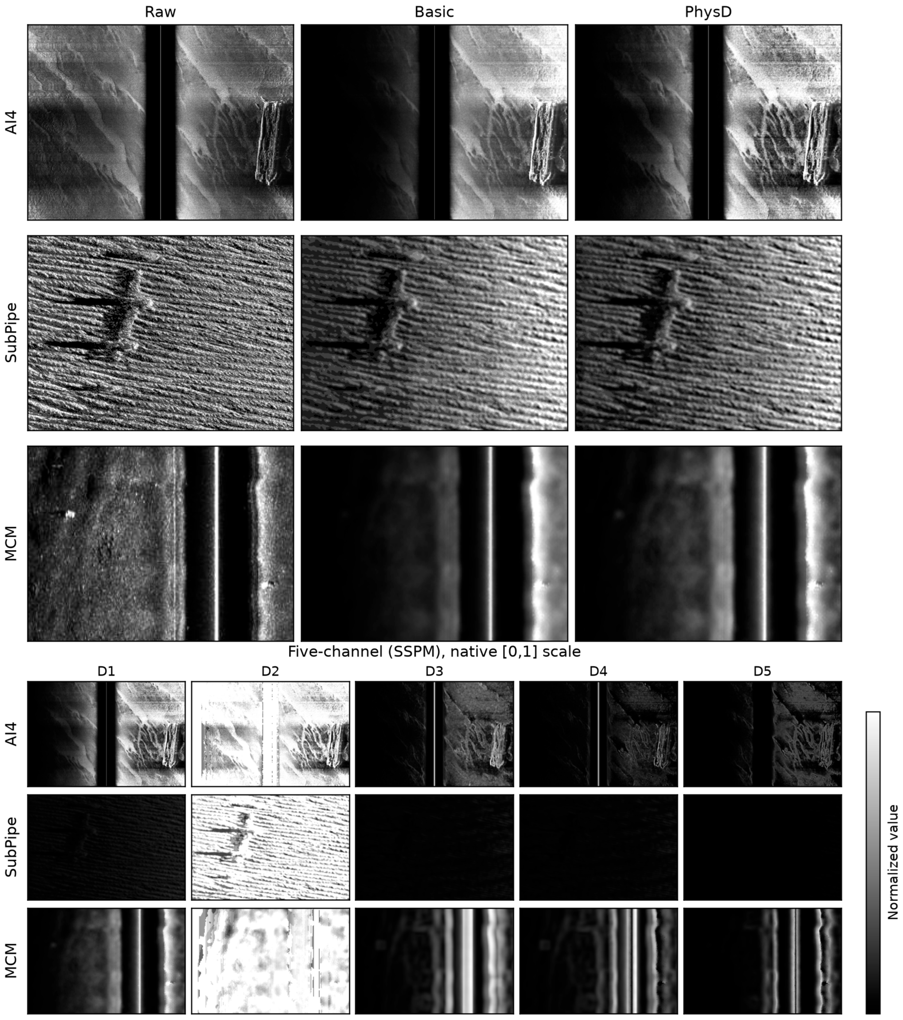
Figure 1 illustrates the four input representations compared in this study: Raw, Basic, PhysD, and five-channel inputs. The five-channel representation is constructed by the Structure-enhanced Sonar Preprocessing Module (SSPM), which derives five descriptors from PhysD and maps them to the encoder through a learnable stem. Let u denote PhysD intensity normalized to [0, 1]. The descriptor maps are denoted by $D_i$.

Figure 1. Input representations compared in this study: Raw, Basic, PhysD, and the five SSPM descriptor maps (D1–D5). D1–D5 are the outputs of Equations (7)–(11) and are displayed on a common [0, 1] color scale. Raw, Basic, and PhysD use separate 1st–99th percentile stretches for visualization. Descriptor statistics are computed over each full image before the displayed windows are extracted.

The first descriptor retains the normalized intensity:

$$D_1=u.$$

(7)

The second rescales intensity by the median of the corresponding image column:

$$D_2=\mathrm{c}\mathrm{l}\mathrm{i}\mathrm{p}\left({\displaystyle \frac{u}{\mathrm{m}\mathrm{a}\mathrm{x}\left({\mathrm{m}\mathrm{e}\mathrm{d}\mathrm{i}\mathrm{a}\mathrm{n}}_{\mathrm{c}\mathrm{o}\mathrm{l}}\right(u),{10}^{-6})}},0,1\right).$$

(8)

Local intensity variation is represented by the standard deviation within a reflect-padded 15 × 15 window:

$$D_3={\displaystyle \frac{{\sigma }_{15\times 15}\left(u\right)}{\mathrm{m}\mathrm{a}\mathrm{x}\left({\sigma }_{15\times 15}\left(u\right)\right)+ϵ}}.$$

(9)

A shadow-related descriptor combines low intensity with local variation:

$$D_4={\displaystyle \frac{(1-u)D_3}{\mathrm{m}\mathrm{a}\mathrm{x}\left((1-u)D_3\right)+ϵ}}.$$

(10)

The final descriptor combines local variation with a weighting function that emphasizes intermediate intensities:

$$D_5={\displaystyle \frac{D_3\mathrm{c}\mathrm{l}\mathrm{i}\mathrm{p}(1-2|u-0.5|,0,1)}{\mathrm{m}\mathrm{a}\mathrm{x}\left[D_3\mathrm{c}\mathrm{l}\mathrm{i}\mathrm{p}(1-2|u-0.5|,0,1)\right]+ϵ}}.$$

(11)

The maxima used to normalize $D_3$, $D_4$, and $D_5$ are calculated over the image. If a normalization maximum is zero, the corresponding descriptor is set to zero. The maps are concatenated along the channel dimension:

$$z_S=[D_1,D_2,D_3,D_4,D_5].$$

(12)

A 3 × 3 convolution followed by batch normalization and GELU maps the descriptors to three encoder channels:

$$F_0={\mathsf{\Psi }}_{\mathrm{s}\mathrm{t}\mathrm{e}\mathrm{m}}\left(z_S\right).$$

(13)

The comparison with PhysD evaluates the descriptor construction and learnable stem together; it does not isolate their individual contributions.

All statistics in Equations (8)–(11) are computed independently for each image over the full image, without an ignore mask or label information. The column medians in Equation (8) use all rows, and the maxima in Equations (9)–(11) use all pixels in the corresponding descriptor maps. The same procedure is applied to training, validation, and test images. No statistics are pooled across images or datasets, and no test-set statistics are used to normalize other images or the training data.

3.4. Segmentation Models

SegFormer-B2 is the principal architecture. Raw, Basic, and PhysD inputs are replicated across three channels. Five-channel input passes through ${\mathsf{\Psi }}_{\mathrm{s}\mathrm{t}\mathrm{e}\mathrm{m}}$.

The encoder generates hierarchical features

$$\{F_1,F_2,F_3,F_4\}=E_{{\theta }_e}\left(z_{\mathrm{e}\mathrm{n}\mathrm{c}}\right),$$

(14)

and the decoder produces semantic logits

$$Z=D_{{\theta }_d}(F_1,F_2,F_3,F_4), Z\in {\mathbb{R}}^{H\times W\times \left|\mathcal{C}\right|}.$$

(15)

Encoders are trained from random initialization without ImageNet pretraining.

FCN, U-Net, PSPNet, and DeepLabV3+ provide additional comparisons under a common soft-DMCE setting. Only SegFormer-B2 has a matched unmasked cross-entropy reference. The architecture experiment therefore provides a performance–cost profile under soft DMCE rather than a matched test of the objective for every architecture.

3.5. Dataset-Aware Masked Cross-Entropy

3.5.1. Dataset-Conditioned Logit Attenuation

A logit is a real-valued, unnormalized class score produced by the network before softmax. Let $h_p\in {\mathbb{R}}^D$ denote the feature vector supplied to the final $1\times 1$ classification convolution at location $p$. The raw logit for class $c$ is $Z_{p,c}=W_c^{\top }{h}_p+b_c,$ where $W_c$ and $b_c$ are the classifier weights and bias for that class. Before dataset-conditioned attenuation, these scores define the class probabilities, $P_{p,c}=\frac{\mathrm{e}\mathrm{x}\mathrm{p}\left(Z_{p,c}\right)}{{\sum }_{k\in C}\mathrm{e}\mathrm{x}\mathrm{p}\left(Z_{p,k}\right)}$. Thus, logits are not probabilities: they can take any real value, and their differences determine probability ratios, with $Z_{p,c}-Z_{p,k}=\mathrm{l}\mathrm{o}\mathrm{g}\left(P_{p,c}/P_{p,k}\right)$. In the implemented computation graph, the dataset-conditioned offset $\log {\alpha }_{d,c}$ is added directly to this logit tensor after the final classifier and before the softmax used to compute the training loss. No batch-normalization layer follows the final classifier, and no temperature scaling is applied; the training probabilities are computed using the standard softmax ($T=1$).

For dataset $d$ and class $c$, define the dataset-conditioned per-class attenuation factor

$${\alpha }_{d,c}=\left\{\begin{array}{ll}1,& c\in {\mathcal{V}}_d,\\ \rho ,& c\notin {\mathcal{V}}_d.\end{array}\right.$$

(16)

Here, ${\alpha }_{d,c}$ is determined by the annotation-supported set $V_d$ and the prescribed attenuation parameter $\rho \in \left(0,1\right]$; it is not learned. Supported classes receive a factor of 1, whereas unsupported classes receive a factor of $\rho$. The factor acts through the additive logit offset $\log {\alpha }_{d,c}$ in Equation (17), equivalently scaling the unnormalized exponential score in Equation (18).

At pixel $p$, the adjusted logits are

$${\tilde{Z}}_{p,c}=Z_{p,c}+\mathrm{l}\mathrm{o}\mathrm{g}{\alpha }_{d,c}.$$

(17)

The resulting training probabilities are

$${\tilde{P}}_{p,c}^{\left(d\right)}={\displaystyle \frac{{\alpha }_{d,c}\mathrm{e}\mathrm{x}\mathrm{p}\left(Z_{p,c}\right)}{{\sum }_{k\in \mathcal{C}}{\alpha }_{d,k}\mathrm{e}\mathrm{x}\mathrm{p}\left(Z_{p,k}\right)}}.$$

(18)

The evaluated objectives are:

• Unmasked cross-entropy: $\rho =1$.
• Soft DMCE: with $\rho =0.1$ used for the principal comparison unless otherwise stated.
• Hard masking: the limit $\rho \to 0$, implemented by adding a finite offset of $-{10}^9$ to unsupported-class logits and leaving supported-class logits unchanged.

For soft DMCE, unsupported logits receive an offset $\mathrm{l}\mathrm{o}\mathrm{g}\left(0.1\right)\approx -2.303$. This multiplies their unnormalized exponential scores by 0.1. It does not generally reduce their final normalized probabilities by exactly a factor of ten because the denominator also changes.

In the ideal hard-mask limit, unsupported classes have zero probability, corresponding to an offset $\log \rho \to -\infty$. The implementation uses −10⁹ as a finite numerical surrogate for this limit in float32. Its magnitude is intended to make unsupported-class logits sufficiently smaller than the retained logits that their exponential contributions vanish in floating-point evaluation. The constant is an implementation choice for approximating hard exclusion, rather than an attenuation strength selected through a performance search. Hard masking approximates exclusion of unsupported classes from the training normalization. Soft masking retains their probability contribution and, at fixed raw logits, reduces their suppressive gradients relative to unmasked cross-entropy.

3.5.2. Weighted Objective

For a training mini-batch of $B=4$ images drawn from a single dataset $d$, let $p$ index all pixel instances across the mini-batch, including the image index and the within-image pixel location. The supervised pixels are

$${\mathsf{\Omega }}_d=\left\{p:y_p\ne 255, y_p\in {\mathcal{V}}_d\right\}.$$

(19)

A supervised pixel is a pixel whose mapped label is not 255 and belongs to the annotation-supported set $V_d$; these pixels constitute ${\mathsf{\Omega }}_d$ and contribute to the training loss. Ignore-index pixels have the reserved label value 255, indicating that they cannot be mapped reliably to a shared class. They are excluded from both the numerator and denominator of Equation (21) and from all evaluation metrics.

Unless otherwise specified in the class-weight sensitivity analysis in Section 5.2, the class weights are

$$w_c=\left\{\begin{array}{ll}0.1,& c=c_0,\\ 3.0,& c\in \{c_1,c_2,c_3\}.\end{array}\right.$$

(20)

These weights were selected a priori as heuristic settings to increase the relative contribution of foreground pixels to the training loss. They were fixed before test evaluation and were not tuned using validation or test performance.

The objective is

$${\mathcal{L}}_{\mathrm{D}\mathrm{M}\mathrm{C}\mathrm{E}}=-{\displaystyle \frac{{\sum }_{p\in {\mathsf{\Omega }}_d}{w}_{y_p}\mathrm{l}\mathrm{o}\mathrm{g}{\tilde{P}}_{p,y_p}^{\left(d\right)}}{{\sum }_{p\in {\mathsf{\Omega }}_d}{w}_{y_p}}}.$$

(21)

The sums in Equation (21) are computed jointly over all supervised pixels in the mini-batch, yielding one scalar loss per batch. Unmasked, soft-masked, and hard-masked training use the same class weights and weighted reduction in the objective comparisons in Section 5.1. Holding these settings fixed separates the effect of logit attenuation from changes in class weighting.

Multiplying every $w_c$ by the same positive constant leaves Equation (21) unchanged because this factor cancels between the numerator and denominator. Changing the foreground-to-background weight ratio changes the relative contributions of supervised pixels. Section 5.2 examines this sensitivity by fixing the background weight at 0.1 and varying the common foreground weight over {1.0, 3.0, 6.0}.

3.5.3. Local Gradient Effect

For a supervised pixel,

$${\displaystyle \frac{\mathsf{\partial }\mathcal{L}}{\mathsf{\partial }{Z}_{p,c}}}={\displaystyle \frac{w_{y_p}}{{\sum }_{p\in {\mathsf{\Omega }}_d}{w}_{y_p}}}\left({\tilde{P}}_{p,c}^{\left(d\right)}-1[c=y_p]\right).$$

(22)

Equation (22) gives the derivative of the weighted loss in Equation (21) with respect to the raw logit $Z_{p,c}$. The indicator $1\left[c=y_p\right]$ equals 1 for the mapped target class and 0 otherwise. The gradient is the adjusted probability minus this target indicator, scaled by the target-class weight $w_{y_p}$ divided by the total supervised-pixel weight in the mini-batch. At the logit level, gradient descent therefore increases the target-class logit and decreases non-target-class logits. Pixels excluded from ${\mathsf{\Omega }}_d$ have zero direct contribution to the loss gradient.

For an unsupported class $c\notin {\mathcal{V}}_d$, the class cannot be the mapped target, so

$$1[c=y_p]=0.$$

(23)

For soft DMCE with finite logits, the gradient for an unsupported class is positive and proportional to its adjusted probability, so gradient descent acts to suppress that logit. At fixed raw logits, soft attenuation reduces this suppression relative to unmasked cross-entropy, as quantified in Equation (25). This is a local gradient comparison, rather than a guarantee of improved performance after training.

Define

$$A_p=\sum _{k\in {\mathcal{V}}_d}\mathrm{e}\mathrm{x}\mathrm{p}\left(Z_{p,k}\right), B_p=\sum _{k\notin {\mathcal{V}}_d}\mathrm{e}\mathrm{x}\mathrm{p}\left(Z_{p,k}\right).$$

(24)

For an unsupported class, the ratio between its soft-masked and unmasked probabilities is

$${\displaystyle \frac{{\tilde{P}}_{p,c}^{\left(d\right)}}{P_{p,c}}}={\displaystyle \frac{\rho (A_p+B_p)}{A_p+\rho B_p}}<1,$$

(25)

for 0 < $\rho$ < 1 and $A_p$ > 0. For finite logits and a nonempty supported-class set ${\mathcal{V}}_d$, $A_p$ is strictly positive in exact arithmetic because each exponential term is positive. If explicit floating-point evaluation resulted in $A_p$ = 0 while $B_p$ > 0 because of underflow, the ratio would equal 1 and the strict inequality would become equality. This inequality characterizes the local effect of attenuation at fixed logits.

3.5.4. Inference

Masking is used only during training. Predictions are obtained from the original logits:

$${\widehat{y}}_p=\mathrm{a}\mathrm{r}\mathrm{g}\underset{c\in \mathcal{C}}{\mathrm{m}\mathrm{a}\mathrm{x}}{Z}_{p,c}.$$

(26)

All four categories compete at evaluation. The experiment therefore evaluates each training objective together with full-label-space inference. For hard masking in particular, this protocol creates a difference between training-time and inference-time class competition.

3.6. Training Strategies

Single-dataset training fits a separate model to each source using unmasked weighted cross-entropy. Each model is evaluated on the corresponding test partition.

Naive joint training pools the observed sources under the same unmasked objective. Soft DMCE and hard masking change the dataset-conditioned logit attenuation while retaining the same class weights.

Dataset-balanced sampling is evaluated separately. It changes source exposure rather than the per-sample probability normalization.

4. Experimental Protocol

4.1. Experimental Design

The principal setting uses SegFormer-B2, five-channel input, ordinary sampling, and the fixed class weights defined in Section 3.5. The experimental comparisons, evaluation metrics, and intended interpretations are summarized in Table 2.

Table 2. Experimental comparisons and their intended interpretations.

Research Objective	Experimental Comparison	Main Metrics	Interpretation
Joint pooling utility	Single-dataset vs. joint CE	Dataset and macro mIoU; foreground IoU	Characterization of the observed effect of naive pooling
Soft attenuation	Joint CE vs. soft DMCE	Five matched seeds in the principal setting	Characterization of soft attenuation in the principal configuration
Hard exclusion	Soft vs. hard masking	Macro mIoU under full-space inference	Characterization of complete unsupported-class exclusion
Representation and sampling dependence	Input and sampler comparisons	Macro and dataset-specific mIoU	Characterization of changes across evaluated configurations
Missing foreground supervision	Leave-one-dataset-out evaluation	Foreground and background IoU	Characterization of recognition without positive source labels

4.2. Repeated Runs

Most conditions use five seed values: $\{1, 2, 3, 42, 3407\}.$ The five-channel hard-mask condition was run twice for each of these five seed values. For every reported statistic, the two runs associated with the same seed were first averaged. The overall mean and sample standard deviation were then calculated from the resulting five seed-level means. The same aggregation rule is used for the pooled macro mIoU, dataset-level mIoU, class-level IoU, and foreground IoU values reported for this condition.

4.3. Optimization and Model Selection

Training uses AdamW with an initial learning rate of 10⁻⁴, weight decay of 10⁻⁴, and batch size 4. Cosine annealing reduces the learning rate toward 10⁻⁶ over a maximum of 100 epochs. Training stops after 20 epochs without validation improvement.

Representations are computed before augmentation and resizing to 512 × 512. Horizontal and vertical flips have probabilities 0.5 and 0.3. Brightness and contrast vary by up to ±20% with probability 0.5. Spatial transforms are applied jointly to images and labels, while intensity changes affect images only.

Validation and test images receive no random augmentation. Joint models are selected by validation macro mIoU across the observed sources. Separate models use their corresponding validation partitions. Test scores are calculated from the selected checkpoints.

4.4. Input and Masking Comparisons

Raw, Basic, PhysD, and five-channel inputs are compared using unmasked cross-entropy. The same backbone and decoder architecture is used across these comparisons, with an additional learnable input stem for the five-channel configuration. All comparisons use ordinary sampling, under which dataset selection follows each dataset’s share of the pooled training images.

Soft and hard masking are compared under PhysD and five-channel representations where results are available. The available experiments do not cover every combination of objective, representation, sampler, and architecture.

The five-channel change includes both descriptor construction and an additional learnable stem. It is therefore not an isolated test of individual handcrafted channels.

4.5. Dataset-Balanced Sampling

Ordinary sampling follows pooled image frequencies. Dataset-balanced sampling first selects a source uniformly and then samples an image from that source:

$$d\sim \mathrm{U}\mathrm{n}\mathrm{i}\mathrm{f}\mathrm{o}\mathrm{r}\mathrm{m}\left({\mathcal{S}}_{\mathrm{t}\mathrm{r}\mathrm{a}\mathrm{i}\mathrm{n}}\right), x\sim \mathrm{U}\mathrm{n}\mathrm{i}\mathrm{f}\mathrm{o}\mathrm{r}\mathrm{m}\left({\mathcal{D}}_d^{\mathrm{t}\mathrm{r}\mathrm{a}\mathrm{i}\mathrm{n}}\right).$$

(27)

Let $o\in \left\{\mathrm{C}\mathrm{E},\mathrm{D}\mathrm{M}\mathrm{C}\mathrm{E}\right\}$ denote the training objective, $a\in \left\{\mathrm{o}\mathrm{r}\mathrm{d}\mathrm{i}\mathrm{n}\mathrm{a}\mathrm{r}\mathrm{y},\mathrm{b}\mathrm{a}\mathrm{l}\mathrm{a}\mathrm{n}\mathrm{c}\mathrm{e}\mathrm{d}\right\}$ denote the sampling strategy, and $r$ index the matched training seed. We write $S_{o,a}^{\left(r\right)}$ for the test macro mIoU obtained with objective $o$, sampling strategy $a$, and seed $r$. The conditional sampling effect is

$${\Delta }_{\mathrm{s}\mathrm{a}\mathrm{m}\mathrm{p}\mathrm{l}\mathrm{i}\mathrm{n}\mathrm{g}\mid o}^{\left(r\right)}={S^{\left(r\right)}}_{o,\mathrm{b}\mathrm{a}\mathrm{l}\mathrm{a}\mathrm{n}\mathrm{c}\mathrm{e}\mathrm{d}}-{S^{\left(r\right)}}_{o,\mathrm{o}\mathrm{r}\mathrm{d}\mathrm{i}\mathrm{n}\mathrm{a}\mathrm{r}\mathrm{y}}.$$

(28)

Thus, ${\Delta }_{\mathrm{s}\mathrm{a}\mathrm{m}\mathrm{p}\mathrm{l}\mathrm{i}\mathrm{n}\mathrm{g}\mid o}^{\left(r\right)}$ is the conditional effect of changing the sampler while holding the objective and seed fixed. A positive value means that dataset-balanced sampling improves macro mIoU relative to ordinary pooled-frequency sampling for that objective and seed; a negative value means that it decreases macro mIoU.

The objective-sampling interaction is

$$I^{\left(r\right)}={{\Delta }^{\left(r\right)}}_{\mathrm{s}\mathrm{a}\mathrm{m}\mathrm{p}\mathrm{l}\mathrm{i}\mathrm{n}\mathrm{g}\mid \mathrm{D}\mathrm{M}\mathrm{C}\mathrm{E}}-{{\Delta }^{\left(r\right)}}_{\mathrm{s}\mathrm{a}\mathrm{m}\mathrm{p}\mathrm{l}\mathrm{i}\mathrm{n}\mathrm{g}\mid \mathrm{C}\mathrm{E}}.$$

(29)

Equation (29) is a difference-in-differences contrast. It measures whether the performance change produced by dataset-balanced sampling differs between the DMCE and CE objectives. In other words, it quantifies the extent to which the benefit or cost of changing the sampling strategy depends on the training objective. It is not the difference between the absolute performances of DMCE and CE; it is the difference between their sampler-induced performance changes. Under this sign convention, $I^{\left(r\right)}<0$ means that balanced sampling improves CE more than it improves DMCE for seed $r$. Conversely, $I^{\left(r\right)}>0$ means that balanced sampling improves DMCE more than CE, or harms DMCE less than CE. If $I^{\left(r\right)}$ is close to zero, the change from ordinary to balanced sampling is similar for the two objectives.

For each matched seed $r$, we first compute ${\Delta }_{\mathrm{s}\mathrm{a}\mathrm{m}\mathrm{p}\mathrm{l}\mathrm{i}\mathrm{n}\mathrm{g}\mid \mathrm{C}\mathrm{E}}^{\left(r\right)}$, ${\Delta }_{\mathrm{s}\mathrm{a}\mathrm{m}\mathrm{p}\mathrm{l}\mathrm{i}\mathrm{n}\mathrm{g}\mid \mathrm{D}\mathrm{M}\mathrm{C}\mathrm{E}}^{\left(r\right)}$, and $I^{\left(r\right)}$. We then summarize the five seed-level interaction values using their mean and sample standard deviation. Thus, the interaction is computed before aggregation, rather than by subtracting independently aggregated group means. In the five-seed comparison, the mean sampling improvement was +0.0271 for CE and +0.0146 for DMCE. Therefore, the mean interaction was $I$ = −0.0126, with a sample standard deviation of 0.0417. The negative mean indicates that balanced sampling improved CE more than DMCE on average under this configuration. However, the per-seed interaction values were +0.0293, −0.0583, +0.0084, +0.0144, and −0.0566, spanning both signs. We therefore interpret this result as a weak and seed-dependent interaction rather than as a strong or universal interaction between the objective and the sampling strategy. Here, the pooled image frequencies are the proportions of training images contributed by each source: 121/1219 (9.9%) for AI4, 558/1219 (45.8%) for MCM, and 540/1219 (44.3%) for SubPipe. These proportions describe source representation in the pooled training set; each mini-batch still contains images from only one dataset.

4.6. Evaluation Metrics

Ignore-index pixels are excluded. For supported class $c$ in dataset $d$,

$${\mathrm{I}\mathrm{o}\mathrm{U}}_{d,c}={\displaystyle \frac{{\mathrm{T}\mathrm{P}}_{d,c}}{{\mathrm{T}\mathrm{P}}_{d,c}+{\mathrm{F}\mathrm{P}}_{d,c}+{\mathrm{F}\mathrm{N}}_{d,c}}}.$$

(30)

A prediction outside ${\mathcal{V}}_d$ at a valid pixel counts as a false negative for its ground-truth class. It is not discarded or reassigned to background. Unsupported categories are omitted from that dataset’s class average.

Each source supports background and one foreground category:

$${\mathrm{m}\mathrm{I}\mathrm{o}\mathrm{U}}_d={\displaystyle \frac{{\mathrm{I}\mathrm{o}\mathrm{U}}_{d,\mathrm{B}\mathrm{G}}+{\mathrm{I}\mathrm{o}\mathrm{U}}_{d,\mathrm{F}\mathrm{G}}}{2}}.$$

(31)

Macro mIoU gives equal weight to the evaluated datasets:

$$M={\displaystyle \frac{1}{\left|{\mathcal{S}}_{\mathrm{e}\mathrm{v}\mathrm{a}\mathrm{l}}\right|}}\sum _{d\in {\mathcal{S}}_{\mathrm{e}\mathrm{v}\mathrm{a}\mathrm{l}}}{\mathrm{m}\mathrm{I}\mathrm{o}\mathrm{U}}_d.$$

(32)

Foreground macro-IoU is

$$M_{\mathrm{F}\mathrm{G}}={\displaystyle \frac{1}{\left|{\mathcal{S}}_{\mathrm{e}\mathrm{v}\mathrm{a}\mathrm{l}}\right|}}\sum _{d\in {\mathcal{S}}_{\mathrm{e}\mathrm{v}\mathrm{a}\mathrm{l}}}{\mathrm{I}\mathrm{o}\mathrm{U}}_{d,FG}.$$

(33)

Binary mIoU weights background and foreground equally. A value near 0.5 can therefore occur when background IoU approaches one and foreground IoU approaches zero. Binary mIoU must be interpreted together with foreground IoU.

4.7. Leave-One-Dataset-Out Evaluation Protocol

Each leave-one-dataset-out experiment trains on two sources and evaluates the excluded third source:

$${\mathcal{D}}_{\mathrm{s}\mathrm{o}\mathrm{u}\mathrm{r}\mathrm{c}\mathrm{e}}^{\mathrm{t}\mathrm{r}\mathrm{a}\mathrm{i}\mathrm{n}}=\bigcup _{d\ne d_t}{\mathcal{D}}_d^{\mathrm{t}\mathrm{r}\mathrm{a}\mathrm{i}\mathrm{n}},$$

(34)

where $d_t$ is the excluded dataset.

Checkpoint selection uses source validation partitions only. Excluded labels do not contribute to optimization or model selection.

Excluding a source also removes the only positive annotations for its foreground category. The experiment therefore combines acoustic distribution shift and missing category supervision.

4.8. Computational Evaluation

FCN, U-Net, PSPNet, DeepLabV3+, and SegFormer-B2 are compared under soft DMCE using common partitions, five-channel input, ordinary sampling, and the same training limits. SegFormer-B2 additionally has an unmasked reference.

Parameters, floating-point operations, latency, and frames per second are reported. FLOPs are defined as twice the multiply-accumulate count.

Timing was performed on an NVIDIA Jetson Orin platform using 14 software threads. The model input was a CPU tensor with shape $1\times 5\times 512\times 512$ and a batch size of 1. For model-forward latency, five warm-up iterations preceded 30 timed iterations. Latency covers the complete network forward pass, model(x), and excludes image reading, PhysD computation, resizing, SSPM construction, and post-processing. Because both the model and input were on the CPU, no CPU-to-GPU transfer was involved. Forward FPS was calculated as $1000$ divided by the mean forward latency in milliseconds and represents model-only throughput rather than end-to-end processing rate.

Preprocessing latency was measured separately for image reading, PhysD computation, resizing to $512\times 512$, and SSPM construction, using 10 test images per dataset. The preprocessing-inclusive input-image-to-logit time is estimated by adding the dataset-specific mean preprocessing latency to the mean model-forward latency. It excludes sonar acquisition and all post-processing after the network forward pass, including conversion of logits to discrete labels by argmax. Therefore, it does not represent acquisition-to-final-segmentation time.

4.9. Statistical Analysis

Dataset metrics are combined into a macro score within each run. Means and sample standard deviations are then calculated across runs. Macro standard deviation is not obtained by averaging dataset-level standard deviations.

Matched five-seed comparisons use exact Wilcoxon signed-rank tests, with two-sided tests treated as primary and one-sided tests treated as exploratory. With five nonzero pairs, the minimum attainable one-sided and two-sided p-values are 0.03125 and 0.0625, respectively. Therefore, a two-sided p-value of 0.0625 is not significant at the 0.05 level. Holm correction was applied across the three matched attenuation comparisons reported in Section 5.1; no comparison remained significant at the 0.05 level after correction.

The Wilcoxon signed-rank test is a non-parametric test for paired observations. We pair results by training seed and rank the absolute nonzero differences between methods, retaining their signs. The test evaluates the null hypothesis that the distribution of paired differences is symmetric about zero. The exact two-sided p-value is the probability, under this null hypothesis, of obtaining a signed-rank statistic at least as extreme as the observed one in either direction. With five nonzero pairs, the smallest attainable exact two-sided p-value is 0.0625, so this test cannot reach the 0.05 significance level with the current number of pairs.

The statistical unit is the training run, not the pixel. Repeated training under fixed partitions describes optimization variability rather than uncertainty across independent sonar surveys or alternative dataset splits.

5. Results

5.1. Joint Training and Dataset-Aware Masking

The aggregate hard-masked performance is reported in Table 3. The run-level variability of the hard-masked condition is reported in Table 4. The mean absolute difference between the two runs within a seed was approximately 0.133 macro mIoU, with individual differences ranging from 0.0404 to 0.2376. A one-way random-effects analysis estimated a raw between-seed variance component of −0.001733 and a within-seed variance component of 0.012439; the negative between-seed estimate was truncated to zero. The two runs associated with each seed were averaged before calculating the mean and sample standard deviation across the five seed-level values.

Table 3. Single-dataset and joint-training performance.

Training Strategy	AI4 mIoU	MCM mIoU	SubPipe mIoU	Foreground Macro-IoU, ${\mathit{M}}_{\mathbf{F}\mathbf{G}}$	Macro mIoU
Single-dataset training	0.5675 ± 0.0265	0.5474 ± 0.0370	0.4881 ± 0.0124	0.0923 ± 0.0380	0.5343 ± 0.0224
Naive joint training	0.5656 ± 0.0599	0.5093 ± 0.0325	0.4952 ± 0.0027	0.0694 ± 0.0413	0.5234 ± 0.0303
Soft DMCE joint training	0.5063 ± 0.0498	0.4734 ± 0.0597	0.4928 ± 0.0044	0.0409 ± 0.0360	0.4908 ± 0.0353
Hard-masked joint training	0.1752 ± 0.0851	0.1056 ± 0.0849	0.1825 ± 0.0464	0.0144 ± 0.0153	0.1544 ± 0.0670

Note: Values are means ± sample standard deviations across five seed-level values. $M_{\mathrm{F}\mathrm{G}}$ is the arithmetic mean of the IoUs for the three dataset-specific foreground classes (AI4: C1, MCM: C3, and SubPipe: C2); background and unsupported classes are excluded. For the hard-mask condition, the two runs associated with each seed were first averaged. The reported mean and sample standard deviation were then calculated from the five resulting seed-level values using $n-1$ in the denominator. Bold identifies the highest reported mean in each column.

Table 4. Run-level variability of hard-masked joint training.

Seed	Run 1 Macro mIoU	Run 2 Macro mIoU	Seed-Level Mean	Absolute Within-Seed Difference
1	0.1344	0.0498	0.0921	0.0846
2	0.2342	0.2746	0.2544	0.0404
3	0.0295	0.2630	0.1463	0.2335
42	0.0634	0.1316	0.0975	0.0682
3407	0.0631	0.3007	0.1819	0.2376
Mean	—	—	0.1544	0.1329

Note: The two runs associated with each seed were averaged to obtain the seed-level means. The mean absolute difference between the paired runs was approximately 0.133 macro mIoU, with individual differences ranging from 0.0404 to 0.2376. A one-way random-effects model was fitted to the 10 run-level observations using seed as the grouping factor. The raw between-seed variance-component estimate was −0.001733, and the within-seed variance-component estimate was 0.012439. The negative between-seed estimate was truncated to zero for the non-negative variance summary. These variance-component estimates are reported descriptively; the hard-mask results in Table 3 use the prespecified seed-level aggregation rule, in which the two runs for each seed are averaged before calculating the across-seed mean and sample standard deviation.

Because dataset-level mIoU averages background and foreground IoU, we also report the foreground-only aggregate $M_{\mathrm{F}\mathrm{G}}$ in Table 3. The values were 0.0923 ± 0.0380 for single-dataset training, 0.0694 ± 0.0413 for naive joint training, 0.0409 ± 0.0360 for soft DMCE, and 0.0144 ± 0.0153 for hard-masked joint training. These values provide the target-recognition results that are not visible in the background-inclusive macro mIoU.

Separate models achieved a macro mIoU of 0.5343, compared with 0.5234 for naive joint training. The single-dataset means were higher by 0.0019 on AI4 and 0.0381 on MCM, while naive joint training was higher by 0.0071 on SubPipe. The direction therefore varied across datasets, and the aggregate comparison did not show a consistent advantage for naive pooling.

Soft DMCE reduced macro mIoU by 0.0326 relative to naive joint cross-entropy. All five paired macro-mIoU differences were negative. The exact two-sided Wilcoxon signed-rank test gave $p=0.0625$, the smallest attainable two-sided exact p-value for five nonzero paired differences; the exploratory one-sided test in the observed direction gave $p=0.03125$. After Holm correction across the three matched attenuation comparisons in Table 5, the adjusted p-value for the $\rho =0.1$ comparison was 0.1875.

Table 5. Joint-training performance across attenuation settings.

Objective	$\mathit{\rho }$	Unsupported-Class Offset $\mathbf{log}\mathit{\rho }$	Macro mIoU, Mean ± SD	Foreground Macro-IoU, Mean ± SD	Δ Macro mIoU vs. CE	Raw Paired Two-Sided $\mathit{p}$	Holm-Adjusted $\mathit{p}$
Cross-entropy	1.00	0	0.5234 ± 0.0303	0.0694 ± 0.0413	—	—	—
Soft DMCE	0.50	−0.693	0.5134 ± 0.0309	0.0530 ± 0.0444	−0.0100	0.4375	0.4375
Soft DMCE	0.10	−2.303	0.4908 ± 0.0353	0.0409 ± 0.0360	−0.0326	0.0625	0.1875
Soft DMCE	0.01	−4.605	0.4771 ± 0.0252	0.0339 ± 0.0251	−0.0463	0.0625	0.1875

Note: Values are means ± sample standard deviations across five seed-level values. Each sample standard deviation is calculated as the square root of the sum of squared deviations from the mean divided by $n-1$, where $n=5$. $M_{\mathrm{F}\mathrm{G}}$ is the arithmetic mean of the IoUs for the three dataset-specific foreground classes (AI4: C1, MCM: C3, and SubPipe: C2); background and unsupported classes are excluded. The raw $p$-values are exact two-sided Wilcoxon signed-rank test results for the three matched attenuation comparisons against the cross-entropy reference. Holm adjustment was applied across these three comparisons as one multiplicity family. None of the comparisons reached the 0.05 significance level before or after Holm correction. The one-sided tests were exploratory and are not reported in this table.

Hard masking produced a macro mIoU of 0.1544 ± 0.0670, substantially below both unmasked cross-entropy and soft DMCE. The two runs associated with each seed were averaged before the hard-mask mean and sample standard deviation were calculated across the five seed-level values, as specified in Table 3 and detailed in Table 4.

The effect of attenuation strength is summarized in Table 5. With the same SegFormer-B2, five-channel input, ordinary sampling, and fixed class weights, mean macro mIoU was 0.5234 for the unmasked cross-entropy reference and 0.5134, 0.4908, and 0.4771 for soft DMCE with $\rho =0.5$, 0.1, and 0.01, respectively. Foreground macro-IoU followed the same ordering, with means of 0.0694, 0.0530, 0.0409, and 0.0339. The macro-mIoU difference from cross-entropy was negative in 4/5 seeds for $\rho =0.5$ and in all five seeds for $\rho =0.1$ and 0.01. The corresponding paired two-sided exact Wilcoxon signed-rank tests gave $p=0.4375$, 0.0625, and 0.0625, respectively. After Holm correction across the three matched attenuation comparisons, the adjusted p-values were 0.4375, 0.1875, and 0.1875, respectively. All three tested finite attenuation settings therefore had lower mean macro mIoU than the unmasked cross-entropy reference, although none of the paired two-sided comparisons reached the 0.05 level before or after correction. The PhysD comparison in Section 5.3 showed the opposite objective ordering.

5.2. Foreground-Specific Performance

At the default foreground weight of 3.0, naive joint training achieved a higher mean IoU than soft DMCE for all three foreground categories. Shipwreck IoU decreased from 0.1546 to 0.0835, pipeline IoU from 0.0013 to 0.0006, and mine-like-contact IoU from 0.0523 to 0.0387. Hard masking yielded shipwreck, pipeline, and mine-like-contact IoUs of 0.0233, 0.0030, and 0.0169, respectively. Although its pipeline IoU was higher than those of the other joint-training objectives, its foreground mean was the lowest, at 0.0144. The dataset-specific foreground IoU values are reported in Table 6.

Table 6. Dataset-specific foreground IoU.

Training Strategy	Shipwreck IoU	Pipeline IoU	Mine-like-Contact IoU	Foreground Mean
Single-dataset training	0.1651	0.0051	0.1066	0.0923
Naive joint training	0.1546	0.0013	0.0523	0.0694
Soft DMCE joint training	0.0835	0.0006	0.0387	0.0409
Hard-masked joint training	0.0233	0.0030	0.0169	0.0144

Note: Entries are means across five seed-level values. Shipwreck, pipeline, and mine-like-contact IoUs are evaluated on AI4, SubPipe, and MCM, respectively. The foreground mean is the arithmetic mean of these three dataset-specific foreground IoUs. For hard-masked training, the two repeated runs associated with each seed are averaged before aggregation across seeds.

Pipeline IoU was close to zero even under single-dataset training. Consequently, a SubPipe binary mIoU near 0.5 does not indicate useful pipeline segmentation. It can arise from near-perfect background overlap combined with negligible foreground overlap. The same pattern is also evident under hard masking.

To examine how class weighting affects the objective comparison, we fixed the background weight at 0.1 and varied the common foreground weight over $\left\{1.0,3.0,6.0\right\}$, corresponding to foreground-to-background weight ratios of $10:1$, $30:1$, and $60:1$. At each setting, unmasked CE and soft DMCE with $\rho =0.1$ were evaluated using the same five training seeds. All configurations used SegFormer-B2, five-channel SSPM inputs, ordinary sampling, and the same data splits, training settings, and evaluation procedure as Table 3. The results at a foreground weight of 3.0 were reused from the main objective comparison, and 20 additional training runs were completed for the other two weights. Table 7 summarizes the results.

Table 7. Sensitivity of joint-training performance to the foreground class weight.

Foreground Weight ${\mathit{w}}_{\mathbf{f}\mathbf{g}}$	Foreground:Background Ratio	Training Objective	Macro mIoU	Foreground Macro-IoU
1.0	10:1	Unmasked CE	0.5462 ± 0.0215	0.1000 ± 0.0414
1.0	10:1	Soft DMCE	0.5214 ± 0.0342	0.0571 ± 0.0625
3.0	30:1	Unmasked CE	0.5234 ± 0.0303	0.0694 ± 0.0413
3.0	30:1	Soft DMCE	0.4908 ± 0.0353	0.0409 ± 0.0360
6.0	60:1	Unmasked CE	0.4907 ± 0.0229	0.0207 ± 0.0204
6.0	60:1	Soft DMCE	0.4674 ± 0.0484	0.0293 ± 0.0398

Note: Values are means ± sample standard deviations across five training seeds. The background weight is fixed at 0.1, and all foreground classes share the listed foreground weight. Soft DMCE uses $\rho =0.1$. Macro mIoU includes background, whereas foreground macro-IoU averages the three dataset-specific foreground IoUs defined in Table 6. Results at $w_{\mathrm{f}\mathrm{g}}=3.0$ are reused from the objective comparison in Table 3.

Unmasked CE achieved higher mean macro mIoU than soft DMCE at all three foreground weights. The CE-minus-soft-DMCE differences were 0.0248, 0.0326, and 0.0233 at weights 1.0, 3.0, and 6.0, respectively. The mean macro-mIoU ordering observed in Table 3 therefore persisted across the three tested weight ratios.

Absolute performance changed with the weight setting. For both objectives, mean macro mIoU and foreground macro IoU decreased as the foreground weight increased across the tested values. Both objectives achieved their highest mean values at a foreground weight of 1.0. Foreground macro IoU also showed a change in objective ordering: unmasked CE was higher at weights 1.0 and 3.0, whereas soft DMCE was higher at a weight of 6.0, with values of 0.0293 versus 0.0207. These results distinguish a consistent mean macro-mIoU ordering from a foreground-performance ordering that depends on the class-weight ratio.

5.3. Input Representation

Raw input obtained the highest reported mean on every dataset. Its macro mIoU was 0.5331, followed by Basic at 0.5242, five-channel input at 0.5234, and PhysD at 0.4952.

Five-channel input exceeded PhysD by 0.0282 but remained 0.0097 below Raw. The difference relative to PhysD was concentrated on AI4 and MCM, while the SubPipe means were identical to four decimal places. The results for the four input representations are summarized in Table 8.

Table 8. Input comparison under unmasked joint cross-entropy.

Input Representation	AI4 mIoU	MCM mIoU	SubPipe mIoU	Macro mIoU
Raw	0.5776 ± 0.0431	0.5240 ± 0.0211	0.4976 ± 0.0008	0.5331 ± 0.0190
Basic	0.5645 ± 0.0461	0.5130 ± 0.0162	0.4951 ± 0.0029	0.5242 ± 0.0197
PhysD	0.5090 ± 0.0402	0.4814 ± 0.0305	0.4952 ± 0.0040	0.4952 ± 0.0215
Five-channel	0.5656 ± 0.0599	0.5093 ± 0.0325	0.4952 ± 0.0027	0.5234 ± 0.0303

Note: Values are means ± sample standard deviations over five seeds. All rows use SegFormer-B2, ordinary sampling, and the same weighted cross-entropy objective.

Five-channel input improved macro mIoU from 0.4952 with PhysD to 0.5234, but remained below Raw input at 0.5331. The experiment evaluates the descriptor set and learnable stem jointly. Under PhysD input, soft DMCE achieved macro mIoU 0.5204, compared with 0.4952 for unmasked cross-entropy. Hard masking under PhysD achieved 0.2854.

Thus, the ordering of soft DMCE and cross-entropy changed between PhysD and five-channel inputs. Because the PhysD comparison was not evaluated with a paired significance test, this result is reported descriptively.

5.4. Training Objective and Dataset Sampling

Dataset-balanced sampling increased the cross-entropy macro mIoU from 0.5234 to 0.5505 and the foreground macro IoU, $M_{\mathrm{F}\mathrm{G}}$, from 0.0694 ± 0.0413 to 0.1138 ± 0.0144. The largest dataset-specific gain occurred on AI4, the smallest training source; MCM also improved, whereas SubPipe changed little. The paired macro-mIoU difference was positive in all five seeds. The primary exact two-sided Wilcoxon signed-rank test gave $p=0.0625$, which does not reach the 0.05 significance level. The one-sided result ($p=0.03125$) is exploratory and is not used to claim statistical significance. The objective-sampling results are summarized in Table 9.

Table 9. Objective-sampling comparison.

Objective	Sampler	AI4 mIoU	MCM mIoU	SubPipe mIoU	Foreground Macro-IoU, ${\mathit{M}}_{\mathbf{F}\mathbf{G}}$	Macro mIoU
Cross-entropy	Ordinary	0.5656 ± 0.0599	0.5093 ± 0.0325	0.4952 ± 0.0027	0.0694 ± 0.0413	0.5234 ± 0.0303
Cross-entropy	Dataset-balanced	0.6226 ± 0.0344	0.5331 ± 0.0277	0.4959 ± 0.0022	0.1138 ± 0.0144	0.5505 ± 0.0078
Soft DMCE	Ordinary	0.5063 ± 0.0498	0.4734 ± 0.0597	0.4928 ± 0.0044	0.0409 ± 0.0360	0.4908 ± 0.0353
Soft DMCE	Dataset-balanced	0.5589 ± 0.0617	0.4652 ± 0.0626	0.4921 ± 0.0118	0.0670 ± 0.0395	0.5054 ± 0.0403

Note: Values are means ± sample standard deviations over five seeds. $M_{\mathrm{F}\mathrm{G}}$ is calculated for each seed as the arithmetic mean of the IoUs for the three dataset-specific foreground classes; background and unsupported classes are excluded. For the cross-entropy comparison between dataset-balanced and ordinary sampling, the exact two-sided Wilcoxon signed-rank test gave $p=0.0625$, which is not statistically significant at the 0.05 level. The one-sided result ($p=0.03125$) is exploratory and is not used to claim statistical significance. Bold identifies the highest reported mean in each column.

Under soft DMCE, balanced sampling increased the macro mIoU from 0.4908 to 0.5054 and $M_{\mathrm{F}\mathrm{G}}$ from 0.0409 ± 0.0360 to 0.0670 ± 0.0395. The paired macro-mIoU difference was positive in three of five seeds, with a reported exploratory one-sided value of p = 0.5000. AI4 improved, while MCM and SubPipe decreased slightly.

Soft DMCE remained below cross-entropy under both samplers. The mean objective differences were 0.0326 under ordinary sampling and 0.0451 under balanced sampling.

The seed-level interaction was $I=-0.0126\pm 0.0417$.

Three interaction values were positive and two were negative. The sampling-objective interaction was inconsistent across seeds, with three positive and two negative values. Minor discrepancies between calculations based on displayed table values and the reported interaction arise from rounding.

5.5. Held-Out Evaluation Under Missing Foreground Supervision

Foreground IoU was zero in every held-out condition. The reported mIoU values therefore equal approximately half of the corresponding background IoU. The held-out results are summarized in Table 10.

Table 10. Held-out performance when the excluded dataset supplies the only positive foreground annotations.

Held-Out Dataset	Training Datasets	Objective	mIoU	Foreground IoU	Background IoU
AI4	MCM + SubPipe	Cross-entropy	0.4784 ± 0.0067	0.0000 ± 0.0000	0.9567 ± 0.0134
AI4	MCM + SubPipe	Soft DMCE	0.4674 ± 0.0218	0.0000 ± 0.0000	0.9349 ± 0.0435
MCM	AI4 + SubPipe	Cross-entropy	0.4436 ± 0.0747	0.0000 ± 0.0000	0.8872 ± 0.1494
MCM	AI4 + SubPipe	Soft DMCE	0.4585 ± 0.0214	0.0000 ± 0.0000	0.9171 ± 0.0427
SubPipe	AI4 + MCM	Cross-entropy	0.4972 ± 0.0012	0.0000 ± 0.0000	0.9944 ± 0.0023
SubPipe	AI4 + MCM	Soft DMCE	0.4936 ± 0.0101	0.0000 ± 0.0000	0.9871 ± 0.0202

Note: Values are means ± sample standard deviations over five seeds. Checkpoints are selected using source validation data only.

Soft DMCE had a lower mean mIoU on held-out AI4 and SubPipe and a higher mean on held-out MCM. Because neither objective produced foreground overlap, these differences describe background prediction rather than recognition of the excluded category.

Attenuating negative supervision alone did not provide the positive semantic evidence required for recognition of the excluded category. Acoustic and annotation distribution shifts are also present in this setting.

5.6. Architecture and Computational Profile

Among the architectures evaluated under soft DMCE, FCN achieved the highest $M_{\mathrm{F}\mathrm{G}}$ (0.1221 ± 0.0167) and the highest macro mIoU (0.5576 ± 0.0085). PSPNet achieved the highest AI4 mean and the lowest model-forward latency at 235.8 ms. The foreground-specific results provide a complementary view of performance: $M_{\mathrm{F}\mathrm{G}}$ was 0.1025 ± 0.0336 for PSPNet, 0.0871 ± 0.0257 for DeepLabV3+, and 0.0416 ± 0.0234 for U-Net. The segmentation and computational results for the evaluated architectures are summarized in Table 11.

Table 11. Segmentation performance and computational cost across architectures.

Architecture	Objective	AI4 mIoU	MCM mIoU	SubPipe mIoU	Foreground Macro IoU, ${\mathit{M}}_{\mathbf{F}\mathbf{G}}$	Macro mIoU	Parameters (M)	FLOPs (G)	Latency (ms)	Forward FPS
FCN	Soft DMCE	0.5724 ± 0.0261	0.6023 ± 0.0165	0.4979 ± 0.0004	0.1221 ± 0.0167	0.5576 ± 0.0085	35.32	297.95	1311.2 ± 35.6	0.76
U-Net	Soft DMCE	0.4878 ± 0.0049	0.5516 ± 0.0417	0.4964 ± 0.0031	0.0416 ± 0.0234	0.5119 ± 0.0127	28.95	388.59	1539.1 ± 41.5	0.65
PSPNet	Soft DMCE	0.5830 ± 0.0461	0.5639 ± 0.0100	0.4981 ± 0.0000	0.1025 ± 0.0336	0.5483 ± 0.0174	24.34	24.80	235.8 ± 11.0	4.24
DeepLabV3+	Soft DMCE	0.5541 ± 0.0297	0.5579 ± 0.0171	0.4980 ± 0.0005	0.0871 ± 0.0257	0.5367 ± 0.0132	39.64	329.07	1449.5 ± 35.3	0.69
SegFormer-B2	Cross-entropy	0.5656 ± 0.0599	0.5093 ± 0.0325	0.4952 ± 0.0027	0.0694 ± 0.0413	0.5234 ± 0.0303	24.72	42.65	647.1 ± 26.8	1.55
SegFormer-B2	Soft DMCE	0.5063 ± 0.0498	0.4734 ± 0.0597	0.4928 ± 0.0044	0.0409 ± 0.0360	0.4908 ± 0.0353	24.72	42.65	647.1 ± 26.8	1.55

Note: Segmentation results are reported as means ± sample standard deviations over five seeds. Forward latency and forward FPS were measured using the same hardware, batch size, and input shape for all architectures. Forward FPS is calculated as $1000/\mathrm{mean} \mathrm{forward} \mathrm{latency} \left(\mathrm{ms}\right)$. It excludes preprocessing and post-processing. The soft-DMCE architecture comparison provides a performance–cost profile; SegFormer-B2 is additionally reported with cross-entropy to provide a matched objective comparison.

FCN’s mean model-forward latency was 1311.2 ms, compared with 235.8 ms for PSPNet. Thus, FCN achieved the highest aggregate segmentation means, while PSPNet had the lowest model-forward latency among the evaluated architectures.

For SegFormer-B2, soft DMCE reduced both macro mIoU and $M_{\mathrm{F}\mathrm{G}}$ relative to cross-entropy (0.0409 ± 0.0360 vs. 0.0694 ± 0.0413 for $M_{\mathrm{F}\mathrm{G}}$), without changing inference cost. Only SegFormer-B2 includes a matched unmasked cross-entropy control; objective-level comparisons are therefore restricted to this architecture. The per-image preprocessing measurements are reported in Table 12.

Table 12. Per-image preprocessing latency by dataset (ms).

Dataset	n	Read	PhysD	Resize512	SSPM Construction	Preprocessing Total
AI4	10	38.4 ± 5.7	107.0 ± 7.3	0.5 ± 0.0	9.5 ± 1.5	155.5
SubPipe	10	5.1 ± 0.5	90.7 ± 3.4	0.8 ± 0.0	7.9 ± 0.4	104.4
MCM	10	1.5 ± 0.1	9.9 ± 0.2	0.3 ± 0.0	7.9 ± 0.6	19.5

Note: Stage timings are means ± standard deviations over 10 test images per dataset. Preprocessing totals were calculated from unrounded stage means and may differ slightly from the sum of displayed rounded values. The equal-dataset mean preprocessing time across AI4, SubPipe, and MCM was 93.1 ms.

Combining these dataset-specific preprocessing measurements with the model-forward latency yields the stored-image-to-logit processing estimates reported in Table 13.

Table 13. Estimated stored-image-to-logit processing time across architectures.

Architecture	Forward Latency (ms)	AI4 Total (ms)	SubPipe Total (ms)	MCM Total (ms)	Equal-Dataset Mean Total (ms)	Equal-Dataset FPS
FCN	1311.2	1466.7	1415.6	1330.7	1404.3	0.71
U-Net	1539.1	1694.6	1643.5	1558.6	1632.2	0.61
PSPNet	235.8	391.3	340.2	255.3	328.9	3.04
DeepLabV3+	1449.5	1605.0	1553.9	1469.0	1542.6	0.65
SegFormer-B2	647.1	802.6	751.5	666.6	740.2	1.35

Note: Dataset-specific total latency is calculated by adding the dataset-specific mean preprocessing latency to the mean model-forward latency. Equal-dataset mean total latency is the arithmetic mean of the three dataset-specific totals, with equal weight assigned to AI4, SubPipe, and MCM. Equal-dataset FPS is calculated as $1000$ divided by the equal-dataset mean total latency in milliseconds. It is not the arithmetic mean of the dataset-specific FPS values. These component-summed estimates cover processing from stored-image reading through model logits. They exclude sonar acquisition and all post-processing after the network forward pass, including conversion of logits to discrete labels by argmax.

The preprocessing time varied substantially by dataset: 155.5 ms for AI4, 104.4 ms for SubPipe, and 19.5 ms for MCM. After adding the corresponding preprocessing mean to each architecture’s forward latency, PSPNet had the lowest equal-dataset mean input-image-to-logit time (328.9 ms; 3.04 FPS), followed by SegFormer-B2 (740.2 ms; 1.35 FPS), FCN (1404.3 ms; 0.71 FPS), DeepLabV3+ (1542.6 ms; 0.65 FPS), and U-Net (1632.2 ms; 0.61 FPS). The forward FPS values in the architecture table are comparable as model-only measurements under a shared CPU protocol but should not be interpreted as end-to-end processing rates. The preprocessing-inclusive results provide a separate comparison under the measured shared input pipeline. The equal-dataset averages assign equal weight to the three datasets and may not represent throughput under a different deployment workload.

6. Discussion

6.1. Annotation Coverage and Masking Performance

The effect of masked supervision depends on how often unsupported objects occur in background-labeled regions. This prevalence is unknown in the evaluated datasets. If unsupported objects are present with meaningful frequency, soft attenuation may reduce incorrect negative gradients. If they are uncommon, ordinary cross-entropy may provide largely valid negative supervision and improve discrimination between foreground categories and seabed clutter.

In the principal five-channel configuration, soft DMCE reduced the macro mean and every reported foreground mean relative to unmasked cross-entropy. The lower performance of soft DMCE suggests that weakening unsupported-class competition can remove useful negative supervision in the principal configuration. The results also show sensitivity to the input representation and attenuation strength. The foreground class-weight analysis further indicates that performance depends on the weighting assigned to the foreground classes. These effects should be interpreted descriptively because the sensitivity analyses were not designed as a fully factorial experiment.

DMCE also leaves part of the background ambiguity unresolved. A potentially unsupported object remains a positive background example when its mapped label is background. Attenuation reduces one component of its negative gradient but does not replace the background target with the missing foreground category. DMCE modifies class competition but does not recover missing foreground annotations.

6.2. Hard Exclusion and Full-Space Inference

Hard masking performed substantially worse than soft attenuation under both evaluated representations. In the principal five-channel configuration, hard masking achieved a macro mIoU of 0.1544 ± 0.0670, compared with 0.4908 ± 0.0353 for soft DMCE and 0.5234 ± 0.0303 for unmasked cross-entropy. The class weights were held constant in this principal hard-mask versus soft-DMCE comparison, so the observed difference is not attributable to a change in the weighting scheme within this comparison. Separate foreground-class-weight sensitivity experiments are reported elsewhere.

Under hard masking, each dataset directly supervises background and its supported foreground category. Unsupported foreground classes do not participate in that sample’s normalization. At inference, however, all four logits compete through a common argmax. Direct cross-foreground competition is absent for some dataset-class combinations during training but is required during evaluation. Shared parameters and the common background class still couple the categories indirectly, so their scores are not completely independent.

Hard masking excludes unsupported foreground classes from training-time normalization, whereas all four logits compete during inference. This training-inference mismatch provides a plausible explanation for the poor hard-mask performance. The hard-mask foreground results also show that the reduction is not limited to the aggregate score: shipwreck, pipeline, and mine-like-contact IoUs were 0.0233, 0.0030, and 0.0169, respectively.

6.3. Dependence on Input Representation

The reported objective ordering changed between five-channel and PhysD inputs. In the five-channel setting, soft DMCE achieved 0.4908 ± 0.0353, whereas unmasked cross-entropy achieved 0.5234 ± 0.0303. The hard-mask result was substantially lower, at 0.1544 ± 0.0670. Under PhysD input, however, soft DMCE achieved 0.5204 compared with 0.4952 for cross-entropy, reversing the ordering of the reported means.

A fixed additive logit offset operates on representations whose distributions depend on preprocessing and the learned input stem. It is therefore plausible that the effect of attenuation changes with the representation. The observed reversal is consistent with such dependence.

Because the PhysD comparison lacks a paired test and the experimental design is not factorial, the representation-objective interaction is reported descriptively. Raw input achieved the highest mean under unmasked cross-entropy. Five-channel input outperformed PhysD but remained below Raw. Because the five-channel representation combines deterministic descriptors with a learnable stem, the contribution of individual components was not isolated. Potential image–label misalignment in SubPipe also complicates comparisons involving PhysD-derived inputs.

6.4. Source Sampling and Objective Modification

Dataset-balanced sampling increased the cross-entropy macro mean from 0.5234 to 0.5505, with a positive paired difference in all five seeds. The largest gain occurred on AI4, which contains substantially fewer training images than MCM and SubPipe.

Balanced sampling changes how often each source contributes to optimization. It does not alter the class normalization within a sample. The result indicates that unequal source exposure is a substantial factor in the evaluated joint-training configuration.

Under soft DMCE, balanced sampling produced a smaller and less consistent increase. The average objective-sampling interaction was negative, but the seed-level interaction had mixed signs. The sampling-objective interaction was inconsistent across seeds.

Within the evaluated five-channel SegFormer-B2 setting, balanced sampling produced a larger and more consistent improvement than soft attenuation.

6.5. Foreground Metrics and Aggregate mIoU

Foreground-specific results materially change the interpretation of the aggregate scores. Pipeline IoU remained near zero even where SubPipe mIoU approached 0.5.

This follows directly from the definition of binary mIoU. If background IoU approaches one and foreground IoU approaches zero, their arithmetic mean approaches 0.5. Consequently, a SubPipe mIoU near 0.5 can coexist with negligible pipeline overlap.

The same pattern appears in the held-out experiments. Every nonzero mIoU value resulted from background overlap because foreground IoU was zero. Reporting only mIoU would conceal the absence of target recognition.

For sparse underwater targets, dataset-level mIoU should therefore be accompanied by foreground IoU, per-class IoU, or another target-specific measure. This is especially important when background is easy to recognize and target regions are spatially limited.

6.6. Held-Out Evaluation and Missing Positive Supervision

In each held-out experiment, removing one dataset also removed the only positive annotations for its target category. Neither cross-entropy nor soft DMCE produced nonzero foreground overlap.

In the held-out experiments, soft attenuation reduced penalties on unsupported classes but provided no positive examples for the excluded category; foreground IoU remained zero. Acoustic distribution shift, category identity, and annotation availability are coupled in the current design. Separating these factors requires datasets containing shared foreground categories across multiple sensors or surveys.

6.7. Architecture and Computational Trade-Offs

Under the common soft-DMCE protocol, FCN achieved the highest macro mean, while PSPNet had the lowest measured CPU latency and FLOP count. These results provide a performance–cost comparison under a common soft-DMCE protocol. Objective-level effects can be assessed only for SegFormer-B2, which includes a matched cross-entropy control. Deployment performance also depends on hardware, software optimization, preprocessing cost, memory usage, and batch configuration.

6.8. Limitations

Each dataset supplies positive annotations for only one foreground category, so category identity and acoustic domain are coupled. This limits the interpretation of both joint training and held-out evaluation: changes in performance cannot be attributed separately to domain shift and annotation coverage. The prevalence of unsupported objects in background-labeled regions is also unknown, leaving the frequency of the potential supervision conflict unmeasured.

For SubPipe, geometric preprocessing was not accompanied by an equivalent transformation of the annotations. The resulting image–label mismatch may affect pipeline segmentation and comparisons involving PhysD or its derived descriptors. The near-zero pipeline IoU therefore cannot be attributed to the training objective alone.

The principal comparison used a prespecified soft attenuation value, $\rho =0.1$, with the principal class-weight setting. Additional attenuation strengths and foreground class-weight configurations were evaluated in separate sensitivity analyses. These analyses were not fully factorial and therefore do not establish a complete interaction between representation, attenuation strength, and class weighting. Matched objective controls were not available for all representation and architecture combinations. Most conditions used five fixed seeds and partitions, with hard-mask repetitions averaged within seed. The reported variability therefore reflects the evaluated protocol rather than alternative surveys, partitions, or hyperparameter settings.

7. Conclusions

This study evaluated dataset-aware masked supervision for joint semantic segmentation of heterogeneous side-scan sonar datasets with different annotation scopes. AI4Shipwrecks, MCM, and SubPipe were mapped to a shared four-class space and evaluated using single-dataset training, unmasked joint cross-entropy, soft attenuation, hard exclusion, alternative input representations, source sampling, held-out evaluation, and architecture profiling.

In the principal five-channel SegFormer-B2 configuration, unmasked cross-entropy achieved a macro mIoU of 0.5234, compared with 0.4908 for soft DMCE. The paired macro-mIoU difference was negative for all five seed comparisons. Their foreground macro-IoU values were 0.0694 ± 0.0413 for cross-entropy and 0.0409 ± 0.0360 for soft DMCE. After averaging the two repeated runs within each seed, hard masking achieved a macro mIoU of 0.1544 ± 0.0670 and a foreground macro IoU of 0.0144 ± 0.0153 across the five seed-level summaries, substantially below both soft attenuation and unmasked cross-entropy. Under PhysD input, soft DMCE had a higher reported macro-mIoU mean than cross-entropy, indicating that the observed effect of attenuation may depend on the representation.

Dataset-balanced sampling increased the cross-entropy macro mIoU to 0.5505 and $M_{\mathrm{F}\mathrm{G}}$ to 0.1138 ± 0.0144. Foreground-specific metrics showed that pipeline segmentation remained near zero despite SubPipe mIoU values near 0.5. All held-out experiments produced zero foreground IoU when the excluded source supplied the only positive annotations for its category. Under soft DMCE, dataset-balanced sampling yielded an $M_{\mathrm{F}\mathrm{G}}$ of 0.0670 ± 0.0395, compared with 0.0409 ± 0.0360 under ordinary sampling. These results illustrate why background-inclusive macro mIoU should be interpreted together with foreground-only performance.

Overall, dataset-aware attenuation showed configuration-dependent performance across the evaluated heterogeneous SSS datasets. Complete exclusion of unsupported classes is poorly matched to the evaluated full-label-space inference protocol. Future studies should use datasets that share foreground categories across domains, measure the prevalence of annotation conflicts, evaluate matched objective-representation combinations, and report foreground-specific metrics alongside aggregate mIoU.

References

- Zhao, X.; Jin, S.; Bian, G.; Cui, Y.; Wang, J.; Tang, Y.; Jiang, C. Technical Design and Data Analysis of Autonomous Underwater Vehicle-Based Side-Scan Sonar Operations. J. Mar. Sci. Eng. 2023, 11, 2089. [Google Scholar] [CrossRef] [Scilit]
- Song, Y.; He, B.; Zhao, Y.; Li, G.; Sha, Q.; Shen, Y.; Yan, T.; Nian, R.; Lendasse, A. Segmentation of Sidescan Sonar Imagery Using Markov Random Fields and Extreme Learning Machine. IEEE J. Ocean. Eng. 2019, 44, 502–513. [Google Scholar] [CrossRef]
- Zhao, X.; Qin, R.; Zhang, Q.; Yu, F.; Wang, Q.; He, B. DcNet: Dilated Convolutional Neural Networks for Side-Scan Sonar Image Semantic Segmentation. J. Ocean Univ. China 2021, 20, 1089–1096. [Google Scholar] [CrossRef] [Scilit]
- Rajani, H.; Gracias, N.; García, R. A Convolutional Vision Transformer for Semantic Segmentation of Side-Scan Sonar Data. Ocean Eng. 2023, 286, 115647. [Google Scholar] [CrossRef] [Scilit]
- Santos, N.P.; Moura, R.; Torgal, G.S.; Lobo, V.; Neto, M.C. Side-Scan Sonar Imaging Data of Underwater Vehicles for Mine Detection. Data Brief 2024, 53, 110132. [Google Scholar] [CrossRef] [Scilit] [PubMed]
- Sethuraman, A.V.; Sheppard, A.; Bagoren, O.; Pinnow, C.; Anderson, J.; Havens, T.C.; Skinner, K.A. Machine Learning for Shipwreck Segmentation from Side Scan Sonar Imagery: Dataset and Benchmark. Int. J. Robot. Res. 2025, 44, 341–354. [Google Scholar] [CrossRef] [Scilit]
- Álvarez-Tuñón, O.; Ribeiro Marnet, L.; Antal, L.; Aubard, M.; Costa, M.; Brodskiy, Y. SubPipe: A Submarine Pipeline Inspection Dataset for Segmentation and Visual-Inertial Localization. In Proceedings of OCEANS 2024—Singapore, Singapore, 15–18 April 2024; IEEE: Piscataway, NJ, USA, 2024; pp. 1–7. [Google Scholar]
- Kamal Basha, S.; Nambiar, A. S3Simulator: A Benchmarking Side Scan Sonar Simulator Dataset for Underwater Image Analysis. In Proceedings of the 27th International Conference on Pattern Recognition; Springer Nature: Cham, Switzerland, 2024; pp. 219–235. [Google Scholar]
- Wei, C.; Bai, Y.; Liu, C.; Zhu, Y.; Wang, C.; Li, X. Unsupervised Underwater Shipwreck Detection in Side-Scan Sonar Images Based on Domain-Adaptive Techniques. Sci. Rep. 2024, 14, 12687. [Google Scholar] [CrossRef] [Scilit] [PubMed]
- Agrawal, A.; Sikdar, A.; Makam, R.; Sundaram, S.; Besai, S.K.; Gopi, M. Syn2Real Domain Generalization for Underwater Mine-Like Object Detection Using Side-Scan Sonar. IEEE Geosci. Remote Sens. Lett. 2025, 22, 1–5. [Google Scholar] [CrossRef] [Scilit]
- Liu, D.; Chen, H.; Chen, J.; Ding, Y.; Zhu, J. Performance Evaluation of YOLO Models for Target Detection from Ocean Sidescan Sonar Imagery. Front. Mar. Sci. 2026, 13, 1883695. [Google Scholar] [CrossRef] [Scilit]
- Zou, C.; Yu, S.; Yu, Y.; Gu, H.; Xu, X. Side-Scan Sonar Small Objects Detection Based on Improved YOLOv11. J. Mar. Sci. Eng. 2025, 13, 162. [Google Scholar] [CrossRef] [Scilit]
- Xie, E.; Wang, W.; Yu, Z.; Anandkumar, A.; Álvarez, J.M.; Luo, P. SegFormer: Simple and Efficient Design for Semantic Segmentation with Transformers. Adv. Neural Inf. Process. Syst. 2021, 34, 12077–12090. [Google Scholar]
- Lin, T.-Y.; Goyal, P.; Girshick, R.; He, K.; Dollár, P. Focal Loss for Dense Object Detection. IEEE Trans. Pattern Anal. Mach. Intell. 2020, 42, 318–327. [Google Scholar] [CrossRef] [Scilit] [PubMed]
- Cui, Y.; Jia, M.; Lin, T.-Y.; Song, Y.; Belongie, S. Class-Balanced Loss Based on Effective Number of Samples. In Proceedings of the IEEE/CVF Conference on Computer Vision and Pattern Recognition; IEEE: Piscataway, NJ, USA, 2019; pp. 9260–9269. [Google Scholar]
- Sudre, C.H.; Li, W.; Vercauteren, T.; Ourselin, S.; Cardoso, M.J. Generalised Dice Overlap as a Deep Learning Loss Function for Highly Unbalanced Segmentations. In Deep Learning in Medical Image Analysis and Multimodal Learning for Clinical Decision Support; Springer International Publishing: Cham, Switzerland, 2017; pp. 240–248. [Google Scholar]
- Salehi, S.S.M.; Erdogmus, D.; Gholipour, A. Tversky Loss Function for Image Segmentation Using 3D Fully Convolutional Deep Networks. In Machine Learning in Medical Imaging; Springer International Publishing: Cham, Switzerland, 2017; pp. 379–387. [Google Scholar]
- Berman, M.; Triki, A.R.; Blaschko, M.B. The Lovász-Softmax Loss: A Tractable Surrogate for the Optimization of the Intersection-over-Union Measure in Neural Networks. In Proceedings of the IEEE/CVF Conference on Computer Vision and Pattern Recognition; IEEE: Piscataway, NJ, USA, 2018; pp. 4413–4421. [Google Scholar]
- Long, J.; Shelhamer, E.; Darrell, T. Fully Convolutional Networks for Semantic Segmentation. In Proceedings of the IEEE Conference on Computer Vision and Pattern Recognition; IEEE: Piscataway, NJ, USA, 2015; pp. 3431–3440. [Google Scholar]
- Ronneberger, O.; Fischer, P.; Brox, T. U-Net: Convolutional Networks for Biomedical Image Segmentation. In Medical Image Computing and Computer-Assisted Intervention; Springer International Publishing: Cham, Switzerland, 2015; pp. 234–241. [Google Scholar]
- Chen, L.-C.; Zhu, Y.; Papandreou, G.; Schroff, F.; Adam, H. Encoder-Decoder with Atrous Separable Convolution for Semantic Image Segmentation. In Computer Vision—ECCV 2018; Springer International Publishing: Cham, Switzerland, 2018; pp. 833–851. [Google Scholar]
- Zhao, H.; Shi, J.; Qi, X.; Wang, X.; Jia, J. Pyramid Scene Parsing Network. In Proceedings of the IEEE Conference on Computer Vision and Pattern Recognition; IEEE: Piscataway, NJ, USA, 2017; pp. 6230–6239. [Google Scholar]
- Wang, J.; Sun, K.; Cheng, T.; Jiang, B.; Deng, C.; Zhao, Y.; Liu, D.; Mu, Y.; Tan, M.; Wang, X.; et al. Deep High-Resolution Representation Learning for Visual Recognition. IEEE Trans. Pattern Anal. Mach. Intell. 2021, 43, 3349–3364. [Google Scholar] [CrossRef] [Scilit] [PubMed]
- Strudel, R.; Garcia, R.; Laptev, I.; Schmid, C. Segmenter: Transformer for Semantic Segmentation. In Proceedings of the IEEE/CVF International Conference on Computer Vision; IEEE: Piscataway, NJ, USA, 2021; pp. 7262–7272. [Google Scholar]
- Liu, F.; Fang, M. Semantic Segmentation of Underwater Images Based on Improved Deeplab. J. Mar. Sci. Eng. 2020, 8, 188. [Google Scholar] [CrossRef] [Scilit]
- Lu, R. Complex Wavelet Mutual Information Loss: A Multi-Scale Loss Function for Semantic Segmentation. In Proceedings of the 42nd International Conference on Machine Learning; ICML: San Diego, CA, USA, 2025; pp. 40452–40463. [Google Scholar]
- Almeida, L.; de Castro Dutra, I.; Renna, F. Instance-Wise Uncertainty for Class Imbalance in Semantic Segmentation. arXiv 2024, arXiv:2407.12609. [Google Scholar]
- Benigmim, Y.; Roy, S.; Essid, S.; Kalogeiton, V.; Lathuilière, S. Collaborating Foundation Models for Domain Generalized Semantic Segmentation. In Proceedings of the IEEE/CVF Conference on Computer Vision and Pattern Recognition; IEEE: Piscataway, NJ, USA, 2024; pp. 3108–3119. [Google Scholar]
- Yi, J.; Bi, Q.; Zheng, H.; Zhan, H.; Ji, W.; Huang, Y.; Li, Y.; Zheng, Y. Learning Spectral-Decomposed Tokens for Domain Generalized Semantic Segmentation. In Proceedings of the 32nd ACM International Conference on Multimedia; Association for Computing Machinery: New York, NY, USA, 2024; pp. 8159–8168. [Google Scholar]
- Pak, B.; Woo, B.; Kim, S.; Kim, D.; Kim, H. Textual Query-Driven Mask Transformer for Domain Generalized Segmentation. In Computer Vision—ECCV 2024; Springer Nature: Cham, Switzerland, 2024; pp. 37–54. [Google Scholar]
- Yu, J.; Sun, Z.; Chi, C.B.; Yang, J.; Luo, S. Adversarially Domain-Adaptive Latent Diffusion for Unsupervised Semantic Segmentation. In Proceedings of the IEEE/CVF Conference on Computer Vision and Pattern Recognition Workshops; IEEE: Piscataway, NJ, USA, 2025; pp. 2605–2615. [Google Scholar]
- Moradinasab, N.; Jafarzadeh, H.; Brown, D.E. GenGMM: Generalized Gaussian-Mixture-Based Domain Adaptation Model for Semantic Segmentation. In Proceedings of the IEEE International Conference on Image Processing; IEEE: Piscataway, NJ, USA, 2024; pp. 1078–1084. [Google Scholar]
- Schwonberg, M.; El Bouazati, F.; Schmidt, N.M.; Gottschalk, H. Augmentation-Based Domain Generalization for Semantic Segmentation. In Proceedings of the IEEE Intelligent Vehicles Symposium; IEEE: Piscataway, NJ, USA, 2023; pp. 1–8. [Google Scholar]
- Jiao, G.; Zhang, C.; Yin, H.; Mo, Y.; Huang, B.; Pan, H.; Luo, Y.; Liu, J. Semantic-Rearrangement-Based Multi-Level Alignment for Domain Generalized Segmentation. Neural Netw. 2025, 189, 107567. [Google Scholar] [CrossRef] [Scilit] [PubMed]
- Ding, Z.; Zhang, X.; Wang, S.; Liu, S.; Cong, L.; Zhang, Q. OSCS: Offshore Semi-Supervised Contrastive Segmentation of Drilling-Platform Point Clouds Under Limited Scene-Level Annotations. J. Mar. Sci. Eng. 2026, 14, 1719. [Google Scholar] [CrossRef] [Scilit]
- Zheng, S.; Lin, H.; Yang, Y.; Liu, Z.; Zhou, X.; Li, G.; Teng, Y. Domain-Conditioned Spatial–Frequency Modulation for Joint Underwater Image Enhancement. J. Mar. Sci. Eng. 2026, 14, 1754. [Google Scholar] [CrossRef] [Scilit]
- Demšar, J. Statistical Comparisons of Classifiers over Multiple Data Sets. J. Mach. Learn. Res. 2006, 7, 1–30. [Google Scholar]
Disclaimer/Publisher’s Note: The statements, opinions and data contained in all publications are solely those of the individual author(s) and contributor(s) and not of MDPI and/or the editor(s). MDPI and/or the editor(s) disclaim responsibility for any injury to people or property resulting from any ideas, methods, instructions or products referred to in the content. |
© 2026 by the authors. Licensee MDPI, Basel, Switzerland. This article is an open access article distributed under the terms and conditions of the Creative Commons Attribution (CC BY) license.