Depth-Averaged Modelling of Earthquake-Triggered Submarine Landslides on Continental Margins and Canyon Terrains

Abstract

Infrastructure located on the seabed is vulnerable to earthquake-triggered submarine landslides, although the propagation of failure and the post-seismic movement of slides on the continental margin or in a submarine canyon have not been well interpreted. A three-dimensional depth-averaged method was used to revisit the initiation, progressive failure, and runout of two typical scenarios: a back-analysis of the deep-seated Ashton Seamount landslide and a scenario prediction in a canyon system in the South China Sea. For the former, the shear band is propagated extensively through a weak layer prior to the slab failure of thick overlying sediment. The influence of soil sensitivity on initial co-seismic softening may be insignificant, while it severely affects the subsequent shear band propagation and runout. The ratio of the affected area approaches six as soil sensitivity is increased from two to five. In the canyon system, several fully softened regions may be caused independently on steep canyon flanks. These regions are then progressively expanded and merged during the earthquake. The sliding masses move along several canyon channels before converging at the gully junctions. Sediment downslope is removed during the initial slope failure, thereby impairing the support provided to the upslope sediment and suggesting more retrogressive failures even after the earthquake. As a result, a peak velocity of 40.8 m/s and an affected area of 23.4 km² are predicted.

1. Introduction

Seabed infrastructure, such as pipelines, intercontinental cables, and subsea production systems, is threatened by submarine landslides [1,2]. Earthquakes have been recognised as the most dangerous trigger of large submarine landslides [3], while other triggering processes include rapid sedimentation, gas hydrate dissociation and fluid overpressure [4,5,6]. As offshore exploration of hydrocarbons, gas hydrates, and minerals extends into waters deeper than 500 m, the potential for submarine landslides across complex seabed terrain needs to be assessed prior to installation of seabed infrastructure. Such assessments require not only the identification of slope failures caused by the seismic loading [7,8], but also the prediction of the subsequent movements of failed material across the seabed (i.e., potential impact area of landslides). The seismic response of seabed infrastructure depends on the local geological conditions such as ground motions, soil properties, and soil–structure interaction [9,10]. These structural responses are beyond the scope of this study, which is focused on the failure and movement of the sediment only.

Compared with conventional subaerial slope failures, submarine slides are characterised by much larger volumes of soil and longer runouts, causing additional impact forces on infrastructure [4,7,11,12]. The slope failures in sensitive marine sediments are usually related to the weak layer, and soil sensitivity in the weak layer, defined as the ratio of the peak to remoulded undrained shear strength, typically ranges from two to six [13]. As local yielding is initiated in the weak layer, the undrained shear strengths are degraded gradually, and a shear band may be extended within the layer. A large sediment mass above the shear band is thus mobilised to slide [14,15,16,17]. This progressive failure can hardly be described by conventional limit equilibrium or limit analysis methods [18,19,20]; instead, it can be captured by the shear band propagation (SBP) method developed by Puzrin and Germanovich [21], Puzrin et al. [22,23] and Zhu et al. [24,25]. Once the critical condition is satisfied, the propagation of the shear band is eventually followed by a slab failure, which was termed the catastrophic SBP. Analytical criteria of catastrophic SBPs were proposed in terms of idealised planar and curvilinear slopes [26,27,28] and were developed for multidirectional propagations along a planar weak layer [29]. However, the above analytical criteria have been used in few practical offshore applications due to the fact that the three-dimensional morphology of the natural seabed cannot be idealised in a simple way. The morphology is a key factor governing the local stresses, extension of the failure propagation, and movements of the failed mass [30,31,32].

Several numerical approaches have been proposed during the last decade to reproduce the entire process from the initiation to post-failure evolution of submarine landslides. The large-deformation finite element methods and material point methods have demonstrated their potential [16,33], although the spatial discretisation of a three-dimensional slope with finite elements or material points and the computations in the time domain require substantial efforts [34]. A more efficient way is to combine the SBP theory with a depth-averaged method (DAM). Two-dimensional and three-dimensional DAMs were developed to mimic the slides on slopes with simple geometries [35,36]. Most recently, the three-dimensional terrain curvature and three-component seismic accelerations were incorporated into a DAM by Zhang et al. [37], to explore the SBP triggered by earthquakes. This DAM was verified against the well-documented St. Niklausen landslide in Lake Lucerne, Switzerland, since comprehensive data from site investigations and soil laboratory tests were available [38,39,40,41]. However, this was a small-scale landslide that occurred at a water depth of approximately 20 m, with an affected area of about 0.8 km2, a sliding-layer thickness of 4.3 m, and a maximum runout of only 400 m. It remains unclear whether the DAM by Zhang et al. [37] can be used to interpret natural large-scale landslides in deep waters. In particular, these slides move on complex marine terrain, and runout distances range from 1 to 100 km.

Landslides in deep water are widespread on continental margins and within canyon systems [42,43,44], and their sliding behaviours are distinguished from each other. (a) Usually, the failures on continental margins are characterised by slip surfaces buried deeply beneath thick overlying sediment. For example, at the Storegga Slide offshore Norway, seismic profiles indicate that the failure occurred along layers more than 700 m beneath the current seabed surface; the reconstructed headwall in the central Ormen Lange region, Norway, reaches approximately 500 m in height [18,45]; and the reconstructed Matakaoa Debris Avalanche off East Cape, New Zealand, has a failure scarp up to approximately 500 m high [46,47]. (b) Slope failures in submarine canyons may be initiated almost simultaneously at several locations on steep canyon heads and sidewalls, and the slides are constrained by the canyon topography [48,49]. Therefore, the branching thalwegs, steep sidewalls, and convergent pathways together shape the source areas and channelised runouts. On the Mozambique–Zambezi margin, the complicated canyon and gully networks are accompanied by numerous head scarps [50]. In Monterey Canyon, off California, USA, repeated high-resolution bathymetric surveys have similarly documented active canyon wall failures and enlargement of landslide scars, proving the importance of mass wasting in the evolution of the canyons [51,52]. The types and possible triggers of the above landslides in deep waters have been explored thoroughly through geophysical and geochemical surveys; however, the failure and sliding mechanisms need to be quantified to assess their hazards to energy exploration.

In this paper, the DAM by Zhang et al. [37] was used to investigate large-scale earthquake-triggered landslides on the continental margin and in the canyons. The first case is the Ashton Seamount landslide on the southwest Iberian margin, where a weak layer is overlain by a thick sediment mass. The shear band is propagated within the weak layer until a slab failure occurs in the overlying sediment. The effects of the weak layer strength ratio and soil sensitivity are quantified. The second case is in a large-scale canyon system in the northern South China Sea. Fully softened zones are expanded on the steep canyon flanks during the earthquake, causing downslope flows along the canyon thalwegs. The local geometry and support to the upper slopes are altered by the initial failures, allowing more failures after the earthquake. The reliability of the DAM for large-scale earthquake-triggered landslides on complex seabed terrains is illustrated by the two cases, with the Ashton Seamount case taken as a calibrated back-analysis and the South China Sea case as a scenario prediction.

The procedure of the DAM and the numerical models established are described in Section 2. The triggering mechanism and sliding behaviours of the Ashton Seamount landslide and the South China Sea canyon system are presented in Section 3.1 and Section 3.2, respectively. The potential and limitations of the analyses are discussed in Section 4, followed by conclusions in Section 5.

2. Materials and Methods

The DAM used in the numerical analyses is described briefly. Then the geological settings, input data, and numerical models of the two typical cases, i.e., the Ashton Seamount landslide on the southwest Iberian margin and the canyon system in the northern South China Sea, are described.

2.1. Numerical Analysis

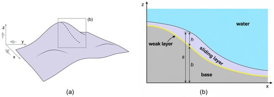
As shown in Figure 1, the three-dimensional conservation equations are normalised and integrated vertically from the weak layer surface to the seabed, where b and s denote the basal and seabed elevations, respectively, and h = s − b is the local sliding-layer thickness. The momentum balance is projected onto the basal normal. Higher-order terms are neglected, while the leading contributions from gravity, seismic inertia, and terrain curvature are retained. A detailed derivation can be found in Zhang et al. [37]. The resulting depth-averaged governing equations are

$${\displaystyle \frac{\partial h}{\partial t}}+{\displaystyle \frac{\partial h{u}_x}{\partial x}}+{\displaystyle \frac{\partial h{u}_y}{\partial y}}=0$$

(1)

$${\displaystyle \frac{\partial h{u}_x}{\partial t}}+{\displaystyle \frac{\partial h{u}_x^2}{\partial x}}+{\displaystyle \frac{\partial h{u}_x{u}_y}{\partial y}}={\displaystyle \frac{\partial h{\sigma }_{xx}}{\rho \partial x}}+{\displaystyle \frac{\partial h{\sigma }_{xy}}{\rho \partial y}}-{\displaystyle \frac{1}{2}}{C}_{\mathrm{f}}\xi ‖U‖u_x-\mu h{\displaystyle \frac{\partial b}{\partial x}}-{\displaystyle \frac{{\tau }_{w,x}}{\rho }}-a_{x}h$$

(2)

$${\displaystyle \frac{\partial h{u}_y}{\partial t}}+{\displaystyle \frac{\partial h{u}_x{u}_y}{\partial x}}+{\displaystyle \frac{\partial h{u}_y^2}{\partial y}}={\displaystyle \frac{\partial h{\sigma }_{yy}}{\rho \partial y}}+{\displaystyle \frac{\partial h{\sigma }_{xy}}{\rho \partial x}}-{\displaystyle \frac{1}{2}}{C}_{\mathrm{f}}\xi ‖U‖u_y-\mu h{\displaystyle \frac{\partial b}{\partial y}}-{\displaystyle \frac{{\tau }_{w,y}}{\rho }}-a_{y}h$$

(3)

where the parameter μ represents the combined effects of gravity, buoyancy, seismic loading, and centrifugal acceleration on the basal stress and is given by

$$\mu ={\displaystyle \frac{1}{{\varphi }^2}}\left[g\left(1-\xi \right)+a_z-{\displaystyle \frac{a_x\partial b}{\partial x}}-{\displaystyle \frac{a_y\partial b}{\partial y}}+v^{\mathrm{T}}Hv\right]$$

(4)

where t is time; x, y and z are the Cartesian coordinates; u_x, u_y and u_z are the depth-averaged velocity components, U = (u_x, u_y, u_z)^T; ρ and ρ′ are the total and submerged densities; ξ = 1 − ρ′/ρ is the density contrast; σ_xx, σ_yy and σ_xy are the depth-averaged in-plane stresses; τ_w,x and τ_w,y are the basal shear stress components; a_x, a_y and a_z are the seismic acceleration components in the east–west, north–south, and vertical directions, respectively; g denotes gravitational acceleration; v = (u_x, u_y)^T; H is the Hessian matrix of the basal surface; $\varphi =\sqrt{{\left({\displaystyle \frac{\partial b}{\partial x}}\right)}^2+{\left({\displaystyle \frac{\partial b}{\partial y}}\right)}^2+1}$ is the geometric factor. Resistance from the ambient water is represented by the skin friction coefficient C_f, given by

$$C_{\mathrm{f}}={\left(1.89+1.62\log {\displaystyle \frac{L_{\mathrm{f}}}{k_{\mathrm{f}}}}\right)}^{-2.5}$$

(5)

where L_f is the maximum slide length along the principal direction of movement and k_f is the characteristic surface-roughness length [53,54].

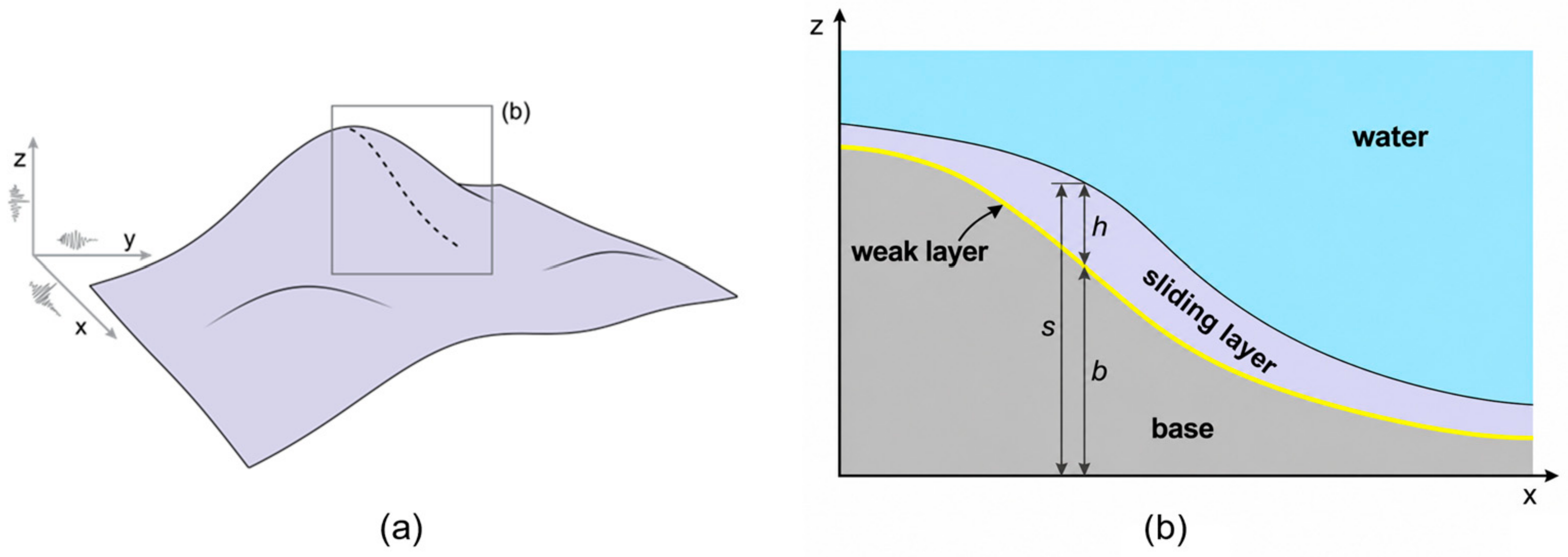
Figure 1. Schematic representation of a submarine landslide over three-dimensional terrain: (a) basal topography, with the box indicating the location of the cross-section in (b); (b) cross-section through the sliding and weak layers.

It is prescribed that soils of both layers exhibit linear strain softening. In the sliding layer, strength decreases with accumulated von Mises plastic strain, while rate dependence is represented by the Herschel–Bulkley relation

$${\tau }_{\mathrm{s}}={\tau }_{\mathrm{p},\mathrm{s}}\cdot \max \left[1+{\displaystyle \frac{1-S_{\mathrm{t},\mathrm{s}}}{S_{\mathrm{t},\mathrm{s}}}}\cdot {\displaystyle \frac{{\epsilon }_{\mathrm{s}}^{\mathrm{p}}}{{\epsilon }_{\mathrm{s},\mathrm{r}}^{\mathrm{p}}}},{\displaystyle \frac{1}{S_{\mathrm{t},\mathrm{s}}}}\right]\cdot \left[1+\eta {\left({\displaystyle \frac{\dot{\gamma }}{{\dot{\gamma }}_{\mathrm{ref}}}}\right)}^n\right]$$

(6)

where τ_s and τ_p,s are the mobilised shear strength and peak undrained shear strength of the sliding layer, respectively. ${\epsilon }_{\mathrm{s}}^{\mathrm{p}}$ is the accumulated von Mises plastic strain, and ${\epsilon }_{\mathrm{s},\mathrm{r}}^{\mathrm{p}}$ is its value at the remoulded strength. S_t,s is the soil sensitivity of the sliding layer. γ̇ and γ̇_ref are the shear strain rate and reference shear strain rate, respectively. η and n are the dimensionless viscous parameter and flow index, respectively. Before yielding, stress in the sliding layer is updated elastically using the shear modulus G_s. Simple shear is assumed in the weak layer, and its resistance decreases with accumulated plastic shear displacement. The direction of resistance is defined by U/‖U‖:

$${\tau }_{\mathrm{w}}={\tau }_{\mathrm{p},\mathrm{w}}\cdot \max \left[1+{\displaystyle \frac{1-S_{\mathrm{t},\mathrm{w}}}{S_{\mathrm{t},\mathrm{w}}}}\cdot {\displaystyle \frac{{\delta }^{\mathrm{p}}}{{\delta }_{\mathrm{r}}^{\mathrm{p}}}},{\displaystyle \frac{1}{S_{\mathrm{t},\mathrm{w}}}}\right]\cdot \left[1+\eta {\left({\displaystyle \frac{‖U‖}{v_{\mathrm{ref}}}}\right)}^n\right]\cdot {\displaystyle \frac{U}{‖U‖}}$$

(7)

where τ_w and τ_p,w are the weak layer shear stress vector and peak undrained shear strength, respectively. δ^p is the accumulated plastic shear displacement, and ${\delta }_{\mathrm{r}}^{\mathrm{p}}$ is its value at the remoulded strength. S_t,w is the soil sensitivity of the weak layer, and v_ref is the reference velocity. The analyses are performed in terms of total stress for soils under undrained conditions. The generation of excess pore pressure in the shear band is not modelled explicitly but is represented by strain softening, which is controlled by the soil sensitivity and the plastic displacement to the remoulded strength. Hydrodynamic uplift and hydroplaning are neglected, and the effect of the ambient water on the sliding mass is accounted for through buoyancy and skin friction drag.

The complete formulations and details of numerical implementation can be found in Zhang et al. [37], and are not repeated here.

2.2. Ashton Seamount Landslide: Geological Setting and Model Setup

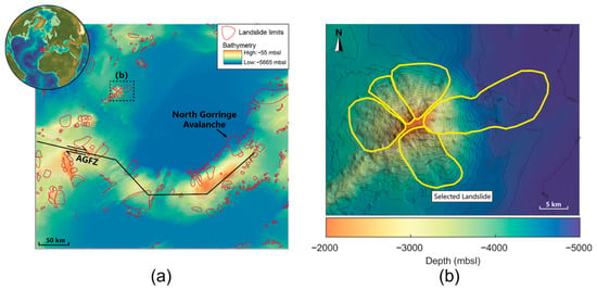
The Ashton Seamount landslide is located on the tectonically active southwest Iberian margin, close to the Azores–Gibraltar plate boundary. Landslide and turbidite deposits in the Gulf of Cádiz have been interpreted as records of off-fault palaeoseismicity [55,56,57,58,59,60]. The Marques de Pombal Slide and North Gorringe Avalanche have also been associated with active faulting and earthquake loading [61,62]. Ashton is selected here as its mapped scar is spatially distinct from those of neighbouring large landslides (Figure 2).

Figure 2. (a) Catalogued landslides (red outlines) on the southwest Iberian margin and surface trace of the Azores–Gibraltar Fracture Zone (AGFZ), with the dashed box indicating the area shown in (b); (b) detailed bathymetry of Ashton Seamount, showing the landslide limits (yellow outlines) and the landslide selected for analysis. The figure was prepared by the authors from the MAGICLAND database of Gamboa et al. [63] and the geological information in Merle et al. [64].

The current bathymetry and reconstructed pre-failure surface were obtained from the database of Gamboa et al. [63]. Site-specific geotechnical measurements are unavailable; the sediment density and coefficient governing the increase in undrained strength with depth are therefore based on borehole data from the southwest Iberian margin [65]. Weak layers exist at lithological boundaries, with undrained shear strength much lower than that of the adjacent overlying layer [17]. The Miocene–Pliocene/Pliocene–Quaternary boundary is accordingly adopted as the weak layer. Seismic profiles across the nearby North Gorringe Avalanche place this boundary 550–700 m below the seabed [62] (Figure 2a). The peak undrained strength of the weak layer is expressed as a fraction α of that in the adjacent sliding layer. Values of α = 0.8, 0.85, 0.9 and 0.95 are examined. The plastic shear displacement required to reach the remoulded strength is specified as 0.2 m, which is within the range of 0.1–0.5 m reported for clays [66], and a soil sensitivity of 2 is assigned to both layers. Based on the mapped landslide dimensions and the reported range of 0.01–0.1 m for the surface roughness of submarine sliding masses [53,54], L_f and k_f are set to 10 km and 0.1 m, respectively; Equation (5) then gives C_f = 0.0032. All inputs for the DAM analyses are listed in Table 1.

Table 1. Input parameters for the Ashton Seamount landslide.

Parameter	Value	Unit
Saturated density, ρ *	1796	kg/m3
Undrained shear strength increase coefficient with depth, ks *	0.35	–
Plastic shear displacement at remoulded strength, ${\delta }_{\mathrm{r}}^{\mathrm{p}}$	0.2	m
Plastic shear strain at remoulded strength, ${\epsilon }_{\mathrm{s},\mathrm{r}}^{\mathrm{p}}$	0.2	–
Soil sensitivity in the weak layer, St,w	2	–
Soil sensitivity in the sliding layer, St,s	2	–
Weak layer to sliding layer strength ratio, α	0.85	–
Depth-averaged peak undrained shear strength in sliding layer, τp,s	ksγ’h/2	kPa
Peak undrained shear strength in weak layer, τp,w	αksγ’h	kPa
Shear modulus in sliding layer, Gs	60	MPa
Shear stiffness in weak layer, Gw	165.6τp,w	kPa/m
Dimensionless viscous parameter, η	0.15	–
Flow index, n	0.15	–
Reference velocity, vref	1	m/s

* Data for submarine sediments on the southwest Iberian margin from Collico et al. [65].

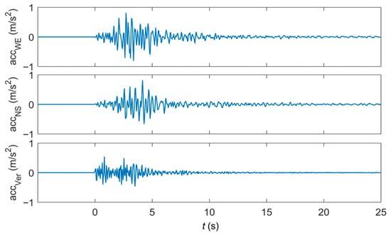
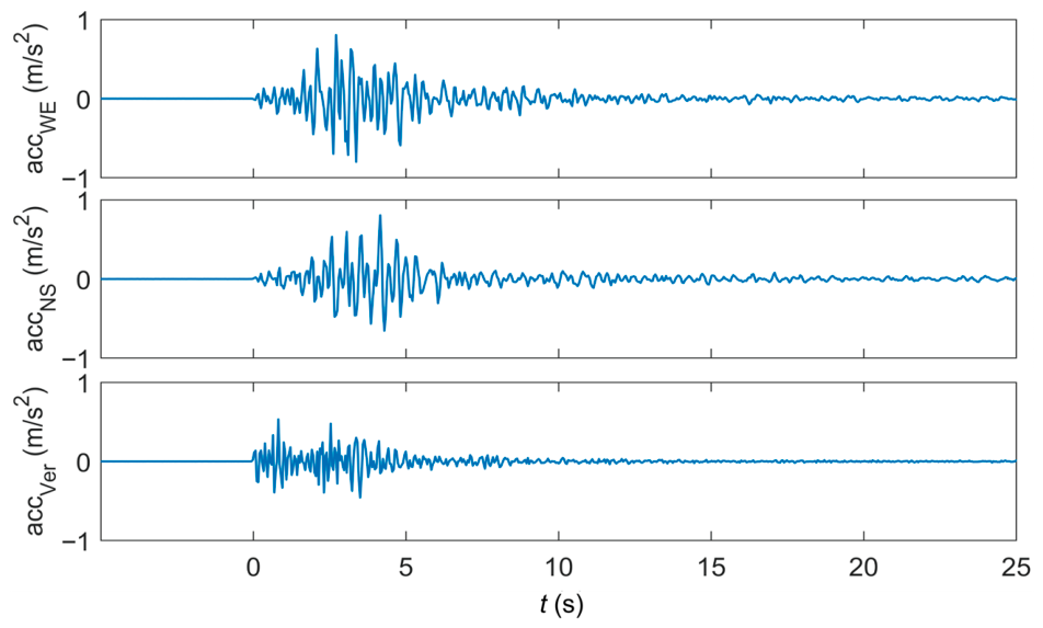
The acceleration records from an earthquake in 1998 at the nearest available station in the Azores (Event ID PT-1998-0020) are taken as the seismic input (Figure 3). The records were obtained from the Engineering Strong Motion Database [67]. The Azores and Ashton Seamount both lie along the Azores–Gibraltar Fracture Zone (Figure 2a). As no instrumental record exists for the earthquake that triggered the Ashton Seamount landslide, the records are used without scaling as a representative input, and the analysis should be regarded as a conditional back-analysis.

Figure 3. Three components of the input seismic acceleration.

The computational domain measures 46.4 × 60 km and comprises 2321 × 3001 cells. The final morphologies with grid sizes of 20 and 40 m are close to each other, suggesting that computational convergence is achieved when the grid size is no larger than 40 m. The grid size of 20 m is employed as a balance between computational accuracy and cost. In the DAM, the shear band is represented by the weak layer, and the softening of the weak layer is governed by the accumulated plastic shear displacement rather than strains. Essentially, the shear band thickness does not depend on the grid size. The propagation of the shear band was demonstrated and verified in the mesh sensitivity analysis by Zhang et al. [37]. The time step is determined by the stability criterion presented in Zhang et al. [37], Δt ≤ CΔx/√(E/ρ) with C = 0.8. The DAM is implemented in MATLAB R2023b (MathWorks, Natick, MA, USA). It takes 38 min to complete the simulation of the entire sliding process on a single NVIDIA GeForce RTX 4060 GPU (NVIDIA, Santa Clara, CA, USA).

2.3. South China Sea Canyon System: Model Setup

The study area is located on the northern continental slope of the South China Sea at water depths of approximately 230–1420 m. This region experiences canyon incision, with slope gradients ranging from approximately 20° to 40°. Branching gullies form multiple pathways down the slope. A representative canyon segment measuring 6.2 × 9.4 km is selected. The bathymetry is interpolated onto a 4 m computational grid containing 1551 × 2351 cells. The onset times and runouts corresponding to the grid sizes of 4, 5, 8, and 10 m are close to each other, with predicted peak velocities of 39–41 m/s. The final affected area decreases from 31.7 to 23.4 km² as the grid is refined; however, the difference in the affected areas between grid sizes of 5 and 4 m is only 4%. The grid size of 4 m is therefore adopted.

Soil strengths were derived from three cone penetration tests (CPTs) conducted in the study area, located on the upper slope near the shelf break, on the middle slope, and on the canyon floor at the foot of the slope. The sediment is composed of cohesive soils, and the undrained shear strength increased rapidly with depth in the upper 20 m and more gradually below this depth. The change in gradient was interpreted as the top of a weak layer [27]. The weak layer is thus identified by the change in the strength gradient rather than by a peak strength lower than that of the overlying sediment. Therefore, the soil at a depth of 20 m is taken as the weak layer. The peak undrained strength of the weak layer is taken as 100 kPa from the CPT measurements at 20 m depth. Based on the CPT data, the peak strength in the overlying 0–20 m sliding layer is taken to increase linearly with depth, giving a depth-averaged value of τ_p,s = 50 kPa. The saturated sediment density was measured as ρ = 1969 kg/m³. Repeated T-bar tests at Liwan 3-1 in the northern South China Sea indicate profile-scale soil sensitivities of approximately 5–9 [68]; S_t,w and S_t,s are therefore both taken as 5. The plastic shear displacement required to reach the remoulded strength is taken as ${\delta }_{\mathrm{r}}^{\mathrm{p}}$ = 0.20 m, within the range of 0.1–0.5 m reported for clays [66].

The sliding-layer shear modulus is specified as G_s = 7.57 MPa. As τ_p,s = 50 kPa, E/τ_p,s is taken as 453, and the ratio lies within the typical range of 300–800 for offshore clays [24]. The weak layer shear stiffness is taken as G_w = 16.56 MPa/m. For saturated marine soft clay from the Nansha area, Liu et al. [69] reported an exponential rate parameter of approximately 0.13. This rate dependence is reproduced between normalised strain rates of 1 and 10 using n = 0.15 and η = 0.47. For L_f = 5 km and k_f = 0.1 m, Equation (5) gives C_f = 0.0036. The inputs are listed in Table 2.

Table 2. Input parameters for the South China Sea canyon system.

Parameter	Value	Unit
Saturated density, ρ	1969	kg/m3
Peak undrained strength in weak layer, τp,w	100	kPa
Averaged peak undrained strength in sliding layer, τp,s	50	kPa
Soil sensitivity in the weak layer, St,w	5	–
Soil sensitivity in the sliding layer, St,s	5	–
Plastic shear displacement at remoulded strength, ${\delta }_{\mathrm{r}}^{\mathrm{p}}$	0.2	m
Plastic shear strain at remoulded strength, ${\epsilon }_{\mathrm{s},\mathrm{r}}^{\mathrm{p}}$	0.2	–
Shear modulus in sliding layer, Gs	7.57	MPa
Shear stiffness in weak layer, Gw	16.56	MPa/m
Dimensionless viscous parameter, η	0.47	–
Flow index, n	0.15	–
Reference velocity, vref	1	m/s
Skin friction coefficient, Cf	0.0036	–

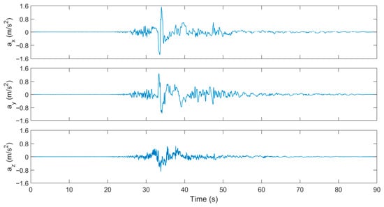
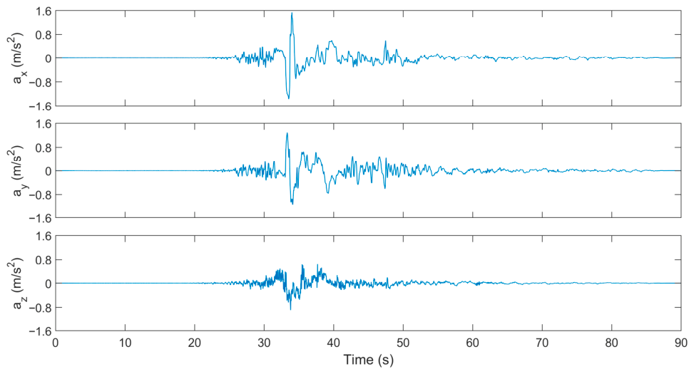
Three components of the 1999 Chi-Chi earthquake recorded at station TCU052 (M_w 7.3; PEER NGA-West2 record RSN 1492) are used as the seismic input [70], as the station is close to the northern South China Sea and has a similar tectonic setting. The horizontal peak ground acceleration for a 1000-year return period was 154 Gal, following a site-specific seismic hazard assessment of the study area, which is located close to the active slope fault zone of the northern South China Sea [71]. A common scale factor is applied to all three components, giving peak accelerations of 154, 128, and 89 Gal while preserving their relative amplitudes and phases (Figure 4). A unique record is used for each case, since this study aims to examine the robustness of the DAM to large-scale submarine landslides. The influence of different ground motions is to be explored in future work.

Figure 4. Three scaled acceleration components from the TCU052 record used as seismic input.

3. Results

3.1. Deep-Seated Ashton Seamount Landslide

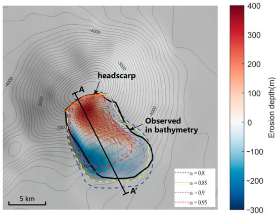
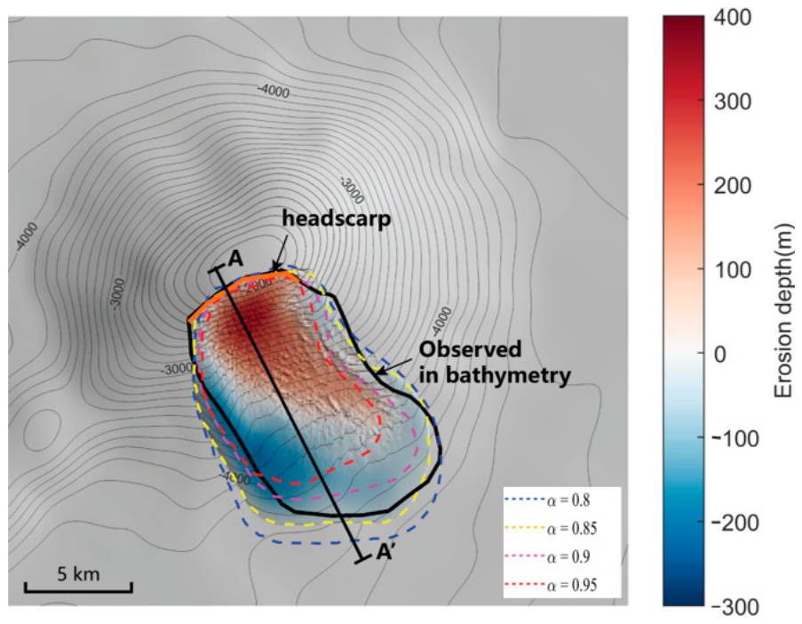
The predicted affected area decreases as α increases (Figure 5). For α = 0.8, the affected area exceeds the mapped downslope limit, while α = 0.9 and 0.95 suggest smaller affected areas. The numerical results with α = 0.85 are close to the mapped lateral and downslope margins, and α = 0.85 is therefore adopted in the analyses below. α is the only parameter calibrated, and the lateral and downslope margins of the mapped landslide are used.

Figure 5. Expansions of the landslides with various strength ratios of the weak layer.

3.1.1. Features of Shear Band Propagation and Sliding

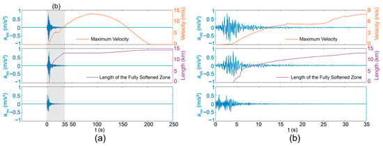
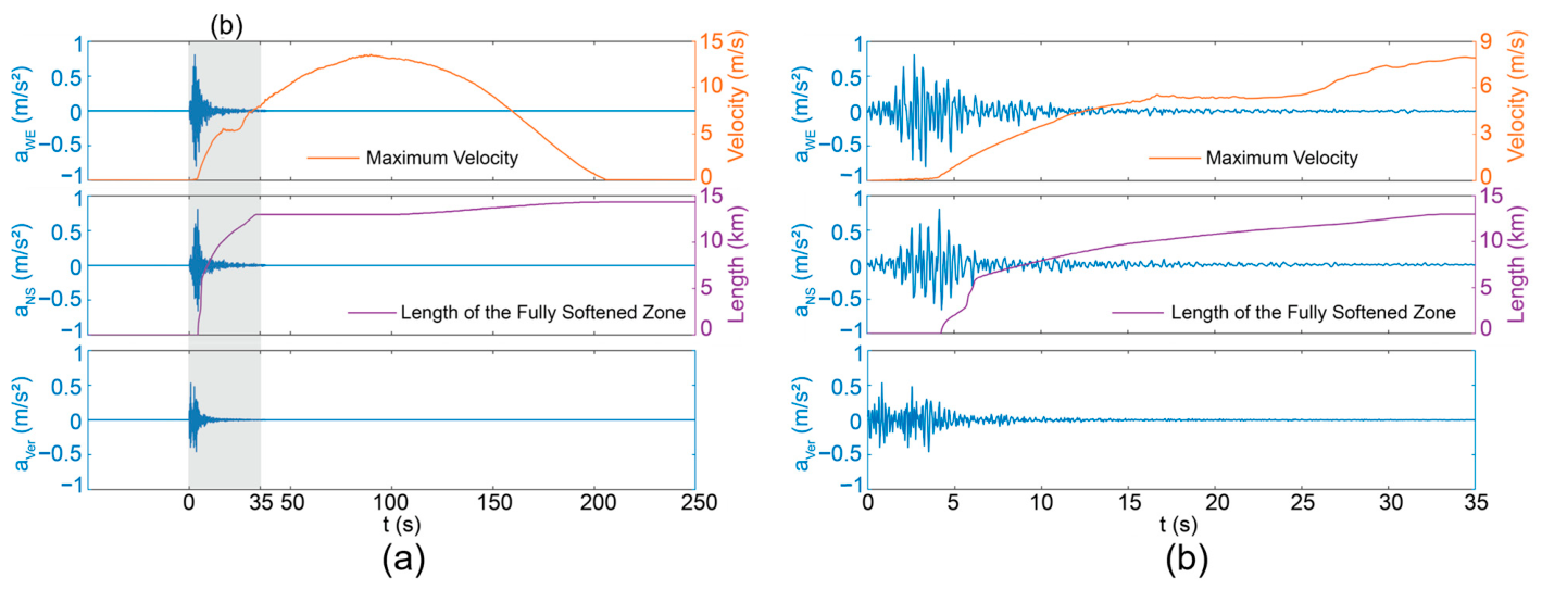
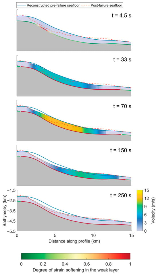
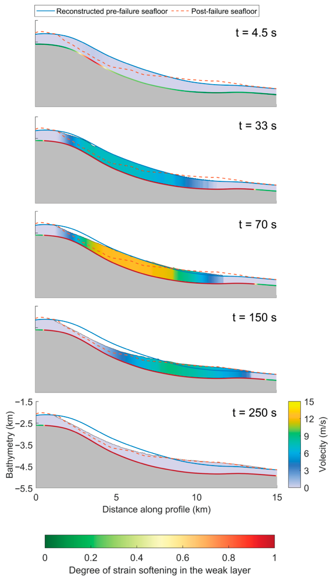
The slope failure and evolution of the slide are examined along a representative cross-section A–A′. The maximum sliding-layer velocity and growth of the fully softened zone in the weak layer are shown in Figure 6, while the corresponding sequence of initiation, propagation, slab failure, and runout is shown in Figure 7.

Figure 6. Seismic input and simulated response along cross-section A–A′: maximum velocity in the sliding layer and length of the fully softened zone in the weak layer during (a) the complete simulation, with the shaded band marking the period shown in (b), and (b) the seismic-triggering stage (0–35 s).

Figure 7. Simulated evolution of the Ashton Seamount landslide along cross-section A–A′.

The seismic input and the simulated response are compared in Figure 6. The fully softened zone appears at 4.3 s, where the horizontal accelerations reach their peak values. The fully softened zone then extends rapidly, reaching a length of 12.8 km by t = 33 s (Figure 6b). Its growth becomes very slow at the end of the earthquake, but is reactivated after 100 s, reaching a final length of 14.5 km. The maximum velocity of the sliding layer increases to ~5 m/s during the earthquake, peaks at 13.5 m/s at ~90 s, and falls to zero at ~205 s (Figure 6a).

At the onset of the earthquake, the shear stress induced by gravity and seismic acceleration increases in the weak layer. A fully softened zone is first formed at t = 4.3 s in the steepest part of the slope. Although the seismic acceleration decreases after t = 7 s, the weak layer has already softened and lost much of its resistance. By t = 33 s, the fully softened zone has extended to the slope toe downslope and to the slope crest upslope, and the propagation temporarily stops. The overlying sliding layer remains largely intact during the propagation and does not undergo slab failure until approximately t = 70 s. The failed mass accelerates downslope and further drives the fully softened zone to propagate again by t = 150 s. By t = 250 s, the sliding mass has become stationary, and the predicted post-failure morphology is consistent with the post-failure seafloor observed along section A–A′. This comparison is not used in the calibration.

At Ashton Seamount, the buried weak layer fails well before the thick overlying mass begins to move. This contrasts with the St. Niklausen case, where a 4.3 m thick slab failed almost immediately after its weak layer softened [37]. At Ashton, basal softening spreads across most of the slope within t = 33 s, yet the main slab does not move until around t = 70 s. This sequence indicates that in deep-seated landslides with a thick sliding layer, basal shear softening is a prerequisite for the detachment of the overlying slab.

3.1.2. Effect of Soil Sensitivity on the Slope Failure and Runout

Soil sensitivity, S_t, defined as the ratio of peak to remoulded undrained shear strength, dictates the magnitude of strength loss during softening. The baseline back-analysis in Section 3.1.1 uses S_t = 2 for both the weak and sliding layers, representing a lower-bound estimate for normally consolidated marine clay [13]. Given the wide variability in the soil sensitivity of marine clays, additional simulations are conducted with S_t,w = S_t,s = 3, 4, and 5. All other parameters remain unchanged.

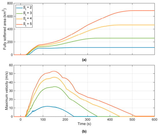
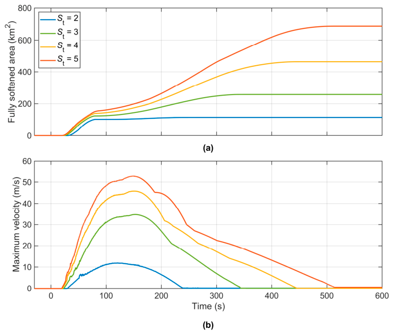
The fully softened area grows similarly in all four simulations during the first 80 s and reaches approximately 100–155 km² (Figure 8a). Initial softening is governed mainly by whether the combined gravitational and seismic shear stress exceeds the peak strength, showing little dependence on soil sensitivity. For S_t = 2, propagation ceases near 90 s, and the softened area stabilises at approximately 115 km². In contrast, cases with S_t = 3, 4 and 5 continue propagating, and the final softened area increases substantially with soil sensitivity.

Figure 8. Simulated response for different soil sensitivities: (a) fully softened area in the weak layer; (b) maximum velocity in the sliding layer.

The velocity histories exhibit a similar dependence on soil sensitivity (Figure 8b). The initial acceleration and timing of peak velocity are comparable among the four cases, whereas both the peak velocity and duration of movement increase with soil sensitivity. Landslide motion ceases at approximately 240 s for S_t = 2, compared with over 500 s for S_t = 5.

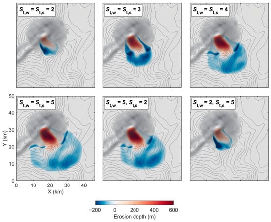
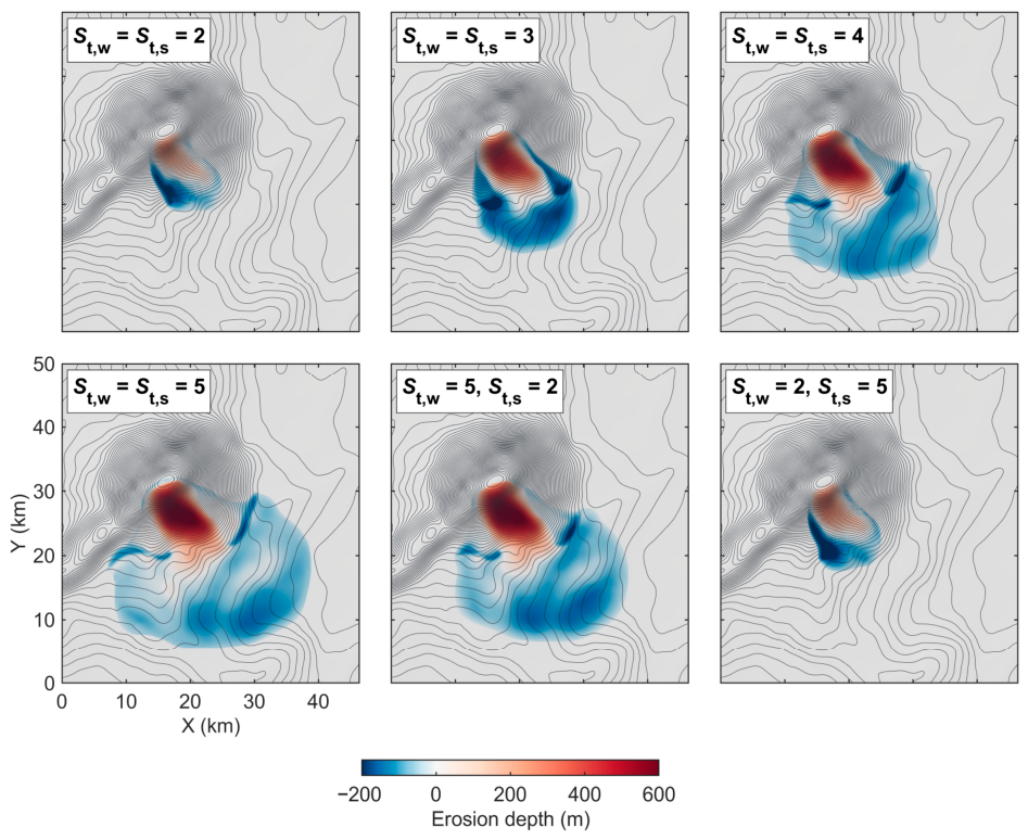
The effect of soil sensitivity on landslide runout and deposition is shown in Figure 9. As soil sensitivity increases, the deposit extends farther downslope and spreads more widely in the lateral direction, resulting in a thinner and more extensive deposit. The deposit remains within ~12 km from the headscarp at S_t = 2, while it extends ~24 km downslope and spreads over a width of ~26 km at S_t = 5 (Figure 9). The maximum erosion depth in the source area also increases from ~300 m to ~600 m. When S_t increases from 2 to 5, the peak velocity increases by more than four times, while the final affected area increases approximately six times. These results show that soil sensitivity strongly influences the predicted landslide mobility and final affected area.

Figure 9. Final morphologies at Ashton Seamount for different soil sensitivities of the weak and sliding layers.

To separate the contributions of the two layers, the soil sensitivities of the weak and sliding layers are also varied individually (Figure 9). With S_t,w = 5 and S_t,s = 2, an affected area of 583 km² is obtained, close to the 697 km² obtained when both soil sensitivities are 5. With S_t,w = 2 and S_t,s = 5, the affected area is 130 km², close to the 118 km² for S_t,w = S_t,s = 2. The final morphology is therefore governed mainly by the soil sensitivity of the weak layer. Initial yielding is governed by the peak strength, the slope geometry, and the seismic loading, whereas the subsequent propagation and mobility are controlled mainly by the soil sensitivity of the weak layer.

3.2. Earthquake-Triggered Landsliding in a Submarine Canyon System

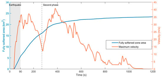
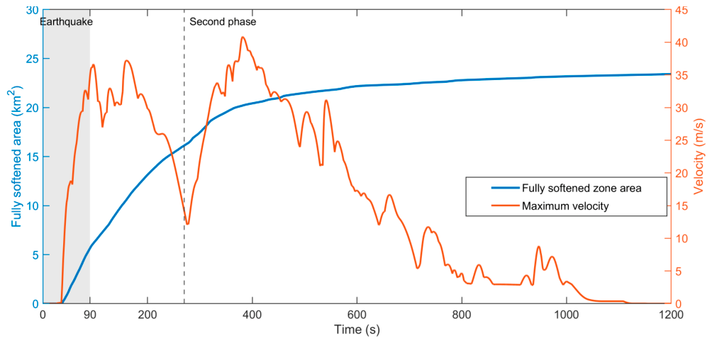
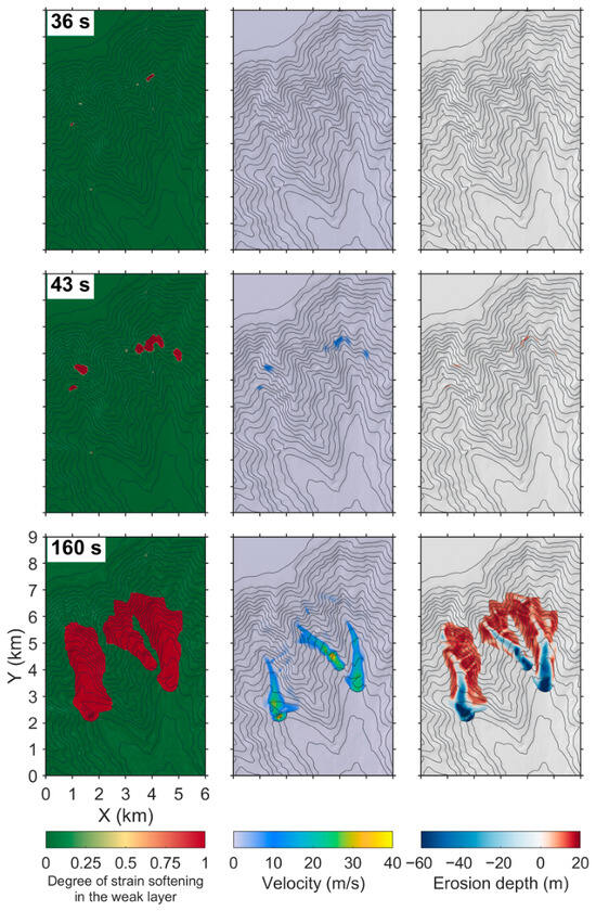
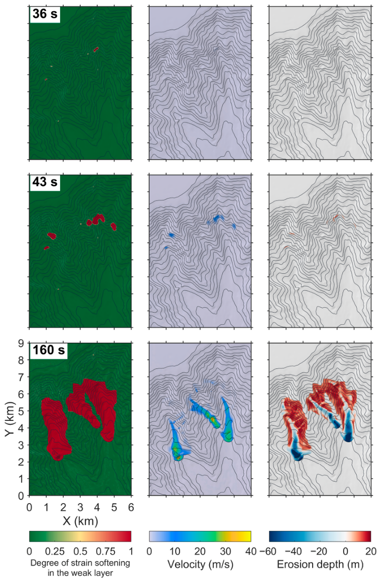
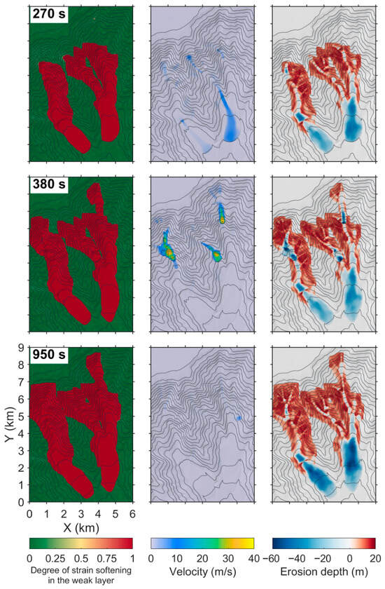
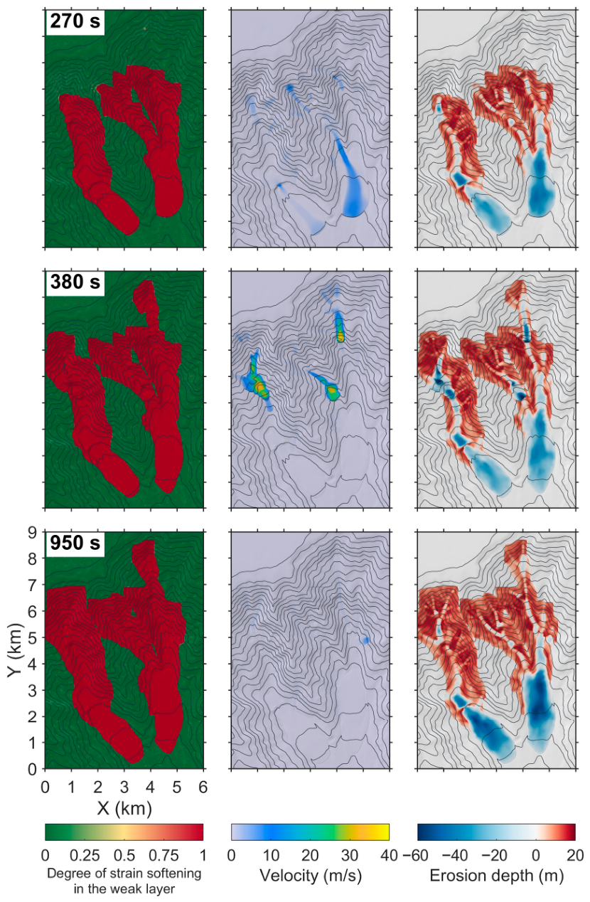
The fully softened area in the weak layer and maximum velocity in the sliding layer are shown in Figure 10. The failure process divides into two phases. The first phase covers co-seismic failure and movement driven by inertia and gravity until 270 s. The second phase begins at 270 s, 180 s after the end of the earthquake. The spatial evolution of the two phases is shown in Figure 11 and Figure 12, respectively.

Figure 10. Fully softened area in the weak layer and maximum velocity in the sliding layer. The grey band marks the duration of the earthquake and the dashed line the onset of the second phase.

Figure 11. Numerical evolution of the slides in the first phase, during and immediately after the earthquake.

Figure 12. Numerical evolution of the slides in the second phase, after the earthquake.

All three acceleration components reach their peak values at approximately 34 s (Figure 4). Shortly afterward, at 36 s, several zones with slope angles over 30° along the flanks of the canyon first become fully softened (Figure 11, 36 s). This spatial distribution demonstrates that failure is initiated locally where gravitational shear stress is high, rather than simultaneously across the canyon.

Between 36 and 42 s, the fully softened zones in the weak layer propagate and expand into five separate zones on the canyon flanks (Figure 11, 43 s). Broad deformation and rapid movement begin at 43 s. Softened zones expand as material moves downslope. Evacuation of sediment from the lower slopes removes lateral support for deposits on the upper slope. This loss of support promotes retrogressive failure. The earthquake ends at approximately 90 s, but the failed masses continue to move under gravity along several gullies. The flows follow separate canyon channels and merge locally where gullies converge. By 160 s, the sliding material has moved along three main gullies, forming erosion in the source areas and deposition at the flow fronts (Figure 11). In this first phase, a peak velocity of 37.2 m/s is reached at 160 s. The maximum velocity decreases to 14.17 m/s by 270 s due to energy dissipation and slope flattening, and the downslope source-to-deposit distance reaches approximately 6.4 km.

After 270 s, the fully softened zones expand along the upper and lateral boundaries of the disturbed areas, and mass movement resumes on the flanks of the canyon. At 270 s, motion has almost ceased except in the eastern gully (Figure 12, 270 s). By 380 s, three new fast-moving masses with velocities of 30–40 m/s have formed on the middle and upper slopes, and one more softened zone has extended upslope at the upper right of the domain (Figure 12). A new peak velocity of 40.8 m/s is recorded at 381 s. This second phase begins approximately 180 s after the earthquake has ended and is therefore not driven by ground acceleration. During the first phase, displacement of sediment alters slope geometry, removes lateral support for deposits on the upper slope, and forms new free faces. The resulting redistribution of stress brings sediment on the upper slope to a critical state, so the propagation of a shear band under gravity and retrogressive failure resume after the earthquake. By 1200 s, the total distance from source to deposit down the slope has reached 8.5 km, and the affected seabed area has expanded to 23.4 km². The deposits accumulate on the canyon floors in the lower part of the domain (Figure 12, 950 s).

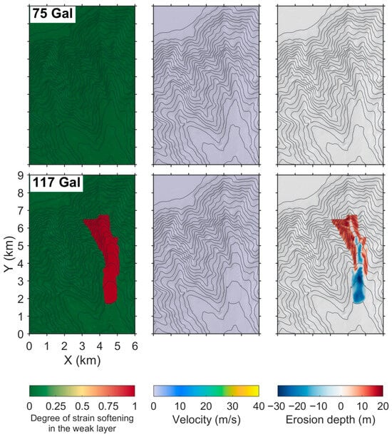
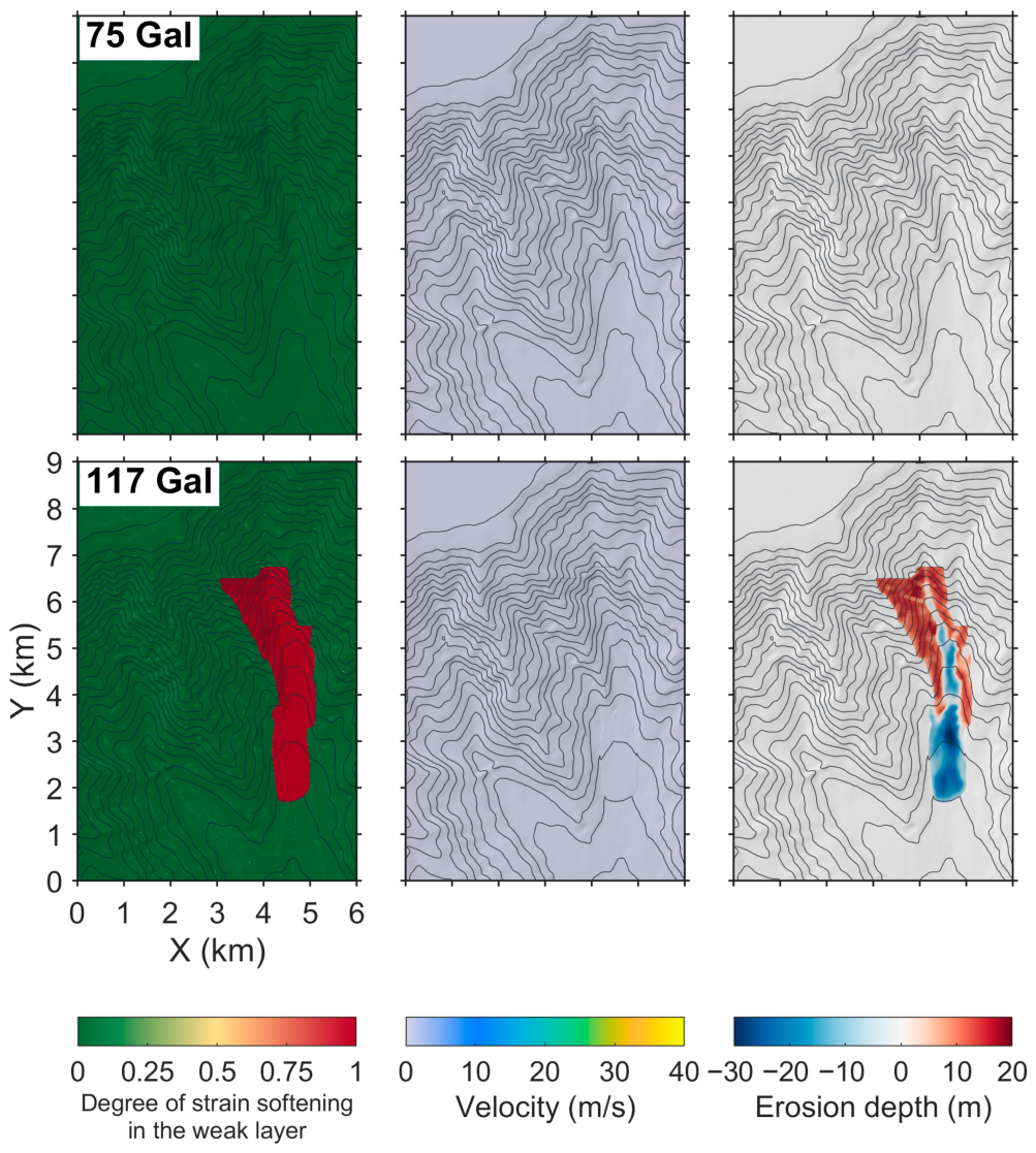
The influence of the earthquake intensity is examined by revisiting the case with the same record but scaled to the 200-year and 475-year levels of the site-specific assessment, i.e., horizontal peak ground accelerations of 75 and 117 Gal, respectively (Figure 13). No landslide is observed in the former. A single slope failure is triggered by the latter in the eastern gully, with a fully softened area of 4.8 km² and a peak velocity of 28.9 m/s. The movement stops at 380 s, and no further failure is triggered. It is worth noting again that the multiple failure sources, their merging along the gullies, and the post-seismic retrogression described above are predicted for the earthquake with the 1000-year return period. Under the horizontal peak ground acceleration of 117 Gal, sediment is evacuated from a single gully in the first phase. Under a horizontal peak ground acceleration of 154 Gal, sediment is evacuated from several gullies, and the lateral support of the upper slopes is removed, initiating renewed failures (Figure 12, 380 s). The renewed failure is therefore governed by the volume of sediment evacuated in the first phase.

Figure 13. Degree of strain softening, velocity and erosion depth at the end of the simulations under the 200-year (75 Gal) and 475-year (117 Gal) seismic levels.

4. Discussion

In previous assessments of earthquake-triggered submarine landslides, slope initiation and post-failure movement were mostly treated separately. Limit equilibrium, Newmark, and upper-bound analyses have been used to map seismically induced slope failures on lake slopes, continental margins, and canyon flanks [40,41,65,72], but the spreading of the failure and the travel of the failed mass cannot be described. Progressive failure along a weak layer is described by analytical SBP criteria, but only for idealised slope geometries [26,27,29]. The whole process can be simulated by large-deformation finite element and material point methods [16,33,34], but their three-dimensional applications have mostly been limited to individual slopes because of the computational cost. Earlier applications of DAMs with SBP were limited to idealised slopes and a small lake landslide [35,36,37]. In this study, the DAM is applied to natural bathymetry over domains of up to 46 × 60 km under three-component seismic loading, and the initiation, shear band propagation, slab failure, runout and post-seismic retrogression are simulated within one model. The simulation of the Ashton Seamount landslide is completed within 38 min on a single GPU, so such analyses are practical for parametric studies at the scale of a continental margin.

The analyses demonstrated have three main limitations. (a) Seismic accelerations are applied uniformly across each computational domain. Seismic wave propagation and ground motion amplification by local soft sediments and topography are therefore not accounted for. Local amplification on steep canyon flanks and at slope crests may cause earlier and more extensive strain softening than predicted, whereas attenuation would have the opposite effect. (b) The dynamics of the sliding mass are captured by the DAM, while hydroplaning underneath the slide and transformation of the failed mass into turbidity currents cannot be accounted for. These processes may lead to smaller basal resistance and transport of fine sediment further downslope. The runout and expansion of deposits may therefore be underestimated, particularly for the thin distal deposits. (c) Several soil properties, such as the soil sensitivity and strength of the weak layer, were not measured at Ashton Seamount, and the soil sensitivity in the South China Sea canyon is taken from a nearby site. At Ashton Seamount, the ratio of the affected area approaches six as soil sensitivity is increased from two to five, and the affected area decreases remarkably as the strength ratio of the weak layer is increased (Figure 5 and Figure 9).

The predicted footprints demonstrate the expansion of sediment failure and movements under the particular inputs, i.e., the landslide hazard [73]. Large submarine landslides may also result in tsunamis [74,75], but the present DAM does not calculate water-surface displacement, wave propagation, or coastal inundation.

5. Conclusions

The depth-averaged method (DAM) is used to investigate earthquake-triggered landslides in deep waters. Two typical scenarios are examined: a landslide with a weak layer buried deeply at Ashton Seamount and slope failures across a branching canyon system in the northern South China Sea. The main conclusions are summarised as follows:

(1) The evolution of submarine landslides with a deeply buried weak layer or large-scale mass movements is captured well by the DAM. At Ashton Seamount, with the weak layer strength ratio calibrated against the mapped footprint, the predicted head scarp and runout are consistent with the mapped landslide, which supports the applicability of the DAM to large landslides in deep waters.

(2) For the deep-seated landslide at Ashton Seamount, where the weak layer is inferred to be buried at a depth of 550–700 m, widespread basal softening is required prior to the catastrophic failure of the overlying mass. The influence of soil sensitivity on the initial softening process is insignificant, although it affects the sliding substantially. A large soil sensitivity suggests faster sliding and a larger affected area.

(3) Under the M_w 7.3 earthquake scenario, landslides in the South China Sea submarine canyon are initiated mainly on steep canyon flanks with slope angles greater than 30°. The resulting slide masses in various canyon channels reach a peak velocity of 40.8 m/s and an affected area of 23.4 km². Evacuation of sediment from the lower slopes impairs lateral support to the upper slopes during the earthquake. Subsequently, retrogressive failure and further sliding are triggered. The multiple failure sources and post-seismic propagation need to be accounted for in geohazard assessments; otherwise, the area of the potential hazard zone may be underestimated.

References

- Pope, E.L.; Talling, P.J.; Carter, L. Which earthquakes trigger damaging submarine mass movements: Insights from a global record of submarine cable breaks? Mar. Geol. 2017, 384, 131–146. [Google Scholar] [CrossRef] [Scilit]
- He, Z.; Okon, S.U.; Hu, P.; Zhang, H.; Ewa-Oboho, I.; Li, Q. Submarine gravity flows and their interaction with offshore pipelines: A review of recent advances. Eng. Geol. 2025, 347, 107914. [Google Scholar] [CrossRef] [Scilit]
- Du, P.; Li, L.; Kopf, A.; Wang, D.; Chen, K.; Shi, H.; Wang, W.; Pan, X.; Hu, G.; Zhang, P. Earthquake-induced submarine landslides (EQISLs) and a comparison with their terrestrial counterparts: Insights from a new database. Earth-Sci. Rev. 2025, 261, 105021. [Google Scholar] [CrossRef] [Scilit]
- Hampton, M.A.; Lee, H.J.; Locat, J. Submarine landslides. Rev. Geophys. 1996, 34, 33–59. [Google Scholar] [CrossRef] [Scilit]
- Masson, D.G.; Harbitz, C.B.; Wynn, R.B.; Pedersen, G.; Løvholt, F. Submarine landslides: Processes, triggers and hazard prediction. Philos. Trans. R. Soc. A Math. Phys. Eng. Sci. 2006, 364, 2009–2039. [Google Scholar] [CrossRef] [Scilit]
- Urlaub, M.; Talling, P.J.; Masson, D.G. Timing and frequency of large submarine landslides: Implications for understanding triggers and future geohazard. Quat. Sci. Rev. 2013, 72, 63–82. [Google Scholar] [CrossRef] [Scilit]
- Locat, J.; Lee, H.J. Submarine landslides: Advances and challenges. Can. Geotech. J. 2002, 39, 193–212. [Google Scholar] [CrossRef] [Scilit]
- Randolph, M.F.; Gaudin, C.; Gourvenec, S.M.; White, D.J.; Boylan, N.; Cassidy, M.J. Recent advances in offshore geotechnics for deep water oil and gas developments. Ocean Eng. 2011, 38, 818–834. [Google Scholar] [CrossRef] [Scilit]
- Forcellini, D.; Mina, D.; Karampour, H. The role of soil structure interaction in the fragility assessment of HP/HT unburied subsea pipelines. J. Mar. Sci. Eng. 2022, 10, 110. [Google Scholar] [CrossRef] [Scilit]
- Pan, H.; Li, C.; Li, H.; Ma, R.; Guo, J. Impact of local site conditions on seismic performance of free-spanning submarine pipelines: Underwater shaking table tests and numerical simulations. Earthq. Eng. Struct. Dyn. 2024, 53, 4223–4247. [Google Scholar] [CrossRef] [Scilit]
- Masson, D.G.; Wynn, R.B.; Talling, P.J. Large landslides on passive continental margins: Processes, hypotheses and outstanding questions. In Submarine Mass Movements and Their Consequences; Mosher, D.C., Shipp, R.C., Moscardelli, L., Chaytor, J.D., Baxter, C.D.P., Lee, H.J., Urgeles, R., Eds.; Springer: Dordrecht, The Netherlands, 2010; pp. 153–165. [Google Scholar]
- Talling, P.J.; Clare, M.; Urlaub, M.; Pope, E.; Hunt, J.E.; Watt, S.F.L. Large submarine landslides on continental slopes: Geohazards, methane release, and climate change. Oceanography 2014, 27, 32–45. [Google Scholar] [CrossRef] [Scilit]
- Randolph, M.F.; Gourvenec, S. Offshore Geotechnical Engineering; Spon Press: New York, NY, USA, 2011. [Google Scholar]
- Puzrin, A.M.; Germanovich, L.N.; Kim, S. Catastrophic failure of submerged slopes in normally consolidated sediments. Géotechnique 2004, 54, 631–643. [Google Scholar] [CrossRef]
- Viesca, R.C.; Rice, J.R. Nucleation of slip-weakening rupture instability in landslides by localised increase of pore pressure. J. Geophys. Res. Solid Earth 2012, 117, B03104. [Google Scholar] [CrossRef] [Scilit]
- Dey, R.; Hawlader, B.C.; Phillips, R.; Soga, K. Numerical modelling of submarine landslides with sensitive clay layers. Géotechnique 2016, 66, 454–468. [Google Scholar] [CrossRef] [Scilit]
- Gatter, R.; Clare, M.A.; Kuhlmann, J.; Huhn, K. Characterisation of weak layers, physical controls on their global distribution and their role in submarine landslide formation. Earth-Sci. Rev. 2021, 223, 103845. [Google Scholar] [CrossRef] [Scilit]
- Kvalstad, T.J.; Andresen, L.; Forsberg, C.F.; Berg, K.; Bryn, P.; Wangen, M. The Storegga Slide: Evaluation of triggering sources and slide mechanics. Mar. Pet. Geol. 2005, 22, 245–256. [Google Scholar] [CrossRef] [Scilit]
- L’Heureux, J.-S.; Longva, O.; Steiner, A.; Hansen, L.; Vardy, M.E.; Vanneste, M.; Brendryen, J.; Haflidason, H.; Kvalstad, T.J.; Forsberg, C.F.; et al. Identification of weak layers and their role for the stability of slopes at Finneidfjord, northern Norway. In Submarine Mass Movements and Their Consequences; Yamada, Y., Kawamura, K., Ikehara, K., Urgeles, R., Eds.; Advances in Natural and Technological Hazards Research 31; Springer: Dordrecht, The Netherlands, 2012; pp. 321–330. [Google Scholar]
- Quinn, P.E.; Diederichs, M.S.; Rowe, R.K.; Hutchinson, D.J. Development of progressive failure in sensitive clay slopes. Can. Geotech. J. 2012, 49, 782–795. [Google Scholar] [CrossRef] [Scilit]
- Puzrin, A.M.; Germanovich, L.N. The growth of shear bands in the catastrophic failure of soils. Proc. R. Soc. A Math. Phys. Eng. Sci. 2005, 461, 1199–1228. [Google Scholar] [CrossRef] [Scilit]
- Puzrin, A.M.; Saurer, E.; Germanovich, L.N. A dynamic solution of the shear band propagation in submerged landslides. Granul. Matter 2010, 12, 253–265. [Google Scholar] [CrossRef] [Scilit]
- Puzrin, A.M.; Germanovich, L.N.; Friedli, B. Shear band propagation analysis of submarine slope stability. Géotechnique 2016, 66, 188–201. [Google Scholar] [CrossRef] [Scilit]
- Zhu, Z.; Wang, D.; Zhang, W. Catastrophic submarine landslides with non-shallow shear band propagation. Comput. Geotech. 2023, 163, 105751. [Google Scholar] [CrossRef] [Scilit]
- Zhu, Z.; Wang, D.; Zhang, W. Submarine slope failure in sensitive clay due to buoyancy force of trapped gas. Comput. Geotech. 2025, 183, 107220. [Google Scholar] [CrossRef] [Scilit]
- Zhang, W.; Wang, D.; Randolph, M.F.; Puzrin, A.M. Catastrophic failure in planar landslides with a fully softened weak zone. Géotechnique 2015, 65, 755–769. [Google Scholar] [CrossRef] [Scilit]
- Zhang, W.; Wang, D.; Randolph, M.F.; Puzrin, A.M. From progressive to catastrophic failure in submarine landslides with curvilinear slope geometries. Géotechnique 2017, 67, 1104–1119. [Google Scholar] [CrossRef] [Scilit]
- Klein, B.; Leuch, C.; Puzrin, A.M. A GIS framework for prediction of basin-wide post-failure geometry of confined subaqueous landslides. Int. J. Numer. Anal. Methods Geomech. 2023, 47, 2405–2437. [Google Scholar] [CrossRef] [Scilit]
- Zhang, W.; Randolph, M.F.; Puzrin, A.M.; Wang, D. Criteria for planar shear band propagation in submarine landslides along weak layers. Landslides 2020, 17, 855–876. [Google Scholar] [CrossRef] [Scilit]
- Puzrin, A.M.; Gray, T.E.; Hill, A.J. Significance of the actual nonlinear slope geometry for catastrophic failure in submarine landslides. Proc. R. Soc. A Math. Phys. Eng. Sci. 2015, 471, 20140772. [Google Scholar] [CrossRef] [Scilit]
- Rushton, D.; Gray, T.; Puzrin, A.M.; Hill, A.J. GIS-based probabilistic slope stability assessment using shear band propagation. In Proceedings of the Offshore Technology Conference 2015, Houston, TX, USA, 4–7 May 2015; OTC-25871-MS, pp. 2537–2547. [Google Scholar]
- Sultan, N.; Garziglia, S. 3D stability analysis of submarine slopes: A probabilistic approach incorporating strain-softening behaviour. Landslides 2024, 21, 2695–2709. [Google Scholar] [CrossRef] [Scilit]
- Tran, Q.-A.; Rogstad, A.; Depina, I.; Fernández, F.; Alene, G.H.; Grimstad, G.; Nordal, S. 3D large deformation modeling of the 2020 Gjerdrum quick clay landslide. Can. Geotech. J. 2025, 62, 1–21. [Google Scholar] [CrossRef] [Scilit]
- Ceccato, F.; Yerro, A.; Di Carluccio, G. Simulating landslides with the material point method: Best practices, potentialities, and challenges. Eng. Geol. 2024, 338, 107614. [Google Scholar] [CrossRef] [Scilit]
- Zhang, W.; Puzrin, A.M. Depth integrated modelling of submarine landslide evolution. Landslides 2021, 18, 3063–3084. [Google Scholar] [CrossRef] [Scilit]
- Zhang, W.; Puzrin, A.M. How small slip surfaces evolve into large submarine landslides: Insight from 3D numerical modeling. J. Geophys. Res. Earth Surf. 2022, 127, e2022JF006640. [Google Scholar] [CrossRef] [Scilit]
- Zhang, R.; Wang, D.; Zhang, W. A depth-averaged method modeling three-dimensional submarine landslides caused by earthquakes. Comput. Geotech. 2026, 194, 108012. [Google Scholar] [CrossRef] [Scilit]
- Schnellmann, M.; Anselmetti, F.S.; Giardini, D.; McKenzie, J.A. Mass movement-induced fold-and-thrust belt structures in unconsolidated sediments in Lake Lucerne (Switzerland). Sedimentology 2005, 52, 271–289. [Google Scholar] [CrossRef] [Scilit]
- Schnellmann, M.; Anselmetti, F.S.; Giardini, D.; McKenzie, J.A. 15,000 years of mass-movement history in Lake Lucerne: Implications for seismic and tsunami hazards. Eclogae Geol. Helv. 2006, 99, 409–428. [Google Scholar] [CrossRef] [Scilit]
- Strasser, M.; Stegmann, S.; Bussmann, F.; Anselmetti, F.S.; Rick, B.; Kopf, A. Quantifying subaqueous slope stability during seismic shaking: Lake Lucerne as model for ocean margins. Mar. Geol. 2007, 240, 77–97. [Google Scholar] [CrossRef] [Scilit]
- Strasser, M.; Hilbe, M.; Anselmetti, F.S. Mapping basin-wide subaquatic slope failure susceptibility as a tool to assess regional seismic and tsunami hazards. Mar. Geophys. Res. 2011, 32, 331–347. [Google Scholar] [CrossRef] [Scilit]
- Canals, M.; Lastras, G.; Urgeles, R.; Casamor, J.L.; Mienert, J.; Cattaneo, A.; De Batist, M.; Haflidason, H.; Imbo, Y.; Laberg, J.S.; et al. Slope failure dynamics and impacts from seafloor and shallow sub-seafloor geophysical data: Case studies from the COSTA project. Mar. Geol. 2004, 213, 9–72. [Google Scholar] [CrossRef] [Scilit]
- Lee, H.J. Timing of occurrence of large submarine landslides on the Atlantic Ocean margin. Mar. Geol. 2009, 264, 53–64. [Google Scholar] [CrossRef] [Scilit]
- Twichell, D.C.; Chaytor, J.D.; Ten Brink, U.S.; Buczkowski, B. Morphology of late Quaternary submarine landslides along the US Atlantic continental margin. Mar. Geol. 2009, 264, 4–15. [Google Scholar] [CrossRef] [Scilit]
- Bryn, P.; Berg, K.; Forsberg, C.F.; Solheim, A.; Kvalstad, T.J. Explaining the Storegga Slide. Mar. Pet. Geol. 2005, 22, 11–19. [Google Scholar] [CrossRef] [Scilit]
- Vanneste, M.; Mienert, J.; Bünz, S. The Hinlopen Slide: A giant, submarine slope failure on the northern Svalbard margin, Arctic Ocean. Earth Planet. Sci. Lett. 2006, 245, 373–388. [Google Scholar] [CrossRef] [Scilit]
- Joanne, C.; Collot, J.-Y.; Lamarche, G.; Migeon, S. Continental slope reconstruction after a giant mass failure, the example of the Matakaoa Margin, New Zealand. Mar. Geol. 2010, 268, 67–84. [Google Scholar] [CrossRef] [Scilit]
- Green, A.N.; Uken, R. Submarine landsliding and canyon evolution on the northern KwaZulu-Natal continental shelf, South Africa, SW Indian Ocean. Mar. Geol. 2008, 254, 152–170. [Google Scholar] [CrossRef] [Scilit]
- He, Y.; Zhong, G.; Wang, L.; Kuang, Z. Characteristics and occurrence of submarine canyon-associated landslides in the middle of the northern continental slope, South China Sea. Mar. Pet. Geol. 2014, 57, 546–560. [Google Scholar] [CrossRef] [Scilit]
- Dennielou, B.; Guambe, I.H.; Matsena, C.P.; Mugabe, J.A.; Achimo, M.; Jouet, G. Insight into contrasting patterns of sedimentation from shelf edge to base-of-slope on the Mozambique–Zambezi margin (17°30′ S–20° S) during the last 40 ka. Mar. Geol. 2022, 451, 106886. [Google Scholar] [CrossRef] [Scilit]
- Greene, H.G.; Maher, N.M.; Paull, C.K. Physiography of the Monterey Bay National Marine Sanctuary and implications about continental margin development. Mar. Geol. 2002, 181, 55–82. [Google Scholar] [CrossRef] [Scilit]
- Smith, D.P.; Kvitek, R.; Iampietro, P.J.; Wong, K. Twenty-nine months of geomorphic change in upper Monterey Canyon (2002–2005). Mar. Geol. 2007, 236, 79–94. [Google Scholar] [CrossRef] [Scilit]
- Norem, H.; Locat, J.; Schieldrop, B. An approach to the physics and the modeling of submarine flowslides. Mar. Geotechnol. 1990, 9, 93–111. [Google Scholar] [CrossRef] [Scilit]
- Elverhøi, A.; Breien, H.; De Blasio, F.V.; Harbitz, C.B.; Pagliardi, M. Submarine landslides and the importance of the initial sediment composition for run-out length and final deposit. Ocean Dyn. 2010, 60, 1027–1046. [Google Scholar] [CrossRef] [Scilit]
- Garcia-Orellana, J.; Gràcia, E.; Vizcaino, A.; Masqué, P.; Olid, C.; Martínez-Ruiz, F.; Piñero, E.; Sanchez-Cabeza, J.-A.; Dañobeitia, J. Identifying instrumental and historical earthquake records in the southwest Iberian margin using 210Pb turbidite chronology. Geophys. Res. Lett. 2006, 33, L24601. [Google Scholar] [CrossRef] [Scilit]
- Terrinha, P.; Matias, L.; Vicente, J.; Duarte, J.; Luís, J.; Pinheiro, L.; Lourenço, N.; Diez, S.; Rosas, F.; Magalhães, V.; et al. Morphotectonics and strain partitioning at the Iberia–Africa plate boundary from multibeam and seismic reflection data. Mar. Geol. 2009, 267, 156–174. [Google Scholar] [CrossRef] [Scilit]
- Zitellini, N.; Gràcia, E.; Matias, L.; Terrinha, P.; Abreu, M.A.; DeAlteriis, G.; Henriet, J.P.; Dañobeitia, J.J.; Masson, D.G.; Mulder, T.; et al. The quest for the Africa–Eurasia plate boundary west of the Strait of Gibraltar. Earth Planet. Sci. Lett. 2009, 280, 13–50. [Google Scholar] [CrossRef] [Scilit]
- Masson, D.G.; Arzola, R.G.; Wynn, R.B.; Hunt, J.E.; Weaver, P.P.E. Seismic triggering of landslides and turbidity currents offshore Portugal. Geochem. Geophys. Geosystems 2011, 12, Q12011. [Google Scholar] [CrossRef] [Scilit]
- Bartolome, R.; Gràcia, E.; Stich, D.; Martínez-Loriente, S.; Klaeschen, D.; de Lis Mancilla, F.; Lo Iacono, C.; Dañobeitia, J.J.; Zitellini, N. Evidence for active strike-slip faulting along the Eurasia–Africa convergence zone: Implications for seismic hazard in the southwest Iberian margin. Geology 2012, 40, 495–498. [Google Scholar] [CrossRef] [Scilit]
- Duarte, D.; Roque, C.; Ng, Z.L.; Hernández-Molina, F.J.; Magalhães, V.H.; Silva, S.M.; Llave, E. Structural control and tectono-sedimentary evolution of the Gulf of Cadiz, southwest Iberia since the late Miocene: Implications for the contourite depositional system. Mar. Geol. 2022, 449, 106818. [Google Scholar] [CrossRef] [Scilit]
- Minning, M.; Hebbeln, D.; Hensen, C.; Kopf, A. Geotechnical and geochemical investigations of the Marquês de Pombal landslide at the Portuguese continental margin. Nor. J. Geol. 2006, 86, 187–198. [Google Scholar]
- Lo Iacono, C.; Gràcia, E.; Zaniboni, F.; Pagnoni, G.; Tinti, S.; Bartolome, R.; Masson, D.G.; Wynn, R.B.; Lourenço, N.; Pinto de Abreu, M.; et al. Large, deepwater slope failures: Implications for landslide-generated tsunamis. Geology 2012, 40, 931–934. [Google Scholar] [CrossRef] [Scilit]
- Gamboa, D.; Omira, R.; Terrinha, P. A database of submarine landslides offshore west and southwest Iberia. Sci. Data 2021, 8, 185. [Google Scholar] [CrossRef] [Scilit]
- Merle, R.; Jourdan, F.; Marzoli, A.; Renne, P.R.; Grange, M.; Girardeau, J. Evidence of multi-phase Cretaceous to Quaternary alkaline magmatism on Tore–Madeira Rise and neighbouring seamounts from 40Ar/39Ar ages. J. Geol. Soc. 2009, 166, 879–894. [Google Scholar] [CrossRef] [Scilit]
- Collico, S.; Arroyo Alvarez de Toledo, M.; Urgelés Esclasans, R.; Gràcia Mont, E.; Devincenzi, M.J.; Pérez García, N. Probabilistic mapping of earthquake-induced submarine landslide susceptibility in the southwest Iberian margin. Mar. Geol. 2020, 429, 106296. [Google Scholar] [CrossRef] [Scilit]
- Skempton, A.W. Residual strength of clays in landslides, folded strata and the laboratory. Géotechnique 1985, 35, 3–18. [Google Scholar] [CrossRef] [Scilit]
- Luzi, L.; Lanzano, G.; Felicetta, C.; D’Amico, M.C.; Russo, E.; Sgobba, S.; Pacor, F. ORFEUS Working Group 5, 2020. Engineering Strong Motion Database (ESM), Version 2.0; Istituto Nazionale di Geofisica e Vulcanologia: Rome, Italy.
- Palix, E.; Wu, H.; Chan, N.; Zhou, Y. Liwan 3-1: How deepwater sediments from South China Sea compare with Gulf of Guinea sediments. In Proceedings of the Offshore Technology Conference, Houston, TX, USA, 6–9 May 2013; p. OTC-24010-MS. [Google Scholar]
- Liu, Y.; Luo, L.; Zhang, Y.; Lai, M.; Fu, Y. Triaxial experimental study on strength characteristics of saturated soft soil under different shear strain rates. In Proceedings of Conference on Sustainable Traffic and Transportation Engineering in 2023 (CSTTE 2023); Bieliatynskyi, A., Komyshev, D., Zhao, W., Eds.; Lecture Notes in Civil Engineering 603; Springer: Singapore, 2024; pp. 153–167. [Google Scholar]
- Ancheta, T.D.; Darragh, R.B.; Stewart, J.P.; Seyhan, E.; Silva, W.J.; Chiou, B.S.-J.; Wooddell, K.E.; Graves, R.W.; Kottke, A.R.; Boore, D.M.; et al. NGA-West2 database. Earthq. Spectra 2014, 30, 989–1005. [Google Scholar] [CrossRef] [Scilit]
- Lv, L.; Li, Z.; Wang, D.; Wang, W.; Dai, X.; Zeng, F.; Li, L.; Liang, H.; Hui, G.; Long, W.; et al. The latest activity of the slope fault zone (Pearl River Mouth) in northern South China Sea and implications for earthquake hazard assessments. Mar. Pet. Geol. 2024, 166, 106937. [Google Scholar] [CrossRef] [Scilit]
- Sultan, N.; Gaudin, M.; Berné, S.; Canals, M.; Urgeles, R.; Lafuerza, S. Analysis of slope failures in submarine canyon heads: An example from the Gulf of Lions. J. Geophys. Res. Earth Surf. 2007, 112, F01009. [Google Scholar] [CrossRef] [Scilit]
- Archetti, R.; Lamberti, A. Assessment of risk due to debris flow events. Nat. Hazards Rev. 2003, 4, 115–125. [Google Scholar] [CrossRef] [Scilit]
- Samaras, A.; Karambas, T.; Archetti, R. Simulation of tsunami generation, propagation and coastal inundation in the Eastern Mediterranean. Ocean Sci. 2015, 11, 643–655. [Google Scholar] [CrossRef] [Scilit]
- Masina, M.; Archetti, R.; Lamberti, A. 21 May 2003 Boumerdès earthquake: Numerical investigations of the rupture mechanism effects on the induced tsunami and its impact in harbors. J. Mar. Sci. Eng. 2020, 8, 933. [Google Scholar] [CrossRef] [Scilit]
Disclaimer/Publisher’s Note: The statements, opinions and data contained in all publications are solely those of the individual author(s) and contributor(s) and not of MDPI and/or the editor(s). MDPI and/or the editor(s) disclaim responsibility for any injury to people or property resulting from any ideas, methods, instructions or products referred to in the content. |
© 2026 by the authors. Licensee MDPI, Basel, Switzerland. This article is an open access article distributed under the terms and conditions of the Creative Commons Attribution (CC BY) license.