


Abstract
Protecting and restoring marine coastal ecosystems is essential to achieving Net Zero targets and counteracting biodiversity loss. Seagrass meadows are particularly important marine nature-based solutions due to their ability to store carbon, support biodiversity, and protect coastlines from extreme weather events. In the UK, however, Zostera marina (eelgrass) has experienced significant decline. While coastal restoration projects have increased considerably in recent years, their success relies on precise, site-specific assessments to be effective. Regional assessments of Z. marina habitat suitability remain challenging due to insufficient high-resolution environmental datasets that capture comprehensive habitat and environmental heterogeneity. For restoration purposes, model transferability allows the identification of areas where the absence of surveys has led to a lack of species presence data, yet they could potentially be suitable for restoration. To address this gap, we used machine-learning and classical statistical algorithms to forecast distribution of Z. marina across the United Kingdom (UK) and Ireland (Ire) and within six case study sites that span diverse coastal topographies and environmental conditions, enabling assessment of model predictions at different scales. Our results show bathymetry and photosynthetically active radiation (PAR)—both depth-related predictors—as the most important factors determining eelgrass occurrences. This has been shown to differ where high-resolution wave energy data is available, which has been shown to be a much more effective predictor. Despite all models performing well within their respective spatial domains, model transferability was limited. The large-scale model represented by the UK and Ireland showed better transferability to smaller local sites than the reverse, likely because it encompassed broader environmental gradients. In contrast, local models, calibrated over narrower environmental ranges, were less generalizable to wider regions. The broad-scale model tended to overpredict habitat suitability in shallow coastal areas, whereas the local-scale models offered more realistic predictions. These findings highlight that while large-scale models are valuable for identifying general patterns, local-scale models are more reliable for guiding site-specific restoration and conservation efforts in the UK and Ireland.
1. Introduction
Achieving and promoting nature recovery demand urgent action to protect and restore marine coastal ecosystems [1,2,3]. Among these, seagrass meadows play a crucial role as marine nature-based solutions, capturing and storing substantial amounts of carbon in their biomass and sediments while enhancing biodiversity and protecting coastlines from extreme weather events [3,4]. Despite their importance, seagrass meadows have declined sharply over the past century worldwide due to anthropogenic pressures such as nutrient pollution, coastal development, and physical disturbance like anchoring [5]. In this context, restoration of coastal habitats around the UK has rapidly grown in recent years, particularly for native oyster reefs, seagrass meadows and saltmarshes [6,7,8,9,10]. Once widespread across the UK, the subtidal, meadow-forming seagrass Zostera marina, eelgrass, has experienced significant decline, with around 44% of its cover lost since 1936 and historical evidence suggesting total losses may exceed 90% [11]. In some areas, improvements to water quality have led to a recovery of seagrass meadows [12], but the natural capacity of these plants to recolonise is considered to be low or slow [13]. Therefore, in areas where seagrass has significantly declined, has been lost altogether, or where distance to donor beds is not conducive to natural recovery, restoration is likely the only viable route of action to aid recovery but to also take advantage of this potential.
Global models estimating the extent, biomass, and biodiversity of seagrass ecosystems under current and future climate scenarios [14,15,16,17] have provided valuable baselines for ecosystem assessment and conservation planning. These estimates were performed using species distribution modelling (SDM), also known as habitat suitability modelling (HSM), a widely used approach across spatial and temporal scales [18,19,20,21,22,23]. The general lack of systematic biological surveys means it is impossible to be able to account for all individuals of a species all the time, which makes SDM invaluable in trying to fill these gaps [24]. However, the effectiveness of these models in local settings is often hindered by insufficient high-resolution environmental data, which are vital for capturing detailed habitat heterogeneity and for accurately targeting and prioritising localised restoration actions [25]. To meet these goals effectively, it is essential to develop fine-scale frameworks that evaluate the suitability of coastal environments for eelgrass recovery. This includes understanding how environmental variables influence Z. marina distribution and how well predictive models can be applied across spatial and geographic scales and transferred to unsampled locations. Since the strength and direction of ecological relationships often vary geographically [26], models built for national scale may not perform consistently elsewhere. Testing model generality therefore becomes crucial, not only for guiding restoration within a particular area but also for supporting broader approaches to seagrass recovery across the UK and beyond. Checking for model transferability can also be seen as a test of model generality or be used for model validation [27,28,29]. Fundamentally, SDMs are predictive models, rather than being designed for causal inference, which underlies the problems of transferability across space and scale [30,31,32]. If models have been overfitted and are too specific to local conditions, this transferability is reduced and then they become less useful in ecological terms [33].
The restoration of Z. marina meadows will have a number of ecological benefits as they support a wide range of ecosystem services such as providing shelter, direct and indirect sources of food, stabilisation of sediments and carbon storage [34]. Using SDM will help to inform the most suitable areas where seagrasses would be able to grow based upon thresholds of site-specific environmental conditions, allowing restoration efforts to be more targeted and cost-effective [35]. In this study, we (1) compare how environmental conditions influence seagrass presence between sites (i.e., local heterogeneity), (2) assess the transferability of HSMs across different spatial scales, and (3) evaluate how well HSMs trained in one geographic location perform when applied to other locations (spatial transference). We hypothesise that models produced for smaller spatial scales will not transfer well to larger spatial scales.
2. Methods
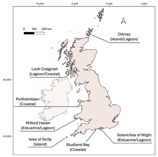
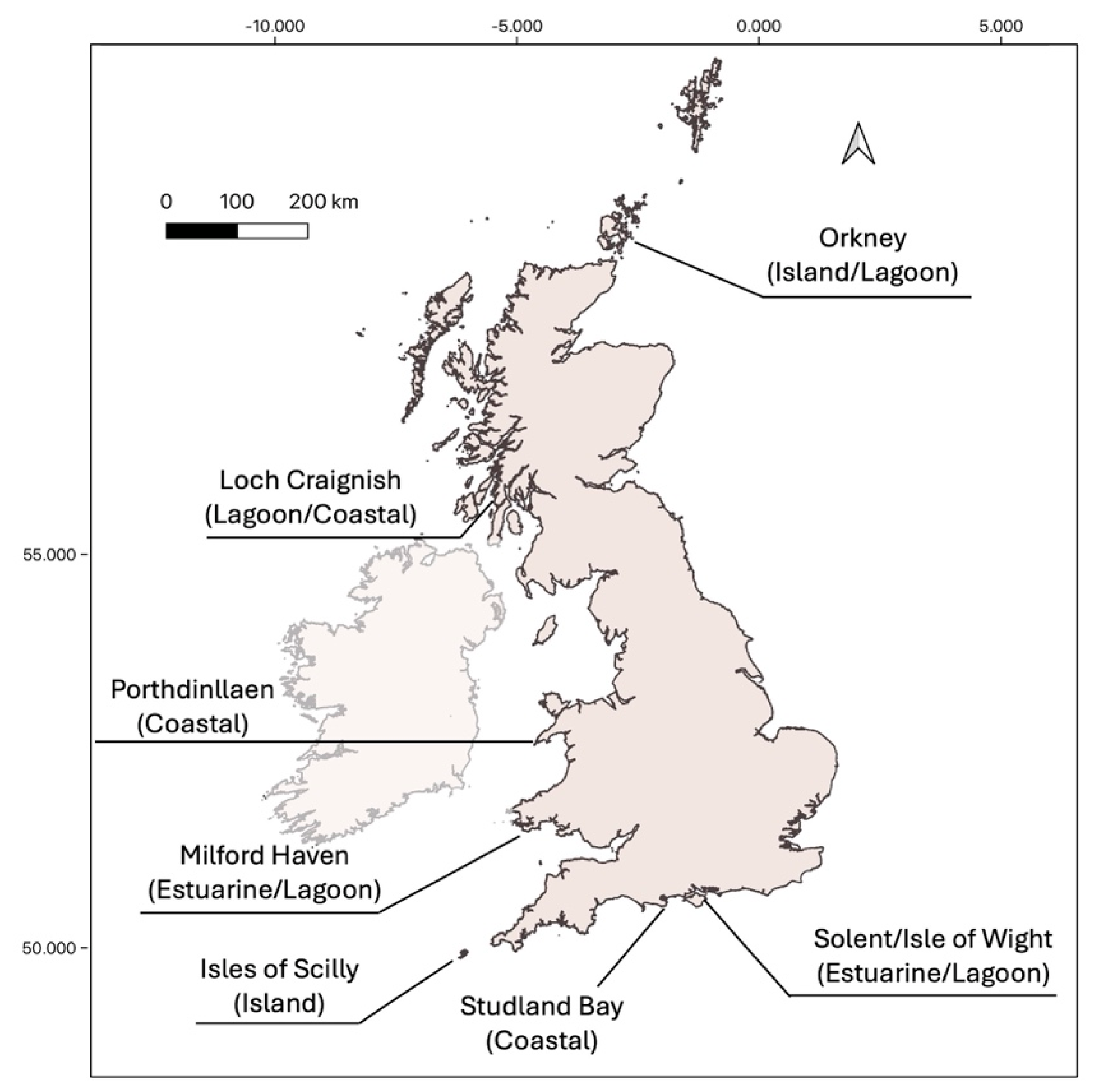
Six case study sites were selected to represent the range of coastal topography and environmental conditions in which seagrass meadows are found to typify seagrass sites around the UK (Table 1). These areas were also known to include existing seagrass meadows to enable HSM to be carried out at the case study site scale, but were chosen as part of a wider project to assess seagrass restoration for ocean wealth [36]. The sites (Figure 1) include estuaries, lagoons, coastal and island populations of seagrass, from relatively pristine (Isles of Scilly) to more turbid and disturbed (Milford Haven) conditions to encompass the range of conditions in which Z. marina can be found. Presence data included intertidal and subtidal seagrass meadows, although the majority of Z. marina is found subtidally around the British Isles.
Table 1.
Sites used for study with brief description of location and area in km2 utilised for HSM.
Figure 1.
Case study sites around the UK chosen to encompass environmental gradients and locations in which seagrass is found and, in some cases, already being restored. The larger-scale UK and Ireland model encompassed the whole coast of the UK and Ireland.
2.1. Site Descriptions
All sites used for modelling suitability of eelgrass are described in Table 1.
2.2. Occurrence Records
Seagrass presence data for the British Isles encompassing the case study sites were gathered using the most up-to-date sources utilised in previous studies ([37], Table S1). Data points were curated to thin out clustering (using the thinning tool in QGIS, minimum distance of 50 m between points) and to remove duplicates and anomalies (e.g., data points on land or far offshore). The presence data was then applied per case study site. Variable values were attained for all presence data and plotted to assess data distribution. Data that were significantly skewed were log-transformed as raster layers using QGIS before being integrated into the HSMs.
2.3. Environmental Predictors
Climate data for the modelling were sourced from the Copernicus Marine Environment Monitoring Service (CMEMS) and European Marine Observation and Data Network (EMODnet), comprising eight predictor variables spanning from 2001 to 2022 (Table S2).
Other important variables identified by Bertelli et al. [21] were not included in the models due to lack of availability or insufficient spatial resolution to capture the habitat of local study sites. Temporal resolution for temperature and salinity that were available from Copernicus allowed the monthly averaged data to be chosen based upon seasons that are significant for the life cycle of Z. marina. These months were: January as a potential for highest impacts due to wave action and wind speeds, March when seed germination and seedling emergence take place, August for peak biomass and seed production, and October for seed establishment and, as such, the suitable planting season for restoration work [38,39,40]. Salinity and temperature data from Copernicus were obtained for each of these months as an average of the daily means. Other data were not temporally resolved, so they remained as a single data layer (bathymetry, PAR, slope and currents). All environmental data layers were clipped to the areas of interest and resampled to the same resolution as the wave height and bathymetry data using the ‘resample’ function and the nearest neighbour method (‘ngb’) in the ‘raster’ package in R. As marine variable data often lacks coverage in shallow coastal zones, pixels covering both land and sea are often excluded [41]. To overcome this, a buffering tool was used in QGIS (raster ‘fill nodata’ tool) to interpolate data from neighbouring pixels to cover coastal areas to a distance of 3 pixels [37]. All environmental predictor variables were tested for collinearity [42] using the Pearson correlation coefficient and those with a variance inflation factor (VIF) exceeding the threshold of 0.9 were removed (Figure S1) [43,44].
2.4. Habitat Suitability Modelling
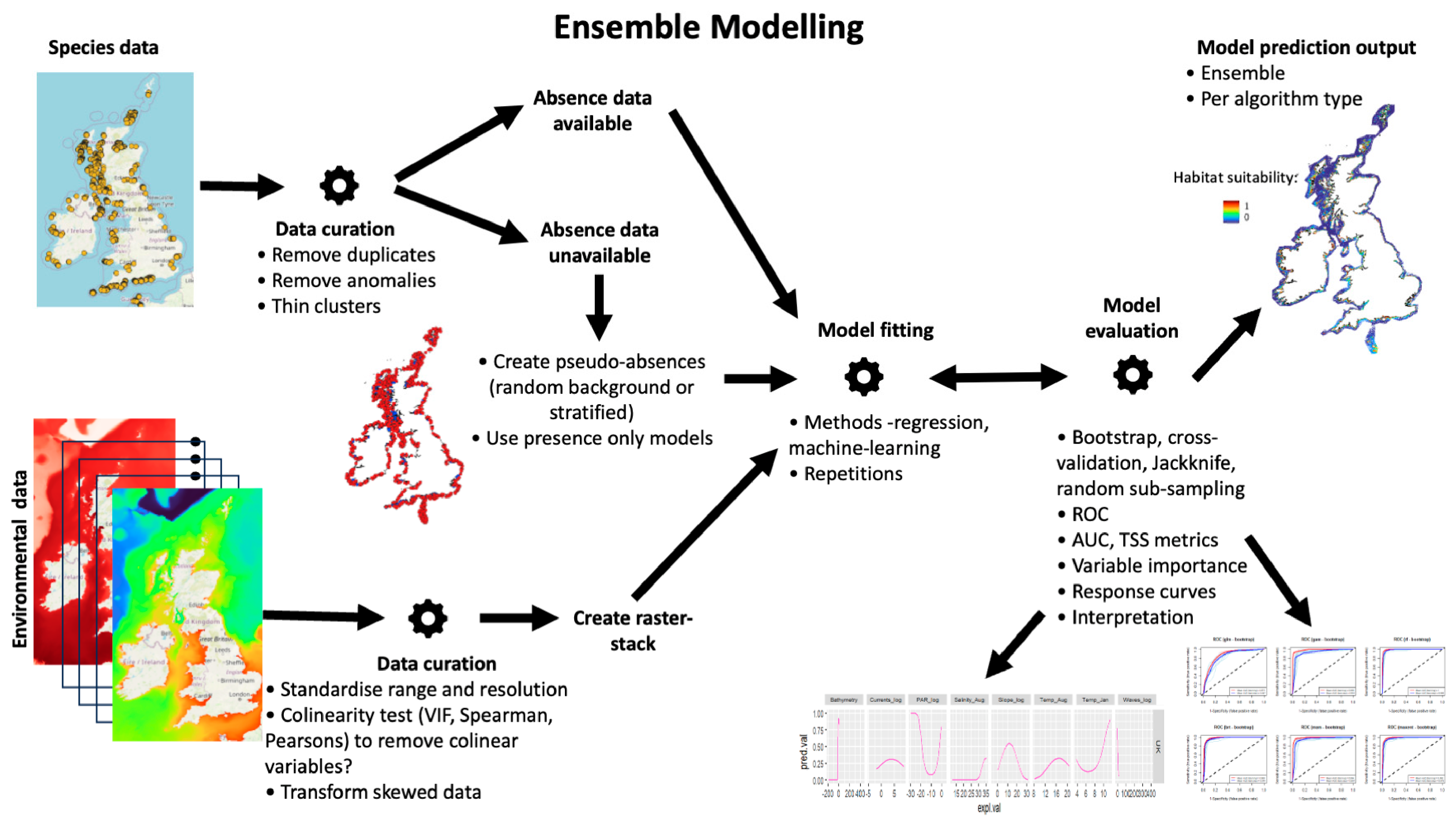
For this study, we used a range of machine-learning and statistical algorithms to investigate how environmental conditions explain seagrass presence between sites [21,22]. Generalised Linear Models (GLM) were included in the ensemble to assess performance for later transferability tests, along with Generalised Additive Models (GAM), Random Forest (RF), Boosted Regression Trees (BRT), Multivariate Adaptive Regression Splines (MARS), and Maximum Entropy (MaxEnt). All ensemble HSMs were created using the ‘sdm’ package [23] in R (v4.0.2). The models followed the formula of seagrass presence as a function of the predictor variables (a stack of the environmental variable layers) using the different approaches, repeated ten times per approach (Figure 2). As only presence data was available, randomly selected ‘background’ points were formulated within the geographical spatial range of the model area and used as pseudo-absences with equal weighting to the presences at each site, as recommended, to produce improved model performance [45,46]. The model formula uses a resampling method for data partitioning of the presence point data, which is used to test and validate the model using a bootstrapping method in this case for model evaluation. Bootstrapping uses a repeat sampling with replacement method, each time a sample with equal size as the original data is drawn and used for training data. The observations that are not selected are used for the evaluation at each run [23]. Predictions of presence are then created for each approach (GLM, etc.) and each run (repetition) and combined within an ensemble model, which takes a weighted average of the predicted suitability from all runs. Predictions of habitat suitability were mapped as a spatial raster layer indicating an occurrence probability (interpreted as habitat suitability) ranging from 0 to 1. Variable importance was calculated using the ‘getVarImp’ function in the ‘sdm’ package in R. This calculates Variable importance using two permutation-based methods: (a) Correlation-based and (b) AUC-based [23].
Species habitat associations can be simplified to positive, negative or ambivalent relationships with their resources, risks and conditions [26]. Generalised Linear Models (GLM) can be applied to describe these correlative relationships, allowing simple interpretation of these relationships. Previous studies have found good transferability for algorithms such as GLM over other more complex models, whereby transferability is reduced through overfitting [33]. Therefore, to further explore and compare variable influence on seagrass presence and transferability of HSM between site areas, GLMs were chosen. Quadratic binomial GLMs (logit link) were found to perform the best based on AIC scores when compared with linear and polynomial terms. GLMs were estimated for each site using original presence and pseudoabsence (background points) used for the ensemble models (using the ‘sdm’ package) previously carried out for each site area using all eight environmental variables. GLMs performed well within the ensemble methods and therefore justified testing for transferability and allowed trends in variables associated with seagrass presence to be easily interpreted. Models were applied between sites using the ‘ROCR’ package in R [47] to assess transferability and scalability of HSM using AUC, the Area Under the ROC Curve (Receiver Operator Curves [48]), and Nagelkerke’s (Pseudo-)R2 (a measure of the explained variance) as the main metrics for comparison and performance. All R code is available in Supporting Information.
All analyses in the Methods were performed using R Statistical Software (v4.0.2 [49]) and spatial data visualisation and manipulation using QGIS (v3.20.3 [50]). The script is available via the Zenodo repository (https://doi.org/10.5281/zenodo.23394541).
Figure 2.
Steps involved in ensemble habitat suitability modelling showing British Isles and Ireland example for Zostera marina. Species presence data and environmental data layers are sourced and edited into a suitable format for the software or packages used. Models are fitted using a range of algorithm types and an ensemble model using weighted averages of all model runs is created. The final model and all model runs can be evaluated using a number of methods and outputs for interpretation such as AUC, i.e., the Area Under ROC Curve (Receiver Operator Curves, [48]), TSS (True Summary Statistic, [51]). Models can be re-run/re-fitted at this point if any evaluation outputs are shown to be strange or uninterpretable.
3. Results
Occurrence data compilation and processing after removing duplicates resulted in 2315 presences and 2315 pseudo-absence records, which were used to model the distribution of Z. marina across all case study sites and the UK and Ireland. To compare spatial scale between sites, the spatial area modelled was calculated together with the number of presence points per site to provide a ratio of presences per square kilometre (Table 2).
Table 2.
Area in square kilometres per case study site and UK and Ireland to give scale of study areas (coastal sea used for models with land removed) and the corresponding number of seagrass presence data points utilised for HSM available at time of study. Areas were calculated using the Field Calculator function in QGIS.
The distribution models achieved high predictive performance for all model methods, with average AUC > 0.88 and TSS and COR > 0.7 (see Table 3).
Table 3.
Results from the ensemble models per case study location showing the average from 10 runs per model method. All variables are logged: currents, waves, PAR and slope. Metrics include AUC (Area Under the Curve), COR (Correlation coefficient), TSS (True Summary Statistic) and Deviance (explained).
Ensemble models were run successfully for all site areas apart from Porthdinllaen, where some GAMs did not converge. This is likely due to the small spatial scale of the model areas, resulting in little change in detectable environmental conditions.
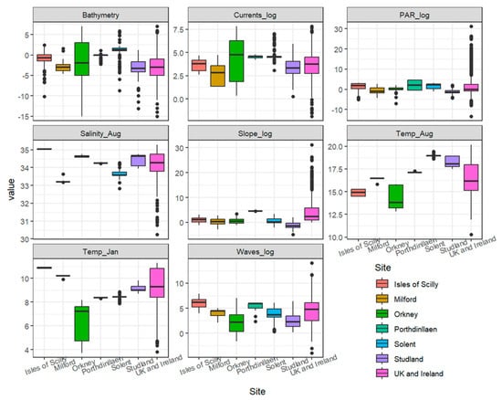
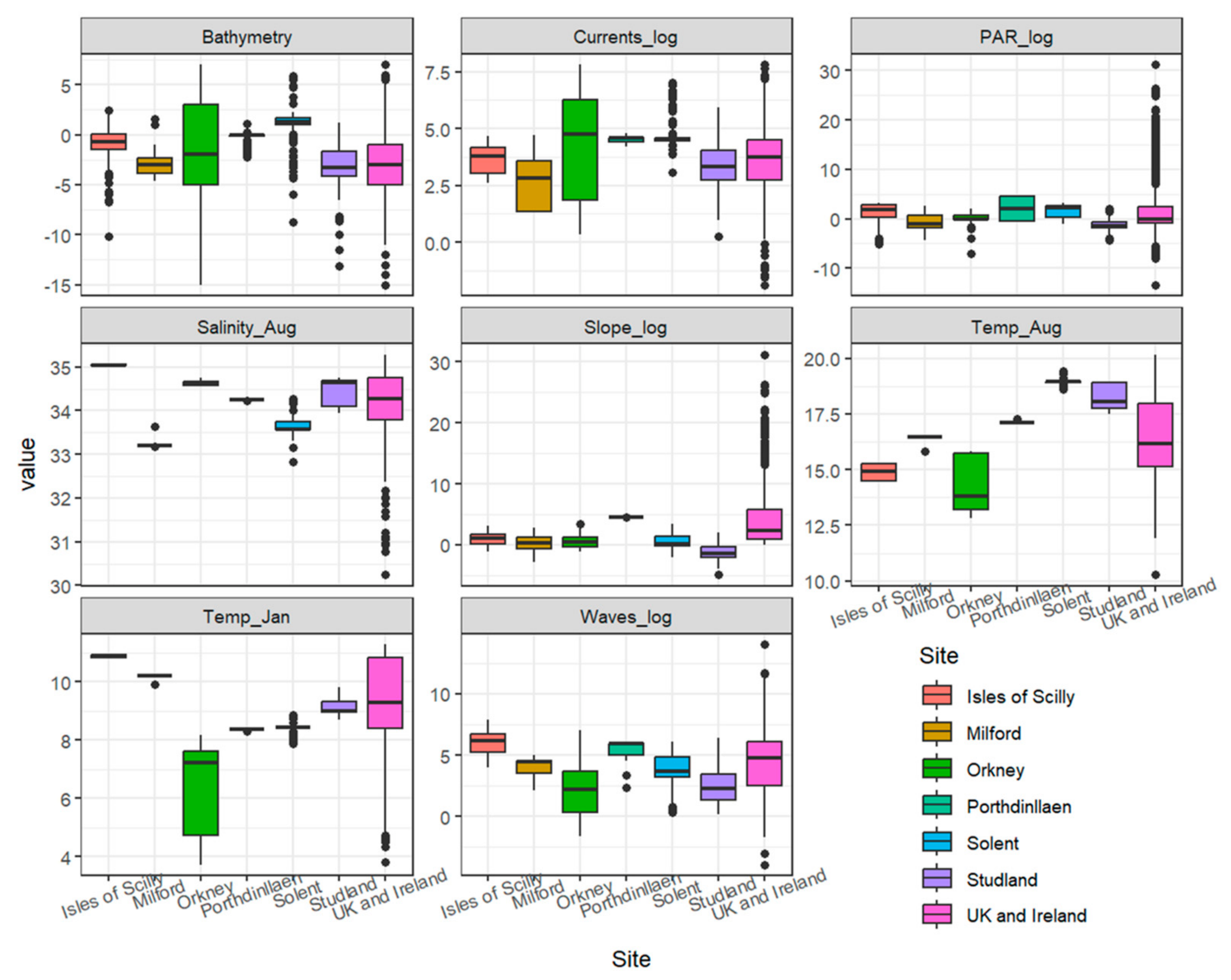
Environmental conditions showed clear spatial variability across sites (Figure 3) and in the UK models. Bathymetry varied strongly, with Orkney showing the deepest values (≈−15 m). Mean kinetic energy from currents at the seabed was highest in Orkney, Porthdinllaen and Solent, with values ranging from 1 to 2473 N.m2.s−1. PAR showed moderate differences among sites, with UK averages exhibiting the largest spread due to high variability compared with all sites. Salinity in August remained at a consistent range from 33 and 35 PSU across all sites, whereas slope values were consistently low. August temperature was highest in Studland Bay (≈18–19 °C) and Solent (≈17–18 °C). January temperature showed a similar pattern, with the Isles of Scilly and Studland Bay recording the warmest winter conditions (≈10–11 °C), coinciding with peak wave energy levels. Overall, southern sites showed warmer temperatures, higher wave exposure, and steeper slopes, whereas northern sites (e.g., Orkney) were characterised by lower temperatures and variable current regimes.
Figure 3.
Environmental ranges for HSM sites and UK and Ireland for Zostera marina presence points using variables used in all models, including bathymetry, log mean kinetic energy at the seabed due to currents, log mean kinetic energy from waves, log PAR at the seabed, mean salinity for August, mean temperature for January and August and log slope (see Table S2 for raw values). Midlines represent the median, the box represents the interquartile range and points equal outliers.
The environmental predictors used to model the distribution of Z. marina are displayed with ranges and mean values for each site area in Figure 3 (Table S3).
3.1. Heterogeneity Between Sites
The importance of predictors from the ensemble models varied between local sites and the UK and Ireland (Figure S2, Table S4). For the large-scale British Isles model and Studland, bathymetry was the most important variable, followed by PAR (ranged between 10 and 60%). PAR was the most important variable for Orkney, followed by salinity. This predictor was also the most important for Solent and Porthdinllaen areas and sea temperature (January) for Milford Haven and Isles of Scilly. Overall, slope, currents, and wave energy were the least important factors in explaining the distribution of Z. marina.
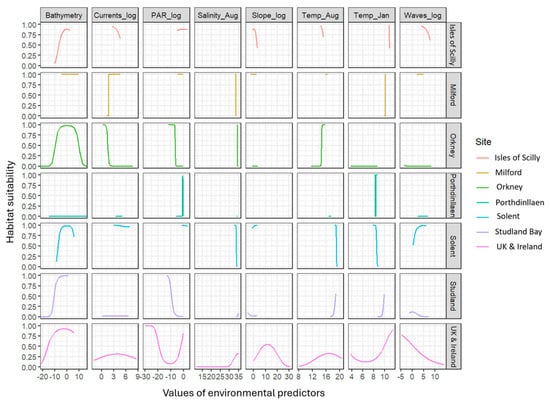
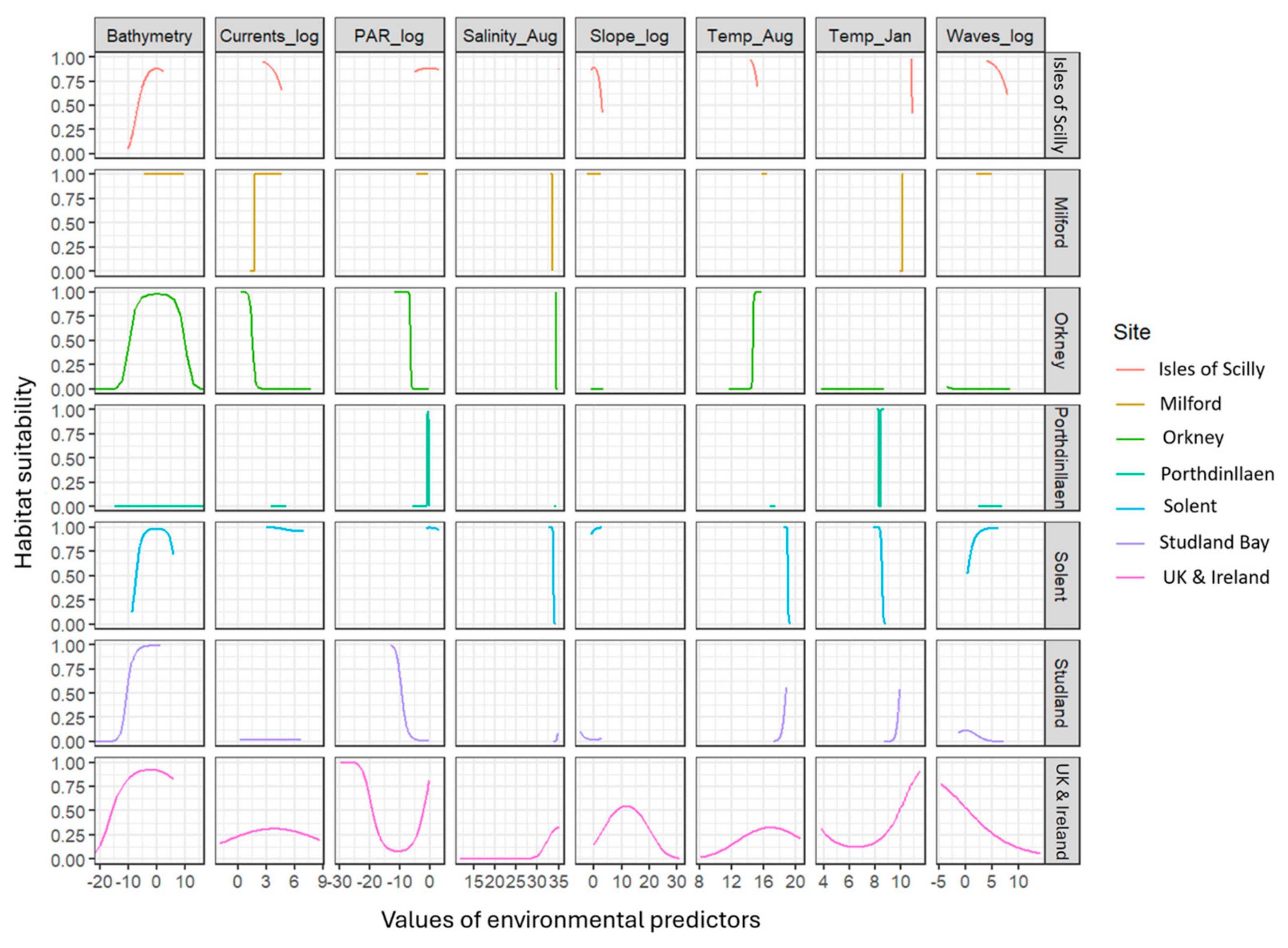
Heterogeneity between sites is also displayed by the differences in response curves calculated for seagrass suitability using GLMs (Figure 4). Predicted values for seagrass suitability (0–1) are plotted against the explanatory values of the environmental predictors and show different patterns between sites. Overall, at the UK scale and case study sites, the models showed that seagrass suitability increased with low bathymetry between −10 m and 5 m, PAR values from 1 to 20 mol m−2 day−1, salinity in August between 33 and 35 PSU, August temperatures above 16 °C and January temperatures above 8 °C. Additionally, the suitability declined with increasing slope, current velocity, and wave energy. In Orkney and Solent, bathymetry was the dominant predictor, with suitability sharply increasing at mid-depths. Orkney also showed a strong positive response to January temperatures above 6 °C, while Solent exhibited increased suitability at higher PAR levels. Salinity in August contributed positively but only within a narrow optimal range (33–35 PSU), particularly for sites like Studland and Isles of Scilly, but only really visible at the UK and Ireland scale owing to the low resolution of the data. Currents, wave energy and slope had limited effects at most locations (Figure 4), with flat or slightly declining response curves, suggesting low sensitivity to hydrodynamics. However, interpretation from the response curves should be taken with caution, as many of the site-specific response curves only show a partial response. This will be due to the low resolution of some of the variable data obscuring finer detail of trends and showing low variation across a smaller spatial scale. Bathymetry responses for Solent and Orkney highlight the inclusion of intertidal data points having an effect at these sites and the heterogeneity between sites overall.
Figure 4.
Response variables for each case study site and UK and Ireland GLM HSM. Predicted values (0–1) for seagrass suitability are plotted against explanatory values for the environmental variables obtained from the GLMs. Units for environmental predictors are found in Table S2.
3.2. Transference Across Scales
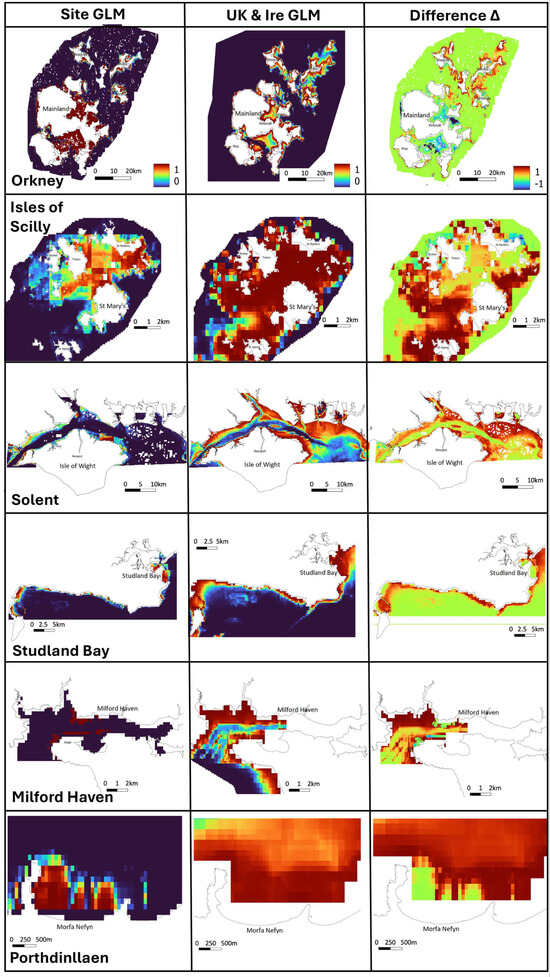
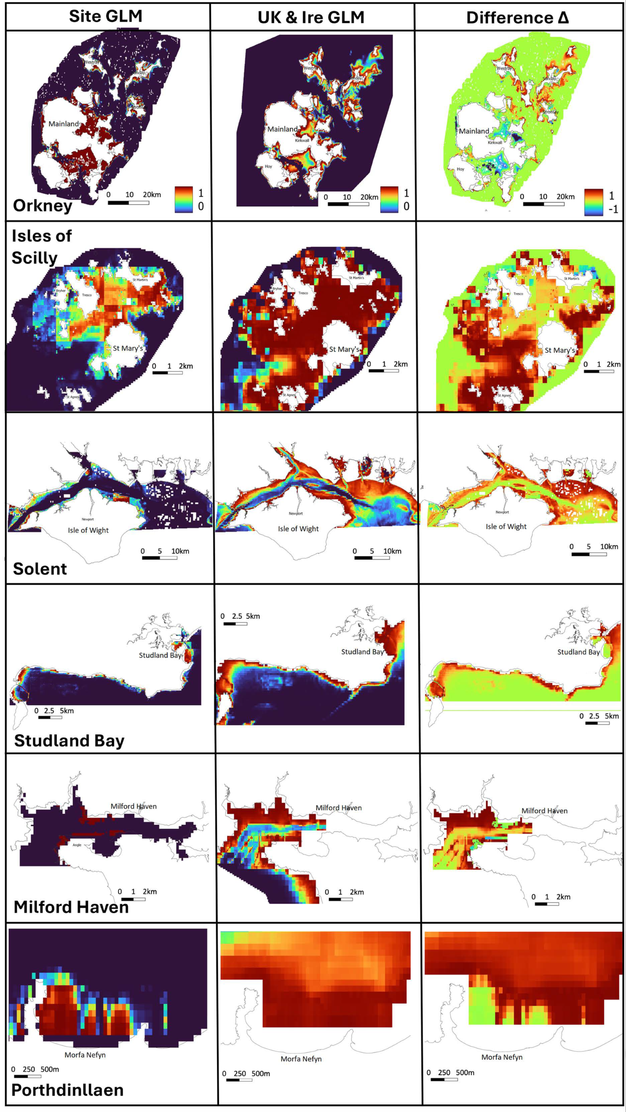
The GLM results for predicting seagrass habitat suitability at each case study site and then for the whole UK and Ireland are displayed as heatmaps (Figure 5). The local-scale GLM predicted probability (‘suitability’) at each site was then subtracted from the broad-scale (UK and Ireland) GLM to show differences in predictions on a scale of −1 to +1. At the local scale, the broad-scale GLM appears to overpredict especially for smaller areas (Table 2) such as Isles of Scilly, Milford Haven and Porthdinllaen, with larger regions of positive differences in red (Figure 5, right-hand column).
Figure 5.
Outputs from HSM using GLM at case study scale (left-hand column), using the UK and Ireland scale model (middle column) and showing the difference (right-hand column) by subtracting the probability values for the local scale from the UK-wide model results (values −1 to 1). For the last two sites, the UK model data was not interpolated to the same level as the local scale data, so there is some discrepancy in coverage.
3.3. Transference Across Space
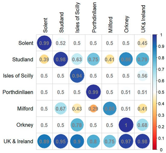
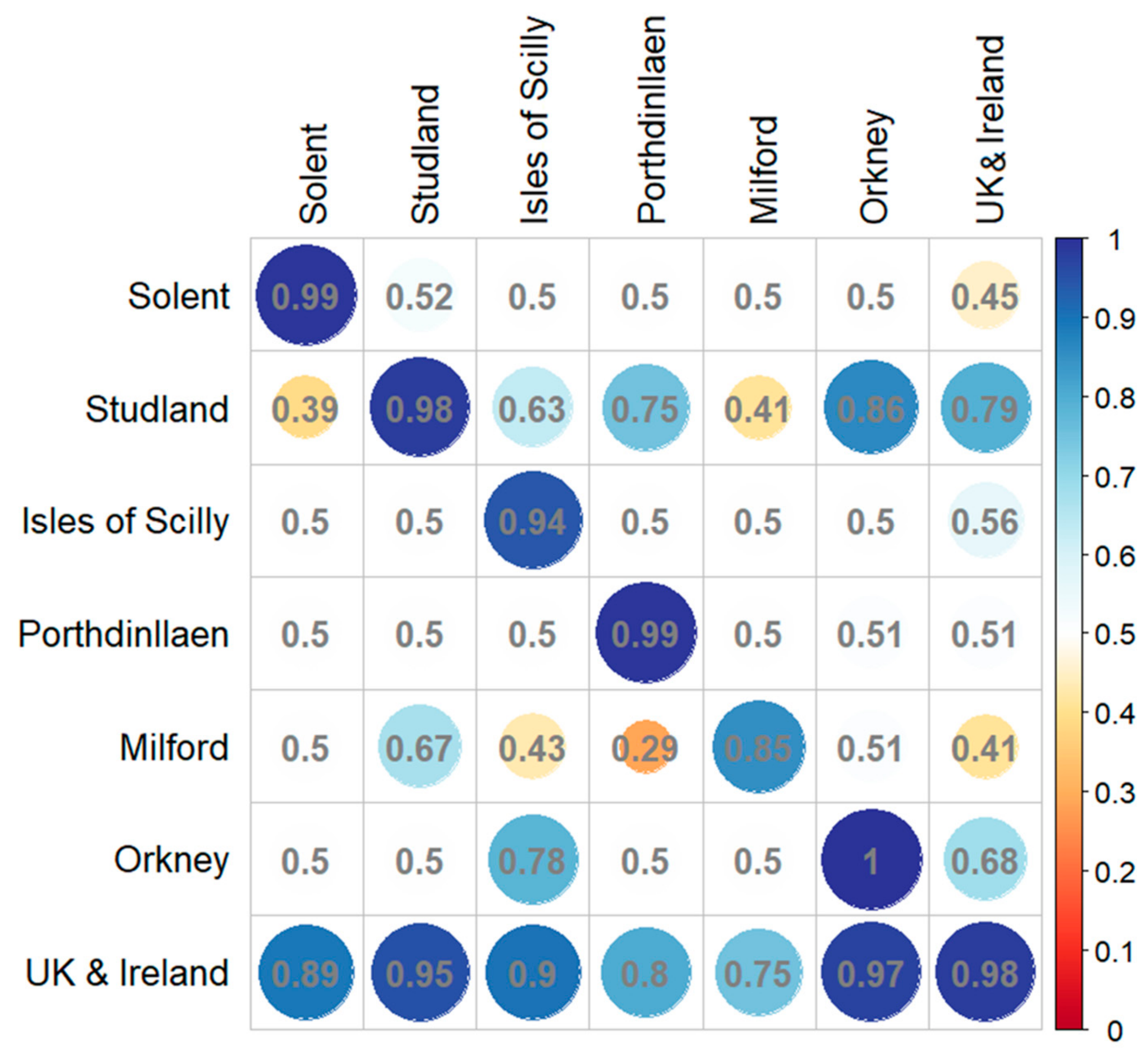
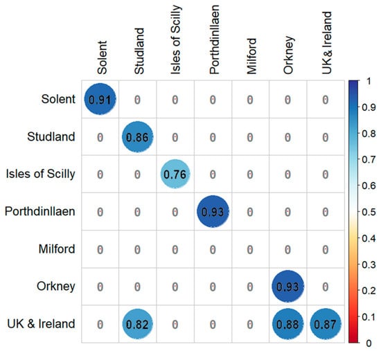
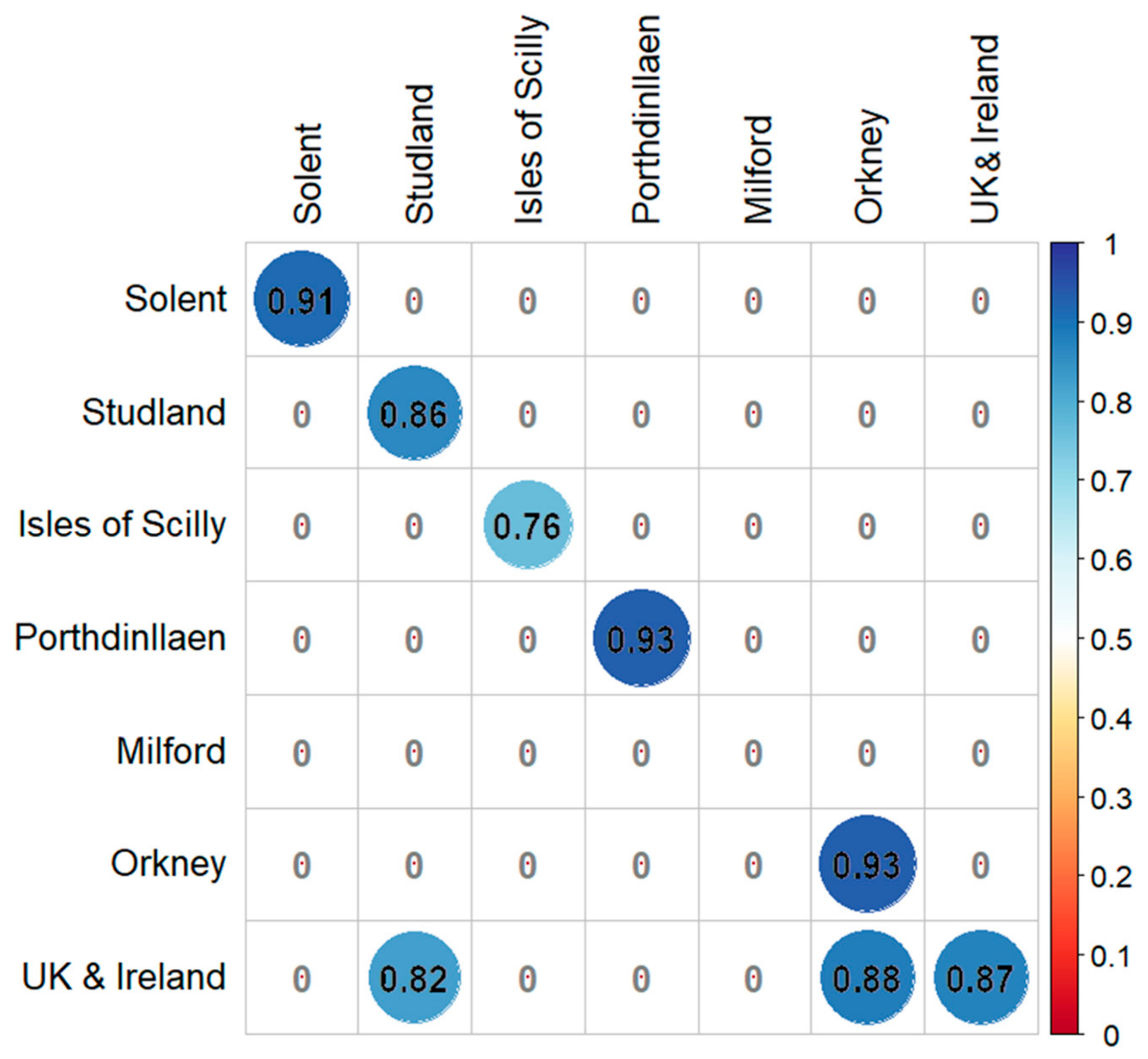
The UK and Ireland model successfully transferred to many other sites with excellent AUC scores (>0.9) for Studland, Isles of Scilly and Orkney, and good (>0.7) for Porthdinllaen and Milford Haven (Figure 6). The GLM for Studland Bay had good AUC scores when applied to Porthdinllaen, Orkney and the UK and Ireland. The only other good score was the Orkney model when applied to Isles of Scilly (AUC 0.78). This pattern was also shown when Root Mean Square Error was calculated for each model transfer (Figure S2). Nagelkerke’s R2 was calculated for further interpretation of model performance and transference across sites (Figure 7). All models performed well according to the R2 metric (>0.7) except for Milford Haven. As for transference, R2 values confirm some of the patterns shown by the AUC scores, albeit only for the UK and Ireland model when applied to Studland Bay (0.82) and Orkney (0.88).
Figure 6.
AUC scores for GLM model transferability are shown as a correlation plot using AUC scores shown in Table 3. Circle size corresponds to the value (0–1) and the colour scale on the right side of the plot, red for lower fit (closer to 0) to blue for higher fit (closer to 1).
Figure 7.
Nagelkerke’s R2 scores for GLM model transferability shown as a correlation plot. Circle size corresponds to the value (0–1), and colour is scaled on the right side of the plot, red for lower fit (closer to 0) to blue for higher fit (closer to 1). Many scores were highly negative values showing full model performing significantly worse than the null model. These values are displayed as ‘0’ in the plot as a lower cut-off value for presentation purposes.
4. Discussion
This study provides important assessments of model transferability for eelgrass across different spatial scales. Using relevant environmental predictors, we applied ensemble and generalised linear models (GLMs) across six sites and a broad UK and Ireland extent. Models consistently performed well within their respective spatial domains, indicating strong site-specific fits. However, transferability across scales was limited. Notably, large-scale models transferred more effectively to local sites than the reverse, likely because they captured broader environmental gradients. Despite this, the national model tended to over-predict habitat suitability in shallow coastal areas, reflecting the important influence of depth-related variables such as bathymetry and PAR. In contrast, local-scale models, calibrated on narrower environmental ranges, produced more ecologically realistic predictions and are therefore better suited to inform site-specific management and restoration efforts.
The distribution patterns predicted by the model were largely shaped by bathymetry, with light availability as a secondary but important factor. Wave energy had relatively minor effects in the models, but this likely reflects the spatial resolution of the available data, as higher-resolution wave information has been shown to significantly improve predictions of seagrass presence in HSMs [24]. The eelgrass Zostera marina, like many other plant species, exhibits considerable plasticity, enabling it to thrive across a wide range of environmental conditions [52]. It occurs in sheltered estuaries and lagoons as well as along more exposed coasts. Across UK meadows, populations lie well within the species’ biogeographical temperature and salinity ranges and are not expected to be limiting factors. However, temperature and salinity were found to be important predictors at some case study sites, including the Isles of Scilly and Milford Haven. Exceptions occur where Z. marina extends into upper estuaries with reduced salinity or in areas affected by local thermal inputs, such as power station cooling water discharges and in some cases extending into the intertidal zone. Temperature in this case could be acting as a proxy for latitude and associated environmental gradient, just as bathymetry often does for light availability [53]. Consequently, light availability and hydrodynamic conditions are expected to play a greater role in shaping its distribution [54]. However, hydrological data at high enough resolution for shallow coastal waters is difficult to obtain without site-specific models used to create such data.
All models were developed using a biologically important range of environmental predictors, which can lead to differences in the relative importance of predictors when compared across regions. As a result, these models often fail to generalise when applied beyond their calibration area. This was evident in our analysis, where local HSMs showed limited transferability to other case study sites—except for instances such as the Studland Bay and Orkney Isles GLMs, which performed moderately well when transferred according to AUC scores. For example, the Orkney model transferred better to the Isles of Scilly according to AUC and RMSE scores, possibly due to both being offshore island groups with comparable coastal conditions, whereas the reverse transfer showed poorer results. These findings reflect the strong influence of localised environmental gradients, such as sediment composition, light availability, and wave exposure, which vary significantly across sites and constrain model applicability [55,56]. Limited model transferability has been noted in previous research, highlighting the challenges of applying habitat suitability models beyond their original spatial context due to environmental variability and data constraints [57]. These findings reinforce the importance of region-specific modelling approaches for effective seagrass restoration planning.
However, the broad-scale model does appear to over-predict suitability around shallower coastlines, as bathymetry and photosynthetically active radiation (PAR)—both directly related to depth—were found to be the most important variables in explaining overall seagrass presence. This could also be due to the relatively low resolution of these predictors, which could be missing finer environmental factors such as exposure or substrate that were not integrated. Local-scale models, estimated over smaller sections of the environmental gradient, can therefore exhibit different slope directions or reduced predictor influence, resulting in limited generality when transferred to broader contexts. In this study, the models estimated at smaller spatial scales for the case study areas appear to provide more realistic predictions of suitable seagrass habitat when compared with the UK and Ireland model (shown in dark red). Similar patterns of broad-scale overestimation have been noted elsewhere [37,58], underscoring the challenges of scaling up habitat suitability models without accounting for regional environmental heterogeneity.
Although the models showed high performance in Zostera marina distribution across the UK and Ireland, certain limitations must be acknowledged, as they may introduce uncertainty into the predicted outcomes. To ensure model transferability, environmental predictors needed to be consistent across both broad and local scales. As a result, the current distribution was estimated using a limited set of climatic variables. Incorporating additional environmental drivers could enhance model realism; however, some important data (e.g., substrate) were currently unavailable at sufficient spatial extent or resolution at the time of this study.
Additionally, presence records are often focussed on established meadows, which do not consider the changing needs of a species throughout its life cycle, particularly relevant to ecosystem engineers such as Z. marina, which are known to modify their environment, for example by slowing water movement [59,60]. Records and genetic analysis have aged of some Z. marina meadows at over 80 years old [61,62]; with the current rate of environmental change, directly due to coastal modification and through changing climate, linking current records of established meadows does not capture the conditions during site colonisation.
Our assessment of current distributions of Zostera marina across the UK and Ireland from the compiled occurrence data and its subsequent modelled potential, highlights the significant role this species can play in advancing national restoration and climate resilience goals. While Z. marina meadows are relatively widespread, our models reveal that their localised persistence needs to be considered under climatic and local environmental pressures. This emphasises the urgent need for targeted conservation and restoration strategies that enhance meadow resilience and secure the valuable ecosystem services these habitats provide—such as carbon sequestration, coastal protection, and biodiversity support.
Integrating Z. marina restoration into broader national policy frameworks, including Blue Carbon strategies and marine spatial planning, could help align local restoration efforts with international climate and biodiversity targets. Such measures, when combined with improved environmental data and regionally tailored habitat models, can guide more effective restoration outcomes.
5. Conclusions
Habitat suitability modelling is a useful tool for determining where species are most likely to survive based on environmental predictor variables and is also useful for site selection for restoration work. Although transferability of models can be limited, broad-scale models still provide a good starting point. In the case of Z. marina, the broad-scale model over-predicts suitability, but this at least at the first instance does not discount potentially suitable areas that could be overlooked by finer-scale, highly fitted models. Fine-tuning models to more specific locations is recommended to provide a secondary overlay that would improve justification of site selection by practitioners. However, it is important at this stage not to exclude any local site knowledge that would provide invaluable insight into local conditions that would be overlooked by the type of yearly/monthly averaged environmental data layers which often form the basis of HSMs and SDMs.
Supplementary Materials
The following supporting information can be downloaded at https://www.mdpi.com/article/10.3390/jmse14212018/s1: Table S1: Seagrass presence data sources and data type with date of acquisition; Table S2: Environmental variables used for HSM including data source and resolution; Table S3: Ranges and means for each environmental variable at the case study sites to show difference in environmental conditions where seagrass presence was found; Figure S1: Correlation plot for the variables used for ensemble models for all sites and UK & Ireland after removal of collinear variables with a variance inflation factor (VIF) exceeding the threshold of 0.9; Table S4: Variable importance (%) based on Correlation metric and AUC; Figure S2. RMSE (Root Mean Square Error) scores for GLM model transferability shown as correlation plot using RMSE scores shown in Table.
Author Contributions
C.M.B. wrote the manuscript and analysed the data. L.G., C.D., M.L., B.S., R.K.F.U. and J.C.B. wrote and edited the manuscript. M.L., B.S. and J.C.B. contributed to analysis methods. J.C.B. and C.M.B. conceived and designed the research. All authors have read and agreed to the published version of the manuscript.
Funding
This research was funded by NERC (Natural Environment Research Council) grant number NE/V01711X/1 and by the German Federal Ministry of Education and Research (BMBF) with grant number 03F0859D as well as the German Federal Ministry of Research, Technology and Space (BMFTR) and the German Federal Ministry for the Environment, Climate Action, Nature Conservation and Nuclear Safety (BMUKN) with grant number 03F0978D.
Data Availability Statement
This study was conducted using E.U. Copernicus Marine Service Information: https://doi.org/10.48670/moi-00016 Global Ocean Physics Analysis and Forecast. E.U. Copernicus Marine Service Information (CMEMS). Marine Data Store (MDS). DOI: 10.48670/moi-00016 (Accessed on 1 March 2022). Licensed under CC-BY 4.0—please use attribution statement: licensed under CC-BY 4.0 from the European Marine Observation and Data Network (EMODnet) Seabed Habitats initiative (www.emodnet-seabedhabitats.eu, accessed on 1 March 2022), funded by the European Commission.
Acknowledgments
This study was part of the ReSOW (Restoring Seagrass for Ocean Wealth) project funded by NERC (Natural Environment Research Council).
Conflicts of Interest
The authors declare no conflict of interest.
References
- Duarte, C.M.; Losada, I.J.; Hendriks, I.E.; Mazarrasa, I.; Marbà, N. The role of coastal plant communities for climate change mitigation and adaptation. Nat. Clim. Chang. 2013, 3, 961–968. [Google Scholar] [CrossRef] [Scilit]
- McMahon, L.; Ladd, C.J.T.; Burden, A.; Garrett, E.; Redeker, K.R.; Lawrence, P.; Gehrels, R. Maximizing blue carbon stocks through saltmarsh restoration. Front. Mar. Sci. 2023, 10, 1106607. [Google Scholar] [CrossRef] [Scilit]
- O’Leary, B.C.; Fonseca, C.; Cornet, C.C.; de Vries, M.B.; Degia, A.K.; Failler, P.; Furlan, E.; Garrabou, J.; Gil, A.; Hawkins, J.P.; et al. Embracing nature-based solutions to promote resilient marine and coastal ecosystems. Nat.-Based Solut. 2023, 3, 100044. [Google Scholar] [CrossRef] [Scilit]
- do Amaral Camara Lima, M.; Bergamo, T.F.; Ward, R.D.; Joyce, C.B. A review of seagrass ecosystem services: Providing nature-based solutions for a changing world. Hydrobiologia 2023, 850, 2655–2670. [Google Scholar] [CrossRef] [Scilit]
- Unsworth, R.K.F.; Williams, B.; Jones, B.L.; Cullen-Unsworth, L.C. Rocking the boat: Damage to eelgrass by swinging boat moorings. Front. Plant Sci. 2017, 8, 262. [Google Scholar] [CrossRef] [Scilit] [PubMed]
- Gamble, C.; Glover, A.; Debney, A.; Bertelli, C.; Green, B.; Hendy, I.; Lilley, R.; Nuuttila, H.; Potouroglou, M.; Ragazzola, F.; et al. Seagrass Restoration Handbook: UK and Ireland; Zoological Society of London: London, UK, 2021. [Google Scholar]
- Burgess, H.; Adnitt, C.; Armstrong, S.; Ausden, M.; Austin, W.; Balke, T.; Burden, A. Saltmarsh Restoration Handbook: UK & Ireland; Environment Agency: Bristol, UK, 2021. [Google Scholar]
- Ridge, J.T.; Rodriguez, A.B.; Fodrie, F.J. Salt marsh and fringing oyster reef transgression in a shallow temperate estuary: Implications for restoration, conservation and blue carbon. Estuaries Coasts 2017, 40, 1013–1027. [Google Scholar] [CrossRef] [Scilit]
- Preston, J.; Debney, A.; Gamble, C.; Hardy, M.J.; Underwood, G.J.C.; Garbutt, A.; Harley, J.; Baker, R.; Dunk, R.M.; Grigg, M.; et al. Seascape connectivity: Evidence, knowledge gaps and implications for temperate coastal ecosystem restoration practice and policy. npj Ocean Sustain. 2025, 4, 33. [Google Scholar] [CrossRef] [Scilit] [PubMed]
- Greiner, J.T.; McGlathery, K.J.; Gunnell, J.; McKee, B.A. Seagrass restoration enhances “blue carbon” sequestration in coastal waters. PLoS ONE 2013, 8, e72469. [Google Scholar] [CrossRef] [Scilit] [PubMed]
- Green, A.E.; Unsworth, R.K.F.; Chadwick, M.A.; Jones, P.J.S. Historical analysis exposes catastrophic seagrass loss for the United Kingdom. Front. Plant Sci. 2021, 12, 629962. [Google Scholar] [CrossRef] [Scilit] [PubMed]
- Bertelli, C.M.; Robinson, M.T.; Mendzil, A.F.; Pratt, L.R.; Unsworth, R.K.F. Finding some seagrass optimism in Wales, the case of Zostera Noltii. Mar. Pollut. Bull. 2018, 134, 216–222. [Google Scholar] [CrossRef] [Scilit] [PubMed]
- Garmendia, J.M.; Rodríguez, J.G.; Borja, Á.; Pouso, S.; del Campo, A.; Galparsoro, I.; Fernandes-Salvador, J.A. Restoring seagrass meadows in Basque estuaries: Nature-based solution for successful management. Nat.-Based Solut. 2023, 4, 100084. [Google Scholar] [CrossRef] [Scilit]
- Jayathilake, D.R.; Costello, M.J. A modelled global distribution of the seagrass biome. Biol. Conserv. 2018, 226, 120–126. [Google Scholar] [CrossRef] [Scilit]
- Gouvêa, L.; Fragkopoulou, E.; Legrand, T.; Serrão, E.A.; Assis, J. Range map data of marine ecosystem structuring species under global climate change. Data Brief 2024, 52, 110023. [Google Scholar] [CrossRef] [Scilit] [PubMed]
- Gouvêa, L.; Fragkopoulou, E.; Araújo, M.B.; Serrão, E.A.; Assis, J. Seagrass biodiversity under the latest-generation scenarios of projected climate change. J. Biogeogr. 2025, 52, 172–185. [Google Scholar] [CrossRef] [Scilit]
- Gouvêa, L.P.; Krause-Jensen, D.; Duarte, C.M.; Assis, J. Projected impacts of future climate change on the aboveground biomass of seagrasses at global scale. Sci. Total Environ. 2025, 966, 178680. [Google Scholar] [CrossRef] [Scilit] [PubMed]
- Zhou, J.; Wang, Q.; Zhao, W.; Yu, D.; Guan, S. Habitat suitability analysis of eelgrass Zostera marina L. in the subtidal zone of Xiaoheishan Island. Chin. J. Oceanol. Limnol. 2016, 34, 69–78. [Google Scholar] [CrossRef] [Scilit]
- Elith, J.; Leathwick, J.R. Species distribution models: Ecological explanation and prediction across space and time. Annu. Rev. Ecol. Evol. Syst. 2009, 40, 677–697. [Google Scholar] [CrossRef] [Scilit]
- Melo-Merino, S.M.; Reyes-Bonilla, H.; Lira-Noriega, A. Ecological niche models and species distribution models in marine environments: A literature review and spatial analysis of evidence. Ecol. Model. 2020, 415, 108837. [Google Scholar] [CrossRef] [Scilit]
- Bertelli, C.M.; Stokes, H.J.; Bull, J.C.; Unsworth, R.K.F. The use of habitat suitability modelling for seagrass: A review. Front. Mar. Sci. 2022, 9, 997831. [Google Scholar] [CrossRef] [Scilit]
- Valle, M.; van Katwijk, M.M.; de Jong, D.J.; Bouma, T.J.; Schipper, A.M.; Chust, G.; Benito, B.M.; Garmendia, J.M.; Borja, Á. Comparing the performance of species distribution models of Zostera marina: Implications for conservation. J. Sea Res. 2013, 83, 56–64. [Google Scholar] [CrossRef] [Scilit]
- Naimi, B.; Araújo, M.B. sdm: A reproducible and extensible R platform for species distribution modelling. Ecography 2016, 39, 368–375. [Google Scholar] [CrossRef] [Scilit]
- Elith, J.; Graham, C.H.; Anderson, R.P.; Dudík, M.; Ferrier, S.; Guisan, A.; Hijmans, R.J.; Huettmann, F.; Leathwick, J.R.; Lehmann, A.; et al. Novel methods improve prediction of species’ distributions from occurrence data. Ecography 2006, 29, 129–151. [Google Scholar] [CrossRef] [Scilit]
- Araújo, M.B.; Anderson, R.P.; Barbosa, M.A.; Beale, C.M.; Dormann, C.F.; Early, R.; Garcia, R.A.; Guisan, A.; Maiorano, L.; Naimi, B.; et al. Standards for distribution models in biodiversity assessments. Sci. Adv. 2019, 5, eaat4858. [Google Scholar] [CrossRef] [Scilit] [PubMed]
- Matthiopoulos, J.; Fieberg, J.R.; Aarts, G. Species-Habitat Associations: Spatial Data, Predictive Models, and Ecological Insights; University of Minnesota Libraries Publishing: Minneapolis, MN, USA, 2023. [Google Scholar] [CrossRef] [Scilit]
- Schröder, B.; Richter, O. Are habitat models transferable in space and time? Z. Ökol. Naturschutz 1999, 8, 195–205. [Google Scholar]
- Roberts, D.R.; Bahn, V.; Ciuti, S.; Boyce, M.S.; Elith, J.; Guillera-Arroita, G.; Hauenstein, S.; Lahoz-Monfort, J.J.; Schröder, B.; Thuiller, W.; et al. Cross-validation strategies for data with temporal, spatial, hierarchical, or phylogenetic structure. Ecography 2017, 40, 913–929. [Google Scholar] [CrossRef] [Scilit]
- Peterson, A.T.; Papeş, M.; Eaton, M.; Soberón, J. Transferability and model evaluation in ecological niche modeling: A comparison of GARP and Maxent. Ecography 2007, 30, 550–560. [Google Scholar] [CrossRef]
- Arif, S.; MacNeil, M.A. Predictive models aren’t for causal inference. Ecol. Lett. 2022, 25, 1741–1745. [Google Scholar] [CrossRef] [Scilit] [PubMed]
- Franks, D.W.; Ruxton, G.D.; Sherratt, T. Ecology needs a causal overhaul. Biol. Rev. 2025, 100, 1950–1969. [Google Scholar] [CrossRef] [Scilit] [PubMed]
- Heikkinen, R.K.; Marmion, M.; Luoto, M. Does the interpolation accuracy of species distribution models come at the expense of transferability? Ecography 2012, 35, 276–288. [Google Scholar] [CrossRef] [Scilit]
- Werkowska, W.; Márquez, A.L.; Real, R.; Acevedo, P. A practical overview of transferability in species distribution modeling. Environ. Rev. 2017, 25, 127–133. [Google Scholar] [CrossRef] [Scilit]
- Nordlund, L.M.; Koch, E.W.; Barbier, E.B.; Creed, J.C. Seagrass ecosystem services and their variability across genera and geographical regions. PLoS ONE 2016, 11, e0163091. [Google Scholar] [CrossRef] [Scilit] [PubMed]
- Unsworth, R.K.F.; Bertelli, C.M.; Coals, L.; Cullen-Unsworth, L.C.; Den Haan, S.; Jones, B.J.; Rees, S.R.; Thomsen, E.; Wookey, A.; Walter, B. Bottlenecks to seed-based seagrass restoration reveal opportunities for improvement. Glob. Ecol. Conserv. 2023, 48, e02736. [Google Scholar] [CrossRef] [Scilit]
- Evans, A.J.; Ford, E.; Cullen-Unsworth, L. Connecting governance and practice views on the barriers and solutions to scaled seagrass restoration in the UK. Mar. Policy 2025, 180, 106781. [Google Scholar] [CrossRef] [Scilit]
- Bertelli, C.M.; Bennett, W.G.; Karunarathna, H.; Reeve, D.E.; Unsworth, R.K.F.; Bull, J.C. High-resolution wave data for improving marine habitat suitability models. Front. Mar. Sci. 2023, 9, 1004829. [Google Scholar] [CrossRef] [Scilit]
- Sand-Jensen, K. Biomass, net production and growth dynamics in an eelgrass (Zostera marina L.) population in vellerup vig, Denmark. Ophelia 1975, 14, 185–201. [Google Scholar] [CrossRef] [Scilit]
- Orth, R.J.; Moore, K.A. Seasonal and year-to-year variations in the growth of Zostera marina L. (eelgrass) in the lower Chesapeake bay. Aquat. Bot. 1986, 24, 335–341. [Google Scholar] [CrossRef] [Scilit]
- Blok, S.E.; Olesen, B.; Krause-Jensen, D. Life history events of eelgrass Zostera marina L. populations across gradients of latitude and temperature. Mar. Ecol. Prog. 2018, 590, 79–93. [Google Scholar] [CrossRef] [Scilit]
- Yesson, C.; Bush, L.E.; Davies, A.J.; Maggs, C.A.; Brodie, J. The distribution and environmental requirements of large brown seaweeds in the British isles. J. Mar. Biol. Assoc. United Kingd. 2015, 95, 669–680. [Google Scholar] [CrossRef] [Scilit]
- Dormann, C.F.; Elith, J.; Bacher, S.; Buchmann, C.; Carl, G.; Carré, G.; Marquéz, J.R.G.; Gruber, B.; Lafourcade, B.; Leitão, P.J.; et al. Collinearity: A review of methods to deal with it and a simulation study evaluating their performance. Ecography 2013, 36, 27–46. [Google Scholar] [CrossRef] [Scilit]
- Naimi, B.; Hamm, N.A.S.; Groen, T.A.; Skidmore, A.K.; Toxopeus, A.G. Where is positional uncertainty a problem for species distribution modelling? Ecography 2014, 37, 191–203. [Google Scholar] [CrossRef] [Scilit]
- Guisan, A.; Thuiller, W.; Zimmermann, N.E. Habitat Suitability and Distribution Models: With Applications in R; Cambridge University Press: Cambridge, UK, 2017. [Google Scholar] [CrossRef] [Scilit]
- Barbet-Massin, M.; Jiguet, F.; Albert, C.H.; Thuiller, W. Selecting pseudo-absences for species distribution models: How, where and how many? Methods Ecol. Evol. 2012, 3, 327–338. [Google Scholar] [CrossRef] [Scilit]
- Liu, C.; Newell, G.; White, M. The effect of sample size on the accuracy of species distribution models: Considering both presences and pseudo-absences or background sites. Ecography 2019, 42, 535–548. [Google Scholar] [CrossRef] [Scilit]
- Sing, T.; Sander, O.; Beerenwinkel, N.; Lengauer, T. ROCR: Visualizing classifier performance in R. Bioinformatics 2005, 21, 3940–3941. [Google Scholar] [CrossRef] [Scilit] [PubMed]
- Fielding, A.H.; Bell, J.F. A review of methods for the assessment of prediction errors in conservation presence-absence models. Environ. Conserv. 1997, 24, 38–49. [Google Scholar] [CrossRef] [Scilit]
- R Core Team. R: A Language and Environment for Statistical Computing; R Foundation for Statistical Computing: Vienna, Austria, 2022. [Google Scholar]
- QGIS Development Team. QGIS Geographic Information System. Open Source Geospatial Foundation Project. 2025. Available online: https://www.qgis.org (accessed on 1 March 2025).
- Allouche, O.; Tsoar, A.; Kadmon, R. Assessing the accuracy of species distribution models: Prevalence, kappa and the true skill statistic (TSS). J. Appl. Ecol. 2006, 43, 1223–1232. [Google Scholar] [CrossRef] [Scilit]
- Bertelli, C.M.; Bull, J.C.; Cullen-Unsworth, L.C.; Unsworth, R.K.F. Unravelling the spatial and temporal plasticity of eelgrass meadows. Front. Plant Sci. 2021, 12, 664523. [Google Scholar] [CrossRef] [Scilit] [PubMed]
- Stevens, A.W.; Lacy, J.R. The influence of wave energy and sediment transport on seagrass distribution. Estuaries Coasts 2012, 35, 92–108. [Google Scholar] [CrossRef] [Scilit]
- Krause-Jensen, D.; Pedersen, M.F.; Jensen, C. Regulation of eelgrass (Zostera marina) cover along depth gradients in Danish coastal waters. Estuaries 2003, 26, 866–877. [Google Scholar] [CrossRef] [Scilit]
- Nielsen, S.; Sand-Jensen, K.; Borum, J.; Geertz-Hansen, O. Depth colonization of eelgrass (Zostera marina) and macroalgae as determined by water transparency in Danish coastal waters. Estuaries 2002, 25, 1025–1032. [Google Scholar] [CrossRef] [Scilit]
- Erftemeijer, P.L.; van Gils, J.; Fernandes, M.B.; Daly, R.; van der Heijden, L.; Herman, P.M. Habitat suitability modelling to improve understanding of seagrass loss and recovery and to guide decisions in relation to coastal discharge. Mar. Pollut. Bull. 2023, 186, 114370. [Google Scholar] [CrossRef] [Scilit] [PubMed]
- Grigg, M.; Cucknell, A.; Marten, K.; Cox, T.; Yesson, C. Habitat suitability modelling for restoration of intertidal seagrass, Zostera noltei: A case study from the Greater Thames Estuary, UK. Estuar. Coast. Shelf Sci. 2025, 312, 109039. [Google Scholar] [CrossRef] [Scilit]
- Castle, L.; Pinder, J.; Lillis, H.; Manca, E. Using an Ensemble Modelling Approach to Predict Suitable Habitat for Zostera marina Beds, Modiolus modiolus Beds and Sabellaria spinulosa Reefs in UK Waters; JNCC Report 718; Joint Nature Conservation Committee: Peterborough, UK, 2022. [Google Scholar]
- Reidenbach, M.A.; Thomas, E.L. Influence of the seagrass, Zostera marina, on wave attenuation and bed shear stress within a shallow coastal bay. Front. Mar. Sci. 2018, 5, 397. [Google Scholar] [CrossRef] [Scilit]
- Koch, E.W.; Sanford, L.P.; Chen, S.-N.; Shafer, D.J.; Smith, J.M. Waves in Seagrass Systems: Review and Technical Recommendations; System-Wide Water Resources Research Program and Submerged Aquatic Vegetation Restoration Research Program, Engineer Research and Development Center: Gunpowder, MD, USA, 2006. [Google Scholar]
- Reusch, T.B.; Boström, C.; Stam, W.T.; Olsen, J.L. An ancient eelgrass clone in the Baltic. Mar. Ecol. Prog. Ser. 1999, 183, 301–304. [Google Scholar] [CrossRef] [Scilit]
- Rhode, J.M.; Duffy, J.E. Relationships between bed age, bed size, and genetic structure in Chesapeake Bay (Virginia, USA) eelgrass (Zostera marina L.). Conserv. Genet. 2004, 5, 661–671. [Google Scholar] [CrossRef] [Scilit]

Disclaimer/Publisher’s Note: The statements, opinions and data contained in all publications are solely those of the individual author(s) and contributor(s) and not of MDPI and/or the editor(s). MDPI and/or the editor(s) disclaim responsibility for any injury to people or property resulting from any ideas, methods, instructions or products referred to in the content. |
© 2026 by the authors. Licensee MDPI, Basel, Switzerland. This article is an open access article distributed under the terms and conditions of the Creative Commons Attribution (CC BY) license.