


Abstract
Advances in AI are accelerating intelligent ship autonomy, yet robust trajectory tracking remains challenging under nonlinear dynamics and persistent environmental disturbances. Traditional model-based guidance becomes tuning-sensitive and loses robustness under strong disturbances, while data-driven approaches like reinforcement learning often suffer from poor generalization to unseen dynamics and brittleness in out-of-distribution conditions. To address these limitations, we propose a guidance architecture embedding a Large Language Model (LLM) directly within the closed-loop control system. Using in-context prompting with a structured Chain-of-Thought (CoT) template, the LLM generates adaptive k-step heading reference sequences conditioned on recent navigation history, without model parameter updates. A latency-aware temporal inference mechanism synchronizes the asynchronous LLM predictions with a downstream Model Predictive Control (MPC) module, ensuring dynamic feasibility and strict actuation constraints. In MMG-based simulations of the KVLCC2, our framework consistently outperforms conventional model-based baselines. Specifically, it demonstrates superior path-keeping accuracy, higher corridor compliance, and faster disturbance recovery, achieving these performance gains while maintaining comparable or reduced rudder usage. These results validate the feasibility of integrating LLMs as predictive components within physical control loops, establishing a foundation for knowledge-driven, context-aware maritime autonomy.
1. Introduction
The maritime industry is undergoing rapid technological transformation driven by advances in automation and intelligent control systems. At the center of this transition lies the concept of the Maritime Autonomous Surface Ship (MASS), a key enabling technology for improving the efficiency, safety, and sustainability of maritime operations. Recent advances in artificial intelligence (AI) and big data analytics have accelerated the development of intelligent ships by improving their autonomous perception and decision-making capabilities (Bai et al. [1]; Boretti [2]). As the complexity of control and decision-making for MASS continues to increase, Kim et al. [3] emphasized that advancing AI-based control technologies has become a critical requirement for the future development of MASS.
A primary control objective for MASS is to ensure stable tracking of a predefined trajectory. The trajectory-tracking problem aims to guarantee that an autonomous vessel follows a designated path while minimizing cross-track error (CTE) (Xu and Guedes Soares [4]). However, the marine environment is characterized by nonlinear dynamics affected by persistent disturbances such as wind and current. These unpredictable disturbances make accurate trajectory tracking difficult (Fossen [5]). They introduce nonlinearities in vessel motion and uncertainties in propulsion, thereby challenging the stability and robustness of conventional control systems.
Traditional guidance systems have largely evolved within the framework of model-based control (Fossen [5]). This approach relies on a vessel’s dynamic equations of motion to compute control inputs, offering a high degree of stability and predictability. Among these methods, Line-of-Sight (LOS) guidance remains one of the most widely used because of its simple structure and proven robustness (Fossen et al. [6]). In recent years, several LOS extensions—incorporating disturbance compensation, adaptive control, and predictive control—have been proposed to improve tracking performance (Gu et al. [7]; Xu and Guedes Soares [4]). However, as these methods become more sophisticated, their sensitivity to parameter tuning increases, and their robustness under strong environmental disturbances deteriorates. This recurring dependence on parameter adjustment remains a major barrier to achieving fully autonomous operation.
Data-driven methods have emerged as promising alternatives. Reinforcement learning (RL), in particular, has shown the ability to autonomously learn optimal control policies through interactions with the environment, achieving improved performance even under nonlinear and disturbed conditions (Qiao et al. [8]). Yet RL faces several fundamental challenges. Wang et al. [9] highlighted the sim-to-real gap, noting that training environments cannot fully reflect the constraints of real-world marine operations or hardware. Moreover, RL requires massive amounts of training data and remains vulnerable to out-of-distribution scenarios and strong disturbances, limiting its applicability in real maritime systems.
In parallel, there has been growing interest in integrating large language models (LLMs) into maritime and ship-operation domains. Agyei et al. [10] and Miller et al. [11] reported that LLMs can effectively acquire extensive maritime knowledge and show strong potential for navigation, ship management, and situational assessment. Similarly, Yang et al. [12] demonstrated that LLMs can interpret complex maritime contexts and achieve expert-level decision-making through contextual reasoning. However, most prior studies have focused on high-level decision-making; very few have attempted to embed an LLM directly within a closed-loop control framework for real-time guidance.
To address these limitations, this study introduces an intelligent guidance strategy that incorporates an LLM into the control loop to ensure stable trajectory tracking under strong environmental disturbances. In the proposed LLM-based Guidance Framework, the LLM interprets real-time information—including vessel states, disturbance trends, and navigation logs—through in-context learning (ICL) and chain-of-thought (CoT) reasoning to generate a desired heading command. This enables the system to replace the repetitive parameter tuning required in conventional LOS control with knowledge-driven decision-making, while mitigating the overfitting issues of reinforcement learning through real-time contextual reasoning. A model predictive controller (MPC) is adopted as the low-level control layer to safely and dynamically implement the high-level targets produced by the LLM, enabling real-time self-tuning within a closed-loop structure. Simulation results based on an MMG (Maneuvering Modeling Group) vessel model show that the framework outperforms standard path-following guidance methods by improving path-keeping accuracy and cross-track-error reduction and shortening disturbance–recovery time, while maintaining comparable steering effort. To the best of the authors’ knowledge, this study is among the first to empirically demonstrate that an LLM can serve as an effective real-time guidance component within a physical control architecture.
The primary focus of this work is the integration of an off-the-shelf LLM into a closed-loop guidance-and-control stack under realistic system constraints, including latency, feasibility filtering, and actuator limits. Rather than emphasizing algorithmic optimality alone, the study examines the role of LLM-based contextual reasoning as part of a hybrid control architecture.
Accordingly, the evaluation considers representative baseline controllers and discusses performance in relation to established methods, with the understanding that alternative specialized approaches may achieve higher absolute performance in narrowly defined scenarios. Within this context, the results highlight the potential of LLM-based components as a complementary and forward-looking direction for context-aware guidance.
The remainder of this paper is organized as follows. Section 2 reviews related work on model-based control, reinforcement learning, and large language models. Section 3 formulates the trajectory-tracking problem and presents the mathematical modeling of vessel dynamics. Section 4 describes the structure and implementation of the proposed LLM-based guidance framework. Section 5 provides simulation results and performance comparisons with existing approaches.
2. Related Work
2.1. Model-Based Guidance
Model-based guidance and control have long been the most extensively studied approaches for trajectory tracking in Maritime Autonomous Surface Ships (MASS). Gu et al. [7] systematically categorized the evolution of Line-of-Sight (LOS)–based guidance for Autonomous Marine Vessels (AMVs) into Classical LOS (CLOS), Integral LOS (ILOS), Adaptive LOS (ALOS), and Extended LOS (ELOS). Their review highlighted the progressive improvements achieved by incorporating integral actions, adaptive mechanisms, and Extended State Observers (ESOs), while also noting that these additional compensation terms increase sensitivity to controller gains and parameter choices, which can degrade real-time robustness if not carefully tuned.
Xu and Guedes Soares [4] conducted a comprehensive comparison of LOS-based, Adaptive, Sliding Mode, Fuzzy, and Model Predictive Control (MPC)–based guidance schemes. Although these methods generally improved tracking accuracy, they shared common limitations: strong dependence on model parameters, difficulty in gain tuning, and insufficient robustness against environmental variations.
Subsequent studies further refined LOS-based guidance. Fossen [13] and Li et al. [14] advanced the adaptive LOS structure by achieving exponential convergence under time-varying disturbances and introducing drift-angle compensation to reduce heading errors. Liu et al. [15,16] and Yu et al. [17] applied ESO-based LOS algorithms to estimate and compensate for ocean current and lateral-velocity effects. Wiig et al. [18] proposed a speed-dependent ILOS method, while Wang and Ahn [19] developed a hyperbolic-tangent finite-time path-following framework (HLOS-FPF) for enhanced high-speed maneuvering. Caharija et al. [20] provided a Lyapunov-based robust control framework guaranteeing global asymptotic stability for underactuated USVs, and Guo et al. [21] combined Fuzzy Sliding Mode Control (SMC) with LOS to achieve both disturbance rejection and chattering suppression.
Although these approaches improved performance through robust design, adaptive compensation, and observer-based estimation, they still exhibit fundamental limitations: reliance on accurate model parameters, sensitivity to gain tuning, vulnerability to modeling uncertainties, and degraded stability in nonlinear environments with persistent disturbances.
2.2. Reinforcement Learning–Based Trajectory Tracking
Data-driven control strategies, particularly Reinforcement Learning (RL) have recently attracted significant interest for improving trajectory tracking in complex maritime environments. Qiao et al. [8] demonstrated that RL can overcome the limitations of model-based control by autonomously learning optimal control policies through interactions with the environment, enabling flexible tracking under nonlinear dynamics and strong disturbances.
Fan et al. [22] proposed Deep Reinforcement Learning frameworks that jointly address real-time path tracking and collision avoidance. They incorporate rules into their reward functions; both studies trained steering and speed-control policies and validated their autonomous navigation systems in simulation. However, their evaluations were conducted only under simplified environmental models with limited disturbances.
Cui et al. [23] and Zhao et al. [24,25] extended RL methods to formation control and cooperative navigation. Cui et al. introduced a Hybrid Deep Reinforcement Learning framework balancing collision avoidance and formation maintenance, while Zhao et al. proposed a Deep Reinforcement Learning Rule-Based architecture that reconfigures formations automatically when individual USVs deviate. Although these studies demonstrated cooperative behaviors, their real-world applicability remains limited because actuator dynamics and hardware constraints were not fully considered.
Overall, RL has shown strong potential for autonomous trajectory tracking and policy learning in nonlinear systems. Yet most research remains confined to simulation. Wang et al. [9] summarized the major challenges: the sim-to-real gap—where training environments fail to capture real-world marine or hardware constraints—large data requirements, and vulnerability to out-of-distribution and strong-disturbance conditions. Consequently, RL’s dependence on simulation, high computational cost, complex reward engineering, and unstable performance under harsh disturbances limit its practicality for real-time maritime trajectory tracking.
2.3. LLM-Based Maritime Autonomy
The rapid advancement of Large Language Models (LLMs) has created new opportunities for maritime autonomy. Miller et al. [11] highlighted the transformative potential of LLMs for enhancing maritime safety, identifying applications such as multilingual communication, automated reporting, interactive training, and real-time risk assessment. Agyei et al. [10] demonstrated that LLMs can interpret and apply text-based rules using their linguistic reasoning capabilities, offering a new paradigm for maritime decision-support systems.
Christensen et al. [26] introduced an LLM-based system enabling human-in-the-loop interpretation and command replanning. By integrating a high-level LLM planner with a low-level controller, the system exhibited commonsense reasoning and effective human–AI collaboration for maritime operations. Pei et al. [27] evaluated LLMs using a large-scale Navigation Theory Test with over 1500 questions, confirming their potential as intelligent decision-support components for safe MASS operations. Yang et al. [12,28] presented OceanChat, a hierarchical cognitive–physical integration framework that converts human abstract commands into high-level goals and generates executable task plans for autonomous underwater vehicle (AUV) missions.
Recent research indicates that LLMs possess strong potential as intelligent judgment engines for maritime autonomy, capable of interpreting and reasoning about complex maritime contexts. However, existing work has largely focused on high-level planning and cognitive decision-support. Very few studies have attempted to apply LLMs directly to real-time guidance and trajectory-tracking problems under strong environmental disturbances, where performance must be achieved within an actual feedback control loop.
3. Problem Definition and Ship Motion Modeling
This section formulates the trajectory-tracking problem and describes the dynamic modeling of the vessel and environmental disturbances. These physical models serve as the foundation for controller design and provide the structured state information used by the LLM for contextual interpretation and anticipatory reference generation.
3.1. Path-Following Problem for Autonomous Ships
The primary control objective of an autonomous vessel is to accurately and stably follow a predefined reference trajectory. A representative performance metric used to quantify tracking accuracy is the cross-track error (CTE), defined as the lateral distance between the vessel’s current position and the nearest point on the reference path. In this study, the CTE is denoted by and expressed as
where represents the heading angle to the reference path. The sign of indicates the relative position of the vessel with respect to the desired path: implies that the vessel is located to the left of the path, whereas indicates that it lies to the right.
Accordingly, the control objective of this study is to determine optimal control inputs—namely the rudder angle and propeller speed—that minimize the CTE and keep it within a predefined corridor around the reference trajectory under uncertain and strong environmental disturbances such as wind and current as well as varying path curvature. The control law must ensure that the vessel remains within this corridor by compensating for external disturbances and nonlinear dynamic effects in real-time.
3.2. Ship Motion Modeling
3.2.1. Coordinate Systems and 3-DOF Motion Equations
To describe the horizontal-plane motion of the vessel, a three-degree-of-freedom (3-DOF) planar maneuvering model is employed. The model considers surge, sway, and yaw motions. For mathematical formulation and control design, two coordinate systems are defined: a body-fixed frame and an earth-fixed frame.
As illustrated in Figure 1, the body-fixed coordinate system is attached to the vessel with its origin located at the center of gravity G. The velocity vector in this frame is defined as
where u denotes the surge velocity, v the sway velocity, and r the yaw rate.
Figure 1.
Coordinate systems used for 3-DOF horizontal-plane motion. The body-fixed frame is attached to the vessel’s center point G, which represents the vessel position, while the earth-fixed frame defines global positions and heading.
The earth-fixed coordinate system represents the absolute position and orientation of the vessel and is defined as
where x and y are the global positions in the earth-fixed frame, and is the vessel heading.
The relationship between the two coordinate systems is established through the rotation matrix , defined by the heading angle :
Accordingly, the time derivative of the vessel’s pose in the earth-fixed frame is given by
Equation (5) shows that the velocity components defined in the body-fixed frame are mapped to the earth-fixed frame by rotation through the heading angle . Thus, the position derivatives in the global frame are determined by the surge and sway velocities rotated according to the vessel’s heading. Based on these coordinate definitions, the 3-DOF maneuvering equations of motion are formulated and subsequently used as the physical foundation of the proposed LLM-guided control framework.
3.2.2. MMG Model
Using the coordinate definitions in Section 3.2.1, the vessel horizontal-plane motion is modeled by a 3-DOF MMG maneuvering model [29]. Let the body-fixed velocity vector be
where u is surge velocity, v is sway velocity, and r is yaw rate. The MMG model decomposes the generalized forces into contributions from the hull, propeller, and rudder. In this paper, the hydrodynamic damping is represented explicitly through the empirical MMG force terms; therefore, we adopt the compact decomposition
where is the total (rigid-body + added-mass) inertia matrix and is the Coriolis–centripetal matrix. The argument denotes the water-relative velocity used to evaluate hydrodynamic and inflow-related terms (defined in Section 3.3; in calm water, ).
The total mass matrix is written as
where m is the vessel mass, is the longitudinal center of gravity, is the yaw moment of inertia, and are added-mass terms.
The hull contribution is
where are the surge/sway components of and are empirical hydrodynamic derivatives. represents the baseline surge force associated with calm-water resistance, while captures the dominant nonlinear (quadratic) surge damping due to hull–water interaction. The terms and model nonlinear sway-force and yaw-moment damping induced by lateral (cross-flow) motion, whereas and represent linear hydrodynamic coupling effects associated with yaw motion.
The propeller contribution is assumed to act in surge:
where is the thrust deduction factor, is water density, is propeller rotation speed, and is propeller diameter. The thrust coefficient is modeled by
where is the wake fraction at the propeller disk.
The rudder normal force is
where is the rudder area, is the lift-gradient coefficient, and are the inflow speed and inflow angle at the rudder:
with being the rudder angle. The resulting rudder-generated forces and moment are
where is the rudder thrust deduction factor, is the hull–rudder interaction coefficient, is the longitudinal rudder position, and is the length between perpendiculars.
Combining the kinematics in Equation (5) with Equation (7) yields a nonlinear plant model
where denotes environmental disturbances (wind and current), defined below. This plant model is used both for simulation and as the prediction model in the downstream MPC layer.
3.3. Environmental Disturbances
We consider wind and current disturbances to evaluate guidance robustness under realistic operating conditions.
3.3.1. Wind Loads
Let the absolute wind be given by speed and direction in the earth-fixed frame. The corresponding wind velocity components in the body-fixed frame are
The relative wind components (air-relative velocity) are obtained by subtracting the vessel velocity:
from which the relative wind speed and angle are computed as
The wind-induced surge force, sway force, and yaw moment are modeled as
where is air density, and are the frontal and lateral projected areas, and are empirical aerodynamic coefficients [30].
3.3.2. Ocean Current (Embedded via Water-Relative Inflow)
The uniform current is specified by magnitude and direction in the earth-fixed frame. Current components in the body-fixed frame are
The MMG hydrodynamic and inflow terms are evaluated using water-relative velocities
Thus, the effect of current is reflected through inside , , and rather than being added as a separate external force.
3.3.3. Disturbed 3-DOF Dynamics
Including wind loads and current-corrected inflow, the disturbed MMG dynamics become
Role of the LLM in the Control Loop
MPC Tracking Formulation
The MPC does not directly modify the vessel dynamics in Equations (15)–(22); instead, it tracks the heading reference generated either by LOS guidance or by the LLM. At each control step, the MPC computes the control vector by solving a finite-horizon optimization problem:
subject to the MMG prediction model,
and actuator constraints,
Here, denotes the heading error relative to the reference trajectory. All MPC weights and constraint bounds follow the simulation setup described in Section 5.3.1. This formulation makes explicit that the LLM influences the control loop only through the reference heading sequence, whereas feasibility, constraint satisfaction, and dynamic consistency are ensured solely by the MPC.
In the implementation, the reference heading is held constant over the MPC prediction horizon, i.e., for , which matches the stepwise consumption of the LLM-generated sequence.
The reference heading is updated in a receding-horizon manner, with the MPC being re-solved at every control cycle. In the proposed architecture, the LLM generates a k-step sequence of future heading references, which are stored and applied sequentially across subsequent control steps. As a result, the closed-loop system follows a sequence of stepwise-updated reference headings, even though each individual MPC optimization assumes a constant reference within its prediction horizon. This design choice is motivated by both system-level and dynamic considerations. In many practical settings, the MPC operates at a relatively short control period, whereas LLM inference is performed asynchronously and can incur non-negligible latency. Moreover, given the vessel’s yaw response characteristics and the prediction horizon typically used in real-time MPC execution, enforcing rapid reference changes within each MPC solve can lead to unnecessarily aggressive actuation and oscillatory tracking behavior. By buffering the LLM-generated sequence and consuming it step by step, the proposed framework preserves real-time feasibility while allowing high-level predictive guidance to influence the control loop in a temporally consistent and robust manner.
4. LLM-Integrated Predictive–Adaptive Guidance Framework
4.1. Overall Architecture
The proposed Predictive–Adaptive Guidance Framework integrates an LLM-based predictive layer with an MPC-based execution layer within a hybrid closed-loop architecture, as illustrated in Figure 2. Central to this architecture is Context Log Buffer, which continuously stores an accumulated history of vessel states , control inputs , cross-track error (CTE), and disturbance information . This buffer forms a shared memory that links the LOS controller, MPC, and LLM-based reasoning module, enabling the LLM to interpret dynamic trends based on both past and current vessel behavior.
Figure 2.
Overall architecture of the proposed LLM–MPC guidance framework. The LLM is activated based on cross-track deviation, generates predictive heading references, and works jointly with the MPC to ensure feasible trajectory tracking under MMG vessel dynamics.
As shown in Figure 2, the vessel dynamics are computed through the MMG model, which outputs the updated motion states. These states are immediately fed back into the Context Log Buffer, thereby completing the outer feedback loop of the system. On top of this, the framework introduces an inner cognitive feedback loop through the LLM. The LLM Switching Logic continuously monitors the magnitude of the CTE to determine whether conventional control or LLM-based predictive correction should be applied.
In the conventional mode, where , the LOS guidance law computes the heading command
where denotes the look-ahead distance along the reference path, determining how aggressively the LOS controller responds to cross-track deviations. This heading command is passed directly to the MPC, and the resulting LOS–MPC–MMG pathway forms a classical model-based closed loop that maintains stable tracking under mild disturbances.
When disturbances intensify such that , the system transitions into LLM mode. In this mode, the most recent window of time-series data from the Context Log Buffer—containing state changes, CTE evolution, and disturbance patterns—is forwarded to the Chain-of-Thought (CoT) Prompt Constructor, which organizes these data into a structured prompt. The LLM then processes this prompt using In-Context Learning (ICL), producing a k-step anticipatory and disturbance-aware heading reference sequence conditioned on recent navigation context, rather than explicitly forecasting vessel dynamics.
The LLM outputs a short-horizon heading sequence . At each control step, the first element is consumed as the reference heading , while the remaining values pre-fill a heading buffer for subsequent steps. The MPC then solves a receding-horizon tracking problem using and the current vessel state to compute .
Figure 3 illustrates the corridor-based activation mechanism that governs the switching process. While the vessel remains inside the corridor band (corridor half-width ), conventional LOS guidance is used. When environmental disturbances push the vessel far enough from the reference path such that (note that in our setup), the LLM is activated and generates a k-step heading sequence . Once the deviation falls below the deactivation threshold , the LLM is turned off and control returns to the LOS loop. The hysteresis gap () prevents chattering and stabilizes mode transitions.
Figure 3.
Hysteresis-based activation mechanism. The LLM engages when the cross-track error exceeds and disengages once it falls below , ensuring stable switching within the tracking corridor. The dashed lines indicate the hysteresis thresholds, with the inner dashed line denoting and the outer dashed line denoting . Solid lines define the tracking corridor, and blue arrows indicate external disturbances acting on the vessel.
Through these nested feedback loops, the proposed framework effectively combines the reliability and computational efficiency of conventional LOS–MPC control with the predictive, context-aware adaptability of an LLM. This hybrid architecture enables robust and precise trajectory tracking under strong and persistent disturbances, while avoiding unnecessary LLM activation during nominal operating conditions.
4.2. In-Context Learning and Chain-of-Thought Reasoning for Adaptive Guidance
This section describes a probabilistic framework to analyze the underlying mechanism of the proposed LLM-based guidance loop. We elucidate how the LLM generates k-step anticipatory and disturbance-aware heading corrections without the need for operational parameter updates. This capability is interpreted as an emergent property of In-Context Learning (ICL) combined with structured Chain-of-Thought (CoT) prompting, which facilitates reference generation conditioned on the recent navigation context. In this context, the term ’predictive’ is redefined as a context-driven anticipatory process, distinguishing it from traditional model-based state forecasting.
These properties align with recent AI advances, such as few-shot adaptation (Brown et al. [31]), sequence-prediction views of in-context tuning (Chen et al. [32]), attention-as-meta-optimizer mechanisms (Dai et al. [33]), in-context function learning (Garg et al. [34]), probabilistic prompt-induced latent inference (Xie et al. [35]), and the reasoning benefits of CoT (Wei et al. [36]; Kojima et al. [37]; Suzgun et al. [38]; Wang et al. [39]), all of which motivate an adaptive prompt-conditioned guidance strategy grounded in ICL and CoT.
In-Context Learning (ICL) denotes a model’s ability to adapt to new tasks solely from examples and instructions embedded in the prompt—without gradient model updates. Empirically, large models exhibit strong few-shot capabilities (Brown et al. [31]), while in context tuning frames adaptation and prediction as a unified sequence prediction problem (Chen et al. [32]). From a mechanistic perspective, attention can behave as a meta optimizer that implements implicit fine tuning (Dai et al. [33]), and Transformers can learn function classes in context (Garg et al. [34]). The learnability of ICL has been further analyzed from a theory standpoint (Wies et al. [40]). Moreover, a probabilistic view can cast prompt conditioning as an implicit Bayesian inference process over latent hypotheses induced by the prompt (Xie et al. [35]), which is a useful lens for interpreting adaptation in trajectory-tracking contexts (Xu and Guedes Soares [4]).
Chain-of-Thought (CoT) prompting elicits explicit intermediate reasoning steps, substantially improving performance on multi-step, symbolic, and other System 2-style tasks (Wei et al. [36]). Zero-shot CoT demonstrates that sufficiently large LLMs can perform complex reasoning without any exemplars, triggered by lightweight instructions (Kojima et al. [37]). On challenging BIG Bench tasks (Suzgun et al. [38]), CoT unlocks above human average performance for strong models, and self-consistency further stabilizes multi step reasoning (Wang et al. [41]). These findings collectively indicate that ICL provides the adaptive substrate, while CoT structures the reasoning in a way that is more accurate and interpretable.
We now describe the model’s input representation and its probabilistic formulation. At time t, the model observes a short-horizon navigation context composed of vessel states , control inputs , disturbances , and cross-track error :
The time-series sliding window of size n is
Each time step in the context window consists of vessel states , control inputs , disturbance estimates , and the cross-track error . Accordingly, the numerical payload per time step is fixed and low-dimensional, and the total number of scalar numerical variables in the context window scales linearly with the context length n.
Following Xie et al. [35], the prediction for the current query input and the partial sequence is expressed as
where means that the output y is sampled from the model’s prompted conditional distribution over outputs given the input and a partial sequence . and corresponds to the recent navigation context. The right side of Equation (27) expresses this prompted conditional distribution as an expectation over a latent variable , which represents a latent hidden prompt sampled from a prompt-specific distribution . For each possible latent prompt , the model computes the conditional probability , where denotes the (unknown) latent task/environment concept that best explains the operating regime. Equation (27) defines the predictive distribution for generating an output y (the “current” target or response) given an input (the “current” input example), under a prompt-tuned model.
Our LLM-integrated guidance framework produces a predictive correction heading
where .
Equation (28) generates the most likely prediction conditioned on the recent navigation context and . In practice, this corresponds to the decoded output under fixed generation settings in a low-temperature regime, rather than an explicit probabilistic inference procedure.
Then, marginalizing over candidate latent concepts yields
where the proportionality follows from Bayes’ rule, and the marginal likelihood is omitted as a normalization constant independent of .
To further expose the structure of prompt-conditioned inference, the likelihood term can be expanded by introducing the prompt-induced hidden state , yielding
with the likelihood-ratio term
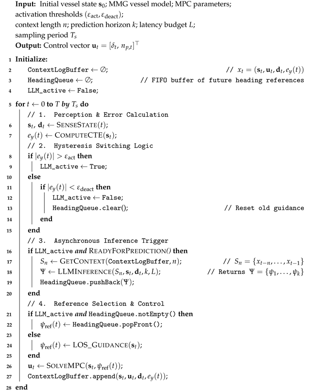
In an LLM-based guidance loop, the likelihood term can be interpreted as an implicit reweighting mechanism that amplifies the influence of those latent hypotheses that best explain the recent navigation context . Importantly, neither nor is explicitly estimated in the implementation, and no additional probabilistic inference or optimization is introduced. Operationally, this interpretation corresponds to Algorithm 1, where the LLM directly maps the serialized context window to a predictive heading sequence, which is subsequently filtered for feasibility and tracked by the MPC. Accordingly, the probabilistic expressions in this subsection should be interpreted as describing the implicit behavior of prompt-conditioned inference, rather than as quantities computed during execution.
Consider a case where a vessel navigates with LLM-based guidance under rough disturbances, and assume two hypothetical environment concepts: and . If recent contexts are collected under a rough condition, then
Because the guidance model uses the likelihood ratio in Equation (31), the rough model receives a much larger weight:
As a result, even though the LLM’s parameters are not updated, the LLM implicitly shifts its reasoning toward disturbance-aware behavior.
| Algorithm 1: LLM-Based Predictive–Adaptive Guidance with Inference |
 |
We map this probabilistic view (Equations (27)–(31)) to an interpretable three-stage CoT procedure, ensuring continuity and operational safety (Equations (32) and (33)):
- 1.
- Interpretation stage forms an implicit latent context by analyzing temporal correlations in and the current query (Equation (27));
- 2.
- Adjustment stage produces with the appropriate direction and magnitude to preempt drift (Equation (28));
- 3.
- Feasibility check stage enforces dynamic feasibility with respect to the vessel’s motion via heading-rate and path-deviation limits:
In summary, ICL supplies an adaptive prompt-conditioned substrate that can be interpreted through a Bayesian lens, while CoT imposes an interpretable three-stage procedure that respects continuity and operational safety constraints.
4.3. CoT-ICL Prompt Pipeline Design
In our formulation, CoT serves as the top-level reasoning scaffold, while ICL provides the contextual substrate upon which the reasoning is executed. This section operationalizes this probabilistic theory by detailing how the ICL–CoT mechanism is instantiated through state serialization, prompt composition, example curation, and output validation so that the LLM’s predictive headings can be executed reliably within the MPC loop.
We designed a CoT–ICL prompt pipeline to operate stably and with low-variance outputs under fixed generation settings, and safely in real-time settings, all without requiring any parameter updates. Figure 4 illustrates our CoT-ICL prompt pipeline.
Figure 4.
CoT–ICL prompt pipeline. Navigation history is serialized into a structured prompt, enabling the LLM to generate a k-step predictive heading sequence, which is then clipped for dynamic feasibility before MPC tracking.
At each guidance step t, the navigation data are serialized into the structured tuple defined in Equation (25) and accumulated within the sliding context window of Equation (26).
This window serves as the ICL memory, providing the LLM with a compact yet information-rich temporal context. The prompt is then assembled around a top-level CoT reasoning framework, which dictates how the LLM interprets this context and generates a disturbance-aware future heading sequence. Within this design, all subsequent prompt elements—preamble, in-context exemplars, and serialized state—are interpreted through the CoT scaffold. The CoT framework enforces the three-stage reasoning procedure formalized in Section 4.2.
This prompt design also clarifies why a general-purpose LLM can effectively operate on numerical navigation data. Although the LLM is trained on general text, it fundamentally operates on token sequences and can process structured numerical tokens when they are presented with consistent formatting and explicit semantics. In our framework, navigation data are not provided as raw untyped numbers; instead, they are serialized together with variable names, units, and a fixed temporal order, and the prompt specifies the intended output schema (a k-step heading reference sequence). Under this setup, the LLM primarily follows the prompt instructions and completes patterns in recent temporal trends (e.g., cross-track error evolution and drift direction) rather than relying on maritime-specific hydrodynamic knowledge, while physical validity and safety are ensured downstream by feasibility checks and MPC tracking.
- 1.
- Interpretation stage quantifies cross-track deviation, analyzes recent disturbance trends in , , , , and summarizes short-term motion patterns.
- 2.
- Adjustment stage determines the direction and relative magnitude of heading correction
- 3.
- Feasibility Check stage ensures that the proposed sequence satisfies the continuity and deviation limits. This high-level structure unifies all reasoning steps and makes the LLM’s predictions more interpretable and physically grounded.
CoT Reasoning Template in Figure 4 constructs the LLM prompt with the serialized inputs drawn from the Context Log Buffer, producing a coherent prompt for downstream inference. The CoT Reasoning Template is composed of two components: System Preamble and Few-Shot ICL Exemplars, as illustrated in Listing 1.
| Listing 1. LLM system prompt template. |
| You are an expert maritime guidance module supporting an MPC-based autopilot for a displacement-type tanker (KVLCC2 class). Your task is to generate a short-horizon sequence of heading references that is feasible for real-time tracking. |
| [SYSTEM PARAMETERS] - Prediction horizon: k steps (each step approx. 1 s). - Vessel characteristics: large inertia and slow turning response. - Maximum practical turn rate: approx. 5 deg/s. - Guidance update interval: 1.0 s. |
| [INPUT] You receive a context window S_n containing the last n time steps (t-n, …, t-1). Each entry includes: - Vessel states s = [x, y, psi, u, v, r], - Control inputs u = [delta, n_p], - Disturbance estimates d = [V_w, psi_w, V_c, psi_c], - Cross-track error CTE relative to the desired path. The current desired path bearing psi_path(t) is also provided. |
| [OBJECTIVE] Generate a sequence of k future heading references: Psi_{t:t+k-1} = [psi_1, psi_2, …, psi_k]. |
| [CHAIN-OF-THOUGHT REASONING] Before producing the sequence, briefly analyze: 1. Whether CTE is increasing, decreasing, or oscillating. 2. The direction and approximate influence of disturbances. 3. The magnitude of correction required to return toward the corridor centerline. |
| [OUTPUT FORMAT] Return a JSON object: { “reasoning”: “Short explanation of how the headings were chosen.”, “headings”: [psi_1, psi_2, …, psi_k] } |
The system preamble specifies the high-level task: given a serialized context window of recent navigation history, the LLM must generate a k-step sequence of future heading references that is smooth, physically plausible, and directly usable by the downstream MPC controller for real-time execution.
By explicitly stating this instruction, System preamble enforces unit consistency and ensures that the generated heading sequence remains compatible with the downstream dynamic-feasibility constraints of the control loop.
Few-shot ICL exemplars provide the LLM with small in-context demonstrations that illustrate the expected reasoning pattern and output structure. Our Few-Shot ICL Exemplars include three representative situations—minor deviation, severe deviation, and stabilization—each containing a brief history slice extracted from current sliding context window, a compact CoT rationale aligned with the scaffold above, and a target heading sequence. These exemplars draw on the benefits of CoT for multi-step reasoning and the effectiveness of lightweight zero-shot CoT prompting. (Wei et al. [36]; Kojima et al. [37]; Kothapalli et al. [42]).
System preamble provides a concise task description that anchors the LLM’s generation process and clarifies the expected output format.
4.4. Temporal Inference for Latency Compensation
Large Language Models (LLMs) inherently operate at a slower time resolution than real-time control loops due to their autoregressive decoding and multi-layer attention computation. The GPT-4 Technical Report (OpenAI et al. [43]) notes that such decoding latency “is non-negligible” and often ranges from several hundred milliseconds to multiple seconds, while Li et al. [44] emphasize that “real-time decision-making remains an open challenge due to inference time variability.” In a closed-loop guidance system, this latency does more than delay a response—it can create timing mismatches, interrupt heading—command updates, and degrade trajectory-tracking stability if the controller must wait for the LLM to finish computing.
To mitigate these latency-induced issues, the proposed guidance system introduces a Temporal Inference Framework that decouples the LLM’s inference cycle from the MPC’s synchronous control cycle. Figure 5 illustrates the underlying time-domain structure: once LLM activation occurs, three sliding windows operate in parallel: (i) a Context Window of length n, containing the most recent navigation history supplied to the LLM, (ii) an LLM Prediction Window, whose duration corresponds to the inference latency L and (iii) an MPC Execution Window of length k during which MPC executes the previously predicted heading sequence. These windows move forward together along the time axis, ensuring that the control loop remains continuous even while the LLM is still computing. Importantly, a smaller inference latency L allows the LLM to base its prediction on more recent log data, thereby improving responsiveness and reducing the risk of outdated contextual inference.
Figure 5.
Temporal inference framework decoupling LLM inference from real-time MPC control. Sliding context, prediction, and execution windows ensure continuous availability of heading commands despite LLM latency.
Formally, at time t, the LLM receives the most recent n-step navigation history, forming the context window
where includes vessel positions, velocities, heading, rudder angle, propeller speed, CTE, and disturbance information at time t. While the LLM processes this window, requiring L seconds, the MPC is not idle; instead, it continues to solve the tracking problem at every sampling instant using the remaining reference headings stored in the buffer. In this way, the vessel receives continuous and dynamically feasible control updates even while the LLM is computing the next heading sequence.
Once the LLM completes its computation, it outputs a predicted k-step future heading sequence
which becomes the reference trajectory for the next MPC cycle. Because the inference latency is L, the LLM effectively operates on a delayed context segment, producing
meaning the LLM predicts the future heading sequence based on the most recent navigation history available L seconds earlier. This temporal shift is the key to the sliding structure in Figure 5.
As the control loop progresses, the three windows slide forward in increments of k. At each iteration, the relationship between the context segment, the LLM prediction, and the MPC execution is described by the sliding sequence visualized in Figure 5.
- the LLM receives the context
- LLM generates the next predicted heading sequence
- and MPC executes this predicted segment
These expressions compactly represent the temporal shift shown by the blue (context), green (prediction), and red (MPC execution) arrows in Figure 5. Across iterations, the LLM functions as an asynchronous high-level predictor while the MPC performs synchronous real-time control, forming a rolling-horizon predictive–control loop.
The newly generated heading sequence is stored in an MPC buffer, ensuring that a continuous sequence of heading commands is always available. As the MPC consumes this sequence, the remaining inputs—along with updated disturbances—are added to the navigation log, forming the next context window for subsequent inference. This buffer mechanism guarantees smooth command delivery and preserves control continuity even when inference latency varies.
By combining asynchronous LLM inference with synchronous MPC execution, the proposed Temporal Inference Framework provides two crucial benefits:
- Continuous and stable control commands, maintained even when inference latency is non-negligible
- Real-time adaptivity, as the LLM continuously refreshes future heading predictions using the most recent available context.
Overall, this latency-aware predictive framework compensates for the computational delays inherent to large-scale LLMs and enables robust, real-time trajectory tracking in dynamic and uncertain maritime environments.
To consolidate the operational logic described in Section 4.1 and Section 4.4, Algorithm 1 presents the complete execution flow of our proposed LLM-based Predictive–Adaptive Guidance Framework. Our algorithm integrates three core components:
- Hysteresis-based switching rule activates or deactivates the LLM according to the vessel’s cross-track error,
- CoT-based LLM reasoning module generates a k-step sequence of predictive heading references, and
- Asynchronous temporal-inference mechanism supplies heading commands to the MPC despite non-negligible LLM latency.
Algorithm 1 illustrates how the guidance system smoothly transitions between conventional LOS guidance and LLM-driven predictive control. When the LLM is active, its predicted heading sequence is stored in a queue and consumed one step at a time by the MPC, while new predictions are generated asynchronously using the latest navigation context. When the LLM is inactive, the system automatically reverts to LOS-based reference generation.
This alternating flow ensures that the MPC always receives a valid reference heading—either reactive (LOS) or predictive (LLM)—thereby maintaining real-time continuity, robustness against disturbances, and stable closed-loop behavior. Algorithm 1 thus clarifies how the LLM reasoning layer, the temporal inference structure, and the MPC controller cooperate within a unified, latency-aware guidance architecture.
5. Simulation and Result Analysis
5.1. Simulation Environment Setup
Numerical simulations were performed using the scaled model of the KRISO Very Large Crude Carrier 2 (KVLCC2-L64, scale ratio 1:5) as the reference vessel. The ship hydrodynamics were modeled using the Maneuvering Modeling Group (MMG) formulation [29], and the corresponding coefficients were validated against the benchmark data published through the SIMMAN 2008 Workshop on Verification and Validation of Ship Manoeuvring Simulation Methods [45,46]. A predefined MMG-based KVLCC2-L64 configuration was employed, containing all principal geometric and hydrodynamic parameters required for the simulations. The main dimensions of the vessel model are summarized in Table 1.
Table 1.
Principal dimensions of the KVLCC2-L64 model (scale ratio 1:5).
The vessel was required to follow a predefined reference path while remaining within a tracking corridor. The corridor half-width was set to , providing an allowable deviation band of consistent with the KVLCC2-L64 maneuvering envelope. Two hysteresis thresholds regulated LLM activation: an activation threshold of and a deactivation threshold of , preventing chattering during mode switching.
The LOS look-ahead distance was set to , reflecting the vessel scale and expected disturbance magnitude. The heading-rate limit was chosen as per guidance step, and the allowable path-deviation angle was constrained to . These values fall within typical ranges reported in LOS–MPC and ILOS-based marine guidance literature.
Environmental disturbances consisted of a steady wind with speed and a uniform current with speed . Disturbance directions were selected from , representing quartering and bow-quartering conditions used across all scenarios. Although the global disturbance directions are fixed, the rectangular trajectory (structured as east–north–west–south legs) naturally exposes the vessel to a wide range of relative disturbance angles. As the heading rotates through all four cardinal directions, the same external disturbance is effectively encountered from multiple quadrants, providing representative coverage of diverse disturbance–heading configurations without explicitly varying the environmental direction.
The MPC controller operated at a sampling period of with a prediction horizon of and a control horizon of . Quadratic penalties were applied to minimize cross-track error and heading deviation while regularizing control effort. Rudder angle and propeller speed were constrained within physically meaningful limits consistent with the maneuvering characteristics of the KVLCC2-L64 model.
The LLM environment used Qwen2.5–Instruct (7B) with temperature and top- to promote deterministic reasoning. The Qwen2.5–Instruct (7B) model was selected as a compact LLM, providing sufficient capacity for structured CoT-based heading generation, while remaining compatible with practical onboard computational constraints [47]. In this context, the 7B scale represents a balanced design point, offering adequate reasoning capability without the latency and resource overhead associated with larger models.
To justify this choice for closed-loop operation, we provide a limited decoding-parameter sensitivity analysis and output-level reliability results in Section 5.3. In addition, a sensitivity analysis of the LOS–LLM switching thresholds (, ) is presented in Section 5.3 to assess the robustness of the proposed switching logic with respect to reasonable parameter variations. Simulations were executed on an NVIDIA RTX 4070 Ti GPU running CUDA 12.6.
To determine the latency budget L required for real-time operation, we measured the end-to-end LLM inference delay across combinations of context-window length n and prediction horizon k. Figure 6 reports the maximum observed latency for each pair, as closed-loop feasibility is dictated by worst-case timing rather than average performance. The largest delay was at . Accordingly, we set a conservative latency budget of to guarantee that the MPC always receives valid heading references even when the LLM operates at its slowest. Because latency depends on hardware and model configuration, L should be re-profiled when deploying to different platforms. All fixed simulation parameters are listed in Table 2. Together, this simulation environment provides a realistic platform for evaluating the proposed LLM-based Predictive–Adaptive Guidance Framework under nonlinear ship dynamics and disturbance-rich maritime operating conditions.
Figure 6.
Maximum end-to-end LLM inference latency over configurations. The worst-case delay ( at , ) motivates selecting a conservative latency budget of , ensuring that MPC always receives valid heading references despite asynchronous LLM computation.
Table 2.
Fixed simulation parameters used in all experiments.
5.2. Performance Evaluation Metrics
To quantitatively evaluate the effectiveness of the proposed LLM-based Predictive–Adaptive Guidance Framework, four core performance metrics were selected to characterize the vessel’s accuracy, safety, responsiveness, and control efficiency.
5.2.1. Root Mean Square Cross-Track Error (RMS CTE) [m]
RMS CTE quantifies overall trajectory-tracking accuracy by penalizing large deviations more heavily through squaring. A lower value indicates smoother and more precise path following, which is especially critical in constrained waterways or harbor-approach scenarios.
Here, N is the total number of simulation steps, and denotes the instantaneous cross-track error at time .
5.2.2. Corridor Compliance Rate (CCR) [%]
CCR measures the percentage of time the vessel remains within the allowable tracking corridor. Higher CCR values indicate stronger lateral containment, which is essential for safe passage in narrow channels and harbor entrances.
where N is the total number of simulation steps, is the corridor half-width (band ), and denotes the indicator function that returns 1 when the condition is satisfied and 0 otherwise.
5.2.3. Average Recovery Time [s]
This metric evaluates transient responsiveness by measuring how quickly the vessel returns to stable path following after a disturbance-induced excursion. Smaller values indicate faster disturbance rejection and improved maneuvering agility.
Here, M is the number of excursion events. The event start time is the first instant when exceeds the activation threshold . The recovery time is the first instant after when falls below the deactivation threshold . Excursions that do not recover within the simulation horizon are excluded from M.
5.2.4. Mean Absolute Rudder Angle (MARA) [°]
MARA represents the average magnitude of rudder deflection required to maintain trajectory tracking. It serves as a practical proxy for steering effort and actuator workload.
where is the rudder angle at time . Note that MARA does not capture oscillatory behavior or high-frequency variations in rudder motion; therefore, it is interpreted conservatively as an effort-related metric.
5.2.5. LLM Output Reliability Metrics
In addition to trajectory-level metrics, we quantify the output-level reliability of the LLM in closed-loop operation. The valid-output rate measures the fraction of LLM inference calls that return a JSON-parsable numeric heading sequence of length k:
The clipping activation rate measures how often the raw LLM heading violates the continuity and deviation limits in Equations (34) and (35):
These indicators complement RMS CTE, CCR, , and MARA by assessing whether the generated heading references are stable and executable beyond final tracking accuracy. In Section 5.3, these metrics are used to compare the proposed LLM–MPC framework with the baseline LOS–MPC controller and to analyze performance differences under varying disturbance conditions.
5.3. Simulation Results and Analysis
5.3.1. Scenario Design and Experimental Setup
To evaluate both performance gains and practical tuning characteristics, four scenarios were constructed as summarized in Table 3. Scenarios 1 and 2 focus on effectiveness (baseline guidance vs. LLM-augmented guidance) under two disturbance directions ( and ). Scenarios 3 and 4 provide ablation insight on temporal parameters of the LLM module, i.e., the context-window length n and prediction horizon k, under a fixed disturbance for controlled comparison. In all scenarios, LLM reasoning is invoked only when the cross-track error (CTE) exceeds the activation threshold (yellow segments in the trajectory plots), thereby testing the intended selective use of inference rather than continuous replanning.
Table 3.
Summary of simulation scenarios and parameter configurations. All scenarios assume a disturbance environment of and . For baseline cases without LLM assistance, n and k are not applicable (“–”).
- Scenario 1:
- Assesses whether the proposed LOS + LLM + MPC architecture improves robustness and corridor tracking compared with the baseline LOS + MPC loop under strong quartering and bow-quartering disturbances.
- Scenario 2:
- Examines whether the LLM layer remains beneficial when combined with Integral LOS (ILOS), which already includes drift-rejection via an integral term. This scenario specifically targets cases where large CTE excursions still occur under strong disturbances, testing whether predictive, context-aware heading references can accelerate recovery beyond what integral compensation alone provides.
- Scenario 3:
- Studies how the temporal memory length () affects the stability and consistency of the LLM’s predictive corrections with a fixed prediction horizon .
- Scenario 4:
- Analyzes how the horizon length () influences responsiveness and oscillatory behavior when the context window is fixed at .
Overall, this design enables a component-wise validation of performance improvements (Scenarios 1 and 2) and yields actionable guidelines for choosing in latency- and stability-sensitive deployments (Scenarios 3 and 4).
5.3.2. Scenario 1—LOS Guidance Under Disturbances
Scenario 1 compares the baseline LOS + MPC controller (Case 1) with the proposed LOS + LLM + MPC framework (Case 2, , ) under two disturbance directions ( and ). The trajectories in Figure 7 show that LLM activation (yellow) occurs primarily during large deviations, after which the vessel re-enters the corridor and continues tracking under nominal LOS guidance.
Figure 7.
Path–tracking trajectories for Scenario 1 under LOS guidance with (left) and (right) disturbances. Yellow segments indicate LLM activation.
Quantitative comparisons in Figure 8 confirm consistent improvements in tracking accuracy and recovery. Under the disturbance, RMS CTE decreases from 28.63 m to 24.18 m (a 15.5% reduction), corridor compliance increases from 79.12% to 83.74% (+4.62 percentage points), and recovery time shortens from 168.50 s to 136.00 s (a 19.3% reduction). Under the disturbance, the same trend holds: RMS CTE improves from 25.78 m to 23.74 m (7.9% reduction), corridor compliance rises from 80.20% to 83.88% (+3.68 percentage points), and recovery time decreases from 159.00 s to 137.00 s (13.8% reduction). Importantly, mean absolute rudder usage remains almost unchanged in both cases (13.95° → 14.02° at 225°, and 13.66° → 13.69° at 45°), indicating that the improved robustness is achieved without materially increasing steering effort. These results support the central claim of Scenario 1: embedding selective, short-horizon LLM-based prediction within the guidance loop yields tighter path keeping, higher corridor containment, and faster disturbance recovery across disturbance directions, while maintaining comparable actuator workload.
Figure 8.
Quantitative performance metrics for Scenario 1 under LOS guidance with (top) and (bottom) disturbances.
5.3.3. Scenario 2—ILOS Guidance Under Disturbances
Scenario 2 evaluates whether the LLM layer remains effective when paired with ILOS guidance, which already improves drift rejection through an integral correction term. In this study, the ILOS integral parameters were set to an integral gain of 0.05 with an integral saturation limit of 100. Case 1 is the baseline ILOS + MPC controller, and Case 2 is the proposed ILOS + LLM + MPC framework with . As shown in Figure 9, LLM activation again occurs selectively during large deviations, suggesting that the proposed module is not used as a constant “planner” but as an on-demand predictor for disturbance-driven excursions.
Figure 9.
Path–tracking trajectories for Scenario 2 under ILOS guidance with (left) and (right) disturbances. Yellow segments indicate LLM activation.
Figure 10 shows that LLM augmentation yields substantial gains even on top of ILOS. Under the disturbance, RMS CTE drops from 27.90 m to 15.16 m (45.6% reduction), corridor compliance rises from 81.65% to 94.49% (+12.84 percentage points), and recovery time shortens from 168.72 s to 77.00 s (54.4% reduction). Under the disturbance, RMS CTE decreases from 19.41 m to 12.44 m (35.9% reduction), corridor compliance increases from 88.34% to 96.14% (+7.80 percentage points), and recovery time improves from 96.69 s to 60.00 s (37.9% reduction). In contrast to Scenario 1, mean absolute rudder usage decreases slightly in both cases (10.76° → 10.38° at 225°, and 10.87° → 10.43° at 45°), implying that the improved recovery is not achieved through higher steering effort, but through better-aligned predictive heading references.
Figure 10.
Quantitative performance metrics for Scenario 2 (ILOS) under (top) and (bottom) disturbances.
Overall, Scenario 2 indicates that the LLM-based predictive heading layer complements (rather than duplicates) the integral drift compensation of ILOS: it provides anticipatory, context-aware corrections during excursions, leading to markedly faster recovery and stronger corridor containment under strong disturbances.
5.3.4. Scenario 3—Effect of Context Window Length (n)
Scenario 3 investigates how the LLM’s temporal context length affects predictive correction under LOS guidance for a fixed disturbance. Figure 11 (left) compares trajectories for (Case 1), (Case 2), and (Case 3), with fixed. While all cases eventually remain within the corridor, their transient behavior differs: a very short context can be insufficient for reliable trend inference, whereas an overly long context may introduce stale historical patterns that no longer match the current disturbance–response regime, increasing oscillatory corrections.
Figure 11.
Trajectory comparison for Scenario 3 (left, different context-window sizes) and Scenario 4 (right, varying prediction horizons) under LOS guidance with disturbances.
The quantitative outcomes in Figure 12 reflect this trade-off. Case 2 () achieves the lowest RMS CTE (23.76 m) and the lowest mean absolute rudder usage (13.81°), indicating the most efficient and stable correction among the tested settings. Corridor compliance for remains high (84.18%) and is essentially comparable to the short-window case (84.32% at ), while recovery times are also similar for and (133.50 s vs. 132.50 s). In contrast, Case 3 () exhibits a much shorter recovery time (86.00 s) but at the cost of increased oscillation and substantially higher steering effort (16.29°) as well as reduced corridor compliance (82.75%). This indicates that the apparent “fast recovery” at is largely driven by aggressive corrective swings, which is undesirable for smooth and energy-efficient maneuvering.
Figure 12.
Scenario 3: quantitative ablation across context-window lengths. Yellow labels denote relative improvement with respect to the metric-wise mean (positive is better).
In summary, Scenario 3 suggests that excessively long context windows can dilute the LLM’s inference with outdated history and promote oscillatory corrections, whereas a moderate context length () provides the best balance between accuracy, stability, and steering efficiency under persistent disturbances.
5.3.5. Scenario 4—Effect of Prediction Horizon (k)
Scenario 4 examines how the LLM’s prediction horizon influences closed-loop behavior when the context window is fixed at . Figure 11 (right) illustrates that shorter horizons support more frequent refresh of corrective heading references, while longer horizons reduce update frequency and can accumulate prediction drift under persistent disturbances, potentially inducing zigzagging motion.
Figure 13 shows a consistent trend. Case 1 () achieves the lowest RMS CTE (22.11 m) and the highest corridor compliance (85.18%), indicating the most centered and stable tracking. Case 2 () yields nearly identical accuracy (22.20 m) with slightly lower corridor compliance (84.87%) and comparable recovery time (126.00 s), while achieving the lowest mean absolute rudder usage among the tested horizons (13.64°). Case 3 () produces the shortest recovery time (106.00 s) but clearly at the cost of reduced corridor compliance (82.09%) and significantly higher steering demand (15.50°), which is consistent with the visibly more oscillatory trajectory. Thus, the shorter recovery time for long horizons should be interpreted as a byproduct of stronger corrective swings rather than improved stability or efficiency.
Figure 13.
Scenario 4: ablation across prediction horizons. Yellow labels denote relative improvement with respect to the metric-wise mean (positive is better).
Taken together with Scenario 3, these results suggest that practical deployment should prefer moderate context lengths and short horizons; in our experiments, provides the best overall balance among tracking accuracy, corridor containment, responsiveness, and steering effort, while avoiding oscillatory behavior associated with overly long temporal settings.
5.3.6. Sensitivity Analysis of Key Design Parameters
This subsection examines the sensitivity of the proposed LOS–LLM–MPC framework to practical design parameters. We study (i) the effect of LLM decoding settings on closed-loop tracking performance and output executability, and (ii) the robustness of the hysteresis-based LOS–LLM switching thresholds that govern mode transitions. The intent is not to claim a single optimal setting, but to identify a stable operating region in which the proposed framework maintains consistent performance and reliable LLM outputs within reasonable parameter ranges.
We first analyze the influence of LLM decoding parameters on closed-loop behavior. The decoding temperature and nucleus sampling threshold affect the variability of the generated heading references, which in turn influences tracking accuracy, responsiveness, and output executability. Table 4 reports trajectory-level performance metrics together with output-level reliability indicators under the Scenario 1 test conditions.
Table 4.
Decoding parameter sensitivity and output-level reliability (Scenario 1, disturbance; , ). The baseline corresponds to the LOS–MPC controller without LLM assistance.
Compared to the baseline LOS–MPC controller, all LLM-assisted configurations yield substantial improvements in RMS CTE and corridor compliance, indicating consistent benefits without requiring precise tuning. At very low decoding temperatures (), the generated references are highly stable and clipping is rarely triggered, but the guidance can become conservative under strong disturbances. As decoding randomness increases ( with a higher top-p), the LLM tends to react more aggressively, which can shorten recovery time but also increases output variability; this is reflected by a lower valid-output rate (i.e., more frequent JSON-parsing failures) and more frequent feasibility filtering. Overall, operating in a practical low-temperature regime (e.g., ) provides a well-balanced behavior, achieving strong tracking performance while maintaining stable, JSON-parsable outputs without fine-grained parameter tuning.
We next evaluate the sensitivity of the hysteresis-based LOS–LLM switching logic, which determines when the LLM-assisted guidance is engaged. The LLM is activated when the cross-track error satisfies and is deactivated once ; the hysteresis gap () is used to prevent frequent mode toggling. In the nominal configuration, we set and , using a fixed ratio . To assess robustness to coarse threshold selection (rather than precise tuning), we vary within a range while preserving the same hysteresis ratio, and report both tracking metrics and switching statistics (LLM active ratio and number of mode transitions) in Table 5.
Table 5.
Sensitivity of the LOS–LLM switching thresholds (, ) under Scenario 1 ( disturbance). The deactivation threshold is fixed to to preserve the hysteresis structure of the switching logic. Here, Active denotes the percentage of time steps during which the LLM is active, and Switches is the number of LOS–LLM mode transitions.
The results in Table 5 indicate that the overall closed-loop tracking performance remains consistent across the tested threshold values, while the thresholds primarily affect how often (and how early) the LLM-assisted mode is invoked. Lower thresholds increase the LLM active ratio and switching count, whereas higher thresholds reduce LLM usage and delay its engagement; importantly, these changes do not lead to qualitative performance degradation. This suggests that the switching logic maintains stable behavior within a reasonable range and does not depend on finely tuned threshold values.
Overall, the results support that the proposed LOS–LLM–MPC framework admits a stable operating region with respect to both decoding parameters and switching thresholds: reasonable low-variance decoding settings yield reliable, executable outputs, and the hysteresis thresholds can be selected coarsely without undermining closed-loop tracking performance.
6. Conclusions
We presented an LLM-based Predictive–Adaptive Guidance Framework that integrates a Large Language Model directly within the closed-loop control architecture of an autonomous surface vessel. By allowing the LLM to interpret navigation history, infer disturbance trends, and generate future heading references in real time, the proposed framework moves beyond the conventional use of LLMs as high-level decision-support tools and demonstrates their feasibility as context-aware anticipatory reference-generation modules embedded within physical control systems. Through In-Context Learning and Chain-of-Thought reasoning, the LLM adapts its outputs based solely on contextual information—without parameter updates—while a latency-aware temporal inference structure harmonizes asynchronous LLM computation with synchronous MPC execution, preserving control continuity under non-negligible inference delays.
Extensive simulations using the MMG-based KVLCC2-L64 model under wind and current disturbances showed that the proposed LLM–MPC architecture consistently outperforms a representative LOS–MPC controller. It achieved tighter path keeping, higher corridor compliance, and faster disturbance recovery, while maintaining comparable steering effort despite operating with a frozen-parameter LLM. These results provide strong evidence that LLM-based contextual reasoning can meaningfully contribute to real-time control when supported by proper temporal coordination and model-predictive execution.
Overall, this work suggests a promising direction toward knowledge-driven, context-aware, and adaptively predictive control architectures for autonomous maritime systems.
The evaluation in this study focuses on simulation-based scenarios with persistent wind and current disturbances, which provide a controlled and repeatable setting for analyzing LLM-assisted guidance under sustained disturbance-induced deviations. Within this scope, the reported results are intended to demonstrate the feasibility and effectiveness of the proposed framework as a proof-of-concept, rather than to fully characterize performance under rapidly varying stochastic effects such as wind gusts, irregular waves, or sensor noise.
Future research will extend the framework to time-varying and stochastic disturbance environments. In addition, validation using real-world onboard sensor data and hardware-in-the-loop experiments will be pursued to rigorously assess robustness and practical deployability.
Author Contributions
Conceptualization, S.L. and W.K.; methodology, S.L. and W.K.; software, S.L.; validation, S.L., Y.J. and W.K.; formal analysis, S.L.; investigation, W.K.; resources, S.L.; data curation, S.L. and Y.J.; writing—original draft preparation, S.L.; writing—review and editing, S.L. and W.K.; visualization, S.L. and Y.J.; supervision, W.K.; project administration, W.K.; funding acquisition, W.K. All authors have read and agreed to the published version of the manuscript.
Funding
This work was supported by IITP (Institute of Information and communications Technology Planning and Evaluation)-ICAN (ICT Challenge and Advanced Network of HRD) grant funded by the Korea government (Ministry of Science and ICT) (IITP-2024-00436744). This work was supported by the Dongguk University Research Fund of 2015.
Data Availability Statement
The simulation data and code used in this study are available from the corresponding author upon reasonable request. No publicly archived datasets were generated.
Conflicts of Interest
The authors declare no conflicts of interest. The funders had no role in the design of the study; in the collection, analyses, or interpretation of data; in the writing of the manuscript; or in the decision to publish the results.
Abbreviations
The following abbreviations are used in this manuscript:
| AI | Artificial Intelligence |
| ALOS | Adaptive Line-of-Sight |
| AMV | Autonomous Marine Vessel |
| AUV | Autonomous Underwater Vehicle |
| CCR | Corridor Compliance Rate |
| CoT | Chain-of-Thought |
| CLOS | Classical Line-of-Sight |
| CUDA | Compute Unified Device Architecture |
| CTE | Cross-Track Error |
| DOF | Degree of Freedom |
| ELOS | Extended Line-of-Sight |
| ESO | Extended State Observer |
| GPU | Graphics Processing Unit |
| HLOS-FPF | Hyperbolic-Tangent LOS-Based Finite-Time Path-Following |
| ICL | In-Context Learning |
| ILOS | Integral Line-of-Sight |
| KVLCC2 | KRISO Very Large Crude Carrier 2 |
| L64 | 1:5 scaled KVLCC2 model ( m) |
| LLM | Large Language Model |
| LOS | Line-of-Sight |
| Length Between Perpendiculars | |
| MARA | Mean Absolute Rudder Angle |
| MASS | Maritime Autonomous Surface Ship |
| MMG | Maneuvering Modeling Group |
| MPC | Model Predictive Control |
| RL | Reinforcement Learning |
| RMS | Root Mean Square |
| SIMMAN | Workshop on Verification and Validation of Ship Manoeuvring Simulation Methods |
| SMC | Sliding Mode Control |
| USV | Unmanned Surface Vessel |
References
- Bai, X.; Li, B.; Xu, X.; Xiao, Y. A Review of Current Research and Advances in Unmanned Surface Vehicles. J. Mar. Sci. Appl. 2022, 21, 47–58. [Google Scholar] [CrossRef] [Scilit]
- Boretti, A. Navigating the future: The expanding role of unmanned surface vehicles in maritime security. J. Transp. Secur. 2025, 18, 24. [Google Scholar] [CrossRef] [Scilit]
- Kim, J.; Han, S.; Lee, H.; Koo, B.; Nam, M.; Jang, K.; Lee, J.; Chung, M. Trend Research on Maritime Autonomous Surface Ships (MASSs) Based on Shipboard Electronics. Electronics 2024, 13, 1902. [Google Scholar] [CrossRef] [Scilit]
- Xu, H.; Guedes Soares, C. Review of Path-following Control Systems for Maritime Autonomous Surface Ships. J. Mar. Sci. Appl. 2023, 22, 153–171. [Google Scholar] [CrossRef] [Scilit]
- Fossen, T. Handbook of Marine Craft Hydrodynamics and Motion Control; Wiley: Hoboken, NJ, USA, 2011. [Google Scholar] [CrossRef] [Scilit]
- Fossen, T.; Breivik, M.; Skjetne, R. Line-of-sight path following of underactuated marine craft. In Proceedings of the IFAC Proceedings Volumes, Girona, Spain, 17–19 September 2003; pp. 211–216. [Google Scholar] [CrossRef] [Scilit]
- Gu, N.; Wang, D.; Peng, Z.; Wang, J.; Han, Q.L. Advances in Line-of-Sight Guidance for Path Following of Autonomous Marine Vehicles: An Overview. IEEE Trans. Syst. Man Cybern. Syst. 2023, 53, 12–28. [Google Scholar] [CrossRef] [Scilit]
- Qiao, Y.; Yin, J.; Wang, W.; Duarte, F.; Yang, J.; Ratti, C. Survey of Deep Learning for Autonomous Surface Vehicles in the Marine Environment. arXiv 2023, arXiv:2210.08487. [Google Scholar] [CrossRef] [Scilit]
- Wang, P.; Liu, R.; Tian, X.; Zhang, X.; Qiao, L.; Wang, Y. Obstacle avoidance for environmentally-driven USVs based on deep reinforcement learning in large-scale uncertain environments. Ocean Eng. 2023, 270, 113670. [Google Scholar] [CrossRef] [Scilit]
- Agyei, K.; Sarhadi, P.; Naeem, W. Large Language Model-based Decision-making for COLREGs and the Control of Autonomous Surface Vehicles. In Proceedings of the 2025 European Control Conference (ECC), Thessaloniki, Greece, 24–27 June 2025; pp. 1761–1766. [Google Scholar] [CrossRef] [Scilit]
- Miller, T.; Durlik, I.; Kostecka, E.; Łobodzińska, A.; Łazuga, K.; Kozlovska, P. Leveraging Large Language Models for Enhancing Safety in Maritime Operations. Appl. Sci. 2025, 15, 1666. [Google Scholar] [CrossRef] [Scilit]
- Yang, R.; Hou, M.; Wang, J.; Zhang, F. OceanChat: Piloting Autonomous Underwater Vehicles in Natural Language. arXiv 2023, arXiv:2309.16052. [Google Scholar] [CrossRef] [Scilit]
- Fossen, T. An Adaptive Line-of-Sight (ALOS) Guidance Law for Path Following of Aircraft and Marine Craft. IEEE Trans. Control Syst. Technol. 2023, 31, 2887–2894. [Google Scholar] [CrossRef] [Scilit]
- Li, Y.; Wan, J.; Wang, X.; Sun, Z.; Li, H.; Yu, Z.; Kou, L.; Li, J.; Yang, Y. Path-Following Control Based on ALOS Guidance Law for USV. Electronics 2025, 14, 749. [Google Scholar] [CrossRef] [Scilit]
- Liu, L.; Wang, D.; Peng, Z.; Wang, H. Predictor-based LOS guidance law for path following of underactuated marine surface vehicles with sideslip compensation. Ocean Eng. 2016, 124, 340–348. [Google Scholar] [CrossRef] [Scilit]
- Liu, L.; Wang, D.; Peng, Z. ESO-Based Line-of-Sight Guidance Law for Path Following of Underactuated Marine Surface Vehicles with Exact Sideslip Compensation. IEEE J. Ocean. Eng. 2017, 42, 477–487. [Google Scholar] [CrossRef] [Scilit]
- Yu, C.; Liu, C.; Lian, L.; Xiang, X.; Zeng, Z. ELOS-based path following control for underactuated surface vehicles with actuator dynamics. Ocean Eng. 2019, 187, 106139. [Google Scholar] [CrossRef] [Scilit]
- Wiig, M.; Pettersen, K.; Ruud, E.L.; Krogstad, T. An Integral Line-of-Sight Guidance Law with a Speed-dependent Lookahead Distance. In Proceedings of the European Control Conference, Limassol, Cyprus, 12–15 June 2018; pp. 1269–1276. [Google Scholar] [CrossRef] [Scilit]
- Wang, N.; Ahn, C. Hyperbolic-Tangent LOS Guidance-Based Finite-Time Path Following of Underactuated Marine Vehicles. IEEE Trans. Ind. Electron. 2020, 67, 8566–8575. [Google Scholar] [CrossRef] [Scilit]
- Caharija, W.; Pettersen, K.Y.; Bibuli, M.; Calado, P.; Zereik, E.; Braga, J.; Gravdahl, J.T.; Sørensen, A.J.; Milovanović, M.; Bruzzone, G. Integral Line-of-Sight Guidance and Control of Underactuated Marine Vehicles: Theory, Simulations, and Experiments. IEEE Trans. Control Syst. Technol. 2016, 24, 1623–1642. [Google Scholar] [CrossRef] [Scilit]
- Guo, W.; Liu, C.; Sun, T. Cooperative Maritime Search of Multi-Ship Based on Improved Robust Line-of-Sight Guidance. J. Mar. Sci. Eng. 2024, 12, 105. [Google Scholar] [CrossRef] [Scilit]
- Fan, Y.; Sun, Z.; Wang, G. A novel intelligent collision avoidance algorithm based on deep reinforcement learning approach for USV. Ocean Eng. 2023, 287, 115649. [Google Scholar] [CrossRef] [Scilit]
- Cui, Z.; Guan, W.; Zhang, X. USV formation navigation decision-making through hybrid deep reinforcement learning using self-attention mechanism. Expert Syst. Appl. 2024, 256, 124906. [Google Scholar] [CrossRef] [Scilit]
- Zhao, Y.; Ma, Y.; Hu, S. USV Formation and Path-Following Control via Deep Reinforcement Learning With Random Braking. IEEE Trans. Neural Netw. Learn. Syst. 2021, 32, 5468–5478. [Google Scholar] [CrossRef] [Scilit]
- Zhao, Y.; Qi, X.; Ma, Y.; Li, Z.; Malekian, R.; Sotelo, M.A. Path Following Optimization for an Underactuated USV Using Smoothly-Convergent Deep Reinforcement Learning. IEEE Trans. Intell. Transp. Syst. 2021, 22, 6208–6220. [Google Scholar] [CrossRef] [Scilit]
- Christensen, K.; Gusev, A.; Tufte, A.; Alsos, O.; Steinert, M. AI Captain: Conversational mission planning and execution system for autonomous surface vehicles. Ocean Eng. 2025, 338, 121988. [Google Scholar] [CrossRef] [Scilit]
- Pei, D.; He, J.; Liu, K.; Chen, M.; Zhang, S. Application of Large Language Models and Assessment of Their Ship-Handling Theory Knowledge and Skills for Connected Maritime Autonomous Surface Ships. Mathematics 2024, 12, 2381. [Google Scholar] [CrossRef] [Scilit]
- Yang, R.; Zhang, F.; Hou, M. OceanPlan: Hierarchical Planning and Replanning for Natural Language AUV Piloting. In Proceedings of the WUWNET ’24, Šibenik, Croatia, 28–31 October 2024; pp. 1–5. [Google Scholar] [CrossRef] [Scilit]
- Yasukawa, H.; Yoshimura, Y. Introduction of MMG standard method for ship maneuvering predictions. J. Mar. Sci. Technol. 2015, 20, 37–52. [Google Scholar] [CrossRef] [Scilit]
- Isherwood, R. Wind resistance of merchant ships. Trans. R. Inst. Nav. Archit. 1973, 115, 327–338. [Google Scholar]
- Mann, B.; Ryder, N.; Subbiah, M.; Kaplan, J.; Dhariwal, P.; Neelakantan, A.; Shyam, P.; Sastry, G.; Askell, A.; Agarwal, S. Language Models are Few-Shot Learners. arXiv 2020, arXiv:2005.14165. [Google Scholar] [CrossRef] [Scilit]
- Chen, Y.; Zhong, R.; Zha, S.; Karypis, G.; He, H. Meta-learning via Language Model In-context Tuning. arXiv 2022, arXiv:2110.07814. [Google Scholar] [CrossRef] [Scilit]
- Dai, D.; Sun, Y.; Dong, L.; Hao, Y.; Ma, S.; Sui, Z.; Wei, F. Why Can GPT Learn In-Context? Language Models Implicitly Perform Gradient Descent as Meta-Optimizers. arXiv 2023, arXiv:2212.10559. [Google Scholar] [CrossRef] [Scilit]
- Garg, S.; Tsipras, D.; Liang, P.; Valiant, G. What Can Transformers Learn In-Context? A Case Study of Simple Function Classes. In Proceedings of the 38th International Conference on Machine Learning (ICML), Virtual, 18–24 July 2021; pp. 3682–3691. [Google Scholar]
- Xie, S.; Raghunathan, A.; Liang, P.; Ma, T. An Explanation of In-context Learning as Implicit Bayesian Inference. arXiv 2022, arXiv:2111.02080. [Google Scholar] [CrossRef] [Scilit]
- Wei, J.; Wang, X.; Schuurmans, D.; Bosma, M.; Ichter, B.; Xia, F.; Chi, E.H.; Le, Q.V.; Zhou, D. Chain-of-Thought Prompting Elicits Reasoning in Large Language Models. Adv. Neural Inf. Process. Syst. 2022, 35, 24824–24837. [Google Scholar]
- Kojima, T.; Gu, S.; Reid, M.; Matsuo, Y.; Iwasawa, Y. Large Language Models are Zero-Shot Reasoners. arXiv 2023, arXiv:2205.11916. [Google Scholar] [CrossRef] [Scilit]
- Suzgun, M.; Scales, N.; Schärli, N.; Gehrmann, S.; Tay, Y.; Chung, H.W.; Chowdhery, A.; Le, Q.V.; Chi, E.H.; Zhou, D.; et al. Challenging BIG-Bench Tasks and Whether Chain-of-Thought Can Solve Them. arXiv 2022, arXiv:2210.09261. [Google Scholar]
- Wang, X.; Wei, J.; Schuurmans, D.; Le, Q.; Chi, E.; Narang, S.; Chowdhery, A.; Zhou, D. Self-Consistency Improves Chain of Thought Reasoning in Language Models. arXiv 2023, arXiv:2203.11171. [Google Scholar] [CrossRef] [Scilit]
- Wies, N.; Levine, Y.; Shashua, A. The Learnability of In-Context Learning. arXiv 2023, arXiv:2303.07895. [Google Scholar] [CrossRef] [Scilit]
- Wang, B.; Min, S.; Deng, X.; Shen, J.; Wu, Y.; Zettlemoyer, L.; Sun, H. Towards Understanding Chain-of-Thought Prompting: An Empirical Study of What Matters. In Proceedings of the ACL 2023, Toronto, ON, Canada, 9–14 July 2023; pp. 2717–2739. [Google Scholar] [CrossRef] [Scilit]
- Kothapalli, V.; Firooz, H.; Sanjabi, M. CoT-ICL Lab: A Synthetic Framework for Studying Chain-of-Thought Learning from In-Context Demonstrations. arXiv 2025, arXiv:2502.15132. [Google Scholar] [CrossRef] [Scilit]
- OpenAI; Achiam, J.; Adler, S.; Agarwal, S.; Ahmad, L.; Akkaya, I.; Aleman, F.L.; Almeida, D.; Altenschmidt, J.; Altman, S.; et al. GPT-4 Technical Report. arXiv 2024, arXiv:2303.08774. [Google Scholar] [CrossRef] [Scilit]
- Li, Y.; Li, Z.; Yang, W.; Liu, C. RT-LM: Uncertainty-Aware Resource Management for Real-Time Inference of Language Models. arXiv 2023, arXiv:2309.06619. [Google Scholar] [CrossRef] [Scilit]
- Stern, F.; Agdrup, K.; Kim, S.Y.; Cura Hochbaum, A.; Rhee, K.; Quadvlieg, F.; Perdon, P.; Hino, T.; Broglia, R.; Gorski, J. Experience from SIMMAN 2008—The First Workshop on Verification and Validation of Ship Manoeuvring Simulation Methods. J. Ship Res. 2011, 55, 135–147. [Google Scholar] [CrossRef] [Scilit]
- SIMMAN. Part C: Captive and Free Model Test Data. In Proceedings of the Workshop on Verification and Validation of Ship Manoeuvring Simulation Methods, Copenhagen, Denmark, 13–17 April 2008. [Google Scholar]
- Qwen Team. Qwen2.5 Technical Report. arXiv 2025, arXiv:2412.15115. [Google Scholar]
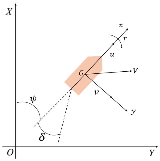
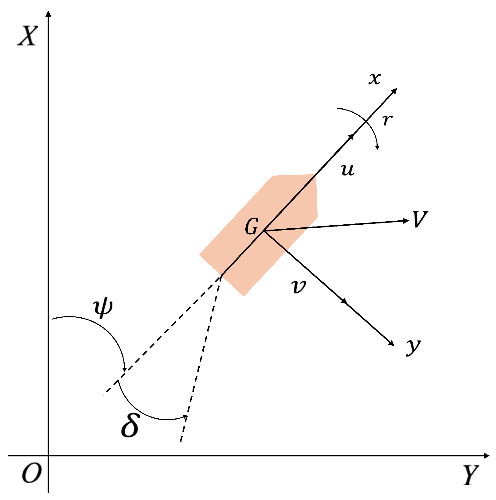
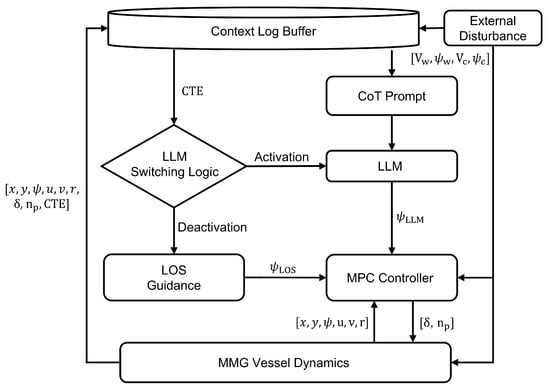
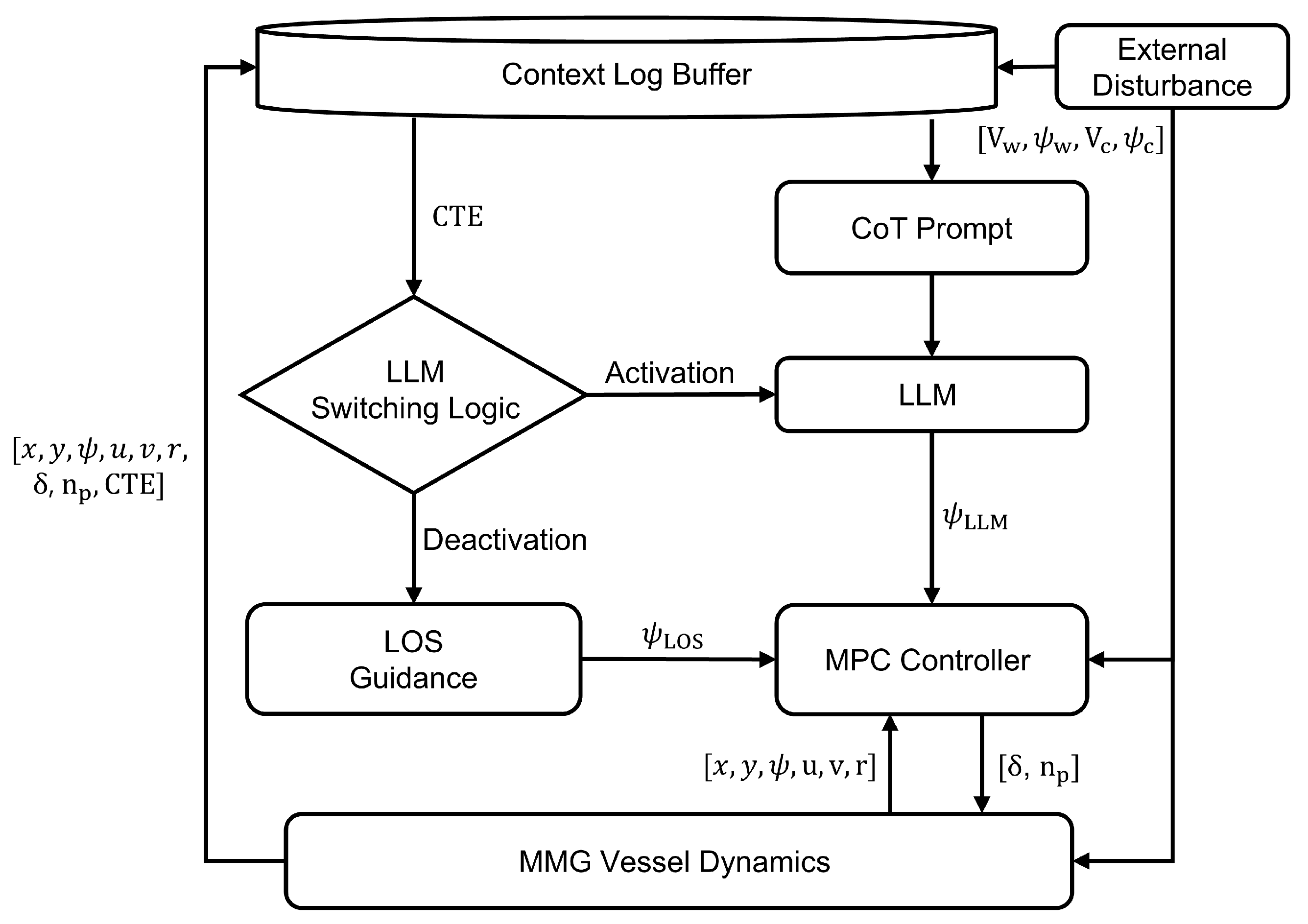
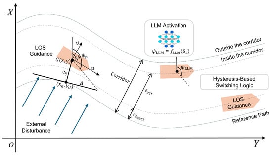
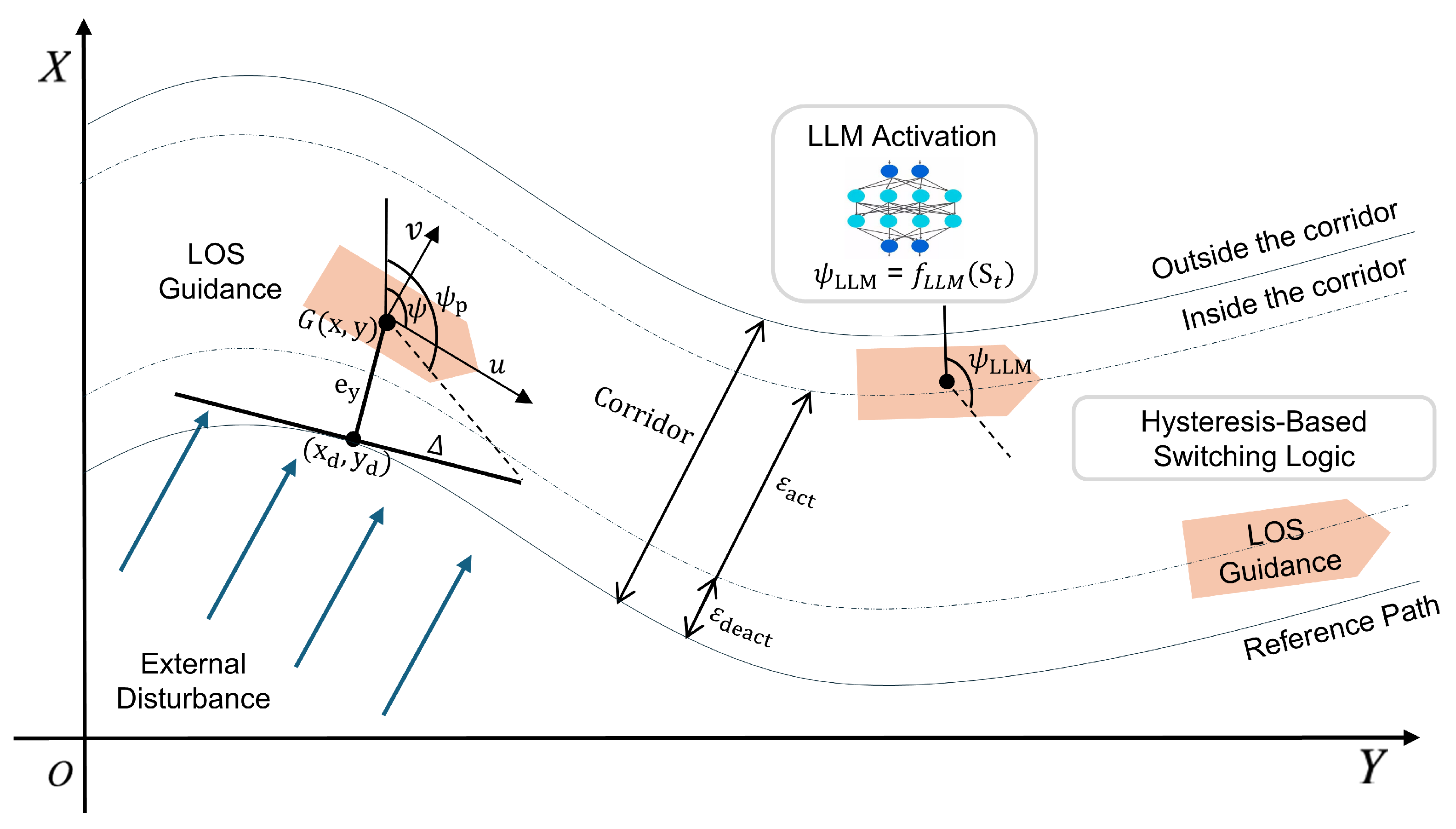


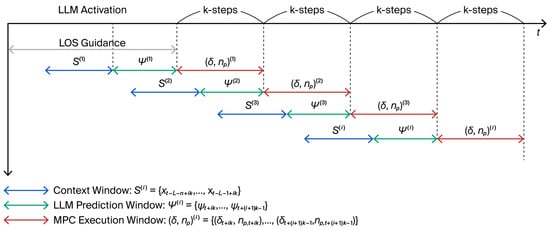
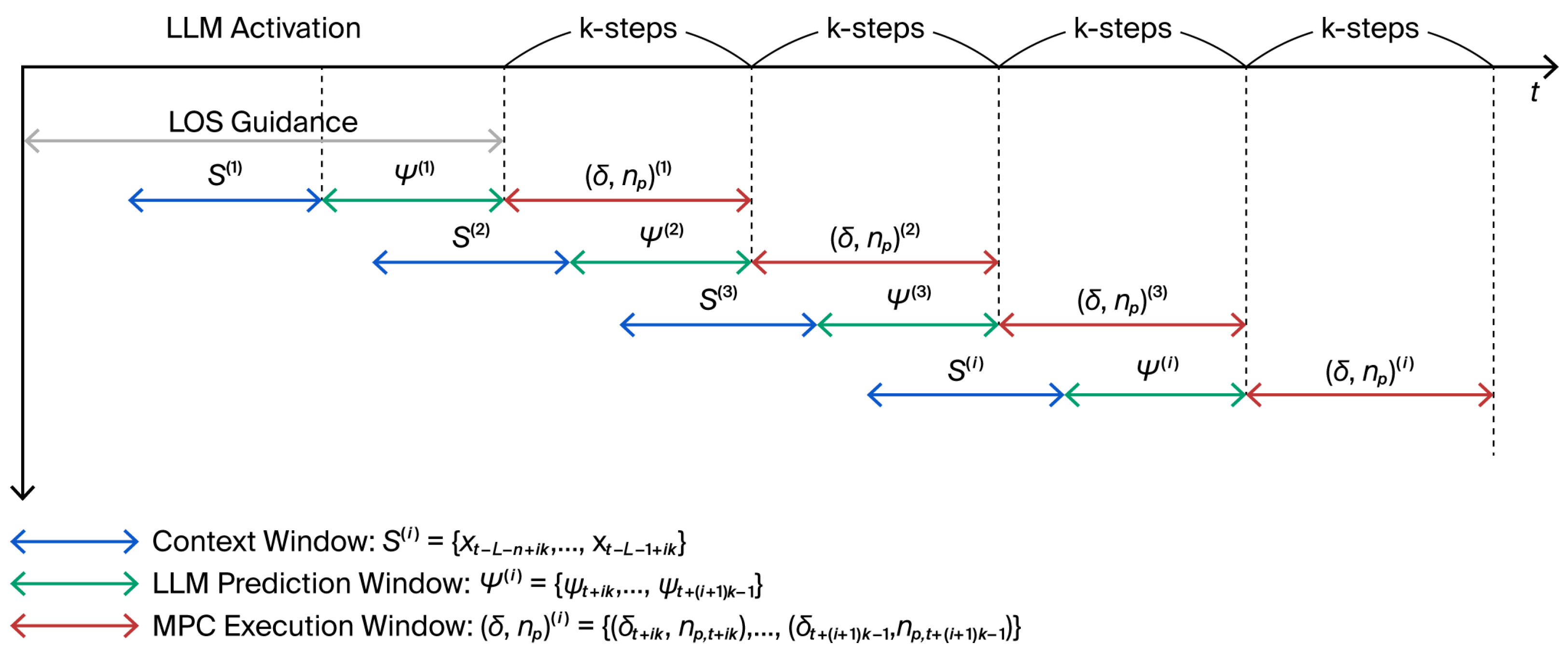
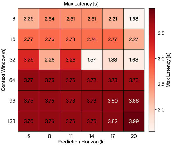
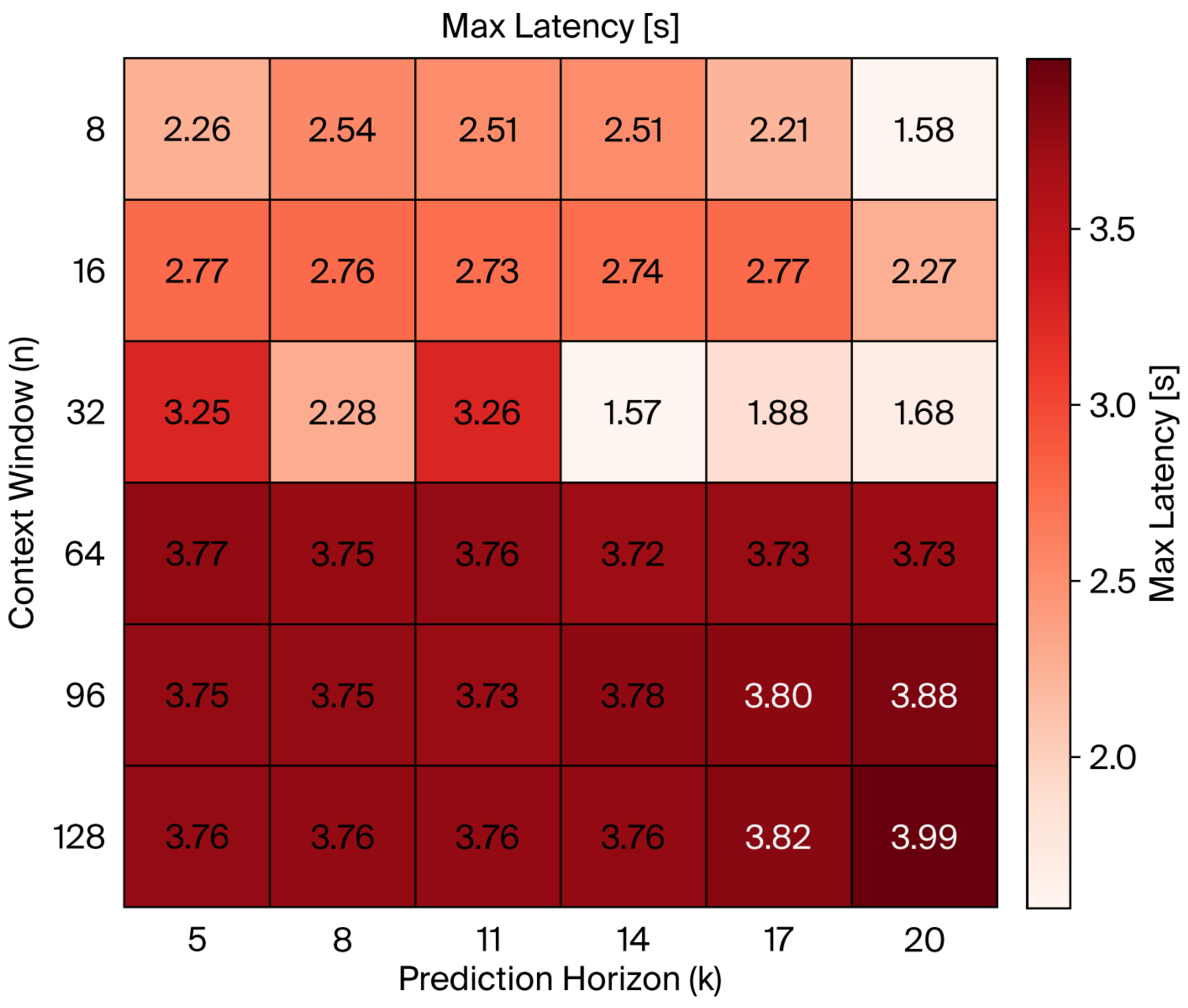
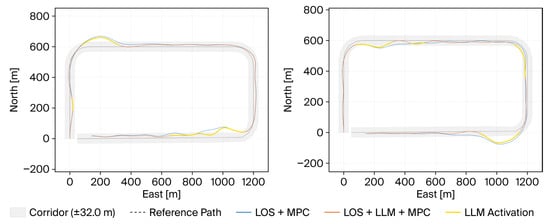
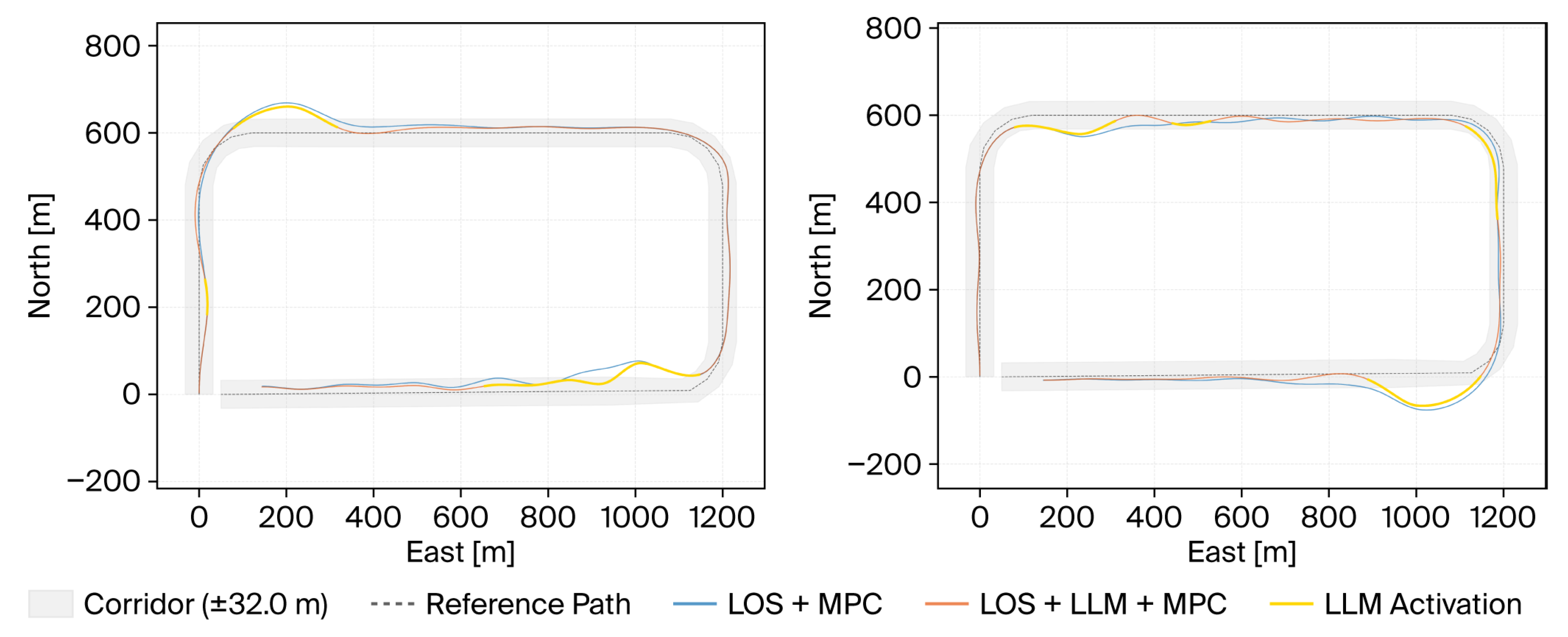
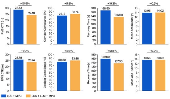
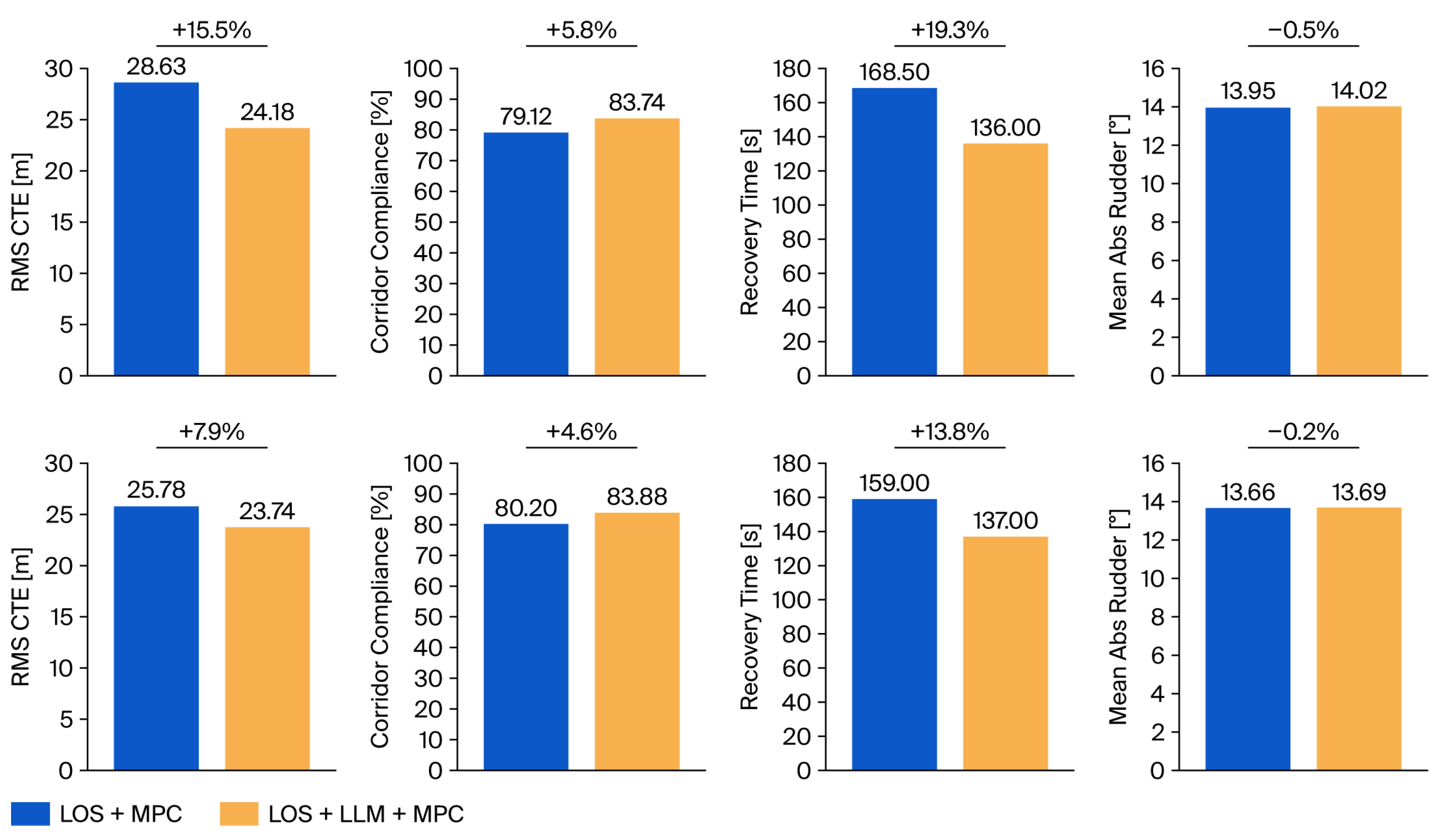
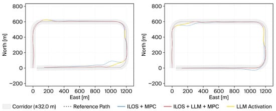
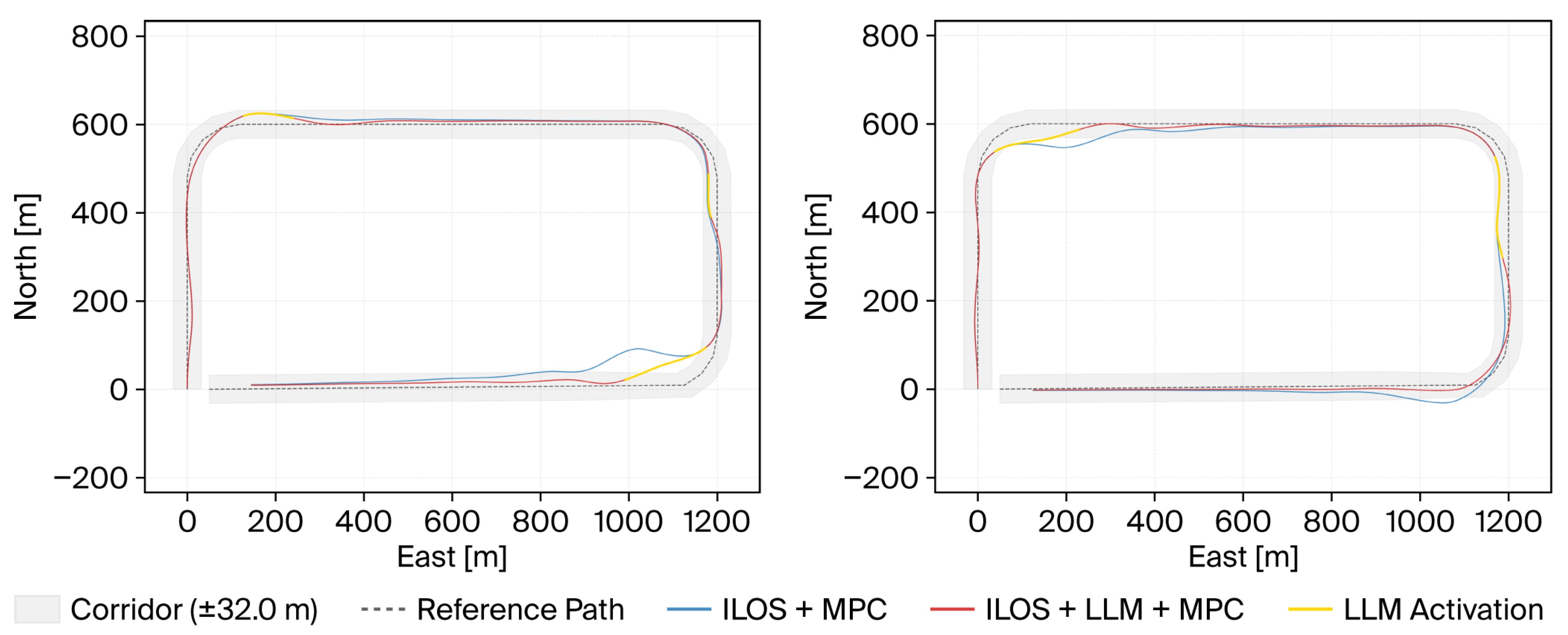
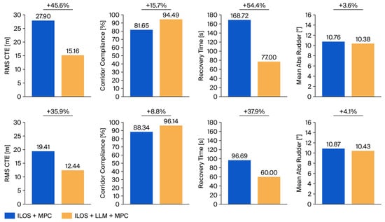
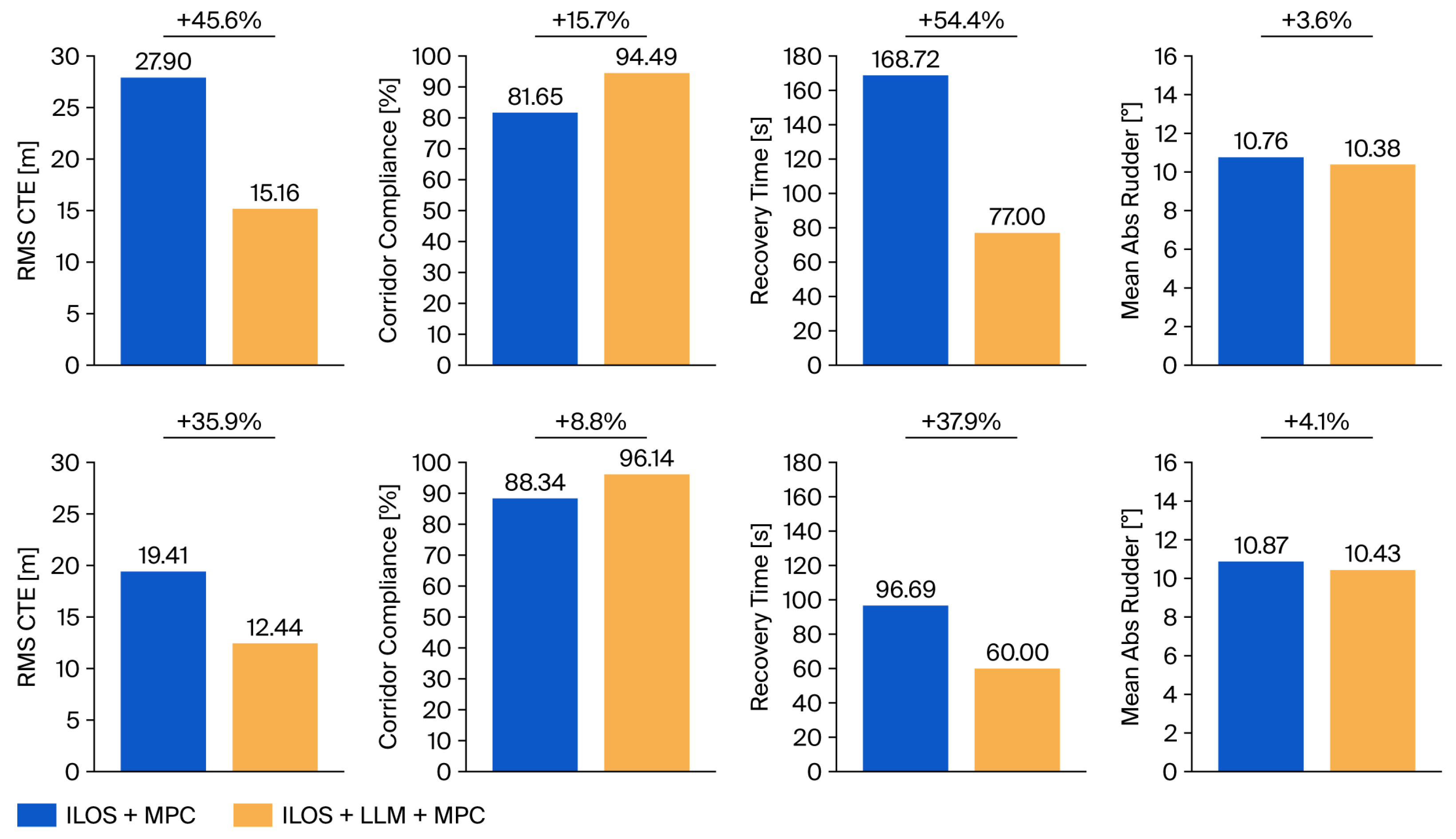
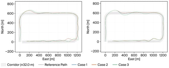
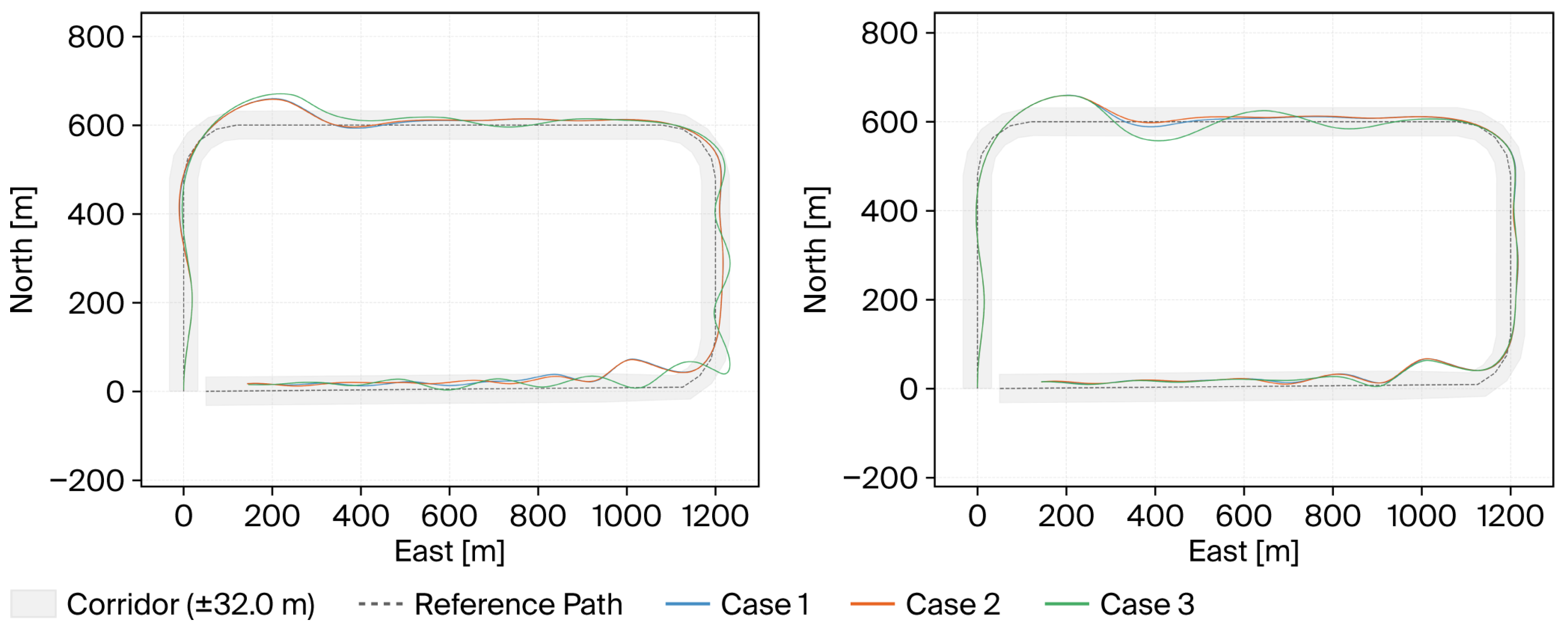
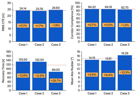
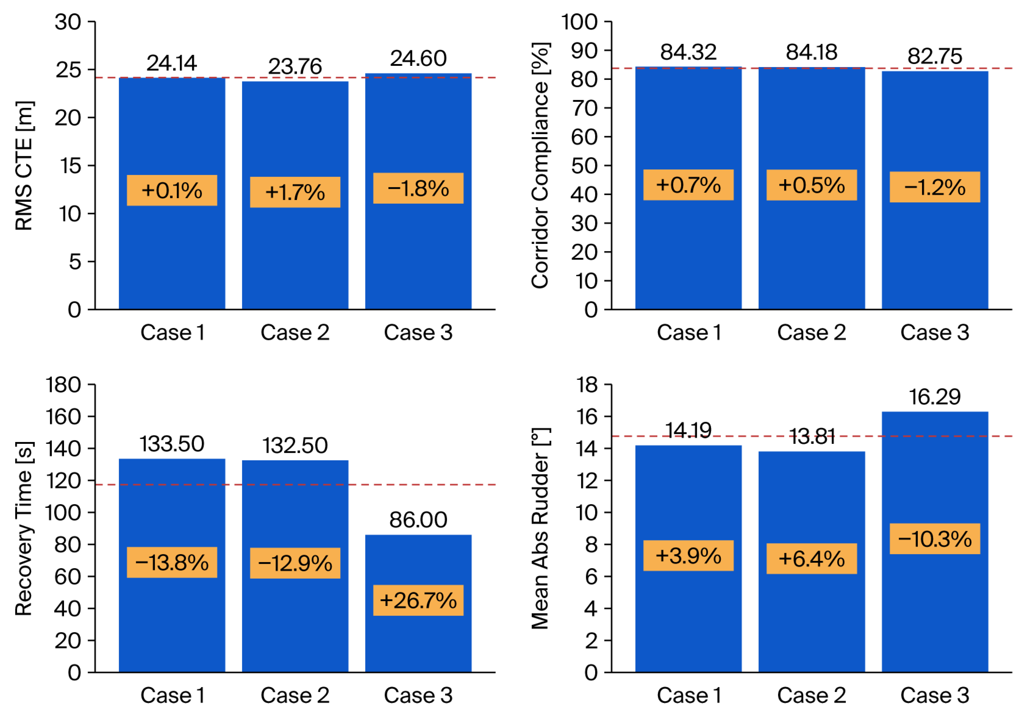
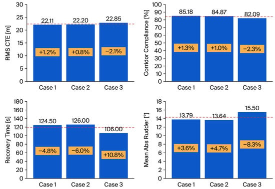
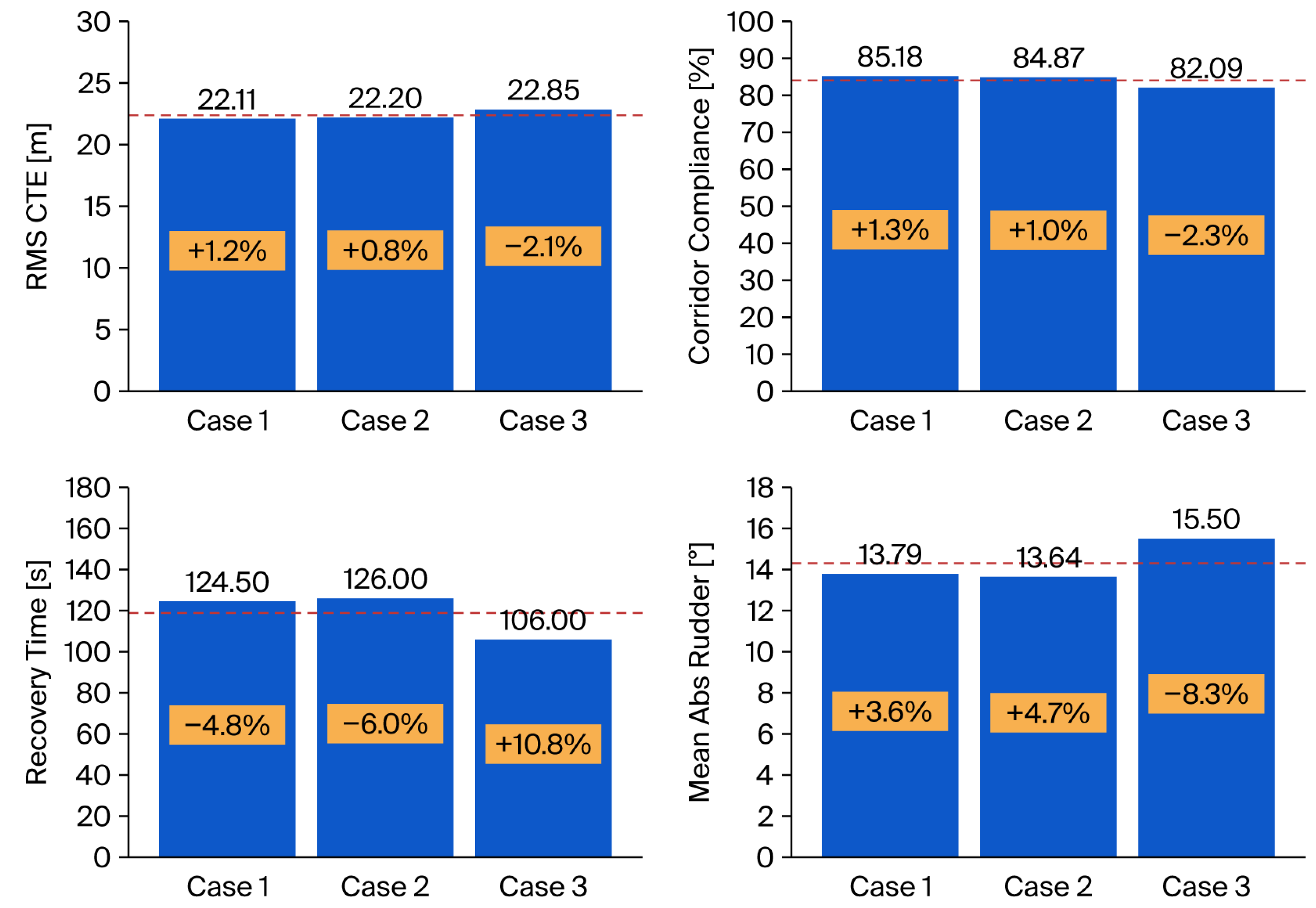

Disclaimer/Publisher’s Note: The statements, opinions and data contained in all publications are solely those of the individual author(s) and contributor(s) and not of MDPI and/or the editor(s). MDPI and/or the editor(s) disclaim responsibility for any injury to people or property resulting from any ideas, methods, instructions or products referred to in the content. |
© 2026 by the authors. Licensee MDPI, Basel, Switzerland. This article is an open access article distributed under the terms and conditions of the Creative Commons Attribution (CC BY) license.