


Abstract
Wind-assisted ship propulsion (WASP) has gained considerable interest as a means of reducing fuel consumption and Greenhouse Gas (GHG) emissions, with further benefits when combined with weather-optimized routing. This study employs and extends a National Technical University of Athens (NTUA) weather-routing optimization tool to more realistically assess WASP performance through integrated modeling. The original tool minimized fuel consumption using forecasted weather data and a physics-based performance model. A previous extension to account for the WASP effect introduced a 1-Degree Of Freedom (DOF) model that accounted only for longitudinal hydrodynamic and aerodynamic forces, estimating the reduced main-engine power required to maintain speed in given conditions. The current study incorporates a 3-DOF model that includes side forces and yaw moments, capturing resulting drift and rudder deflection effects. A Kamsarmax bulk carrier equipped with suction sails served as the case study. Initial simulations across various operating and weather conditions compared the two models. The 1-DOF model predicted fuel-saving potential up to 26% for the tested apparent wind speed and the range of possible headings, whereas the 3-DOF model indicated that transverse effects reduce WASP benefits by 2–7%. Differences in Main Engine (ME) power estimates between the two models reached up to 7% Maximum Continuous Rating (MCR) depending on the speed of wind. The study then applied both models within a weather-routing optimization framework to assess whether the optimal routes produced by each model differ and to quantify performance losses. It was found that the revised optimal route derived from the 3-DOF model improved total Fuel Oil Consumption (FOC) savings by 1.25% compared with the route optimized using the 1-DOF model when both were evaluated with the 3-DOF model.
1. Introduction
In recent decades, the International Maritime Organization (IMO) has implemented increasingly stringent regulations aiming to reduce the environmental impact and minimize ship emissions [1]. In response to the rising environmental concerns, the maritime industry has adopted more efficient and sustainable design and operational measures. Since fuel cost is considered the largest component of a vessel’s operating expenses, reducing the fuel oil consumption offers a dual benefit: regulatory compliance and significant cost savings.
Among the various design and operational measures proposed to reduce fuel consumption, wind-assisted ship propulsion (WASP) has gained substantial attention in recent years [2]. WASP includes a range of technologies that exploit wind energy to supplement a ship’s conventional propulsion system, thereby reducing engine load and lowering greenhouse gas emissions. Although the concept of wind-powered assistance is not new, modern advances in materials, automation, and aerodynamic design have enabled the practical deployment of WASP systems on ocean-going ships, while their modularity and flexibility make them particularly suitable for retrofitting existing vessels. The interest in WASP solutions is confirmed by the growth of the market in the last few years, with 28 installations done in the period 2010–2023, 26 installations in 2024 alone, and 22 new installations in 2025 (https://www.wind-ship.org/vessel-list/, accessed on 20 December 2025). Further growth of the market is expected in the near future, as foreseen by 2030 [3].
Common WASP technologies include Flettner rotors, wing sails, kites, and suction sails, where a detailed presentation of their operating principle provided in [2]. Each employ distinct aerodynamic principles to convert wind energy into useful thrust, and several vessels equipped with such systems have already demonstrated notable fuel savings, confirming that wind energy can meaningfully contribute to maritime decarbonization when integrated with traditional propulsion systems (e.g., [2,3]). Moreover, their performance benefits are especially pronounced on routes with favorable wind conditions. Notably, when combined with weather-routing optimization, the benefits of wind-assisted propulsion can be further increased and thus the use of weather routing together with WASP technologies is an effective way to increase energy efficiency and reduce greenhouse gas emissions.
However, predicting and evaluating the performance of wind-assisted ships in a realistic way is still challenging. Verifying the actual fuel-saving potential of these systems is important for both shipowners and technology developers. Recently, ITTC has started working toward standardizing methods for performance verification and monitoring of wind-assisted ships, covering both short-term and long-term evaluations [4,5]. Within this context, the usage of accurate performance models becomes essential, while it is also obvious that these models can also influence the identification of the weather optimal routes.
One key decision when building a performance model to estimate fuel savings is whether to use single-degree-of-freedom (1-DOF) or multi-degree-of-freedom (multi-DOF) approaches. In a 1-DOF model, only the longitudinal aerodynamic and hydrodynamic force components are considered. However, wind-assisted ships will usually operate in weather conditions that favor WASP efficiency but also could generate significant side forces and yaw moments. These asymmetric loads disturb the steady course of the vessel and create additional drag, which can reduce the expected fuel savings.
In Themelis [6], we extended a weather-routing tool developed at NTUA to include wind-assisted propulsion, allowing both measures to be considered together when evaluating the fuel-reduction potential. Although that study used a 1-DOF ship performance model, the optimal route obtained differed from the route identified without WASP integration.
The aim of the current study is to expand the ship performance model to a multi-DOF formulation and systematically examine the associated detrimental effects, quantifying the differences between the two model types. This comparison is intended to highlight the importance of using more advanced, or at least physically representative models in studies involving wind-assisted propulsion and weather routing. As a first step, the analysis will be carried out for a range of weather conditions, represented by apparent wind speed and direction, to compare the two models. A typical route will then be examined and optimized using the two ship model approaches, so as to investigate their impact on the resulting optimal path. In both cases, the assessment focuses on the performance losses due to the side-force effects.
In Section 2, a brief overview of related work is presented, while Section 3 presents the extended ship performance model along with key elements of the weather-routing tool. In Section 4 we apply the same case study as in Themelis [6]—using the same vessel, WASP configuration, and sailing route (Section 5)—to evaluate the differences arising from the two performance models, both in terms of overall fuel savings and the resulting optimal routes. Moreover, in Section 6, we discuss the main limitations of the study as well as future research directions. Finally, the main conclusions of the study are summarized.
As the performance of WASP continues to draw attention, this study introduces a 3-DOF physics-based model to provide a more realistic assessment, extending beyond our previous 1-DOF approach that neglects side forces and yaw moments. While the model involves certain simplifying assumptions, it is suitable for the scope of this work and for integration into weather routing optimization frameworks, as it directly solves algebraic equilibrium equations for drift and rudder angles, avoiding computationally intensive iterative time-domain calculations. Our work explores the impact of aerodynamic and hydrodynamic interactions on route selection, providing new insights into how these effects influence optimal routing and overall WASP performance. Controlled comparisons under identical operating conditions further quantify the consequences of neglecting these interactions.
2. Literature Review
This review focuses on the development of ship-performance models and their integration with route optimization tools. Early contributions, such as Bentin [7], established the foundation for integrating WASP performance within voyage planning by developing a routing optimization tool that couples theoretical modelling with onboard measurements. This study demonstrated the feasibility of incorporating WASP-specific aerodynamic forces into voyage simulations. Viola [8] introduced a coupled time-domain model to evaluate wing-sail performance on tankers. Their results demonstrated that, even under favorable wind conditions, realistic fuel-saving potential is often modest unless devices are exceptionally efficient. For example, in favorable wind conditions, optimized wing sails reduced propeller thrust by only about 10%. Thus, oversimplified or decoupled models often exaggerate WASP performance due to omission of course-keeping, as well as aerodynamic and hydrodynamic force-interaction effects. Ammar and Seddiek [9] investigated the environmental and economic performance of Flettner rotors installed on a bulk carrier. Simplified force balance assumptions are used, neglecting any drift and rudder effects. The study evaluates wind-assisted propulsion across three different routes to estimate fuel savings, emissions reduction and the corresponding payback period of the investment. In addition, the generated thrust and the net output are evaluated over a wide range of true wind speeds and directions, highlighting the maximum benefits at near beam conditions. The results show notable savings (up to 16%) but also strong dependence on route-specific wind statistics. Higher-order modelling is also lacking in a similar approach proposed by Vigna and Figari [10]. The methodology relies on integrating Flettner rotors into a conventional diesel propulsion parametric model, focusing on engine and Controllable Pitch Propeller (CPP) working points. The parametric modelling enables systematic explorations of the geometry of the Flettner rotors, propeller pitch and engine size, evaluating different operating points under varying wind conditions.
On the other hand, Van der Kolk et al. [11] demonstrate how hydrodynamic forces and moments act on ships operating at leeway angles. Through extensive towing tank experiments and numerical simulations, it is highlighted that induced leeway angles, side forces, yaw moments and respective resistance components may mitigate the thrust generated by a wind propulsor. For a realistic performance assessment, it is strongly recommended to account for lateral force balance and yaw moment equilibrium, rather than relying solely on longitudinal force balance. Moreover, Tillig and Ringsberg [12] showed that incorporating surge, sway, yaw, and heel dynamics through a four-degree-of-freedom (4-DOF) model leads to markedly different predictions of fuel consumption compared to simplified 1-DOF resistance-only models. Over a full voyage, the accumulated effect on fuel consumption was substantial: the 1-DOF prediction showed about 20% fuel savings due to the rotors, whereas the more realistic 4-DOF simulation showed only about 13% savings, a difference of about 7 percentage points that is attributed to the critical role of yaw moments and rudder-induced resistance when evaluating WASP performance. Continuing their work, Tillig and Ringsberg [13] present a novel approach for wind assisted ships, that accounts for aero- and hydrodynamic interaction effects—specifically between the sails and the superstructure. A 4-degree-of-freedom performance model (ShipCLEAN) is utilized to capture surge, sway, roll and yaw, which also includes a controlling method for optimizing rpm of Flettner rotors to maximize their impact on fuel oil consumption. The model is validated both with model-scale and full-scale data, and respective case studies for a tanker and a RoRo vessel are presented. The vessels are tested under different configurations with multiple Flettner rotors. The results show that neglecting lateral forces and yaw moments can lead to significant mispredictions of fuel savings of such systems.
Ma et al. [14] integrated wind-resource mapping with a dynamic WASP performance model (3-DOF) to predict annual energy savings along typical tanker routes, achieving an estimated 5.5% reduction for a Very Large Crude Carrier (VLCC) equipped with wing sails, highlighting the importance of representing sail forces in balance with rudder loads. Ghorbani et al. [15] presented a high-fidelity simulation tool that incorporates hull dynamics, rudder forces, controllable-pitch propellers, main-engine characteristics, and suction-sail aerodynamics. The model was validated using sea-trial and voyage operational data, and the analysis showed that maintaining constant vessel speed with variable wind assistance resulted in higher fuel savings than simply increasing ship speed during favorable winds.
From another perspective, earlier studies highlighted the importance of accounting for hydrodynamic and aerodynamic side forces as well as yaw moments to avoid overestimating the potential benefits of wind-assisted propulsion. In particular, when a vessel experiences asymmetric loading, the forces required to maintain a steady course cause it to sail with a drift angle. This drift angle, combined with the necessary rudder deflection, generates additional hydrodynamic forces that must be considered in performance assessments.
Skogman [16] carried out one of the earliest systematic analyses of the above-mentioned lateral balance problem in wind-assisted ships, by defining an equilibrium between aerodynamic and hydrodynamic moments about the ship’s center of gravity. While his approach was based on the dynamic maneuvering model of Inoue [17], which represents surge, sway, and yaw motions through coupled nonlinear equations, he neglected the time-dependent terms, and he assumed steady-state conditions. This practical approach in terms of computational effort showed that even small leeway angles can significantly increase total resistance.
Elger et al. [18] advanced Skogman’s framework by evaluating several methods for predicting drift and rudder forces and validating them with model tests. Their work highlighted the key role of the horizontal alignment between the aerodynamic center of pressure and the hull’s center of lateral resistance, the offset of which generates a yawing moment requiring rudder correction. They reformulated and validated Skogman’s static approach for modern cargo and wind-assisted vessels, showing good agreement with experiments for moderate drift angles, while noting that larger Aerodynamic Center of Pressure–Center of Lateral Resistance (ACP–CLR) separations lead to underestimation due to the model’s linearized assumptions.
Existing research on the subject has approached WASP systems from other perspectives as well. For instance, Marie and Courteille [19] introduce a fuzzy-logic-based fuel consumption model, which enables flexible and vessel-independent modeling of fuel consumption, especially for vessels equipped with WASP systems. Instead, it is based on environmental conditions and direct on-board measurements, creating a fuzzy-data-driven system that can be adapted to different vessels without extensive re-calibration. The applicability of fuzzy logic modeling becomes particularly evident in the context of WASP systems, where wind contribution is inherently variable, stochastic and route dependent. Additionally, Reche-Vilanova et al. [20] present a design optimization tool for Wind Propulsion Systems (WPS) that enables cost–benefit analysis. Their study goes beyond conventional WPS performance evaluation by combining different route simulations, feasibility constraints and fuel prices to identify the optimal WPS configurations for a specific vessel. The presented case study also highlighted that the payback period of the system can be 150% higher when the installed configuration is optimized.
3. The Extended Weather Routing Tool Incorporating WASP
3.1. A Brief Review of the Ship Model
The weather-routing tool employed in the study was developed at NTUA and implemented in the MATLAB environment (MATLAB R2024b), taking advantage of a wide range of built-in functions and specialized toolboxes, such as the Mapping and Regression Toolboxes. It can assist the ship master in the decision-making process, with the primary objective of reducing Fuel Oil Consumption (FOC). In addition, the tool features a high degree of modularity, enabling users to integrate alternative methods or incorporate different datasets as needed. Further details regarding the tool’s architecture and the optimization procedure can be found in [21,22].
The Ship Model is the core component of the tool and serves as a key element of the computational framework, as it enables the estimation of the Main Engine’s Fuel Oil Consumption (ME FOC). The model incorporates data related to the vessel’s total resistance, as well as technical characteristics of the main engine and propeller. The various resistance components are computed for specific operational conditions, including vessel speed, mean draft, and encountered weather conditions. In addition, the model accounts for the main engine’s Specific Fuel Oil Consumption (SFOC) map across different load and RPM values.
The initial version of the Ship Model focuses on longitudinal equilibrium using the following equation:
where the calm water resistance component () can be determined from experimental resistance curves from towing-tank tests or from computational fluid dynamics (CFD) analysis, whereas the mean added wave resistance in an irregular sea () is estimated using empirical or semi-empirical methods for the added wave resistance in regular waves (such as [23,24]) combined with spectral analysis. In the current study, the empirical formula of [24] is utilized to calculate the added wave resistance in regular waves and the JONSWAP wave spectrum is employed. In addition, the calculation of wind resistance () is based on the calculation of wind coefficients, for which various methods could be employed, including semi-empirical formulas, wind tunnel experimental data, and CFD simulations. For this study, the wind resistance was evaluated using Blendermann’s method [25], which employs a semi-empirical loading function derived from wind tunnel tests. Lastly, is the thrust generated by the propeller to balance the total resistance and enable the vessel to operate at a specified speed.
The required thrust from the propeller is combined with its open-water characteristic curves to estimate its RPM; consequently, the required power and revolutions by the main engine (ME) can be calculated. For any pair of ME brake power revolutions (PB, n), the SFOC can be also calculated. Each candidate route is defined by a series of waypoints that shape the overall trajectory, making the vessel alter its course at each of these points. In addition, the route is divided into discrete points (xi), where the SFOC is computed at each one [22]. Together with the ME power and the passage time between the points, the total ME FOC of the voyage can be obtained by summing up the ME FOCi calculated between each consecutive pair of these points (FOCi).
The minimization of the total ΜΕ FOC is then used as the objective function and an optimization process is applied to determine the optimal trajectory among a series of candidates generated according to a genetic algorithm that is utilized from MATLAB’s Optimization Toolbox [26]. To solve this optimization problem, the algorithm adjusts the waypoints’ geographical coordinates while the population progressively evolves towards the optimal solution over successive generations:
3.2. Ship Model Incorporating WASP (1-DOF)
The ship model was expanded in [6] to include the effect of a WASP on the ME power needed to sustain a specific ship speed and consequently on the required fuel consumption, by incorporating into Equation (1) the thrust force produced by the WASP (:
This approach (1-DOF) simplifies the problem by neglecting all transverse forces and yaw moments, retaining only the longitudinal contribution of the WASP system. If the system requires auxiliary power for its operation, this power is assumed to be provided by the vessel’s diesel generators and is added to the ME FOC to form the total FOC. In addition, interactions between the sails and/or between the sails and the hull are neglected in the analysis, while the system is also assumed not to affect the added wind resistance in any way.
However, such an assessment would over-predict the gains of the WASP as the system generates not only forward thrust but also transverse forces. To maintain a steady course under this asymmetric loading, which, in the case of WASP operation, will be more pronounced as the ship seeks to operate in near-beam wind conditions where WASP efficiency is higher, the ship balances these later forces by sailing with a small leeway (drift) angle and rudder deflection. This creates extra resistance because the hull moves at an angle and produces side force such as a low-aspect-ratio wing, while the rudder also generates lift with its own drag penalty. Therefore, a proper assessment requires a consideration of the vessel’s balance both in lateral forces and yaw moments, which influences total resistance and maneuverability. This extension of the analysis is presented in the following sub-section.
3.3. Ship Model Incorporating WASP (3-DOF)
As noted previously, aerodynamic transverse forces and yaw moments are present due to lateral aerodynamic loads and become greater with the installation of WASP systems on board. In practice, excessive transverse forces, yaw moments and/or improper longitudinal WASP configurations can result in significant rudder deflection, degrading steering capability. To address these conditions and for a more realistic approach, the ship model is expanded to account for transverse forces and yaw moments using 3-equations modelling (3-DOF) instead of 1-equation (1-DOF) modelling. The consideration of the generated forces and moments from both the wind and the WASP results in drift creation generating hydrodynamic forces and yaw moments, as well as forces acting on the rudder, which counterbalance the vessels forward motion. Therefore, the induced drift angle and rudder deflections produce additional resistance forces in the longitudinal direction.
The equilibrium can hence be described with the following equations:
where and denote a yaw moment and a lateral force, respectively, while the subscript indicates its source. denotes the hull hydrodynamic component caused by drift and the rudder-induced component.
Equation (3) is reformed as follows:
Similarly, denotes a longitudinal force related to its subscript each time.
There are many methods in the literature for calculating drift (β) and rudder (δ) angles; however, the first method is derived from [16] and uses equations originally presented by [17]. Skogman’s equations are modified to provide the angles (drift and rudder) as output. Specifically, this method is derived from the dynamic maneuvering model proposed by Inoue [17] which represents ship motion in six degrees of freedom and incorporates nonlinear, time-dependent surge, sway, and yaw terms. While Inoue’s formulation is appropriate for predicting transient maneuvers and assessing course stability, it is computationally intensive and relies on the iterative integration of the motion equations.
Skogman simplified this framework by not considering the acceleration terms and assuming steady, straight-ahead motion at constant speed. The assumptions form a quasi-static model in which forces and moments are balanced around the center of gravity without any time dependence. As a result, the drift angle (β) and rudder angle (δ) can be obtained directly from algebraic relations, eliminating the iterative evaluation of hydrodynamic derivatives and motion responses required in Inoue’s original approach.
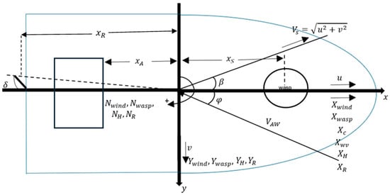
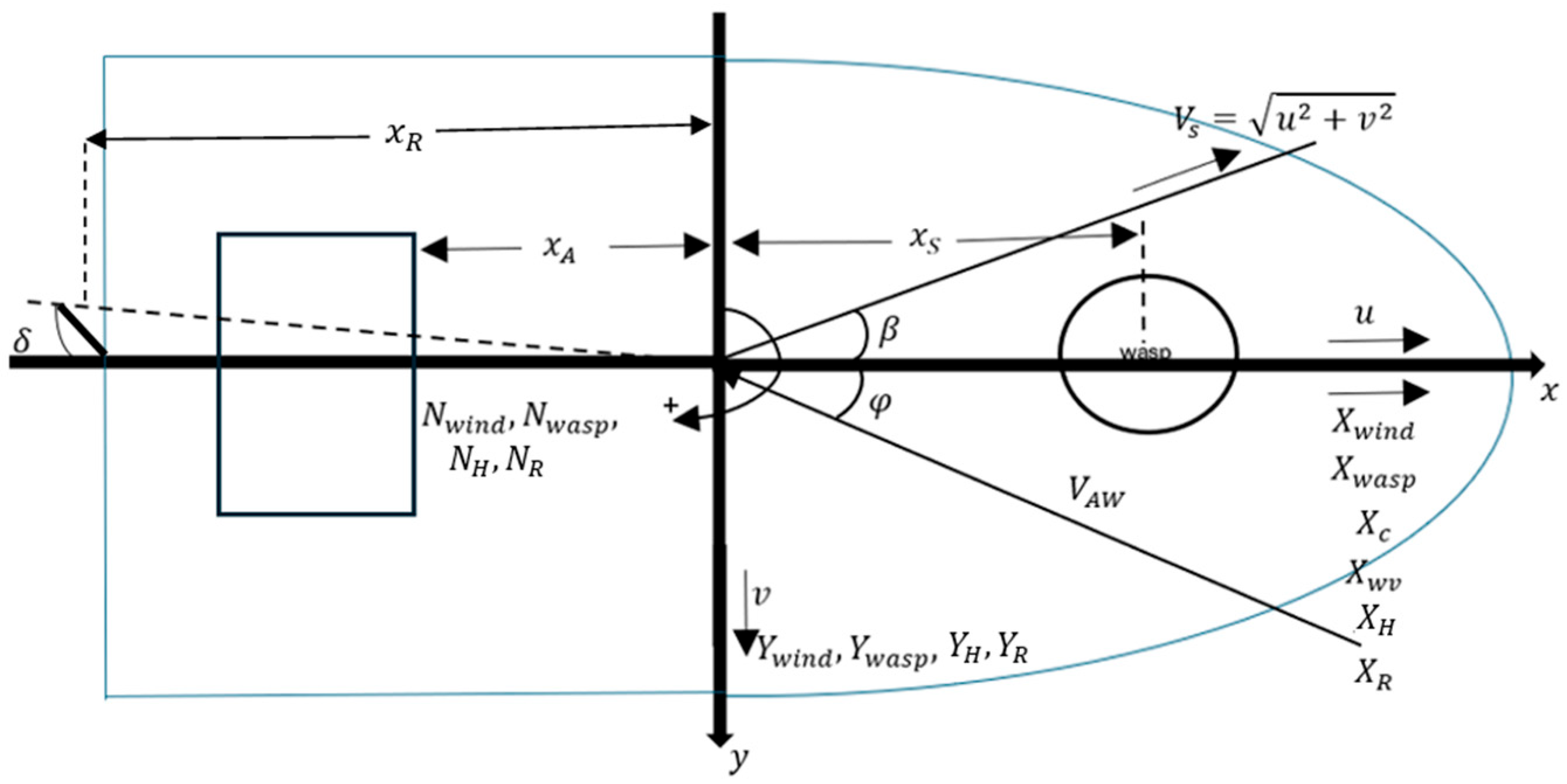
To simplify calculations, the center of gravity is placed at the midship section (Figure 1). In the coordinate system used, the x-axis points forward along the ship’s length, and the y-axis is positive towards the starboard side.
Figure 1.
Forces in the 3-DOF ship model including WASP.
The terms appearing in Equations (4) and (5) are estimated as follows. First, the yaw moment due to WASP, is derived as:
where is the transverse force created by the wind due to the WASP system and should be taken as negative when it comes from starboard, and denotes the longitudinal distance between the point of application of and the ship’s center of gravity (Figure 1). In addition, is transformed as follows to be in accordance with the coordinate system:
where is the air density, is the lateral windage area, is the apparent wind speed, is the non-dimensional aerodynamic yaw moment coefficient and is the overall length of the vessel.
The aerodynamic lateral force is also transformed as follows:
where is the non-dimensional aerodynamic lateral force coefficient. The hydrodynamic moment is:
The geometric effective aspect ratio of the rudder is:
The effective aspect ratio is:
where , , and are dimensions of spade rudder, as defined by the symbols in [18].
The hydrodynamic transverse force is determined as:
where the lateral force’s hydrodynamic derivatives are:
is the dimensionless sway velocity and is the underwater portion of the hull’s effective aspect ratio:
Assuming a rudder deflection , the lateral rudder force and rudder moment are:
A force factor is applied to represent the hydrodynamic force exerted on the ship’s hull due to rudder action, and specifically is defined as the ratio of the hull force generated by the rudder to the rudder force itself and is derived through regression analysis from model testing [18].
Moreover, , as the lever arm distance from the rudder’s pressure point to the midship and the normal rudder force assuming an initial arbitrary inflow angle (e.g., 5°), is:
The inflow speed to the rudder is reduced by the wake :
According to Skogman [16], from Equation (4), we solve the term and then use its solution in Equation (5). To simplify the terms, an additional parameter (see also [16,17]) is used:
where is the water density, is the draft, and is the waterline length.
The equation that is derived is a normal equation of the second degree, considering that is always negative and the dimensionless sway velocity is negative when the vessel moves forward for the chosen reference system:
The dimensionless drift speed is then derived as the negative root with the smaller absolute value:
Then the drift angle can be obtained as:
Also, the ship’s speed in x-direction is:
Knowing the dimensionless drift speed, from Equation (4), the equilibrium rudder angle can be derived as:
Then the inflow angle is calculated according to the next equation and the rudder force shall be calculated again until convergence is achieved:
The added resistance due to the rudder and the lateral rudder force is:
Moreover, the added resistance due to drift can be derived from the formula:
where the non-dimensional added resistance factor due to drift is:
which is a third-degree curve regression derived from model tests of different vessel types [18], where is in degrees.
4. Examined Ship and WASP Implementation
4.1. Vessel Specifications and WASP Configuration
The vessel considered in the current study is a Kamsarmax-type bulk carrier and its main characteristics are reported in Table 1.
Table 1.
Ship’s main characteristics.
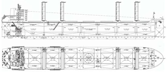
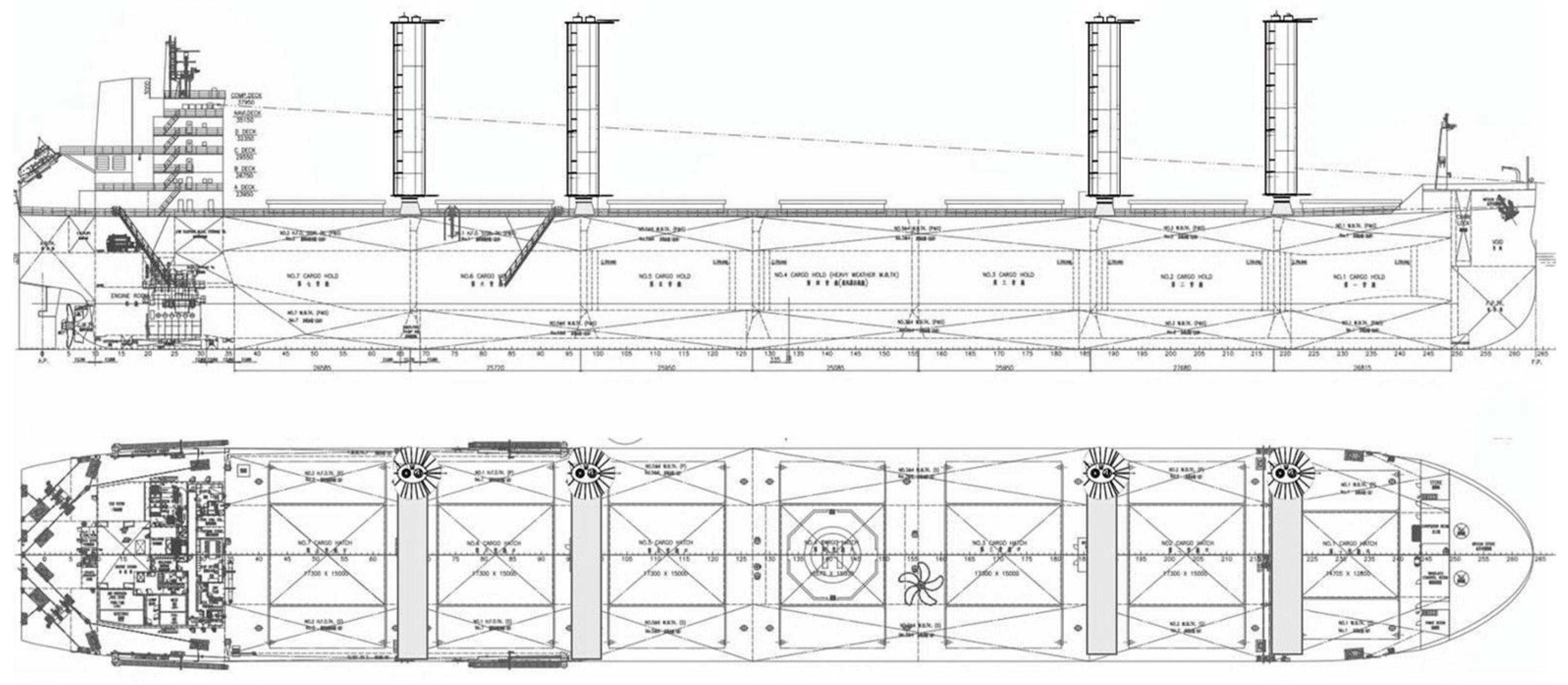
A suction-type sail WASP system is integrated into the existing weather routing tool, to evaluate its impact on the fuel oil consumption. The WASP setup includes four suction sails at the locations shown in Figure 2. Suction-type sails can enhance aerodynamic lift by pulling air into the sail structure, preventing air flow separation and allowing the system to generate extra thrust.
Figure 2.
Arrangement of the four suction-type sails.
Available data regarding WASP forces (driving and transverse forces), as well as the required power for the system to operate, are utilized to train regression models over a broad range of apparent wind speeds and directions, reducing the computational time of the required calculations (more details, regarding regression type, accuracy metrics, inputs etc., can be found in [6]).
4.2. Preliminary WASP Assessment
For the present study, the vessel is considered to travel at a speed of 11 knots with a loading condition at the scantling draft of T = 14.45 m. This particular speed corresponds to the average operational speed at which the vessel operated during a significant period of time at the same draft. The weather conditions are characterized by a significant wave height of 2 m and a peak wave period of 10 s, while the true wind speed is 7.5 m/s (Table 2). For this analysis, wind and waves originate from the same direction. The calculation of the added wave and wind resistance follows the description provided in the previous section.
Table 2.
Weather and loading conditions for the case study.
As discussed above, the operation of a WASP system introduces additional side forces and yaw moments that need to be taken into account. As noted in the previous section, the induced drift and rudder angles should be calculated to estimate ship’s performance and, additionally, the added resistance caused by the drift and the rudder, since these components contribute to the total resistance and consequently to the required power from the main engine. This study demonstrates how the 1-DOF and 3-DOF ship models provide different results regarding the WASP’s performance. Various cases of modelling have been analyzed regarding the use of the WASP system with the four suction-type sails, as discussed in the previous sections, which include or neglect the side forces and yaw moments.
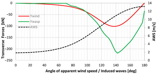
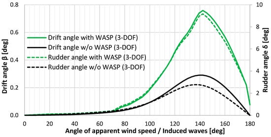
In Figure 3, the generated side forces, along with the prevailing apparent wind speeds (AWS), are presented, while the corresponding drift and rudder angles are compared for different angles of apparent wind, both with and without WASP, in Figure 4. Their peaks are found around 140 degrees of apparent wind, where the transverse forces are significantly high. Given the assumed wind conditions, around 140 degrees of apparent wind angle, the sails operate near their optimal aerodynamic state, where the generated lift is maximized but at the expense of pronounced side forces. Notably, it is assumed that head wind (true and apparent) corresponds to 180 degrees for all upcoming results.
Figure 3.
Transverse forces and AWS vs. apparent wind direction.
Figure 4.
Drift and rudder angles vs. apparent wind and wave direction.
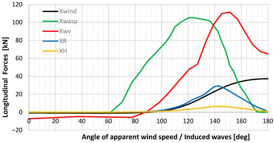
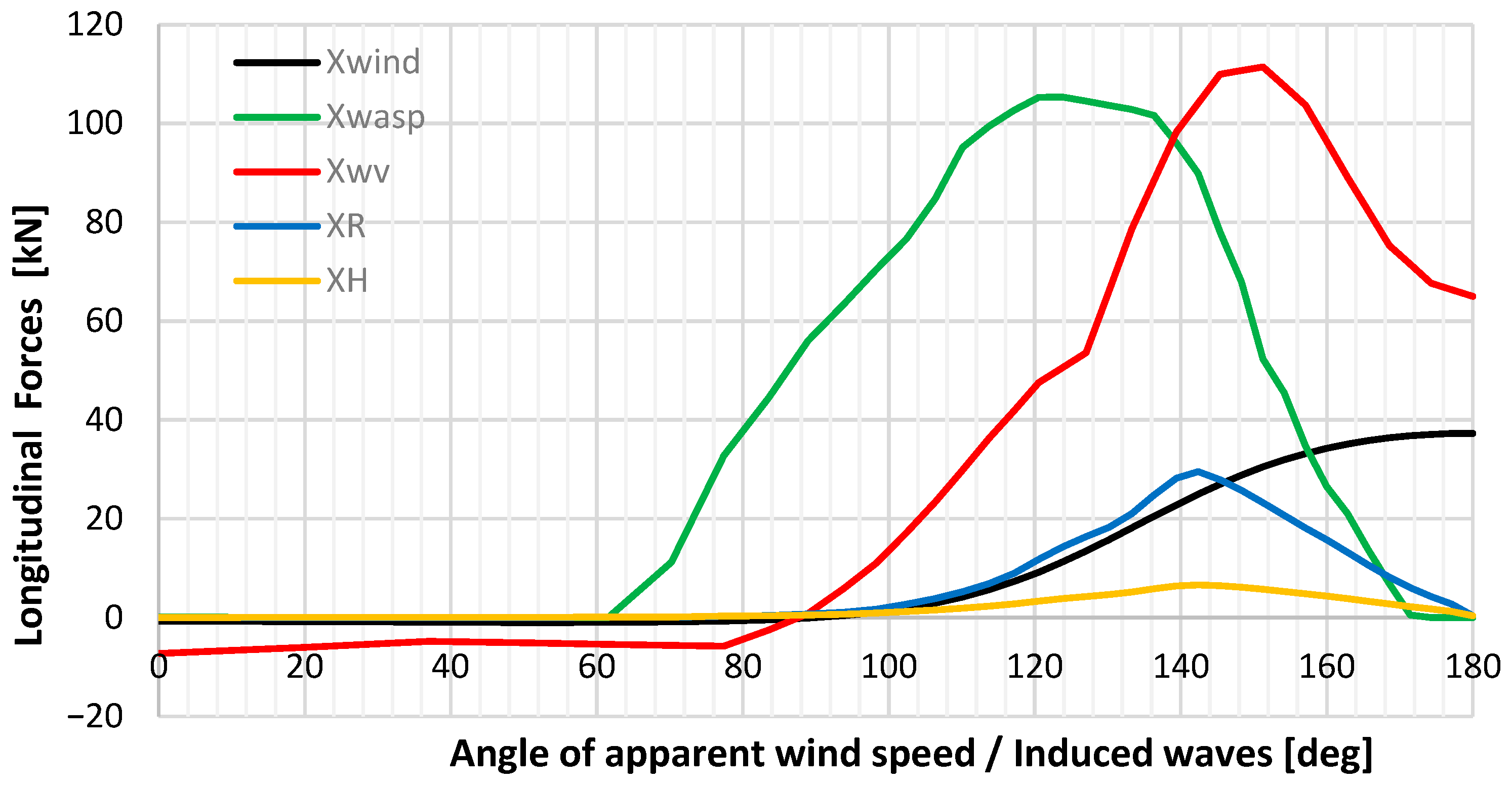
As expected, the longitudinal component of the rudder resistance is also high at the same wind angles. All the longitudinal forces are presented in Figure 5, and the calm water resistance remains constant at 406.93 [kN]; however, it is omitted from Figure 5, to maintain clarity in the graph. The added wave resistance increases significantly for relative wave (and wind for the presented example) headings between beam and bow. The same trend is observed for the wind resistance component; however, the magnitude of the increase is notably lower, as expected given the smaller influence of wind loads compared to induced wave forces for a large cargo vessel. Regarding the drift and rudder effects, their peaks are also formed around 140 degrees of apparent wind direction. Their magnitude also differs, indicating that the influence of the WASP system is primarily depicted through rudder deflection.
Figure 5.
Longitudinal forces vs. apparent wind direction.
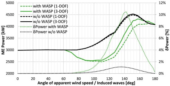
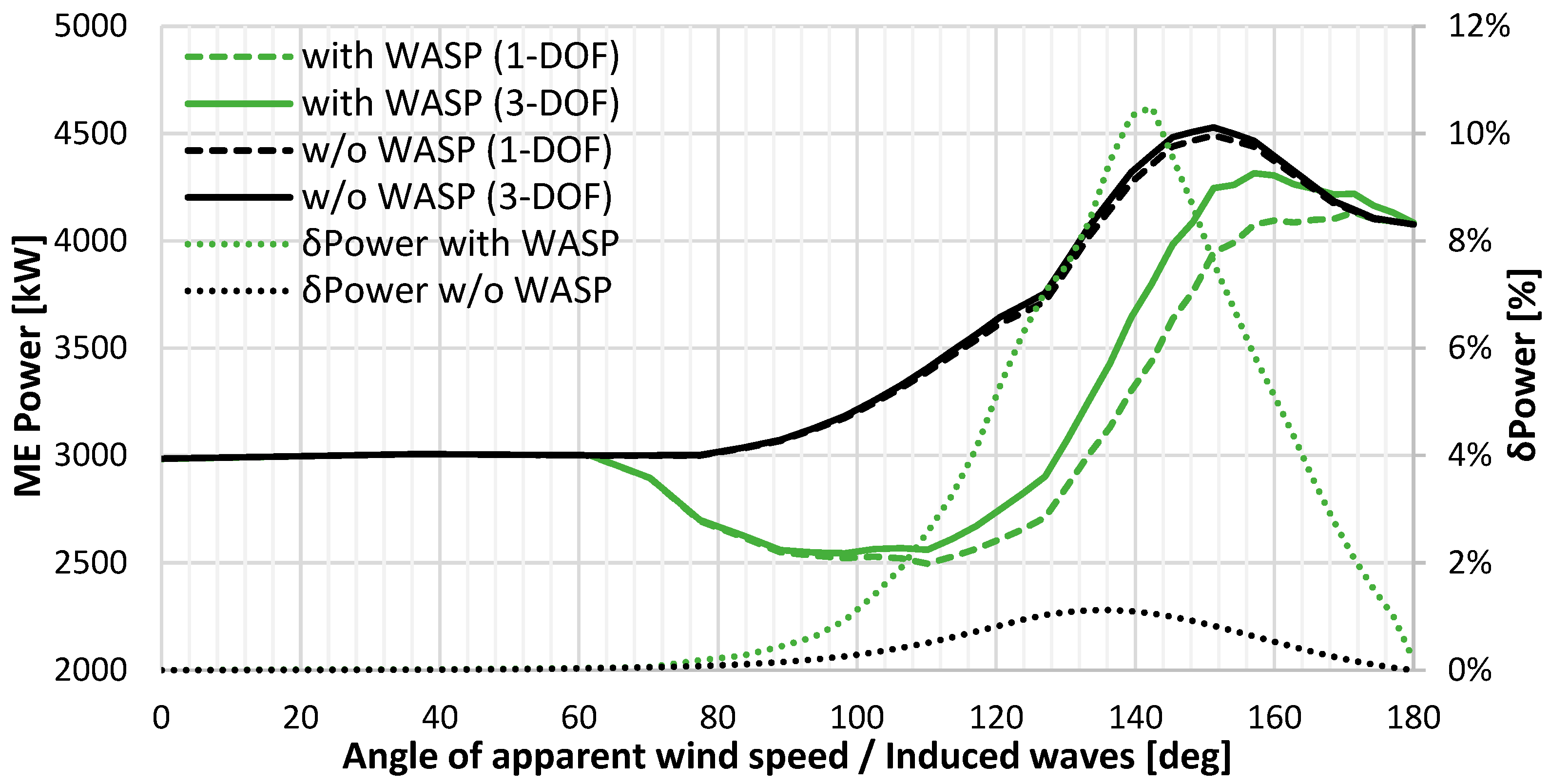
Figure 6 shows the main engine power, comparing cases where the WASP system is installed versus not installed, as well as scenarios with and without the consideration of side forces and yaw moments in both cases. It is notable that, when the WASP system is not installed, the two models (1- & 3-DOF) present insignificant differences and, specifically, less than 1.5%, in the demanded power from the main engine under all possible apparent wind directions. However, WASP integration yields notable diversity in the required ME power values up to 10% between the two ship model approaches. This peak occurs at around 140 degrees of apparent wind direction, corresponding approximately to 5.5% MCR. Such systems tend to be more effective (i.e., produce more thrust) at around 90 degrees of true wind, namely, around 100–150 degrees of apparent wind direction depending on the prevailing wind speed. For the given true wind speed (7.5 m/s), the maximum thrust occurs at around 140 degrees of apparent wind direction, where the 1-DOF model also maximizes its power. On the other hand, when considering the 3-DOF model, gains regarding thrust from the WASP remain at a maximum around 140 degrees (Figure 5); additionally, the generated side forces (Figure 3) and yaw moments are high. This effect leads to rudder deflection and/or drifting, resulting in increased drag and, consequently, increased required power.
Figure 6.
ME power for scenarios with/without WASP system and considering the 1-DOF and 3-DOF ship models along with percentage differences in ME power between 1- and 3-DOF modelling with and without the WASP system.
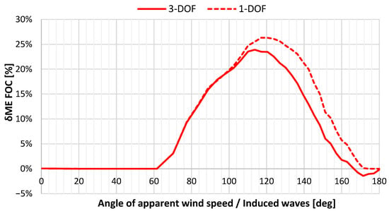
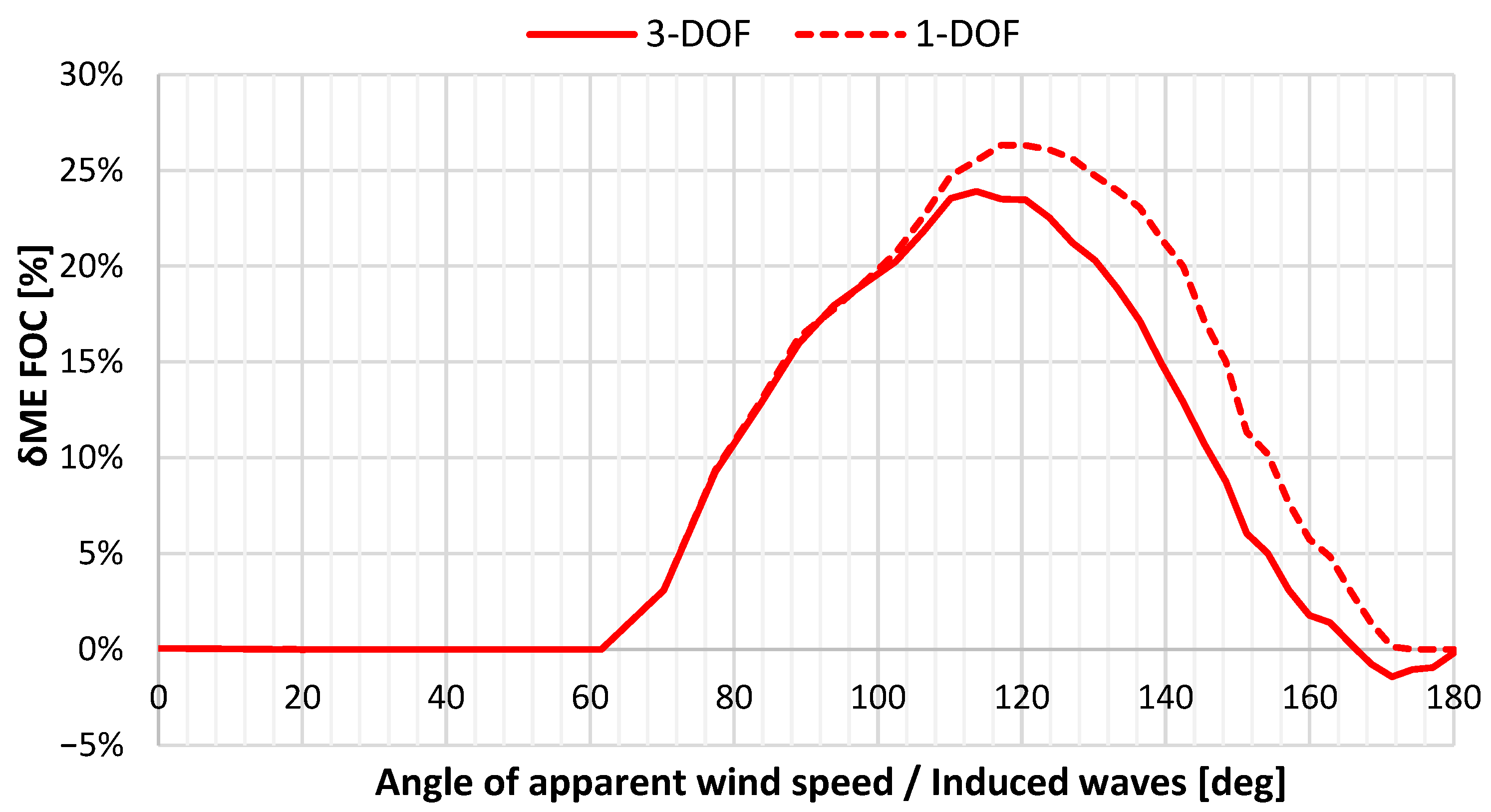
Moreover, Figure 7 shows the ME FOC savings with and without the WASP when using the 3-DOF and the 1-DOF Ship Model. When considering the 1-DOF modelling, ME FOC savings due to WASP reach 12.60% on average, while peaking up to 26% in favorable apparent wind directions, whereas these gains slightly drop when accounting for side forces and yaw moments bound up to an average of 10.14% and peaking up to 23.5%. Differences in ME FOC estimates between the two models range between 2 and 7%.
Figure 7.
ME FOC differences with and without the WASP system for the 3-DOF and 1-DOF ship models.
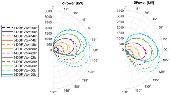
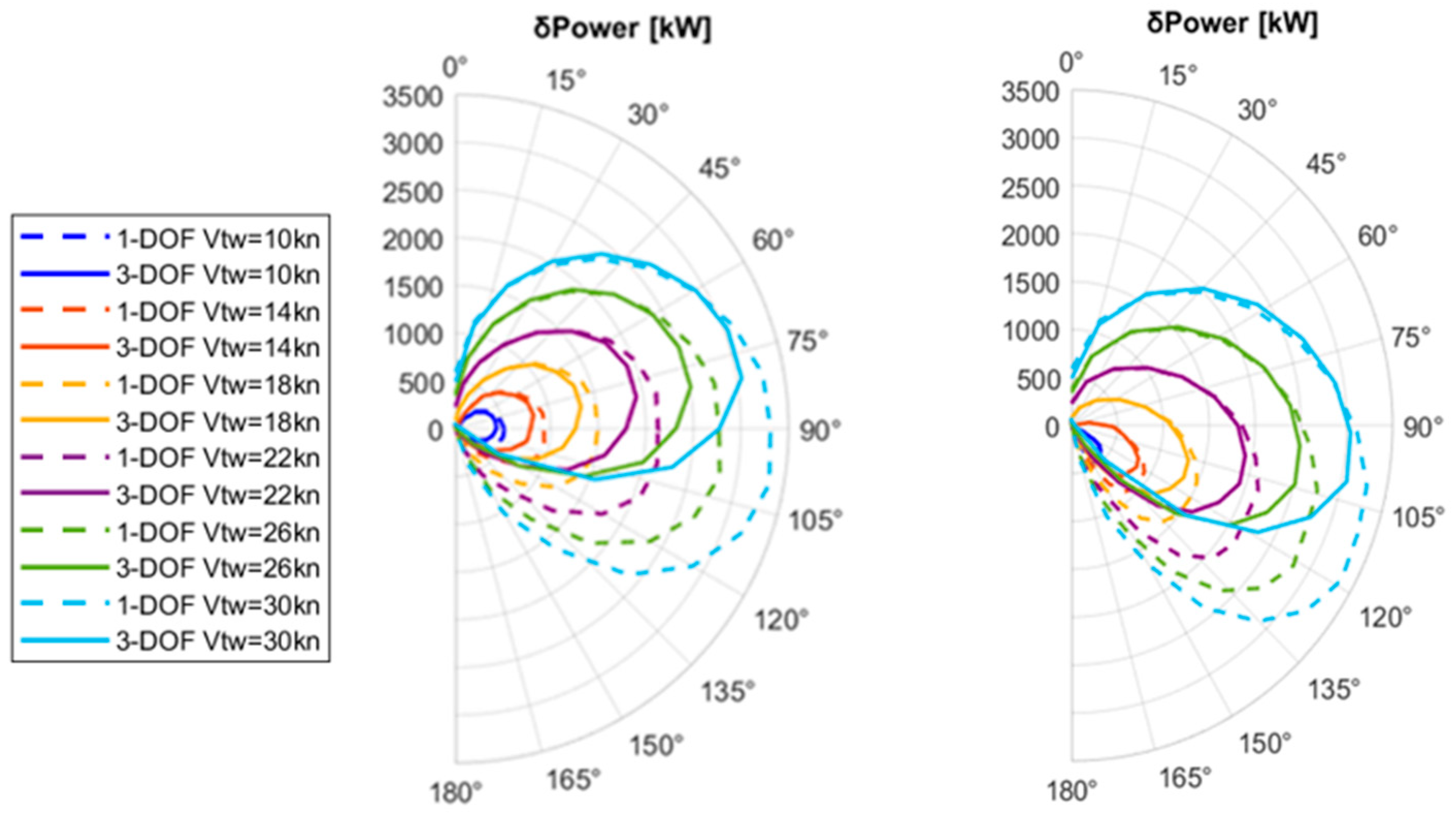
In addition, polar graphs have been created, considering the same ship speed and loading condition, illustrating the ΜΕ power savings achieved with the WASP system, both when considering the 1- and the 3-DOF (Figure 8) ship models. Calculations were performed considering various true wind directions within a 0–180-degree range for several values of true wind speeds, and the results are plotted against this range (Figure 8 left side) alongside the corresponding apparent wind direction (Figure 8, right side). The wave conditions and ship’s speed are kept the same as in Table 2. Pronounced differences between the two approaches are mainly observed from beam to bow apparent wind headings, where the WASP system is expected to be most effective.
Figure 8.
ME power savings for the 1- and 3-DOF ship model vs. the true wind direction (left) and apparent wind direction (right) for various true wind velocities .
Based on the results of Figure 8, the average ME power savings due to the WASP system are shown in Table 3, expressed as % MCR. The results show that increasing the wind speed leads to larger discrepancies between the two models—up to 7% MCR—highlighting the growing influence of transverse effects under higher wind conditions.
Table 3.
Average power savings in % MCR due to WASP for the 1- and 3-DOF ship model along with their percentage difference for the cases considered in Figure 8.
5. Case Study of a Specific Route
In this section, a simulation of a real past voyage of the examined bulk carrier is presented, along with results regarding optimal route planning under the same weather and loading conditions. Both the 1- and the 3-DOF ship models are applied, for the purposes of comparative analysis.
5.1. Examined Route and Set-Up of WASP Operation
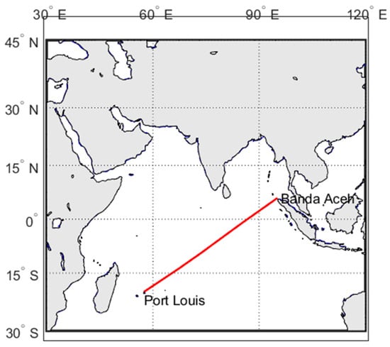
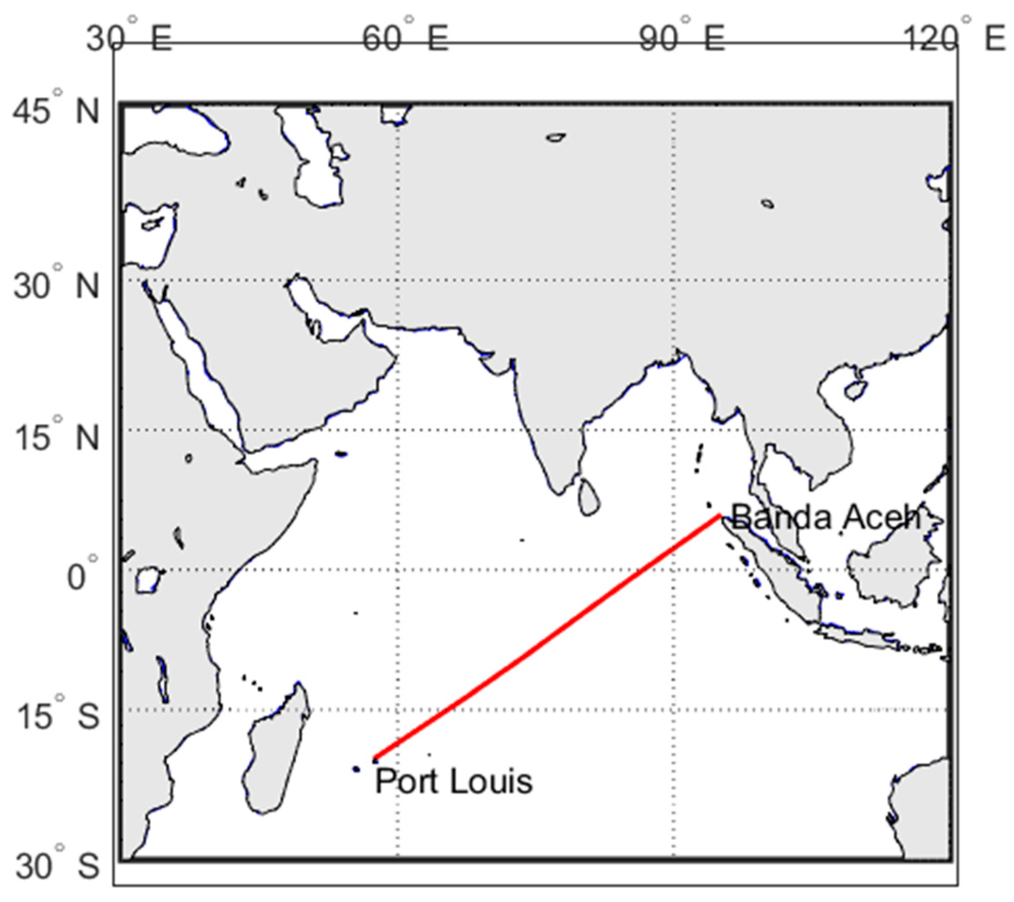
All of the following calculations and route optimizations concern a voyage started on 22 May 2022 at 13.30. The voyage is from Port Louis (Mauritius) to Singapore, but the conducted optimization focused on the voyage segment between Port Louis (Mauritius) and north of Banda Aceh (Indonesia). The remaining part of the voyage was not relevant to the route optimization process as it corresponds to operations in confined waters and was therefore excluded from the process (Figure 9). All marine environmental data were obtained from open-access datasets via Copernicus Marine Environment Monitoring Service (CMEMS). More specifically:
Figure 9.
Main segment of the real voyage selected for optimization, shown as a red line.
- Ocean currents with a spatial resolution of 0.083° × 0.083° and a 6 h temporal resolution (analysis and forecast product).
- Wave parameters with a spatial resolution of 0.083° × 0.083° and a 3 h temporal resolution (analysis and forecast product).
- Wind fields with a spatial resolution of 0.125° × 0.125° and a 1 h temporal resolution (blended observations product).
The nearest-neighbor approach was used to define values at locations outside the original data grid of each dataset. Moreover, for each dataset, the environmental conditions were assumed to be constant within the corresponding temporal resolution interval and replaced by the subsequent dataset snapshot.
For the optimization, a constant ship speed (about 11 kn) is assumed, which is the average speed calculated from the available noon reports for that specific part of the voyage. The optimization problem was solved by utilizing the built-in genetic algorithm (GA) of the MATLAB Optimization Toolbox [26]. We selected 100 generations and a population of 100 individuals, while a sensitivity analysis was conducted for these two main parameters, ensuring that these values led to convergence under a reasonable computational cost. The GA’s operators (selection, mutation, crossover, etc.) were assigned as the default MATLAB settings.
The necessary weather data were obtained from the Copernicus database, while the objective function of the optimization is the minimization of the total fuel oil consumption, considering the ME FOC and the consumption of the diesel generators, which operate along the transit. Additionally, a constraint regarding the maximum allowable rudder angle is also included by limiting the induced rudder angles to 35 degrees.
The same configuration of the WASP system examined previously is assumed. To calculate the total fuel consumption, the auxiliary power and fuel consumption have to be considered. The auxiliary power required for the operation of the WASP system is provided by the ship’s diesel generators. When the system does not provide a positive contribution to vessel’s propulsion, it is considered inactive. In addition, two diesel generators are available throughout the voyage. It is assumed that the first generator (DG1) operates at 400 kW, as the mean value from noon reports for the voyage, when the suction sails are not in use. The scenario defined sets that the DG1 can handle up to 600 kW when the suction sails are activated, with the remaining load distributed to DG2 if needed.
5.2. Voyage Simulation with WASP and Optimization
Results regarding the optimal routes derived by employing the 1-DOF version of the ship model (both with and without the WASP system installed) have already been presented in [6]. In the present analysis, the aim is to apply the 3-DOF version of the ship model to evaluate the optimal route previously identified using the 1-DOF model. This will allow for a comparison between the two models regarding the potential gains due to WASP, with particular attention to the adverse influence of side forces. Specifically, the optimal route found when the WASP is installed (1-DOF Ship Model) will be examined in the following cases:
- without (w/o) WASP and using the 1-DOF ship model,
- without (w/o) WASP and using the 3-DOF ship model,
- with WASP and using the 3-DOF ship model.
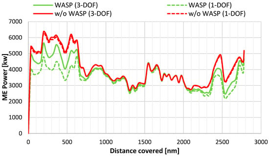
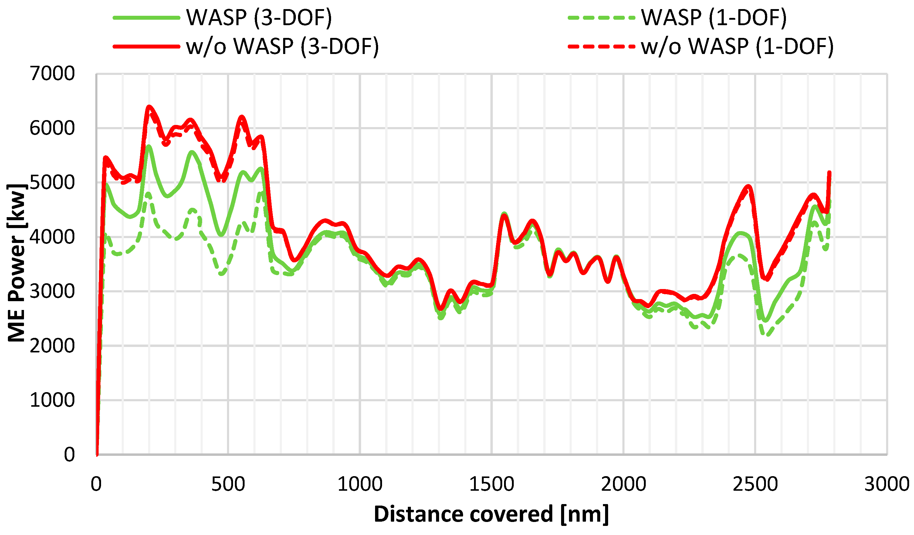
The ME power along the route for the above-mentioned scenarios is presented in Figure 10, whereas, in Figure 11, the apparent wind speed and its direction are shown. Regarding ME power, it is observed that, particularly during the first part of the voyage, the differences between the two approaches are more noticeable. This occurs because, in that sea area, the prevailing winds are stronger and more significant in the beam direction, which causes higher side forces and respective yaw moments.
Figure 10.
ME power with and w/o WASP for 1-DOF and 3-DOF for the optimal path.
Figure 11.
Prevailing wind conditions for the optimal path corresponding to 1-DOF ship model.
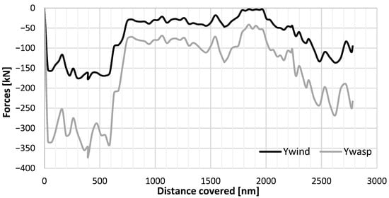
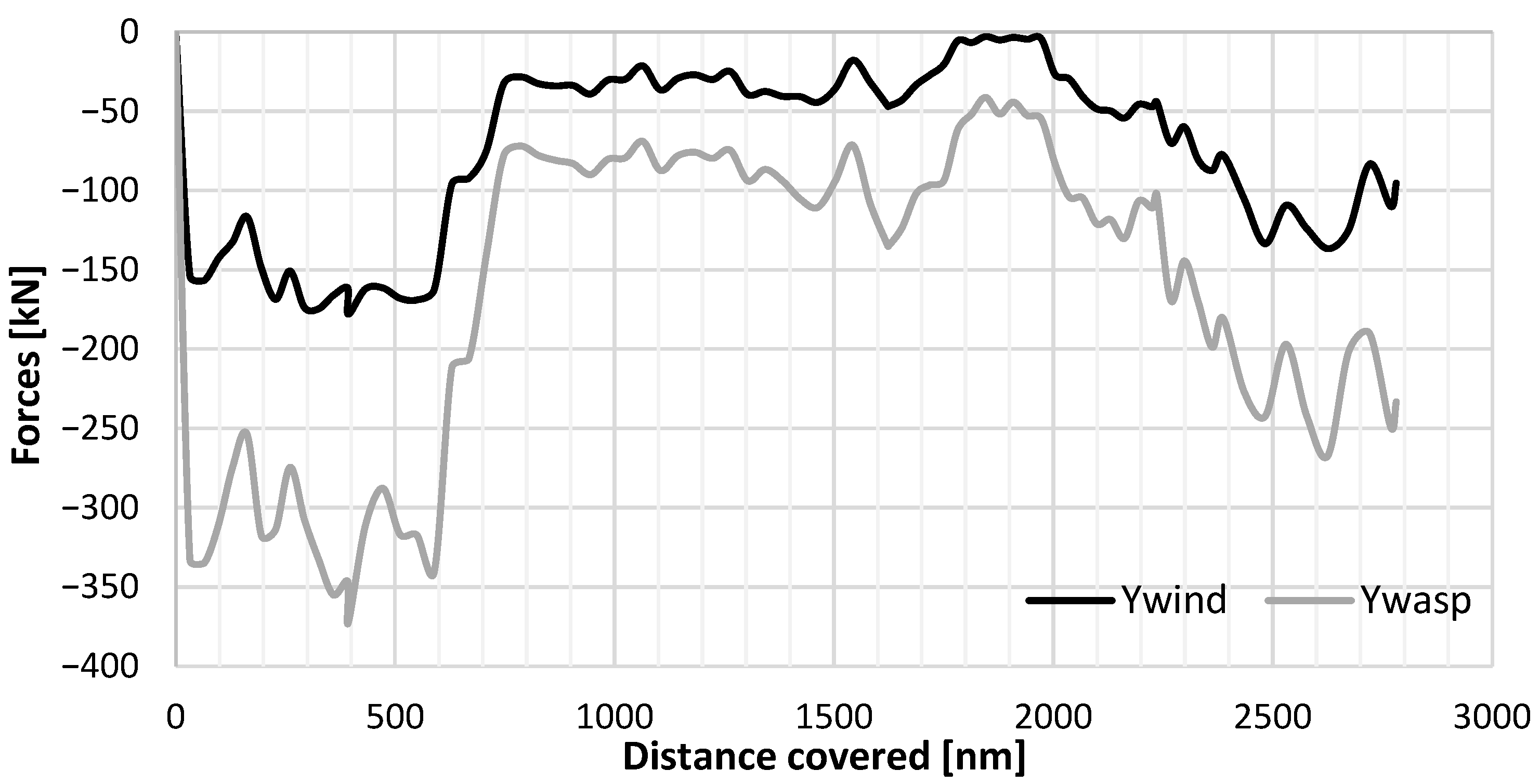
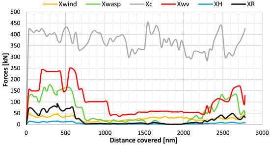
It is evident that high wind speeds prevailing during the first 500 nautical miles, combined with quarter-to-bow wind angles, lead to decreased ME power demands when the WASP system is installed, particularly when the 1-DOF model is considered. Under these conditions and when the 3-DOF model is used, the transverse forces generated by the wind and the WASP system are significant compared with all the longitudinal forces (Figure 12). In addition, the rudder resistance increases, as well as the longitudinal force from the WASP system (Figure 13).
Figure 12.
Transverse forces along the optimal path.
Figure 13.
Longitudinal forces along the optimal path.
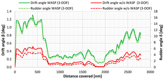
As illustrated in Figure 14, which presents data on induced drift and rudder angles, high rudder resistance values are also justified. The presence of the WASP system, on the exact same path, can even triple the induced rudder and drift angles at certain points along the trajectory, resulting in non-negligible additional forces, particularly from the rudder.
Figure 14.
Drift and rudder angles along the optimal route considering different scenarios.
5.3. Comparison Between the Optimal Routes Derived from the Two Ship Models
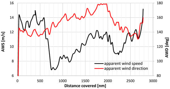
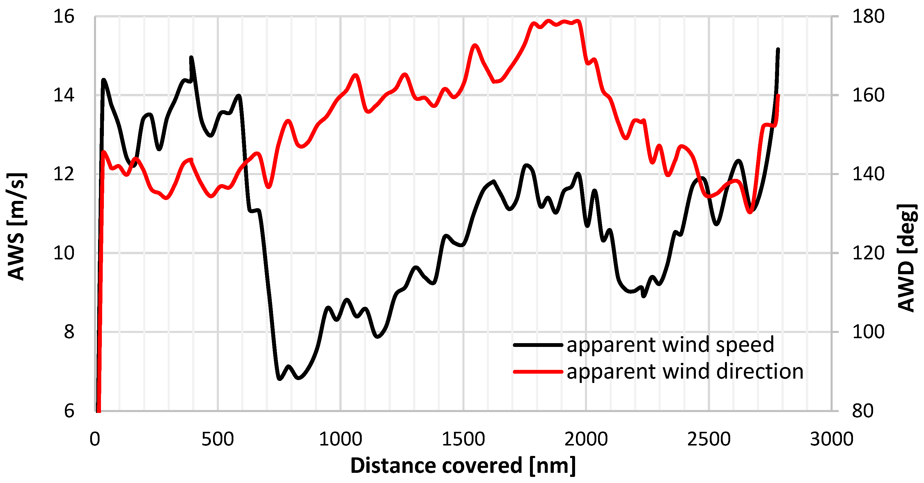
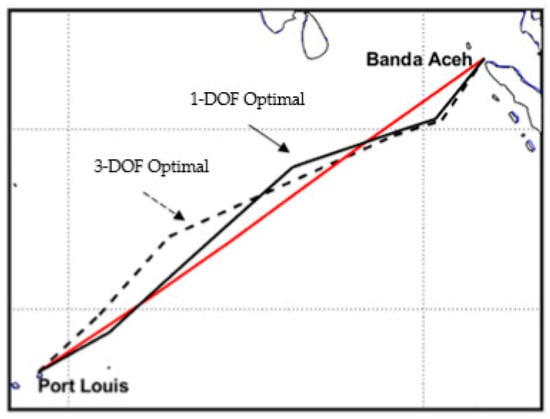
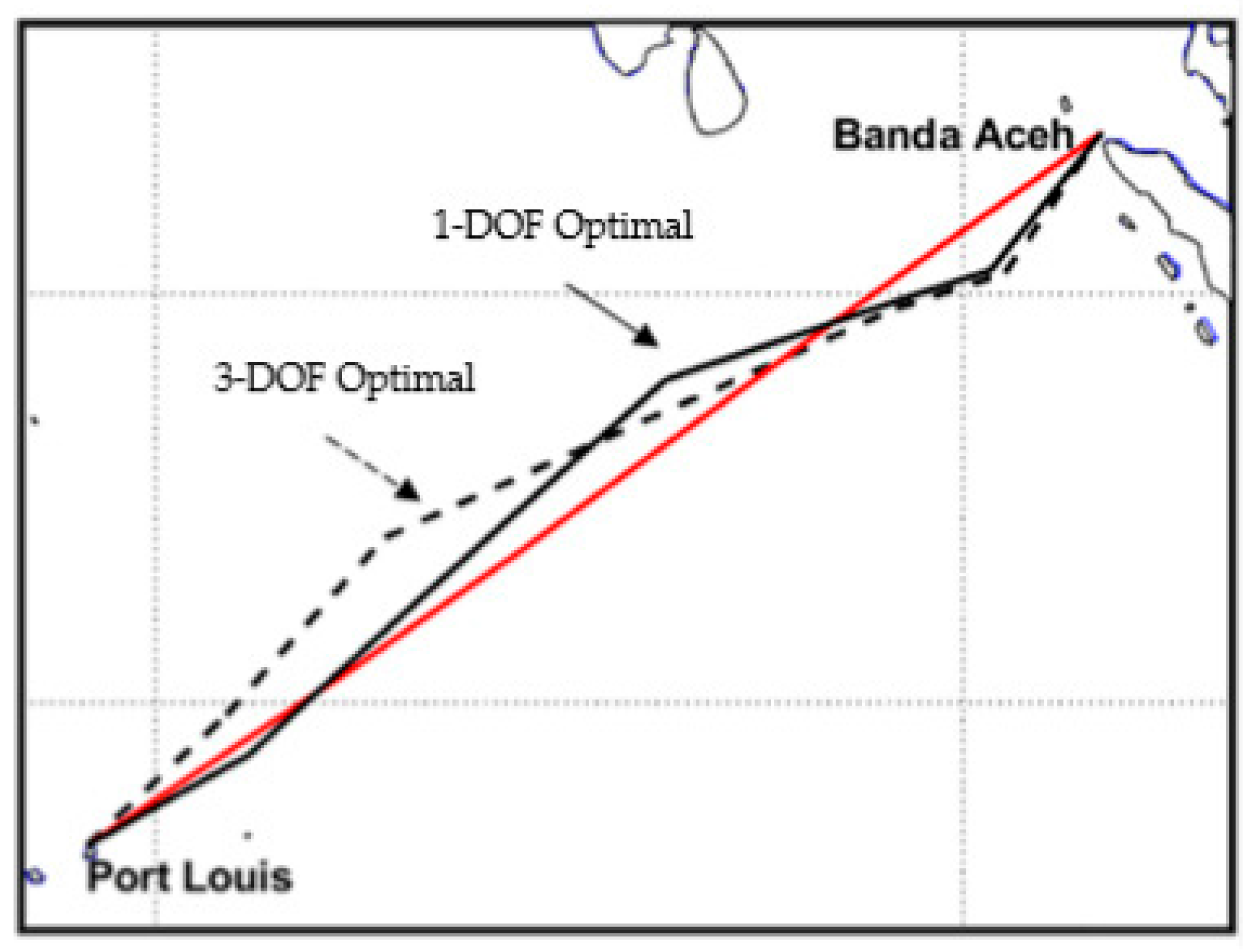
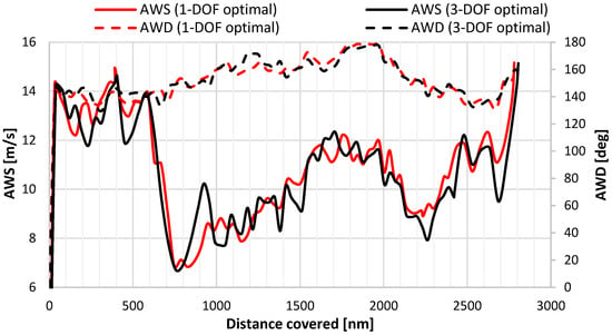
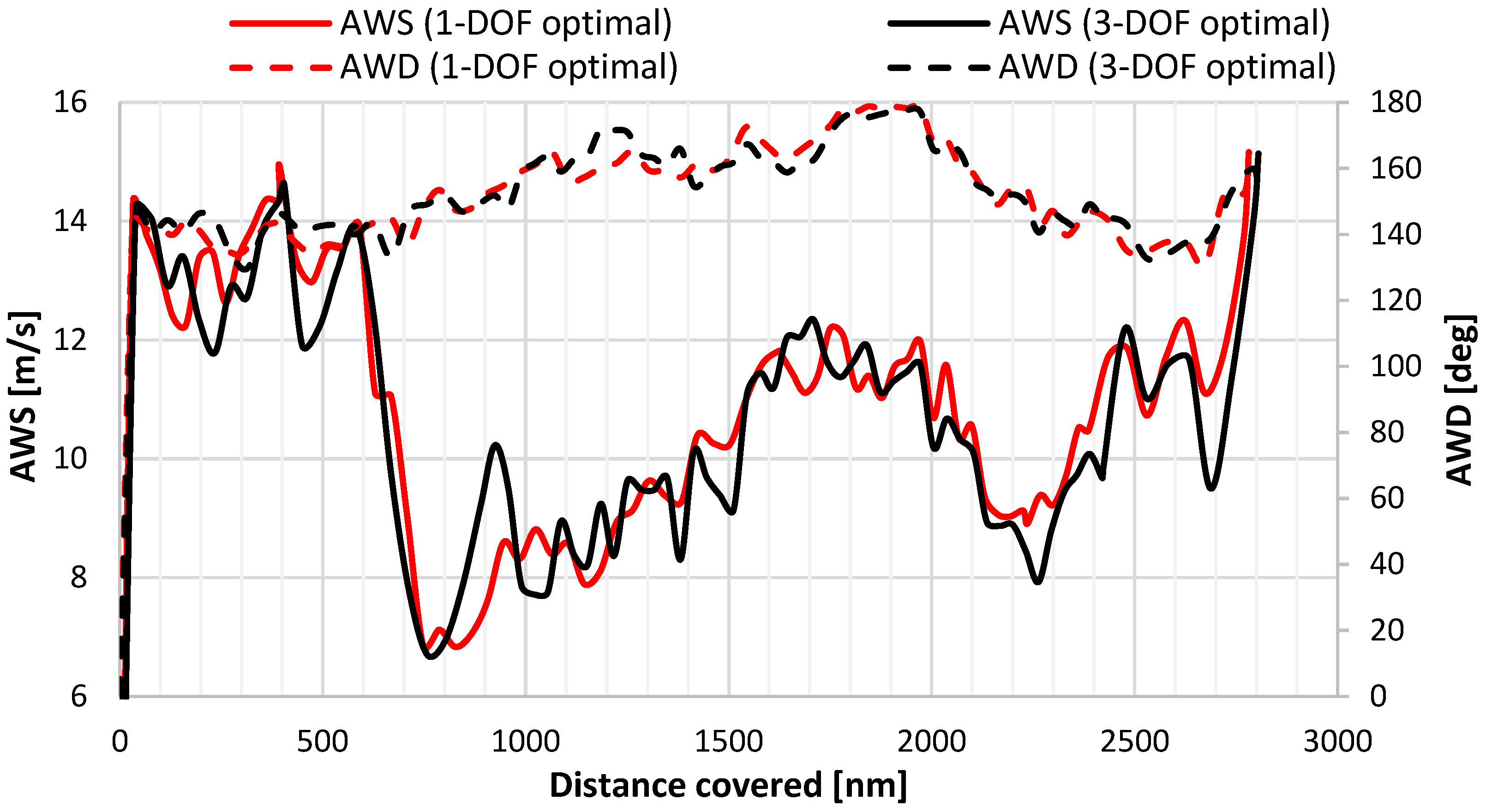
A new optimization has been conducted using the same genetic algorithm, considering the 3-DOF ship model. The settings of the optimization algorithm remain the same, as does the assumed vessel speed. In Figure 15 the optimal route considering the 3-DOF ship model is plotted on the map along with the real route and the optimal 1-DOF ship model. In addition, Figure 16 shows the apparent wind speed (AWS) and its direction (AWD) along the new optimal route and the prior one. The wind characteristics encountered for both optimal solutions are very similar in most parts of the trajectory. However, in certain regions, for example, along the very first 600 nm, the 3-DOF optimal path tends to favor slightly lower wind speeds. This seems to be a trade-off between maximizing the generated thrust from the WASP system but also limiting the generated side forces and yaw moments at the same time.
Figure 15.
Real voyage (red) and optimal routes found with 3-DOF and 1-DOF ship models when WASP is considered.
Figure 16.
Apparent wind speed and direction along the 3-DOF optimal route.
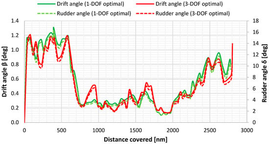
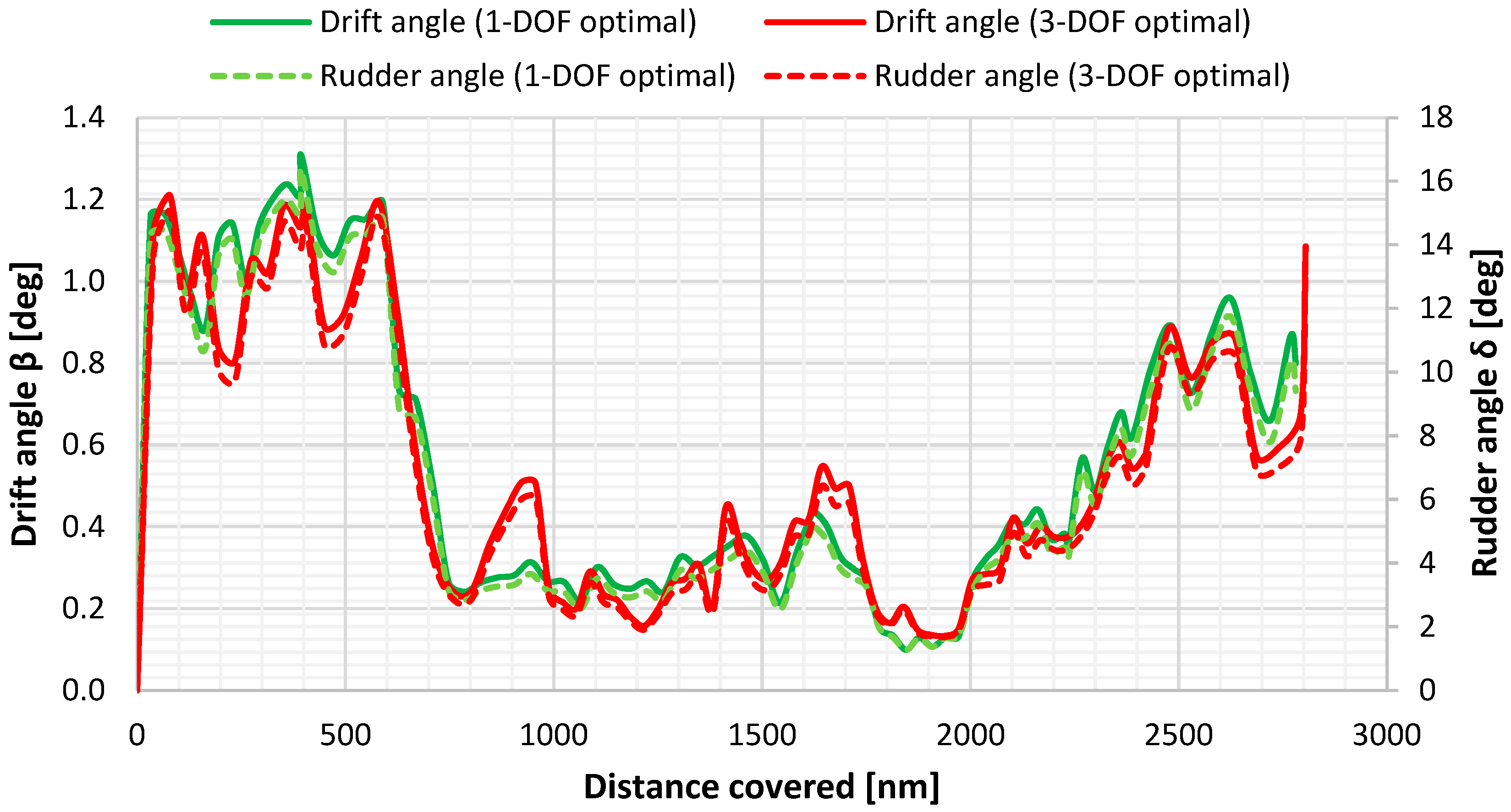
A notable point is the comparison between the newly obtained optimal solution (3-DOF ship model (optimal)) and the previously identified optimal route with the 1-DOF ship model, which highlights the compromises required to achieve a new optimal solution when using the 3-DOF ship model. In Figure 17, the drift and rudder angles are compared, showing that the algorithm seeks paths to maintain low rudder angles and consequently to keep the rudder resistance as low as possible (Figure 18).
Figure 17.
Drift and rudder angles along the 3-DOF- and 1-DOF-identified optimal paths.
Figure 18.
Longitudinal rudder forces along the 3-DOF- and 1-DOF-identified optimal paths.
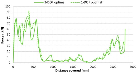
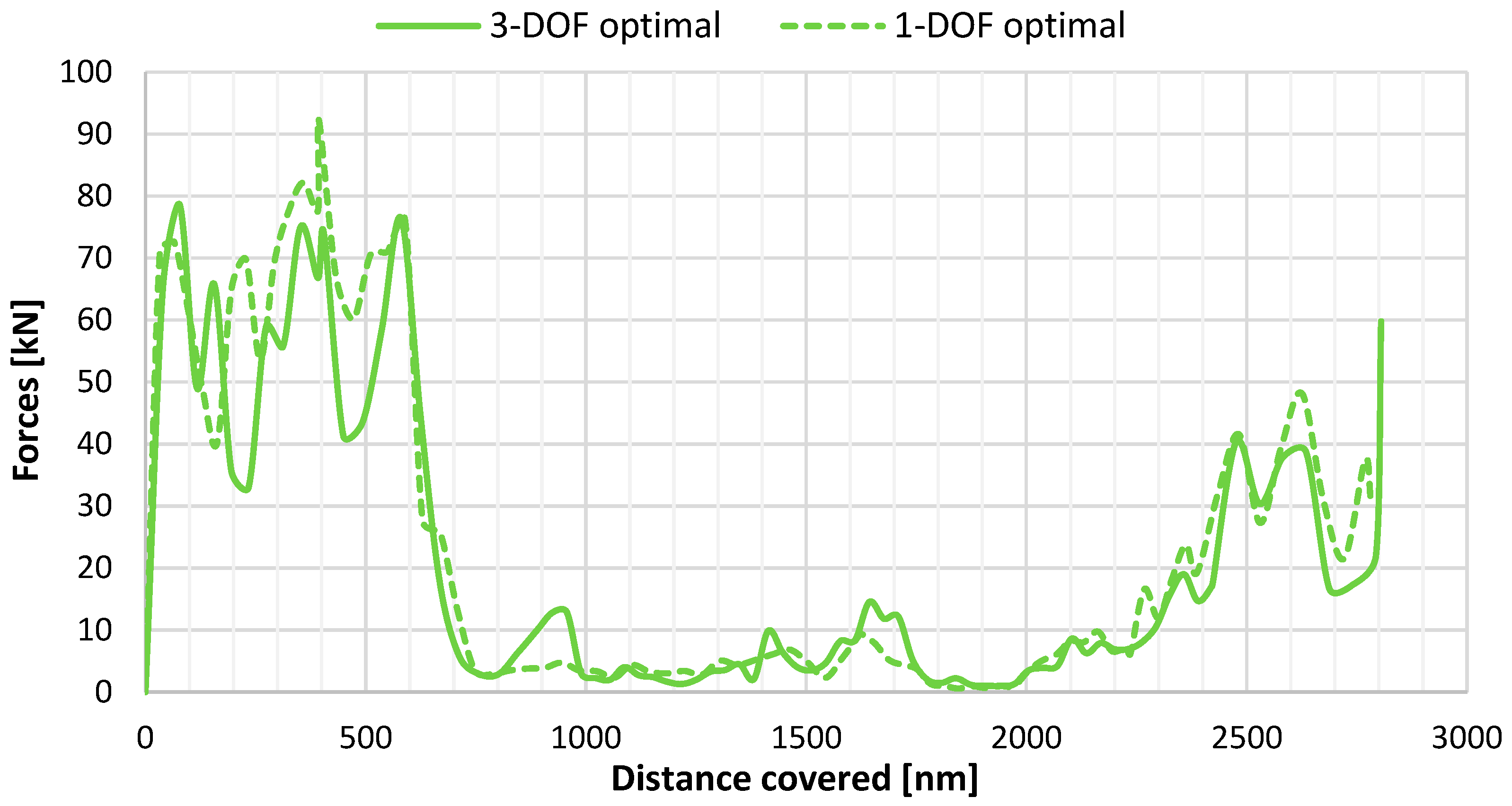
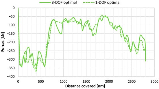
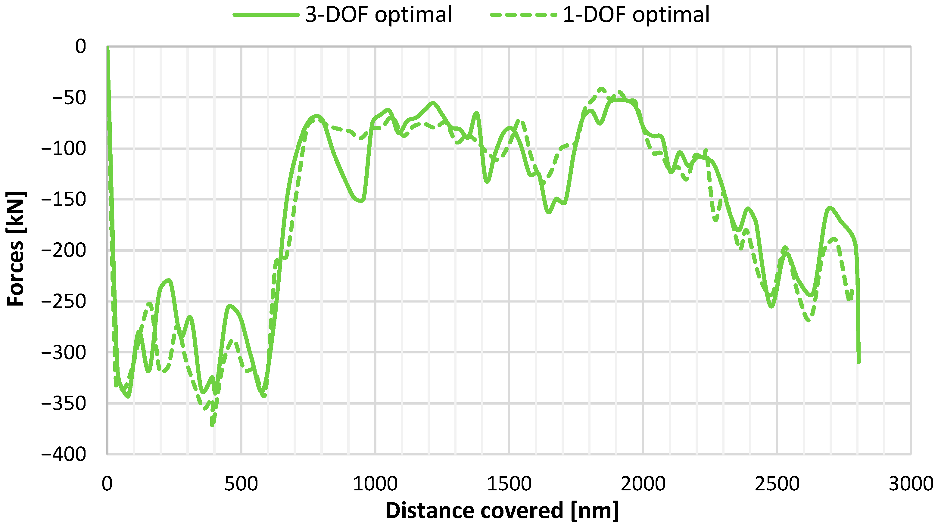
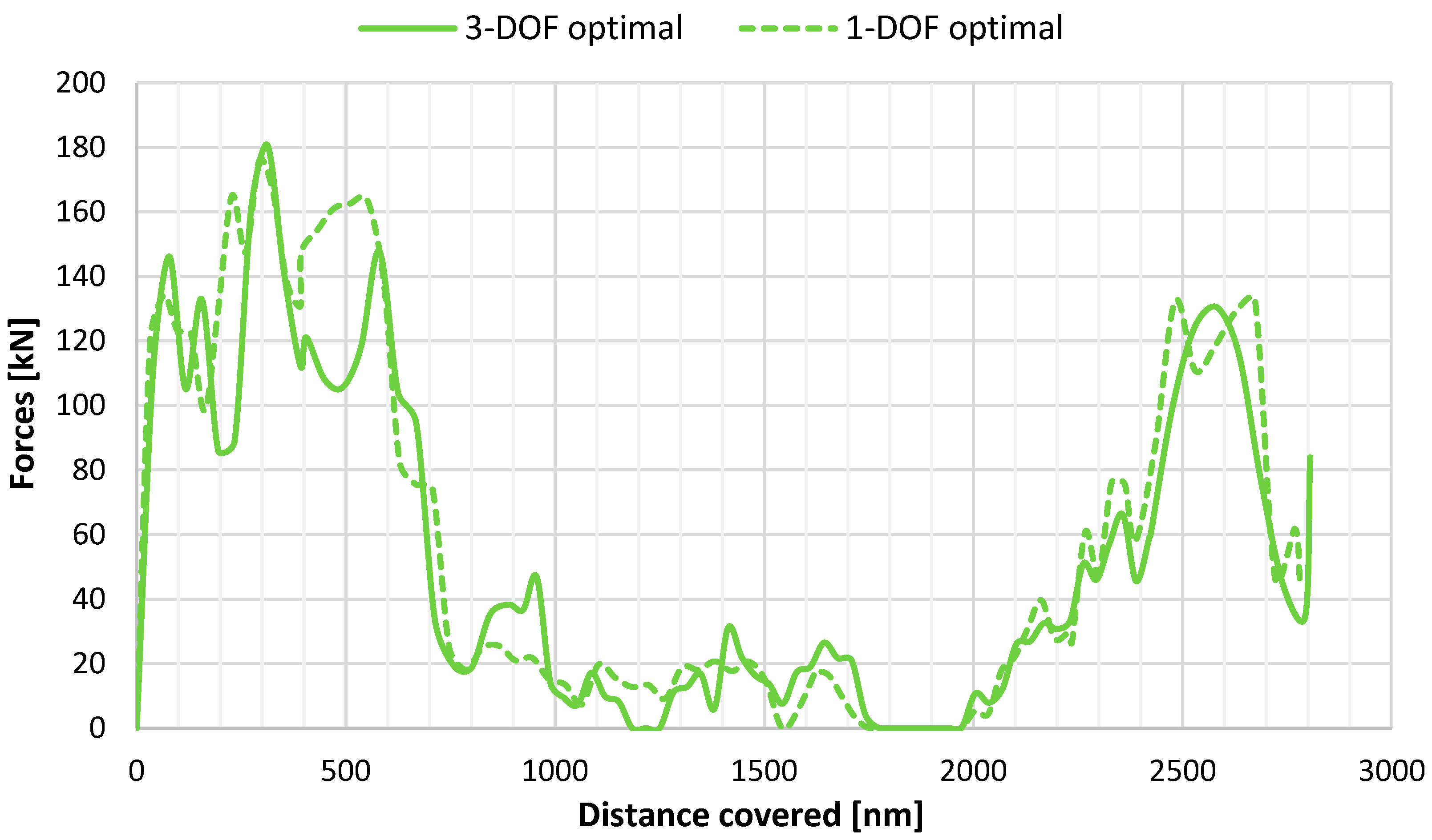
In Figure 19 and Figure 20, the transverse and the longitudinal forces from the WASP system are presented, respectively. A trade-off between the longitudinal and transverse force developed by the WASP system is needed so the optimal path will maximize the first one while keeping the second low to prevent the development of high rudder angles.
Figure 19.
Transverse WASP forces for the 3-DOF and 1-DOF optimal paths.
Figure 20.
Longitudinal WASP forces of the 3-DOF and 1-DOF optimal paths.
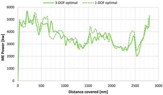
Moreover, the ME power for both optimal routes is plotted in Figure 21, showing that the new optimal solution achieves a slight decrease in demanded power. This decrease is not significant, primarily due to the prevailing wind conditions in the sea area under investigation. It is expected that, along trajectories with beam wind conditions and/or higher wind speeds, higher differences would arise.
Figure 21.
ME power along the 3-DOF and 1-DOF optimal paths.
The reduction in ME power is also reflected in ME FOC and presented in Table 4, which summarizes all the information for the evaluation of all routes tested when using both the 1-DOF and the 3-DOF model. FOC as a performance metric is selected for these results, as it serves as the objective function of the weather routing optimization. Furthermore, the table presents both the FOC of the ME and the DGs, highlighting the required power for such a system to operate, and thus it reports the combined contribution of the main engine and auxiliary power demand, capturing the overall energy impact of route selection and WASP operation. In addition, a key performance indicator (KPI) regarding the required FOC per total distance for each case is included to point out performance evaluation. Comparing the two models employed to evaluate the real voyage, negligible differences in FOC savings were observed when the WASP system is not considered, whereas the difference is about 6% when the WASP system is present. A similar trend is observed for the optimal solutions. The optimal path obtained using 1-DOF modelling and considering WASP installation indicates 12.95% fuel savings compared to the real voyage when no WASP system is installed. However, the same path performs slightly worse under the 3-DOF modelling, resulting in about 7% FOC reduction. The new optimization using the 3-DOF ship model resulted in a revised optimal trajectory, achieving an 8.32% FOC reduction and thus improving the savings. However, this optimal path requires about two more hours of travel (0.85%) than the optimal path found while using the 1-DOF modelling considering the same constant speed. According to Table 3, the optimal solution obtained from the 3-DOF ship model requires approximately 3 t less fuel oil than the optimal obtained from the 1-DOF Ship Model, as tested with the 3-DOF ship model. The new optimal trajectory achieves this reduction in FOC because it is formed in sea regions where the generated transverse forces of the WASP system remain lower, while, at the same time, the thrust from the WASP devices is almost preserved (Figure 19 and Figure 20).
Table 4.
Summary results for the examined routes using the 1-DOF and 3-DOF models.
6. Discussion
This study demonstrates the practical impact of using a WASP system (suction type) on a real route considering both 1- and 3-DOF modelling approaches. When the 3-DOF model is applied under the same prevailing conditions, the overall performance gain is reduced compared to the 1-DOF model; however, the net benefit of the WASP system remains clearly positive. The combined application of weather routing and WASP shows significant reductions in FOC, particularly when side forces and yaw moments are neglected. The optimal route obtained from the 1-DOF optimization was subsequently evaluated using the 3-DOF model and compared with the route optimized directly using the 3-DOF model. The 3-DOF optimal route achieved a slight additional improvement, mainly due to differences in the prevailing weather conditions.
More specifically, optimization based on the 3-DOF model identified an alternative optimal path, with noticeable improvements during the initial 600 nautical miles of the voyage, where lower wind speeds prevail. This outcome reflects a trade-off between maximizing thrust generation from the WASP system and limiting the associated side forces and yaw moments, highlighting added value introduced by the 3-DOF formulation.
However, both modeling approaches are based on empirical and semi-analytical formulations, and they thus provide a practical yet first-order estimate of WASP performance. It should be noted that these methods rely on simplifying assumptions that cannot fully capture the complex aerohydrodynamic interactions between individual sail units, as well as between the sails and the ship’s superstructure. In particular, aerodynamic interaction effects were neglected in the present study, as well as in our previous work [6], where side forces and yaw moments were not considered within the 1-DOF modeling framework. This simplification was intentionally adopted to ensure methodological consistency and allow for a direct comparison between the 1-DOF and 3-DOF approaches.
Nevertheless, aerodynamic interaction effects may influence the overall performance of wind-assisted propulsion systems when multiple sails are installed. For example, Tilling [13] investigated sail–sail and sail–ship interaction effects using high-fidelity CFD simulations, determining that mutual interference can significantly alter local flow fields and the resulting aerodynamic forces. Such findings highlight the importance of accounting for interaction effects in more advanced performance assessments.
Additionally, roll motion is neglected in the current study. This assumption is considered reasonable for the examined vessel, the relatively large size of which would result in limited roll amplitudes under typical operating conditions according to its stability booklet. Consequently, the influence of roll on the aerodynamic performance of the WASP systems and on the overall force balance is expected to be secondary compared to the sway and yaw motions.
The inclusion of sail–sail and sail–superstructure interaction effects is recognized as an important extension and will be addressed in future research to further enhance the accuracy of the performance assessment. Similarly, the extension to a 4-DOF model including roll motion represents a natural next step, particularly when examining smaller vessels where roll effects may be more pronounced. Finally, the integration of high-fidelity CFD simulations could be also employed to refine resistance predictions, especially for quantifying drift forces and rudder-induced losses, and thus to supplement the semi-empirical formulations utilized in the current study.
Another limitation of the present study is the lack of validation with experimental or CFD results of the developed performance prediction model. It should be noted, however, that the methodological approach proposed by Skogman was previously tested against experimental data for the drift and rudder angles in the work of Elger, where good agreement was reported. Moreover, as a first step toward the development of a more detailed performance model, our focus was on exploring the differences between the proposed 3-DOF formulation and the initial 1-DOF approach. Nevertheless, the importance of validating any performance prediction model is acknowledged. Accordingly, future research will focus on validating the proposed 3-DOF model. As an initial step, the utilization of short-term sea trials following ITTC procedures [5] could provide a quantitative assessment of the model’s accuracy and applicability, thereby strengthening its use for reliable performance prediction.
An additional point worthy of discussion concerns the impact of uncertainties related to weather forecasts and their propagation into route optimization outcomes, especially when the difference in FOC predictions between the modelling approaches is small. It should be noticed that such an examination was not explicitly quantified, as addressing such uncertainties would require dedicated studies, for example a stochastic or ensemble-based framework, which lies beyond the scope of this work, but it is recognized as a promising area for future research. However, since the present work focuses on a comparative evaluation of modelling approaches, identical weather inputs are applied to both the 1-DOF and 3-DOF frameworks. Consequently, uncertainties associated with weather forecasts are expected to influence both approaches in a comparable manner, thereby primarily affecting absolute performance metrics rather than the relative differences between models.
Larger gains are also expected to be observed in future studies when speed optimization will be part of the procedure. Incorporating speed management instead of maintaining a constant speed, as in the present study, could also lead to general improvements, as well as improving the performance of the WASP system. Routing through favorable regions (high wind speed combined with beam directions) would allow for an increase in vessel speed, enhancing the apparent wind experienced by the auxiliary propulsion system. Meanwhile, in unfavorable conditions, the system can maintain efficiency at some point due to the vessel’s slowing down.
Moreover, the issue of the realistic operational implementation of the developed framework shall be discussed. Notably, this study assumes idealized adherence to the optimized route and heading. In practice, deviations will definitely arise due to navigational constraints, safety considerations, and operator decisions. The investigation of on-board routing implementation, operator compliance, and the robustness of optimization results under realistic operational conditions is identified also as an important topic for future research.
7. Conclusions
The study investigated the impact of incorporating a 3-DOF model into the existing performance model of a weather routing tool, which explicitly accounts for Wind-Assisted Ship Propulsion Systems (WASP). The methodology proposed by Skogman [16] was embedded by solving algebraic relations regarding the calculation of the drift and rudder angles based on the balance of side forces and yaw moments, respectively. For weather routing purposes, this balance of forces and moments is appropriate, as well as being simpler and faster than time-domain 3-DOF modelling, where the focus is mostly on dynamic course keeping.
The reference ship is a Kamsarmax-type bulk carrier and the initial simulation results show that the 1-DOF model tends to overestimate fuel savings. Specifically, assuming 7.5 m/s true wind speed for a range of apparent wind directions, the 1-DOF model predicted up to 26% fuel savings, while the respective calculations using the 3-DOF model predicted FOC reductions up to 23.5%, with an average difference of 3.5%. Moreover, the results from a broader wind speed range reveal that higher wind speeds lead to greater divergence between the 1-DOF and 3-DOF models—up to 7% ME MCR—indicating that transverse effects play an increasingly significant role at elevated wind conditions.
The presented WASP system has also been tested on a past voyage of the reference ship, using both 1- and 3-DOF modelling, again highlighting the decrease in FOC savings when the more detailed approach is adopted, which accounts for both transverse forces and yaw moments. In cases where WASP is not considered, the two ship model approaches are almost identical. Obviously, this is not a general rule. During the tested period of time in the specific sea area of the voyage under investigation, the prevailing winds were relatively weak, and the apparent heading corresponds mainly to head winds. In cases where the WASP system is present, it was determined that the optimal path may vary when using the 1- or the 3-DOF model. When side forces and yaw moments are included, following a path optimized with a 1-DOF model can lead to unanticipated increase in FOC consumption. The analysis showed that the optimal route generated by the 3-DOF model yielded a 1.25% improvement in total FOC savings relative to the route optimized with the 1-DOF model when both were assessed using the 3-DOF formulation. Therefore, it was demonstrated how optimal routes obtained using 1-DOF formulations can change when 3-DOF effects are considered, highlighting a trade-off between maximizing thrust and limiting side forces and yaw moment.
Overall, the current study presents a modelling framework and comparative methodology that demonstrates the practical importance of including lateral aerodynamic effects when assessing WASP systems. The importance of including transverse forces and yaw moments is demonstrated, particularly in the presence of a WASP system. The 3-DOF formulation approach offers a more detailed and physically representative assessment of FOC savings for ships equipped with WASP systems. Weather routing optimization combined with the auxiliary thrust from WASP systems can help towards contribute to substantial reduction in FOC and significantly advance toward greener shipping.
Author Contributions
Conceptualization, A.K. and N.T.; methodology, A.K. and N.T.; software, A.K.; data curation, A.K. and N.T.; writing—original draft preparation, A.K. and N.T.; writing—review and editing, N.T.; supervision, N.T.; project administration, N.T.; funding acquisition, N.T. All authors have read and agreed to the published version of the manuscript.
Funding
The present work was supported by the Retrofit55 project (Retrofit solutions to achieve 55% GHG reduction by 2030), which has received funding from the European Union’s Horizon Europe Research and Innovation Program under Grant Agreement No. 101096068.
Data Availability Statement
The dataset generated during this study is available in Zenodo and can be accessed via the persistent identifier https://doi.org/10.5281/zenodo.17859015. This dataset is made available under the license: Creative Commons Attribution 4.0 International License (CC-BY 4.0). For additional inquiries regarding the dataset, please contact the corresponding author.
Acknowledgments
The authors would especially like to thank Laskaridis Shipping Co. Ltd. and Bound 4 Blue S.L. for the productive conversations and for sharing initial design ship and WASP system data within the framework of the Retrofit55 project.
Conflicts of Interest
The authors declare no conflicts of interest.
Nomenclature
| AL | Lateral windage area |
| Ar | Rudder area |
| ARh | Effective hull aspect ratio |
| ARr | Effective rudder aspect ratio |
| ARr,geo | Geometric rudder aspect ratio |
| BWL | Waterline beam |
| cB | Block coefficient |
| cmean | Mean rudder chord |
| cN | Aerodynamic yaw moment coefficient |
| cXD | Added resistance coefficient due to drift |
| cY | Aerodynamic lateral force coefficient |
| FN | Rudder normal force |
| LOA | Overall length |
| LWL | Waterline length |
| n | Propeller/engine revolutions |
| NH | Hydrodynamic yaw moment |
| NR | Rudder induced yaw moment |
| Nwasp | Yaw moment generated by WASP |
| Nwind | Aerodynamic yaw moment due to wind |
| PB | Main Engine brake power |
| T | Draft |
| u | Ship speed in x-direction |
| VAW | Apparent wind speed |
| Vr | Rudder inflow velocity |
| VS | Ship speed |
| Vtw | True wind speed |
| w | Wake fraction |
| x1, x2, x3, x5 | Rudder geometric parameters |
| Xc | Calm water resistance |
| XH | Added resistance due to drift/Hydrodynamic longitudinal force |
| XP | Propeller thrust |
| XR | Rudder induced added resistance |
| xR | Longitudinal rudder lever arm |
| xs | Longitudinal location of WASP force |
| Xwasp | WASP induced thrust |
| Xwind | Aerodynamic wind resistance |
| Xwv | Added wave resistance |
| YH | Hydrodynamic lateral force |
| Ym0 | Auxiliary parameter in drift equation |
| YR | Rudder lateral force |
| Ywasp | Lateral force generated by WASP |
| Ywind | Aerodynamic lateral force due to wind |
| Hydrodynamic derivatives of the lateral force | |
| Hull force factor due to rudder | |
| Rudder inflow angle | |
| β | Drift angle |
| δ | Rudder angle |
| ρ | Air density |
| ρw | Water density |
| φ | Apparent wind angle |
| Ship speed in y-direction | |
| ’ | Dimensionless sway velocity |
Abbreviations
| ACP | Aerodynamic Center of Pressure |
| AWD | Apparent Wind Direction |
| AWS | Apparent Wind Speed |
| CFD | Computational Fluid Dynamics |
| CLR | Center of Lateral Resistance |
| CMEMS | Copernicus Marine Environment Monitoring Service |
| CPP | Controllable Pitch Propeller |
| DG | Diesel Generator |
| DOF | Degrees of Freedom |
| DWT | Deadweight Tonnage |
| FOC | Fuel Oil Consumption |
| GA | Genetic Algorithm |
| IMO | International Maritime Organization |
| ITTC | International Towing Tank Conference |
| JONSWAP | Joint North Sea Wave Project (wave spectrum) |
| KPI | Key Performance Indicator |
| MCR | Maximum Continuous Rating |
| ME | Main Engine |
| ME FOC | Main Engine Fuel Oil Consumption |
| NTUA | National Technical University of Athens |
| Ro-Ro | Roll-on/Roll-off |
| RPM | Revolutions Per Minute |
| SFOC | Specific Fuel Oil Consumption |
| VLCC | Very Large Crude Carrier |
| WASP | Wind Assisted Ship Propulsion |
| WPS | Wind Propulsion Systems |
References
- IMO. Strategy on Reduction of GHG Emissions from Ships; Resolution MEPC.377(80); IMO: London, UK, 2023.
- European Maritime Safety Agency. Potential of Wind-Assisted Propulsion for Shipping; EMSA: Lisbon, Portugal, 2023.
- International Maritime Organization. MEPC 81/INF.39, Reduction of GHG Emissions from Ships: White Paper on Wind Propulsion; International Maritime Organization: London, UK, 2024.
- Alterskjær, S.A.; Eggers, R.; Gao, Y.; Kim, Y.; Kume, K.; Trodden, D.; Werner, S.; Zhang, X. Predicting the Power Saving of Wind Powered Ships; ITTC Recommended Procedures and Guidelines, Document 7.5-02-03-01.9, Rev. 00; International Towing Tank Conference: Hobart, Australia, 2024. [Google Scholar]
- International Towing Tank Conference. Sea Trials for Assessing the Power Saving from Wind Assisted Propulsion; ITTC Recommended Procedures and Guidelines, Procedure, Document 7.5-04-01-02, Rev. Draft 3.3; International Towing Tank Conference: Hobart, Australia, 2024. [Google Scholar]
- Themelis, N.; Kytariolou, A.; Baranda, S.J.C.; Saettone, S.; Tsoulakos, N. Integrating WASP Technology with Optimal Weather Routing for Enhanced Navigation. In Innovations in Sustainable Maritime Technology—IMAM 2025; Spyrou, K.J., Themelis, N., Eds.; Springer: Cham, Switzerland, 2025. [Google Scholar] [CrossRef] [Scilit]
- Bentin, M.; Zastrau, D.; Schlaak, M.; Freye, D.; Elsner, R.; Kotzur, S. A new routing optimization tool-influence of wind and waves on fuel consumption of ships with and without wind assisted ship propulsion systems. Transp. Res. Procedia 2016, 14, 153–162. [Google Scholar] [CrossRef] [Scilit]
- Viola, I.M.; Sacher, M.; Xu, J.; Wang, F. A numerical method for the design of ships with wind-assisted propulsion. Ocean Eng. 2015, 105, 33–42. [Google Scholar] [CrossRef] [Scilit]
- Ammar, S.; Seddiek, I. Wind-assisted propulsion system onboard ships: Case study of Flettner rotors. J. Mar. Sci. Appl. 2021, 20, 45–59. [Google Scholar] [CrossRef] [Scilit]
- Vigna, A.; Figari, M. Wind-Assisted Ship Propulsion: Matching Flettner Rotors with Diesel Engines and Controllable Pitch Propellers. J. Mar. Sci. Eng. 2023, 11, 1072. [Google Scholar] [CrossRef] [Scilit]
- Van der Kolk, E.; Visonneau, M.; van Terwisga, T. Hydrodynamic forces and moments acting on ships at leeway angles: Experimental and numerical investigation. Ocean Eng. 2019, 180, 332–348. [Google Scholar] [CrossRef] [Scilit]
- Tillig, F.; Ringsberg, J. A 4 DOF simulation model developed for fuel consumption prediction of ships at sea. Ships Offshore Struct. 2019, 14, 112–120. [Google Scholar] [CrossRef] [Scilit]
- Tillig, F.; Ringsberg, J.W. Design, operation and analysis of wind-assisted cargo ships. Ocean Eng. 2020, 211, 107603. [Google Scholar] [CrossRef] [Scilit]
- Ma, R.; Wang, Z.; Wang, K.; Zhao, H.; Jiang, B.; Liu, Y.; Xing, H.; Huang, L. Evaluation Method for Energy Saving of Sail-Assisted Ship Based on Wind Resource Analysis of Typical Route. J. Mar. Sci. Eng. 2023, 11, 789. [Google Scholar] [CrossRef] [Scilit]
- Ghorbani, M.; Slaets, P.; Lacely, J. A numerical simulation tool for a wind-assisted vessel verified with logged data at sea. Ocean Eng. 2023, 290, 116319. [Google Scholar] [CrossRef] [Scilit]
- Skogman, A. The practical meaning of lateral balance for a sail-assisted research vessel. J. Wind Eng. Ind. Aerodyn. 1985, 20, 201–226. [Google Scholar] [CrossRef] [Scilit]
- Inoue, S.; Hirano, M.; Kijima, K. Hydrodynamic derivatives on ship maneuvering. Int. Shipbuild. Prog. 1981, 28, 112–125. [Google Scholar] [CrossRef] [Scilit]
- Elger, D.E.; Bentin, M.; Vahs, M. Comparison of different methods for predicting the drift angle and rudder resistance by wind propulsion systems on ships. Ocean Eng. 2020, 217, 108152. [Google Scholar] [CrossRef] [Scilit]
- Marie, S.; Courteille, E. Sail-assisted motor vessels weather routing using a fuzzy logic model. J. Mar. Sci. Technol. 2014, 19, 265–279. [Google Scholar] [CrossRef] [Scilit]
- Reche-Vilanova, M.; Bingham, H.B.; Fluck, M.; Morris, D.; Psaraftis, H.N. Cost–benefit analysis and design optimization of wind propulsion systems for a tanker retrofit case. Marit. Transp. Res. 2025, 8, 100132. [Google Scholar] [CrossRef] [Scilit]
- Kytariolou, A.; Themelis, N. Optimized route planning under the effect of hull and propeller fouling and considering ocean currents. J. Mar. Sci. Eng. 2023, 11, 828. [Google Scholar] [CrossRef] [Scilit]
- Kytariolou, A.; Themelis, N. Ship routing optimization based on forecasted weather data and considering safety criteria. J. Navig. 2022, 75, 1310–1331. [Google Scholar] [CrossRef] [Scilit]
- International Towing Tank Conference (ITTC). Recommended Procedures and Guidelines: Analysis of Speed/Power Trial Data; International Towing Tank Conference (ITTC): Hobart, Australia, 2014. [Google Scholar]
- Liu, S.; Papanikolaou, A. Regression analysis of experimental data for added resistance in waves of arbitrary heading and development of a semi-empirical formula. Ocean Eng. 2020, 206, 107357. [Google Scholar] [CrossRef] [Scilit]
- Blendermann, W. Parameter identification of wind loads on ships. J. Wind Eng. Ind. Aerodyn. 1994, 51, 339–351. [Google Scholar] [CrossRef] [Scilit]
- MathWorks. Global Optimization Toolbox User’s Guide; The MathWorks, Inc.: Natick, MA, USA, 2022. [Google Scholar]

Disclaimer/Publisher’s Note: The statements, opinions and data contained in all publications are solely those of the individual author(s) and contributor(s) and not of MDPI and/or the editor(s). MDPI and/or the editor(s) disclaim responsibility for any injury to people or property resulting from any ideas, methods, instructions or products referred to in the content. |
© 2026 by the authors. Licensee MDPI, Basel, Switzerland. This article is an open access article distributed under the terms and conditions of the Creative Commons Attribution (CC BY) license.