


Abstract
Cross-well lithology recognition is important for reservoir characterization, but its application to newly drilled wells is constrained by inter-well variations in logging responses and limited lithological labels. This study proposes a geoscience knowledge-guided machine-learning method for lithology recognition under limited target-well labels. Geochemical indicators and conventional logging data are combined to construct geologically interpretable features, while few-shot transfer learning is used to reduce class imbalance and inter-well distribution differences. Geological knowledge is introduced as probabilistic constraints and integrated with model predictions through uncertainty-aware fusion. The method is evaluated using volcanic reservoir well-logging data from the Pearl River Mouth Basin. Three representative wells are used as the source domain and an independent newly drilled well as the target domain, with three labeled samples per lithology class used for adaptation and the remaining samples for independent testing. Repeated experiments with 10 random seeds yield an accuracy of 88.03% ± 6.09%, with improved classification performance and lower variability than the compared baseline methods. The results show that combining geological knowledge with few-shot learning can improve the robustness of cross-well lithology recognition and provide a practical approach for lithology prediction in heterogeneous volcanic reservoirs.
1. Introduction
Lithology identification is a fundamental component of reservoir characterization and plays an important role in hydrocarbon exploration, reservoir evaluation, and geological modeling [1,2]. Accurate lithological interpretation from well logging data provides essential information for reservoir prediction, drilling decision-making, and resource development [3,4]. However, in offshore volcanic reservoirs, such as those in the Pearl River Mouth Basin, complex volcanic activities, rapid facies variations, and strong heterogeneity result in considerable differences in mineral composition and logging responses, making conventional lithology interpretation challenging.
With the development of artificial intelligence, machine learning methods have been increasingly applied to automated lithology recognition from well logging data. Algorithms such as Random Forest (RF), Support Vector Machine (SVM), Artificial Neural Networks (ANN), and Gradient Boosting Decision Trees (GBDT) have shown advantages in capturing nonlinear relationships between logging responses and lithological categories [5,6,7,8]. Deep learning approaches have further improved feature representation capability by automatically extracting high-level patterns from large-scale datasets [5,9]. However, most existing data-driven methods rely on sufficient labeled samples and assume that training and testing datasets share similar feature distributions [10,11], which limits their applicability in practical geological scenarios.
In actual exploration and development, these assumptions are often difficult to satisfy. Due to variations in depositional environment, volcanic evolution, diagenesis, drilling conditions, and measurement processes, logging responses may exhibit considerable distribution differences among wells. Such inter-well distribution discrepancies, commonly referred to as domain shift, can substantially degrade the performance of models trained from existing wells when applied to newly drilled wells [4,12]. Meanwhile, obtaining sufficient lithological labels in new wells remains difficult because core sampling and laboratory analysis are expensive and limited. Therefore, developing reliable lithology recognition methods under cross-well and limited-label conditions remains a critical challenge.
Transfer learning provides an effective strategy to address the problem of insufficient labeled samples by transferring knowledge from data-rich source wells to target wells [13]. Recent studies have explored domain adaptation, adversarial learning, and meta-learning approaches to improve cross-well lithology prediction [14]. However, most existing transfer learning methods mainly focus on reducing statistical distribution differences between domains, while geological information related to mineral composition, lithogenesis, and geochemical evolution is rarely incorporated into the learning process [15]. As a result, purely data-driven models may suffer from limited geological interpretability and produce predictions inconsistent with geological constraints, particularly in highly heterogeneous volcanic reservoirs.
Geoscientific knowledge provides important prior information for understanding lithological formation and evolution processes. Integrating geological knowledge with machine learning models has recently attracted increasing attention in geoscience artificial intelligence [16]. Nevertheless, how to effectively incorporate geological constraints into cross-well lithology recognition while simultaneously addressing limited labeled samples and inter-well distribution discrepancies remains unresolved.
To address these challenges, this study proposes a geoscience knowledge-guided few-shot transfer learning framework for cross-well lithology recognition in complex volcanic reservoirs. The proposed framework integrates geological knowledge and data-driven learning throughout the recognition process. Geologically meaningful features are first constructed from geochemical indicators and conventional logging parameters to enhance lithological discrimination. Subsequently, a few-shot transfer learning strategy incorporating sample balancing and feature distribution alignment is developed to reduce class imbalance and inter-well distribution discrepancies. Furthermore, geological knowledge is represented as probabilistic soft constraints and adaptively fused with machine learning predictions through an uncertainty-aware mechanism, improving prediction reliability and interpretability. The proposed framework is evaluated using volcanic reservoir logging datasets from the Pearl River Mouth Basin.
The main contributions of this study are summarized as follows:
- (1)
- A geoscience knowledge-guided few-shot learning framework is developed for cross-well lithology recognition under limited labeled-data conditions, linking previously characterized wells with the source domain and a newly drilled well with the target domain.
- (2)
- Geoscience-derived features are combined with conventional logging data, and few-shot target-well adaptation is used to reduce class imbalance and inter-well distribution differences.
- (3)
- Geological knowledge is introduced as probabilistic soft constraints and integrated with machine-learning predictions through uncertainty-aware fusion, avoiding rigid lithological classification rules.
- (4)
- The proposed method is evaluated on volcanic reservoir well-logging data from the Pearl River Mouth Basin through comparative, ablation, and sensitivity experiments under a few-shot target-domain setting.
The remainder of this paper is organized as follows. Section 2 reviews related studies. Section 3 describes the proposed methodology. Section 4 presents the results and discussion, including ablation, sensitivity, geological constraint, and comparative analyses. Section 5 summarizes the conclusions and discusses the limitations and future research directions.
2. Related Work
Machine learning has been widely used for lithology identification from well logs. Conventional methods, including random forest and support vector machines, have been applied to this task [6,7], followed by the use of deep learning models for automatic feature extraction from logging data [5,9]. However, a model trained with data from one or several wells may not perform equally well in a newly drilled well. Differences in geological conditions and logging practices can result in changes in logging responses between wells [4]. This problem is especially important for volcanic reservoirs in the Pearl River Mouth Basin, where lithological and geological heterogeneity can lead to complex logging and geochemical responses [17,18].
Transfer learning has therefore been introduced into cross-well lithology recognition. Its main purpose is to transfer information from labeled source wells to a target well with different data distributions [10,11]. Several approaches have been investigated, including transfer component analysis and CORAL for feature alignment [19,20], as well as adversarial, data-drift-aware, and similarity-based transfer methods [4,14,21,22]. Partial domain adaptation has also been considered when the target well contains only part of the lithology classes present in the source domain [23]. Most of these studies focus on reducing statistical differences between source and target data. The role of geological knowledge in this process has received less attention.
The limited availability of target-well labels has also motivated the use of few-shot and meta-learning methods. Prototypical Networks are commonly used for few-shot classification [24], and recent studies have combined meta-learning with Vision Transformers, semi-supervised learning, and graph-based methods for lithology recognition [25,26,27,28]. Few-shot learning has also been combined with geological knowledge for interwell stratigraphic correlation [29]. These studies show the potential of learning from a small number of target-domain samples, but the resulting predictions still depend mainly on the learned features and the source-domain data.
In this study, geological knowledge is introduced into the cross-well lithology recognition process in two ways. First, geochemical relationships are used to construct interpretable features together with conventional logging parameters. Second, geological information is expressed as probabilistic constraints and combined with machine-learning predictions using an uncertainty-aware fusion strategy. The method also uses a small number of labeled samples from the target well for adaptation. In this way, both target-well information and geological knowledge are considered in the recognition of lithologies across wells.
3. Materials and Methods
3.1. Study Area and Geological Setting
The study area is located in the Qionghai Uplift and its surrounding areas in the Pearl River Mouth Basin (PRMB), along the northern continental shelf of the South China Sea. The PRMB is one of the major offshore petroliferous basins in China. Influenced by multiple stages of tectonic deformation, magmatic activity, and sedimentary evolution, the basin contains diverse igneous rocks with complex spatial distributions. The Qionghai Uplift is located in the western part of the Zhu III Depression. It is bounded to the north by the Zhu 3-2 Fault and is adjacent to the Qionghai Sag. To the south, it connects with the Wenchang B Sag along the northern flank of the Shenhu Uplift, while it gradually plunges eastward into the Wenchang A Sag. The uplift generally extends in the NEE direction and exhibits a west-high and east-low structural configuration (Figure 1) [30,31,32,33].
Figure 1.
Areal distribution of volcanic reservoirs in the Qionghai Uplift and its surrounding areas, Pearl River Mouth Basin. Modified from Li et al. [33].
During the Jurassic–Cretaceous Yanshanian tectonic period, the Qionghai Uplift experienced several stages of compression and extension accompanied by magmatic activity. Volcanic eruptions and magmatic intrusions, followed by uplift and denudation, resulted in widespread Mesozoic igneous rocks and the development of volcanic and intrusive rocks in the buried-hill basement [17,18]. During the Cenozoic, the tectonic regime changed from compression to extension, followed by rifting and post-rift subsidence. Early reverse faults were reactivated as normal faults, forming fault-controlled rift structures [32]. Subsequent thermal subsidence was accompanied by increasing Neogene sedimentary cover [5,30].
The Mesozoic igneous rocks in the study area include volcanic and intrusive rocks. The volcanic rocks mainly comprise rhyolite, dacite, andesite, volcanic breccia, and tuff, while the intrusive rocks include granite and diorite. Their distribution is closely related to regional faults and magmatic activity (Figure 1). Rhyolite and tuff are relatively widespread, whereas andesite, volcanic breccia, granite, and diorite are more locally distributed. These different volcanic and intrusive assemblages result in variable lithological and logging responses within the buried-hill formations.
Three representative wells, XX-1, XX-2, and XX-3, were selected for this study. All three wells penetrate Mesozoic igneous basement rocks, with the major identified lithologies including tuff, dacite, rhyolite, diorite, and granite. As shown in Figure 2, the three wells exhibit different lithological assemblages and vertical distributions. Moreover, the same lithology may exhibit different natural gamma-ray and resistivity responses among wells, indicating pronounced inter-well variations in the geological and petrophysical characteristics of the igneous formations.
Figure 2.
Cross-sectional diagram of the three drilled wells in the study area.
The geological complexity of the study area is further reflected in the mineralogical and petrographic characteristics of the different lithologies. Representative cuttings were examined by thin-section analysis, as shown in Figure 3. Tuff exhibits a typical tuffaceous texture with volcanic and crystal fragments, whereas rhyolite shows a porphyritic texture. Dacite is mainly characterized by plagioclase phenocrysts, while diorite is dominated by plagioclase with minor quartz. These differences in texture and mineral composition provide direct petrographic evidence for distinguishing the major lithological types and support the geological reliability of the lithological interpretations used in this study.
Figure 3.
Thin-section photomicrographs of representative lithologies and their characteristic mineral assemblages.
It should also be noted that some lithologies exhibit partially overlapping geochemical compositions. For example, granite and rhyolite are both felsic igneous rocks and may therefore show similar elemental characteristics. Consequently, individual geochemical indicators are not used as independent lithology classification criteria. Instead, the geochemical information is incorporated as geological knowledge for subsequent feature construction and probabilistic geological constraints.
3.2. Data Description and Inter-Well Distribution Analysis
The dataset was constructed by integrating well-logging measurements, cuttings logging, sidewall core observations, and X-ray fluorescence (XRF) geochemical analyses from the studied wells. The available logging data include natural gamma ray, spectral gamma ray, resistivity, acoustic, porosity, elemental, photoelectric absorption, and density measurements, providing complementary information on the radioactive, elastic, electrical, petrophysical, and elemental characteristics of the formations. Figure 4 presents the integrated logging and cuttings-logging responses of well XX-2 and illustrates the main types of measurements used in this study.
Figure 4.
Integrated logging and cuttings-logging responses of well XX-2.
Cuttings-logging interpretations were used to establish the depth-matched lithological labels for supervised learning. In addition, 105 sidewall core samples were collected from the three wells and used as direct geological evidence for lithological interpretation. XRF analysis of drilling cuttings provided multi-element geochemical information, including Al, Ca, Fe, K, Na, Si, and other elements, which was used to characterize the elemental composition of different lithologies and to construct geologically interpretable features and geological constraints.
For the cross-well experiments, the data from XX-1, XX-2, and XX-3 were jointly combined to form the source domain, rather than being treated as three independent source domains. The source domain can therefore be expressed as
An independent fourth well was used as the target domain. The two domains differ in both lithological composition and feature distributions. As shown in Figure 5, the source domain contains seven lithology classes: mudstone, fine sandstone, tuff, diorite, dacite, granite, and rhyolite. The target domain contains three classes: mudstone, fine sandstone, and rhyolite. The source and target domains contain 608 and 70 labeled samples, respectively. Among the source samples, 479 belong to lithology classes not present in the target domain, accounting for approximately 78.8% of the source data. This difference indicates a clear mismatch in the label spaces of the two domains and reflects the limited lithological information commonly available in newly drilled wells.
Figure 5.
Lithological sample distributions in the source and target domains.
The feature distributions were further examined using principal component analysis (PCA). PCA was applied to the input features and used to project them into a two-dimensional space. As shown in Figure 6, PC1 and PC2 explain 24.9% and 18.4% of the total variance, respectively. The source-domain samples from XX-1, XX-2, and XX-3 are shown as open markers, while samples from the independent target well are shown as filled markers. The two domains occupy different regions of the PCA space, although some overlap is present, indicating a shift in feature distributions between wells.
Figure 6.
PCA distribution of source-domain and target-domain samples.
This difference is also observed for lithologies shared by the two domains, particularly mudstone, fine sandstone, and rhyolite. Their samples do not fully overlap in the PCA space, suggesting that the same lithology can have different logging and geochemical responses between wells. Therefore, the cross-well problem involves both differences in lithology composition and changes in the feature distributions of corresponding lithologies.
Overall, Figure 5 and Figure 6 show two aspects of the source–target discrepancy. Figure 5 reflects the label-space mismatch, whereas Figure 6 reflects the feature-space shift. These differences make direct application of a source-domain classifier to the target well difficult and provide the basis for few-shot target-domain adaptation and feature alignment in the proposed method.
3.3. Geoscience Knowledge-Guided Cross-Well Lithology Recognition Framework
The overall workflow of the proposed geoscience knowledge-guided few-shot transfer learning framework is presented in Figure 7. The framework aims to address two key issues in cross-well lithology recognition: (1) feature distribution differences between wells caused by geological heterogeneity and (2) limited and imbalanced lithological labels in newly drilled wells. To overcome these limitations, geological knowledge is integrated with transfer learning and probabilistic prediction within a unified recognition framework.
Figure 7.
Workflow of the proposed geoscience knowledge-guided few-shot transfer learning framework for cross-well lithology recognition.
As illustrated in Figure 7, the proposed framework consists of four sequential components.
First, geological knowledge-guided feature construction is performed using logging and geochemical data from the source domain. Based on lithological formation mechanisms and elemental variation characteristics, geologically meaningful feature combinations are constructed to enhance the representation of lithological differences. These features are subsequently integrated with conventional logging parameters to establish the input feature space for model training.
Second, few-shot transfer learning is implemented to improve cross-well adaptability. A limited number of labeled samples from the target domain are introduced together with the source-domain data formed by XX-1, XX-2, and XX-3 to provide target-domain information. The Synthetic Minority Oversampling Technique (SMOTE) is applied to alleviate lithological class imbalance, while QuantileTransformer is employed to reduce statistical discrepancies between source and target domain features. The processed dataset is then used to train the Random Forest classifier.
Third, data-driven lithology prediction and uncertainty estimation are performed. The trained Random Forest model generates lithology probability distributions for target domain samples. Predictive entropy is calculated to quantify the uncertainty of model outputs, and the uncertainty information is further transformed into adaptive weights for subsequent probability fusion.
Finally, geological knowledge-based probabilistic constraints are integrated with machine learning predictions. Geological interpretation rules derived from elemental characteristics and lithological relationships are converted into probabilistic soft constraints. These geological probabilities are adaptively combined with the model prediction probabilities according to the uncertainty-based weighting strategy. The final lithology classification is determined from the fused probability distribution.
Through this workflow, geological prior information and data-driven learning are combined at different stages of the recognition process, enabling cross-well lithology prediction under limited labeled data conditions.
3.4. Input Feature Construction and Statistical Description
A total of 21 variables were selected as the input features for lithology recognition. These variables consist of seven conventional logging features, seven elemental geochemical features, and seven geoscience-derived features. The conventional logging features include compensated neutron count rate (CNCF), potassium concentration (K), potassium–thorium gamma-ray response (KTH), photoelectric factor (PE), thorium concentration (Th), uranium concentration (U), and bulk density (ZDEN), with units of PU, %, GAPI, b/e, ppm, ppm, and g/cm3, respectively. The elemental geochemical features obtained from XRF measurements include Na, Mg, Al, Si, P, S, and Ba, all expressed as weight percentages (%). Their statistical characteristics for the seven lithological classes in the source domain are summarized in Table 1 as mean ± standard deviation.
Table 1.
Statistical characteristics of the 21 input features for different lithologies in the source domain.
The statistical results show differences in both logging responses and elemental compositions among the lithological classes. For example, ZDEN is generally lower in fine sandstone and mudstone than in diorite, while KTH and PE also show differences among the classes. The elemental concentrations of Na, Mg, Al, and Si likewise vary between volcanic and sedimentary lithologies. These variations provide the basic information used for lithology discrimination.
Seven additional features were derived from elemental relationships: Si/Al, Fe + Mg, Si/Ca, Th/K, Fe/Mg, Ca/Mg, and K/Na. These features were introduced to describe relationships among major elemental components rather than relying only on their absolute concentrations. Si/Al and Si/Ca characterize the relative contribution of Si to Al- and Ca-bearing components, respectively. Fe + Mg represents the combined abundance of ferromagnesian components, while Fe/Mg and Ca/Mg describe the relative proportions of Fe–Mg and Ca–Mg. Th/K and K/Na characterize the relative variation in Th–K and K–Na components. The statistical distributions of these derived features are also included in Table 1.
The final input feature matrix is expressed as
where represents the seven conventional logging features, represents the seven elemental geochemical features, and represents the seven geoscience-derived features. Therefore, the final feature space contains 21 variables for lithology recognition.
3.5. Base Classifier Selection and Model Optimization
After constructing the geoscience-guided features, a base classifier was selected for the data-driven component of the cross-well lithology recognition framework. Two ensemble learning algorithms, Random Forest (RF) and Extreme Gradient Boosting (XGBoost), were considered. Both have been widely used for lithology classification from well logging data [34,35,36,37]. RF is a bagging-based method that combines multiple decision trees through bootstrap sampling and random feature selection, whereas XGBoost uses a boosting strategy to build trees sequentially and includes regularization to control model complexity. Their different ensemble mechanisms provide a direct comparison between bagging- and boosting-based tree models.
The two models were optimized using randomized search with five-fold stratified cross-validation. An independent 20% subset of the source-domain data was reserved for model evaluation, and the same data partitioning strategy was used for both classifiers. This procedure was adopted to ensure a consistent comparison before selecting the base classifier for the subsequent few-shot adaptation experiments.
For RF, the search space included the number of trees ∈ [100, 600], maximum tree depth ∈ {None, 10–40}, minimum samples required to split an internal node ∈ [2, 10], minimum samples required at a leaf node ∈ [1, 4], and the number of features considered at each split ∈ {sqrt, log2, None}. The Gini impurity criterion was used for node splitting, and class-balanced sampling was applied to reduce the effect of lithological class imbalance.
For XGBoost, the search space included the number of boosting trees ∈ [100, 600], maximum tree depth ∈ [3, 15], learning rate ∈ [0.01, 0.30], subsampling ratio ∈ [0.60, 1.00], and column subsampling ratio ∈ [0.60, 1.00]. Minimum child weight and gamma were also included to control tree complexity and regularization.
RF achieved better generalization performance than XGBoost under the same source-domain training and independent testing conditions. Therefore, RF was selected as the base classifier for the proposed few-shot transfer learning framework. The optimized configurations and classification results of the two models are presented in Section 4.1.
3.5.1. Random Forest Classifier
Random Forest (RF) was adopted as the base classifier in this study to characterize the nonlinear relationships between logging responses, geochemical features, and lithological categories. Compared with a single decision tree, RF reduces model variance by integrating multiple weakly correlated decision trees, making it more suitable for lithology classification tasks involving complex feature interactions and measurement uncertainties.
Given the training dataset:
where represents the input feature vector of the sample, denotes the corresponding lithology label, and is the number of training samples. RF constructs independent decision trees through bootstrap sampling. For the decision tree, the corresponding classifier is denoted as:
where x represents the input feature vector.
For a lithology classification problem containing classes, the final prediction result of RF is determined by majority voting among all decision trees:
where is the number of decision trees and is the indicator function.
During tree construction, RF randomly selects a subset of features at each splitting node rather than considering all available variables. This strategy reduces correlations among individual trees and improves model stability under heterogeneous geological conditions.
The optimal splitting variable is determined by minimizing the Gini impurity. For a node containing dataset , the impurity is defined as:
where represents the proportion of samples belonging to lithology class k.
For a candidate split based on feature A, the splitting quality is evaluated by:
3.5.2. Optimization of the Random Forest Classifier
Several hyperparameters can affect the performance of Random Forest, including the number of decision trees, maximum tree depth, and node-splitting parameters. These parameters were optimized before the few-shot transfer learning stage to obtain the RF configuration used in the subsequent cross-well lithology recognition experiments.
Randomized search with five-fold stratified cross-validation was used for hyperparameter optimization. Compared with exhaustive grid search, randomized search evaluates a selected number of parameter combinations and can reduce the computational cost when the search space is relatively large. The same optimization procedure was used throughout the RF model selection to maintain a consistent evaluation setting [38].
Let denote the predefined hyperparameter search space. For each candidate configuration , the training dataset was divided into five stratified subsets while preserving the original lithology class distribution. During each validation iteration, four subsets were used for model training and the remaining subset was used for validation.
The mean classification accuracy across the five folds was used as the optimization criterion:
where represents the optimal hyperparameter configuration, K = 5 denotes the number of cross-validation folds, and represents the validation accuracy obtained in the -th fold.
The optimized RF model was subsequently retrained using the complete training dataset and used as the data-driven classifier in the proposed few-shot transfer learning framework. The optimized model configuration and workflow are illustrated in Figure 8.
Figure 8.
The optimized model configuration and construction workflow of the Random Forest ensemble. In Part 2, the letters A, B, and C represent the distinct target classes (e.g., lithology types) in the dataset, ensuring balanced class distribution in each fold. In the iterative cross-validation loop, the red blocks indicate the validation set, while the blue blocks represent the temporary training set. Additionally, in the data partition blocks, the colors blue, red, and green correspond to the data samples of classes A, B, and C, respectively.
Figure 8 illustrates the construction workflow of the RF classifier. The workflow includes two main stages: RF model construction based on bootstrap sampling and feature selection, and hyperparameter optimization using randomized search with stratified cross-validation. The optimized RF model was then integrated into the proposed cross-well lithology recognition framework.
3.6. Few-Shot Cross-Well Transfer Learning
Although the optimized RF classifier can capture nonlinear relationships between logging responses and lithological categories, its direct application to newly drilled wells may be affected by inter-well geological heterogeneity and insufficient lithology labels. Therefore, a few-shot transfer learning strategy was introduced to incorporate limited target-well information while retaining the lithological response characteristics learned from the source domain.
In this study, the labeled samples from wells XX-1, XX-2, and XX-3 were jointly defined as the source domain, whereas an independent fourth well was regarded as the target domain. The source-domain dataset was expressed as:
where represents the feature vector of the source-domain sample, denotes its corresponding lithology label, and represents the number of source-domain samples.
Similarly, the target-domain dataset is expressed as:
where and represent the feature vector and lithology label of the j-th target-domain sample, respectively, and denotes the total number of labeled target-domain samples.
Considering that complete lithology labeling is usually unavailable for newly drilled wells, only a very limited number of labeled samples from each lithological category were selected to construct the few-shot target dataset:
In this study, three labeled samples were randomly selected from each lithological class in the target well. Thus, the few-shot target dataset contained only a small number of labeled samples. These selected target-well samples were strictly excluded from the subsequent final evaluation, while all remaining labeled samples from the target well were reserved exclusively for independent testing to prevent data leakage.
The few-shot target samples were then combined with the source-domain samples to establish the transfer-learning dataset:
By introducing a small amount of target-domain information, the classifier can retain the lithological response characteristics learned from the source domain while adapting to the geological conditions of the target well.
To reduce the influence of a particular random selection of few-shot samples, the complete few-shot transfer-learning procedure was repeated using 10 different random seeds. For each random seed, three samples were independently selected for each target-domain lithological class. All remaining labeled samples from the target well were strictly excluded from model training, hyperparameter optimization, and model adaptation, and were reserved exclusively for independent evaluation. Therefore, the target-domain evaluation samples remained unseen throughout the training and adaptation processes.
However, differences in lithological composition among wells may result in class imbalance within the combined transfer-learning dataset. To alleviate this problem, the Synthetic Minority Oversampling Technique (SMOTE) was applied to the combined dataset defined in Equation (12).
SMOTE was performed before feature transformation, such that synthetic samples were generated directly in the original physical feature space. For a minority-class sample , five nearest neighbors (k = 5) belonging to the same lithological class were identified using Euclidean distance, and a synthetic sample was generated by randomly interpolating between the original sample and one of its neighboring samples:
where represents a neighboring sample from the same minority lithological class, and is a random value uniformly distributed in [0, 1]. Compared with directly duplicating existing minority samples, this interpolation-based procedure expands the local distribution of minority-class samples and reduces the risk of overfitting caused by repeated samples. All minority classes were oversampled to the size of the majority class, resulting in a class-balanced transfer-learning dataset.
After SMOTE-based class balancing, quantile transformation was applied to the 21 input features to reduce the influence of inter-well differences in feature distributions. For each feature, its empirical cumulative distribution function (ECDF) was estimated from the SMOTE-resampled training data, and the feature values were subsequently transformed according to their empirical quantiles into the standard normal distribution:
where represents the empirical cumulative distribution function of the original feature X, and denotes the inverse cumulative distribution function of the standard normal distribution. This non-parametric transformation does not require a predefined parametric distribution and is therefore suitable for logging and elemental geochemical variables that may exhibit skewed, multimodal, or outlier-contaminated distributions.
Importantly, the quantile transformation was fitted only on the training-side data after SMOTE. The independently held-out target-domain evaluation samples were not used to estimate the empirical distributions. Instead, the fitted transformation was directly applied to the evaluation samples without refitting. Therefore, no information from the independent target-domain evaluation set was used during the fitting of the preprocessing transformation, thereby preventing preprocessing-related data leakage.
In addition, considering that the original few-shot target samples contain more direct information about the local geological characteristics of the target well, a sample-weighting strategy was introduced during RF training. The sample weights were defined as:
where and represent the weights assigned to the remaining training samples and the original few-shot target-domain samples, respectively. In this study, = 1.0 and = 5.0 were adopted. The higher weight assigned to the original few-shot target samples increases their contribution during model adaptation.
Because SMOTE retains the original samples before the newly generated synthetic samples, the original few-shot target samples could be consistently identified after resampling and assigned their corresponding weights. The synthetic samples generated during SMOTE were assigned the regular training weight rather than being treated as additional target-domain observations.
The robustness of the sample-weighting strategy was examined separately by varying over {1,2,3,5,7,10} while fixing = 1.0. Each weighting configuration was evaluated using the same 10 random seeds. The detailed results of this sensitivity analysis are presented in Section 4.3.1.
The quantile transformation was applied only to the input features of the data-driven RF branch. In contrast, the geological probabilistic constraints described in Section 3.7 were calculated using the original, untransformed physical features, because their geological thresholds were defined according to the absolute values of elemental concentrations and logging responses.
Through the integration of few-shot target-domain adaptation, SMOTE-based class balancing, quantile transformation, and sample weighting, the proposed strategy enables the RF classifier to accommodate inter-well geological variations under limited labeled-data conditions. The independently held-out target-domain samples were subsequently used for final performance evaluation.
3.7. Probabilistic Geological Constraint Construction Based on Geochemical Characteristics
Although the optimized Random Forest model can capture nonlinear relationships between logging responses and lithological categories, its predictions may still be affected by geological heterogeneity, limited target-well samples, and overlapping logging responses among different lithological units, particularly in complex volcanic reservoirs. These factors may result in ambiguous classification boundaries and reduced prediction reliability.
To incorporate geological understanding into the classification process, this study introduces geochemical knowledge as probabilistic geological constraints rather than deterministic classification criteria. Conventional lithological interpretation commonly relies on empirical thresholds of elemental indicators; however, volcanic reservoirs are characterized by complex mineral assemblages, magma differentiation, and alteration processes, which may cause considerable variations in elemental responses within the same lithological category. Therefore, rigid threshold-based rules may not adequately describe the gradual transition and uncertainty of lithological characteristics.
In this study, geological relationships derived from mineral composition and elemental response characteristics are transformed into continuous probability functions. For a logging sample, the feature vector is defined as:
where , , …, represent elemental logging measurements and geoscience-derived features.
For the k-th lithology category, the geological constraint probability is expressed as:
where represents the probability function established according to geological relationships, with values ranging from 0 to 1.
When multiple geological indicators are associated with the same lithology, the maximum confidence value is selected:
where denotes the j-th rule corresponding to lithology class k.
The obtained geological confidence values are normalized to generate a probability distribution:
where C represents the number of lithological categories.
Based on volcanic lithogenesis, mineralogical characteristics, and elemental response patterns, five geological constraints were established in this study. The constraints mainly involve elemental ratios (e.g., Si/Al and Th/K) and key elemental responses (e.g., Fe, K, and CNCF), which reflect variations in silica content, clay mineral abundance, mafic mineral composition, and hydrothermal alteration intensity. Linear transformation functions were employed to convert geological indicators into continuous confidence values, while penalty coefficients were introduced when elemental characteristics contradicted the expected lithological interpretation.
The selection of the indicators and their directional tendencies was guided by published geological and logging studies [39,40,41,42,43,44,45,46]. The specific transition ranges were determined a priori by combining established geological experience from published studies [39,40,41,42,43,44,45,46] with the observed characteristics of the source-well (training) data only. No target-well samples were used to establish or adjust these thresholds. Thus, the resulting rules provide soft, source-specific geological constraints rather than universal lithological boundaries.
The detailed constraints are summarized in Table 2.
Table 2.
Geoscience knowledge-driven soft rules for lithology probability estimation.
For Rule 1, Si/Al was used as a soft constraint for rhyolite identification. Si/Al is related to the overall elemental composition of volcanic and sedimentary rocks and has been used as an effective indicator in element-logging-based lithological identification [39]. In this study, the transition range of 2.8–3.5 was adopted to provide a gradual increase in rhyolite confidence rather than to define a strict compositional boundary. This range was determined by considering the reported geological relationship together with the observed Si/Al distribution of the source-well samples.
For Rule 2, Th/K was introduced as a soft constraint for mudstone identification. Th/K is closely related to clay-mineral composition and generally increases with increasing contributions from clay-rich mineral assemblages [40]. Previous studies have reported Th/K values above approximately 3.5 for mixed-layer clay minerals, providing a geological basis for identifying clay-rich lithologies [40]. Accordingly, a transition range of 3.5–6.0 was adopted in this study to gradually increase the mudstone confidence.
For Rule 3, K and K/Th were jointly used as complementary soft constraints for fine sandstone identification. K reflects variations in mineral composition and grain size, whereas K/Th provides additional information related to potassium enrichment and provenance [41,42]. In this study, K = 2.0–3.0 and K/Th > 0.14 were adopted as transition conditions for increasing the fine-sandstone confidence. Although K/Th is mathematically reciprocal to Th/K, the two ratios were intentionally used in different rules because they emphasize opposite geochemical tendencies: Th/K highlights relatively Th-rich and clay-mineral-related responses for mudstone, whereas K/Th emphasizes relatively K-rich responses for fine sandstone. They were therefore not treated as independent evidence, but as directional constraints within different geological rules.
For Rule 4, K, Th/K, and Si/Al were jointly introduced as complementary constraints for dacite identification. Multi-parameter logging responses have been shown to be effective for distinguishing different igneous lithologies [43], while K-, Th-, and U-related responses can provide additional information for characterizing altered dacitic rocks [44]. Therefore, K > 4.3 was used as the primary constraint, while Th/K (3.5–5.0) and Si/Al (3.0–3.6) were assigned weaker constraints to account for the compositional overlap among volcanic lithologies.
For Rule 5, Fe, CNCF, and K were combined to constrain tuff identification. Tuffaceous rocks commonly contain Fe-bearing minerals and complex mixtures of volcanic and alteration-related minerals [45,46]. CNCF is particularly useful for distinguishing tuff in volcanic-rock logging because of its sensitivity to the mineralogical and petrophysical characteristics of pyroclastic materials [45]. Accordingly, Fe > 3.0 and CNCF > 12.0 were used as positive constraints, whereas K > 4.5 was introduced as a penalty factor of 0.4 to reduce the tuff probability when a strong K-rich response conflicts with the expected tuff signature.
The proposed geological constraints do not replace the data-driven classifier but provide additional geological information from a petrological perspective. By converting geological knowledge into probabilistic constraints, the method preserves the nonlinear learning capability of the Random Forest model while reducing physically unreasonable classification results caused by statistical uncertainty.
The integration of these probabilistic geological constraints with RF predictions is described in the following section.
3.8. Uncertainty-Aware Adaptive Fusion of Data-Driven Prediction and Geological Constraints
After establishing the Random Forest classifier and probabilistic geological constraints, two complementary sources of lithological information can be obtained for each logging sample: the data-driven prediction probability and the geological constraint probability. The RF model has advantages in capturing nonlinear relationships between logging responses and lithological categories; however, its prediction reliability may decrease when applied to new wells due to inter-well geological heterogeneity and limited labeled samples. Conversely, geological constraints derived from geochemical characteristics provide geological consistency but cannot fully represent the complex lithological transitions in volcanic reservoirs.
Therefore, an uncertainty-aware adaptive fusion strategy was developed to dynamically integrate model prediction and geological constraints according to sample-specific confidence. This strategy allows geological information to provide additional constraints for samples with ambiguous model responses while preserving the nonlinear learning capability of the RF classifier.
For a given logging sample , the probability distribution predicted by the RF classifier is expressed as:
where represents the number of lithology classes, and denotes the probability that sample belongs to the k-th lithology category predicted by the RF classifier.
Similarly, the probability distribution derived from geological constraints is defined as:
where represents the geological consistency probability obtained from the constraints established in Section 3.7.
To evaluate the reliability of the RF prediction, information entropy was introduced to quantify the uncertainty of the predicted probability distribution [27]:
where represents the prediction uncertainty. A lower entropy value indicates that the probability distribution is concentrated on a specific lithology category, suggesting higher model confidence. In contrast, a higher entropy value indicates increased ambiguity, which may result from overlapping logging responses or insufficient representative samples.
The entropy value was normalized as:
where ranges from 0 to 1.
Based on the normalized uncertainty, an adaptive coefficient was introduced to regulate the contribution of geological constraints:
where and represent the lower and upper limits of geological constraint contribution, respectively. In this study, = 0.2 and = 0.6 were initially adopted as a conservative parameter setting to maintain a moderate contribution from geological constraints. The sensitivity of these parameters was further evaluated by systematically varying their values, and the corresponding results are presented in Section 4.3.2.
When the RF classifier provides a reliable prediction, the entropy value remains low and the contribution of geological constraints is reduced. Conversely, when the model exhibits higher uncertainty, the geological constraints receive increased weight to provide additional geological guidance.
The final lithology probability distribution is obtained by:
The final lithology category is determined as:
The proposed adaptive fusion strategy establishes a dynamic interaction between data-driven prediction and geological knowledge. Compared with directly applying machine learning results, this approach enables geological constraints to participate selectively according to model reliability, thereby improving the stability and geological consistency of cross-well lithology recognition in heterogeneous volcanic reservoirs.
4. Results and Discussion
4.1. Evaluation of Base Classifiers Using Source Well Data
To establish a reliable data-driven classifier for subsequent cross-well lithology recognition, the classification performance of Random Forest (RF) and eXtreme Gradient Boosting (XGBoost) was first evaluated using the source well dataset. Since the transfer learning strategy relies on the representation capability of the base classifier, a model with stable generalization performance is required to capture the complex nonlinear relationships between logging responses and lithological characteristics.
The source well dataset was randomly divided into training and independent testing subsets with a ratio of 80% and 20%, respectively. Both RF and XGBoost models were optimized using five-fold stratified cross-validation. The optimal configurations obtained during the optimization process were subsequently used for model training and independent evaluation.
For the RF classifier, the optimized parameters included 400 decision trees, a maximum tree depth of 40, and log2-based feature selection at each split. The Gini impurity criterion was adopted for node partitioning, and class-balanced sampling was applied to reduce the influence of lithological class imbalance. For the XGBoost classifier, the optimized parameters included 200 boosting trees, a maximum tree depth of 7, a learning rate of 0.1, a subsampling ratio of 1.0, and a column subsampling ratio of 0.6. In addition, the minimum child weight was set to 3 and gamma was set to 0. The optimized RF model was subsequently used as the base classifier in the proposed cross-well lithology recognition framework.
The classification performances of RF and XGBoost are compared in Figure 9. During cross-validation, RF achieved an average accuracy of 98.18%, slightly higher than XGBoost (97.24%). More importantly, the independent test results show that RF obtained an accuracy of 92.62%, whereas XGBoost achieved 88.52%. Compared with cross-validation performance, RF exhibited a smaller accuracy reduction (5.56%) than XGBoost (8.72%), indicating better stability when applied to unseen samples.
Figure 9.
Comparison of classification performance between Random Forest (RF) and XGBoost on the source well dataset.
The confusion matrices of the two classifiers are further analyzed in Figure 10. XGBoost showed relatively higher confusion among lithologies with similar logging responses, such as rhyolite, granite, and fine sandstone. In contrast, RF presented a more concentrated diagonal distribution, suggesting improved discrimination capability among lithological categories with overlapping logging characteristics.
Figure 10.
Confusion matrices of XGBoost and Random Forest on the independent source well test dataset.
Overall, both ensemble learning algorithms provided effective lithology classification performance in the source well. However, RF demonstrated better prediction stability and stronger generalization ability on independent samples. Therefore, RF was selected as the base classifier for subsequent few-shot transfer learning and geological constraint integration.
4.2. Ablation Study of the Proposed Framework
The ablation tests used the same source–target setting as the main experiments. The data from XX-1, XX-2, and XX-3 were combined as the source domain, and an independent fourth well was used as the target domain. Three labeled samples were selected from each target-domain lithology class for few-shot adaptation and were excluded from the test set. All remaining target-domain samples were used for independent testing. Each configuration was repeated with 10 random seeds, and the results are reported as mean ± standard deviation.
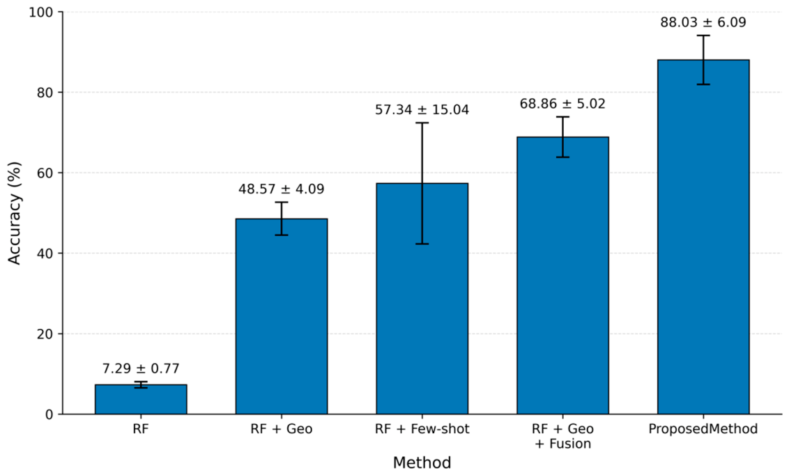
The direct RF model gave the lowest accuracy among the five configurations. Using the 21 input features and source-domain data only, RF achieved an accuracy of 7.29% ± 0.77%, with Macro-F1, balanced accuracy, and MCC of 0.12 ± 0.01, 0.10 ± 0.01, and 0.05 ± 0.01, respectively (Table 3). The F1-scores for mudstone, rhyolite, and fine sandstone were 0.07 ± 0.01, 0.30 ± 0.04, and 0.00 ± 0.00, respectively (Table 4). This low accuracy shows that the source-domain RF model performed poorly when directly applied to the target well, as shown in Figure 11.
Table 3.
Performance of different ablation configurations on the independent target-domain test set.
Table 4.
Class-wise classification performance of different ablation configurations on the independent target-domain test set.
After adding the geoscience-derived features, the accuracy of RF + Geo increased to 48.57% ± 4.09%. The Macro-F1, balanced accuracy, and MCC were 0.46 ± 0.03, 0.45 ± 0.02, and 0.34 ± 0.02, respectively. The F1-scores for mudstone and rhyolite increased to 0.60 ± 0.05 and 0.77 ± 0.03, while fine sandstone remained difficult to classify, with an F1-score of 0.03 ± 0.09 (Table 4). Compared with the direct RF model, the accuracy increased by 41.28 percentage points. The result shows that the additional geoscience-derived features improved the separation of the target-domain lithologies.
The RF + Few-shot model further increased the accuracy to 57.34% ± 15.04%. Its Macro-F1, balanced accuracy, and MCC were 0.71 ± 0.08, 0.77 ± 0.07, and 0.48 ± 0.07, respectively. The F1-scores for mudstone, rhyolite, and fine sandstone were 0.61 ± 0.22, 0.90 ± 0.03, and 0.60 ± 0.12, respectively. Compared with the direct RF model, the few-shot target-domain samples improved the classification of the three target lithologies, particularly rhyolite and fine sandstone. However, the accuracy standard deviation increased to 15.04%, compared with 0.77% for RF and 4.09% for RF + Geo. This indicates that the results were more sensitive to the selection of the few-shot samples.
With geological information and probability fusion, the RF + Geo + Fusion model achieved an accuracy of 68.86% ± 5.02%. The Macro-F1, balanced accuracy, and MCC were 0.64 ± 0.04, 0.69 ± 0.05, and 0.47 ± 0.05, respectively. The F1-scores were 0.77 ± 0.05 for mudstone, 0.72 ± 0.04 for rhyolite, and 0.45 ± 0.14 for fine sandstone. Although its Macro-F1 was lower than that of RF + Few-shot, the accuracy increased by 11.52 percentage points and the standard deviation decreased from 15.04% to 5.02%. This result suggests that the geological constraints helped reduce the variation caused by the limited target-domain samples.
The complete Proposed Method achieved the highest accuracy of 88.03% ± 6.09%. The Macro-F1, balanced accuracy, and MCC were 0.79 ± 0.08, 0.86 ± 0.08, and 0.73 ± 0.11, respectively (Table 3). The F1-scores for mudstone, rhyolite, and fine sandstone were 0.92 ± 0.04, 0.81 ± 0.11, and 0.64 ± 0.18, respectively (Table 4). Compared with the direct RF model, the accuracy increased by 80.74 percentage points. Balanced accuracy increased from 0.10 to 0.86, and MCC increased from 0.05 to 0.73.
Overall, the ablation results show a stepwise improvement from the source-only RF model to the complete framework. The geoscience-derived features improved the feature representation, while the few-shot samples provided target-well information. The addition of geological constraints and probability fusion further improved the prediction and reduced the variation observed in the few-shot model. The complete framework achieved the best overall performance on the independent target-domain test set.
Figure 11.
Ablation study of the proposed method based on classification accuracy.
4.3. Sensitivity Analysis of Key Parameters
It should be emphasized that the sensitivity analyses reported in this section were conducted for robustness verification rather than for parameter selection. The values of the few-shot sample weight ( = 5.0) and the fusion parameters ( = 0.2, = 0.6) were fixed a priori in the methodology (Section 3.6 and Section 3.8), based on established practice and a conservative design principle, before any evaluation was performed. The independent target-domain test set was therefore never used to choose or tune these parameters; it was not used for parameter selection, model fitting, or preprocessing fitting. The sensitivity analyses were conducted post hoc for robustness assessment only, and were used only for final performance reporting.
4.3.1. Sensitivity Analysis of Few-Shot Sample Weight
The effect of the few-shot sample weight was examined while keeping the regular training sample weight . The few-shot target-domain sample weight was set to . For each setting, the complete transfer-learning procedure was repeated with 10 random seeds. Figure 12 shows the mean accuracy and standard deviation obtained for each weight.
Figure 12.
Sensitivity analysis of the few-shot target-domain sample weight
The mean accuracy changed only slightly when varied from 1 to 7. The corresponding accuracies were 88.69%, 88.52%, 88.69%, 88.03%, and 88.20% for = 1, 2, 3, 5 and 7, respectively. At , the accuracy decreased to 86.89%. The difference between the highest and lowest mean accuracy over all tested values was 1.80 percentage points. Thus, the model was not strongly affected by the exact weight assigned to the few-shot samples within the range of 1–7.
The error bars in Figure 12 show the variation among the 10 random-seed runs. In particular, the large variation observed in the few-shot experiments is mainly related to the limited number of target-domain samples available for adaptation. Increasing does not produce a continuous increase in accuracy. When the weight reaches 10, the performance instead decreases, suggesting that excessive emphasis on the small target-domain sample set may weaken the contribution of the source-domain data.
These results confirm that the value = 5.0, fixed a priori in Section 3.6, lies within the stable region (1–7), where the accuracy varies by only 1.80 percentage points. The model was therefore insensitive to the exact weight, and the a priori choice of = 5.0 was retained for the final model without any adjustment based on test-set performance. This moderate weight gives sufficient emphasis to the target-domain samples without assigning excessive weight to the limited few-shot data.
4.3.2. Sensitivity Analysis of Adaptive Fusion Parameters
The adaptive fusion parameters control the range of geological-constraint contribution in the final lithology probability. Their effects were evaluated separately by varying and . For each parameter setting, the complete few-shot transfer-learning procedure was repeated with 10 random seeds. The mean accuracy and standard deviation are shown in Figure 13.
Figure 13.
Sensitivity analysis of the adaptive fusion parameters.
Sensitivity to . With = 0.2 fixed, was varied from 0.4 to 0.8. As shown in Figure 13a, the mean accuracy increased from 82.79% at = 0.4 to 89.51% at = 0.8. The intermediate values of 0.5, 0.6, and 0.7 gave accuracies of 86.39%, 88.03%, and 89.02%, respectively. The standard deviation also decreased as increased, from 15.98% at 0.4 to 5.25% at 0.8. Thus, within the tested range, a larger upper bound allowed a greater contribution from the geological constraint and was associated with both higher mean accuracy and lower variation among the 10 runs.
Sensitivity to . With = 0.6 fixed, was varied from 0.0 to 0.4. The mean accuracy increased gradually from 87.05% to 89.02% as increased from 0.0 to 0.4. The accuracies at = 0.1, 0.2, and 0.3 were 87.54%, 88.03%, and 88.52%, respectively (Figure 13b). The standard deviations remained relatively large over the tested range, and no clear monotonic change was observed. The increase in mean accuracy suggests that allowing the geological constraint to retain a minimum contribution is beneficial for the target-domain prediction under the present experimental conditions.
The two sensitivity tests show that the fusion parameters have a measurable effect on the classification results. Increasing had a more pronounced effect than increasing , particularly in terms of accuracy variation. However, the highest accuracy was obtained at the upper end of the tested parameter ranges rather than at the final settings used in the proposed model.
Therefore, = 0.2 and = 0.6 were retained for the final model, consistent with the values fixed a priori in Section 3.8. Notably, these parameters were not selected to maximize test-set accuracy; The higher accuracy observed at the upper end of the tested range ( = 0.8) is reported only as a post-hoc sensitivity result and was not used to modify the predefined parameters. This setting avoids assigning an excessive contribution to the geological prior while maintaining a nonzero lower bound for its contribution to the final prediction.
4.4. Comparison of Geological Constraint Strategies
Three geological constraint strategies were compared under the same few-shot cross-well lithology recognition framework: hard threshold, probabilistic soft constraint, and uncertainty-aware fusion. The source and target data, few-shot samples, SMOTE, quantile transformation, and RF classifier were kept unchanged. The three methods differed only in how geological constraints were represented and combined with the RF prediction. Each method was tested with 10 random seeds. The results are listed in Table 5 and shown in Figure 14.
Table 5.
Performance comparison of different geological constraint strategies.
Figure 14.
Comparison of classification accuracy for different geological constraint strategies.
The hard-threshold method achieved an accuracy of 81.15% ± 18.21%, with a Macro-F1 of 0.78 ± 0.09, balanced accuracy of 0.85 ± 0.09, and MCC of 0.67 ± 0.14. The probabilistic soft-constraint method increased the accuracy to 84.43% ± 13.46%, with Macro-F1, balanced accuracy, and MCC of 0.79 ± 0.09, 0.86 ± 0.09, and 0.70 ± 0.14, respectively. Compared with the hard-threshold method, the accuracy increased by 3.28 percentage points and the standard deviation decreased by 4.75 percentage points.
The uncertainty-aware fusion method achieved the highest accuracy of 88.03% ± 6.09%. Its Macro-F1, balanced accuracy, and MCC were 0.79 ± 0.08, 0.86 ± 0.08, and 0.73 ± 0.11, respectively. Compared with the probabilistic soft-constraint method, the accuracy increased by 3.60 percentage points, while the standard deviation decreased by 7.37 percentage points. MCC also increased from 0.70 to 0.73, whereas Macro-F1 and balanced accuracy remained similar.
The results show that the three strategies provide different levels of geological constraint. The probabilistic soft constraint performed better than the binary threshold method, while the uncertainty-aware fusion further improved accuracy and reduced the variation among the 10 runs. Among the three strategies, the uncertainty-aware fusion method gave the highest accuracy and MCC and the lowest standard deviation.
4.5. Comparison with Representative Transfer Learning and Few-Shot Methods
To further evaluate the proposed method, four representative transfer learning and few-shot learning methods were selected for comparison: CORAL, a shared-class CORAL variant, similarity-weighted transfer, and a prototype-based few-shot classifier. CORAL was used as a representative statistical domain adaptation method, while similarity-weighted transfer represents instance-level transfer learning. The prototype-based classifier represents few-shot learning based on class prototypes. The shared-class CORAL variant was included to examine the effect of the label-space mismatch between the source and target domains.
All methods were evaluated using the same cross-well setting. XX-1, XX-2, and XX-3 were used as the source domain, and an independent fourth well was used as the target domain. Three labeled samples from each target-domain lithology class were used for few-shot adaptation, and the remaining target samples were reserved for independent testing. The same SMOTE and quantile transformation procedures were used where applicable, and RF was used for the RF-based methods. Each experiment was repeated with 10 random seeds. The results are summarized in Table 6 and Figure 15.
Table 6.
Quantitative comparison of representative transfer learning and few-shot learning methods for cross-well lithology recognition.
Figure 15.
Accuracy comparison of representative transfer learning and few-shot learning methods.
For the baselines, the following hyperparameter settings were used. CORAL [20] is a closed-form second-order covariance alignment that has no tunable hyperparameters; source features were aligned to the target domain using the mean and covariance of all target-well features (transductive domain adaptation, using only unlabeled features and never the labels). The shared-class CORAL variant aligned only the source samples whose labels overlap with the target domain. The similarity-weighted transfer method used a Gaussian-kernel instance weight, whose bandwidth was determined automatically as the median distance from the source samples to the target-domain centroid, so it required no manual tuning. The prototype-based few-shot classifier has no tunable hyperparameters. All RF-based baselines used exactly the same random-forest hyperparameters as the proposed method (400 decision trees, a maximum tree depth of 40, and log2-based feature selection at each split). All baselines thereby followed the same few-shot, SMOTE, quantile-transformation, and independent-testing protocol described above.
The CORAL + RF method achieved an accuracy of 26.56% ± 6.13%, with a Macro-F1 of 0.49 ± 0.06, balanced accuracy of 0.52 ± 0.07, and MCC of 0.25 ± 0.05. The shared-class CORAL + RF method increased the accuracy to 38.36% ± 6.73% and the balanced accuracy to 0.72 ± 0.06. However, the Macro-F1 was 0.40 ± 0.07 and MCC was 0.31 ± 0.04. Restricting the source data to the lithologies shared with the target well improved the balanced accuracy, but the overall classification performance remained limited. Under the present experimental setting, covariance alignment alone provided limited performance.
The similarity-weighted transfer method performed better, with an accuracy of 69.18% ± 16.47%, Macro-F1 of 0.76 ± 0.09, balanced accuracy of 0.80 ± 0.10, and MCC of 0.55 ± 0.11. The prototype-based few-shot classifier achieved 76.72% ± 11.14% accuracy, with a Macro-F1 of 0.69 ± 0.06, balanced accuracy of 0.86 ± 0.04, and MCC of 0.62 ± 0.08. Both methods made better use of target-domain information than CORAL. However, their accuracy variations were relatively large, with standard deviations of 16.47% and 11.14%, respectively.
The proposed method achieved the highest accuracy of 88.03% ± 6.09%. Its Macro-F1, balanced accuracy, and MCC were 0.79 ± 0.08, 0.86 ± 0.08, and 0.73 ± 0.11, respectively. Compared with the similarity-weighted transfer and prototype-based few-shot classifier, the accuracy increased by 18.85 and 11.31 percentage points, respectively. The proposed method also had the lowest accuracy standard deviation among the five methods. Its standard deviation was 6.09%, compared with 16.47% for similarity-weighted transfer and 11.14% for the prototype-based classifier. A paired Wilcoxon signed-rank test over the 10 shared random seeds further confirmed that the proposed method’s accuracy was significantly higher than that of CORAL + RF, the shared-class CORAL + RF, and similarity-weighted transfer + RF, and marginally higher than that of the prototype-based few-shot classifier (Table 7).
Table 7.
Paired Wilcoxon signed-rank test p-values of the proposed method versus each comparison method across the 10 shared random seeds.
The comparison shows that the methods based only on statistical alignment or target-domain samples have limited performance when the source and target wells differ in both lithology composition and feature distributions. The proposed method uses the few-shot target samples together with geological constraints and uncertainty-aware fusion. Under the same test conditions, this combination gave higher accuracy and MCC, with less variation between different random seeds. To further quantify the sampling uncertainty, 95% confidence intervals for the proposed method are reported in Table 8, distinguishing the variation across random seeds from the test-set sampling noise. As shown, the bootstrap interval provides an estimate of the sampling uncertainty associated with the held-out target-domain test set and complements the seed-level uncertainty analysis.
Table 8.
The 95% confidence interval of the mean performance across random seeds.
4.6. Limitations and Future Work
The main limitation of this study is the limited number of wells and labeled lithological samples. The available data cover only a limited range of geological conditions and logging responses. As a result, the proposed method could not be evaluated using a larger number of source–target well combinations. Its performance in other wells and geological settings therefore needs further testing.
This issue is particularly important for volcanic reservoirs, where lithology, mineral composition, pore structure, and logging responses can vary between wells. Although few-shot target-domain samples and geoscience constraints were used to account for part of these differences, more data are needed for a broader evaluation. The results of this study should therefore be considered within the current dataset and experimental conditions.
A leave-one-well-out evaluation, in which each available well is treated in turn as the target domain, is not directly applicable to the present dataset because the four wells have almost non-overlapping lithology compositions. Specifically, XX-2 contains only dacite; XX-3 contains dacite, diorite, and tuff; XX-1 contains granite, rhyolite, mudstone, tuff, and fine sandstone; and the target well contains only mudstone, rhyolite, and fine sandstone. Under most single-well target scenarios, the source domain would therefore lack one or more of the target-well classes (e.g., granite and diorite each occur in only one well), and these classes could not be learned by any model. A fair leave-one-well-out comparison is thus infeasible with the currently available wells; additional wells with overlapping lithology classes are required to support such validation, which is an important direction for future work.
Future work will focus on adding more wells and labeled samples. This will allow more source–target combinations to be tested and provide additional data for evaluating the generalization of the proposed method. The larger dataset can also be used to further examine the few-shot adaptation and geoscience constraints under different cross-well conditions.
5. Conclusions
This study developed a geoscience knowledge-guided machine-learning method for cross-well lithology recognition in heterogeneous volcanic reservoirs. The main conclusions are as follows:
- (1)
- Geochemical features and elemental ratios complement conventional logging data and provide additional information for lithology discrimination across wells.
- (2)
- Few-shot target-well samples, together with feature alignment and sample weighting, improve model adaptation under limited labeled-data conditions.
- (3)
- Probabilistic geological constraints and uncertainty-aware fusion improve the consistency of model predictions with geological knowledge while avoiding rigid classification rules.
- (4)
- With three source wells and one independent target well, and only three labeled samples per lithology class for adaptation, the proposed method achieved an accuracy of 88.03 ± 6.09% across 10 random seeds, with Macro-F1, balanced accuracy, and MCC of 0.79 ± 0.08, 0.86 ± 0.08, and 0.73 ± 0.11, respectively. The results support the use of geoscience knowledge and few-shot learning for cross-well lithology recognition, although further validation on larger and more diverse datasets is needed.
Author Contributions
Methodology, Q.Z. and J.W.; Formal analysis, S.W.; Investigation, S.W.; Data curation, Y.G.; Writing—review & editing, Y.G. and J.W. All authors have read and agreed to the published version of the manuscript.
Funding
This research received no external funding.
Data Availability Statement
The data presented in this study are available on request from the corresponding author due to restrictions related to data confidentiality and ownership.
Conflicts of Interest
Authors Qibin Zhao and Shiyue Wang were employed by China Offshore Petroleum (China) Co., Ltd.; Authors Yongde Gao and Jinbo Wu were employed by CNOOC China Limited Zhanjiang Branch. The authors declare that the research was conducted in the absence of any commercial or financial relationships that could be construed as a potential conflict of interest.
References
- Serra, O. Fundamentals of Well-Log Interpretation, Part 1: The Acquisition of Logging Data; Elsevier: Amsterdam, The Netherlands, 1984. [Google Scholar]
- Ellis, D.V.; Singer, J.M. Well Logging for Earth Scientists, 2nd ed.; Springer: Dordrecht, The Netherlands, 2007. [Google Scholar]
- Xie, Y.; Zhu, C.; Zhou, W.; Li, Z.; Liu, X.; Tu, M. Evaluation of machine learning methods for formation lithology identification: A comparison of tuning processes and model performances. J. Pet. Sci. Eng. 2018, 160, 182–193. [Google Scholar] [CrossRef] [Scilit]
- Liu, H.; Wu, Y.; Cao, Y.; Lv, W.; Han, H.; Li, Z.; Chang, J. Well Logging Based Lithology Identification Model Establishment Under Data Drift: A Transfer Learning Method. Sensors 2020, 20, 3643. [Google Scholar] [CrossRef] [Scilit] [PubMed]
- Dong, S.-Q.; Zhong, Z.-H.; Cui, X.-H.; Zeng, L.-B.; Yang, X.; Liu, J.-J.; Sun, Y.-M.; Hao, J.-R. A deep kernel method for lithofacies identification using conventional well logs. Pet. Sci. 2023, 20, 1411–1428. [Google Scholar] [CrossRef] [Scilit]
- Breiman, L. Random forests. Mach. Learn. 2001, 45, 5–32. [Google Scholar] [CrossRef] [Scilit]
- Cortes, C.; Vapnik, V. Support-vector networks. Mach. Learn. 1995, 20, 273–297. [Google Scholar] [CrossRef] [Scilit]
- Friedman, J.H. Greedy function approximation: A gradient boosting machine. Ann. Stat. 2001, 29, 1189–1232. [Google Scholar] [CrossRef] [Scilit]
- Li, Z.; Li, P.; Liu, Z.; Cui, Y. Single-well lithofacies identification based on logging response and convolutional neural network. J. Appl. Geophys. 2022, 207, 104865. [Google Scholar] [CrossRef] [Scilit]
- Pan, S.J.; Yang, Q. A survey on transfer learning. IEEE Trans. Knowl. Data Eng. 2010, 22, 1345–1359. [Google Scholar] [CrossRef] [Scilit]
- Zhuang, F.; Qi, Z.; Duan, K.; Xi, D.; Zhu, Y.; Zhu, H.; Xiong, H.; He, Q. A comprehensive survey on transfer learning. Proc. IEEE 2021, 109, 43–76. [Google Scholar] [CrossRef] [Scilit]
- Long, M.; Cao, Y.; Wang, J.; Jordan, M. Learning transferable features with deep adaptation networks. In Proceedings of the 32nd International Conference on Machine Learning (ICML 2015), Lille, France, 7–9 July 2015; pp. 97–105. [Google Scholar]
- Weiss, K.; Khoshgoftaar, T.M.; Wang, D. A survey of transfer learning. J. Big Data 2016, 3, 9. [Google Scholar] [CrossRef] [Scilit]
- Ganin, Y.; Ustinova, E.; Ajakan, H.; Germain, P.; Larochelle, H.; Laviolette, F.; Marchand, M.; Lempitsky, V. Domain-adversarial training of neural networks. J. Mach. Learn. Res. 2016, 17, 1–35. [Google Scholar]
- Reichstein, M.; Camps-Valls, G.; Stevens, B.; Jung, M.; Denzler, J.; Carvalhais, N.; Prabhat, F. Deep learning and process understanding for data-driven Earth system science. Nature 2019, 566, 195–204. [Google Scholar] [CrossRef] [Scilit] [PubMed]
- Karpatne, A.; Atluri, G.; Faghmous, J.H.; Steinbach, M.; Banerjee, A.; Ganguly, A.; Shekhar, S.; Samatova, N.; Kumar, V. Theory-guided data science: A new paradigm for scientific discovery from data. IEEE Trans. Knowl. Data Eng. 2017, 29, 2318–2331. [Google Scholar] [CrossRef] [Scilit]
- Zhang, B.; Wang, P.; Zhang, G.; Sun, X.; Lu, B.; Ni, W. Cenozoic volcanic rocks in the Pearl River Mouth and Southeast Hainan Basins of South China Sea and their implications for petroleum geology. Pet. Explor. Dev. 2013, 40, 704–713. [Google Scholar] [CrossRef] [Scilit]
- Zou, C.; Zhao, W.; Jia, C.; Zhu, R.; Zhang, G.; Zhao, X.; Yuan, X. Formation and distribution of volcanic hydrocarbon reservoirs in sedimentary basins of China. Pet. Explor. Dev. 2008, 35, 257–271. [Google Scholar] [CrossRef] [Scilit]
- Pan, S.J.; Tsang, I.W.; Kwok, J.T.; Yang, Q. Domain adaptation via transfer component analysis. IEEE Trans. Neural Netw. 2011, 22, 199–210. [Google Scholar] [CrossRef] [Scilit] [PubMed]
- Sun, B.; Feng, J.; Saenko, K. Return of frustratingly easy domain adaptation. Proc. AAAI Conf. Artif. Intell. 2016, 30, 2058–2065. [Google Scholar] [CrossRef] [Scilit]
- Sun, L.; Li, Z.; Li, K.; Liu, H.; Liu, G.; Lv, W. Cross-well lithology identification based on wavelet transform and adversarial learning. Energies 2023, 16, 1475. [Google Scholar] [CrossRef] [Scilit]
- Xu, B.; Feng, Z.; Zhou, J.; Shao, R.; Wu, H.; Liu, P.; Tian, H.; Li, W.; Xiao, L. Transfer learning for well logging formation evaluation using similarity weights. Artif. Intell. Geosci. 2024, 5, 100091. [Google Scholar] [CrossRef] [Scilit]
- Li, J.; Wang, J.; Li, Z.; Kang, Y.; Lv, W. Partial domain adaptation for building borehole lithology model under weaker geological prior. IEEE Trans. Artif. Intell. 2024, 5, 6645–6658. [Google Scholar] [CrossRef] [Scilit]
- Snell, J.; Swersky, K.; Zemel, R. Prototypical networks for few-shot learning. Adv. Neural Inf. Process. Syst. 2017, 30, 4077–4087. [Google Scholar]
- Sun, Y.; Pang, S.; Zhao, Z.; Zhang, Y. Interpretable SHAP model combining meta-learning and vision transformer for lithology classification using limited and unbalanced drilling data. Nat. Resour. Res. 2024, 33, 2545–2565. [Google Scholar] [CrossRef] [Scilit]
- Sun, Y.; Pang, S.; Qiu, Z.; Zhang, Y. Efficient lithology classification from small-sample well logging data processed by wavelet thresholding algorithm: Integrating meta-learning with self-attention mechanism model. Geoenergy Sci. Eng. 2024, 246, 213629. [Google Scholar] [CrossRef] [Scilit]
- Wang, A.; Zhao, S.; Xie, K.; Wen, C.; Tian, H.-L.; He, J.-B.; Zhang, W. Attention mechanism-enhanced graph convolutional neural network for unbalanced lithology identification. Sci. Rep. 2024, 14, 17319. [Google Scholar] [CrossRef] [Scilit] [PubMed]
- Li, H.; Sun, Y.; Qiao, S. Enhanced lithology identification with few-shot well-logging data using a confidence-enhanced semi-supervised meta-learning approach. Measurement 2025, 247, 116762. [Google Scholar] [CrossRef] [Scilit]
- Chen, B.; Zeng, X.; Cao, S.; Zhang, W.; Xu, S.; Zhang, B.; Hou, Z. Interwell stratigraphic correlation detection based on knowledge-enhanced few-shot learning. J. Pet. Sci. Eng. 2022, 219, 111187. [Google Scholar] [CrossRef] [Scilit]
- Zhao, Z.; Zhou, D.; Liao, J. Tertiary paleogeography and depositional evolution in the Pearl River Mouth Basin of the northern South China Sea. J. Trop. Oceanogr. 2009, 28, 52–60. [Google Scholar] [CrossRef]
- Zhao, F.; Wu, S.; Sun, Q.; Huuse, M.; Li, W.; Wang, Z. Submarine volcanic mounds in the Pearl River Mouth Basin, northern South China Sea. Mar. Geol. 2014, 355, 162–172. [Google Scholar] [CrossRef] [Scilit]
- Wu, J.; Zhang, G.; Wang, P.; Xie, X.; Hu, S.; Qi, J. Geological Response and Forming Mechanisms of 23.8 Ma Tectonic Events in Deepwater Area of the Pearl River Mouth Basin in South China Sea. Earth Sci. 2012, 37, 654–666. [Google Scholar] [CrossRef]
- Li, M.; Fan, C.W.; Liu, K.; Chen, L. Genesis and distribution prediction of fractures in buried igneous rocks around the Qionghai Uplift, western Pearl River Mouth Basin. Mar. Geol. Quat. Geol. 2026, 1–11. [Google Scholar] [CrossRef]
- Carvalho, H.M.O.; Daniel, H.; Korenchendler, A.; Sobreira, M.C.A.; Machado, A.M.C. Lithology classification based on well log data: A benchmark for machine learning models. Math. Geosci. 2026. [Google Scholar] [CrossRef] [Scilit]
- Zhang, J.; He, Y.; Zhang, Y.; Li, W.; Zhang, J. Well-logging-based lithology classification using machine learning methods for high-quality reservoir identification: A case study of Baikouquan Formation in Mahu Area of Junggar Basin, NW China. Energies 2022, 15, 3675. [Google Scholar] [CrossRef] [Scilit]
- Shuvo, M.A.I.; Joy, S.M.H. A data driven approach to assess the petrophysical parametric sensitivity for lithology identification based on ensemble learning. J. Appl. Geophys. 2024, 222, 105330. [Google Scholar] [CrossRef] [Scilit]
- Yoshihara, N.; Nakashima, Y.; Kiho, K.; Ikawa, R. Random forest-based lithology identification using geophysical well logging data along a borehole in a coastal aquifer in Suruga Bay, Japan. Earth Sci. Inform. 2026, 19, 157. [Google Scholar] [CrossRef] [Scilit]
- Bergstra, J.; Bengio, Y. Random search for hyper-parameter optimization. J. Mach. Learn. Res. 2012, 13, 281–305. [Google Scholar]
- Yin, P.; Qi, L.; Zhu, Q.; Luo, L.; Tang, J.; Ruan, C.; Zhao, L.; Liang, H. Application of element logging to lithologic identification of key horizons in Sichuan–Chongqing gas provinces. Nat. Gas. Ind. B 2018, 5, 132–138. [Google Scholar] [CrossRef] [Scilit]
- Klaja, J.; Dudek, L. Geological interpretation of spectral gamma ray (SGR) logging in selected boreholes. Nafta-Gaz 2016, 72, 3–14. [Google Scholar] [CrossRef] [Scilit]
- Wang, L.; Mao, Z.; Sun, Z.; Luo, X.; Song, Y.; Liu, Z. Genesis analysis of high-gamma ray sandstone reservoir and its log evaluation techniques: A case study from the Junggar Basin, Northwest China. Sci. World J. 2013, 2013, 848201. [Google Scholar] [CrossRef] [Scilit] [PubMed]
- Gould, K.M.; Piper, D.J.W.; Pe-Piper, G.; MacRae, R.A. Facies, provenance and paleoclimate interpretation using spectral gamma logs: Application to the Lower Cretaceous of the Scotian Basin. Mar. Pet. Geol. 2014, 57, 445–454. [Google Scholar] [CrossRef] [Scilit]
- Huang, B.; Pan, B. Characteristics of log responses and lithology determination of igneous rock reservoirs. J. Geophys. Eng. 2004, 1, 51–55. [Google Scholar] [CrossRef] [Scilit]
- Bartetzko, A. Gamma ray spectrometric analysis of hydrothermally altered dacite samples from the PACMANUS hydrothermal field: Implications for the interpretation of gamma ray wireline measurements. J. Volcanol. Geotherm. Res. 2008, 175, 269–277. [Google Scholar] [CrossRef] [Scilit]
- Duan, Y.; Xie, J.; Su, Y.; Liang, H.; Hu, X.; Wang, Q.; Pan, Z. Application of the decision tree method to lithology identification of volcanic rocks—Taking the Mesozoic in the Laizhouwan Sag as an example. Sci. Rep. 2020, 10, 19209. [Google Scholar] [CrossRef] [Scilit] [PubMed]
- Li, R.; Xiong, Z.; Wang, Z.; Xie, W.; Li, W.; Su, N. Lithofacies, mineralogy, and pore characteristics of Permian marine tuffaceous rocks in the Sichuan Basin. Front. Earth Sci. 2023, 10, 1054276. [Google Scholar] [CrossRef] [Scilit]
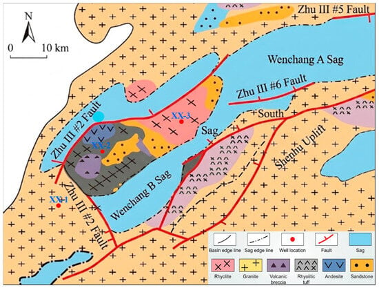
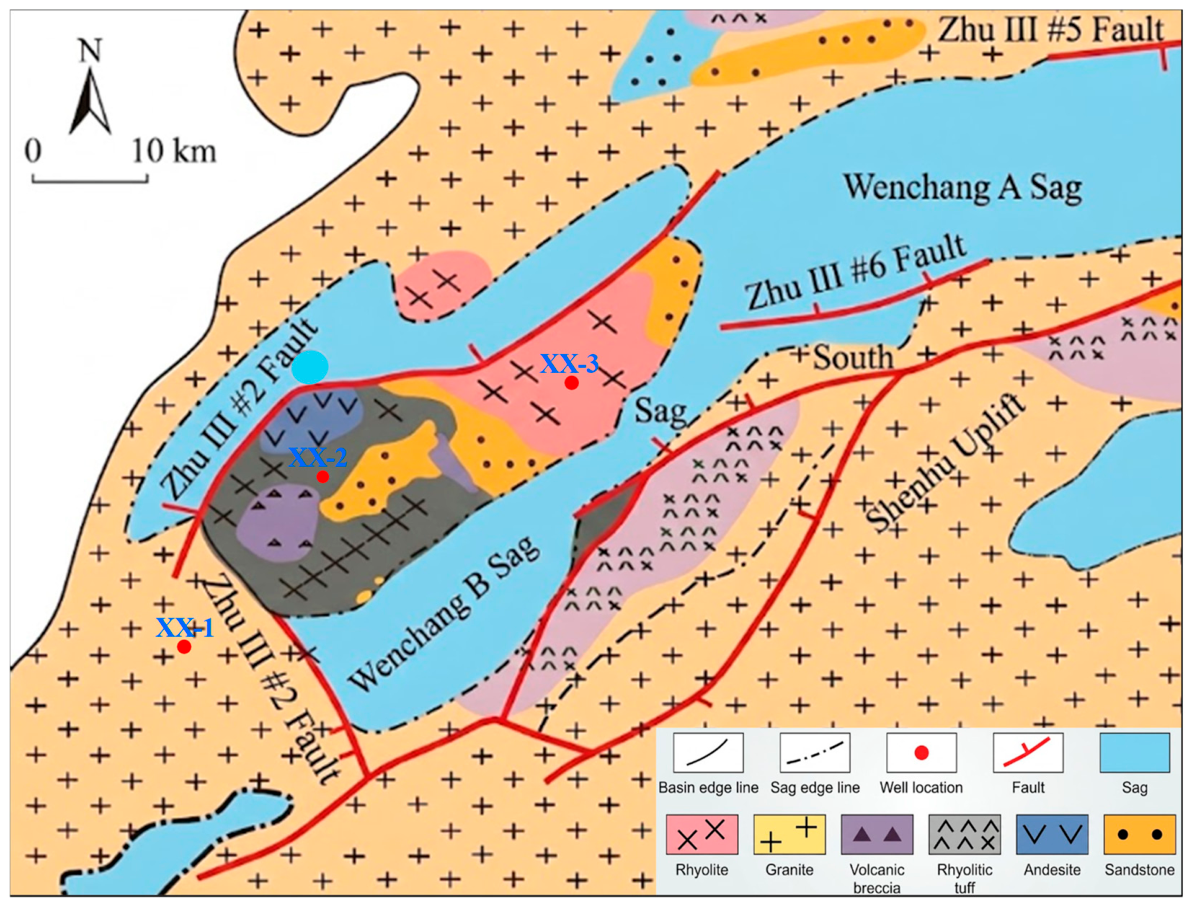
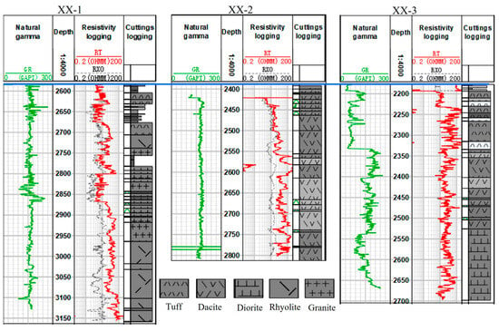
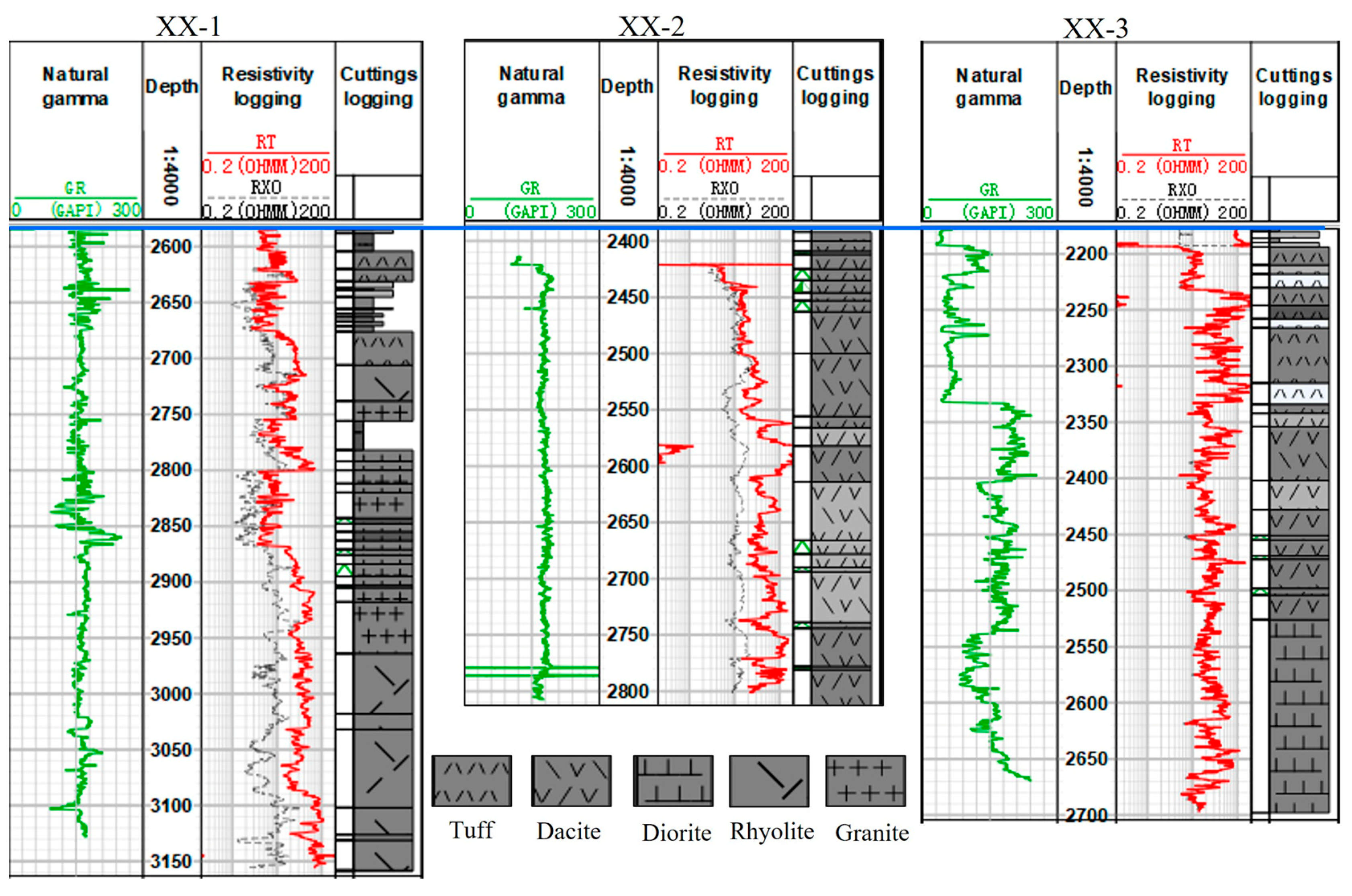
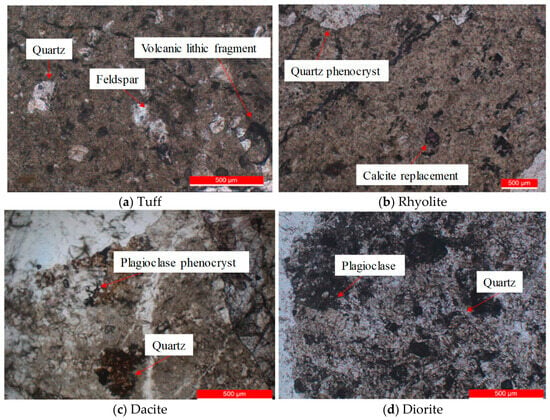
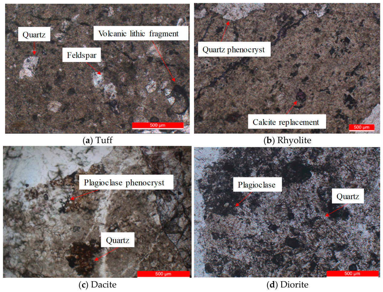
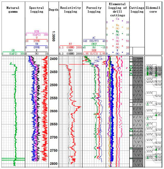
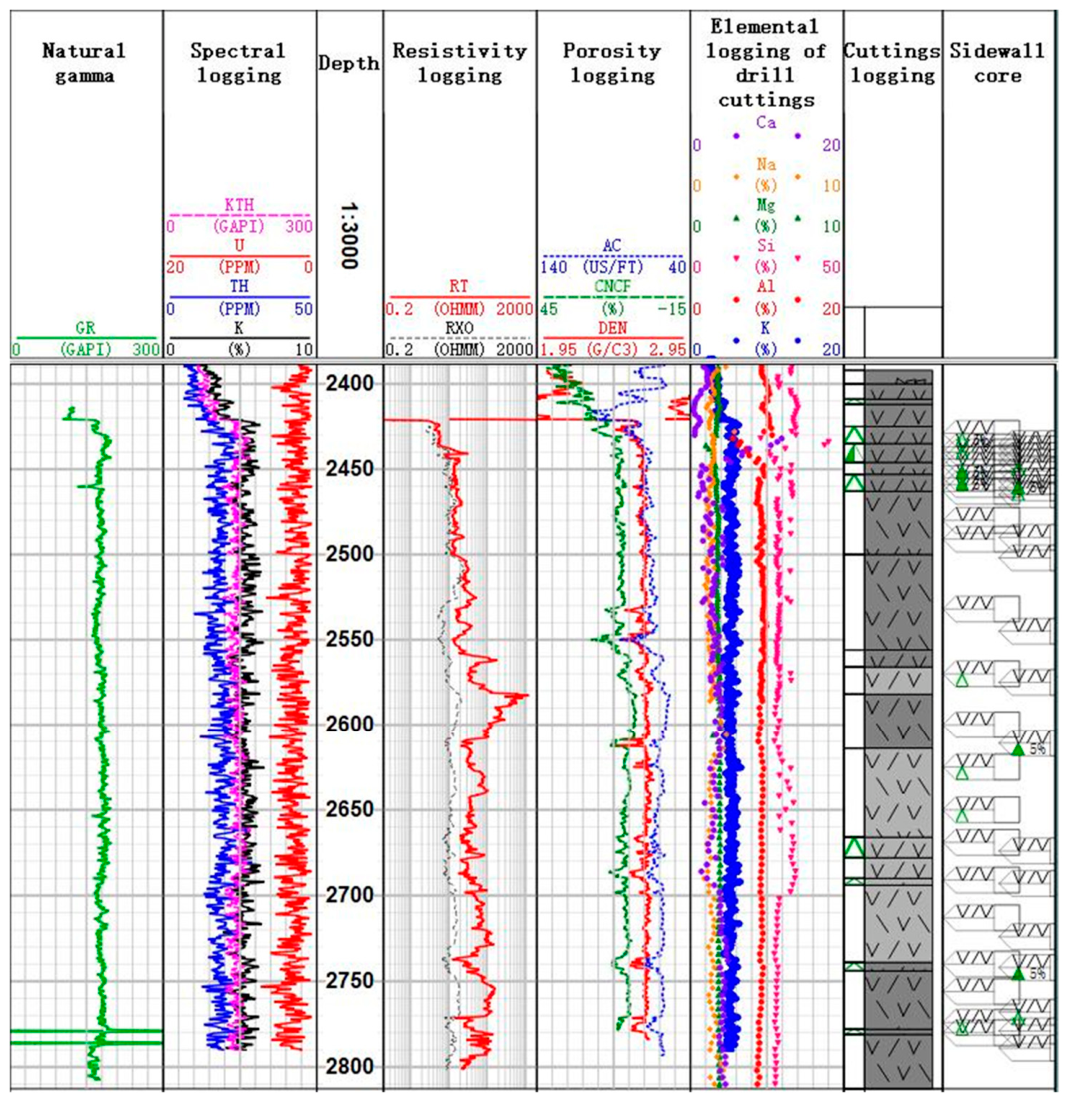
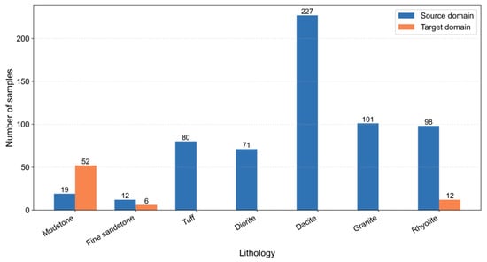
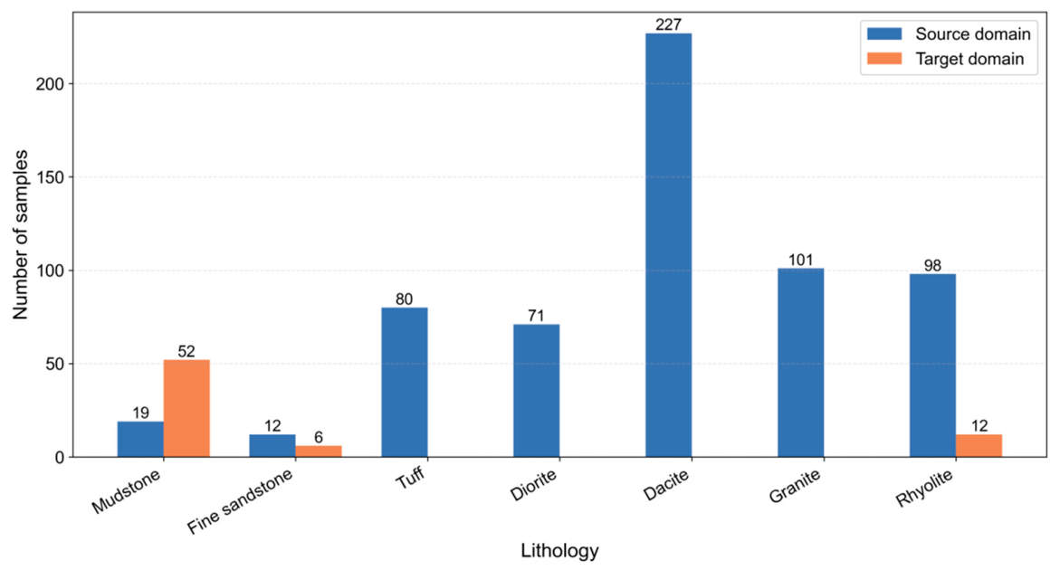
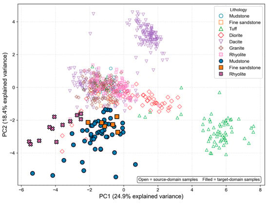
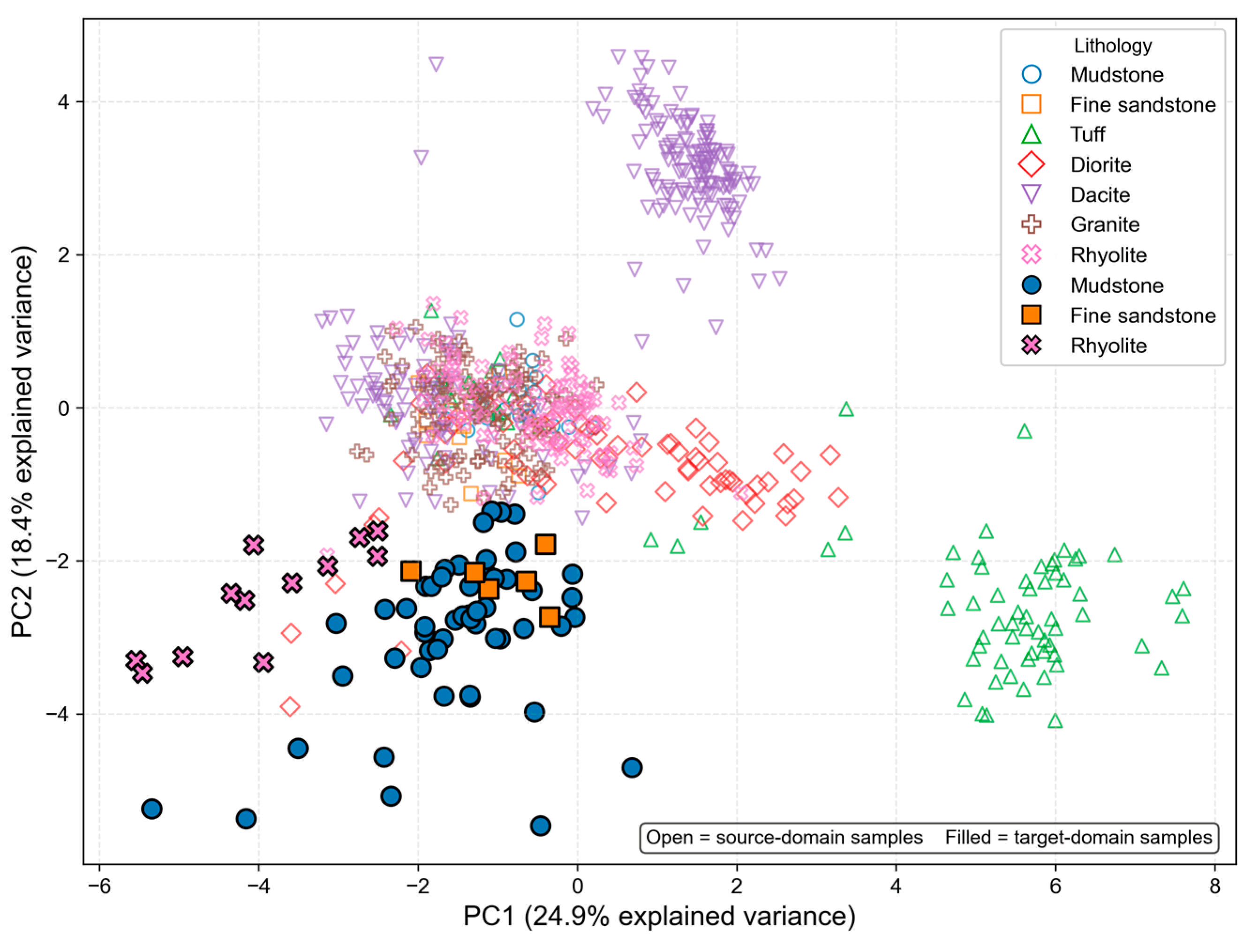
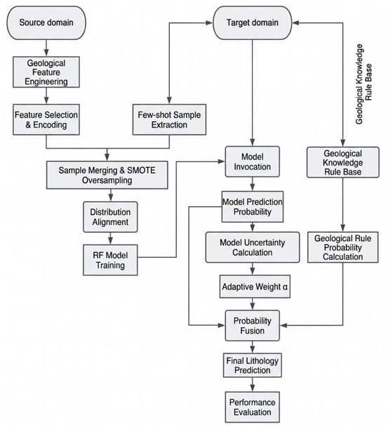
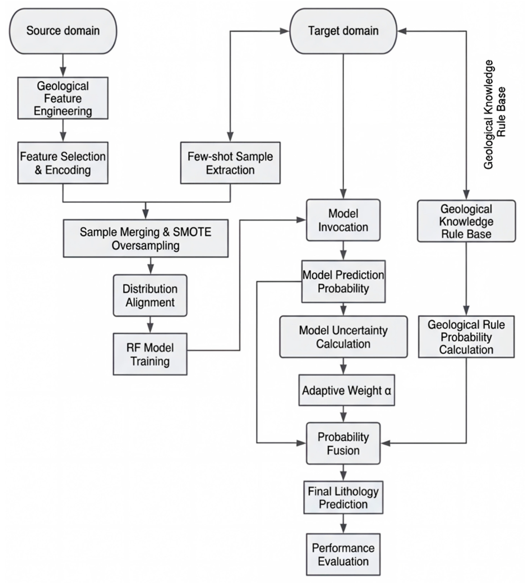
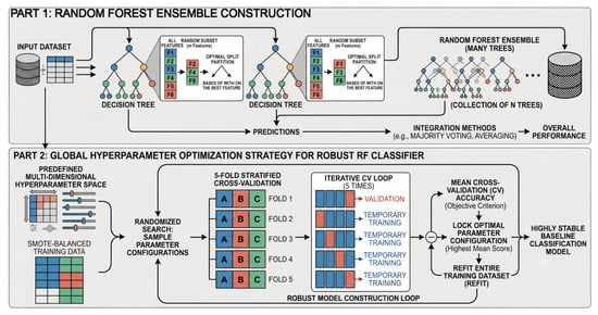
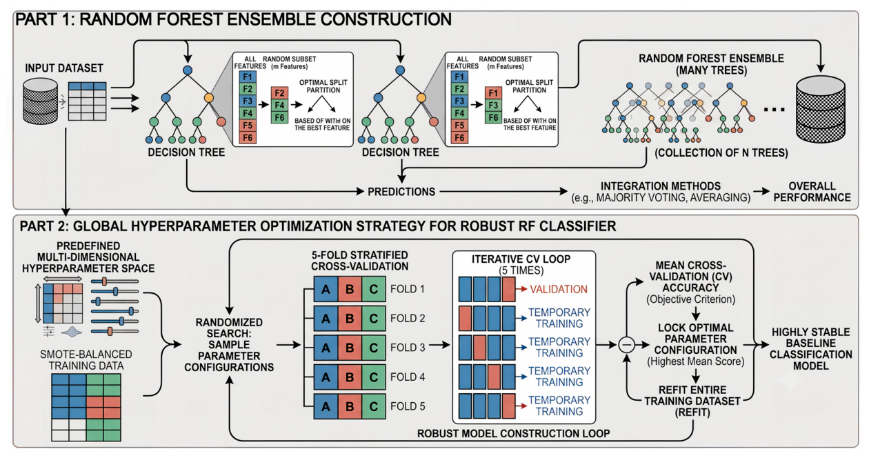
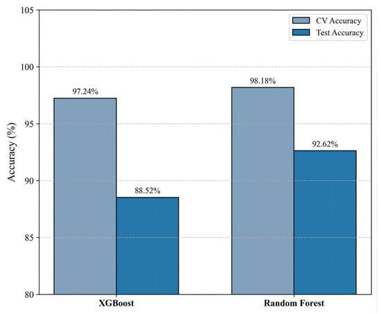
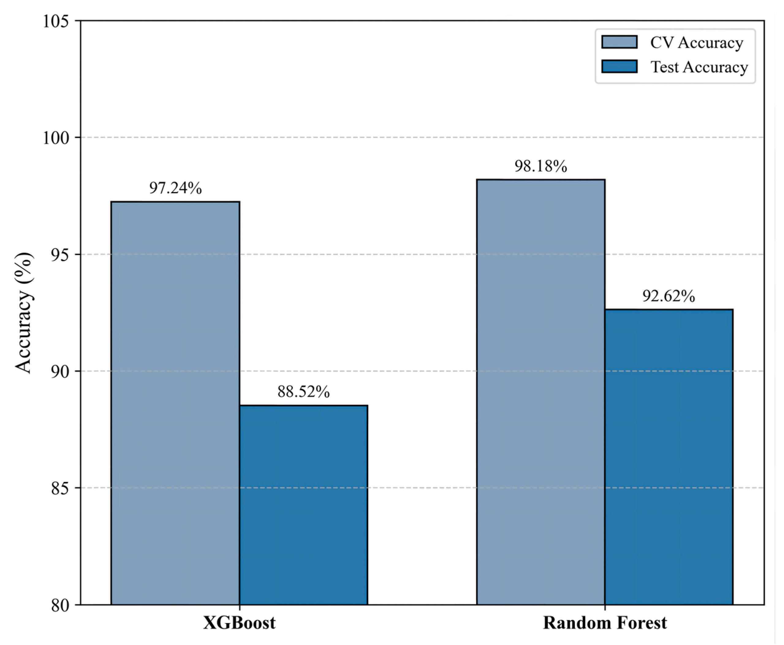
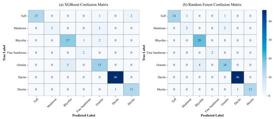
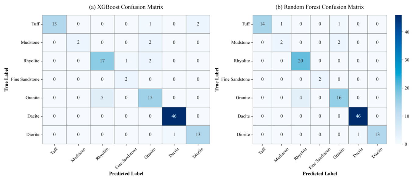
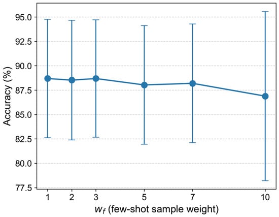
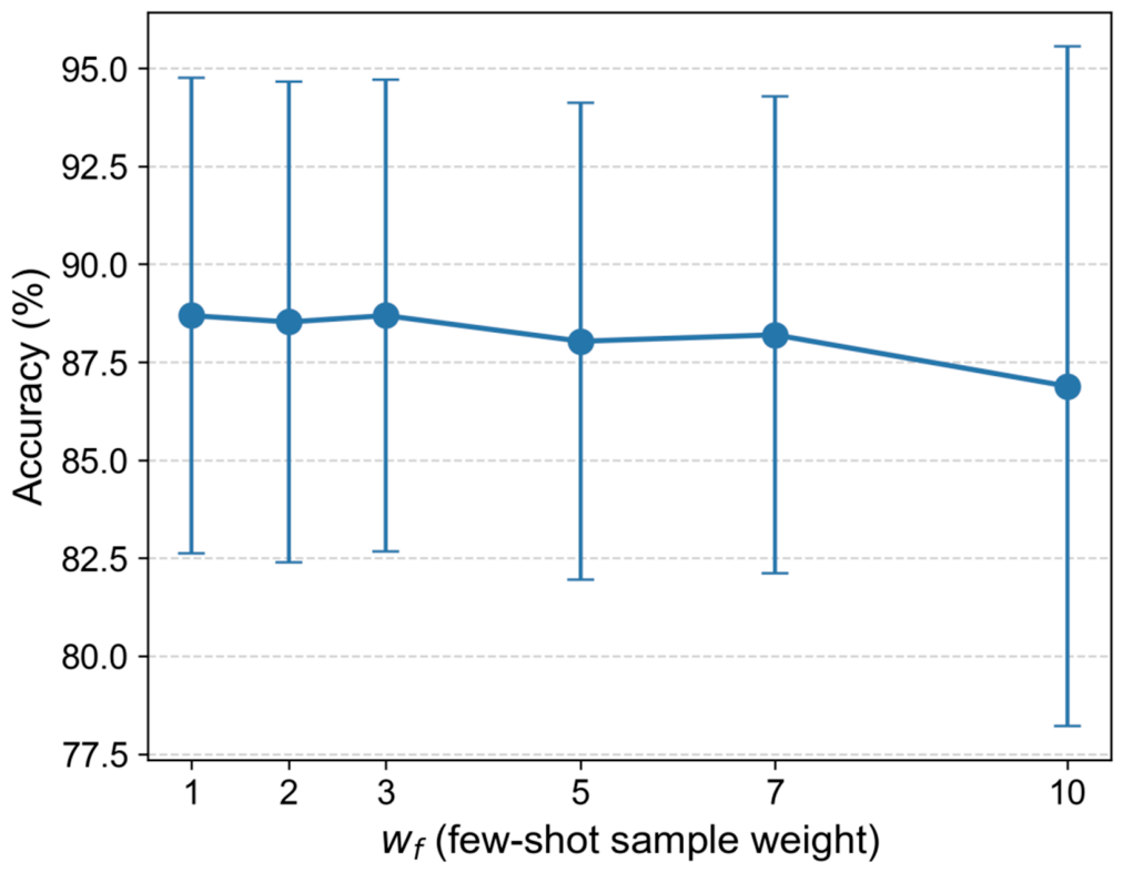
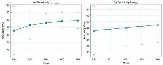
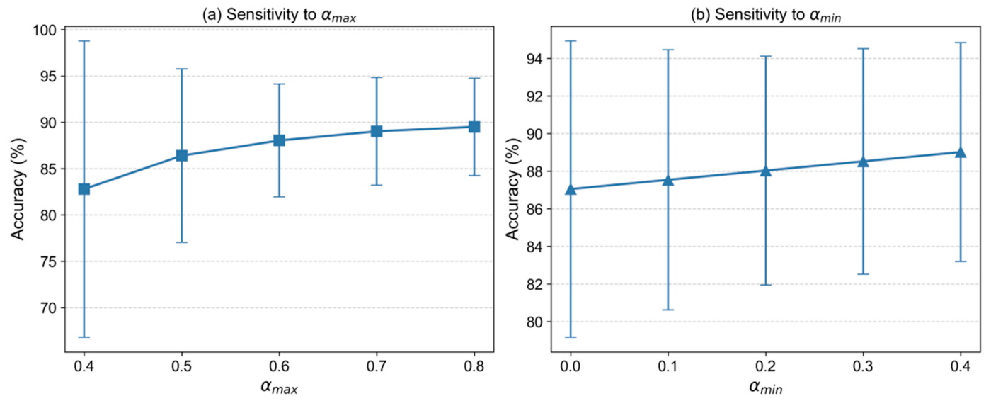
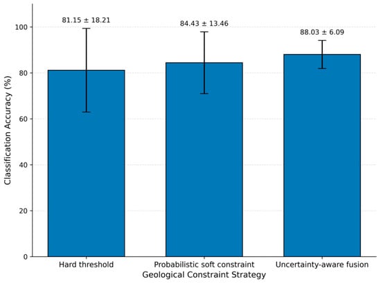
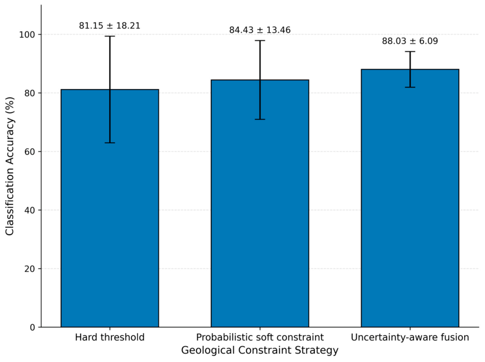
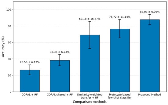
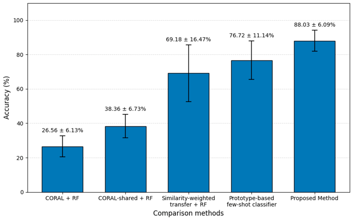

Disclaimer/Publisher’s Note: The statements, opinions and data contained in all publications are solely those of the individual author(s) and contributor(s) and not of MDPI and/or the editor(s). MDPI and/or the editor(s) disclaim responsibility for any injury to people or property resulting from any ideas, methods, instructions or products referred to in the content. |
© 2026 by the authors. Licensee MDPI, Basel, Switzerland. This article is an open access article distributed under the terms and conditions of the Creative Commons Attribution (CC BY) license.