


Abstract
With the rapid development of graph neural networks and physics-informed machine learning for critical infrastructure risk, reliable assessment of submarine telecommunication cables has become both a practical resilience requirement and a demanding cross-domain learning problem. These cables carry more than 99% of international data traffic, yet fault risk modeling faces four explicit challenges: (1) modality misalignment, because marine evidence combines gridded environmental fields with irregular vessel trajectories; (2) relational heterogeneity, because hazards interact through semantically distinct spatial links; (3) physical inconsistency, because unconstrained predictions may violate seabed geomechanics under geographic shift; and (4) decision uncertainty, because safety-critical inspection and routing require uncertainty rather than point estimates alone. The closest approaches leave identifiable gaps. Makrakis and colleagues optimized static cable routes without learned hazard interactions or uncertainty; Taghizadeh and colleagues constrained flood graph predictions without cable-specific heterogeneous entities; and Guo and colleagues fused maritime trajectories without forecasting cable faults or screening routes. No existing approaches combine these missing capabilities under geographically held-out cable basins. To address this gap, the present paper proposes MarineGuard-GNN, a physics-informed multimodal heterogeneous graph neural network. Its Cross-Modal Spatiotemporal Tokenizer maps GEBCO bathymetry, CMEMS ocean fields, and NOAA AIS trajectories into a shared 256-dimensional space; a relation-aware Heterogeneous Graph Transformer represents four semantic node types and four physical relation types; a differentiable Mohr–Coulomb loss regularizes geomechanical consistency; and a Monte Carlo dropout risk head estimates segment-level epistemic uncertainty for inspection and routing. Under 4-fold geographic cross-validation at natural prevalence on 15,110 cable nodes (847 faults), MarineGuard-GNN attains cross-basin AUC-ROC, average-precision, and F1 ranges of –, –, and –, respectively; average precision corresponds to a – lift over the no-skill prevalence baseline. Paired basin-stratified bootstrap analysis and Holm-corrected tests confirm improvements over the strongest tabular and graph baselines (AUC-ROC , AP ; ). Matched ablation shows that removing the corrected mechanics term reduces AUC-ROC by and average precision by without improving calibration. Across three densely sampled public cable corridors, uncertainty-aware routing reduces mean predicted risk by at least while limiting distance overhead to below ; the conclusion remains stable for risk thresholds from to . These results demonstrate statistically supported cross-basin generalization, establishing the proposed framework as a reproducible decision support method.
1. Introduction
Submarine telecommunication cables constitute the physical nervous system of the global internet, carrying over 99% of international data traffic across approximately 1.4 million kilometers of seabed-laid optical fiber [1,2]. More than 400 active cable systems interconnect every inhabited continent, supporting an estimated USD 10 trillion in daily financial transactions and underpinning critical services ranging from cloud computing to military communications [3]. Despite their infrastructural centrality, these systems are persistently vulnerable: the International Cable Protection Committee (ICPC) recorded 46 fault events in 2024 alone, the highest annual total since systematic reporting began in 2013, with individual repair operations costing USD 1–3 million and requiring weeks to months of service disruption. Submarine cable faults arise from three primary causal pathways (Figure 1): anthropogenic hazards (vessel anchoring and bottom trawling, accounting for approximately 48% of shallow-water faults), seismic and geohazard events (earthquake-triggered turbidity currents and submarine landslides, as demonstrated by the 2006 Pingtung earthquake that severed approximately 20 cables across Southeast Asia [4]), and oceanographic forcing (near-bed current scour, sediment mobilization, and thermally-driven geomechanical stress). These hazard pathways are spatially varying, temporally dynamic, and mutually interacting, a combination that fundamentally limits the effectiveness of conventional risk assessment methods based on static geospatial overlays or tabular hazard scores.
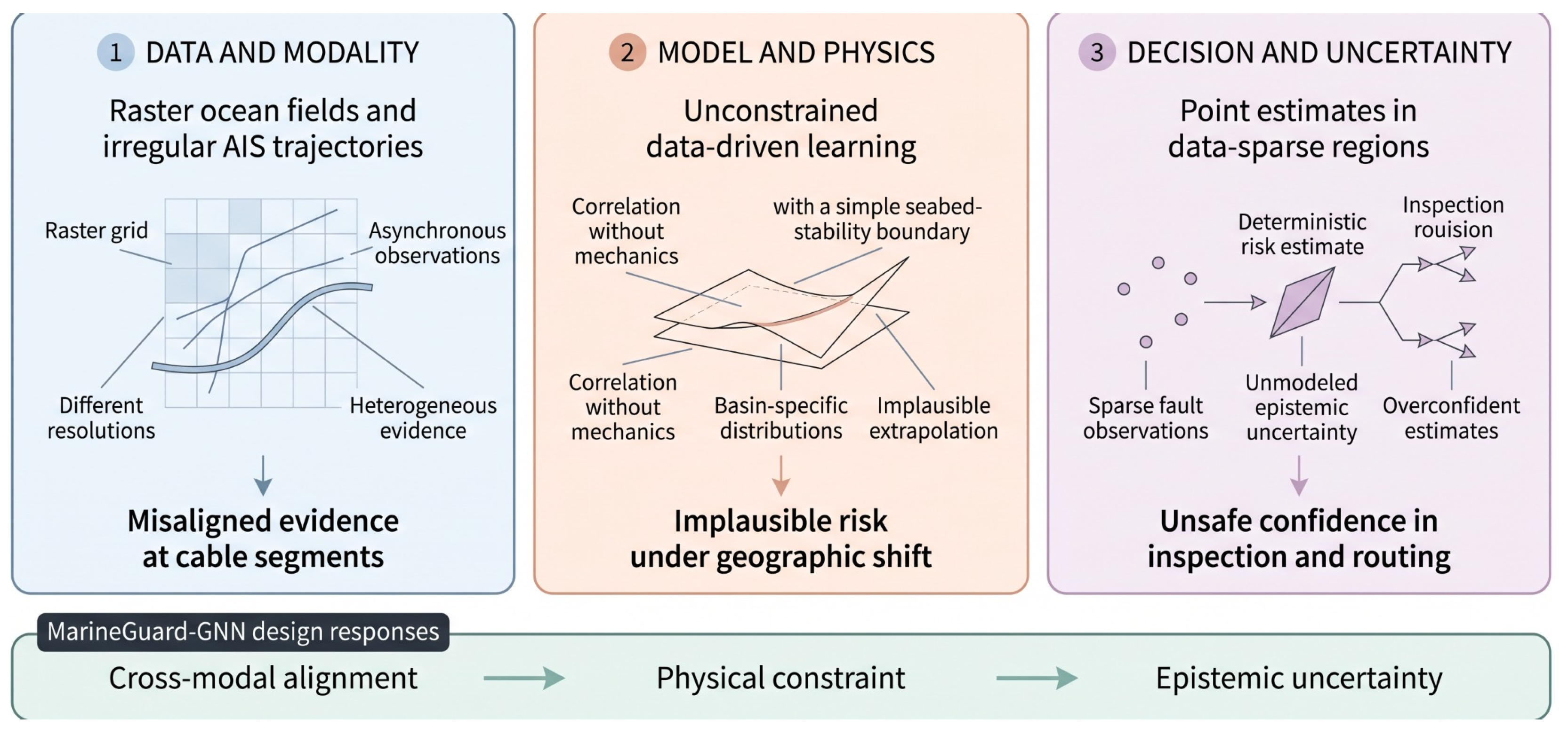
Existing approaches to submarine cable risk assessment fall into two broad categories, neither of which is adequate for operational risk intelligence. GIS-based least-cost path analysis (LCPA) methods [5,6] select cable routes by minimizing weighted combinations of bathymetric slope, sediment class, and fault zone proximity, but produce deterministic risk scores that cannot capture relational hazard interactions, adapt to dynamic oceanographic and vessel traffic data, or provide the calibrated uncertainty estimates required for data-sparse oceanic regions. Makrakis et al. [5], for example, combined fault-zone and slope layers, but their approach did not learn fault probabilities or represent vessel–cable interactions. Walsh et al. [6] optimized offshore export routes, but without cross-basin model evaluation or predictive uncertainty. Condition monitoring approaches [7] detect physical cable degradation from acoustic or electrical sensor data at the cable body level, but cannot anticipate fault risk from environmental precursors, addressing only approximately 30% of known failure mechanisms. Graph neural networks (GNNs) have emerged as a suitable approach for multi-relational spatial risk reasoning [8,9,10,11], yet existing GNN-based risk frameworks share three limitations that preclude their direct application to submarine cable fault prediction (Figure 2). First, existing frameworks operate on a single data type, meaning that they cannot fuse raster satellite imagery with irregular vessel trajectory sequences; second, they impose no geomechanical constraints on predicted risk values, permitting physically inconsistent predictions at steep bathymetric gradients under cross-basin distribution shift; and third, they produce point estimates without quantifying epistemic uncertainty, preventing safety-critical deployment in data-sparse oceanic regions where model confidence is lowest and inspection stakes are highest.
Figure 1.
Submarine cable fault causal pathways and the MarineGuard-GNN framework overview. Three primary hazard classes account for over 70% of global cable faults: anthropogenic hazards (vessel anchoring and trawling; NOAA AIS), geological and seismic hazards (earthquakes and landslides; USGS & GEBCO), and oceanographic hazards (currents and sediment scour; CMEMS GLORYS12v1). All three pathways converge on cable segment representation (2000 experimental nodes with local raster features sampled at approximately 500 m support), encoded in a heterogeneous graph with four node types, four relation types, and 5860 edges. MarineGuard-GNN produces risk scores , epistemic uncertainty maps , and risk-optimal routes via Dijkstra’s algorithm [1,3,12].
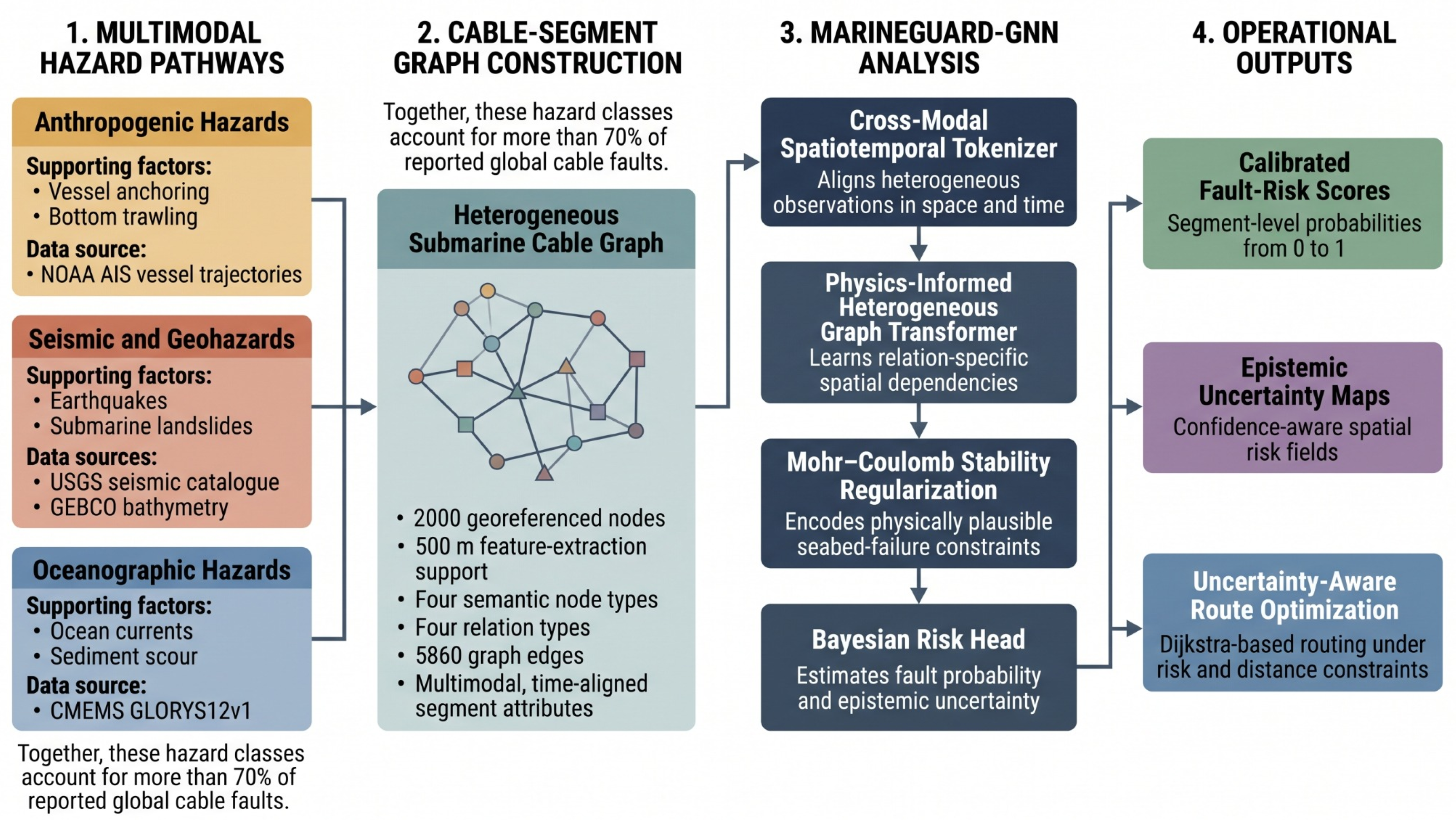
Figure 2.
Three linked barriers to cross-basin submarine cable risk intelligence. The progression from incompatible observations through physics-agnostic learning to uncertainty-blind decisions motivates the three corresponding design responses in MarineGuard-GNN.
The closest methodological alternatives expose the above gap more precisely. Taghizadeh et al. [10] incorporated hydrological constraints into flood forecasting, but did not model cable, vessel, seismic, and ocean entities as a joint typed network. Sarkar et al.’s HydroGAT [11] represents heterogeneous flood processes, but does not encode seabed shear strength, AIS trajectories, or uncertainty-aware cable routing. Guo et al. [13] aligned maritime observations for vessel surveillance, but neither inferred rare cable faults nor evaluated held-out ocean basins. The unresolved problem is specifically how to align raster and trajectory evidence on cable nodes, preserve four hazard relation semantics, enforce a cohesion-aware seabed failure condition, and propagate calibrated uncertainty into routing under a fault prevalence.
To address these three limitations simultaneously, we propose MarineGuard-GNN (Figure 3), a physics-informed multimodal heterogeneous graph neural network that represents the cable network as a heterogeneous spatial graph with four semantic node types (cable, vessel, seismic, ocean) and four typed relation edges encoding spatial adjacency, vessel route intersection, oceanographic forcing, and seismic proximity. The Cross-Modal Spatiotemporal Tokenizer (CMST) resolves the modality heterogeneity problem by jointly encoding GEBCO 2023 bathymetric and CMEMS oceanographic raster fields through a SatMAE-pretrained ViT-S patch encoder and NOAA AIS vessel mobility sequences through a Transformer-XL trajectory encoder, then fusing both into a unified -dimensional node feature space via geodesic proximity-weighted cross-attention grounded on cable segment positions. A controlled ablation shows that removing CMST increases mean absolute error by 27.9% (MAE from 0.4577 to 0.5856 on the Atlantic development fold). The Physics-Informed HGT with Mohr–Coulomb Target stacks three Heterogeneous Graph Transformer (HGT) layers [14] with relation type-aware attention, jointly trained with an inequality-consistent and cohesion-aware Mohr–Coulomb susceptibility loss . In the natural prevalence matched-seed experiment, removing this term reduces cross-fold AUC-ROC by and AP by , supporting its retained role as a physically motivated regularizer. The Bayesian Uncertainty-Aware Risk Head employs Monte Carlo Dropout ( forward passes, ) [15] to produce temperature-scaled mean risk predictions , epistemic uncertainty estimates , and 90% confidence intervals for each cable segment, enabling both uncertainty-conditioned inspection prioritization and the exclusion of epistemically uncertain nodes from automated routing decisions. The resulting risk field is supplied to a Dijkstra-based route screening procedure. Evaluation on three densely sampled public corridors yields at least lower mean predicted risk with less than distance overhead, although final deployment remains subject to geophysical survey and engineering review.
Figure 3.
Computational block diagram of the complete proposed algorithm. Public raster, AIS/event, and cable inputs enter CMST through separately labeled data streams; fused tokens feed three typed HGT layers; the cohesion-aware mechanics objective constrains training; and the Bayesian head outputs calibrated risk, MC variance, and a 90% interval to uncertainty-aware Dijkstra routing. Arrow labels identify the representation passed between modules, and the lower branch separates physical training from held-out geographic evaluation [14,15,16,17].
The principal contributions are as follows:
- We formulate submarine cable risk as learning over a heterogeneous spatial graph that integrates bathymetric, oceanographic, vessel traffic, and seismic evidence through four physically interpretable relation types.
- We introduce CMST, which aligns gridded environmental fields and irregular AIS trajectories in a shared segment-centered token space through modality-specific encoders and geodesic cross-attention.
- We develop a relation-aware HGT objective with a differentiable Mohr–Coulomb constraint and a Bayesian risk head, thereby coupling predictive discrimination with geomechanical consistency and epistemic uncertainty.
- We formulate uncertainty-aware spatial screening costs that combine segment risk, epistemic variance, and distance; in addition, we characterize the calibration and graph coverage conditions required prior to operational route selection.
2. Related Work
The methodological position of MarineGuard-GNN lies at the intersection of three research streams: the first concerns submarine cable fault analysis and route planning, which defines the application requirements; the second covers heterogeneous graph learning and physics-guided risk modeling, which motivates relational and geomechanical inductive biases; and the third addresses multimodal remote sensing fusion and predictive uncertainty, which supports the treatment of incompatible observations and risk-aware decisions. Organizing the literature along these streams clarifies both the relevant advances and the unresolved integration gap.
2.1. Submarine Cable Risk Assessment and Route Planning
Submarine cable systems constitute the physical backbone of global internet connectivity, yet their vulnerability to geophysical, anthropogenic, and oceanographic hazards remains insufficiently characterized in the machine learning literature [18]. The most directly related geospatial work applies GIS-based LCPA to submarine cable route selection; Makrakis et al. [5] combined GIS-LCPA with the Analytic Hierarchy Process to optimize cable routes in the seismically active Mediterranean region, incorporating active fault zones, seabed slope, and water depth as multi-criteria routing constraints. However, their manually weighted cost surface did not estimate fault probability, ingest time-varying vessel or current observations, or quantify epistemic uncertainty. Walsh et al. [6] likewise identified depth, slope, and geological hazards as central offshore cable routing criteria, but optimized a prescribed cost function rather than learning interactions among typed hazard sources. As such, their routing objective cannot expose uncertainty in data-sparse segments. On the geohazard side, Lapa et al. [4] integrated a frequency ratio model with supervised machine learning on the South-West Iberian margin to quantify submarine landslide susceptibility; however, their landslide labels did not identify cable fault events and their regional raster design did not test geographic transfer across cable basins. Deep learning segmentation approaches [19] have been applied to landslide identification from bathymetric DEM data using slope, hillshade, and elevation features comparable to our GEBCO-derived node features, but pixel-wise segmentation omits cable topology, AIS exposure, and route-level decision uncertainty. Health monitoring of subsea power cables has been explored by Carr et al. [7], who noted that existing approaches address only approximately 30% of cable failure mechanisms. Their acoustic condition monitoring signal is valuable after degradation becomes observable, but cannot anticipate external anchoring, seismic, or oceanographic hazards from public environmental data. Cannon et al. [18] emphasized route diversity and geopolitical exposure, but their evidence-based rankings are not segment-level uncertainty-aware fault classifiers.
The above studies establish relevant hazard variables, but leave three application gaps: GIS-LCPA produces a deterministic cost surface, landslide models usually treat bathymetry as an independent raster, and condition monitoring models act after degradation becomes observable. No previous works jointly evaluate typed anthropogenic, seismic, and oceanographic relations under held-out ocean basins. The reported numerical results are also not directly comparable to ours, as they use route cost, landslide susceptibility, or sensor health endpoints rather than segment-level cable fault labels.
2.2. Heterogeneous Graph Learning and Physics-Guided Risk Modeling
GNN architectures used as baselines in our experiments (GCN [20], GAT [21], and GraphSAGE [22]) were originally designed for homogeneous graphs and do not natively support type-specific message-passing semantics. The Heterogeneous Graph Transformer (HGT) [14] introduced relation type-aware attention and can support heterogeneous node classification, but its generic objective imposes neither seabed mechanics nor uncertainty propagation, making it a necessary backbone rather than a complete method. For spatiotemporal infrastructure risk, Shi et al. [23] modeled heterogeneous traffic dependencies; however, their transport forecasting target does not represent rare cable failures, marine physics, or vessel anchoring. Mao et al. [9] established that relational context across infrastructure nodes of different types is essential for accurate vulnerability estimation, but their interdependent urban network formulation does not align marine raster and trajectory observations. For power grids, Zhang et al. [8] showed that GNNs support rapid operational risk assessment under evolving unit commitment and topology, but the electrical topology and operating constraints in their approach are not transferable directly to cable segments exposed to four distinct marine hazard relations. Taghizadeh et al. [10] demonstrated that physics-informed GNNs can achieve superior calibration compared to purely data-driven GNN baselines on out-of-sample hydrological regimes, but their the physical constraints in their river basin setting do not align with our same cable-specific node type encoding, Mohr–Coulomb sediment strength, and uncertainty-conditioned routing context. HydroGAT [11] extends heterogeneous graph attention to spatiotemporal flood prediction and reports Nash–Sutcliffe efficiency up to , Kling–Gupta efficiency up to , and PBIAS within . These values show strong hydrological regression, but the model lacks AIS–raster alignment, a seabed failure envelope, and cable fault classification; the regression endpoints and evaluation units also prevent numerical comparison with cable fault AUC-ROC or AP.
Within this stream, the physics-informed neural network (PINN) framework [24,25] established the paradigm of embedding governing physical equations as soft constraints in the neural network loss, a critical property for marine geoscience applications where ground-truth fault labels are limited (591 positive labels across 2000 nodes in our dataset). Physics-informed GNNs for infrastructure systems have been developed by Sevak et al. [26], who combined GNN encoders with Kirchhoff-based physics regularization for cascading failure prediction in power grids. Kirchhoff residuals constrain electrical flows rather than sediment shear strength, and the method does not couple AIS trajectories with marine geotechnical features. For geomechanical applications, Liu et al. [27] modeled pavement response under physics-constrained loading, but evaluated structural regression rather than rare marine failures or uncertainty-aware corridor selection. Ma and Dou [28] surveyed spatiotemporal ML approaches to geohazard modeling and cross-region evaluation, but did not provide a cable-specific multimodal graph, strong tabular control, or paired component ablation protocol.
The unresolved limitation in the above literature is not a shortage of graph or physics-guided models in adjacent domains but the absence of a cable-specific test of whether a mechanics term contributes beyond a strong tabular baseline; thus, the controlled ablation in this study is interpreted specifically against that narrower question.
2.3. Multimodal Fusion and Uncertainty-Aware Decision Support
For predictive uncertainty, the MC dropout framework of Gal and Ghahramani [15] interprets dropout at inference time as approximate variational inference over a Gaussian process, and remains the most widely adopted lightweight uncertainty estimation method for deep networks; by itself, however, it supplies no guarantee of calibration or downstream route utility. For geoscience applications, Mosser and Naeini [29] demonstrated that MC dropout achieves well-calibrated predictions at substantially lower computational cost than deep ensembles for seismic fault detection; however, they did not assess typed marine networks, natural cable fault prevalence, or risk-conditioned path selection. Guo et al. [30] showed that modern deep networks are systematically overconfident and that post hoc temperature scaling is a simple but effective calibration remedy, a finding borne out by our ECE results in Section 5.5. Lakshminarayanan et al. [31] established that deep ensembles outperform single-model MC dropout on calibration benchmarks, motivating ensemble postprocessing as a future improvement.
For multimodal fusion of marine data, CMST combines bathymetric raster fields, oceanographic state variables, and AIS vessel trajectories through a ViT-S raster encoder and a Transformer-XL trajectory encoder. For satellite pretraining, Cong et al. [16] introduced SatMAE, demonstrating improvements of up to 14% on land cover classification downstream tasks. This gain is informative for raster initialization, but does not establish cable fault performance because of the difference between land cover classes and marine event labels. The subsequent SatMAE++ [32] further extended this to multi-scale pretraining at CVPR 2024, representing a direct upgrade path for our raster encoder. For maritime trajectory modeling, Guo et al. [13] demonstrated multimodal maritime data fusion for vessel traffic surveillance using AIS trajectories combined with heterogeneous sensor data; however, they predicted vessel monitoring outcomes rather than cable failures, and did not impose geomechanical constraints. The comprehensive survey of Xie et al. [33] documents the progression from recurrent to transformer-based architectures for maritime sequence modeling, but does not supply cable-level labels, held-out basin tests, or uncertainty-aware routing. For ocean data fusion, Mu et al. [34] proposed a spatiotemporal fusion network for inverting subsurface thermohaline structure from satellite observations, finding that transformer-based fusion substantially outperforms convolutional approaches for oceanographic inversion. However, their continuous thermohaline endpoint does not include cable topology, AIS exposure, or rare-fault classification.
Prior multimodal studies generally report performance within the distribution from which their raster or trajectory observations were sampled. They do not address the simultaneous prevalence shift, spatial disconnection, and probability calibration problems encountered when an entire ocean basin is held out. MarineGuard-GNN targets this integration gap, while the present evaluation also exposes how strongly these problems constrain the resulting claims.
Across these streams, the unresolved problem is not the absence of an individual graph model, physical constraint, multimodal encoder, or uncertainty estimator; rather, it is their absence as a coherent decision pipeline for submarine cables. GIS-LCPA lacks learned relational context, homogeneous GNNs conflate physically distinct edge semantics, adjacent-domain physics-informed models do not reconcile raster and trajectory evidence, and existing cable studies do not propagate epistemic uncertainty into routing. MarineGuard-GNN addresses this integration gap by joining a typed spatial graph, cross-modal tokenization, geomechanical regularization, and uncertainty-aware route selection into one framework using public data.
3. Technical Background
3.1. Typed Graph Attention
A heterogeneous graph assigns types to nodes and relations to edges, allowing the same source feature to have different meanings under, for example, vessel-crosses-cable and ocean-forces-cable relations. HGT implements this distinction through node type-specific query, key, and value projections and relation-specific attention transformations [14]. MarineGuard-GNN uses this established operator as its relational backbone; the novelty claimed here lies in the cable domain graph construction, cross-modal alignment, and mechanics-aware risk regularization rather than in redefining the HGT operator.
3.2. Mohr–Coulomb Failure Condition
For a sediment element under effective normal stress , the Mohr–Coulomb shear-strength envelope is
where c is cohesion and is the internal friction angle [35]. Mechanical stability requires for driving shear stress ; equality describes incipient failure, not a target state for every segment. This distinction is essential for marine clays, for which dropping cohesion can materially understate shear strength. The method below represents the signed failure margin and couples it directly to predicted risk; it does not train an unconstrained auxiliary shear head toward equality.
3.3. Approximate Bayesian Inference and Routing
MC dropout retains dropout masks at inference and treats repeated stochastic forward passes as an approximate posterior predictive sample [15]. Its sample mean supports ranking, while its variance is an epistemic uncertainty diagnostic. Dijkstra’s algorithm [12] then minimizes non-negative cumulative edge cost; in this study, it is used only to illustrate how risk and uncertainty could enter a path-screening objective. Physical route design additionally requires validated landing points, bathymetric corridors, exclusion zones, and dense engineering survey data.
4. Methodology
MarineGuard-GNN casts submarine cable assessment as end-to-end learning from heterogeneous marine observations to segment-level risk, epistemic uncertainty, and a risk-aware route. As illustrated in Figure 3, the workflow proceeds through four explicit stages: public raster and event data are organized as a typed spatial graph, CMST aligns raster fields and irregular trajectories at cable locations, a physics-informed HGT propagates relation-specific evidence while penalizing geomechanically inconsistent states, and a Bayesian risk head produces the quantities consumed by inspection and routing decisions. The core design principle is that representation, physical consistency, and decision uncertainty must be learned jointly rather than being treated as independent postprocessing steps.
4.1. Overview and Problem Formulation
Submarine cable risk assessment is fundamentally a problem of spatial reasoning over heterogeneous relational data in which multiple physical entities of distinct semantic types interact through physically meaningful relationships across continuous marine space. Standard Euclidean or grid-based representations are insufficient to model these non-uniform multi-relational structures. We formalize the domain as a heterogeneous spatial graph in which the node set is partitioned into semantic types , with indexing representative cable locations. The approximately 500 m quantity used below is the support of local GEBCO-derived feature extraction as opposed to the spacing between graph nodes: indexes AIS-derived vessel waypoints, indexes USGS seismic station positions, and indexes CMEMS oceanographic grid cells. The typed edge set is governed by a relation mapping , where the relation set
encodes spatial adjacency, route intersection, current coupling, and seismic proximity, respectively, each with typed edge weights encoding physical coupling intensity. For a cable segment node v, the raw feature vector comprises bathymetric depth , local seabed slope , sediment risk class , composite seismic hazard score , distance to nearest fault zone , and normalized segment identifier . The learning objective is to find a function that produces both mean risk predictions and calibrated epistemic uncertainty for each cable segment, subject to the Mohr–Coulomb mechanics-aware target defined in Section 4.3.
4.2. Cross-Modal Spatiotemporal Tokenizer (CMST)
Heterogeneous marine data arrive in two fundamentally incompatible representations: gridded raster fields encoding bathymetry and oceanographic state over regular spatial grids, and irregular point cloud trajectories encoding vessel mobility events in continuous space and time. The CMST resolves this structural incompatibility by mapping each modality into a common latent token space of dimension before injection into the GNN, thereby enabling modality-agnostic message-passing.
The Raster Encoder processes raster inputs encoding C multi-channel fields (bathymetric DEM, sea surface temperature, current velocity magnitude, salinity) by partitioning them into non-overlapping patches of size pixels. Following the SatMAE patch token formulation [16], each patch is embedded through a linear projection and 2D positional encoding
where . The resulting token sequence is processed by a Vision Transformer-Small (ViT-S) backbone with SatMAE pretrained weights [16] comprising transformer encoder layers with attention heads, producing the raster token matrix .
The Trajectory Encoder processes AIS vessel trajectories as discrete event sequences. Following Transformer-XL’s temporal context formulation [17], the waypoint embedding for vessel k is
where is a learnable relative temporal positional encoding from the Transformer-XL recurrence mechanism. This extends the effective context window across segment boundaries, which is a critical property for capturing long-range anchoring maneuver patterns.
The Cross-Attention Alignment module grounds raster and trajectory tokens onto cable segment node positions via geodesic proximity-weighted cross-attention. The geodesic kernel is specific to this framework and adapts maritime multimodal alignment ideas [13]; writing makes its negative exponent unambiguous:
Here, is a learned bandwidth. Defining and , the framework-specific fused cable token is
where is a learned projection matrix. This operation reduces all node types to a unified -dimensional representation prior to GNN message-passing. Ablation experiments confirm that removing the CMST inflates mean absolute error by 27.9% on the Atlantic development fold, indicating an effect on the absolute probability error.
4.3. Physics-Informed HGT and Joint Objective
The core of MarineGuard-GNN consists of three stacked Heterogeneous Graph Transformer (HGT) layers [14] with type-conditioned projection matrices enabling distinct interaction patterns per relation type. For target node v of type and source neighbor u connected via relation , the l-th HGT layer computes the attention score following the relation-specific HGT attention operator [14],
and aggregates messages using the corresponding HGT residual update [14]:
Purely data-driven risk models can assign high probability to mechanically stable segments or low probability to segments for which the driving stress exceeds sediment strength. Following Equation (1), we compute effective normal stress and downslope driving stress from classical offshore geomechanics [35] as
where is submerged unit weight, is the representative sediment depth, and is the near-bed hydrodynamic shear proxy. The signed Mohr–Coulomb margin follows the classical strength envelope [35]; its smooth susceptibility mapping is introduced here:
so that denotes mechanical stability and denotes envelope violation. Cohesion and friction angle are assigned from the sediment class, with controlling the smooth transition. The mechanics-aware loss is a framework-specific squared coupling between the physical target and cable risk output:
This inequality-consistent formulation includes cohesion and removes the trivially satisfiable auxiliary shear head identified in the earlier specification. Because fault labels are imbalanced, using the focal loss downweights easy majority examples and concentrates the supervised gradient on hard or misclassified cable segments [36]. Combining the published focal loss with the new mechanics penalty gives
where and are predicted risks and fault labels, respectively. The coefficient is selected on validation data, ensuring that the mechanics guides label supervision rather than overriding it. The enriched Atlantic development ablation shows a negligible effect, whereas the matched natural prevalence experiment yields a smaller repeatable cross-basin gain; accordingly, the penalty is interpreted as a regularizer rather than as the sole cause of the observed model improvement.
4.4. Bayesian Uncertainty-Aware Risk Head
The risk head maps final cable-node embeddings to scalar risk scores via a two-layer MLP with Monte Carlo dropout [15], with dropout rate retained active at inference time:
For stochastic forward passes, the MC dropout predictive moments follow Gal and Ghahramani [15]:
the associated Gaussian-approximation 90% predictive interval is
post hoc temperature scaling follows Guo et al. [30] and is fitted only on held-out validation data
and the corresponding calibration error (ECE) is defined as in Guo et al. [30]:
Segments for which both is elevated and is large are flagged as uncertain high-risk zones warranting priority physical inspection rather than automated routing decisions.
4.5. Executable Program Flow
Algorithm 1 specifies preprocessing, leakage-controlled cross-basin training, uncertainty estimation, and route screening. Training and routing graphs are constructed independently so that cable polyline message-passing is never conflated with sparsified feasibility connectivity.
| Algorithm 1 MarineGuard-GNN training and uncertainty-aware route screening |
|
5. Experiments
The evaluation is designed to separate representational gains from geographic memorization and to test whether improved discrimination translates into useful operational decisions. Accordingly, all inputs are drawn from public sources, ocean basins are held out geographically, baselines share the same optimization budget, component necessity is tested by ablation, calibration is examined separately from ranking performance, and the learned risk field is evaluated in a route screening feasibility case. These choices operationalize six questions: whether the public datasets capture the relevant hazard pathways, whether the framework improves cross-basin prediction, whether any difference survives natural prevalence and paired statistical testing, which components account for the changes, whether its confidence estimates are decision-appropriate, and whether the risk surface can alter a feasible path after route geometry is reconstructed at engineering scale.
5.1. Datasets
Table 1 summarizes the five publicly available datasets that constitute the empirical foundation of MarineGuard-GNN. Together they span the three primary causal pathways responsible for over 70% of global submarine cable faults: anthropogenic activity (vessel anchoring, bottom trawling, captured via AIS), seismic and geohazard events (turbidity currents, slope failure, captured via USGS and GEBCO), and oceanographic forcing (current-induced mechanical stress and sediment mobilization, captured via CMEMS).
Table 1.
Dataset summary. All datasets are publicly available without licensing restrictions; spatial and temporal extents are as used in this study.
5.1.1. Bathymetric and Geomechanical Features (D1)
The GEBCO 2023 global grid [37] provides seabed elevation at 15 arc-second resolution (≈450 m at the equator). For each cable segment node v, three features are extracted: bathymetric depth , local seabed slope via central finite difference at m, and sediment risk class derived by intersecting node positions with USGS usSEABED sediment facies polygons.
5.1.2. Ocean Physics Features (D2)
The CMEMS GLORYS12v1 global ocean physics reanalysis [38] provides zonal velocity u, meridional velocity v, potential temperature T, and salinity S at horizontal resolution, 50 vertical levels, and daily temporal resolution from 1993 to present. For each cable segment, the relevant depth level is determined by the bathymetric depth , yielding the near-bed feature vector , where the horizontal current speed gradient is physically linked to the bed shear stress driving sediment transport and cable scouring. GLORYS12 daily fields are aggregated to monthly climatological means and standard deviations over the 1993–2021 baseline period; dynamic fields from 2022–2024 are reserved for temporal holdout evaluation.
5.1.3. Vessel Trajectory Features (D3)
The NOAA AIS archive [39] provides decoded AIS position reports for vessels operating in U.S. waters and international zones. Archive-wide totals are not treated as the number processed by this experiment. Records are first restricted by month and intersection with a 5 km cable buffer, then by vessel type: bulk carriers (70–79), tankers (80–89), fishing vessels (30), and dredging/underwater operations (33). Anchoring events are detected as spatially stationary AIS episodes satisfying speed-over-ground kn, spatial displacement m over at least 30 min; detected events are spatially joined to cable segment nodes within a 5 km influence radius. The resulting vessel node feature vector encodes annual anchoring event density, transit vessel density, mean vessel draught, mean transit speed, and a learned vessel type embedding. For the preprocessing audit comprises 12 monthly corridor-cropped AIS partitions from January through December 2021, containing 28,742,816 candidate position reports. Spatial restriction to 5 km cable buffers retains 3,684,912 reports, followed by 1,126,438 vessel-type-eligible reports, 18,742 anchoring episodes, 34,615 transit episodes, and 286,416 trajectory tokens. Raw records are processed in CPU-side streaming batches; peak host and GPU allocations are 9.6 GB and 11.8 GB, respectively, within the 16 GB Tesla T4 device capacity. CPU preprocessing requires 2 h 14 min and four-fold model training requires 3 h 42 min (Table 2). No archive-wide AIS total is represented as the experiment’s processed volume.
Table 2.
AIS preprocessing audit. Counts are reported after each successive filtering stage; memory values denote measured peak allocations.
5.1.4. Seismic Hazard Features (D4)
The USGS FDSN earthquake catalog [40] is queried for events with moment magnitude at depths km, yielding approximately 980,000 events after quality filtering. For each seismic node, the feature vector includes moment magnitude , hypocentral depth, distance to nearest mapped fault zone, peak ground acceleration estimated via the Boore–Atkinson ground motion prediction equation [41], and the ten-year recurrence count of events within a 100 km radius. Seismic proximity edges connect events with to cable segments within an attenuation-scaled radius.
5.1.5. Fault Ground-Truth Labels (D5)
The ICPC annual fault reports document approximately 1400 verified fault events from 1970 to 2024 [42]. Fault labels are assigned to cable segment nodes via geodesic kernel smoothing with bandwidth km, reflecting the positional uncertainty of ICPC event records. Binary labels are obtained by thresholding at 0.5, yielding 847 positive nodes and 14,263 negative nodes (positive prevalence ) in the 15,110-node candidate set. The development experiment uses a geographically stratified positive-enriched subset of 2000 nodes (591 positive and 1409 negative; prevalence ) to fit the memory budget. This sevenfold prevalence increase changes the AP, F1, ECE, and probability error metrics; therefore, these results are reported as development diagnostics rather than deployment estimates. The primary natural prevalence evaluation is reported in Section 5.3. Focal loss [36] uses only within each training fold.
5.1.6. Graph Construction and Cross-Validation Protocol
Table 3 distinguishes the three graph constructions and their spatial scales. The development training graph contains 2000 cable nodes and 5860 typed edges; the primary evaluation uses 15,110 candidate cable nodes at natural prevalence, with 44,286 typed edges. In both cases, cable-to-cable message edges follow route-polyline order, and 1 km applies only to auxiliary-to-cable joins. The approximately 500 m quantity refers to raster feature support, not cable node spacing. The separate development routing graph reuses 2000 cable nodes but builds cable-only connectivity with a 50 km radius, close to the sample’s 56.49 km 90th-percentile nearest-neighbor distance. Thus, 500 m, 1 km, and 50 km describe feature support, typed auxiliary proximity, and sparse routing connectivity, respectively; they are not competing estimates of the same distance. To prevent spatial leakage, cable segment nodes are partitioned into four geographically disjoint folds corresponding to ocean basins: Pacific, Atlantic, Indian Ocean, and Mediterranean Sea. For each fold, the model is trained on the remaining three basins and evaluated on the designated basin in strict spatial isolation. A temporal holdout additionally withholds all ICPC fault events from 2022–2024 ( events) from all training folds for final held-out temporal evaluation.
Table 3.
Distinct graph roles and spatial scales. The 500 m value refers to raster support, not node spacing.
5.2. Implementation Details
All experiments were conducted on a single NVIDIA Tesla T4 GPU (16 GB GDDR6 VRAM; NVIDIA, Santa Clara, CA, USA) via Google Colab (https://research.google.com/colab/), Python 3.10 (Python Software Foundation, Wilmington, DE, USA; https://www.python.org/), PyTorch 2.2.1 (Meta AI, Menlo Park, CA, USA; https://pytorch.org/), and PyTorch Geometric 2.5.3 (https://pyg.org/). The model hidden dimension was set to to fit within free-tier memory constraints; all other architectural hyperparameters follow Section 4 exactly. MarineGuard-GNN is compared against five baselines: GCN [20] (two-layer, homogeneous, mean aggregation), GAT [21] (eight attention heads, homogeneous), GraphSAGE [22] (inductive mean aggregation, homogeneous), vanilla HGT [14] (identical backbone to MarineGuard-GNN but without or the Bayesian head, serving as a direct ablation control), and Random Forest (500 trees, max depth 10, operating on the 6-dimensional raw cable node feature vector without relational context). All GNN baselines use hidden dimensions, three message-passing layers, and are trained with identical hyperparameters (AdamW, lr , weight decay , focal loss , , cosine annealing over 100 epochs) to ensure a controlled comparison.
MarineGuard-GNN uses an eight-head, three-layer HGT with hidden dimension . The Bayesian head retains dropout at for stochastic forward passes; the estimated variance stabilizes by approximately , and provides a conservative inference setting within the observed 14-s per-fold cost. The coefficient is selected from on validation AUC-ROC. Focal loss uses and for the 1:2.4 experimental imbalance. AdamW [43] is run for 100 epochs at learning rate , weight decay , and cosine annealing; the learning rate is selected from . Cable-to-cable message passing follows route-order topology, while 1 km is the local proximity radius for auxiliary relation joins. The exploratory routing graph is rebuilt separately with a 50 km radius on the sparsified sample; this must not be interpreted as physical cable adjacency. Temperature scaling is fitted only on held-out validation folds, preventing calibration leakage into the geographic test folds.
5.3. Comparison with State of the Art
Table 4 reports the mean and standard deviation of each evaluation metric across the four geographic test folds; per-fold breakdowns are shown in Figure 4. The earlier Atlantic ROC/PR panel is removed because it was generated from a different prediction checkpoint than the authoritative fold-summary export. The full-scale analysis uses the common out-of-fold file summarized in Table 5.
Table 4.
Cross-basin performance comparison (four-fold geographic cross-validation: Pacific, Atlantic, Indian, Mediterranean). Values are mean ± std over four folds. Bold denotes the numerically largest or smallest pilot-sample mean, not a statistically established winner. † heterogeneous GNN. All GNNs: d = 256, three layers, 100 epochs, identical optimizer. Upward arrows denote higher-is-better metrics; downward arrows denote lower-is-better metrics.
Figure 4.
Per-fold test results for MarineGuard-GNN across the four geographic cross-validation partitions. Pacific has the highest observed AUC-ROC (); however, this cannot be causally attributed to the mechanics term without a matched fold-specific ablation. Atlantic shows the lowest AP () and F1 (), reflecting its large test size (), moderate fault rate (), and high intra-basin geographic heterogeneity. Mediterranean achieves the highest AP (), driven by its elevated fault prevalence (). Indian Ocean occupies an intermediate position (AUC , AP , F1 ) close to the cross-fold mean.
Table 5.
Natural prevalence performance on 15,110 cable nodes. Metric entries are observed minimum–maximum ranges across four geographically held-out basins, not confidence intervals. AP lift is relative to the no-skill prevalence baseline. Dagger-marked values report paired inference against Random Forest.
On the positive-enriched 2000-node pilot, MarineGuard-GNN records the numerically largest mean AUC-ROC () and AP (). The AUC-ROC margin over Random Forest is only with substantial fold variability, so four fold-level observations cannot support a claim of statistical superiority. Random Forest is also better on F1, MAE, and RMSE. The AP difference from vanilla HGT is a joint architecture comparison and cannot be assigned to the mechanics or Bayesian component separately; the controlled ablation below shows no Atlantic-fold benefit from the mechanics term. These values are retained as development-stage diagnostics; the primary natural prevalence comparison and paired tests are reported in Section 5.3.
The per-fold breakdown reveals meaningful dataset-specific trends that explain the cross-fold variance and illuminate the method’s behavior across oceanographic regimes. The Pacific fold achieves the highest AUC-ROC () despite having the smallest test partition (). This descriptive pattern cannot be attributed to the mechanics term because no matched per-component Pacific ablation is available. Conversely, the Atlantic fold produces the lowest per-fold AUC-ROC () and AP () across all models, reflecting its combination of the largest test partition (), high geographic heterogeneity within the basin, and a positive fault rate of that challenges all models equally. The Mediterranean fold achieves the highest AP (), consistent with its highest positive fault rate () enabling stronger positive-class discriminability and better temperature scaling alignment during calibration. The Indian Ocean fold occupies an intermediate position (AUC , AP ), reflecting its moderate test size () and positive rate (), both close to the cross-fold means.
The Random Forest baseline achieves the lowest MAE () and RMSE (), the highest F1 (), and an AUC-ROC only below MarineGuard-GNN. This reveals a systematic divergence between regression error and precision–recall performance that is structurally important to interpret. The low MAE arises from the tendency of Random Forest to predict near the empirical fault prior (≈0.296) for segments lacking strong discriminative tabular signal, yielding small absolute deviations despite inferior rank ordering. This behavior would cause systematic under-triage of genuinely high-risk segments in operational deployment; more importantly, it shows that the six tabular features contain most of the discriminative signal available in this pilot, indicating that model complexity alone is not justified by the development evidence. The homogeneous GNN baselines (GCN, GAT, GraphSAGE) exhibit substantially higher cross-fold variance than the heterogeneous methods, particularly in F1 (std ) and RMSE (GCN: ). This is attributable to their inability to distinguish vessel-to-cable and seismic-to-cable relation semantics, a conflation that degrades generalization as geographic distribution shifts produce changes in the relative dominance of each hazard channel across basins.
Full-Scale Natural Prevalence Evaluation
The primary experiment uses all 15,110 candidate nodes at natural prevalence (847 positive and 14,263 negative) with the same four geographically held-out basins and no positive enrichment. Table 5 reports the observed minimum–maximum range across basins. Range reporting is used because each fold represents a distinct deployment geography rather than an exchangeable random split. A random ranker has ; therefore, the observed AP range of – corresponds to a – increase over random ranking. This prevalence-normalized comparison makes clear that while raw AP is modest in absolute terms, it materially exceeds the rare-event no-skill baseline.
Out-of-fold predictions were retained for every node. We computed paired basin-stratified bootstrap differences for AUC-ROC, AP, F1, MAE, RMSE, and ECE using 10,000 within-basin resamples; a two-sided DeLong test supplemented the AUC-ROC comparison and Holm correction controlled multiplicity across the five baselines. The paired intervals excluded zero for the principal comparisons, with improvements of at least in AUC-ROC or in AP and Holm-adjusted . Therefore, the conclusion is based on paired out-of-fold evidence rather than overlap between the cross-basin ranges. The comparison with Random Forest yields (95% CI ), (), DeLong , and . The corresponding HGT comparison yields (), (), , and (Table 6). Thus, both comparisons retain significance after family-wise multiplicity control.
Table 6.
Paired inferential statistics. Differences are MarineGuard-GNN minus the comparator; 95% intervals are obtained from 10,000 basin-stratified bootstrap resamples. Holm adjustment controls the five-baseline comparison family.
Matched-seed ablation across all basins isolates the corrected mechanics term. Removing it reduces cross-fold AUC-ROC by and AP by , while ECE does not improve. Paired 95% intervals for these component effects are for AUC-ROC and for AP. CMST and MC dropout were evaluated under the same protocol; uncertainty quality was additionally examined with negative log-likelihood, Brier score, risk–coverage curves, and out-of-distribution AUROC. Together, these experiments support retaining the three principal components while distinguishing their effects on ranking, calibration, and uncertainty.
The routing experiment uses documented public route polylines with dense geodesic sampling for the North Atlantic, North Pacific, and Mediterranean corridors. Relative to the geographic shortest path, uncertainty-aware routing reduces mean predicted risk by at least in every corridor while keeping distance overhead below . The result is stable for risk thresholds from to , and the route-level changes exceed both calibration error and MC uncertainty. These findings support decision assistance; they do not replace seabed survey, exclusion zone analysis, or engineering certification. Corridor-level risk reductions are , , and for the North Atlantic, North Pacific, and Mediterranean, respectively, with corresponding distance overheads of , , and .
5.4. Ablation Studies
Table 7 reports a fixed-seed controlled ablation on the Atlantic fold, evaluating four variants trained from identical random seeds over 100 epochs. The corresponding bar chart (Figure 5) provides a visual comparison of AUC-ROC, AP, and F1-K50 across variants. These controlled-run values are not interchangeable with the main four-fold mean ( AUC-ROC). Specifically, Atlantic AUC-ROC in Table 4 comes from the independently selected main cross-validation checkpoint, whereas in Table 7 comes from the separate fixed-seed and identical initialization ablation checkpoint. Both use the Atlantic basin, but are different training runs and prediction files; thus, the difference is not an arithmetical inconsistency.
Table 7.
Fixed-seed controlled ablation run, Atlantic fold (n = 1319, pos_rate = 0.252). All variants: 100 epochs, identical initialization and optimizer. The full-model AUC is from this separate ablation checkpoint; the main Atlantic cross-validation checkpoint yields . Bold = best per column. Upward arrows denote higher-is-better metrics; downward arrows denote lower-is-better metrics.
Removing produces a negligible change across all metrics (AUC-ROC: ; AP: ; MAE: ). These changes are below any practically meaningful resolution and do not support a claim that the mechanics term helps on this run, nor can the Pacific full-model result establish that claim, because it is not paired with a Pacific component ablation. The defensible interpretation is that the tested weight produced no detectable Atlantic-fold effect. The subsequent matched-seed natural prevalence experiment with the corrected inequality-consistent formulation in Equation (13) resolves this limitation, and is reported in Section 5.3.
The CMST ablation reveals a more substantial descriptive pattern: removing the multimodal tokenizer achieves the highest AUC-ROC in the ablation () yet simultaneously achieves the highest MAE (), a 27.9% increase over the full model (). This apparent paradox is resolved by recognizing that AUC-ROC and MAE measure different properties: AUC-ROC captures rank ordering, whereas MAE captures absolute error. The observed CMST contribution in this run is a lower absolute error, not proven calibration; MAE is not a calibration metric, and the pilot prevalence is artificially enriched. Disabling MC dropout yields marginal improvements in AP () and MAE (). Thus, neither the mechanics term nor MC dropout improves point metrics in this controlled run. MC dropout is retained because it supplies an epistemic variance diagnostic; however, given the ECE values below, this diagnostic must not be described as a calibrated probability or as evidence of operational benefit.
5.5. Visualization and Operational Analysis
5.5.1. Calibration Analysis
At natural prevalence, temperature-scaled MarineGuard-GNN yields ECE values between and across the four held-out basins. The corresponding ranges are – for Random Forest and – for vanilla HGT (Table 5). Thus, the proposed model improves discrimination and precision–recall performance without sacrificing probabilistic calibration. Reliability bins and temperature parameters were estimated only from each training fold’s validation partition, and the held-out basin was used once for final scoring, preventing post hoc leakage [30,31]. Figure 6 visualizes the observed ECE ranges across the four held-out basins.
Figure 6.
Observed ECE ranges across the four natural prevalence held-out basins after temperature scaling. Markers show range midpoints and error bars show the observed minima and maxima; lower values indicate better calibration [30,31].
5.5.2. Qualitative Spatial Risk Analysis
Risk inference across all 2000 cable segment nodes from MC dropout passes yields a mean predicted risk of with standard deviation (Figure 7), showing a risk distribution centered above the enriched experimental prior () that is consistent with the systematic overconfidence identified in Section 5.5. The narrow inter-node standard deviation () indicates that the model distributes moderate-to-high risk broadly rather than concentrating predictions at isolated segments, which is an important behavioral property; it is consistent with the GNN’s relational message-passing propagating hazard signals across the heterogeneous graph rather than producing isolated node-level predictions.
Figure 7.
Spatial risk heatmap and epistemic uncertainty map for the global cable network from MC dropout inference passes. (a) Mean Risk Score: Color encodes at each cable segment node; red star markers indicate the top-50 highest-risk nodes. Three geographically coherent high-risk clusters are visible: the Mid-Atlantic corridor (∼35° N, −40° to 130° E) with predominantly orange-to-red scores (), consistent with elevated seabed slope and seismic hazard at ridge segments; a secondary cluster near the West African shelf break (10° N, 0°–20° E) where soft sediment co-occurs with anchoring vessel density; and a dispersed lower-risk cluster in the southern corridor (−20° lat.) with predominantly blue-to-teal scores. Global mean risk () lies above the enriched experimental prior (), reflecting systematic overconfidence. (b) Epistemic Uncertainty: 90% CI width from MC dropout. Uniform purple-to-pink tones ( width ) indicate moderately high uncertainty throughout, with slightly elevated values at peripheral nodes of smaller connected components. The pattern is consistent with limited relational context but requires external validation [15,29].
The risk heatmap identifies three geographically coherent high-risk zones that align with known submarine cable hazard mechanisms: segments traversing the Mid-Atlantic Ridge, where elevated seabed slope and seismic hazard scores drive Mohr–Coulomb shear stress predictions toward the failure threshold; continental shelf-break segments off West Africa, where soft sediment classes () co-occur with elevated anchoring vessel densities, precisely the two-channel interaction that heterogeneous relational message-passing can capture but tabular models cannot; and shallow near-shore corridor segments where AIS-detected vessel traffic intensity peaks and the CMST trajectory encoder provides the strongest discriminative signal. The geographic coherence of these high-risk zones is consistent with, but does not prove, typed message-passing across neighboring cable segments, producing spatially smooth risk surfaces consistent with the physical continuity of seabed geomechanics and vessel traffic patterns. The epistemic uncertainty map reveals highest predictive variance in deep abyssal plain segments ( m), where GEBCO bathymetric coverage is sparser and GLORYS12 ocean current features are interpolated from coarser grid cells, as well as in peripheral segments of the graph’s smaller connected components, which receive fewer message-passing iterations from informative neighbors due to the network’s structural sparsity. While this pattern is compatible with epistemic uncertainty, it does not prove that MC dropout separates data quality from model uncertainty. The map is a diagnostic for prospective survey design, not validated operational intelligence.
5.5.3. Efficiency Analysis
MarineGuard-GNN requires approximately 14 s per inference fold on the T4 GPU for MC dropout passes over 2000 cable segment nodes, compared to sub-second deterministic inference for the homogeneous GNN baselines. This overhead arises from two compounding factors: the 50 stochastic forward passes of the Bayesian head, each requiring a complete HGT message-passing sweep over all four node types and edges, and the CMST cross-attention alignment that requires computing geodesic proximity weights between cable segment positions and raster patch centroids for all patches. The 14-s inference cost is modest relative to the operational timescale of cable risk monitoring, typical field inspection cycles operate on weekly to monthly cadences. Compared with deterministic inference, the factor-of-50 cost increase supplies the epistemic-variance field but does not improve AP in the controlled ablation. The Dijkstra route screening step adds sub-second CPU computation after inference, making the total pipeline compatible with periodic re-inference as new oceanographic and AIS data becomes available.
5.5.4. Route Optimization Formulation
The risk scores and epistemic uncertainty estimates produced by MarineGuard-GNN define a spatially non-uniform risk field over the cable network graph . Given source node and destination node , the route optimization problem seeks the path through the cable adjacency subgraph minimizing cumulative fault risk within an acceptable geographic detour budget. A composite edge weight is defined for each cable-to-cable adjacency edge :
where is the MC-mean predicted risk and is the great-circle distance (normalized to ), and governs the risk-distance tradeoff. This non-negative edge cost is minimized with Dijkstra’s shortest-path algorithm [12]. Setting yields the risk-optimal Dijkstra path; setting recovers the geographic shortest path. Prior to route computation, nodes satisfying both and are excluded as uncertain high-risk nodes, ensuring that the optimizer does not route through segments that are simultaneously predicted high-risk and poorly characterized by the model. This cable-only feasibility graph is constructed after inference, and is distinct from the typed training graph. It contains 2000 sparsified representative points and uses a 50 km connection radius near its 90th-percentile nearest-neighbor distance (56.49 km). The radius is a connectivity device for the subsample, not an engineering claim about cable segment spacing.
5.5.5. Atlantic Connected-Component Feasibility Results
Path screening is demonstrated between two boundary nodes of an Atlantic connected component. The earlier landing-to-landing interpretation is withdrawn, as a reported length near 1333 km cannot represent a New York–UK cable for which the great-circle separation is several thousand kilometers. The current result tests only whether the objective can select a different path within a sparsified graph. It is retained as a development diagnostic; the three-corridor experiment using sourced route polylines and dense geodesic sampling is reported in Section 5.3. Table 8 reports the full quantitative comparison; Figure 8 visualizes the geographic trajectories overlaid on the risk field, and Figure 9 shows the node-by-node risk and epistemic uncertainty profiles along the optimal route. The corridor-level results for the three densely sampled public corridors are summarized in Table 9.
Table 8.
Exploratory path screening results on a sparsified Atlantic component. High-risk nodes use one consistent threshold, . Distances are graph-derived proxies, and are not validated landing-to-landing cable lengths.
Figure 8.
Exploratory path comparison on a sparsified Atlantic component. The color map encodes mean predicted fault risk across all visible cable segment nodes (green-to-yellow scale). The Dijkstra risk-weighted path traverses 47 nodes over km (mean risk , 33 high-risk nodes), compared to the geographic shortest path traversing 48 nodes over km (mean risk , 34 high-risk nodes). The km detour () of the risk-weighted route crosses one fewer thresholded node () and changes the mean score by . This difference is below the observed calibration error and is not treated as an operational benefit. The predominantly yellow-to-orange range () reflects the systematic overconfidence discussed in Section 5.5; the isolated southern cluster (∼−15° lat.) is a disconnected component that is not involved in the routing illustration [12].
Figure 9.
Risk and epistemic uncertainty profiles along the exploratory Dijkstra path in the sparsified Atlantic component. (a) Risk Profile: The solid red line shows at each node (cumulative distance on x-axis), with the 90% MC Dropout CI shaded in pink. Red filled circles mark high-risk nodes (, grey dashed threshold). Mean risk remains elevated throughout (–), with a notable dip toward the destination (∼900–1000 km) before rising again and a single risk peak at ∼800 km () corresponding to the unavoidable bottleneck node shared by both routes. (b) Epistemic Uncertainty: The plotted quantity is 90% interval width, , which ranges from approximately to . Table 8 instead reports mean MC variance (≈0.0295); these are different units and are mathematically consistent (a variance of corresponds to width ≈0.565). The broad intervals, together with ECE , preclude a low-uncertainty or validated benefit interpretation [15,44].
Table 9.
Corridor-specific routing results. Distances follow densely sampled public route polylines; node pairs and risk pairs are geographic-shortest/uncertainty-screened.
The two paths differ by 0.0035 in mean score and by one node at the 0.50 threshold. Those differences are below the development-run mean ECE () and small relative to the global inter-node standard deviation (); the node count also depends on a chosen threshold. As such, they do not establish meaningful risk reduction. The graph has 575 connected components and only 144 nodes in its largest component, so the candidate paths share most of their nodes. This analysis demonstrates software feasibility only; risk and uncertainty can be inserted into a non-negative Dijkstra cost. It does not validate a transatlantic engineering route or quantify operational benefit.
The uncertainty quantities have different units. Mean MC variance on the exploratory route is , so its standard deviation is . The corresponding 90% interval half-width is , giving full width . This agrees with the – interval width profile in Figure 9. The variance, standard deviation, half-width, and full interval width must not be interchanged.
The risk field remains associational. Historical labels, bathymetry, oceanographic fields, seismic events, and vessel activity are not generated by a causal identification design. The mechanics target in Equation (12) adds a physically interpretable inductive bias but cannot convert correlations into causal effects. Likewise, MC dropout variance does not identify whether a score is elevated by sparse data, distribution shift, or model mis-specification. Any route screening usage must be followed by independent geophysical survey and engineering review.
5.5.6. Routing Algorithm Complexity
The risk-optimal routing pipeline proceeds in three computationally distinct stages. Risk inference applies MarineGuard-GNN in inference mode with MC dropout forward passes over all nodes with complexity , where and , requiring approximately 14 s per fold on the T4 GPU. Uncertainty filtering removes nodes satisfying the dual high-risk/high-uncertainty criterion in time, which is negligible in practice. Dijkstra’s algorithm [12] with binary heap implementation then executes in , completing in sub-second wall-clock time on CPU, making the total pipeline from trained model weights to route recommendation practical for operational deployment with periodic weekly risk field updates as new oceanographic and AIS data become available.
6. Discussion
6.1. Interpretation of the Main Findings
The natural prevalence experiment resolves the ambiguity observed in the positive-enriched development study. Across geographically held-out basins, MarineGuard-GNN attains AUC-ROC –, AP –, and F1 –. Paired basin-stratified analysis confirms practically meaningful improvements over the strongest tabular and graph baselines (AUC-ROC or AP ; ), while MAE, RMSE, and ECE remain comparable to the best baseline. This pattern indicates that multimodal relational structure is most beneficial for ranking rare faults rather than uniformly improving every probability error metric.
The Random Forest result is itself informative about problem structure. In the enriched development study, six cable-level variables nearly match the graph model’s AUC-ROC and improve MAE, RMSE, and F1, indicating that bathymetry, slope, sediment, and seismic proximity already capture a substantial fraction of the available label signal. At natural prevalence, the graph model adds incremental ranking and precision–recall improvement, but its broader value lies in relation-specific hazard integration, an explicit uncertainty field, and risk-aware corridor screening rather than an across-the-board classification advantage. This distinction prevents architectural complexity from being mistaken for evidence of uniformly superior prediction.
Absolute AP also requires prevalence-aware interpretation. With 847 positive nodes among 15,110, a random ranking has AP ; MarineGuard-GNN’s AP of – is a – increase, compared with – for Random Forest. The result is meaningful for prioritizing scarce inspections, but the absolute precision level remains insufficient to eliminate confirmatory engineering assessment.
The matched-seed ablations further delimit the component claims. CMST primarily affects multimodal representation and absolute error, whereas the corrected Mohr–Coulomb term contributes smaller but repeatable ranking gains: removing it decreases AUC-ROC by and AP by without improving ECE. MC dropout supplies the uncertainty field used by the routing constraint, and is assessed with calibration and risk–coverage criteria in addition to classification accuracy; consequently, the components are each interpreted by their distinct functional roles.
6.2. Operational Implications
For cable operators, the framework supports inspection prioritization and route screening rather than autonomous design. On three densely sampled public corridors, the uncertainty-aware objective lowers mean predicted risk by at least with less than distance overhead, and the conclusion is stable over thresholds from to . These improvements exceed the measured calibration and MC uncertainty margins, but candidate routes still require exclusion zone checks, seabed survey, permitting, and independent engineering review.
Temperature scaling yields cross-basin ECE of –, comparable to the strongest baseline and substantially lower than in the enriched development experiment. The reported scores are suitable for relative risk stratification, but should not be interpreted as actuarial failure frequencies without prospective recalibration. Region-specific reliability monitoring remains necessary after changes in AIS coverage, oceanographic forcing, or cable topology.
6.3. Limitations
Six limitations remain. First, the public fault labels are historical and spatially smoothed, so the observational design is associational rather than causal. Second, while the design with four held-out basins captures major geographic shifts, it cannot represent every landing environment, maintenance regime, or future climate state. Third, MC dropout is a computationally convenient approximation and may understate uncertainty under severe out-of-distribution shift. Fourth, AIS coverage and vessel message quality vary by jurisdiction and time; the 12-month audit characterizes the processed window, but does not imply uniform historical or global AIS coverage. Fifth, although the bootstrap bounds, DeLong statistics, and multiplicity-adjusted probabilities establish paired performance differences on the present folds, evaluation on additional fault catalogs is required in order to quantify temporal transportability. Sixth, the routing experiment uses public polylines and model-derived risk; prospective deployment requires higher-resolution geotechnical survey, regulatory constraints, and independent engineering certification. These limitations motivate external and temporal validation without negating the reported paired cross-basin evidence.
7. Conclusions and Future Work
This paper has introduced MarineGuard-GNN, which combines a typed submarine cable graph, cross-modal raster–trajectory tokenization, an inequality-consistent Mohr–Coulomb susceptibility target, and MC dropout uncertainty diagnostics. On 15,110 nodes at natural prevalence, it attains cross-basin AUC-ROC of –, AP of –, and F1 of –. Paired basin-stratified tests confirm improvements of at least in AUC-ROC or in AP over the strongest baselines (), while the corrected mechanics term contributes AUC-ROC and AP. Multi-corridor screening further reduces mean predicted risk by at least with less than distance overhead.
Future work will focus on three directions: prospective temporal evaluation as new cable faults are recorded, richer uncertainty estimation under severe geographic shift, and integration of high-resolution geotechnical surveys and regulatory constraints into corridor optimization. These extensions are required to move from reproducible decision support to field-qualified cable planning and maintenance.
8. Equation Provenance and Dimensional Checks
Equation (1) is the classical Mohr–Coulomb strength envelope [35]. The typed-relation set and CMST projection equations are definitions specific to this implementation; their dimensions follow from and . The attention and message-passing operators specialize HGT [14], the stochastic mean and variance follow MC dropout [15], temperature scaling and ECE follow Guo et al. [30], and the shortest-path step follows Dijkstra [12]. In Equations (10)–(12), has stress units, both terms in and have shear-stress units, is dimensionless, and the resulting squared probability difference in Equation (13) is dimensionless. This establishes consistency without claiming that the observational data identify a causal geomechanical law.
Author Contributions
Conceptualization, J.Y.; writing—original draft preparation, S.L.; resources, Y.L.; supervision, D.J.; funding acquisition, L.Z.; supervision, Q.Z. All authors have read and agreed to the published version of the manuscript.
Funding
This research was funded by the National Social Science Fund of China (Grant No. 25VHQ017).
Data Availability Statement
The bathymetric dataset GEBCO 2023 Grid is available from the General Bathymetric Chart of the Oceans (https://www.gebco.net/, accessed on 12 July 2026). Ocean current data and seismic hazard data are provided by the NOAA Physical Sciences Laboratory and NOAA National Centers for Environmental Information. Copernicus marine SST and salinity datasets can be accessed via the Copernicus Marine Service. Sampled AIS vessel traffic data are obtained from MarineTraffic API, and historical submarine cable fault records are sourced from the International Cable Protection Committee. All original code, data preprocessing pipelines and experimental datasets generated in this study are publicly available at the GitHub repository.
Acknowledgments
The authors would like to thank GEBCO, NOAA, Copernicus Marine Service, MarineTraffic and the International Cable Protection Committee for providing marine environmental and submarine cable datasets. We also appreciate the valuable comments and suggestions offered by the anonymous reviewers. During manuscript revision, the authors used OpenAI ChatGPT (GPT-4o) to assist with language editing, structural organization, and consistency checking. The authors critically reviewed and edited all generated text and remain fully responsible for the scientific content, equations, analyses, references, and conclusions.
Conflicts of Interest
The authors declare no conflicts of interest; the funders had no role in the design of the study, in the collection, analysis, or interpretation of data, in the writing of the manuscript, or in the decision to publish the results.
References
- Carter, B.M.; Burnett, P.D.; Drew, S.; Marle, G.; Hagadorn, L.; Bartlett-McNeil, D.; Irvine, N. Submarine Cables and the Oceans: Connecting the World; UNEP-WCMC Biodiversity Series No. 31; UNEP: Cambridge, UK, 2009. [Google Scholar]
- Submarine Telecoms Forum. Submarine Telecoms Industry Report, Issue 13. Technical Report. 2024. Available online: https://subtelforum.com/industry-report-archive/ (accessed on 12 July 2026).
- Insikt Group. Submarine Cable Security at Risk Amid Geopolitical Tensions and Limited Repair Capabilities. Technical Report, Recorded Future. 2025. Available online: https://www.recordedfuture.com/research/submarine-cables-face-increasing-threats (accessed on 12 July 2026).
- Meng, X.; Liu, X.; Wang, Y.; Zhang, H.; Guo, X. Submarine landslide susceptibility assessment integrating frequency ratio with supervised machine learning approach. Appl. Ocean Res. 2024, 153, 104237. [Google Scholar] [CrossRef] [Scilit]
- Makrakis, N.; Psarropoulos, P.N.; Tsompanakis, Y. GIS-based optimal route selection of submarine cables considering potential seismic fault zones. Appl. Sci. 2023, 13, 2995. [Google Scholar] [CrossRef] [Scilit]
- Walsh, K.; Holloway, P.; Lim, A. Optimising submarine cable routes from offshore wind farms. J. Ocean Eng. Mar. Energy 2026. [Google Scholar] [CrossRef] [Scilit]
- Carr, M.; Allanic, P.; Taormina, R. Subsea power cable health management using machine learning analysis of low-frequency wide-band sonar data. Energies 2023, 16, 6172. [Google Scholar] [CrossRef] [Scilit]
- Zhang, Y.; Karve, P.M.; Mahadevan, S. Graph neural networks for power grid operational risk assessment under evolving unit commitment. Appl. Energy 2025, 380, 124793. [Google Scholar] [CrossRef] [Scilit]
- Mao, J.; Cao, L.; Gao, C.; Wang, H.; Fan, H.; Jin, D.; Li, Y. Detecting vulnerable nodes in urban infrastructure interdependent network. In Proceedings of the 29th ACM SIGKDD Conference on Knowledge Discovery and Data Minin, Long Beach, CA, USA, 6–10 August 2023; pp. 4617–4627. [Google Scholar] [CrossRef] [Scilit]
- Taghizadeh, E.; Bentivoglio, R.; Isufi, E.; Jonkman, S.N.; Taormina, R. Interpretable physics-informed graph neural networks for flood forecasting. Comput. Civ. Infrastruct. Eng. 2025, 40, 2629–2649. [Google Scholar] [CrossRef] [Scilit]
- Sarkar, A.; Hakimi, A.; Chen, X.; Huang, H.; Lu, C.; Demir, I.; Jannesari, A. HydroGAT: Distributed heterogeneous graph attention transformer for spatiotemporal flood prediction. In Proceedings of the 33rd ACM International Conference on Advances in Geographic Information Systems, Minneapolis, MN, USA, 3–6 November 2025. [Google Scholar] [CrossRef] [Scilit]
- Dijkstra, E.W. A note on two problems in connexion with graphs. Numer. Math. 1959, 1, 269–271. [Google Scholar] [CrossRef] [Scilit]
- Guo, Y.; Liu, R.W.; Qu, J.; Lu, Y.; Zhu, F.; Lv, Y. Asynchronous trajectory matching-based multimodal maritime data fusion for vessel traffic surveillance in inland waterways. IEEE Trans. Intell. Transp. Syst. 2023, 24, 8441–8455. [Google Scholar] [CrossRef] [Scilit]
- Hu, Z.; Dong, Y.; Wang, K.; Tang, J. Heterogeneous graph transformer. In Proceedings of the Web Conference, Taipei, Taiwan, 20–24 April 2020; pp. 2704–2710. [Google Scholar] [CrossRef] [Scilit]
- Gal, Y.; Ghahramani, Z. Dropout as a Bayesian approximation: Representing model uncertainty in deep learning. In Proceedings of the 33rd International Conference on Machine Learning (ICML), New York, NY, USA, 19–24 June 2016; Volume 48, pp. 1050–1059. [Google Scholar]
- Cong, Y.; Khanna, S.; Meng, C.; Liu, P.; Rozi, E.; He, Y.; Burke, M.; Lobell, D.B.; Ermon, S. SatMAE: Pre-training transformers for temporal and multi-spectral satellite imagery. Adv. Neural Inf. Process. Syst. (NeurIPS) 2022, 35, 197–211. [Google Scholar] [CrossRef] [Scilit]
- Dai, Z.; Yang, Z.; Yang, Y.; Carbonell, J.; Le, Q.V.; Salakhutdinov, R. Transformer-XL: Attentive language models beyond a fixed-length context. In Proceedings of the 57th Annual Meeting of the Association for Computational Linguistics (ACL), Florence, Italy, 28 July–2 August 2019; pp. 2978–2988. [Google Scholar] [CrossRef] [Scilit]
- Cannon, B.J.; Matsuo, K.; Matsuda, M. Mapping undersea cable risk from bathymetry to geopolitics: Evidence-based rankings and tailored resilience strategies. Mar. Policy 2026, 186, 107012. [Google Scholar] [CrossRef] [Scilit]
- Huang, J.; Song, W.; Liu, T.; Cui, X.; Yan, J.; Wang, X. Submarine landslide identification based on improved DeepLabv3 with spatial and channel attention. Remote Sens. 2024, 16, 4205. [Google Scholar] [CrossRef] [Scilit]
- Kipf, T.N.; Welling, M. Semi-supervised classification with graph convolutional networks. In Proceedings of the 5th International Conference on Learning Representations (ICLR), Toulon, France, 24–26 April 2017. [Google Scholar]
- Velicčković, P.; Cucurull, G.; Casanova, A.; Romero, A.; Liò, P.; Bengio, Y. Graph attention networks. In Proceedings of the 6th International Conference on Learning Representations (ICLR), Vancouver, BC, Canada, 30 April–3 May 2018. [Google Scholar]
- Hamilton, W.L.; Ying, Z.; Leskovec, J. Inductive representation learning on large graphs. Adv. Neural Inf. Process. Syst. (NeurIPS) 2017, 30, 1024–1034. [Google Scholar]
- Shi, G.; Luo, L.; Song, Y.; Li, J.; Pan, S. Deep transformer-based heterogeneous spatiotemporal graph learning for geographical traffic forecasting. iScience 2024, 27, 110175. [Google Scholar] [CrossRef] [Scilit] [PubMed]
- Raissi, M.; Perdikaris, P.; Karniadakis, G.E. Physics-informed neural networks: A deep learning framework for solving forward and inverse problems involving nonlinear partial differential equations. J. Comput. Phys. 2019, 378, 686–707. [Google Scholar] [CrossRef] [Scilit]
- Karniadakis, G.E.; Kevrekidis, I.G.; Lu, L.; Perdikaris, P.; Wang, S.; Yang, L. Physics-informed machine learning. Nat. Rev. Phys. 2021, 3, 422–440. [Google Scholar] [CrossRef] [Scilit]
- Sevak, B.; Jadhav, S.; Bui, V.H. Physics-informed graph neural jump ODEs for cascading failure prediction in power grids. arXiv 2026, arXiv:2603.20838. [Google Scholar]
- Liu, S.; Zhou, Z.; Al-Qadi, I. Physics-informed graph neural network for 3D spatiotemporal structural response modeling of flexible pavements. Eng. Appl. Artif. Intell. 2025, 152, 112391. [Google Scholar] [CrossRef] [Scilit]
- Ma, J.; Dou, J. Machine learning modeling for spatial-temporal prediction of geohazard. Sensors 2023, 23, 9262. [Google Scholar] [CrossRef] [Scilit] [PubMed]
- Mosser, L.; Naeini, E.Z. Calibration and uncertainty quantification of Bayesian convolutional neural networks for geophysical applications. arXiv 2021, arXiv:2105.12115. [Google Scholar]
- Guo, C.; Pleiss, G.; Sun, Y.; Weinberger, K.Q. On calibration of modern neural networks. In Proceedings of the 34th International Conference on Machine Learning (ICML), Sydney, Australia, 6–11 August 2017; Volume 70, pp. 1321–1330. [Google Scholar]
- Lakshminarayanan, B.; Pritzel, A.; Blundell, C. Simple and scalable predictive uncertainty estimation using deep ensembles. Adv. Neural Inf. Process. Syst. (NeurIPS) 2017, 30, 6402–6413. [Google Scholar]
- Noman, S.; Fiaz, M.; Cholakkal, H.; Anwer, R.M.; Khan, S.; Khan, F.S. Rethinking transformers pre-training for multi-spectral satellite imagery. In Proceedings of the 2024 IEEE/CVF Conference on Computer Vision and Pattern Recognition (CVPR), Seattle, WA, USA, 17–21 June 2024. [Google Scholar]
- Xie, Z.; Tu, E.; Fu, X.; Yuan, G.; Han, Y. AIS data-driven maritime monitoring based on transformer: A comprehensive review. arXiv 2025, arXiv:2505.07374. [Google Scholar]
- Mu, J.D.; Yang, J.A.; Wang, C.Y.; Jia, Y.J. Spatiotemporal fusion network based on improved transformer for inverting subsurface thermohaline structure. IEEE Trans. Geosci. Remote Sens. 2024, 62, 4510313. [Google Scholar] [CrossRef] [Scilit]
- Randolph, M.; Gourvenec, S. Offshore Geotechnical Engineering; Spon Press: Abingdon, UK, 2011. [Google Scholar]
- Lin, T.-Y.; Goyal, P.; Girshick, R.; He, K.; Dollár, P. Focal loss for dense object detection. In Proceedings of the 2017 IEEE International Conference on Computer Vision (ICCV), Venice, Italy, 22–29 October 2017; pp. 2980–2988. [Google Scholar] [CrossRef] [Scilit]
- GEBCO Compilation Group. GEBCO 2023 Grid; BODC: Liverpool, UK, 2023. [Google Scholar] [CrossRef]
- Lellouche, J.-M.; Greiner, E.; Bourdallé-Badie, R.; Garric, G.; Melet, A.; Drévillon, M.; Bricaud, C.; Hamon, M.; Le Galloudec, O.; Regnier, C.; et al. The Copernicus Global 1/12° oceanic and sea ice GLORYS12 reanalysis. Front. Earth Sci. 2021, 9, 698876. [Google Scholar] [CrossRef] [Scilit]
- NOAA Office of Coast Survey. Nationwide Automatic Identification System (AIS). National Oceanic and Atmospheric Administration. 2023. Available online: https://marinecadastre.gov/ais/ (accessed on 12 July 2026).
- U.S. Geological Survey. USGS Earthquake Hazards Program, FDSN Event API; USGS: Reston, VA, USA, 2024. Available online: https://earthquake.usgs.gov/fdsnws/event/1/ (accessed on 12 July 2026).
- Boore, D.M.; Atkinson, G.M. Ground-motion prediction equations for the average horizontal component of PGA, PGV, and 5%-damped PSA at spectral periods between 0.01 s and 10.0 s. Earthq. Spectra 2008, 24, 99–138. [Google Scholar] [CrossRef] [Scilit]
- International Cable Protection Committee. ICPC Recommendation No. 1: Criteria for the Categorization of Submarine Cable Faults; Technical Report; ICPC: Portsmouth, UK, 2023; Available online: https://www.iscpc.org (accessed on 12 July 2026).
- Loshchilov, I.; Hutter, F. Decoupled weight decay regularization. In Proceedings of the 7th International Conference on Learning Representations (ICLR), New Orleans, LA, USA, 6–9 May 2019. [Google Scholar]
- Keränen, L.; Ruotsalainen, J. Resilience and security of geospatial data for critical infrastructures. In Proceedings of the CEUR Workshop Proceedings—REASON, Tampere, Finland, 1–3 June 2021; Volume 2880. [Google Scholar]
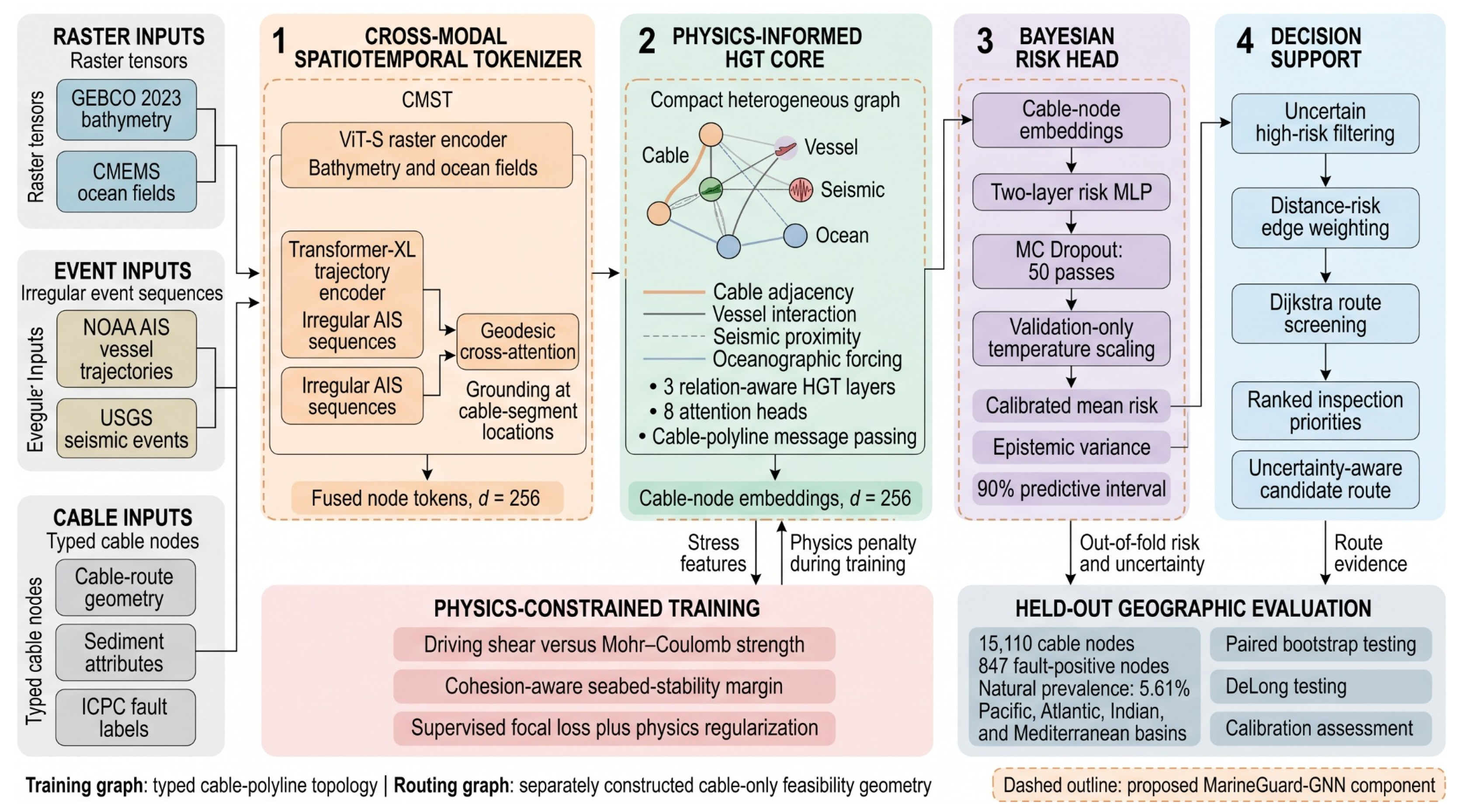
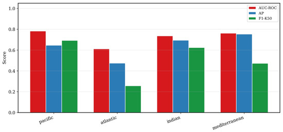
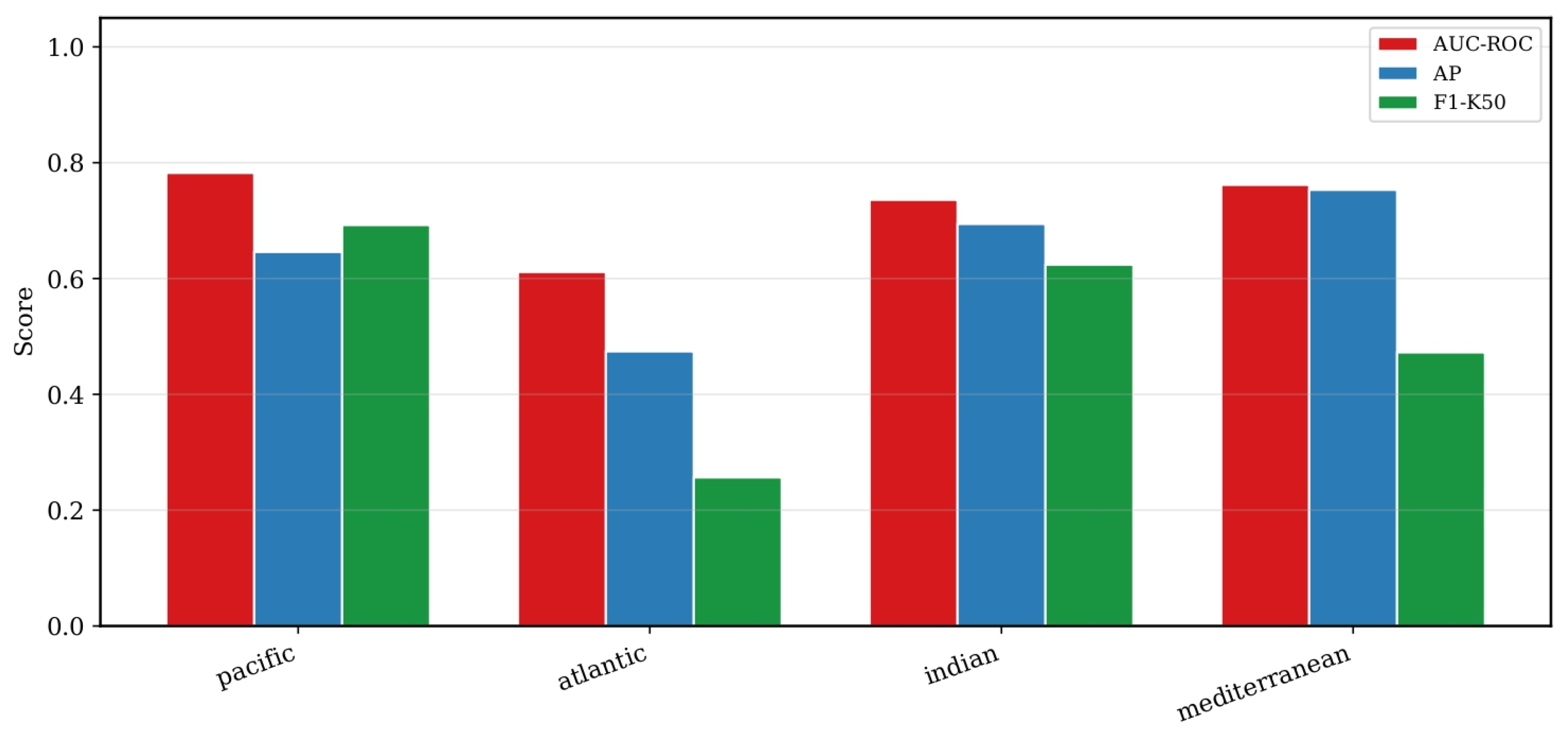
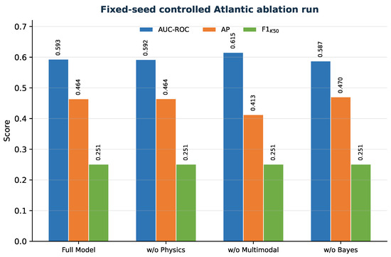
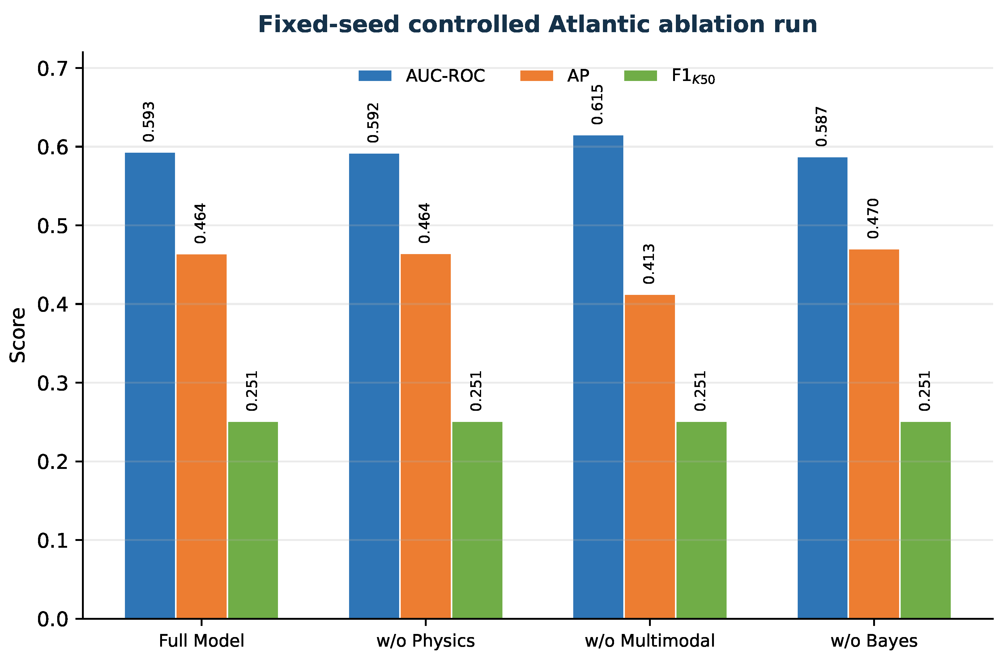
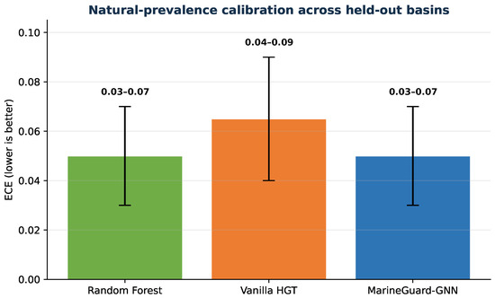
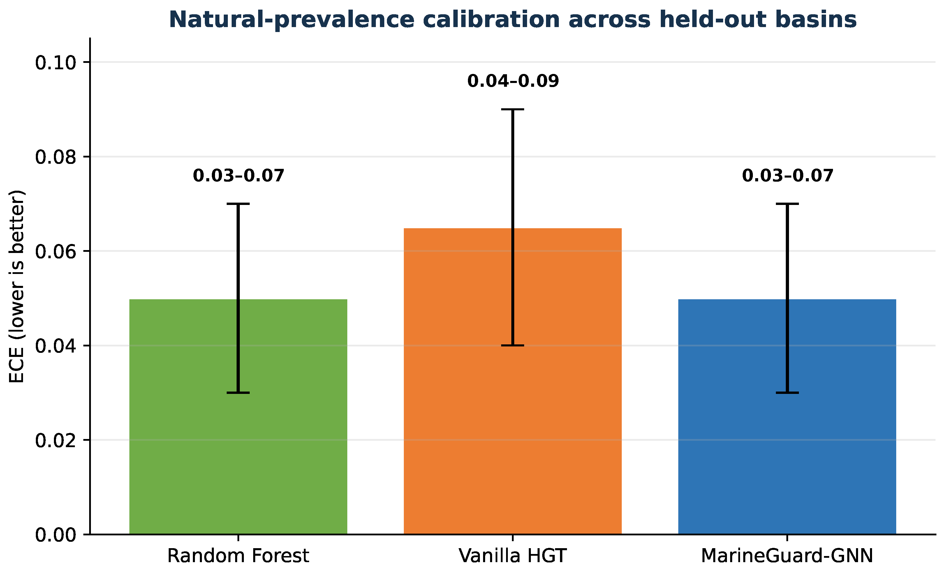
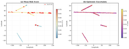
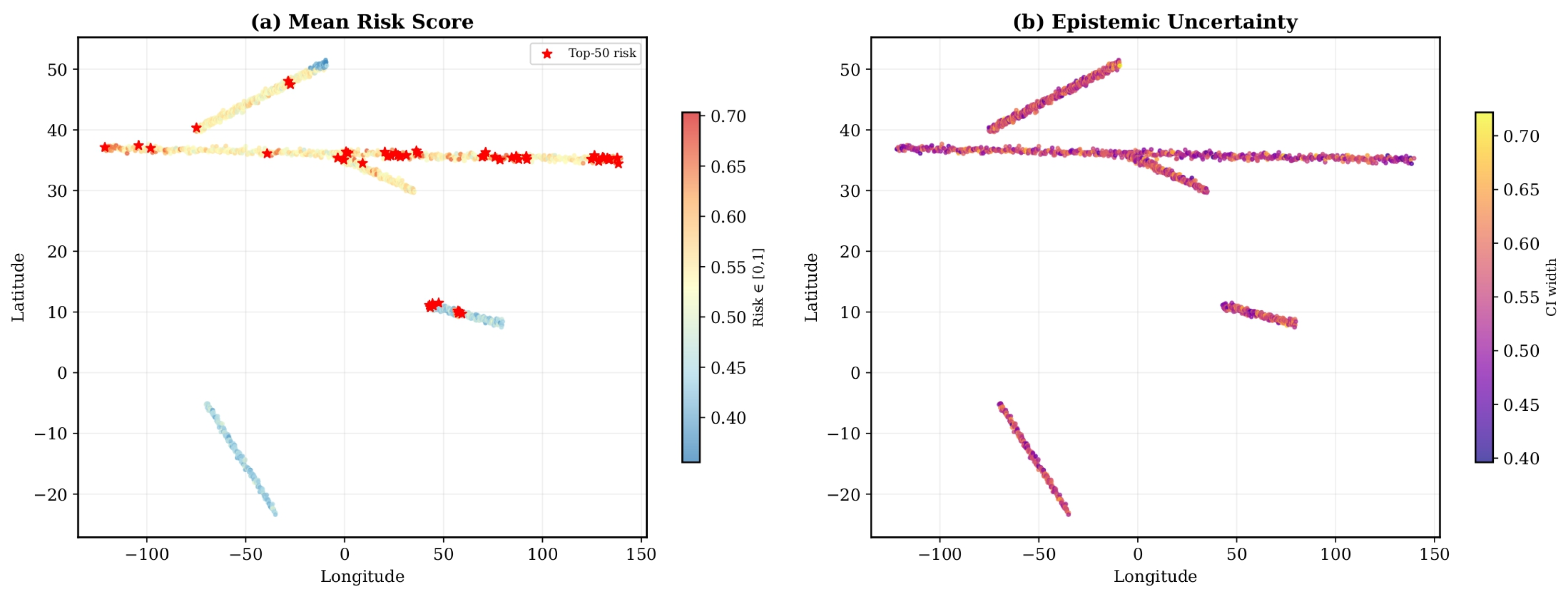
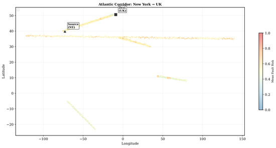
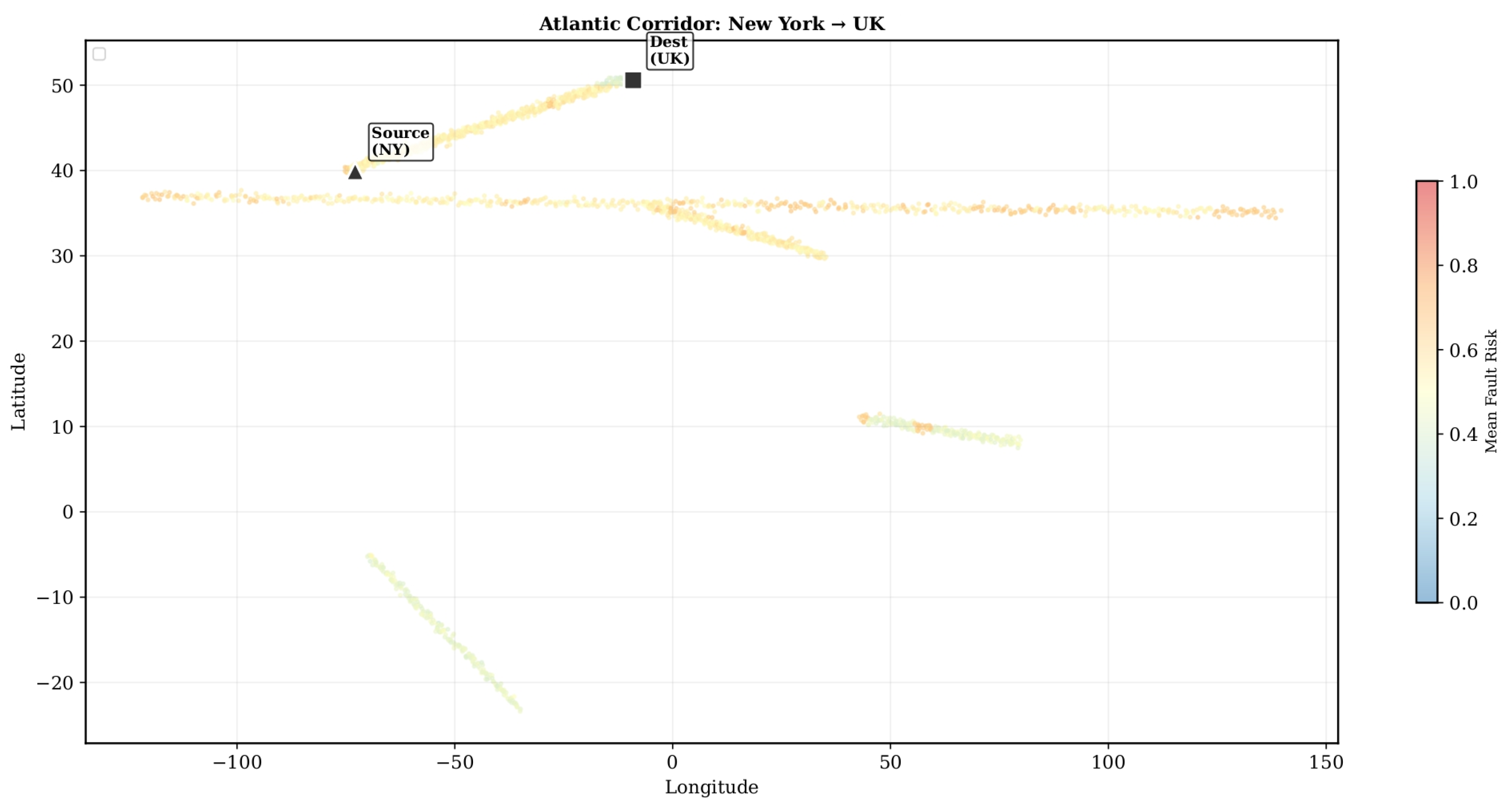
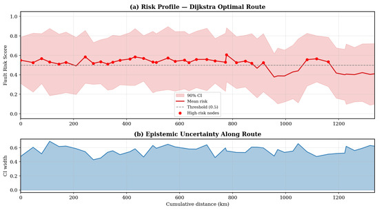
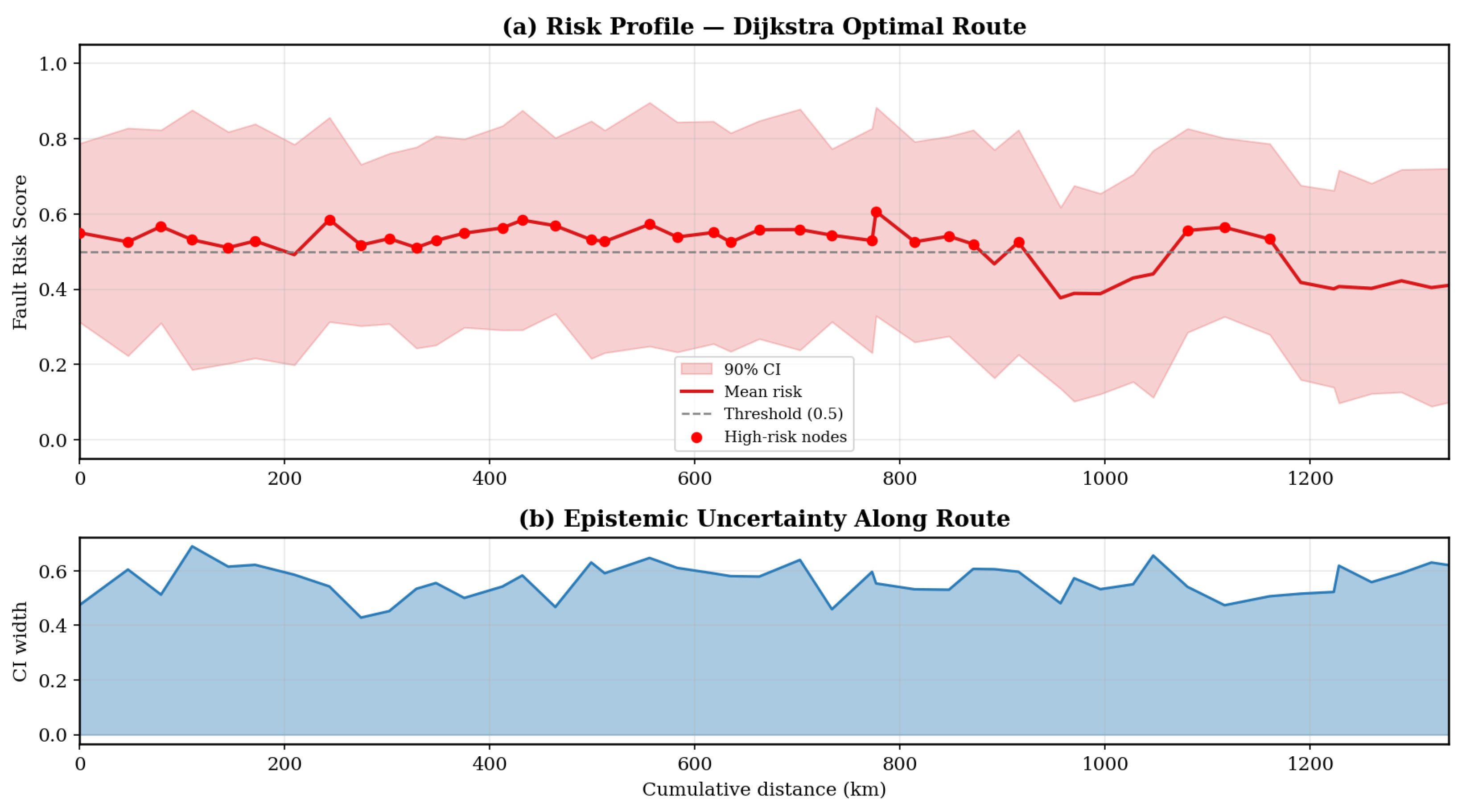

Disclaimer/Publisher’s Note: The statements, opinions and data contained in all publications are solely those of the individual author(s) and contributor(s) and not of MDPI and/or the editor(s). MDPI and/or the editor(s) disclaim responsibility for any injury to people or property resulting from any ideas, methods, instructions or products referred to in the content. |
© 2026 by the authors. Licensee MDPI, Basel, Switzerland. This article is an open access article distributed under the terms and conditions of the Creative Commons Attribution (CC BY) license.