


Abstract
Inland-vessel speed reductions targeted at priority segments can reallocate a normalized burden proxy across a fixed corridor. We develop a route-integrity speed-planning model that accepts a plan only when it attains the priority target, preserves route-wide improvement, and caps the largest non-priority-segment increase. The kinematics distinguish speed over ground, along-route current, and speed through water; without voyage-matched current or speed-through-water observations, the cases use zero-current analytical references. We evaluate two AIS-derived cases: the 27-point Case A as a sparse stress test and Case B as the primary spatial case after WGS84 and ESA WorldCover alignment checks. Under the equal-time constraint, an unprotected 2% target induces local deterioration. With a 0.5% non-priority cap, Case B supports a certified maximum target of 0.999%; a 2% late-arrival allowance raises the certified maximum target to 11.912%. Direct search over 0.1-kn commands finds a feasible plan for Case B; however, none of 1000 sampled ±0.2-kn execution-error profiles remains feasible. The framework identifies model-internal proxy transfer rather than measured energy, emissions, or exposure effects.
1. Introduction
Vessel speed jointly determines propulsion demand, transit time, and schedule reliability, making it a central operational decision in maritime transport [1,2,3]. On a fixed inland corridor, a local speed reduction cannot be evaluated in isolation. Slowing in a priority reach consumes schedule slack, delays arrival, or requires compensating speed changes elsewhere. A route-wide metric may therefore improve while another segment deteriorates. This interdependence creates a spatial acceptance problem that aggregate objectives can conceal.
Spatially differentiated management is already used in environmental and navigation practice, although the governing indicator differs by application. The Yangtze River Protection Law identifies protected drinking-water sources and important aquatic habitats as geographically explicit conservation priorities [4]. The Port of Los Angeles defines 20- and 40-nautical-mile vessel-speed-reduction zones for approaching and departing ships [5]. AIS-based studies also document spatially uneven ship activity and modeled emissions in the Yangtze River estuary, the middle Yangtze, and Tianjin [6,7,8], as well as in broader inland-waterway and port settings [9,10]. These examples illustrate how an authority or operator could designate route segments before optimization; they do not classify either AIS-derived case used here.
We refer to these preselected cells as priority segments. For a route with S segments, the computational experiment ranks the frozen exogenous weights from highest to lowest and selects approximately the highest-weighted 30%, with stable route order used to break ties; Section 4.2 gives the formal definition. The 30% share is a scenario defined by segment count, not a universal environmental or regulatory threshold. A field application could instead derive external weights from validated shoreline exposure, drinking-water or habitat protection, port activity, or published regulatory classes. In every case, the indicator, data source, spatial unit, threshold, tie rule, and update cycle must be declared before optimization begins.
Existing speed-planning models can optimize fuel, schedule, route choice, or environmental metrics, but they rarely ask whether a local target remains acceptable after schedule compensation is assigned along the rest of a fixed route. Aggregate objectives do not separately test local attainment, retained route-wide improvement, and the worst deterioration outside the target set. We use route integrity to name this joint acceptance problem. Its three conditions prevent a favorable route total from concealing the segment that absorbs compensation. These considerations motivate four research questions:
- •
- RQ1. Can an equal-time plan attain a priority target by transferring the normalized proxy to non-priority segments?
- •
- RQ2. How does a separate cap on every non-priority segment change feasibility and retained route-wide improvement?
- •
- RQ3. How do arrival slack, speed floors, physical-response assumptions, and trajectory representation change the supportable target?
- •
- RQ4. Does a continuous solution remain meaningful under finite command resolution and execution error?
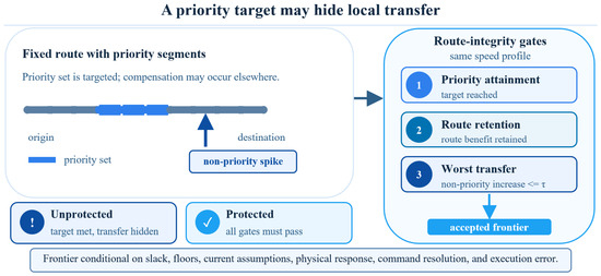
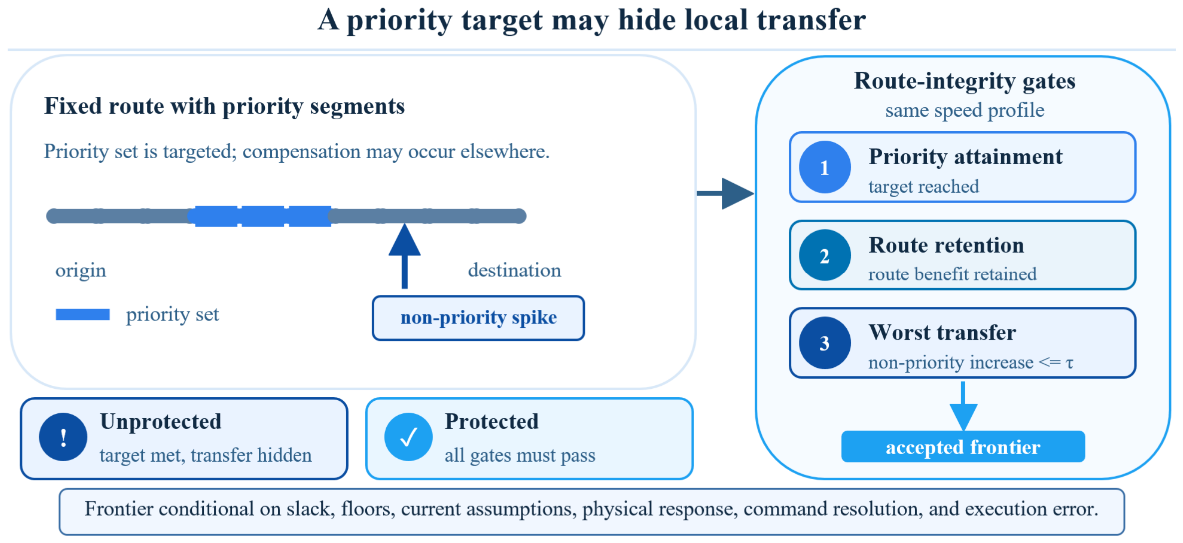
To answer these questions, we formulate a nonlinear segment-speed model referenced to an equal-time uniform benchmark (Figure 1). The protected formulation reports priority attainment, retained route-wide improvement, and the largest non-priority increase separately, and constrains every non-priority segment directly. We derive a feasibility-conditional retained-benefit bound and a speed-floor ceiling. For the zero-current pure-power reference, we construct a convex relaxation in reciprocal speed and obtain a matching dual bound, thereby certifying the principal-protected frontiers globally. The numerical study evaluates two AIS-derived computational cases across partitions, priority shares, arrival allowances, physical-response assumptions, command resolution, and execution error. The contribution is a route-integrity acceptance framework for fixed-path speed advice: it couples an ex ante spatial target with local non-priority protection and an explicit evidence hierarchy, distinct from propulsion-law development or generic solver design.
Figure 1.
Route-integrity acceptance logic for fixed-route speed planning. A priority-set target can be met while a non-priority segment absorbs a local increase; the protected formulation accepts a speed profile only when priority attainment, route-wide improvement, and the worst-local-transfer tolerance are all satisfied. The feasible frontier depends on arrival slack, speed floors, current assumptions, physical-response settings, command resolution, and execution error.
The remainder of the paper proceeds as follows. Section 2 reviews vessel speed planning, AIS-based spatial assessment, burden redistribution, trajectory representation, and operational decision support. Section 3 defines the problem setting, AIS-derived cases, trajectory partitions, and admissible speed domains. Section 4 formulates the load proxy, reference profiles, route-integrity models, and analytical properties. Section 5 describes the solution methods, experiment design, and numerical audit. Section 6 presents the numerical experiments. Section 7 discusses the main findings, conditional numerical results, operational implications, and limitations. Section 8 concludes.
2. Literature Review
Route-integrity speed planning draws on four research streams that are usually examined separately: maritime and inland-vessel speed optimization, AIS-based spatial assessment, location-specific transport impacts, and trajectory-based decision support. Their intersection matters because a segment-level intervention may be operationally feasible and spatially resolved yet fail to preserve its intended benefit after schedule compensation.
2.1. Vessel Speed Planning Under Route and Schedule Constraints
Maritime speed optimization formalizes the nonlinear relationship among speed, propulsion demand, voyage time, and service cost. Psaraftis and Kontovas [1,2] synthesize the principal speed models and their routing extensions, while Corbett et al. [3] quantify the economic and environmental consequences of slower service. Norlund and Gribkovskaia [11] show how operators can use schedule slack in supply-vessel planning. Later models integrate speed with bunker management, route choice, and emission-control policies [12,13]. This literature establishes that speed must be selected jointly with the service plan, but it usually evaluates environmental performance at the voyage, route, or network level.
Inland navigation localizes this coupling. Buchem et al. [14] optimize velocity under uncertain lock waiting and a traversal deadline, while Shao et al. [15] combine deployment decisions with non-identical streamflow and section-specific limits. Yan et al. [16] partition a route by environmental conditions, and Xu et al. [17] use rolling calculations for course and speed decisions in a traffic-separation waterway. Slagter et al. [18] compare leg-based plans for alternative propulsion systems under arrival constraints. These dynamic-environment and lock/schedule studies justify segment-level decisions, but they do not separately audit priority attainment, route-wide improvement, and the maximum deterioration in every non-priority segment.
Speed management is one component of maritime decarbonization and must remain consistent with route-specific technical and service constraints [19]. An aggregate indicator may decline even when the model shifts its weighted burden to another part of the corridor. The relevant question is therefore not whether speed affects energy use, but how a decision maker should accept or reject a local target when compensation elsewhere is unavoidable.
2.2. AIS-Based Spatial Assessment and Metric Boundaries
AIS data preserve the location, time, and speed information needed to move from voyage totals to spatially differentiated assessment. High-resolution inventories have been developed for the Yangtze River estuary, inland vessels, and the middle Yangtze [6,7,20]. Related studies localize ship activity and modeled emissions in ports and along inland waterways [8,9]. This research demonstrates why spatial position should be retained rather than collapsing all consequences into one voyage total. It also supplies the empirical basis for partitioning a traversal into decision segments and associating speed-dependent activity with each segment.
Spatial resolution alone does not establish physical or environmental validity. Comparisons between AIS-based estimates and onboard or localized measurements show that engine-load construction, low-load corrections, machinery characteristics, and emission factors can materially change absolute results [8,9,20]. Translating vessel activity into ambient concentration requires dispersion or atmospheric-chemistry modeling, while estimating health burden further requires population data and concentration-response functions [7,21]. These analytical layers answer different questions and should not be compressed into a single generic environmental metric.
Accordingly, we use the normalized segment-weighted load proxy for within-case comparisons under a fixed assumption set. The proxy reveals whether optimization reallocates the modeled weighted burden across route segments; subsequent interpretations refer to this proxy rather than to fuel consumption, emitted mass, air quality, exposure, health damage, or carbon reduction.
2.3. Spatial Redistribution and Local Safeguards
Freight-routing research provides the most explicit treatment of spatially uneven transport impacts. Luo et al. [22] combine truck routing with emissions, dispersion, and population information to reduce community-wide exposure under a travel-time limit. Dennis-Bauer et al. [23] incorporate human exposure and health costs into freight traffic assignment. Both studies show that a system-wide improvement does not guarantee a benefit at every affected location and that local safeguards can change the preferred transport plan.
Observed vessel-speed-reduction programs provide a maritime counterpart. Woo and Im [10], for example, use AIS observations to evaluate a port speed-reduction program under realized operating patterns. Such studies are valuable for assessing port-scale or aggregate outcomes, but they do not formulate the compensation mechanism of a vessel that slows in selected route sections while maintaining a fixed path and an arrival requirement.
A fixed inland route changes how redistribution occurs. Road freight can redirect vehicles among alternative paths, whereas an inland vessel usually has little path-choice flexibility within a prescribed corridor. Redistribution therefore operates through segment speed and residence time. A route-wide non-worsening constraint can control the aggregate result but cannot rule out a large increase in one non-priority segment. Conversely, a priority-set constraint can certify nominal attainment while leaving little of the priority-set contribution in the route total. We therefore distinguish three acceptance quantities: reduction inside the priority set, route-wide improvement retained after compensation, and the largest increase outside the priority set.
2.4. Trajectory Representation and Operational Decision Support
A speed recommendation operates within an established navigation and traffic-management system. IMO and IALA guidance retain navigational authority with the vessel master and position VTS tools as decision support rather than autonomous control [24,25,26]. Applicable navigation rules provide the broader safety framework [27]. A useful optimization result should therefore disclose the arrival margin, binding local constraints, and sensitivity to uncertain conditions, while safety, traffic, visibility, under-keel clearance, and machinery limits remain controlling considerations.
The screening model must also state its physical scope. Maritime models and inventory guidance commonly relate speed to propulsion load through a power law [28,29]. The resulting estimates nevertheless depend on vessel characteristics, operating mode, current, auxiliary demand, and low-load behavior. A normalized power-law proxy can support mechanism analysis and analytical bounds, but absolute energy or emission claims require vessel-specific calibration.
Trajectory preprocessing defines the units on which the local constraints operate. AIS simplification removes redundant observations, whereas segmentation determines where one operating regime ends and the next begins. Zhang et al. [30] formalize trajectory simplification and threshold selection. Ye et al. [31] develop behavior-based adaptive segmentation, and Balcer et al. [32] show that trajectory simplification can change modeled ship carbon emissions. A segment-level optimization may therefore remain numerically stable under one partition while referring to different physical intervals under another.
Decision-support studies have examined vessel speed advice under uncertain operating information and service commitments [33]. Existing work, however, does not combine local protection, schedule slack, trajectory partitioning, command quantization, and execution error within a fixed-route targeting framework. These implementation features determine whether a continuous frontier is only mathematically feasible or can support an auditable advisory profile.
The closest formulations differ in decision unit, target timing, and acceptance rule. Maritime models optimize voyage or network aggregates; inland studies address either dynamic environmental speed decisions or lock, schedule, and propulsion planning; exposure-aware studies change paths; and port programs evaluate predefined zones. The reviewed studies do not jointly combine an ex ante priority set on a fixed path with separate tests for local attainment, retained route-wide improvement, and the worst non-priority increase. Table 1 makes this formulation-level contrast explicit.
Table 1.
Closest-formulation comparison and the route-integrity gap.
We address this gap with an acceptance rule rather than a new generic optimizer. Its first layer verifies attainment within the priority set, its second measures the improvement retained over the full route, and its third limits deterioration in every non-priority segment. The analytical bounds follow from the accounting definitions and speed domain. Numerical and convex-dual audits then determine whether the full constraint set can be satisfied for a specified schedule, partition, and response model.
3. Problem Description
3.1. Problem Setting and AIS-Derived Cases
We analyze two single-voyage, AIS-derived computational cases supplied by a third-party provider. The supplied AIS files contain timestamp, longitude, latitude, course over ground (COG), speed over ground (SOG), and heading; they contain no current vector or speed-through-water field, consistent with the standard AIS dynamic-message scope [36]. Case A has 27 cleaned observations over 3.666 h on 12 January 2025 and covers 24.128 nautical miles. Case B has 853 observations from 00:25:08 to 03:19:55 on 14 November 2025, covers 18.641 nautical miles, and has strictly increasing timestamps. Median sampling intervals are 595.5 s and 8 s; maximum intervals are 614 s and 159 s.
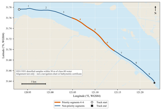
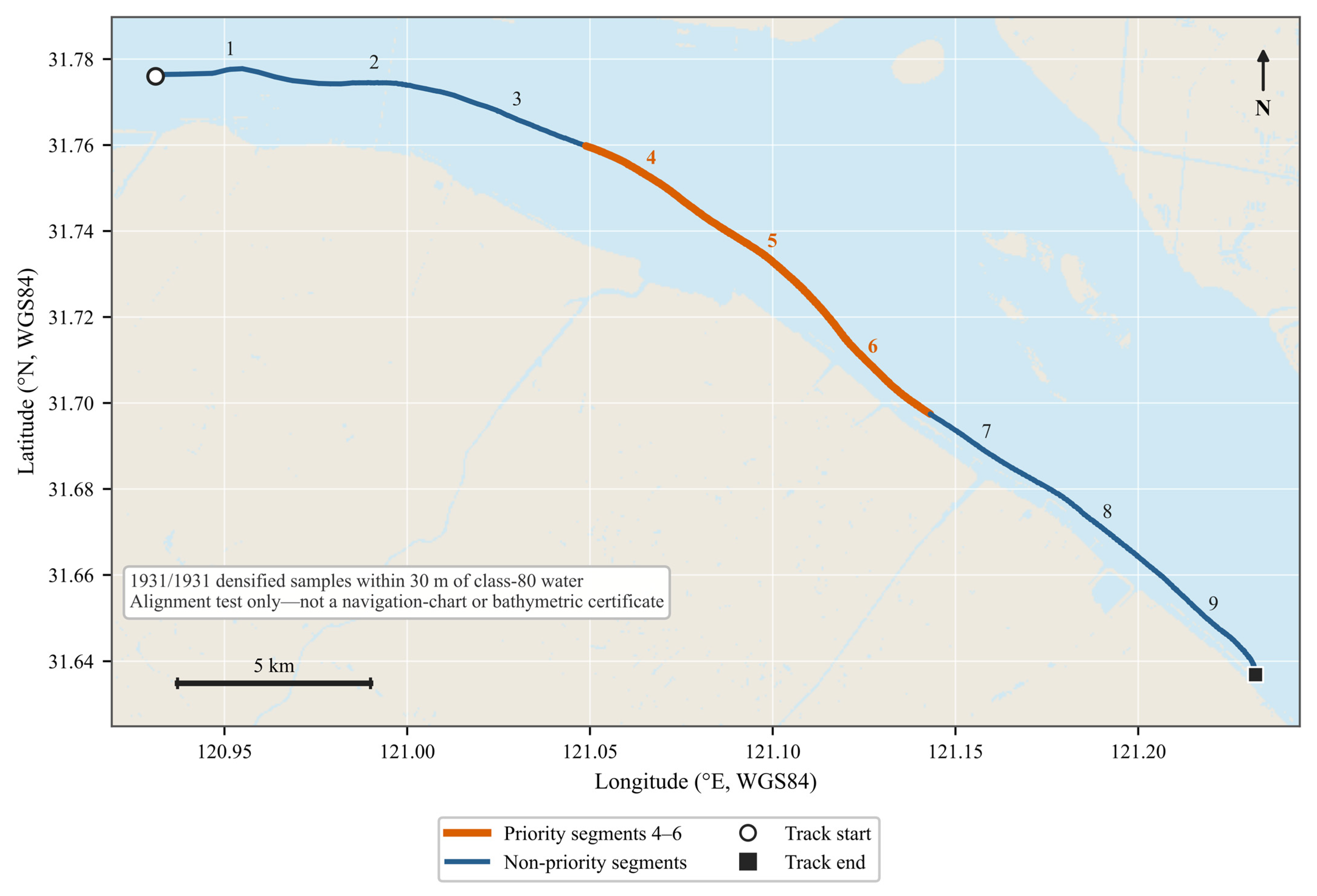
We treat Case A as a sparse-data stress test suitable only for route-scale redistribution analysis; it cannot resolve acceleration, engine transients, or real-time control. Case B receives a separate geospatial audit. The provider dictionary declares WGS84, and the source DMS labels reproduce the exported decimal coordinates to within 3.4 × 10⁻⁹ degrees. We densified the 18.641 nm track to 1931 points at no more than 25 m spacing and tested each point against ESA WorldCover 2021 class-80 water within 30 m [37]. The declared WGS84 branch passed for 1931/1931 samples with no non-water run (Figure 2). Diagnostic GCJ-02 and BD-09 inverse transformations were not used to select the coordinate system; the BD-09 branch failed the predeclared alignment rule. This verifies coordinate and land-cover alignment for Case B, not navigational clearance, bathymetry, or current.
Figure 2.
Case B WGS84 track and route-water alignment. Priority segments 4–6 are orange. All 1931 points densified at ≤25 m spacing lie within 30 m of ESA WorldCover 2021 class-80 water. This is a land-cover alignment test, not a navigation chart or bathymetric certificate. © ESA WorldCover project 2021/contains modified Copernicus Sentinel data (2021) processed by ESA WorldCover consortium [37].
Table 2 reports the cases and settings; positive percentage changes denote improvement relative to the equal-time uniform profile. Source-to-normalized row checks reproduced all six supplied fields for both voyages. The supplied AIS exports, legacy files, and associated weather-panel sample do not contain voyage-matched stream speed, stream direction, or speed-through-water series; SOG is therefore retained as speed over ground rather than converted to speed through water. A provider field lists 1202 kW and two main engines for Case A, but the engine model, rated speed, auxiliary demand, fuel type, and primary technical source are not provided. We therefore exclude that field and do not compute absolute power, fuel, emissions, carbon, exposure, health, or monetary cost.
Table 2.
AIS-derived cases and principal experimental settings.
3.2. Trajectory Segmentation and Admissible Speed Domain
We reconstruct each case under four route partitions. The baseline contains 12 equal-distance segments for Case A and nine for Case B; the coarse and fine alternatives contain six and 18 equal-distance segments in each case. A dynamic-programming change-point procedure minimizes within-segment speed variance subject to minimum cell counts and produces eight segments for Case A and 12 for Case B. For each partition, we recompute segment distances, travel times, weights, bounds, priority-set membership, and all optimization constraints.
A segment’s support count records the number of contributing trajectory intervals; an interval that crosses a boundary may contribute to more than one segment. Across the Case A coarse, baseline, fine, and change-point partitions, the minimum/median/maximum support counts are 4/5/7, 1/2/4, 2/2/4, and 1/4/9. The corresponding Case B minima range from 6 to 30. The protected baseline Case A result comes from the sparsest representation and should not be interpreted as partition-robust empirical evidence.
We retain computational domains of 6.5–12 kn for Case A and 6–12 kn for Case B as frozen numerical scenario definitions. The lower bounds are 0.081 and 0.399 kn below the respective equal-time uniform benchmarks of 6.581 and 6.399 kn. They were not derived from vessel-specific operating limits; therefore, all maximum-target results are conditional on these settings, and cross-case differences partly reflect unequal deceleration slack. The common 12 kn upper bound equals the reference speed; at that bound the pure-power reference load is 0.75, below the 0.85 screening ceiling. Adjacent commands may differ by at most 1 kn as an uncalibrated numerical regularity rule; the largest realized change among certified cells is 0.409 kn. Table A4 reports the speed-floor sensitivity, and Table A6 records the adopted domains and transition rule. None of these settings is presented as a statutory, vessel-specific, acceleration, actuator, maneuvering, or safety limit.
The kinematic distinction is central to the evidence boundary. In the model, SOG determines residence time, whereas speed through water drives the propulsion response after accounting for the along-route current component. The voyage files do not contain synchronized current vectors or speed-through-water observations, so the reported main cells use cs = 0 as a zero-current analytical reference, not as an observed calm-water condition. Nonzero-current cases are synthetic sensitivity fields. A field application would require synchronized current and speed-through-water data, current-aware bounds, and route-specific validation [15,16].
4. Model Formulation
4.1. Segment-Level Load Proxy
Let S denote the segment set. For segment s, let ds be the distance, vs speed over ground, and ts be the travel time. For current-aware kinematics, let cs be the signed along-route current component (positive with the route) and us = vs− cs be the speed through water. Travel time follows
The current-aware normalized propulsion response is evaluated at speed through water:
Multiplying the current-aware propulsion load by residence time gives the normalized propulsion load-hour contribution:
Equations (2) and (3) separate propulsion, which is evaluated through speed through water us, from residence time, which depends on speed over ground vs. Equation (2) uses Lref = 0.75, vref = 12 kn, and the screening exponent γ = 3. Because cs and us are not observed in the voyage files, the main cells set cs = 0, so us = vs and Equations (2) and (3) reduce to the zero-current analytical reference used in the optimization and certificates. The scale constants support within-case percentage comparisons; they are not estimates of service speed, design speed, or maximum continuous rating. Cubic speed-load behavior is a common screening approximation [1,2], but measured emissions and low-load behavior can be non-monotone and pollutant-specific [20,35]. We vary γ to reflect this uncertainty and keep the proxy distinct from measured fuel or emissions.
To represent non-propulsive demand, we add a constant auxiliary or hotel-load share q relative to the reference propulsion scale. Here q is auxiliary load divided by the reference propulsion load Lref; it is not the fraction of total instantaneous load. The resulting Es and Ps are normalized load-hours (unit h) before conversion into within-case ratios:
Under the cs = 0 specialization used in the main experiments, the propulsion term varies with vsγ−1, whereas the auxiliary term varies with 1/vs. The stationary point of the combined expression is
When the feasible speed interval lies above vs*, reducing speed lowers the combined proxy, but less strongly than under the pure-power specification. If the interval crosses vs*, additional slowing can increase the combined term. We therefore treat q = 0.10 and q = 0.20 as conditional physical scenarios rather than vessel-specific estimates.
Assign each segment an exogenous priority weight ws and normalize the weights to a route mean of one. The segment-level weighted load-hour proxy is
Equations (2) and (3) make the nonzero-current distinction explicit: propulsion depends on us = vs − cs, while residence time depends on vs. The auxiliary component in Equation (4) grows with residence time. In the empirical main cells, cs = 0 and the two speeds coincide. Es and Ps retain time units before route-normalized percentage comparisons are formed. These definitions make the proxy suitable for within-case comparisons under fixed assumptions, not for conversion into fuel, emissions, exposure, health, or carbon estimates.
For the two frozen baseline cases, ws comes from the normalized scenario-input file rather than an external receptor dataset. It is assigned piecewise by route group and normalized to an arithmetic segment mean of one. Case A uses 3.008 for segments 1–3, 0.172 for 4–6, 0.161 for 7–9, and 0.658 for 10–12; Case B uses 1.029 for 1–3, 1.177 for 4–6, and 0.794 for 7–9. Table A5 reports the complete mapping. These values rank a diagnostic scenario; they do not represent shoreline, population, ecological, concentration, exposure, or health evidence.
4.2. Reference Profiles and Priority-Segment Selection
The observed AIS speed vector is descriptive and may violate the computational speed bounds or the adjacent-speed rule. We therefore project it onto the admissible domain by minimizing squared deviation from the observed segment speeds while preserving total travel time. This projected vector defines the schedule-feasible reference. The corresponding equal-time uniform benchmark is
The uniform profile isolates the targeting mechanism from the generic smoothing benefit of an irregular speed vector. The observed vector summarizes the provider export, the projected vector establishes an admissible schedule, and the uniform vector supplies the common benchmark for spatial targeting.
The primary priority set follows the predeclared rule in Section 1. For S segments, we select K = max(1, ceil(0.30S)) after sorting frozen exogenous weights in descending order; stable route order breaks ties. The 30% share is a scenario by segment count, not a universal threshold. In an application, an authority must first select the indicator and source, fix the spatial partition, transform the indicator to segment weights, and freeze the share, threshold, tie rule, and update cycle before optimization. We recompute membership only when an explicitly defined partition or weight scenario changes.
For sensitivity analysis, we also define a controllability-oriented priority set. Its ranking score is
The score identifies segments in which the speed decision has leverage relative to the assumed floor. We do not use it as the primary policy definition because it depends on the modeled speed domain. To compare priority sets across partitions, we divide their shared along-route distance by the union of the two interval sets. This distance-weighted overlap avoids comparing segment identifiers that refer to different partitions.
4.3. Route-Integrity Optimization Models
Let denote the fixed priority set and its complement. Let the symbols in Equations (11) and (12) denote the priority-set and route totals under the uniform benchmark. For a prescribed priority target and non-priority tolerance , the equal-time model minimizes normalized energy plus a small smoothness penalty:
We impose equal route travel time through
The priority-set target requires
We prevent aggregate route deterioration with
We impose route integrity by constraining each non-priority segment separately:
The speed domain, adjacent-speed transition rule, and normalized-load limit complete the feasible set:
The experiments use a 1 kn adjacent-speed limit, a normalized-load upper bound of 0.85, and a smoothness coefficient of 0.001 kn−2. Because the squared adjacent-speed difference in Equation (9) has units of kn2, the coefficient carries kn−2; the penalty is therefore dimensionless. It is a numerical tie-breaker, not a physical parameter. The sensitivity grid at 0, 10−4, 10−3, and 10−2 kn−2 covered three named baseline cells: Case A with ρ = 2%, τ = 0.5%, η = 0; Case B with ρ = 2%, no non-priority cap, η = 0; and Case B with ρ = 0.9%, τ = 0.5%, η = 0. Feasibility and the priority target were preserved in all three. Route-wide improvement varied by at most 1.5 × 10⁻⁴ percentage points, while local allocation changed more, so every profile is recalculated and constraint-audited independently of the objective.
To allow schedule flexibility, we replace exact time equality with a no-early-arrival condition and a maximum late-arrival allowance η:
For each η, the frontier model minimizes the priority-set ratio subject to the route cap, the selected non-priority tolerance, and all remaining feasibility constraints:
For selected priority targets, a second model identifies the smallest audited delay among the multistart solutions:
Because SLSQP is a local nonlinear solver, ‘smallest audited delay’ means the lowest delay among independently verified multistart solutions; it does not certify the global minimum.
4.4. Analytical Properties
Let denote the share of the total uniform-benchmark route contributed by the priority set:
Define retained route-wide improvement as
Proposition 1 (retained-benefit bound): If a feasible profile attains the priority target and every non-priority segment satisfies tolerance , then
Equation (20) follows by applying Equation (11) to the priority-set contribution and Equation (13) to every non-priority contribution. Summing the two parts, dividing by the uniform-benchmark route total, and subtracting the ratio from one gives the bound. The derivation uses only the common accounting definitions and requires neither convexity nor a particular solver.
A strictly positive retained route improvement is guaranteed whenever
For , define the fraction of the nominal priority-set contribution offset outside the priority set as
An offset ratio of 100% means that changes outside the priority set fully erase its nominal contribution to route-wide improvement. The bound remains conditional on feasibility: it characterizes every feasible cap-constrained profile but cannot make an infeasible target attainable.
Proposition 2 (speed-floor ceiling): Under the pure power-law response, with no auxiliary term or current correction, define the floor ratio as the priority-set-weighted mean of each segment’s floor-to-uniform-speed ratio raised to . Use weights proportional to segment distance and priority weight. The speed domain then implies
If all priority segments share one speed floor, Equation (23) reduces to the common-floor expression. The ceiling is an upper bound rather than a feasibility guarantee because arrival, transition, route, or non-priority constraints may bind first. Auxiliary demand and current corrections change the functional form and lie outside the proposition. The nesting of feasible sets also implies two monotonicity results: increasing cannot reduce the frontier, whereas tightening cannot increase it.
5. Solution Methods and Verification
5.1. Multistart Optimization and Independent Feasibility Audit
We solved continuous problems with SLSQP from the uniform benchmark, projected reference, five targeted priority reductions, and seeded Gaussian perturbations (seed 20260716). Baseline problems used six to eight random starts in addition to deterministic profiles; alternative partitions used three, and sensitivity cells used two to five. Each run allowed 1200 iterations with ftol = 10−10. All experiments were rerun under a frozen configuration, and accepted and rejected starts were retained.
We recalculated candidate profiles outside the optimizer before accepting them. The independent audit checked speed and arrival bounds, adjacent-speed differences, maximum normalized load, normalized energy where applicable, the route total, priority attainment, and every non-priority cap. A run was accepted only if every check met the general tolerance of 4 × 10⁻⁷ and the route-time tolerance of 3 × 10⁻⁵ h. The diagnostic record retains both accepted and rejected runs. The multistart optimization, independent feasibility audit, and certification workflow is summarized in Algorithm 1.
| Algorithm 1. Multistart optimization, independent feasibility audit, and certification workflow | |
| Step | Operation |
| 1 | Read the frozen case data and scenario parameters. |
| 2 | Construct deterministic and seeded initial speed profiles. |
| 3 | Solve the continuous model from every initial profile. |
| 4 | Recalculate the objective and all constraints outside the optimizer. |
| 5 | Reject any run that violates the numerical or route-time tolerances. |
| 6 | For eligible pure-power cells, solve the reciprocal-speed primal relaxation and Lagrangian dual. |
| 7 | Verify the target-interval gap and the omitted adjacent-speed rule. |
| 8 | Return the best audited profile and write the complete diagnostic record. |
5.2. Maximum-Target Global Certification for the Pure-Power Baseline
For the continuous pure-power baseline (γ = 3, zero current, q = 0), we certify the maximum priority target for a fixed priority set, non-priority protection rule, and arrival allowance. Setting xs = 1/vs makes route time affine and each segment proxy proportional to xs−2. Speed bounds and non-priority caps become box bounds, while the route constraint remains convex. We remove only the adjacent-speed-difference rule, solve the resulting convex relaxation, and evaluate a separable Lagrangian dual lower bound. If the relaxation optimizer also satisfies the removed rule and the primal objective meets a dual-feasible bound within tolerance, the resulting interval certifies the maximum target of the original continuous frontier problem. Appendix A provides the complete primal and dual formulations, strong-duality conditions, interval calculation, and numerical tests.
This certification is limited to the baseline maximum-target frontier. We apply it to 14 baseline cells: the six 30% priority-share cells with a 0.5% cap and arrival allowances of 0%, 1%, and 2%, together with the 20% and 40% share cells at 0% and 2% arrival allowances. A cell is labeled certified only after reciprocal-speed primal feasibility, verification of the original adjacent-speed rule, and a feasible-objective/dual lower-bound gap no larger than 2 × 10⁻⁷. Table 3 reports the cell-level maximum-target certificates. The largest realized target-interval gap is 3.4 × 10⁻¹³ percentage points, and the largest adjacent speed change is 0.4092 kn, below the original 1 kn limit. Current, auxiliary-load, alternative-partition, discrete-speed, and execution-error tests remain outside this certificate.
Table 3.
Maximum-target primal-dual certificates for the 14 continuous pure-power baseline cells (non-priority tolerance τ = 0.5%).
5.3. Scenario Matrix and Sensitivity Design
The experiment matrix contains four segmentations per case: priority shares of 20%, 30%, and 40%; arrival allowances of 0%, 1%, and 2%; and non-priority tolerances of no cap, 1%, 0.5%, and 0%. It also varies the speed exponent, speed floors, auxiliary shares, weights, and priority-set selection. Synthetic uniform and heterogeneous current fields replace voyage-matched current, which is not observed. Auxiliary shares q = 0.10 and 0.20 are diagnostic stress-test points relative to reference propulsion load rather than vessel measurements or calibrated operating ranges.
5.4. Discrete-Command Search and Execution-Error Stress Test
We search the discrete command space directly rather than rounding a continuous solution. Speeds are encoded in 0.1 kn units and searched by integer-coded differential evolution with 220 iterations, population 14, mutation [0.5, 1.0], recombination 0.7, one worker, and no SLSQP polishing. The test imposes a 2% target, 0.5% non-priority cap, and 1% late-arrival allowance. Failure to find a command is a negative search result, not an infeasibility proof. Execution errors are independently sampled by segment from U[−b, b], b ∈ {0.1, 0.2} kn, then clipped to bounds. We audit 1000 seeded draws before and after time-only rebalancing. The fractions describe this artificial sampler and are not reliability probabilities.
5.5. Reproducibility Package
All experiments were run in Python 3.12.13, NumPy 2.3.5, pandas 3.0.1, and SciPy 1.16.3 on Windows 11 with IEEE-754 binary64 arithmetic [38]. The archived reproducibility package records normalized inputs, parameter files, solver settings, versions, hashes, accepted and failed starts, stage runtimes, regularizer sensitivity, priority-share audits, and reciprocal-speed primal-dual certificates. Differential evolution supplies an independent search path for the discrete problem, separate from the certified continuous frontiers.
6. Numerical Experiments
6.1. Core Equal-Time and Arrival-Frontier Results
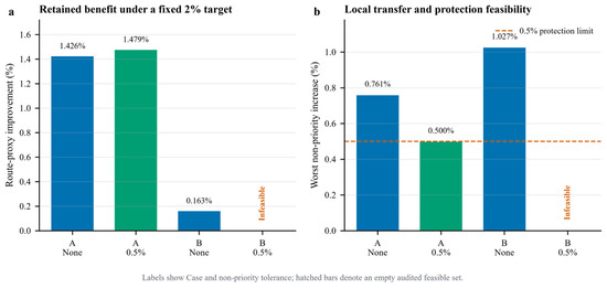
Both baseline cases attained the unprotected 2% target (Table 4 and Figure 3). Case A retained a 1.426% route improvement, offset 9.92% of the nominal priority contribution, and reached a 0.761% maximum non-priority increase. Case B retained only 0.163%, offset 79.13%, and reached 1.027%. Both exceeded the 0.5% diagnostic cap, and Case B transferred most of the nominal priority contribution.
Table 4.
Equal-time results for a 2% priority-segment target under the baseline priority sets.
Figure 3.
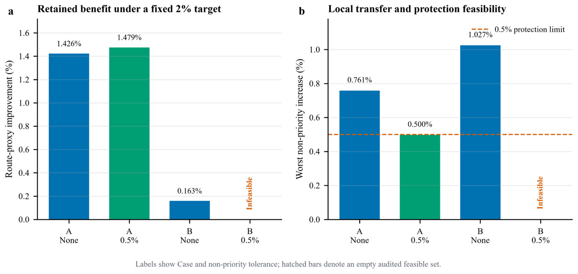
Equal-time mechanism for a 2% priority-segment target. Panel (a) reports retained route-wide improvement and panel (b) the largest non-priority increase; the dashed line is the 0.5% cap. ‘Infeasible’ means no audited solution satisfied the full stated constraint set.
With τ = 0.5%, the cases diverged. Case A retained a 1.479% route-wide improvement. The maximum non-priority increase reached the 0.5% cap, while the retained improvement equaled the analytical lower bound to the reported precision. This is the only protected 2% result found across eight representations, and its baseline segments have minimum and median support of one and two; we treat it as an illustrative sparse-data configuration. For baseline Case B, the certified maximum target is 0.999%, ruling out the protected 2% target under the equal-time constraint.
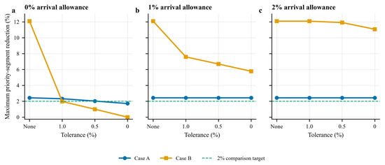
Arrival flexibility: Arrival flexibility changes the protected frontier (Table 5 and Figure 4). Under the equal-time constraint, tightening the cap from none to 0.5% reduced the maximum target from 2.439% to 2.029% in Case A and from 12.088% to 0.999% in Case B. The 0.5–cap values are globally certified for the continuous pure-power zero-current reference; uncapped and alternative-physics cells are audited numerical results.
Table 5.
Largest audited priority-segment target under alternative caps and late-arrival allowances; 0.5–cap baseline cells report globally certified maximum targets.
Figure 4.
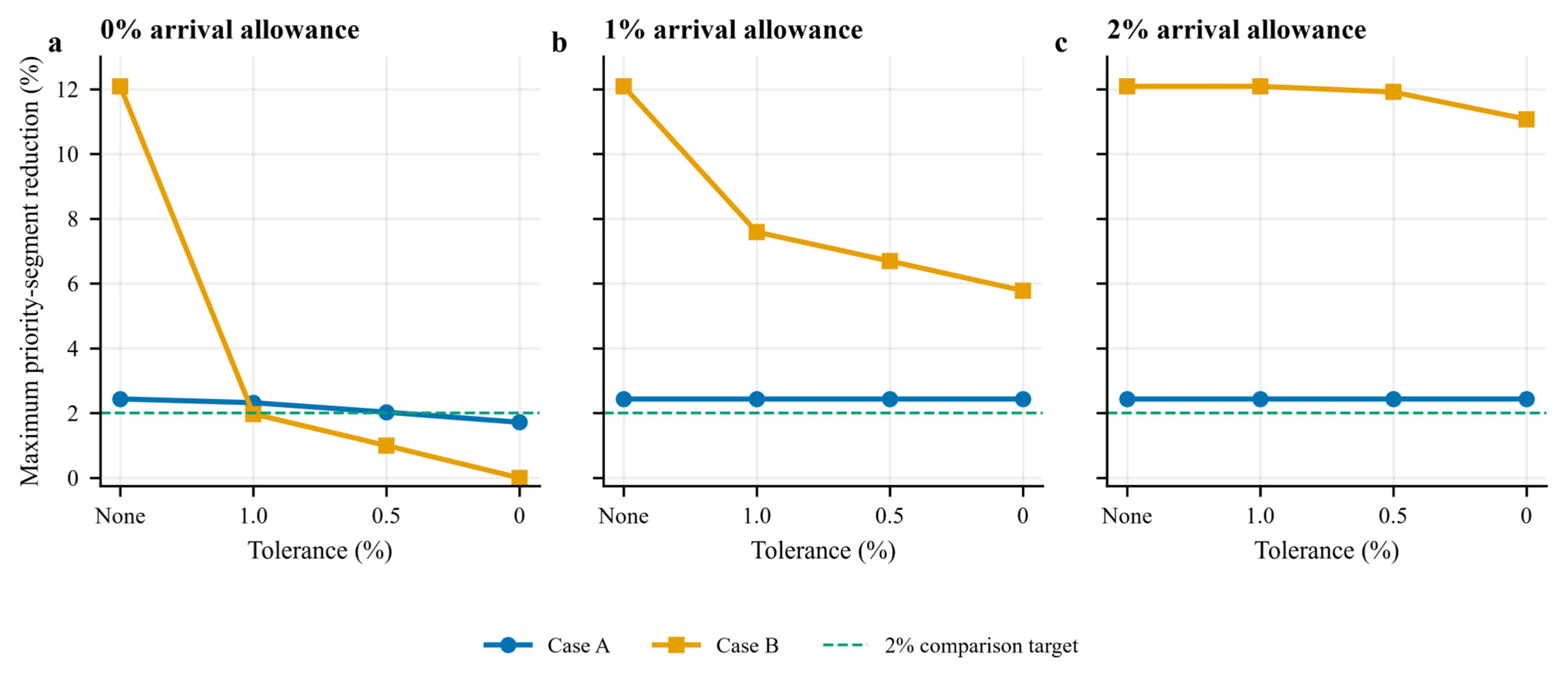
Protected maximum target under alternative non-priority caps and late-arrival allowances: (a) 0% late-arrival allowance; (b) 1% late-arrival allowance; (c) 2% late-arrival allowance. In all panels, the blue solid line with circular markers denotes Case A, the orange solid line with square markers denotes Case B, and the green horizontal dashed line marks the 2% comparison target. Only the 0.5%-cap pure-power zero-current baseline cells are globally certified.
With the 0.5% cap, a 1% late-arrival allowance produced certified maximum targets of 2.439% in Case A and 6.694% in Case B; a 2% late-arrival allowance produced 2.439% and 11.912%. Case A remained at its speed-floor ceiling. Because the frozen case definitions provide unequal deceleration slack, part of the cross-case response to additional time is attributable to those bounds rather than vessel-specific operating differences; Table A4 reports the speed-floor sensitivity.
The frontier therefore quantifies a schedule-protection trade-off in the normalized proxy. Because delay costs, absolute fuel consumption, and carbon prices are not observed, it should not be read as a monetary or carbon optimum.
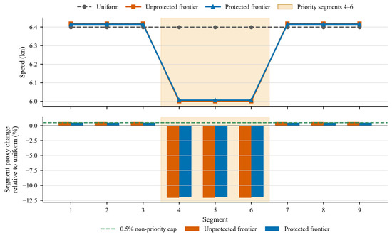
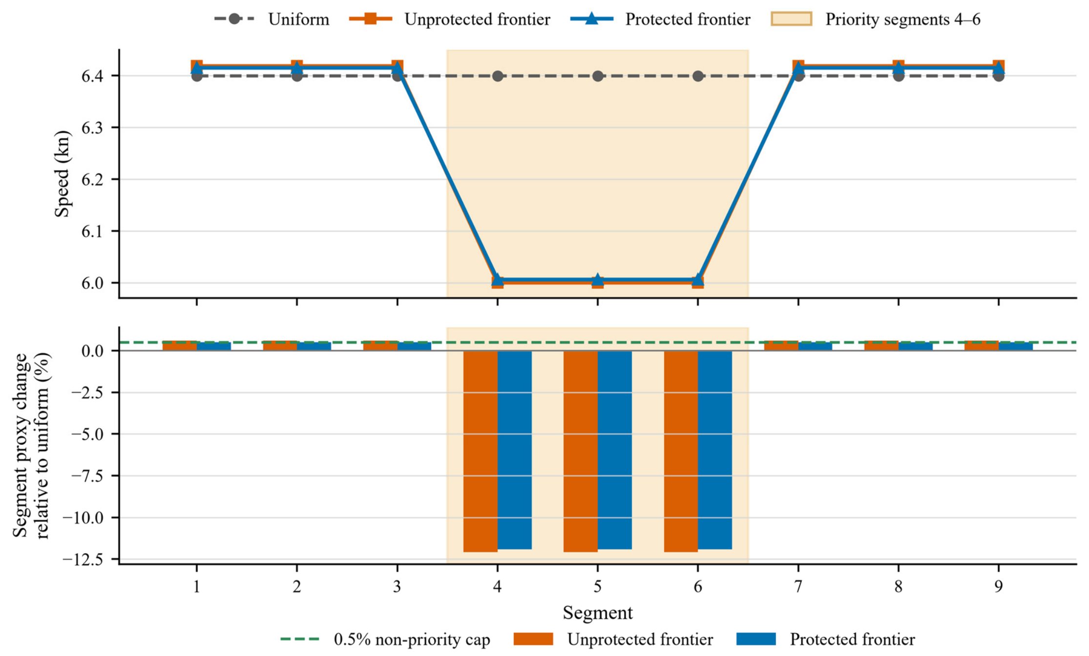
Figure 5 localizes the Case B mechanism under a common 2% late-arrival allowance. The unprotected frontier raises every non-priority segment above the uniform benchmark. The protected frontier holds those changes at the 0.5% cap and concentrates reductions in priority segments 4–6.
Figure 5.
Case B segment profiles for the 2% late-arrival frontier. The legend identifies the orange priority-zone shading for segments 4–6. The protected pure-power zero-current profile imposes τ = 0.5%; the lower-panel dashed line marks that cap. Its globally certified maximum target is 11.912%.
6.2. Representation and Physical-Response Sensitivity
Across the four partitions per case, the unprotected 2% target under the equal-time constraint remained feasible in all eight combinations, whereas protected equal-time feasibility was representation-dependent. Under a 2% late-arrival allowance, the protected Case B frontier ranged from 9.996% to 11.912%, and distance-weighted priority-set overlap ranged from 0.826 to 0.991. Case A frontiers were floor-limited and arose from sparse support. Table A3 reports the complete matrix supporting this RQ3 conclusion.
Physical-response assumptions materially changed the frontier. For the primary Case B spatial case, varying γ produced 9.210–14.459%; synthetic uniform currents produced 10.743–13.265%; and auxiliary-load stress tests reduced the frontier to 4.640% and 1.429%. These are diagnostic sensitivities rather than voyage reconstructions or calibrated vessel responses. Table A4 retains the full physical-response and weight results.
Priority-share and weight checks test whether the aggregate frontier masks changes in spatial membership. The 20%, 30%, and 40% shares and the ±10%/±20% weight perturbations are scenarios rather than policy thresholds; Table A1, Table A4 and Table A5 report their full matrices and actual baseline weights. The main text therefore emphasizes the conclusions relevant to RQ3 while the appendix preserves the underlying supporting evidence.
6.3. Discrete Commands, Execution Error, and Feedback
The audited 0.1 kn search returned a feasible command for Case B. The sequence 6.4, 6.2, 6.4, 6.3, 6.3, 6.4, 6.3, 6.4, and 6.4 kn achieved a 2.060% priority reduction, a 1.810% route-wide improvement, a 0.025% maximum non-priority increase, and a 0.898% increase in travel time. The Case A search found no feasible command. Its best returned candidate met the priority and arrival requirements but increased the worst non-priority segment by 0.587%, above the 0.5% cap (Table 6). This is a negative result from the specified audited search, not a mathematical proof that the discrete Case A problem is infeasible.
Table 6.
Audited 0.1 kn command search and scenario fractions under independent uniform bounded execution errors.
Execution errors were more restrictive than command resolution. Under independent U[−b, b] segment errors, pass fractions at b = 0.1 kn were 4.6% for Case A and 0.1% for Case B; at b = 0.2 kn neither case passed. Time-only rebalancing restored neither priority nor local-protection constraints. These outcomes are conditional stress-test fractions, not operational reliability probabilities.
The continuous frontier is an offline planning result, not a directly executable open-loop command. A closed-loop implementation would measure realized SOG and, where available, speed through water and along-route current; recompute remaining distance, time, and local margins; tighten constraints for estimation and actuation error; and reoptimize over a receding horizon after each material deviation. No MPC controller or field trial is claimed here.
6.4. Certification and Numerical Cross-Checks
Every reported continuous-frontier cell includes an independently audited feasible run. The 14 certified pure-power baseline cells closed the reciprocal-speed primal and dual bounds, with a maximum-target gap of 3.34 × 10⁻¹³ percentage points; every relaxation optimizer also satisfied the removed adjacent-speed rule. This result certifies the stated maximum-target cells.
The global certificate rests on convexity after reciprocal-speed transformation, a dual-feasible global lower bound, a matching primal upper bound, and direct verification of the omitted adjacent-speed rule. It provides a maximum-target guarantee for the stated frontier problem. For other scenarios, differential-evolution and SLSQP paths provide reproducibility checks rather than global certificates.
7. Discussion and Operational Implications
7.1. Route-Wide and Segment-Level Performance
Priority attainment and route integrity are distinct. Both cases attained the unprotected 2% target, but their non-priority responses exceeded the diagnostic tolerance and differed substantially. In Case B, changes outside the priority set offset almost four-fifths of its nominal contribution. A route-wide non-worsening condition can therefore certify an acceptable aggregate value without identifying the segment that absorbs schedule compensation.
This finding complements research on speed-planning trade-offs among fuel, emissions, and schedules [1,2,3], operational slack and integrated routing decisions [11,12,13], and inland constraints [14,15,16]. Leg-based propulsion analysis likewise shows that arrival feasibility and local operating conditions shape speed decisions [18]. The route-integrity formulation adds a spatial acceptance condition: every non-priority segment must remain within a specified tolerance. The concern resembles uneven outcomes in exposure-aware freight routing [22,23], although the mechanism differs because the vessel remains on a fixed path and the present proxy is not an exposure measure.
The retained-benefit bound is a second general result. For any feasible profile, it converts the priority-set share, target, and non-priority tolerance into an explicit minimum route-wide improvement. Feasibility remains logically prior to this guarantee. The infeasible Case B equal-time problem shows why an analytical lower bound cannot be reported as an operational benefit when no speed profile satisfies the constraints.
7.2. Schedule Slack, Physical Assumptions, and Segmentation
Case B carries the main spatial interpretation. In this case, the certified protected maximum target is approximately 1.00% under the equal-time constraint and rises to 6.69% and 11.91% under 1% and 2% late-arrival allowances. Case A serves a different role: it is a 27-point sparse, representation-dependent stress test. Its certificate establishes mathematical optimality for the stated sparse problem, not data representativeness or a Case-B-like empirical effect.
Physical-response assumptions also condition the magnitudes. The pure-power Case B frontier of 11.91% fell to 4.64% and 1.43% at q = 0.10 and 0.20. These q values are stress-test points relative to the reference propulsion load; they neither estimate auxiliary demand for either vessel nor define a calibrated operating range. They show how residence-time-dependent loads can reduce the benefit of slowing but do not identify a critical q. Converting a proxy frontier into an energy or emissions opportunity therefore requires verified main-engine and auxiliary-load data.
Trajectory representation separates the persistence of unprotected transfer from the magnitude of the protected frontier. Under the larger arrival allowance, the Case B frontier remained substantial across partitions, but the change-point value was nearly two percentage points below the baseline, and priority-set overlap varied, especially in Case A. A robustness assessment should therefore report both the frontier and the route intervals designated as priorities. AIS preprocessing is part of the model specification, not a neutral preliminary step [30,31,32].
The 0.5% cap, 1–2% arrival allowances, and 30% priority share are diagnostic scenarios, not proposed standards. Operational priority weights would require a documented governance sequence: select a policy or receptor indicator and authoritative data source; fix the spatial unit and normalization; freeze the selection threshold and tie rule before optimization; and define an update and approval cycle. Sensitivity at 20%, 30%, and 40% confirms that the choice changes both membership and the protected target.
7.3. Implications for Decision Support
The framework is intended for planning-stage screening and advisory decision support. Existing systems already balance speed-dependent performance against service commitments [33], while rolling waterway methods couple course and speed decisions to a changing traffic environment [17]. A route-integrity module would additionally report target attainment, the binding non-priority segment, remaining arrival margin, and sensitivity to current, physical response, and partition choice. Recent AIS traffic-flow prediction can inform the exogenous traffic state [39], but it does not replace vessel-level feedback or the local-protection audit.
Implementation must remain subordinate to navigational safety and human authority. The vessel master retains responsibility for navigation, and the engine department must confirm machinery suitability. VTS or fleet systems may provide advisory support within the IMO and IALA frameworks [24,25,26]. Traffic, visibility, under-keel clearance, machinery condition, communication failure, and emergencies remain governed by the applicable navigation rules [27].
The execution audit precludes simple open-loop deployment. Under the larger tested error bound, none of the sampled profiles retained full feasibility after time repair. Practical use therefore requires feedback, constraint margins, matched current and speed-through-water estimates, persistent-bias and correlated-error tests, and receding-horizon updates. These requirements define a future controller; the present stress test does not validate one.
7.4. Limitations and Transferability
The outcome metric is a normalized proxy combining a speed-dependent load response, residence time, distance, and exogenous weights. It does not reproduce the causal chain from fuel to emitted mass, concentration, exposure, health, or climate impact. Direct observations show that pollutant responses to local speed reduction can be non-monotone [35]. The analysis identifies the model’s internal spatial redistribution and a way to constrain it; it does not estimate observed emissions transfer or community burden.
The current-aware formulation defines the conditions for transfer. The voyage files lack matched current observations or speed-through-water series, so the main cells are zero-current analytical references rather than current-resolved reconstructions. The study also does not implement an MPC controller or calibrate the proxy to fuel and emissions. Instead, alternative exponents, synthetic currents, auxiliary shares, and heterogeneous floors test how the protected frontier moves under specified assumptions. Absolute fuel or emissions analysis would require verified engine specifications, load observations, fuel and operating mode, auxiliary demand, and voyage-matched current-aware kinematics.
Spatial evidence is case-specific. Case B source coordinates are declared WGS84 and pass the independent WorldCover route-water alignment test, but the test is neither a navigation chart, bathymetric, under-keel-clearance, nor current certificate. Case A remains a 27-point non-geographic stress test with unverified route-water alignment. Both cases are computational examples rather than a statistical sample; no multi-vessel or out-of-sample validation is available.
Global certification is confined to the continuous pure-power, zero-current, zero-auxiliary baseline maximum-target cells in Section 5.2 and Appendix A. Current, auxiliary, alternative-partition, discrete, and execution-error scenarios are audited numerical results. Operational transfer would require chart and bathymetric checks, matched vessel and water data, executable command trials, actuator and bridge-response modeling, and validation across more vessels, voyages, and routes.
8. Conclusions
We formulate a segment-level route-integrity rule for fixed-route inland-vessel speed planning. The rule requires priority attainment inside a predeclared priority set, route-wide improvement after compensation, and a cap in every non-priority segment. The retained-benefit bound and speed-floor ceiling separate general accounting implications from route-specific feasibility, while reciprocal-speed certificates distinguish global frontier results from local search.
The tendency toward unprotected burden transfer persists across the tested representations, whereas protected feasibility and the attainable target remain representation-dependent. For the primary Case B spatial case, the certified pure-power zero-current maximum target is 0.999% under the equal-time constraint. A 2% late-arrival allowance raises the certified maximum target to 11.912%. The Case A certificate establishes mathematical optimality for the stated 27-point sparse problem, not representativeness of the route. Execution-error results further show that an optimized profile need not be an executable open-loop command.
The contribution is therefore methodological: a route-integrity acceptance rule and audit procedure for fixed-route speed planning. It does not estimate measured fuel, emissions, or community benefits. Case B supports the main spatial interpretation after WGS84 and land-cover alignment checks; Case A remains a sparse stress test. Deployment would require externally governed priority weights, matched current and speed-through-water data, vessel-specific machinery and auxiliary-load information, navigation-chart and bathymetric checks, closed-loop command trials, and validation across additional vessels, voyages, and routes.
Author Contributions
Conceptualization, C.W., J.X. and X.L.; methodology, C.W., J.X. and X.L.; software, C.W.; validation, C.W., J.X. and X.L.; formal analysis, C.W.; data curation, C.W.; writing—original draft preparation, C.W.; writing—review and editing, C.W., J.X. and X.L.; visualization, C.W.; supervision, J.X. and X.L. All authors have read and agreed to the published version of the manuscript.
Funding
The authors gratefully acknowledge financial support from the Department of Science and Technology of Shandong Province [grant number 2025CXGC010712] and the Ministry of Science and Technology of P.R. China [grant number 20240605].
Data Availability Statement
The paid AIS source files are subject to provider terms and are not publicly redistributed. Normalized computational inputs, source-field lineage, file hashes, model parameters, audit tables, certificate records, and figure-generation scripts are available from the corresponding author on reasonable request, subject to those terms. ESA WorldCover 2021 v200 is publicly available at https://doi.org/10.5281/zenodo.7254221.
Conflicts of Interest
The authors declare no conflicts of interest.
Nomenclature
| Symbol | Definition | Unit/domain |
| Set of route segments and segment index | - | |
| Fixed priority set and its non-priority complement | - | |
| Distance of segment s | nmi | |
| Decision speed and its lower and upper bounds | kn | |
| Travel time on segment s | h | |
| Equal-time benchmark route travel time | h | |
| Ls(us), Lref | Current-aware normalized propulsion load and reference load | dimensionless |
| Reference speed and speed-load exponent | kn; dimensionless | |
| q, Es(q)(vs,cs) | Auxiliary-load share relative to reference propulsion load; normalized segment load-hour contribution | dimensionless; h |
| ws, Ps(vs,cs) | Exogenous priority weight and weighted segment load-hour proxy | dimensionless; h |
| Uniform benchmark speed and number of selected priority segments | kn; count | |
| Controllability-oriented priority score | h | |
| ρ, τ, η | Priority target, non-priority tolerance, and late-arrival allowance | proportion |
| Adjacent-speed limit and normalized-load upper bound | kn; dimensionless | |
| Uniform-benchmark priority-set and route totals | h | |
| Benchmark priority share, retained route improvement, and offset ratio | proportion | |
| Priority-set floor ratio and speed-floor target ceiling | proportion | |
| cs | Signed along-route current component; positive with the route | kn |
| us | Speed through water, us = vs − cs | kn |
| xs | Reciprocal-speed certificate variable, xs = 1/vs | kn−1 |
| ιs | Priority-membership indicator in Appendix A | 0/1 |
| κs | Pure-power coefficient used in Appendix A | case-normalized |
| frel, f*, ffeas, θD | Relaxation optimum, original-problem optimum, original-feasible objective value, and dual lower bound in Appendix A | objective ratio |
Appendix A. Reciprocal-Speed Global-Certificate Derivation
Let S denote the segment set and H the fixed priority subset, and let ιs equal 1 for s ∈ H and 0 otherwise. For segment s, let ds be the distance, vsL and vsU the adopted speed bounds, v0 the equal-time uniform speed, and ws the exogenous priority weight. To avoid conflict with the current symbol cs used in the main text, κs denotes the pure-power coefficient in this appendix. The reciprocal-speed variable and coefficient are defined as follows:
Under γ = 3, zero current, and q = 0, the weighted segment proxy is convex in xs on xs > 0. Define the uniform-benchmark priority and route totals:
For a non-priority segment, Ps(vs)≤(1+τ)Ps(v0) is equivalent to xs ≥ x0/(1 + τ)1/2. Combining this condition with the speed bounds gives the reciprocal-speed box:
In the certified cells, the normalized-load ceiling is redundant because the adopted upper speed is 12 kn and the pure-power load at that bound is 0.75, below the 0.85 ceiling. The only original constraint deleted to obtain the relaxation is therefore |vs − vs−1| ≤ Δv. The convex primal for the maximum priority target is:
subject to
where Tη = (1 + η)T0. Let frel denote the optimum of this convex relaxation and let f* denote the optimum of the original continuous problem with the adjacent-speed rule retained. Because the relaxation removes only that rule, frel ≤ f*. The corresponding maximum target is ρmax = 1 − f*. The objective and route functions are sums of convex inverse-square terms, the time conditions are affine, and the domain is a box; hence this relaxation is convex.
For η > 0, assign nonnegative multipliers λ, α, and β to the route, lower-time, and upper-time inequalities, respectively, while retaining the box as the minimization domain. The Lagrangian can be written in separable form:
with
The dual problem is
For As > 0 and Bs > 0, the unconstrained segment minimizer is (2As/Bs)(1/3), clipped to [as, bs]; if Bs ≤ 0, the upper endpoint minimizes the term, with the remaining zero-coefficient cases evaluated at the appropriate endpoint. Thus every reported dual value is computed by separable box minimization. When η = 0, the two time inequalities are replaced by the affine equality Σs dsxs = T0 and one free multiplier ν; equivalently, set Bs = νds/T0 and replace the constant α − β by −ν. In the η > 0 computations, the lower-time multiplier is fixed at α = 0, which is dual feasible and therefore still gives a valid global lower bound.
Strong duality holds when the convex relaxation has a point in the relative interior of its box that strictly satisfies the route and two time inequalities (Slater condition). For η = 0, the same condition is imposed relative to the affine time-equality set. Even without invoking equality of the optima a priori, every dual-feasible value θD is a rigorous lower bound on frel and therefore on f*. If ffeas denotes any objective value satisfying all original constraints, the bound direction is θD ≤ frel ≤ f* ≤ ffeas. The maximum target must lie in the interval
The implementation admitted a reciprocal-speed primal candidate only when its box bounds and route ratio were satisfied within 2 × 10⁻⁹ and route time lay within 2 × 10⁻⁸ h of the specified interval. A cell was labeled certified only when the relaxation optimizer was also feasible for the original problem after direct adjacent-speed verification. In that case, the same candidate provides ffeas, and the feasible-objective/dual gap closes the certificate. Numerically, we require
The 2 × 10⁻⁷ feasible-objective/dual ratio tolerance corresponds to 2 × 10⁻⁵ percentage points in the target interval; the realized maximum width in Table 3 is much smaller, 3.4 × 10⁻¹³ percentage points. These certificates apply only to the continuous pure-power, zero-current, zero-auxiliary maximum-target frontier for the stated baseline partition, priority rule, protection level, speed bounds, and arrival condition. They do not certify the regularized local speed configurations from Equation (9), alternative current or auxiliary assumptions, alternative partitions, discrete-speed searches, or execution-error simulations.
References
- Psaraftis, H.N.; Kontovas, C.A. Speed models for energy-efficient maritime transportation: A taxonomy and survey. Transp. Res. Part C Emerg. Technol. 2013, 26, 331–351. [Google Scholar] [CrossRef] [Scilit]
- Psaraftis, H.N.; Kontovas, C.A. Ship speed optimization: Concepts, models and combined speed-routing scenarios. Transp. Res. Part C Emerg. Technol. 2014, 44, 52–69. [Google Scholar] [CrossRef] [Scilit]
- Corbett, J.J.; Wang, H.; Winebrake, J.J. The effectiveness and costs of speed reductions on emissions from international shipping. Transp. Res. Part D Transp. Environ. 2009, 14, 593–598. [Google Scholar] [CrossRef] [Scilit]
- Standing Committee of the National People’s Congress of the People’s Republic of China. Yangtze River Protection Law of the People’s Republic of China; Standing Committee of the National People’s Congress of the People’s Republic of China: Beijing, China, 2020. Available online: https://www.mee.gov.cn/ywgz/fgbz/fl/202012/t20201227_814985.shtml (accessed on 18 July 2026).
- Port of Los Angeles. Vessel Speed Reduction Program. Available online: https://portoflosangeles.org/environment/air-quality/vessel-speed-reduction-program (accessed on 18 July 2026).
- Weng, J.; Shi, K.; Gan, X.; Li, G.; Huang, Z. Ship emission estimation with high spatial-temporal resolution in the Yangtze River estuary using AIS data. J. Clean. Prod. 2020, 248, 119297. [Google Scholar] [CrossRef] [Scilit]
- Huang, H.; Zhou, C.; Huang, L.; Xiao, C.; Wen, Y.; Li, J.; Lu, Z. Inland ship emission inventory and its impact on air quality over the middle Yangtze River, China. Sci. Total Environ. 2022, 843, 156770. [Google Scholar] [CrossRef] [Scilit] [PubMed]
- Yang, L.; Zhang, Q.; Zhang, Y.; Lv, Z.; Wang, Y.; Wu, L.; Feng, X.; Mao, H. An AIS-based emission inventory and the impact on air quality in Tianjin port based on localized emission factors. Sci. Total Environ. 2021, 783, 146869. [Google Scholar] [CrossRef] [Scilit] [PubMed]
- Peng, X.; Ding, Y.; Yi, W.; Laroussi, I.; He, T.; He, K.; Liu, H. The inland waterway ship emission inventory modeling: The Yangtze River case. Transp. Res. Part D Transp. Environ. 2024, 129, 104138. [Google Scholar] [CrossRef] [Scilit]
- Woo, D.; Im, N. Estimation of the efficiency of vessel speed reduction to mitigate gas emission in Busan Port using the AIS database. J. Mar. Sci. Eng. 2022, 10, 435. [Google Scholar] [CrossRef] [Scilit]
- Norlund, E.K.; Gribkovskaia, I. Reducing emissions through speed optimization in supply vessel operations. Transp. Res. Part D Transp. Environ. 2013, 23, 105–113. [Google Scholar] [CrossRef] [Scilit]
- Wang, S.; Meng, Q.; Liu, Z. Bunker consumption optimization methods in shipping: A critical review and extensions. Transp. Res. Part E Logist. Transp. Rev. 2013, 53, 49–62. [Google Scholar] [CrossRef] [Scilit]
- Zhen, L.; Hu, Z.; Yan, R.; Zhuge, D.; Wang, S. Route and speed optimization for liner ships under emission control policies. Transp. Res. Part C Emerg. Technol. 2020, 110, 330–345. [Google Scholar] [CrossRef] [Scilit]
- Buchem, M.; Golak, J.A.P.; Grigoriev, A. Vessel velocity decisions in inland waterway transportation under uncertainty. Eur. J. Oper. Res. 2022, 296, 669–678. [Google Scholar] [CrossRef] [Scilit]
- Shao, S.; Xu, M.; Tan, Z.; Zhen, L. Ship deployment problem with green technology adoption for an inland river carrier under non-identical streamflow and speed limits. Transp. Policy 2024, 157, 46–56. [Google Scholar] [CrossRef] [Scilit]
- Yan, X.; Wang, K.; Yuan, Y.; Jiang, X.; Negenborn, R.R. Energy-efficient shipping: An application of big data analysis for optimizing engine speed of inland ships considering multiple environmental factors. Ocean Eng. 2018, 169, 457–468. [Google Scholar] [CrossRef] [Scilit]
- Xu, L.; Huang, L.; Zhao, X.; Liu, J.; Chen, J.; Zhang, K.; He, Y. Navigational decision-making method for wide inland waterways with traffic separation scheme navigation system. Brodogradnja 2025, 76, 76201. [Google Scholar] [CrossRef] [Scilit]
- Slagter, S.; Jiang, M.; Pang, Y.; Visser, K.; van Koningsveld, M.; Negenborn, R.R. Impact of speed planning for inland vessels with alternative power systems on energy efficiency and emissions. Energy Convers. Manag. X 2025, 28, 101223. [Google Scholar] [CrossRef] [Scilit]
- Bouman, E.A.; Lindstad, E.; Rialland, A.I.; Strømman, A.H. State-of-the-art technologies, measures, and potential for reducing GHG emissions from shipping—A review. Transp. Res. Part D Transp. Environ. 2017, 52, 408–421. [Google Scholar] [CrossRef] [Scilit]
- Jiang, H.; Peng, D.; Wang, Y.; Fu, M. Comparison of inland ship emission results from a real-world test and an AIS-based model. Atmosphere 2021, 12, 1611. [Google Scholar] [CrossRef] [Scilit]
- Nunes, R.A.O.; Alvim-Ferraz, M.C.M.; Martins, F.G.; Peñuelas, A.L.; Durán-Grados, V.; Moreno-Gutiérrez, J.; Jalkanen, J.-P.; Hannuniemi, H.; Sousa, S.I.V. Estimating the health and economic burden of shipping-related air pollution in the Iberian Peninsula. Environ. Int. 2021, 156, 106763. [Google Scholar] [CrossRef] [Scilit] [PubMed]
- Luo, J.; Wang, C.; Wallerstein, B.; Barth, M.; Boriboonsomsin, K. Heavy-duty truck routing strategy for reducing community-wide exposure to associated tailpipe emissions. Transp. Res. Part D Transp. Environ. 2022, 107, 103289. [Google Scholar] [CrossRef] [Scilit]
- Dennis-Bauer, S.; Pahwa, A.; Jaller, M. Explicit consideration of human exposure to minimize freight routing impacts. Transp. Res. Part D Transp. Environ. 2026, 151, 105133. [Google Scholar] [CrossRef] [Scilit]
- International Maritime Organization. Guidelines for Vessel Traffic Services; Resolution A.1158(32); IMO: London, UK, 2021; Available online: https://wwwcdn.imo.org/localresources/en/KnowledgeCentre/IndexofIMOResolutions/AssemblyDocuments/A.1158%2832%29.pdf (accessed on 16 July 2026).
- International Association of Marine Aids to Navigation and Lighthouse Authorities. Use of Decision Support Tools for VTS Personnel; Guideline G1110; Edition 2.1; IALA: Saint-Germain-en-Laye, France, 2022; Available online: https://www.iala.int/product/g1110/ (accessed on 16 July 2026).
- International Association of Marine Aids to Navigation and Lighthouse Authorities. VTS in Inland Waters; Guideline G1166; Edition 1.1; IALA: Saint-Germain-en-Laye, France, 2022; Available online: https://www.iala.int/product/g1166/ (accessed on 16 July 2026).
- International Maritime Organization. Convention on the International Regulations for Preventing Collisions at Sea, 1972 (COLREGs); IMO: London, UK, 1972. Available online: https://www.imo.org/en/about/conventions/pages/colreg.aspx (accessed on 16 July 2026).
- International Maritime Organization. Fourth IMO Greenhouse Gas Study 2020; IMO: London, UK, 2020; Available online: https://www.imo.org/en/ourwork/environment/pages/fourth-imo-greenhouse-gas-study-2020.aspx (accessed on 16 July 2026).
- European Environment Agency. EMEP/EEA Air Pollutant Emission Inventory Guidebook 2023; EEA Report 06/2023; Publications Office of the European Union: Luxembourg, 2023; Available online: https://www.eea.europa.eu/en/analysis/publications/emep-eea-guidebook-2023 (accessed on 16 July 2026).
- Zhang, S.-K.; Liu, Z.-J.; Cai, Y.; Wu, Z.-L.; Shi, G.-Y. AIS trajectories simplification and threshold determination. J. Navig. 2016, 69, 729–744. [Google Scholar] [CrossRef] [Scilit]
- Ye, L.; Chen, X.; Zhang, R.; Zhang, B.; Liu, H. An adaptive trajectory segmentation and simplification algorithm based on vessel behavioral features. Ocean Eng. 2024, 312, 119329. [Google Scholar] [CrossRef] [Scilit]
- Balcer, T.; Szlapczynski, R.; Mestl, T. Impact of trajectory simplification methods on modeling carbon dioxide emissions from ships. Ocean Eng. 2024, 305, 117905. [Google Scholar] [CrossRef] [Scilit]
- Lee, H.; Aydin, N.; Choi, Y.; Lekhavat, S.; Irani, Z. A decision support system for vessel speed decision in maritime logistics using weather archive big data. Comput. Oper. Res. 2018, 98, 330–342. [Google Scholar] [CrossRef] [Scilit]
- Zhao, Y.; Fan, Y.; Zhou, J.; Kuang, H. Bi-objective optimization of vessel speed and route for sustainable coastal shipping under the regulations of emission control areas. Sustainability 2019, 11, 6281. [Google Scholar] [CrossRef] [Scilit]
- Heikkilä, M.; Luoma, K.; Mäkelä, T.; Grönholm, T. The local ship speed reduction effect on black carbon emissions measured at a remote marine station. Atmos. Chem. Phys. 2024, 24, 8927–8941. [Google Scholar] [CrossRef] [Scilit]
- International Telecommunication Union. Technical Characteristics for VHF Automatic Identification System Using Time Division Multiple Access in the Maritime Mobile Service; Recommendation ITU-R M.1371-6; ITU: Geneva, Switzerland, 2026; Available online: https://www.itu.int/rec/R-REC-M.1371-6-202602-I/en (accessed on 11 August 2026).
- Zanaga, D.; Van De Kerchove, R.; Daems, D.; De Keersmaecker, W.; Brockmann, C.; Kirches, G.; Wevers, J.; Cartus, O.; Santoro, M.; Fritz, S.; et al. ESA WorldCover 10 m 2021 v200; European Space Agency: Paris, France, 2022. [Google Scholar] [CrossRef]
- IEEE Std 754-2019 (Revision of IEEE 754-2008); IEEE Standard for Floating-Point Arithmetic. IEEE: New York, NY, USA; pp. 1–842019. [CrossRef] [Scilit]
- Ma, Q.; Shao, Q.; Du, X.; Liu, Z.; Zhang, C.; Guo, Y.; Zhang, M. Spatio-temporal prediction of vessel traffic flow based on GL-STFormer. Brodogradnja 2026, 77, 77309. [Google Scholar] [CrossRef] [Scilit]

Disclaimer/Publisher’s Note: The statements, opinions and data contained in all publications are solely those of the individual author(s) and contributor(s) and not of MDPI and/or the editor(s). MDPI and/or the editor(s) disclaim responsibility for any injury to people or property resulting from any ideas, methods, instructions or products referred to in the content. |
© 2026 by the authors. Licensee MDPI, Basel, Switzerland. This article is an open access article distributed under the terms and conditions of the Creative Commons Attribution (CC BY) license.