


Abstract
This study investigates the hydrodynamic behavior of an amphibious rescue and operation platform equipped with detachable floating boxes and a front bucket system, and it further develops a control-oriented turning optimization framework for a two-bucket steering configuration. Calm-water resistance, free-surface evolution, running attitude, and roll decay were analyzed using a Reynolds-averaged Navier–Stokes/volume-of-fluid solver with overset grids and dynamic fluid–body interaction. Straight-ahead non-rotating cases were computed using a symmetry-based half-domain model, whereas roll- and turning-related cases were simulated in the full domain. The numerical method was validated against towing-tank data for a benchmark amphibious vehicle, and the predicted resistance showed an overall deviation of 2.11%. The results show that the detachable floating boxes slightly increase resistance at 2 km/h, but reduce resistance by approximately 11.4% at 8 km/h owing to favorable wave interference. They also reduce trim and heave over the investigated speed range and markedly improve transverse stability, with the roll motion decaying to nearly zero within about 20 s. By contrast, the installation of the bucket substantially increases hydrodynamic resistance; at the design cruising speed of 8 km/h, the resistance increase reaches about 74.4%, while a bucket-induced bow-down moment modifies the running attitude and suppresses heave. At cruising speed, the bucket swing-arm angle has a non-monotonic influence: the resistance reaches a local peak near 6°, the minimum resistance is obtained at 20°, and the smallest trim is achieved at 4°. Based on these findings, a symmetry-preserving hydrodynamic surrogate and a constrained optimization strategy were established for bucket-controlled turning-radius allocation. The results indicate that differential bucket motion is the primary steering mechanism, whereas the bucket-arm angle provides secondary steering amplification at the cost of additional drag. The present study provides an integrated hydrodynamic basis for the design, operation, and steering-oriented control allocation of amphibious rescue platforms.
1. Introduction
Amphibious rescue and operation platforms must work in flooded streets, riverbanks, shallow waters, mudflats, and nearshore transition zones. Recent reviews show that their waterborne performance is often limited by bluff external geometry, land-running mechanisms, and mission appendages [1]. Experimental and numerical evidence for an amphibious craft further confirms that these vehicles cannot be treated as conventional streamlined marine hulls [2]. The broader planing-craft literature likewise shows that resistance, trim, and sinkage require careful experimental and numerical assessment [3,4]. Studies of resistance-sensitive parameters and exposed running mechanisms reach the same conclusion [5,6]. Coupled computational fluid dynamics (CFD)–multibody analysis in the surf zone also shows that hydrodynamic performance is highly configuration-dependent [7]. This sensitivity is equally visible in amphibious vessels for marine-debris collection and in energy-aware path planning of amphibious unmanned ground vehicles [8,9].
During the last decade, many studies have examined the calm-water behavior of amphibious vehicles with different running-gear and body layouts. Numerical work on caterpillar-track amphibious vehicles showed that exposed running components can alter both pressure drag and wave pattern [6]. Waterjet-powered self-propulsion studies further demonstrate the importance of vehicle–propulsor interaction at operating speed [10,11,12]. Maneuvering-related CFD has revealed substantial changes in speed, draft, and heel during turning, while appendage-based studies have linked resistance modification with maneuvering behavior [13,14,15]. Taken together, these studies show that amphibious-platform hydrodynamics is governed by the full external configuration rather than by a bare-hull approximation.
A second line of research has focused on hydrodynamic improvement devices. Exposed land-running components have been treated using bionic and foldable fairings, while the hydrodynamic effects of wheel attachments have been quantified experimentally and numerically [8,16,17]. For high-speed craft, stern flaps, interceptors, interceptor–flap hybrids, tunnels, and properly designed steps provide established means of controlling resistance and trim [18,19,20,21]. Active pitch control with waterjet–hydrofoil interaction has been experimentally analyzed, and hydrofoil performance in calm water and regular waves has also been documented [22,23,24]. Modular buoyancy and local appendage design have likewise attracted attention. Floating boxes were reported to improve the hydrodynamic performance of an amphibious transport vehicle [25]. These studies confirm that appendages can improve performance, but most of them still optimize one device at a time.
Related progress in marine hydrodynamics provides useful context. Stern-flap resistance reduction has long been examined for surface combatants [26]. Interceptors, stern flaps, and their combinations were compared for a deep-vee ship in [18]. The installation position of fixed hydrofoils was linked to planing-craft seakeeping in [27]. A transom interceptor was analyzed for a high-speed planing hull in [28]. Overset and other advanced free-surface methods have also been used to evaluate planing-hull hydrodynamics and its numerical uncertainty [29,30,31,32]. Motion prediction for full-size craft was validated against real-sea measurements [33]. Sinkage and trim corrections were discussed for a generic freely floating monohull [34]. Outside the amphibious-vehicle literature, retractable twin side-hulls were shown to alter seakeeping response [35]. Interceptor effects on waterjet inlet velocity distribution were investigated in [36]. The common implication is clear. Auxiliary bodies and local flow-control devices can reshape the free surface, pressure distribution, and operating attitude in a strongly nonlinear way.
A third research stream concerns surrogate-assisted and optimization-oriented design. CFD-based multi-objective optimization of an S60 catamaran was presented in [37]. Robust early-stage ship design under uncertainty was addressed with surrogate models in [38,39]. Multi-fidelity Co-Kriging for hull-form optimization was developed in [40]. Reduced-order multi-fidelity prediction for a Japan Bulk Carrier (JBC) benchmark ship was reported in [41]. Probabilistic surrogate-based hull–propulsor optimization was then studied in [42]. A broad review of CFD data-driven surrogate models for hulls and airfoils was recently given in [43]. Similar ideas have been applied beyond ships. Approximate-model-based shape optimization of an underwater glider was discussed in [44]. A dynamic surrogate model was used for multi-objective optimization of a photovoltaic-powered underwater vehicle in [45]. More recently, a CFD-based surrogate for pump–jet autonomous-underwater-vehicle maneuvering demonstrated how high-fidelity flow solutions can be condensed into a computationally efficient maneuvering model [46]. Even so, control-oriented hydrodynamic surrogates for amphibious platforms remain relatively scarce, especially when the steering action is generated by working devices instead of dedicated rudders or fins.
A fourth line of work is closely related to maneuvering-oriented reduced-order modeling. A time-efficient CFD method for determining submarine hydrodynamic coefficients was developed in [47]. Synthetic standard dynamic tests were later used to identify hydrodynamic derivatives of an ocean vehicle [48]. Virtual planar motion mechanism (PMM) captive tests were further adopted to estimate maneuvering derivatives and vessel maneuverability [49]. Recent studies have extended this direction to CFD-based full-scale maneuvering prediction [50] and to experimentally identified six-degree-of-freedom dynamic modeling of vector-propelled amphibious vehicles [51]. These studies establish mature ideas for coefficient extraction and dynamic modeling, but most target ships, underwater vehicles, or propulsion-driven amphibious platforms. Comparable control-oriented modeling for amphibious platforms steered by front-end working devices is still rare.
Against this background, three gaps can be identified. First, detachable buoyancy modules and front working devices are usually studied separately, although both can strongly modify the flow field. Second, many amphibious studies still emphasize calm-water resistance, while the coupled influence on trim, heave, and roll stability is less systematically documented. Third, even when turning behavior is discussed, the hydrodynamic role of working implements is seldom converted into a surrogate that can support rapid control allocation. These gaps are directly relevant to amphibious rescue and operation platforms, because such platforms often combine modular buoyancy design with mission appendages and require reliable steering performance during water operation.
To address these issues, the present study investigates an amphibious rescue and operation platform equipped with detachable floating boxes and a front bucket system. A validated Reynolds-averaged Navier–Stokes (RANS)/volume-of-fluid (VOF) framework is used to analyze calm-water resistance, free-surface evolution, running attitude, and roll-decay behavior under different geometric configurations. Straight-ahead non-rotating cases are computed in a symmetry-based half domain. Roll-related and turning-related cases are computed in the full domain. The effects of bucket installation and bucket swing-arm angle on resistance and trim are then evaluated at the design cruising condition. Finally, a symmetry-preserving hydrodynamic surrogate is built for a two-bucket actuation configuration, and a constrained optimizer is introduced for target turning-radius allocation.
The novelty of this work does not lie in a new turbulence model or a new generic optimization algorithm. Instead, it lies in the integrated treatment of modular buoyancy design, mission-appendage hydrodynamics, and control-oriented turning optimization within one amphibious-platform framework. The remainder of this paper is organized as follows. Section 2 summarizes the methodology. Section 3 and Section 4 present the research model and numerical approach, respectively. Section 5 validates the computational approach. Section 6 and Section 7 discuss the effects of floating-box and bucket configurations, respectively. Section 8 develops the surrogate-based turning optimization framework. Section 9 summarizes the main conclusions.
2. Methodology
The methodology integrates configuration-level hydrodynamic assessment with control-oriented turning allocation. First, a simplified computer-aided-design (CAD) model is established while retaining the principal dimensions, detachable floating boxes, front working device, and rigid-body properties. Second, RANS–VOF simulations are performed in a symmetry-based half domain for straight-ahead resistance, trim, and heave, and in a full domain for roll decay and asymmetric bucket-loading cases. Third, the straight-ahead resistance method is checked against an external towing-tank benchmark and a three-grid convergence study. Fourth, the validated numerical setup is used to compare floating-box and bucket configurations and to identify the hydrodynamic mechanisms associated with resistance and attitude changes. Finally, the full-domain bucket-load database is condensed into a symmetry-preserving surrogate and used in a constrained turning-radius allocator. The overall procedure is summarized in Algorithm 1.
| Algorithm 1 Overall CFD-to-optimization methodology | |
| Require: Simplified CAD geometry, rigid-body properties, operating conditions, and bucket-angle ranges | |
| Ensure: Hydrodynamic comparisons and bucket commands for prescribed turning radii | |
| 1: | Define the bare, floating-box, bucket, roll-decay, and asymmetric steering configurations |
| 2: | Construct the half-domain and full-domain RANS–VOF numerical models |
| 3: | Verify straight-ahead resistance using the towing-tank benchmark and grid-convergence analysis |
| 4: | Evaluate resistance, free-surface response, trim, heave, roll decay, pressure, and near-wake flow features |
| 5: | Extract full-domain drag and yaw-moment data for representative bucket configurations |
| 6: | Build and independently verify the symmetry-preserving hydrodynamic surrogate |
| 7: | Solve the constrained bucket-angle allocation problem for the target turning radius |
3. Research Model
The research model is an amphibious rescue and operation platform, as shown in Figure 1, with its geometric parameters presented in Table 1. The vehicle is equipped with a track drive system for land operation, a propeller propulsion system for water operation, and an upper-mounted operation system. A front working device is installed at the bow, and foldable hydraulic outriggers are mounted at the stern. Based on this platform, detachable floating boxes were designed to be connected to both sides of the vehicle prior to water operation. This hollow pontoon-type arrangement increases the effective displacement and also produces favorable wave interference with the main body, thereby reducing wave-making resistance. The front working device also has an adjustable function, allowing different arm postures to be imposed during water movement. To simplify the analysis, the model retains only the external geometry and principal dimensions of the vehicle, while connection details and internal structures are omitted. The simplified model is shown in Figure 2.
Figure 1.
Tracked amphibious engineering vehicle equipped with a front working device.
Table 1.
Main design parameters of the platform.
Figure 2.
Multi-view design of the simplified tracked amphibious platform with the principal geometric parameters indicated.
The same mechanical model is used throughout this study. The front working device is represented as a dual-bucket mechanism with independently actuated left and right buckets. In the straight-ahead hydrodynamic analyses, the two buckets are kept in a symmetric neutral posture, so that the front device forms a level working edge. In the turning-analysis section, differential left–right bucket angles are introduced within the same mechanical model to generate steering moment. Therefore, the main platform, the front working device, and the detachable floating-box concept remain physically consistent throughout the manuscript.
The present numerical study focuses on the waterborne transfer and rescue-approach stage of the platform under baseline calm-water conditions. Unless otherwise stated, the calculations are carried out in still water without prescribed incident waves, wind loading, or imposed cross-current. The investigated water-operation speed range is 2–, and is taken as the design cruising speed for the resistance, attitude, and bucket-posture analyses. These settings define the scope of the present paper only and are not intended to represent the full operational envelope of the platform in practical rescue deployment.
For the straight-ahead cases, the main response quantities are the total hydrodynamic drag D, the trim angle, the heave displacement, and the roll angle in free-decay motion. The floating boxes primarily modify the buoyancy distribution, free-surface pattern, and restoring behavior of the platform, whereas the front bucket system changes the local pressure loading near the bow and thus affects the longitudinal moment and running attitude. For the turning-related cases, the steering-relevant load is the yaw moment generated by differential bucket action within the same dual-bucket mechanism. To avoid ambiguity, denotes the bucket swing-arm angle, whereas and denote the independently actuated left and right bucket angles. In the straight-ahead bucket-presence and bucket-posture analyses, the two bucket angles remain symmetric; in the turning configuration, and are allowed to differ. The heading angle relative to the incoming flow is denoted by .
The principal rigid-body properties and key operating/control settings adopted in the present study are summarized in Table 2. The center of gravity (CG) is located aft of the forward reference plane of the main body and below the upper reference surface, as illustrated in Figure 3. This longitudinal datum refers to the forward face of the main body rather than the tip of the bucket assembly. The bucket swing-arm angle investigated in the straight-ahead water-operation analysis ranges from 0° to 20°. In the turning-optimization section, the independently actuated left and right bucket angles are restricted to the actuator-feasible range listed in Table 2. The free-roll decay simulations are initialized with a heel angle of 8°, which provides a moderate perturbation for evaluating the transverse restoring and damping characteristics of the platform. The environmental values listed in Table 2 are baseline study settings rather than practical operating limits of the vehicle.
Table 2.
Rigid-body properties and baseline operating/control settings used in the present study.
Figure 3.
Reference dimensions and center-of-gravity location of the simplified platform.
4. Numerical Approach
All numerical simulations were performed using the commercial finite-volume solver Simcenter STAR-CCM+ 2022.1 (17.02.007-R8) (Siemens Digital Industries Software, Plano, TX, USA). The built-in multiphase, turbulence, overset-grid, and rigid-body-motion models were used consistently for all compared configurations. CFD is adopted here to complement the towing-tank benchmark and to enable configuration comparisons that would otherwise require extensive model fabrication and repeated testing.
4.1. Governing Equations
The water–air flow is modeled using an incompressible single-fluid two-phase formulation in an arbitrary Lagrangian–Eulerian (ALE) framework. The two phases share one mixture momentum equation, while the water volume fraction distinguishes water from air and locates the free surface. The governing equations are the RANS equations coupled with a VOF transport equation.
Mixture continuity equation:
Mixture momentum equation:
VOF transport equation:
The mixture density and dynamic viscosity are evaluated from the water volume fraction as
where and denote the densities of water and air, respectively, and and are the corresponding dynamic viscosities. The water volume fraction satisfies in pure water and in pure air, with intermediate values identifying interface cells. Therefore, and are local mixture properties rather than the properties of a third fluid. In Equations (1)–(3), denotes the Reynolds-averaged velocity component in the i-direction, is the local grid velocity in the ALE/overset-grid framework, is the mean pressure, and is the body-force component. Hence, is the fluid velocity relative to the moving computational grid; in the fixed background region. The indices denote the Cartesian directions, and repeated indices imply summation.
Based on the Boussinesq hypothesis, the Reynolds stress is modeled as
with the turbulent kinetic energy defined by
where is the turbulent eddy viscosity, and is the Kronecker delta.
Because Reynolds averaging introduces the Reynolds stresses as additional unknowns, the governing equations must be closed by a turbulence model. The shear-stress-transport (SST) k– model is adopted in this work because of its robust performance in separated free-surface flows and its extensive use in marine-resistance prediction. The governing equations are discretized by the finite-volume method. The convection and diffusion terms are treated using the second-order upwind scheme and the second-order central-difference scheme, respectively. The free surface is captured by the VOF method.
4.2. Computational Setup for Straight-Ahead Non-Rotating Cases
The numerical cases in the present study were carried out under the baseline calm-water conditions defined in Section 3. No incident wave, wind loading, or cross-current was imposed in the simulations. These settings define the numerical scope adopted for the present comparative analysis and should not be interpreted as the full environmental operating limits of the actual platform.
As shown in Figure 4, a numerical towing tank was constructed to predict the hydrodynamic performance of the amphibious rescue and operation platform. For straight-ahead non-rotating cases, the reference heading angle is set to , and the front bucket system is arranged symmetrically. Under this condition, the global geometry and loading remain symmetric with respect to the longitudinal center plane, so only half of the vehicle and surrounding flow field is modeled. According to the International Towing Tank Conference (ITTC) recommendations for resistance calculations, the inlet boundary is located 1–2 upstream of the vehicle and the outlet boundary 3–5 downstream of the stern to avoid contamination from reflected waves. The computational domain is therefore defined as a rectangular region of .
Figure 4.
Oblique view of the water–air computational domain and boundary conditions for the amphibious engineering vehicle.
Boundary conditions are specified as follows: the outer boundaries of the tank (including the inlet, top, bottom, and side boundary of the half domain) are set as velocity inlets, the downstream boundary is set as a pressure outlet, and the longitudinal center plane is treated as a symmetry plane. To accurately simulate body motions, an overset-grid technique is employed. The domain is divided into an overset region moving with the hull and a fixed background region, and data are exchanged between the two regions through linear interpolation. Hull motions are controlled using the dynamic fluid–body interaction (DFBI) module, with the pitch degree of freedom about the Y-axis and the heave degree of freedom along the Z-axis released. The oblique view in Figure 4 contains both the water region and the air region above the still-water level. The platform is fully waterborne; the lower face of the numerical tank is a computational boundary rather than a rigid surface in contact with the tracks. Consequently, rigid-surface contact and track–bed friction are not included. This half-domain configuration is used for the straight-ahead resistance, trim, and heave analyses reported in the subsequent sections.
4.3. Full-Domain Setup for Roll-Decay and Turning-Related Cases
The half-domain approximation is no longer applicable once the motion or the loading becomes asymmetric. Therefore, the center-plane symmetry condition is removed for the free-roll decay simulations and for the turning-related CFD cases used to construct the hydrodynamic surrogate. In these full-domain simulations, the same upstream, downstream, and vertical extents as in the straight-ahead setup are retained, whereas the full lateral flow field around the platform is included.
For the free-roll decay problem, a full-domain DFBI model is employed with the initial heel angle prescribed and the roll degree of freedom about the longitudinal axis released. The rigid-body properties given in Section 3 are used in these calculations, including the CAD-derived center of gravity and the roll moment of inertia . The full-domain treatment is necessary to resolve the asymmetric free-surface evolution, restoring moment, and roll damping during the decay process, consistent with established CFD verification practice for ship roll decay [52].
For the turning-related CFD cases, the full-domain configuration is used to resolve the asymmetric hydrodynamic loads generated by differential bucket actuation and non-zero heading angle. In these cases, the left and right bucket angles may differ (), and the relative heading angle may deviate from zero, so the longitudinal symmetry assumed in the straight-ahead calculations is no longer valid. The resulting total drag, bucket loads, and yaw moments are extracted from these full-domain solutions and are subsequently used for surrogate construction and turning-radius optimization. The CAD-derived yaw moment of inertia is later used as a physical reference in the control-oriented interpretation of the equivalent yaw dynamics.
4.4. Mesh Generation
The computational domain is discretized using a trimmed-cell mesher and a prism-layer mesher, as shown in Figure 5. The same meshing strategy is adopted for both the half-domain and full-domain setups. The full-domain mesh is obtained by removing the symmetry truncation while retaining the local refinement philosophy near the hull, the overset interface, and the free surface.
Figure 5.
Computational mesh and grid discretization of the amphibious vehicle.
Refining the overset-grid region near the hull enables the geometric features of the hull to be resolved more clearly. To ensure smooth data transfer between the overset and background regions, the adjacent area of the background mesh is refined to the same level. Local refinement along the waterline improves the resolution of the free-surface profile and thereby enhances the accuracy of the numerical results. Mesh refinement in the Kelvin-wave region further ensures accurate resolution of the Kelvin wave system. In the far field, the mesh size is appropriately increased to reduce computational cost. The All wall treatment is adopted, as shown in Figure 6, allowing a relatively wide acceptable range of values. According to ITTC-recommended procedures and guidelines, should be controlled between 30 and 300.
Figure 6.
Wall distribution used to verify compatibility with the all- wall treatment.
5. Validation of Numerical Results
5.1. Towing Tank Test
Towing-tank resistance provides a direct reference for assessing the applicability of a numerical method. The present study does not report a new towing experiment; instead, the published measurements for the amphibious transport vehicle ORI are reused as an external benchmark [53]. The experiments employed a 1:7.5 geometrically scaled model of the same high-speed amphibious-vehicle series. This benchmark is used only to examine whether the present numerical settings reproduce the measured straight-ahead resistance trend and magnitude. The main panel of Figure 7 shows the side view of the towing arrangement, while the circular inset provides a second oblique view of the same model under tow.
Figure 7.
The 1:7.5 amphibious-vehicle benchmark and towing-tank setup; the circular inset shows a second oblique view of the same test.
5.2. Grid Convergence and Resistance Validation
Uncertainty analysis is an effective tool for evaluating the accuracy and quality of numerical methods. To assess the reliability of the CFD approach, uncertainty analysis must be conducted. Numerical uncertainty mainly includes truncation error, iteration error, and discretization error. In simulations of complex turbulent flows, discretization error is generally the dominant source of uncertainty and is closely related to the number of grid cells.
Three mesh systems with different densities (coarse, medium, and fine) were employed for the grid-independence study. Following ITTC recommendations, the mesh refinement ratio was set to . The grid study was performed at the model-scale towing speed of 8 km/h, which corresponds to approximately 22 km/h at full-scale-equivalent speed under Froude similarity. The three grids, namely , , and , contained 2.37 million, 1.06 million, and 0.50 million cells, respectively. The corresponding model-scale resistance results are listed in Table 3.
Table 3.
Results of the grid-independence study.
The convergence ratio is defined as:
Here, denotes the total resistance obtained under different mesh systems. The calculated result, , indicates that convergence has been verified. Considering both numerical accuracy and computational cost, the medium grid was selected for subsequent analysis. The grid-discretization error was then evaluated following the procedure proposed by Celik et al. [54].
First, the apparent order of accuracy p is calculated as:
Then, the extrapolated value is calculated as:
The approximate relative error and the extrapolated relative error can then be obtained as:
Finally, the Grid Convergence Index (GCI) is expressed as:
Table 4 lists the calculated discretization errors and numerical uncertainties.
Table 4.
Discretization error and numerical uncertainty.
The resistance results were subsequently compared over the available benchmark-speed range. For consistency with the published ORI dataset, Figure 8 presents the full-scale-equivalent speed and resistance obtained from the same 1:7.5 benchmark conversion; Table 3, by contrast, reports the directly calculated model-scale force at the 8 km/h towing condition. The CFD results reproduce the experimental resistance trend, and the mean absolute relative deviation over the available speed points is 2.11%. The curves are close because the same geometry, scale relation, and operating conditions are used, but they are not imposed to coincide. This comparison establishes the applicability of the numerical settings for steady straight-ahead resistance prediction only; it does not constitute experimental validation of roll decay, asymmetric yaw loads, or the subsequent turning surrogate.
Figure 8.
Comparison of CFD and towing-tank resistance using the full-scale-equivalent values of the 1:7.5 ORI benchmark.
6. Effect of Floating Box Configuration on Amphibious Vehicle Hydrodynamics
6.1. Effect of Floating Box Configuration on Resistance and Motion Attitude
The resistance characteristics of the amphibious emergency rescue platform with and without flotation boxes were investigated at different speeds, as shown in Figure 9.
Figure 9.
Comparison of resistance with and without floating boxes.
The drag-reduction effect of the flotation boxes is strongly speed-dependent. At low speed, the flotation boxes may slightly increase resistance, whereas at medium and high speeds—especially at the highest tested speed—they exhibit a pronounced drag-reduction benefit.
In the low-speed to medium-speed range (2–6 km/h), the resistance of the configuration with flotation boxes is close to that of the bare platform. At the lowest speed, the resistance with flotation boxes (259.44 N) is slightly higher than that without flotation boxes (243.36 N). This is because frictional resistance dominates the total resistance at low speed. Although the flotation boxes lift the main body, they also introduce additional wetted surface area and therefore produce a certain amount of extra resistance.
At the high-speed condition (8 km/h), the drag-reduction effect becomes highly significant, with resistance reduced by approximately 11.4%. At this speed, wave-making resistance becomes dominant. The platform without flotation boxes generates stronger vortical structures and more intense waves, which causes resistance to rise sharply. By contrast, the configuration with flotation boxes produces beneficial wave interference similar to that of a trimaran and can therefore displace water with lower energy expenditure, resulting in a much more pronounced drag-reduction effect, as shown in Figure 10.
Figure 10.
Free surface wave patterns at 8 km/h for configurations without (top) and with (bottom) floating boxes.
6.2. Influence of Floating Box Design on Motion Attitude
The motion attitudes of the platform with and without flotation boxes were further examined under different speed conditions.
As shown in Figure 11, at all tested speeds, the platform equipped with flotation boxes exhibits a significantly smaller trim angle than the platform without flotation boxes. As speed increases, the trim angles of both configurations decrease. Meanwhile, the heave displacement of the floating box configuration remains much smaller than that of the bare platform, and the vibration-suppression effect of the flotation boxes becomes increasingly pronounced with increasing speed.
Figure 11.
Effect of floating boxes on trim angle and heave motion of the amphibious platform at different speeds.
At 2 km/h, the trim angle of the platform without flotation boxes reaches 7.68°, indicating an obvious bow-up attitude. After flotation boxes are installed, the trim angle decreases to 5.73°, corresponding to an improvement of approximately 25%. At medium speeds (4–6 km/h), although the absolute trim angles of both configurations decrease, the floating box configuration consistently maintains a more favorable running attitude, with an improvement of about 26%. At 8 km/h, the trim angles of both configurations fall to their minimum values, and the difference narrows to 0.68°. This indicates that, at high speed, hydrodynamic lift tends to level the platform even without flotation boxes, whereas the floating box configuration still maintains a more desirable near-horizontal attitude.
When the platform moves in water—especially under inflow disturbances or the influence of self-generated waves—its limited buoyancy reserve cannot effectively suppress vertical motion, which results in relatively large heave. The flotation boxes, by contrast, provide substantial additional buoyancy, effectively increasing the displacement volume of the platform and thereby suppressing heave more efficiently.
At the design cruising speed, the free surface distribution and vessel attitude of the amphibious platform exhibit significant differences between the bare configuration and the floating-box configuration, as shown in Figure 12.
Figure 12.
Vessel attitude and free surface distribution of the amphibious platform at the design cruising speed.
For the bare platform, pronounced wave elevation and flow separation are observed near the bow region, accompanied by a noticeable bow-up attitude and unstable free surface profile. In contrast, the platform equipped with floating boxes demonstrates a more uniform free surface distribution, reduced wave amplitude, and a more stable and nearly horizontal attitude.
The presence of floating boxes effectively alters the flow field around the hull, suppresses wave-making effects, and enhances the hydrodynamic stability of the platform. The resulting reduction in attitude variation is also favorable for low-speed steering and for maintaining a stable working posture during rescue-device operation.
6.3. Effect of Floating Box Configuration on Lateral Stability
The effect of flotation boxes on the transverse stability of the amphibious emergency rescue platform can be evaluated through free-roll decay simulations. The initial heel angle was set to 8° for all cases, and the simulation duration was 25 s. The free-roll decay results are shown in Figure 13.
Figure 13.
Free-roll-decay comparison with and without floating boxes under the same initial heel angle of 8°.
The platform without flotation boxes exhibits sustained roll oscillations characterized by slow decay, large amplitude, and pronounced asymmetry. Released from an initial heel angle of about 8°, the platform rapidly swings to the opposite side, first crossing the equilibrium position and reaching a maximum negative roll angle of approximately −13°. Throughout the 25 s simulation, the motion continues to oscillate between positive and negative values with only weak attenuation and does not settle. The response eventually fluctuates around about −2.5°, indicating a clear steady-state offset. Overall, this configuration displays large-amplitude, low-frequency, persistent oscillations, weak damping, and slow energy dissipation.
By contrast, the platform with deployed flotation boxes exhibits rapidly decaying, amplitude-limited, and nearly symmetric roll oscillations. Under the same initial condition, the swing amplitude is substantially restrained, and the oscillation energy is dissipated quickly. The roll angle decays to nearly 0° within approximately 20 s and stabilizes at the ideal upright equilibrium position, without any noticeable steady-state offset.
6.4. Comprehensive Optimization Scheme for Flotation Boxes
The drag-reduction effect of the flotation boxes is strongly dependent on speed: they may slightly increase resistance at low speed, but they provide a marked drag-reduction benefit at medium and high speeds, especially at the highest tested speed. Located near the stern, the flotation boxes supply substantial additional buoyancy, which generates a pronounced anti-bow-down moment. This moment effectively counteracts the sinkage tendency caused by the aft center of gravity, thereby lifting the stern and bringing the platform closer to a level attitude.
The flotation boxes also greatly enhance transverse stability through two closely related mechanisms. First, they substantially increase roll damping, thereby accelerating the dissipation of system energy. Second, they markedly enlarge the restoring moment and thus strengthen the platform’s righting capability, effectively eliminating steady-state offset and stabilizing the upright equilibrium position.
In summary, through their favorable streamlined geometry and substantial additional buoyancy, the flotation boxes comprehensively improve the hydrodynamic performance of the amphibious platform. They not only reduce resistance effectively in the medium- and high-speed range, but also significantly enhance both longitudinal motion stability (trim and heave) and transverse motion stability (roll).
7. Effect of Bucket on Amphibious Vehicle Hydrodynamics
7.1. Effect of Bucket Presence on Resistance
The resistance characteristics of the amphibious emergency rescue platform with and without the bucket configuration were investigated at different speeds, as shown in Figure 14.
Figure 14.
Comparison of resistance with and without bucket configuration.
The hydrodynamic simulation results show that the installation of the bucket has a pronounced effect on waterborne resistance. In general, over the speed range of 2–8 km/h, resistance increases rapidly with speed in both configurations, and the bucket-equipped platform always exhibits higher resistance than the bare platform. Specifically, at 2 km/h, the bucket increases resistance by about 19%, from 218.1 N to 259.4 N. As speed increases, this increment grows sharply; at 6 km/h, resistance increases by as much as 109%, from 873.0 N to 1829.0 N, indicating a great change in the flow field in this speed range. At 8 km/h, the absolute resistance increment reaches its maximum, about 1276 N, and the total resistance of the bucket-equipped configuration is approximately 2991 N.
At the rated cruising speed, the comparison of free-surface wave patterns, running attitudes, and free-surface distributions for the configurations with and without the bucket further reveals the influence of the bucket on the platform’s hydrodynamic behavior, as shown in Figure 15 and Figure 16.
Figure 15.
Comparison of free surface wave patterns at the design cruising speed between configurations without bucket (top) and with bucket (bottom).
Figure 16.
Comparison of platform attitude and free-surface distribution at the design cruising speed: without bucket (a) and with bucket (b), shown from the same side-view direction.
The wave-pattern distributions indicate that the bucket disrupts the original streamlined shape of the platform body. Its large frontal vertical surface severely obstructs the oncoming flow and generates substantial pressure drag. At the same time, the bucket acts like a moving water-retaining plate, which intensifies wave-making and, thus, significantly increases wave-making resistance. In addition, the bucket enlarges the wetted surface area of the platform, further increasing frictional resistance.
7.2. Effect of Bucket Presence on Motion Attitude
The motion attitudes of the amphibious emergency rescue platform with and without the bucket configuration were investigated at different speeds, as shown in Figure 17.
Figure 17.
Effect of bucket on trim and heave of the amphibious platform at different speeds.
As shown in Figure 17a, the trim angles of the platforms with and without the bucket exhibit opposite trends with increasing speed. For the platform without the bucket, the modest increase is associated with the speed-dependent redistribution of hydrodynamic pressure and buoyant support in the absence of a strong bow-device load. By contrast, the bucket-equipped platform experiences an increasingly important bow-down moment generated by the pressure difference across the front working device, so its trim angle decreases significantly with increasing speed and varies over a much larger range.
As shown in Figure 17b, regardless of whether the bucket is installed, the heave displacement of the platform increases markedly with speed. The key difference is that, at any given speed, the bucket-equipped configuration always exhibits smaller heave than the bucket-free configuration, and this suppressing effect becomes more pronounced at higher speed.
To explain this difference, the pressure distribution in the bucket region was further analyzed by comparing the platform pressure fields at 2 km/h and 8 km/h, as shown in Figure 18.
Figure 18.
Pressure-distribution comparison for the bucket-equipped platform at 2 km/h (top) and 8 km/h (bottom), illustrating the increased bow-device loading with speed.
When high-speed flow passes over the curved underside of the bucket, the local flow velocity increases and the pressure decreases, whereas the upper and frontal surfaces of the bucket are directly impacted by the water and therefore experience higher pressure. This pressure difference generates a downward force on the bucket. Because this force acts at the foremost end of the bow, it produces a strong bow-down moment about the platform’s center of gravity, thereby effectively suppressing bow-up motion.
7.3. Effect of Bucket Swing-Arm Angle on Resistance
Because the design cruising speed is 8 km/h, the effect of varying the bucket swing-arm angle from 2° to 20°, as shown in Figure 19, in increments of 2° was analyzed at this speed, as shown in Figure 20.
Figure 19.
Geometric definition of the bucket swing arm angle.
Figure 20.
Effect of bucket swing arm angle on resistance.
A further comparison was conducted for the free-surface wave patterns of the platform at swing-arm angles of 0°, 6°, and 20°, as shown in Figure 21. The pressure distributions at 0°, 4°, 6°, 16°, and 20° are discussed later, after the intervening figures have been introduced.
Figure 21.
Free surface wave patterns of the platform at different bucket swing arm angles.
The nearly symmetric appearance of these free-surface patterns is expected because the straight-ahead cases use the symmetry-based half-domain model. Figure 21 displays free-surface elevation rather than vorticity, so the absence of a visible vortex trail in this plot should not be interpreted as the absence of separated vortical flow. To provide a complementary near-wake diagnostic without changing the computed cases, the vorticity and turbulent kinetic energy fields from the resistance-peak posture are shown in Figure 22.
Figure 22.
Near-wake vorticity and turbulent kinetic energy fields around the bucket at the 6° resistance-peak posture.
This resistance trend mainly arises from the change in the hydrodynamic loading pattern after the bucket enters the water. The resistance peak near corresponds to the most unfavorable combination of frontal exposure and local pressure loading. The 6° case exhibits a more concentrated high-pressure region on the flow-facing bucket surface and a steeper pressure gradient near the bucket–arm junction than the nearby small-angle cases, as discussed with the pressure-distribution figure below. This pressure distribution is consistent with a larger pressure-drag contribution. At the same time, the free-surface pattern in Figure 21b shows a stronger disturbed wave field in the vicinity of the bucket than the 0° and 20° cases. The vorticity and turbulent kinetic energy fields in Figure 22 further show intensified shear-layer development, localized separation around the bucket edges, and elevated turbulent activity in the near wake. Together, these features indicate enhanced momentum exchange and wake loss around the resistance-peak posture.
When the swing-arm angle continues to increase , the dominant resistance mechanism gradually changes. On the one hand, lifting the bucket reduces its projected frontal area and weakens the direct pressure loading on the flow-facing side. On the other hand, the pressure distribution discussed below becomes less adverse as the bucket is raised to 16° and 20°, which indicates a more favorable orientation of the bucket–arm assembly relative to the incoming flow. Under these conditions, the near-body pressure concentration is relieved, the local loading becomes smoother, and the total resistance enters a sustained decreasing phase.
7.4. Effect of Bucket Swing-Arm Angle on Trim
The effect of the bucket swing-arm angle on platform trim was investigated, as shown in Figure 23.
Figure 23.
Variation of trim with bucket swing arm angle.
The running attitudes of the platform at bucket swing-arm angles of 0°, 4°, 16°, and 20° were further compared, as shown in Figure 24.
Figure 24.
Vessel attitude of the platform at different bucket swing arm angles.
As the bucket swing-arm angle increases from 0° to 20°, the platform trim exhibits a nonlinear variation pattern: it decreases slightly at first, then fluctuates, and finally rises rapidly. When the arm angle increases slightly from 0°, the leading edge of the bucket arm enters the water earlier or more deeply and exerts a downward “water-pressing” effect on the incoming flow. This action generates an additional bow-down moment at the front of the platform, partially offsetting the platform’s inherent slight bow-up tendency; consequently, the trim angle temporarily decreases.
As the swing-arm angle continues to increase, the projected area exposed to the incoming flow and the direction of the resulting force both change, thereby generating lift. Once the swing-arm angle exceeds 16°, the bucket arm is markedly raised, and its large planar surface faces almost directly into the incoming flow. Under this condition, the impact of the water on the underside of the bucket arm produces a large bow-up moment, which becomes the dominant factor governing the platform attitude. At the same time, an excessively large arm angle intensifies flow separation and creates low-pressure regions, further enhancing the bow-up tendency; as a result, the trim angle increases sharply.
The pressure distributions in Figure 25 help interpret this nonlinear trend. The newly added 6° case represents the transition between the mild bow-down assistance observed at small angles and the increasingly adverse bow-up loading that develops as the arm is raised further. In contrast, the 4° case provides the smallest trim because it still retains a favorable front-end downward loading pattern, whereas the 16° and 20° cases show a more elevated bucket posture and a stronger tendency toward bow-up moment.
Figure 25.
Pressure distribution of the bucket-equipped platform at different swing-arm angles; the 6° case is termed critical because it corresponds to the local resistance maximum.
7.5. Bucket Optimization Scheme
Installing the bucket on the amphibious platform substantially increases hydrodynamic resistance. At the cruising speed of 8 km/h, the resistance increases by approximately 74.4%. Therefore, in non-operational conditions, resistance can be reduced by optimizing the bucket swing-arm angle during cruising, thereby maximizing energy-utilization efficiency. The above analysis shows that, under the present design cruising condition, the minimum resistance is obtained when the bucket swing-arm angle is 20°. Accordingly, when the platform is not performing rescue operations, the swing-arm angle can be adjusted to this larger value to minimize cruising resistance.
When the platform enters rescue-operation mode, the trim angle on the water surface must be controlled to avoid excessive values and ensure operational stability. In this case, the bucket swing-arm angle can be adjusted to 4°. Under this configuration, the platform exhibits the smallest trim angle, which is favorable both for the stable operation of onboard equipment and for placing the bucket in an effective posture for obstacle-clearing tasks.
8. Optimization of Turning Performance
8.1. Hydrodynamic Surrogate Modeling for Bucket-Controlled Yaw Response
The present work aims to establish a control-oriented hydrodynamic surrogate for an amphibious vehicle equipped with two independently actuated buckets. The surrogate is designed to replace repeated high-fidelity CFD evaluations during steering analysis and control allocation, while retaining the dominant physical dependencies between bucket configuration, inflow condition, hydrodynamic loads, and equivalent yaw-dynamic characteristics.
8.1.1. Problem Formulation and Variable Transformation
The bucket control state is originally described by the left bucket angle , the right bucket angle , and the bucket arm angle . In addition, the hydrodynamic operating condition is characterized by the heading angle relative to the incoming flow and the inflow speed V. Direct modeling in the space is possible, but such a formulation does not explicitly exploit the symmetry of the mechanical layout and often leads to unnecessarily redundant representations. To improve both physical interpretability and numerical conditioning, the left and right bucket angles are re-parameterized into a mean bucket angle m and a differential bucket angle d as
from which the original variables are recovered through
In this representation, m primarily reflects the symmetric opening of the two buckets, whereas d directly quantifies the asymmetric steering action responsible for generating yaw moment.
The input vector of the surrogate is therefore defined as
The available database contains the CFD-derived variables
where M is the total yaw moment, and are the left and right bucket moments, denotes the non-bucket contribution, and D denotes the total hydrodynamic drag. In order to regularize the bucket-related outputs, two auxiliary variables are introduced:
The left and right bucket moments are then reconstructed as
and the total yaw moment is decomposed into bucket and non-bucket contributions:
8.1.2. Symmetry-Preserving Data Representation
Because the platform is approximately symmetric with respect to its longitudinal center plane, the hydrodynamic response satisfies a mirror relation under the transformation
Under this mapping, the principal outputs obey the following parity relations:
The same odd/even structure also applies, in a control-oriented sense, to several derived dynamic quantities. Rather than ignoring these symmetry constraints, they are explicitly embedded into the modeling framework by combining mirror-based data augmentation with symmetry-consistent basis functions.
8.1.3. Single-Speed Surrogate Construction
In the present formulation, the fixed-speed surrogate models are constructed from the CFD datasets at and . Under such data conditions, it is more robust to construct two fixed-speed surrogates first and then interpolate their outputs in the speed dimension, rather than fitting a single unconstrained five-dimensional model. For each speed level, the feature vector is defined as
After normalization by characteristic scales,
two basis sets are introduced to match the parity structure of the outputs.
For odd-symmetry outputs such as M, S, , and , the basis is written as
For even-symmetry outputs, such as , D, , , , , and , the basis is given by
In the present implementation, a ridge-regularized response-surface surrogate is adopted for transparency, stability, and low data demand. For each fixed speed , the odd and even outputs are approximated by
The coefficient vectors are determined by minimizing the ridge objective
where is the design matrix constructed from the selected basis, is the output matrix, is the coefficient matrix, and is the regularization parameter.
8.1.4. Speed Interpolation with Zero-Flow Anchoring
A physically admissible speed dependence must satisfy the condition that all hydrodynamic loads vanish when the flow speed tends to zero. This requirement is enforced as
Instead of interpolating the outputs directly with respect to V, the present framework interpolates the quantity normalized by dynamic pressure. For a generic output Y, the low-speed branch is defined as
which guarantees and . For the interval , define
together with
The interpolated coefficient is then
and the final interpolated output is obtained as
For , a conservative extrapolation is used:
This strategy guarantees consistency at , preserves the available CFD information at and , and remains physically meaningful under moderate extrapolation.
8.1.5. Intermediate-Speed Verification of the Speed-Interpolation Branch
An additional full-domain CFD dataset at was generated to assess the interpolation accuracy in the intermediate-speed range. The fixed-speed surrogate models remain constructed from the and datasets, while the cases are used for an independent comparison. Since the turning optimizer is primarily governed by differential bucket actuation, the verification focuses on steering-relevant asymmetric cases, namely D1–D4, D7–D8, and P1–P7. Cases with missing CFD entries are excluded from the comparison.
For a generic output Y, the interpolated prediction at is obtained from Equation (35). The present verification emphasizes two quantities that are directly relevant to turning allocation, namely the total hydrodynamic drag D and the differential bucket moment . Among them, D reflects the hydrodynamic cost associated with steering, whereas directly measures the asymmetry of bucket action and is therefore closely related to steering authority.
Figure 26 compares the interpolated predictions with the independent CFD results at . For both quantities, the data points remain close to the identity line. The agreement is particularly strong for , indicating that the symmetry-preserving representation, together with the -scaled interpolation strategy, can retain the dominant differential steering effect in the intermediate-speed range.
Figure 26.
Comparison between interpolated predictions and independent CFD results at for steering-relevant asymmetric cases.
The quantitative metrics in Table 5 comprise the mean absolute error (MAE), root-mean-square error (RMSE), and mean absolute percentage error (MAPE). For the steering-relevant asymmetric cases, the drag prediction yields a MAPE of , whereas the differential bucket moment yields a MAPE of . These results support the use of the present interpolation branch for the turning-radius allocation considered in this work.
Table 5.
Summary of independent validation errors at for steering-relevant asymmetric cases.
8.1.6. Generation of Equivalent Yaw-Dynamic Quantities
The optimization stage requires not only static or quasi-steady loads, but also a minimal set of control-oriented dynamic parameters. Because dedicated identification data for maneuvering derivatives are not yet available, the present study introduces a pragmatic engineering closure based on the surrogate outputs.
A reference control configuration is selected as
which approximately corresponds to a strong differential steering input. The associated reference control moment is defined as
A nominal maximum steady yaw-rate schedule is prescribed by
The base equivalent yaw damping is then given by
To account for the effect of the current bucket configuration on the effective yaw damping, a drag-based correction is introduced,
where p is an empirical exponent. The factor is clipped within a prescribed range to prevent unrealistic amplification. The equivalent yaw damping is then written as
The equivalent yaw restoring stiffness is obtained from the local moment slope with respect to the heading angle,
and only restoring contributions are retained,
A nominal yaw time-constant schedule is introduced as
From this, the base equivalent yaw inertia is
To reflect the influence of bucket opening and bucket-arm angle, an inertia correction factor is introduced,
which yields
The corresponding yaw time constant and equivalent lateral damping are computed as
where is a characteristic reference length. These quantities are appended to the final dataset and are used in the turning-radius optimizer described next.
8.2. Target Turning-Radius Optimization and Bucket Control Allocation
The purpose of this subsection is to determine the bucket command that realizes a prescribed target turning radius under a given heading angle and inflow speed V. Since turning behavior is governed by both the yaw moment and the equivalent yaw dynamics, a reduced-order control-oriented model is introduced.
Let U denote the vehicle speed relative to water. In the present inflow-based formulation, it is approximated by
The target curvature is
and the corresponding target steady yaw rate is
A reduced yaw dynamics model is introduced in the form
where r is the yaw rate, and is the heading error with respect to the desired path tangent. Under quasi-steady conditions, i.e., and , the steady yaw rate is approximated by
Hence, the steady turning radius can be estimated as
Since the surrogate directly provides , a convenient practical estimator is
where is a small positive constant introduced for numerical robustness.
The bucket-angle optimizer is formulated as the following constrained nonlinear optimization problem,
subject to the actuator feasibility constraints
The optimization objective is defined as
where is the previous control command, and the regularization term is chosen as
In Equation (60), the first term enforces turning-radius tracking, the second penalizes excessive drag, the third suppresses abrupt changes in bucket actuation, and the fourth discourages unnecessarily large bucket motions.
When transient path-following is of interest, the desired yaw moment can be formed as
and the optimization can be recast as
This formulation is particularly useful when the turning-radius problem is embedded into a higher-level path-following controller that provides desired yaw-rate and yaw-acceleration references.
The overall offline–online optimization procedure is summarized in Algorithm 2.
| Algorithm 2 Offline–online surrogate-based bucket-angle optimizer for target turning radius | |
| Require: CFD datasets at and , target turning radius , operating condition , previous control | |
| Ensure: Optimal bucket command | |
| Offline stage | |
| 1: | Transform into using Equations (13) and (14) |
| 2: | Construct auxiliary outputs S and using Equation (16) |
| 3: | Perform mirror-based data augmentation according to Equation (19) |
| 4: | Build odd and even regression bases using Equations (26) and (27) |
| 5: | Train the fixed-speed surrogate models by minimizing Equation (29) |
| 6: | Interpolate the speed dependence using Equations (31)–(36) |
| 7: | Generate equivalent dynamic quantities using Equations (38)–(50) |
| Online stage | |
| 8: | Read the current operating condition and target turning radius |
| 9: | Compute the target steady yaw rate from Equation (53) |
| 10: | Initialize the control vector with or a nominal bucket command |
| 11: | Evaluate , , and other required surrogate outputs |
| 12: | Estimate the steady turning radius using Equation (57) |
| 13: | Solve the constrained optimization problem in Equation (58) |
| 14: | Recover from using Equation (14) |
| 15: | Apply to the actuator layer |
The resulting method is computationally efficient and physically interpretable. By combining symmetry-aware surrogate construction, zero-speed-consistent speed interpolation, and constrained online optimization, the proposed framework provides a practical route for bucket-based turning-radius allocation and constitutes a suitable foundation for future trajectory-tracking and autonomous steering applications.
8.3. Results and Analysis
Figure 27 compares the prescribed target turning radius with the achieved steady turning radius predicted after optimization. The data points are distributed close to the identity line over a wide range of positive and negative turning radii, indicating that the proposed bucket-angle optimizer is capable of producing control commands that reproduce the requested steering curvature with good fidelity. The deviation becomes more noticeable as the target radius decreases in magnitude, which is expected because tighter turns require stronger differential bucket action and are therefore more strongly constrained by the admissible bucket-angle bounds.
Figure 27.
Comparison between target turning radius and achieved steady-state turning radius.
Figure 28 shows the optimized left bucket angle , right bucket angle , and bucket arm angle as functions of the target turning radius. The most prominent feature is the systematic development of differential actuation between the two buckets as the desired turning radius decreases. The optimizer increases the magnitude of the bucket-angle asymmetry in order to generate a larger control yaw moment. At the same time, the bucket arm angle tends to increase for tighter turns, indicating that deeper bucket engagement is beneficial for amplifying the effective steering authority.
Figure 28.
Optimized bucket angles as functions of target turning radius.
Figure 29 demonstrates the trade-off between steering performance and hydrodynamic cost. Higher curvature levels, corresponding to smaller turning radii, are consistently associated with larger drag values. This trend is physically reasonable because stronger turning requires greater bucket deflection and stronger flow interaction. The figure confirms that the optimizer does not simply maximize yaw moment, but instead balances turning demand against hydrodynamic resistance.
Figure 29.
Trade-off between hydrodynamic drag and turning curvature.
Figure 30 presents the surrogate-predicted curvature field in the plane at , , and . The contour distribution clearly indicates that the differential bucket angle d is the primary steering variable governing both the sign and the magnitude of curvature. The bucket arm angle acts as a secondary amplification variable, increasing the achievable curvature for a given d. The optimized operating points tend to lie in regions where the curvature gradient is high but not excessively steep, which suggests that the optimizer selects solutions that remain both effective and numerically robust.
Figure 30.
Surrogate-predicted curvature field in the plane.
Figure 31 shows the feasible steering envelope obtained from the dense synthetic dataset, together with the optimized solutions. The background point cloud represents the achievable combination of curvature and drag over the admissible control domain. The optimized solutions are located close to the lower-drag frontier for the corresponding curvature levels, indicating that the proposed optimization framework not only achieves the target turning radius but also suppresses unnecessary hydrodynamic losses. This demonstrates the practical value of coupling the surrogate model with a constrained control-allocation optimizer.
Figure 31.
Feasible steering envelope and optimized solutions in the curvature–drag space.
Figure 32 reports the equivalent yaw-dynamic parameters , , , and associated with the optimized bucket commands. Although these quantities are generated through an engineering-equivalent closure rather than formal maneuvering-derivative identification, their variation remains physically interpretable. In general, stronger steering commands produce larger equivalent yaw damping and modified yaw time constants, implying that bucket engagement affects not only the control moment but also the overall dynamic response of the amphibious platform. These trends support the use of the proposed equivalent parameters in reduced-order path-following and steering-control models.
Figure 32.
Equivalent yaw dynamic parameters under optimized bucket commands.
Although the present turning optimization is established under baseline calm-water conditions, the bucket-controlled steering behavior under cross-current can be qualitatively interpreted through the effective relative inflow seen by the platform. If the vehicle forward speed is denoted by U and the ambient current velocity is represented by , the relative inflow may be approximated as , which leads to an effective inflow speed and an effective heading angle . Since the present surrogate already takes V and as input variables, a first-order interpretation of cross-current effects can be obtained by replacing the calm-water operating point with . Under this interpretation, cross-current primarily shifts the platform to a biased steering state: the required differential bucket angle generally increases when the current opposes the intended turning direction and decreases when the current is favorable to the desired curvature. At the same time, the associated drag penalty is expected to increase with the effective inflow magnitude. For wave conditions, the same argument becomes time-dependent because both the effective inflow and the instantaneous bucket immersion vary with platform motion, so the steering authority should be interpreted as an unsteady quantity rather than a fixed value. For practical deployment under waves, the required sea-state inputs could be supplied by remote sensing; convolutional neural networks have been used to estimate wave height and period from X-band marine radar images [55]. These considerations are intended as a qualitative physical extension of the present calm-water results; a quantitative assessment under waves and currents would require dedicated simulations or experiments and is left for future work.
9. Conclusions
This study investigated the hydrodynamic performance of an amphibious rescue and operation platform with detachable floating boxes and a front bucket system, and it further explored a control-oriented turning optimization framework for a two-bucket actuation configuration. Based on the numerical and surrogate-model results, the main conclusions are summarized as follows:
- The adopted RANS–VOF framework combined with overset grids and dynamic fluid–body interaction provides reasonable accuracy for the present problem. Validation against towing-tank data for a benchmark amphibious vehicle showed good agreement in resistance prediction, with an overall deviation of 2.11%. For computational efficiency and physical consistency, straight-ahead non-rotating cases were solved using a symmetry-based half-domain model with heave and pitch released, whereas roll-decay and turning-related cases were evaluated in the full domain.
- The detachable floating boxes significantly improve the waterborne performance of the platform, although their benefit depends on speed. At low speed, they slightly increase resistance because of the additional wetted surface area. At the design cruising speed of 8 km/h, however, they reduce resistance by approximately 11.4% through favorable wave interference and a more balanced free-surface pattern. In addition, the floating boxes reduce trim and heave over the entire investigated speed range and therefore improve longitudinal running stability.
- The floating boxes also markedly enhance transverse stability. In the free-roll decay simulations, the bare platform exhibits persistent large-amplitude oscillations with slow attenuation, whereas the platform with floating boxes shows much faster decay and returns to an almost upright state within about 20 s. This demonstrates that the floating boxes improve both roll damping and restoring capability.
- The installation of the bucket substantially deteriorates calm-water resistance. Over the investigated speed range, the bucket-equipped configuration always exhibits higher resistance than the bucket-free configuration. At 8 km/h, the resistance increase reaches about 74.4%, indicating that the bucket strongly disturbs the incoming flow and intensifies pressure drag and wave-making effects. At the same time, the pressure difference around the bucket generates a bow-down moment, which modifies the trim trend and suppresses heave.
- At the design cruising speed, the bucket swing-arm angle has a pronounced and nonlinear influence on hydrodynamic performance. The total resistance reaches a local maximum near a swing-arm angle of 6° and then decreases as the angle increases further, with the minimum resistance obtained at 20°. In contrast, the smallest trim is achieved at 4°, whereas excessively large swing-arm angles lead to a sharp increase in bow-up tendency. The pressure distribution, including the newly examined 6° critical case, indicates that this resistance peak is associated with a more unfavorable pressure-loading pattern on the bucket and a stronger local free-surface disturbance. Under the present design cruising condition, a larger swing-arm angle is favorable for non-operational cruising, while a smaller angle is more suitable when attitude control is prioritized during rescue and obstacle-clearing tasks.
- The proposed symmetry-preserving surrogate model and constrained optimization framework provide a practical route for bucket-controlled turning-radius allocation. The optimization results show that the achieved steady turning radius follows the target turning radius with good consistency over a wide range of steering demands. An additional independent CFD validation at 6 km/h confirms that the speed-interpolation branch retains acceptable accuracy for steering-relevant asymmetric cases, particularly in the prediction of hydrodynamic drag and the differential bucket moment. The differential bucket angle is the primary variable governing the sign and magnitude of curvature, whereas the bucket-arm angle acts as a secondary amplification variable. Tighter turns require stronger bucket asymmetry and larger hydrodynamic drag, which reveals a clear trade-off between steering authority and hydrodynamic cost.
Overall, the present study shows that detachable floating boxes and bucket configuration should not be treated as isolated design features. Instead, they jointly determine the drag level, running attitude, stability characteristics, and steering potential of the amphibious platform. The conclusions reported here are drawn within the investigated baseline calm-water scope and scale. Geometrically scaled platforms may preserve the dominant gravity–free-surface trends under Froude similarity, but quantitative resistance and attitude responses cannot be transferred directly because Reynolds-number, surface-roughness, and viscous-scale effects change. Future work should include dedicated model tests and full maneuvering CFD simulations to further validate the turning surrogate, identify formal maneuvering derivatives, and extend the formulation to multi-objective and robustness-oriented steering optimization under waves, cross-current disturbances, propulsion–appendage interactions, and parameter uncertainty.
Author Contributions
J.L.: Writing original draft, Software, Investigation, Formal analysis, Resources, Methodology, Visualization, Conceptualization. B.L.: Validation, Supervision, Resources, Investigation, Funding acquisition. X.X.: Validation, Formal analysis, Visualization. Y.X.: Validation, Formal analysis, Visualization. All authors have read and agreed to the published version of the manuscript.
Funding
This research received no external funding.
Data Availability Statement
The data supporting this study’s findings are available from the corresponding authors upon reasonable request.
Acknowledgments
We are grateful to the editor, associate editor and anonymous reviewers for their valuable comments and suggestions, which have greatly improved the manuscript.
Conflicts of Interest
The authors declare no conflicts of interest.
References
- Pan, D.; Xu, X.; Liu, B.; Xu, H.; Wang, X. A review on drag reduction technology: Focusing on amphibious vehicles. Ocean Eng. 2023, 277, 114618. [Google Scholar] [CrossRef] [Scilit]
- Behara, S.; Arnold, A.; Martin, J.E.; Harwood, C.M.; Carrica, P.M. Experimental and computational study of operation of an amphibious craft in calm water. Ocean Eng. 2020, 209, 107460. [Google Scholar] [CrossRef] [Scilit]
- Yousefi, R.; Shafaghat, R.; Shakeri, M. Hydrodynamic Analysis Techniques for High-Speed Planing Hulls. Appl. Ocean Res. 2013, 42, 105–113. [Google Scholar] [CrossRef] [Scilit]
- Judge, C.; Mousaviraad, M.; Stern, F.; Lee, E.; Fullerton, A.; Geiser, J.; Schleicher, C.; Merrill, C.; Weil, C.; Morin, J.; et al. Experiments and CFD of a High-Speed Deep-V Planing Hull—Part I: Calm Water. Appl. Ocean Res. 2020, 96, 102060. [Google Scholar] [CrossRef] [Scilit]
- Du, Z.; Mu, X.; Zhu, H.; Han, M. Identification of critical parameters influencing resistance performance of amphibious vehicles based on a SM-SA method. Ocean Eng. 2022, 258, 111770. [Google Scholar] [CrossRef] [Scilit]
- Dhana, F.R.; Park, J.C.; Yoon, H.K. A numerical study on the influence of caterpillars to the resistance performance of an amphibious vehicle. J. Mar. Sci. Eng. 2023, 11, 286. [Google Scholar] [CrossRef] [Scilit]
- Yamashita, H.; Arnold, A.; Carrica, P.M.; Noack, R.W.; Martin, J.E.; Sugiyama, H.; Harwood, C. Coupled multibody dynamics and computational fluid dynamics approach for amphibious vehicles in the surf zone. Ocean Eng. 2022, 257, 111607. [Google Scholar] [CrossRef] [Scilit]
- Jeong, W.J.; Nam, S.; Park, J.C.; Yoon, H.K. Experimental and numerical study on influence of wheel attachments on resistance performance of amphibious vessel for marine debris collection. J. Mar. Sci. Eng. 2024, 12, 570. [Google Scholar] [CrossRef] [Scilit]
- Luo, J.; Huang, J.; Pu, H.; Wang, F.; Li, Q.; Wang, G.; Liu, M. Hydrodynamics knowledge-driven path planning for safety-constrained energy-saving in amphibious unmanned ground vehicles. Ocean Eng. 2025, 340, 122400. [Google Scholar] [CrossRef] [Scilit]
- Wang, S.; Hu, S.; Dong, N.; Liu, H.; Wang, K. CFD Simulation Study on the Self-Propelled Performance of an Amphibious Vehicle Powered by a Water-Jet Propulsion Pump. J. Mech. Eng. 2024, 60, 387–395. [Google Scholar] [CrossRef] [Scilit]
- Kim, T.; Yoon, D.; Seo, J.; Wang, J. Bollard Pull and Self-Propulsion Performance of a Waterjet Propelled Tracked Amphibian. J. Mar. Sci. Eng. 2024, 12, 1863. [Google Scholar] [CrossRef] [Scilit]
- Zou, Y.; Feng, D.; Deng, W.; Yang, J.; Zhang, H. Numerical Study on the Waterjet–Hull Interaction of a Free-Running Catamaran. J. Mar. Sci. Eng. 2023, 11, 864. [Google Scholar] [CrossRef] [Scilit]
- Li, Z.; Sun, X.; Wu, J.; Sun, X.; Chen, P. CFD-Based Numerical Analysis of Amphibious Vehicle Hydrodynamics during Turning Motion. J. Phys. Conf. Ser. 2023, 2610, 012019. [Google Scholar] [CrossRef] [Scilit]
- Liu, B.; Pan, D.; Xu, X. Research on the resistance and maneuvering characteristics of an amphibious transport vehicle and the influence of stern hydrofoil. Ocean Eng. 2024, 293, 116592. [Google Scholar] [CrossRef] [Scilit]
- Yasukawa, H.; Yoshimura, Y. Introduction of MMG Standard Method for Ship Maneuvering Predictions. J. Mar. Sci. Eng. 2015, 20, 37–52. [Google Scholar] [CrossRef] [Scilit]
- Yan, Z.; Li, M.; Du, Z.; Yang, X.; Luo, Y.; Chen, X.; Han, B. Study on a tracked amphibious robot bionic fairing for drag reduction. Ocean Eng. 2023, 267, 113223. [Google Scholar] [CrossRef] [Scilit]
- Lu, L.; Liang, C.; Yan, Z.; Wang, H.; Xiang, M.; Han, B. Study on a foldable fairing for drag reduction of planetary wheelset. Ocean Eng. 2025, 318, 120133. [Google Scholar] [CrossRef] [Scilit]
- Song, K.; Guo, C.; Gong, J.; Li, P.; Wang, L. Influence of interceptors, stern flaps, and their combinations on the hydrodynamic performance of a deep-vee ship. Ocean Eng. 2018, 170, 306–320. [Google Scholar] [CrossRef] [Scilit]
- Suneela, J.; Krishnankutty, P.; Subramanian, V.A. Hydrodynamic Performance of Planing Craft with Interceptor–Flap Hybrid Combination. J. Ocean Eng. Mar. Energy 2021, 7, 421–438. [Google Scholar] [CrossRef] [Scilit]
- Yousefi, R.; Shafaghat, R.; Shakeri, M. High-Speed Planing Hull Drag Reduction Using Tunnels. Ocean Eng. 2014, 84, 54–60. [Google Scholar] [CrossRef] [Scilit]
- Sulman, M.; Mancini, S.; Niazmand Bilandi, R. Numerical Investigation of Single and Double Steps in Planing Hulls. J. Mar. Sci. Eng. 2024, 12, 614. [Google Scholar] [CrossRef] [Scilit]
- Lee, D.; Ko, S.; Park, J.; Kwon, Y.C.; Rhee, S.H.; Jeon, M.; Kim, T.H. An experimental analysis of active pitch control for an assault amphibious vehicle considering waterjet-hydrofoil interaction effect. J. Mar. Sci. Eng. 2021, 9, 894. [Google Scholar] [CrossRef] [Scilit]
- Pan, D.; Xie, Y.; Liu, B.; Xu, X. Experimental investigation on hydrodynamic performance of amphibious vehicles with hydrofoil in calm water and regular waves. Ships Offshore Struct. 2025. Epub ahead of printing. [Google Scholar] [CrossRef] [Scilit]
- Shen, H.; Xiao, Q.; Zhou, J.; Su, Y.; Bi, X. Design of Hydrofoil for the Resistance Improvement of Planing Boat Based on CFD Technology. Ocean Eng. 2022, 255, 111413. [Google Scholar] [CrossRef] [Scilit]
- Zhang, Z.; Feng, Y.; Zhang, G.; Wang, J.; Ge, Q.; Jin, H. Effect of floating boxes on the hydrodynamic performance of an amphibious transport vehicle. Phys. Fluids 2025, 37, 085206. [Google Scholar] [CrossRef] [Scilit]
- Maki, A.; Arai, J.; Tsutsumoto, T.; Suzuki, K.; Miyauchi, Y. Fundamental research on resistance reduction of surface combatants due to stern flaps. J. Mar. Sci. Technol. 2016, 21, 344–358. [Google Scholar] [CrossRef] [Scilit]
- Bi, X.; Shen, H.; Zhou, J.; Su, Y. Numerical analysis of the influence of fixed hydrofoil installation position on seakeeping of the planing craft. Appl. Ocean Res. 2019, 90, 101863. [Google Scholar] [CrossRef] [Scilit]
- Jangam, S.; Krishnankutty, P.; Anantha Subramanian, V. Numerical investigation on the hydrodynamic performance of high-speed planing hull with transom interceptor. Ships Offshore Struct. 2020, 15, S134–S142. [Google Scholar] [CrossRef] [Scilit]
- Sukas, O.F.; Kinaci, O.K.; Cakici, F.; Gokce, M.K. Hydrodynamic assessment of planing hulls using overset grids. Appl. Ocean Res. 2017, 65, 35–46. [Google Scholar] [CrossRef] [Scilit]
- Mousaviraad, S.M.; Wang, Z.; Stern, F. URANS Studies of Hydrodynamic Performance and Slamming Loads on High-Speed Planing Hulls in Calm Water and Waves for Deep and Shallow Conditions. Appl. Ocean Res. 2015, 51, 222–240. [Google Scholar] [CrossRef] [Scilit]
- Niazmand Bilandi, R.; Mancini, S.; Dashtimanesh, A.; Tavakoli, S. A Revisited Verification and Validation Analysis for URANS Simulation of Planing Hulls in Calm Water. Ocean Eng. 2024, 293, 116589. [Google Scholar] [CrossRef] [Scilit]
- Tagliafierro, B.; Mancini, S.; Ropero-Giralda, P.; Domínguez, J.M.; Crespo, A.J.C.; Viccione, G. Performance Assessment of a Planing Hull Using the Smoothed Particle Hydrodynamics Method. J. Mar. Sci. Eng. 2021, 9, 244. [Google Scholar] [CrossRef] [Scilit]
- Allaka, H.; Groper, M. Validation and verification of a planing craft motion prediction model based on experiments conducted on full-size crafts operating in real sea. J. Mar. Sci. Technol. 2020, 25, 1199–1216. [Google Scholar] [CrossRef] [Scilit]
- Ma, C.; Zhang, C.; Huang, F.; Yang, C.; Gu, X.; Li, W.; Noblesse, F. Practical evaluation of sinkage and trim effects on the drag of a common generic freely floating monohull ship. Appl. Ocean Res. 2017, 65, 1–11. [Google Scholar] [CrossRef] [Scilit]
- Su, Y.; Wang, J.; Zhuang, J.; Shen, H.; Bi, X. Experiments and CFD of a variable-structure boat with retractable twin side-hulls: Seakeeping in waves. Ocean Eng. 2021, 235, 109358. [Google Scholar] [CrossRef] [Scilit]
- Song, K.; Guo, C.; Wang, C.; Gong, J.; Li, P. Investigation of the influence of an interceptor on the inlet velocity distribution of a waterjet-propelled ship using SPIV technology and RANS simulation. Ships Offshore Struct. 2020, 15, 138–152. [Google Scholar] [CrossRef] [Scilit]
- Miao, A.; Zhao, M.; Wan, D. CFD-based multi-objective optimisation of S60 catamaran considering demihull shape and separation. Appl. Ocean Res. 2020, 97, 102071. [Google Scholar] [CrossRef] [Scilit]
- Priftis, A.; Boulougouris, E.; Turan, O.; Atzampos, G. Multi-objective robust early stage ship design optimisation under uncertainty utilising surrogate models. Ocean Eng. 2020, 197, 106850. [Google Scholar] [CrossRef] [Scilit]
- Wan, Y.; Hou, Y.; Xiong, Y.; Dong, Z.; Zhang, Y.; Gong, C. Interval Optimization Design of a Submersible Surface Ship Form Considering the Uncertainty of Surrogate Model. Ocean Eng. 2022, 263, 112262. [Google Scholar] [CrossRef] [Scilit]
- Liu, X.; Zhao, W.; Wan, D. Multi-fidelity Co-Kriging surrogate model for ship hull form optimization. Ocean Eng. 2022, 243, 110239. [Google Scholar] [CrossRef] [Scilit]
- Liu, X.; Wan, D.; Lei, L. Multi-fidelity model and reduced-order method for comprehensive hydrodynamic performance optimization and prediction of JBC ship. Ocean Eng. 2023, 267, 113321. [Google Scholar] [CrossRef] [Scilit]
- Zakerdoost, H.; Ghassemi, H. Probabilistic surrogate-based optimization of ship hull-propulsor design with bi-level infill sampling technique. Ocean Eng. 2023, 286, 115614. [Google Scholar] [CrossRef] [Scilit]
- Walker, J.M.; Coraddu, A.; Oneto, L. A review on shape optimization of hulls and airfoils leveraging Computational Fluid Dynamics data-driven surrogate models. Ocean Eng. 2024, 312, 119263. [Google Scholar] [CrossRef] [Scilit]
- Yang, M.; Wang, Y.; Yang, S.; Zhang, L.; Deng, J. Shape optimization of underwater glider based on approximate model technology. Appl. Ocean Res. 2021, 110, 102580. [Google Scholar] [CrossRef] [Scilit]
- Wang, C.; Peng, L.; Chen, J.; Pan, W.; Chen, J.; Wang, H. Dynamic surrogate model-driven multi-objective shape optimization for photovoltaic-powered underwater vehicle. J. Mar. Sci. Eng. 2025, 13, 1535. [Google Scholar] [CrossRef] [Scilit]
- Kwon, Y.; Kim, D.H.; Seo, J.; Chung, H. A CFD-Based Surrogate for Pump–Jet AUV Maneuvering. J. Mar. Sci. Eng. 2025, 13, 2014. [Google Scholar] [CrossRef] [Scilit]
- Gao, T.; Wang, Y.; Pang, Y.; Chen, Q.; Tang, Y. A time-efficient CFD approach for hydrodynamic coefficient determination and model simplification of submarine. Ocean Eng. 2018, 154, 16–26. [Google Scholar] [CrossRef] [Scilit]
- Foroushani, J.A.; Sabzpooshani, M. Determination of hydrodynamic derivatives of an ocean vehicle using CFD analyses of synthetic standard dynamic tests. Appl. Ocean Res. 2021, 108, 102539. [Google Scholar] [CrossRef] [Scilit]
- Liu, J.; Chua, K.H.; Taskar, B.; Liu, D.; Magee, A.R. Virtual PMM captive tests using OpenFOAM to estimate hydrodynamic derivatives and vessel maneuverability. Ocean Eng. 2023, 286, 115654. [Google Scholar] [CrossRef] [Scilit]
- Mikulec, M.; Piehl, H. CFD-Based Prediction of Vessel Manoeuvring Performance in Deep and Shallow Water. Int. J. Nav. Archit. Ocean Eng. 2026, 18, 100774. [Google Scholar] [CrossRef] [Scilit]
- Wang, Y.; Feng, S.; Zhang, L.; Chen, J.; Yu, H.; Xi, J. Modeling, Identification, and Validation of a Vector Propelled Amphibious Vehicle. J. Field Robot. 2026, 1–27. [Google Scholar] [CrossRef] [Scilit]
- Mancini, S.; Begovic, E.; Day, A.H.; Incecik, A. Verification and Validation of Numerical Modelling of DTMB 5415 Roll Decay. Ocean Eng. 2018, 162, 209–223. [Google Scholar] [CrossRef] [Scilit]
- Liu, B.; Xu, X.; Pan, D. Resistance reduction optimization of an amphibious transport vehicle. Ocean Eng. 2023, 280, 114854. [Google Scholar] [CrossRef] [Scilit]
- Celik, I.B.; Ghia, U.; Roache, P.J.; Freitas, C.J.; Coleman, H.; Raad, P.E. Procedure for Estimation and Reporting of Uncertainty Due to Discretization in CFD Applications. J. Fluids Eng. 2008, 130, 078001. [Google Scholar] [CrossRef] [Scilit]
- Zuo, S.; Wang, D.; Wang, X.; Suo, L.; Liu, S.; Zhao, Y.; Liu, D. Wave Height and Period Estimation from X-Band Marine Radar Images Using Convolutional Neural Network. J. Mar. Sci. Eng. 2024, 12, 311. [Google Scholar] [CrossRef] [Scilit]
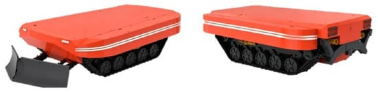
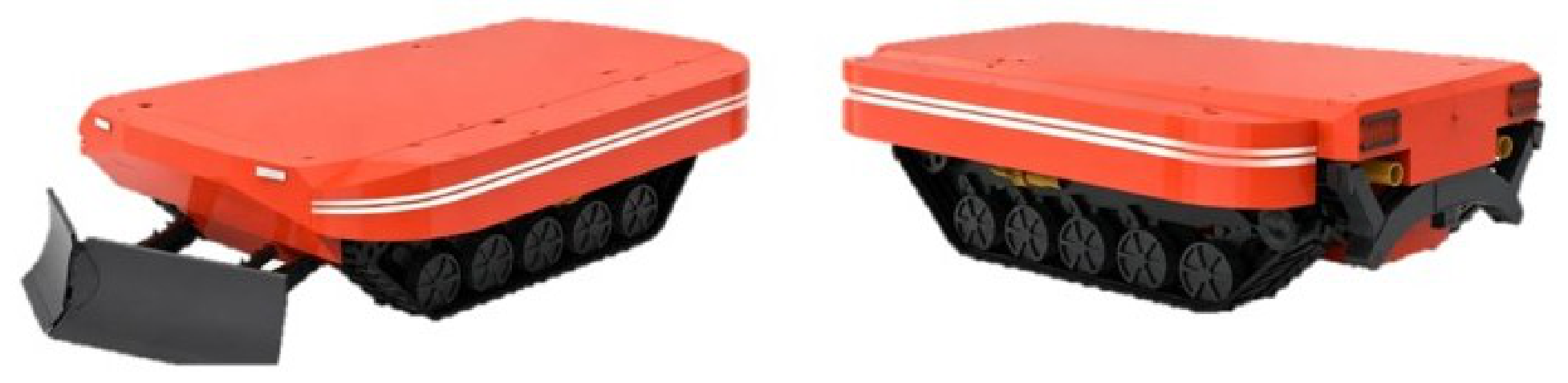
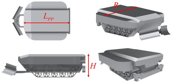
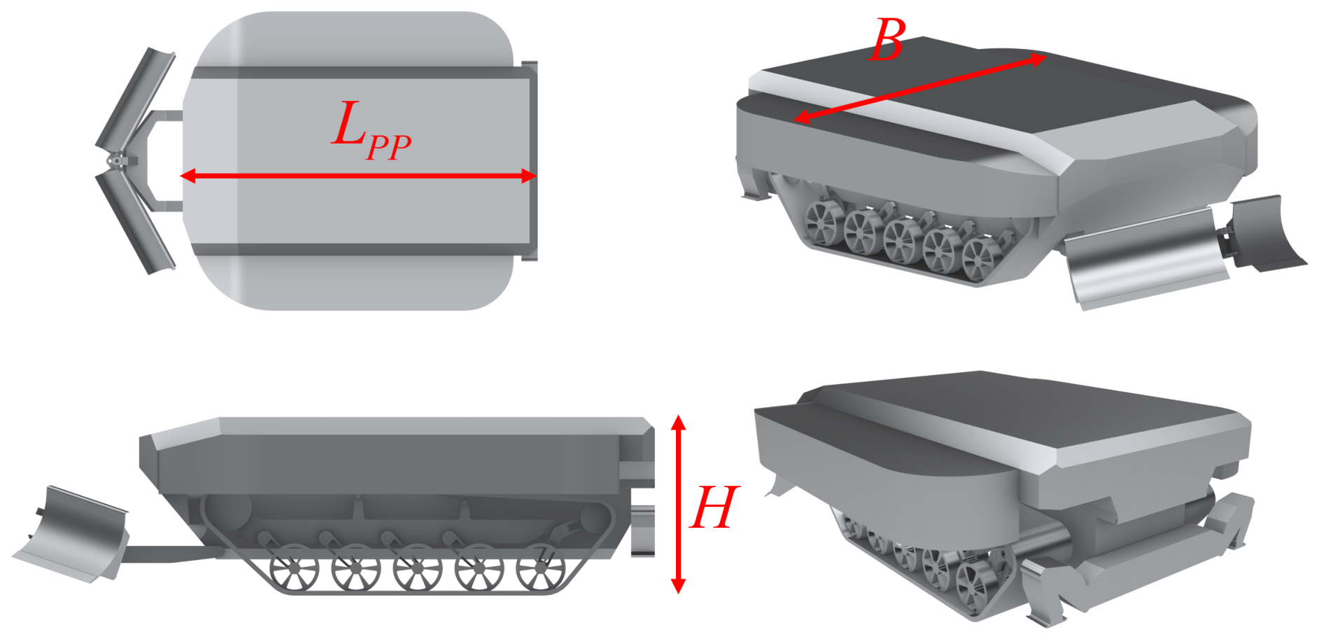
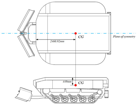
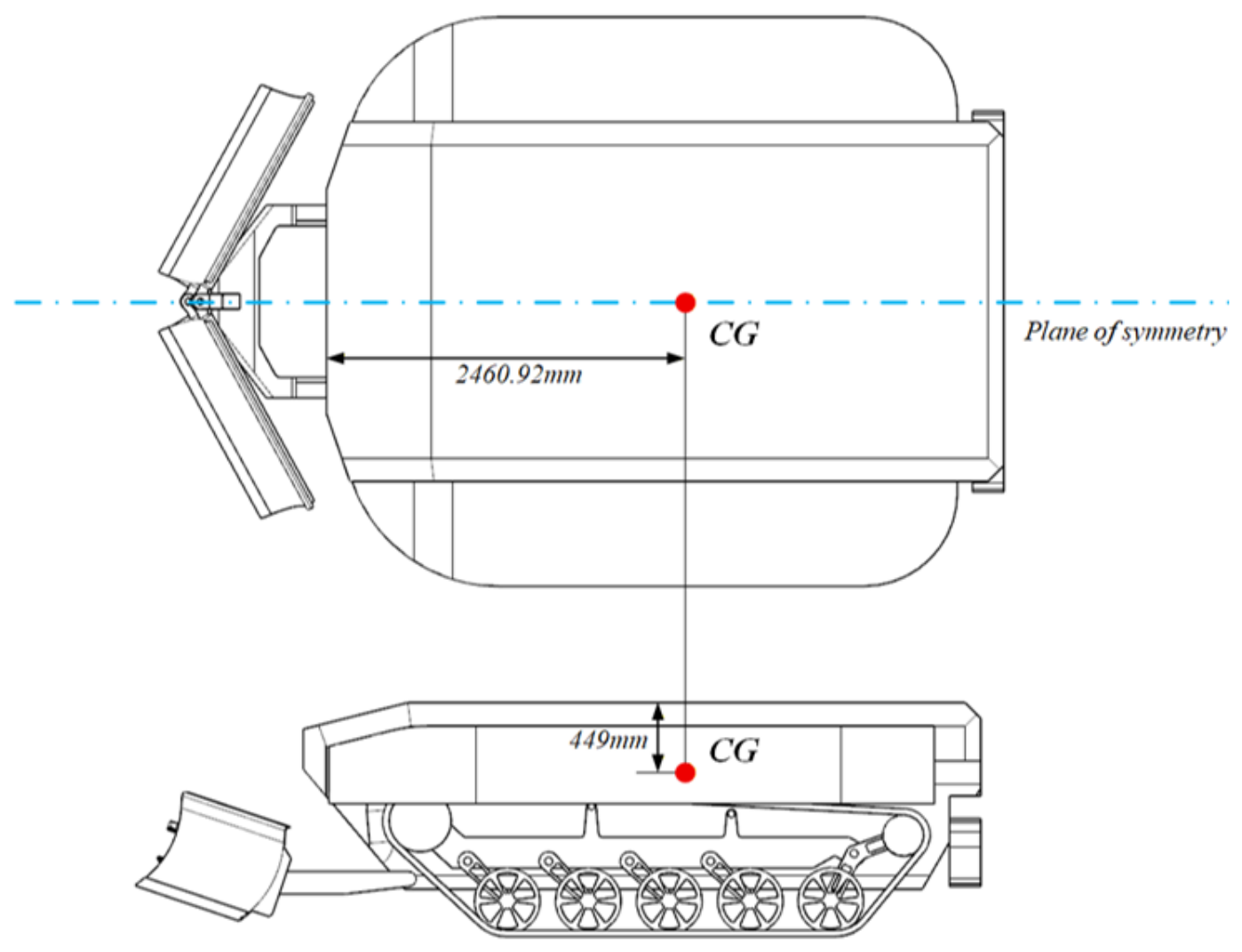
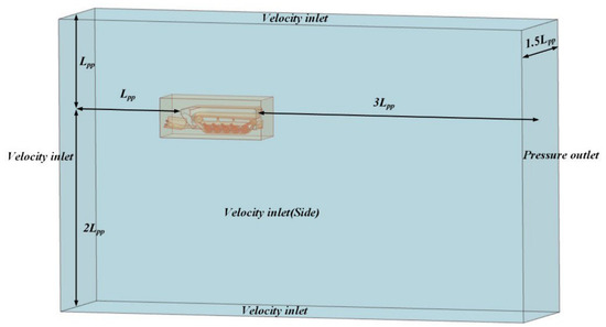
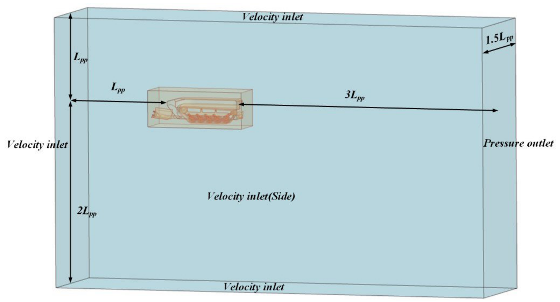
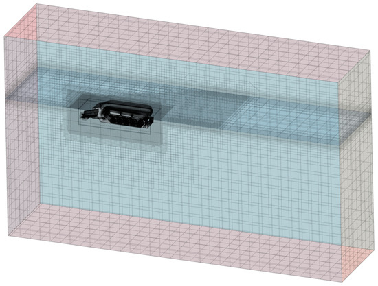
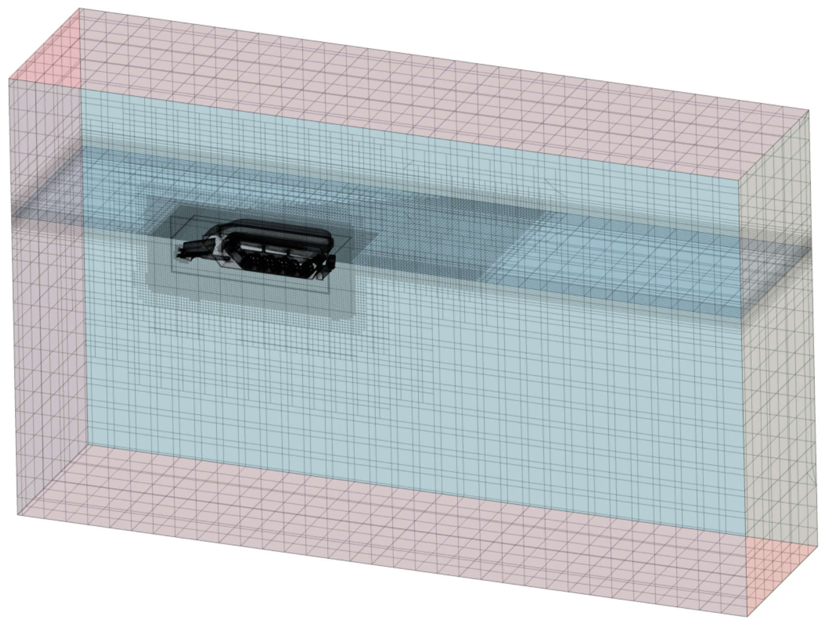
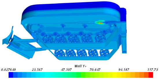
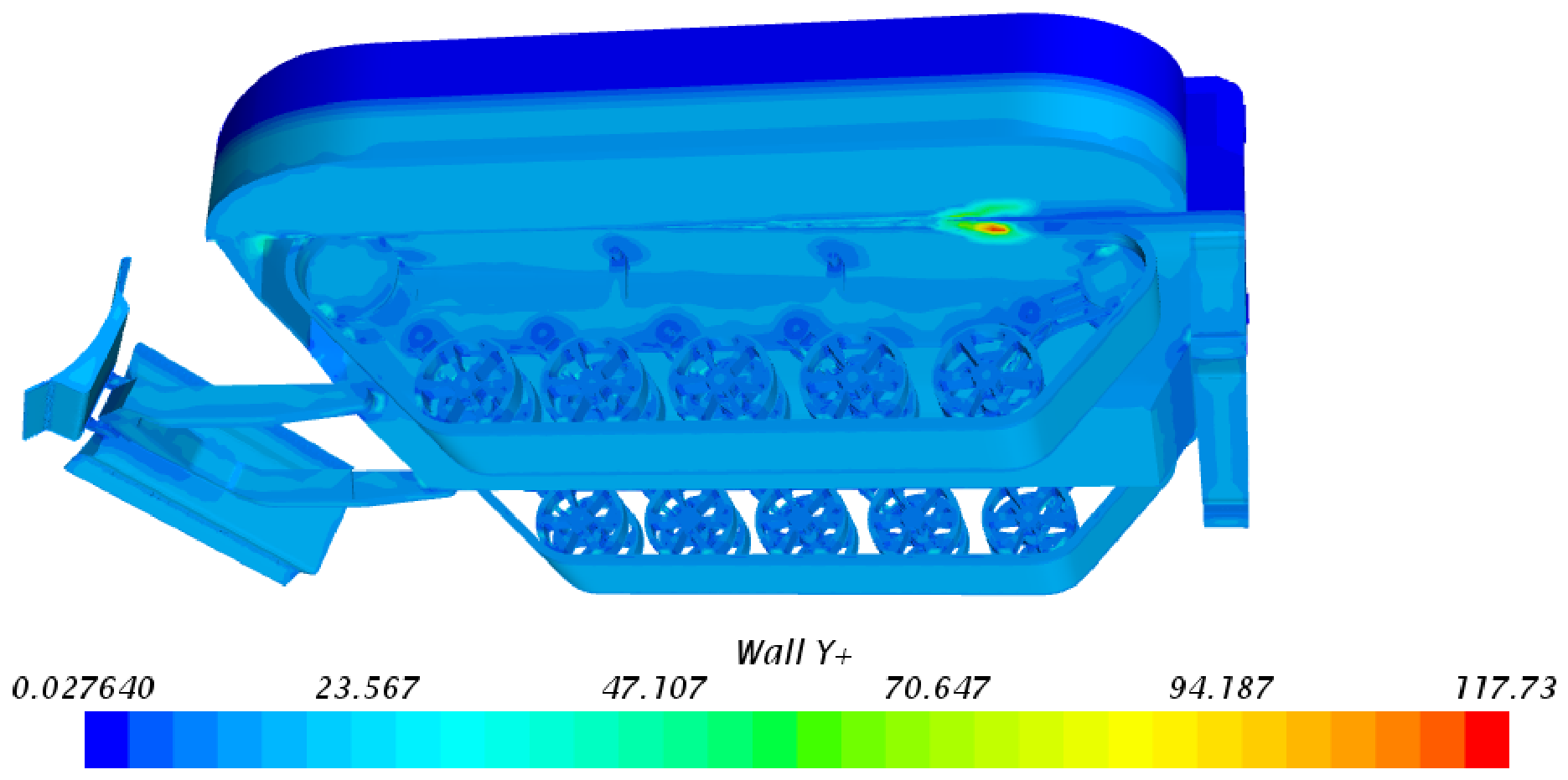
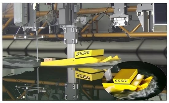
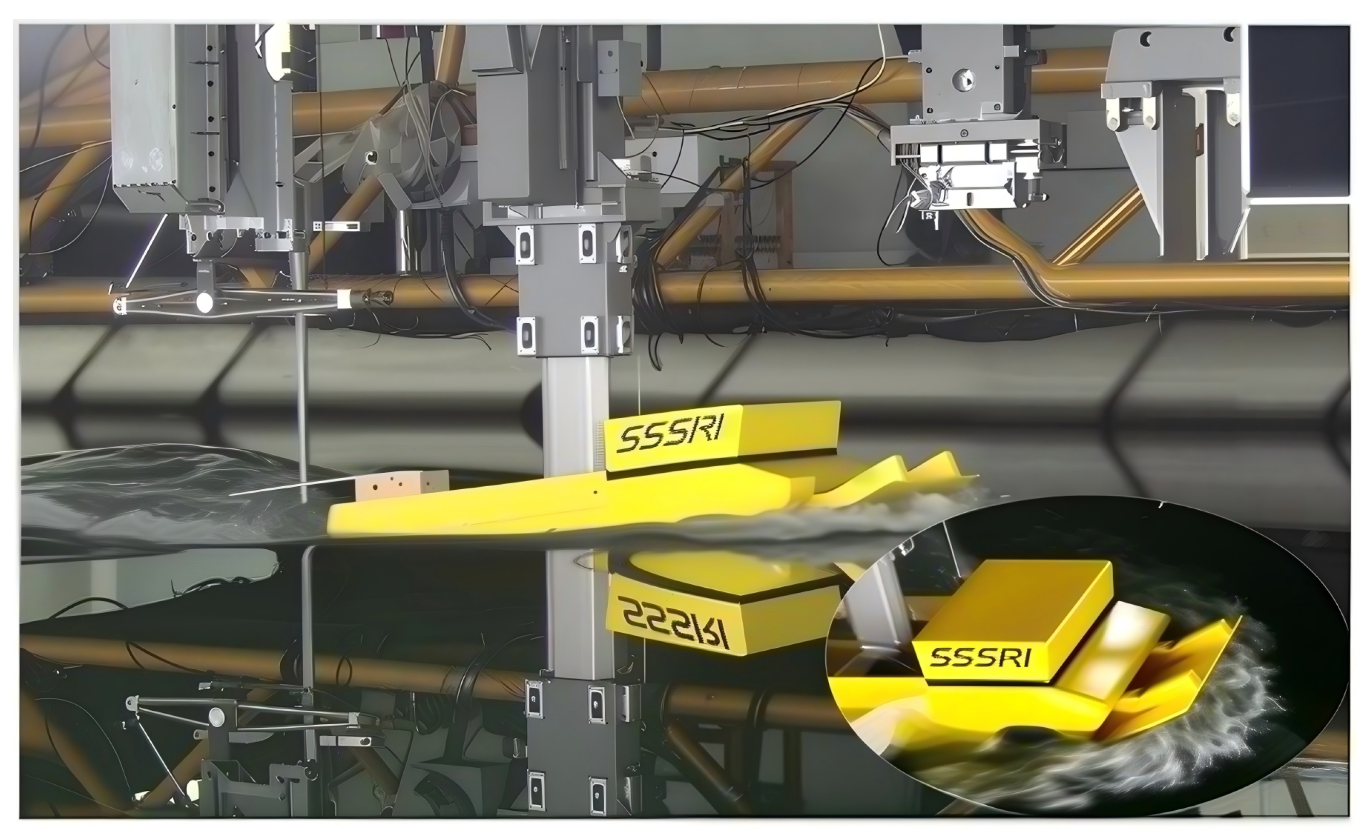
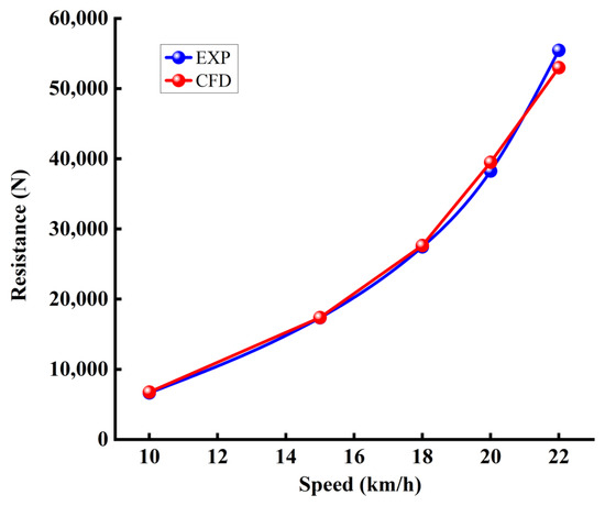
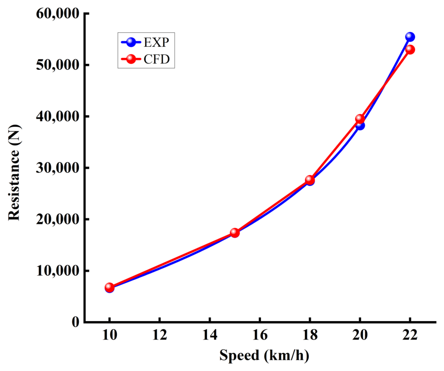
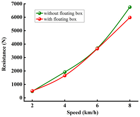
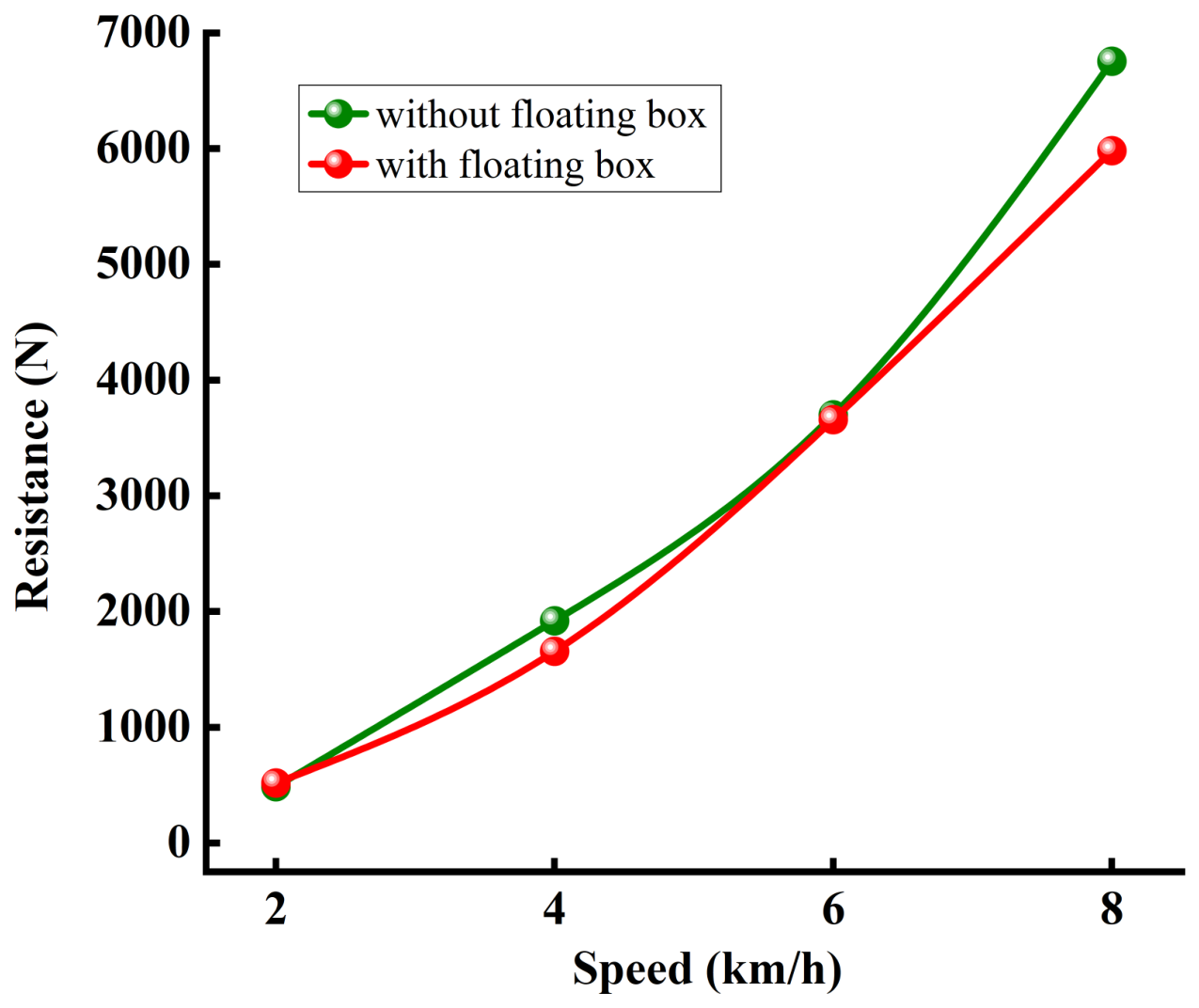
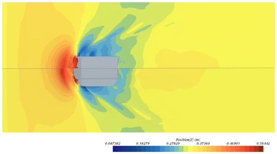
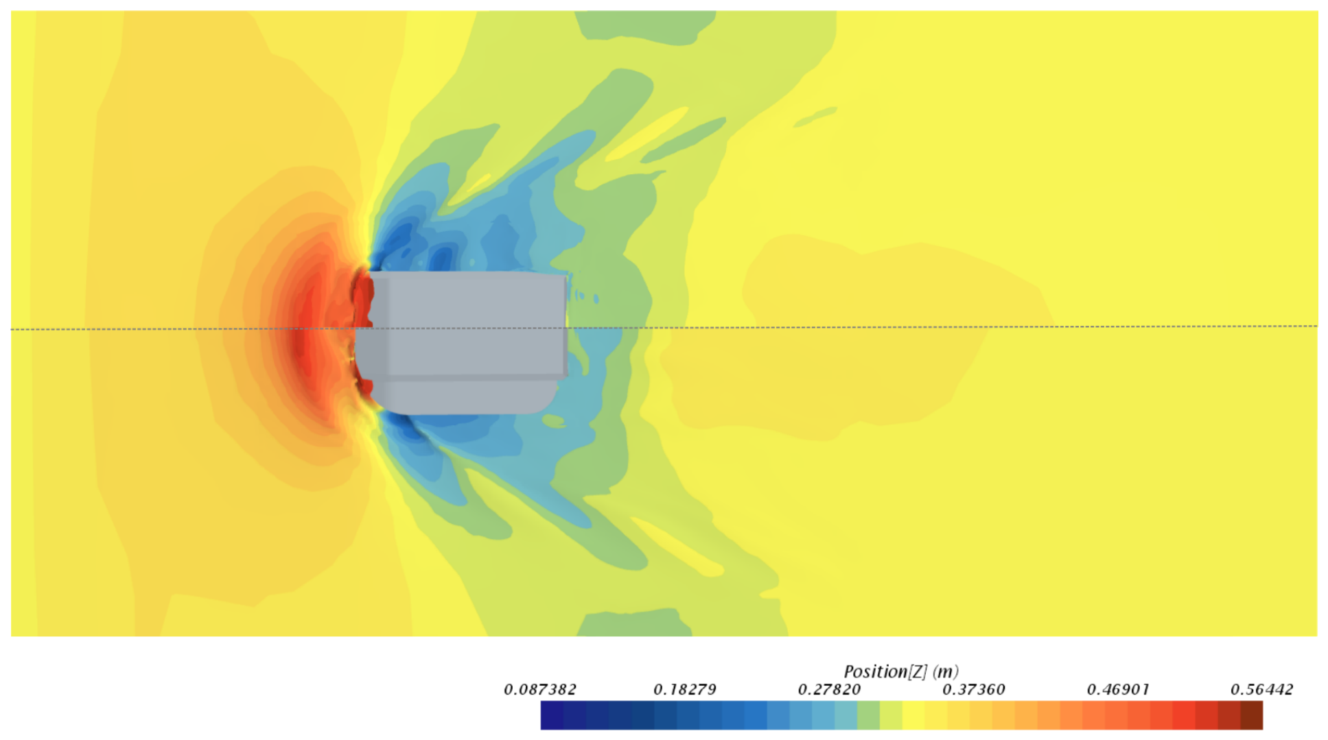
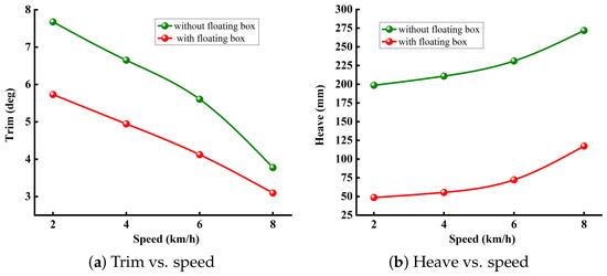
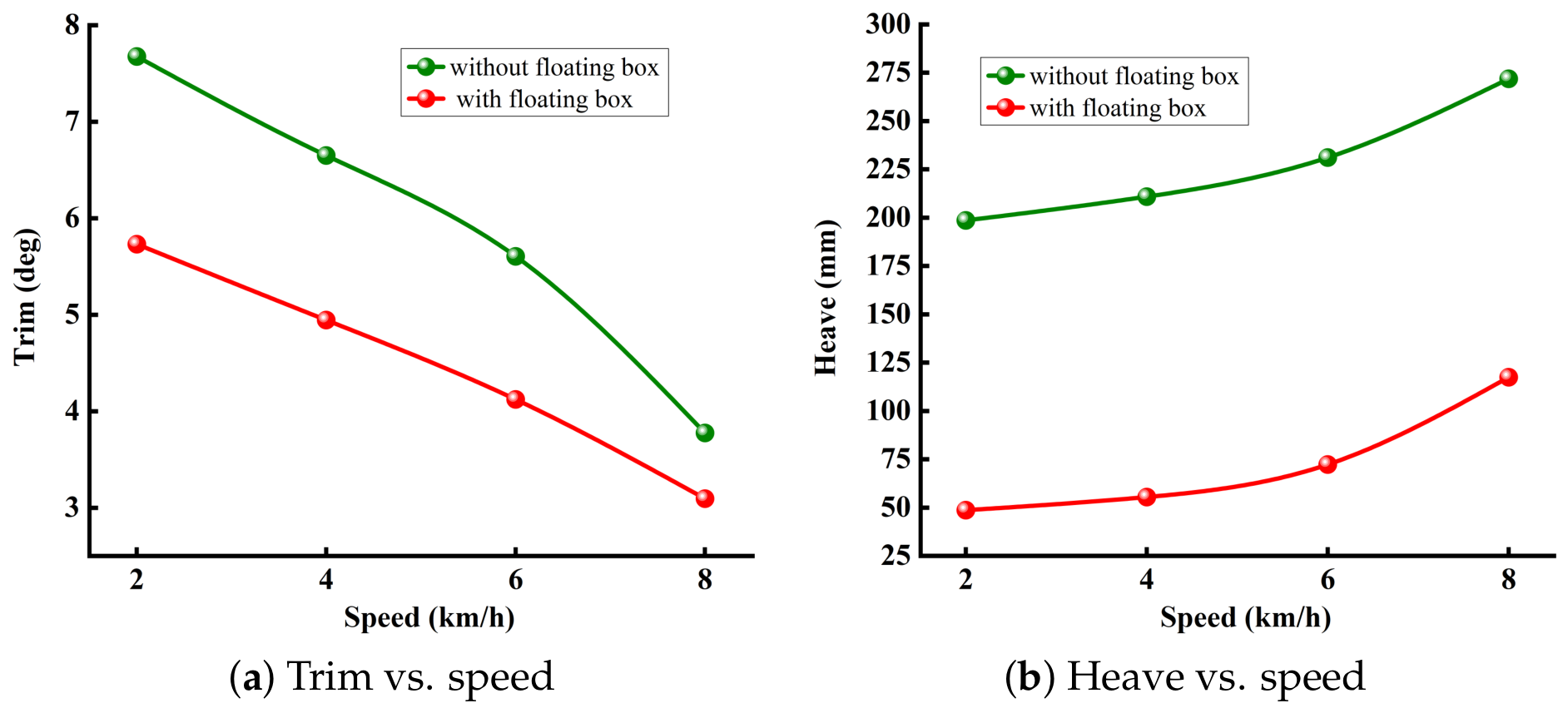
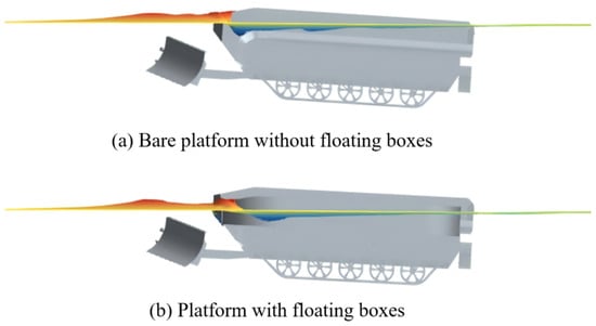
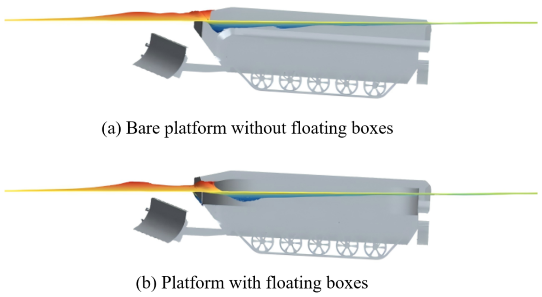
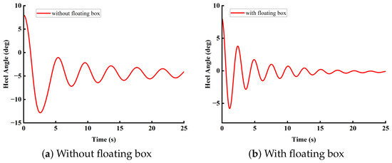
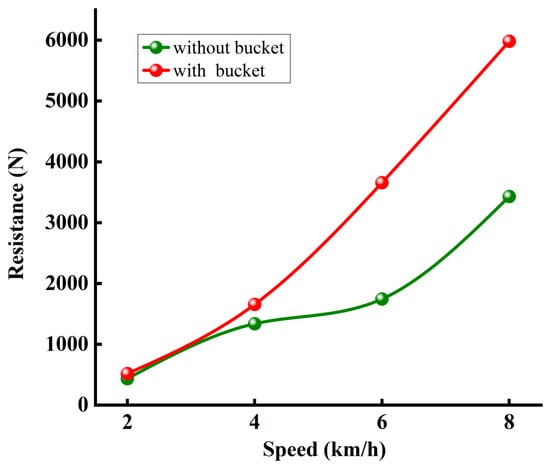
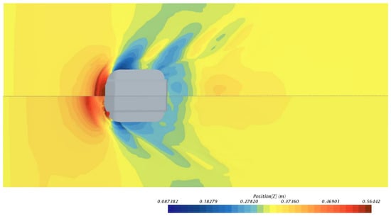
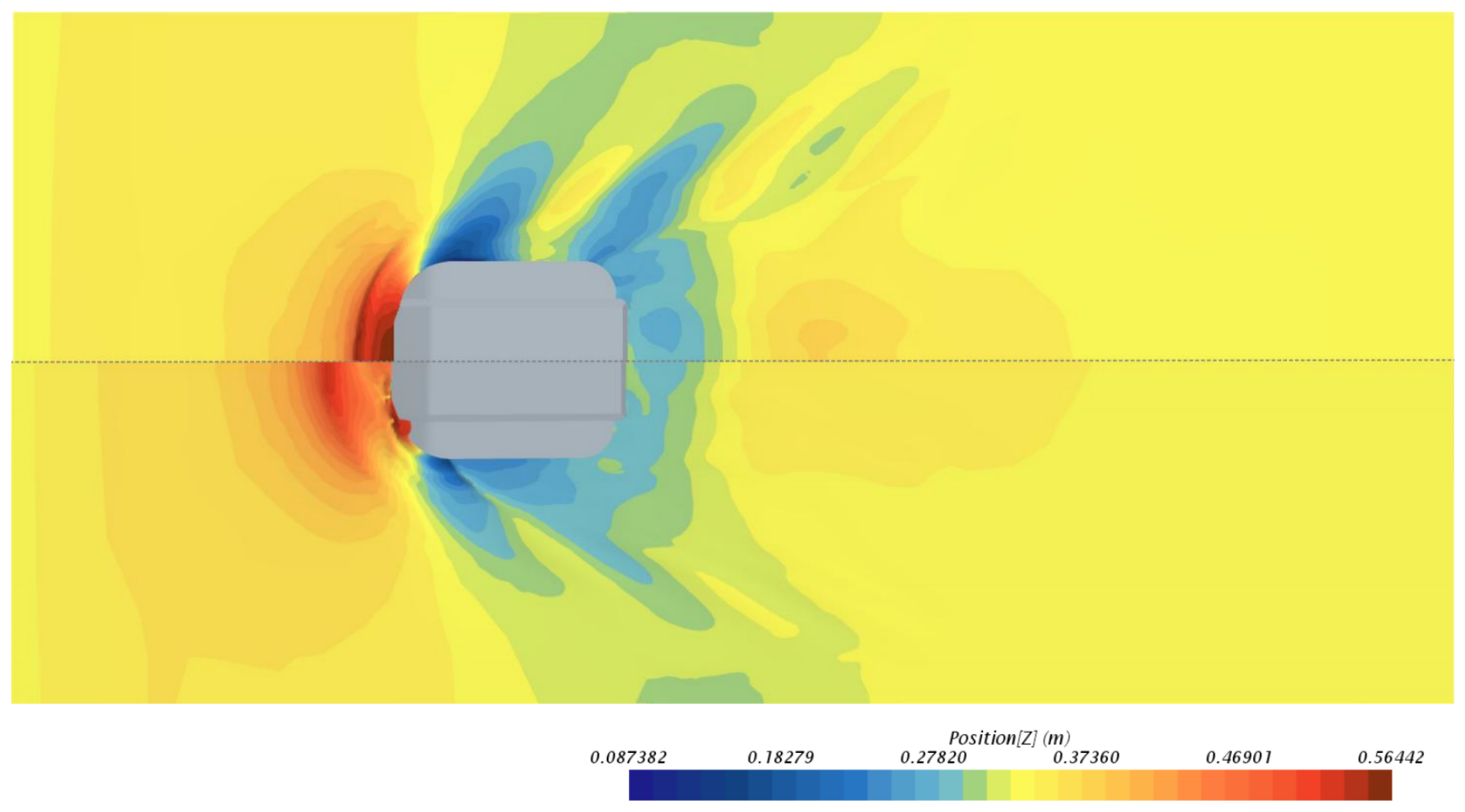
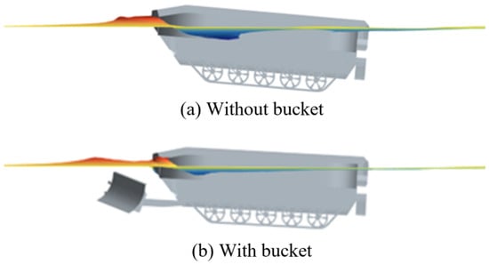
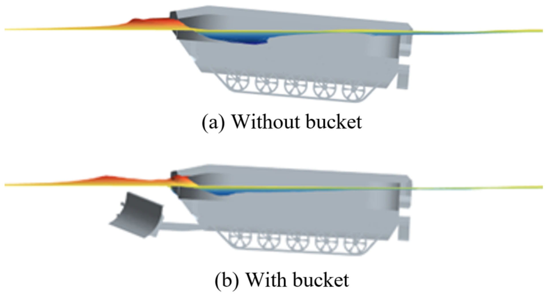
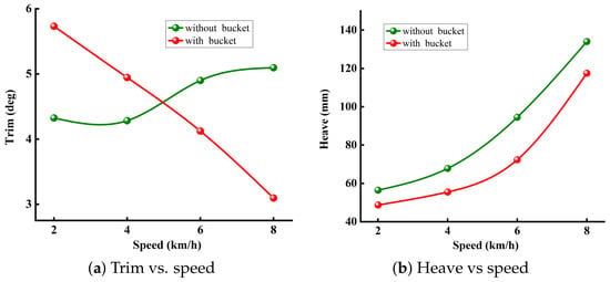
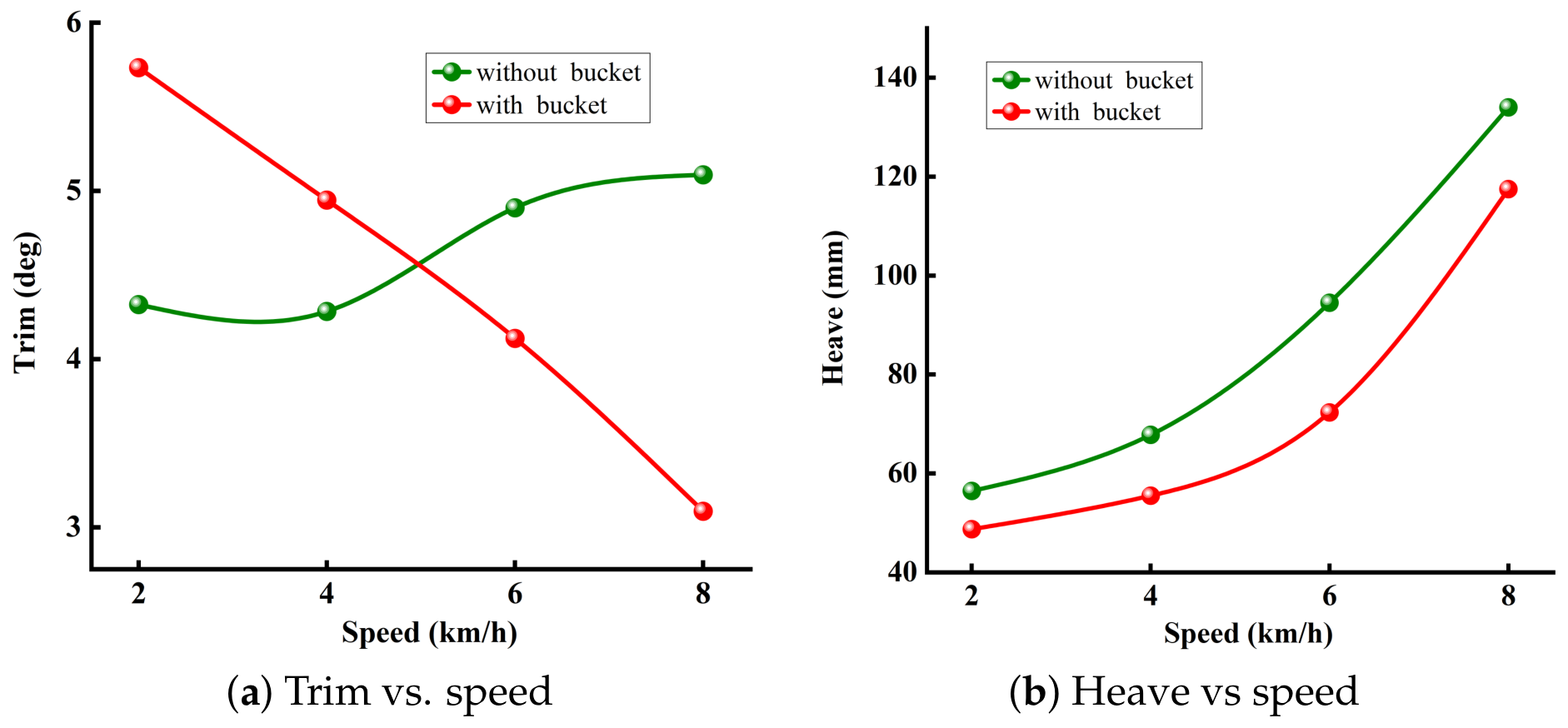
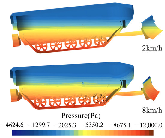
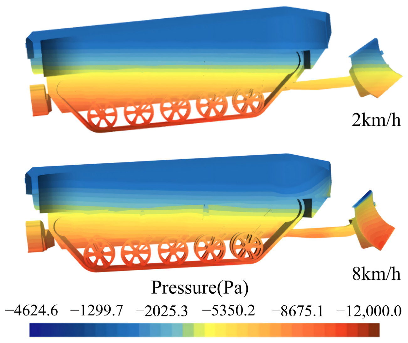
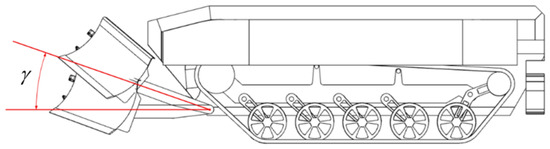
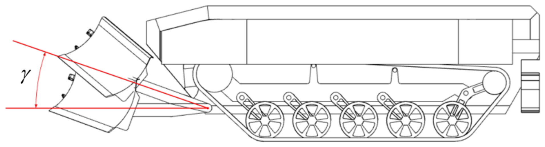
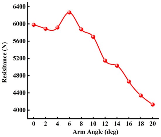
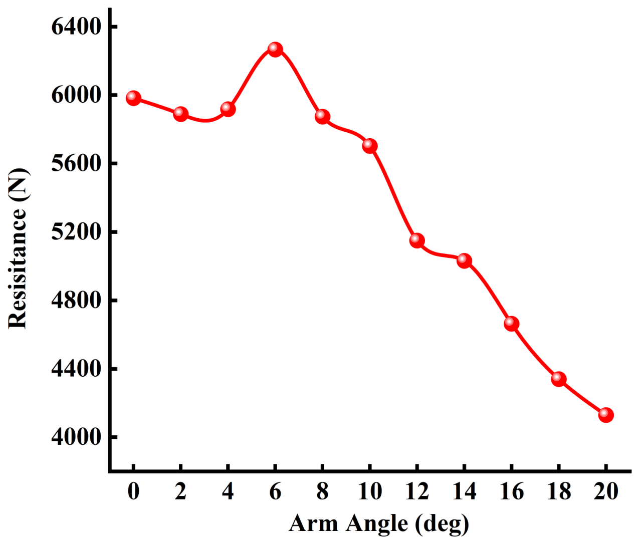
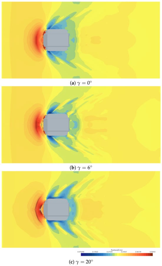
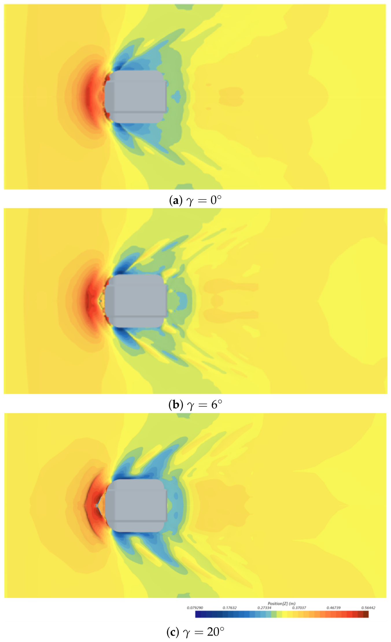
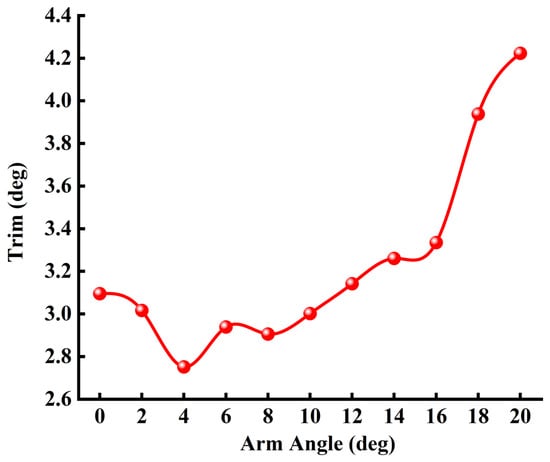
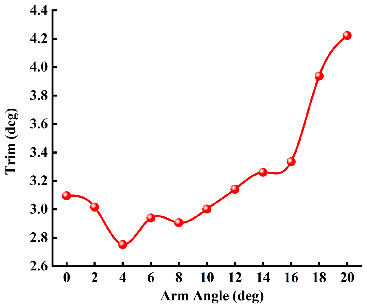
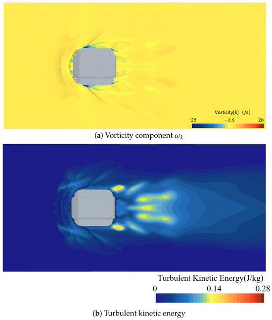
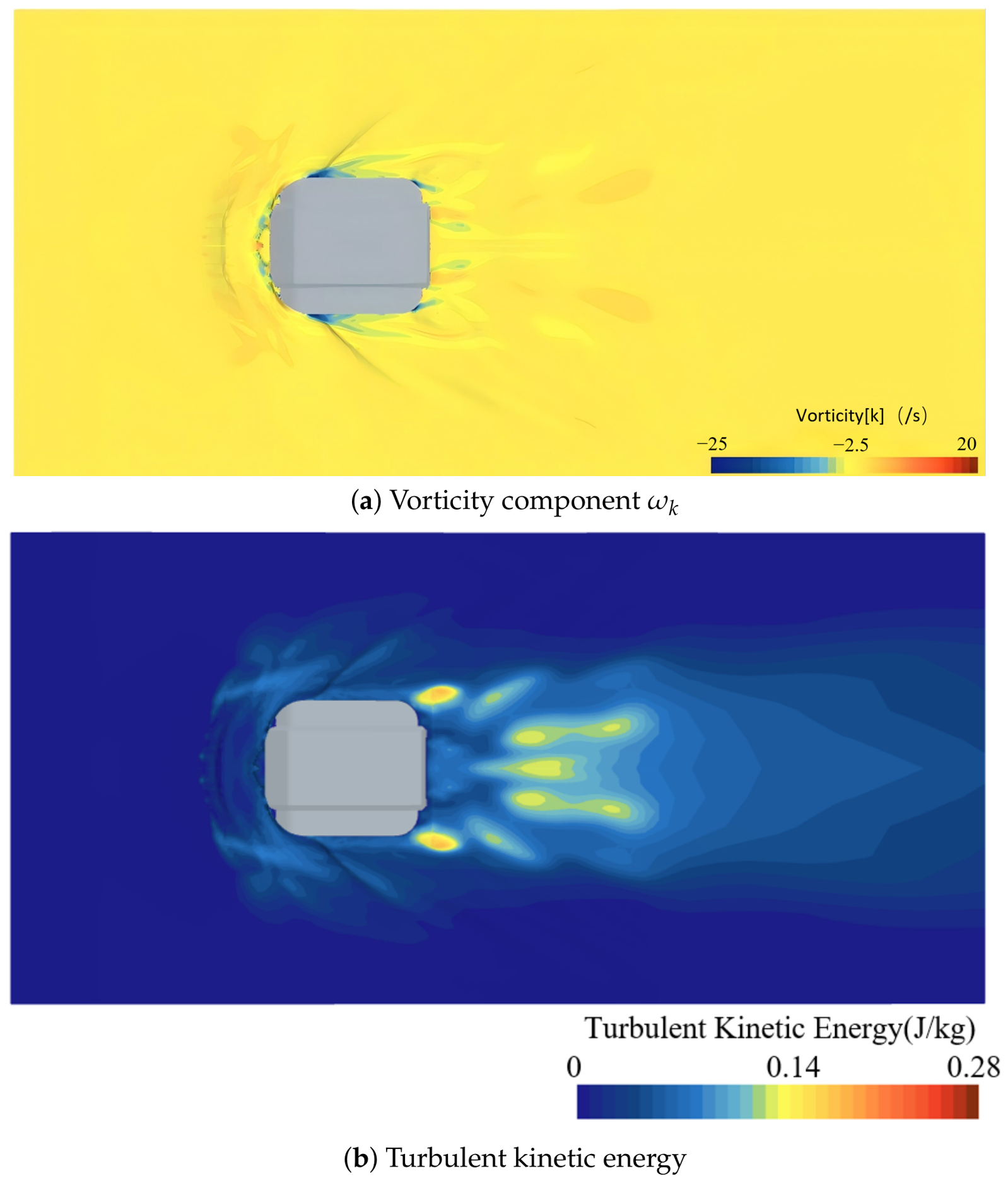
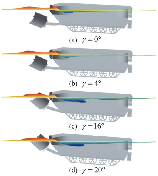
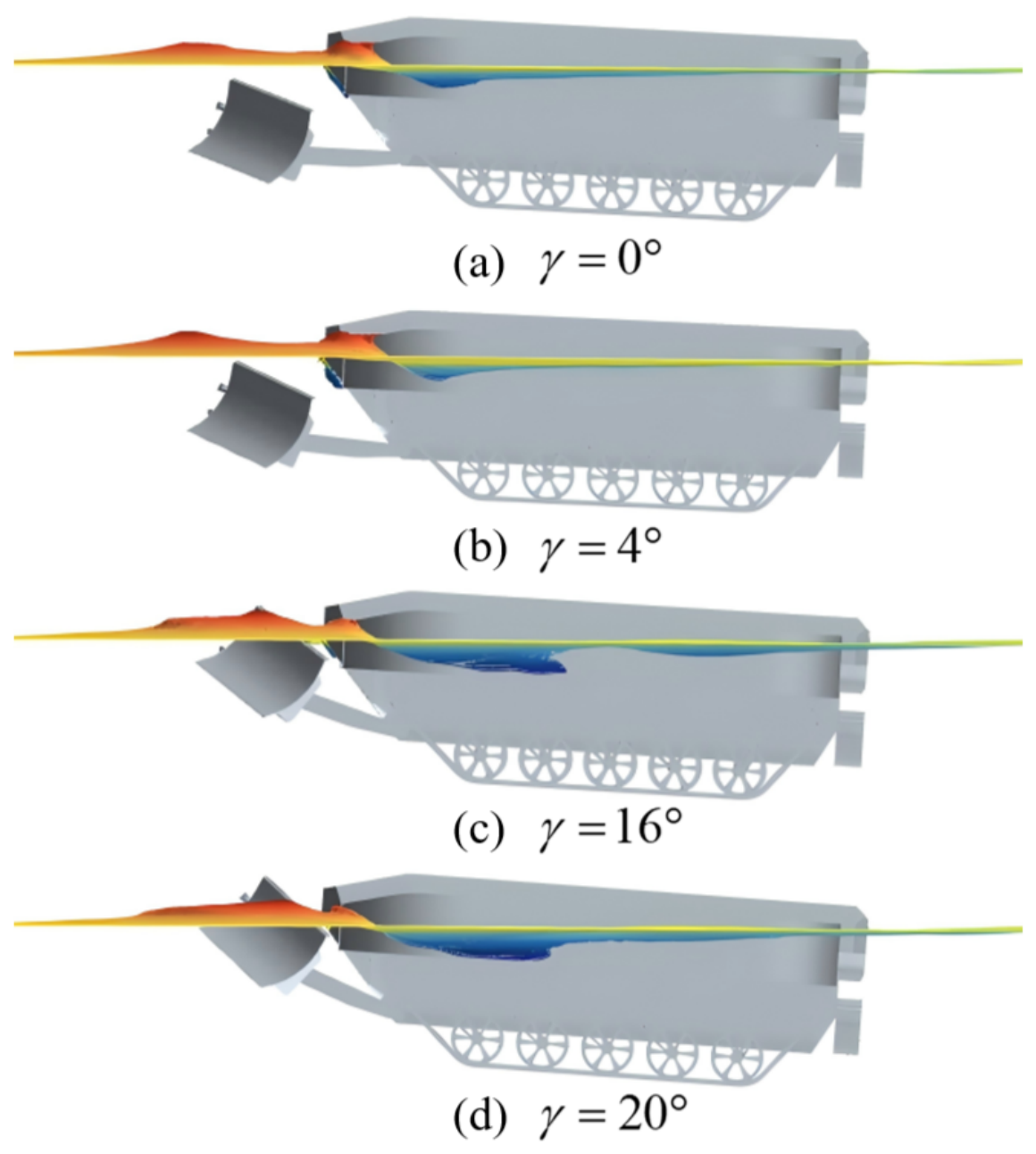
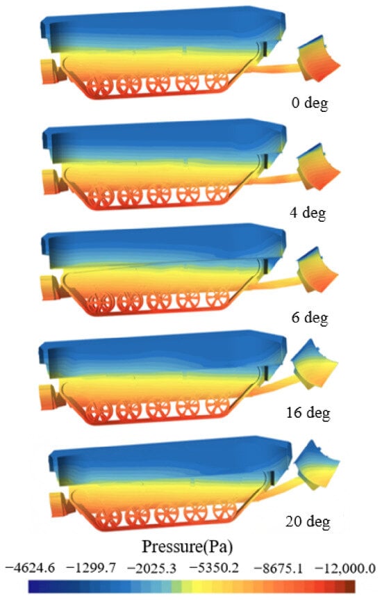
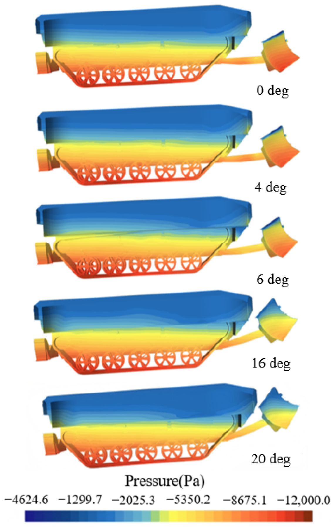
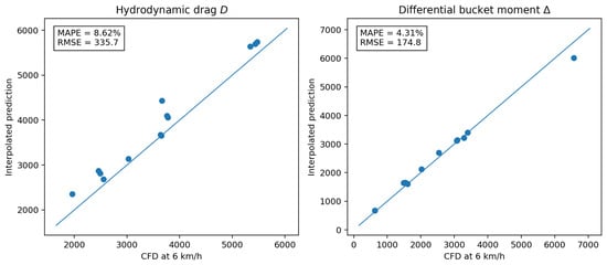
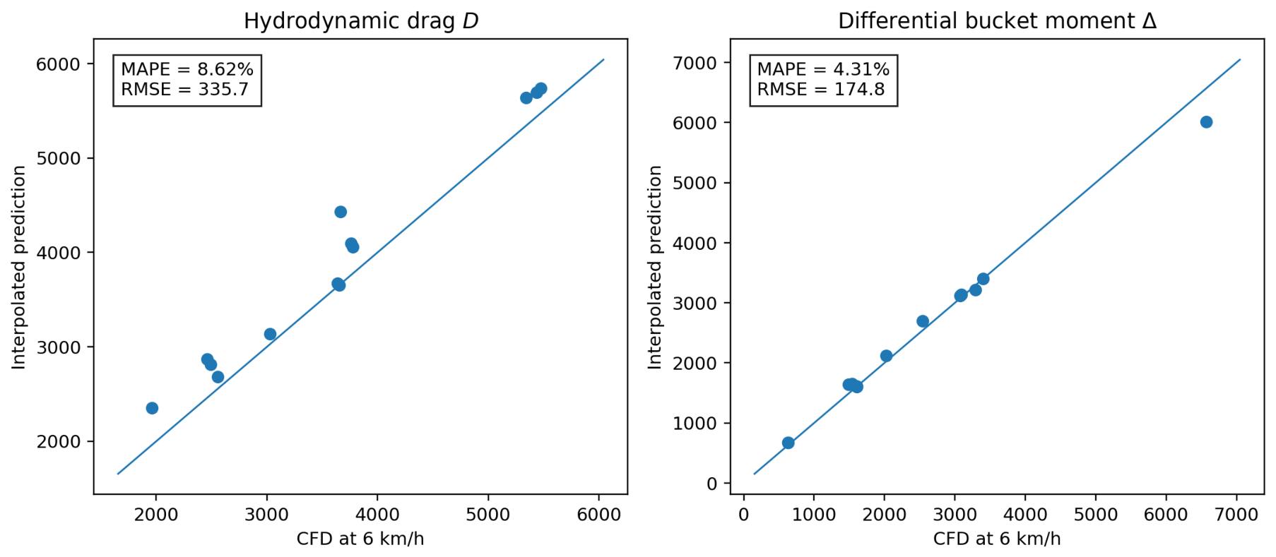
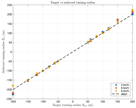
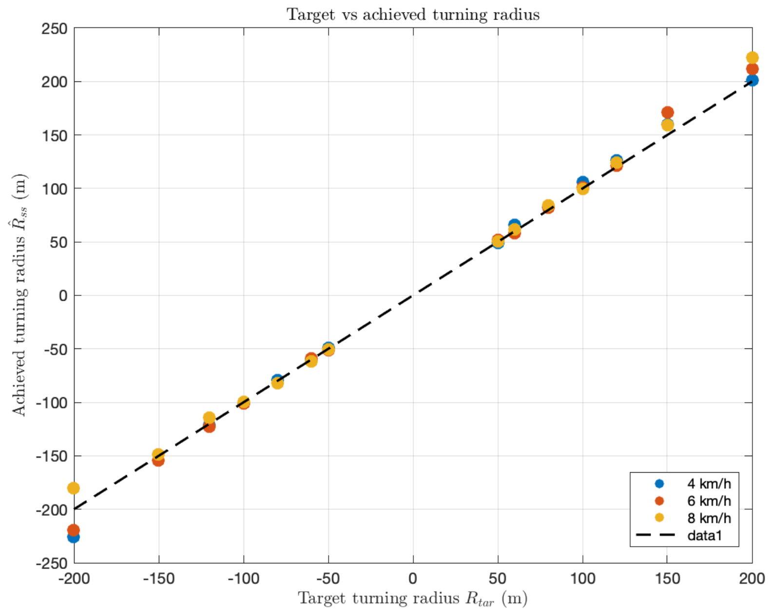
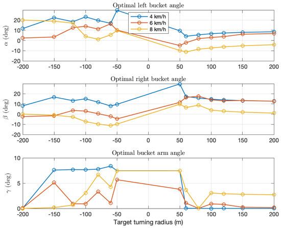
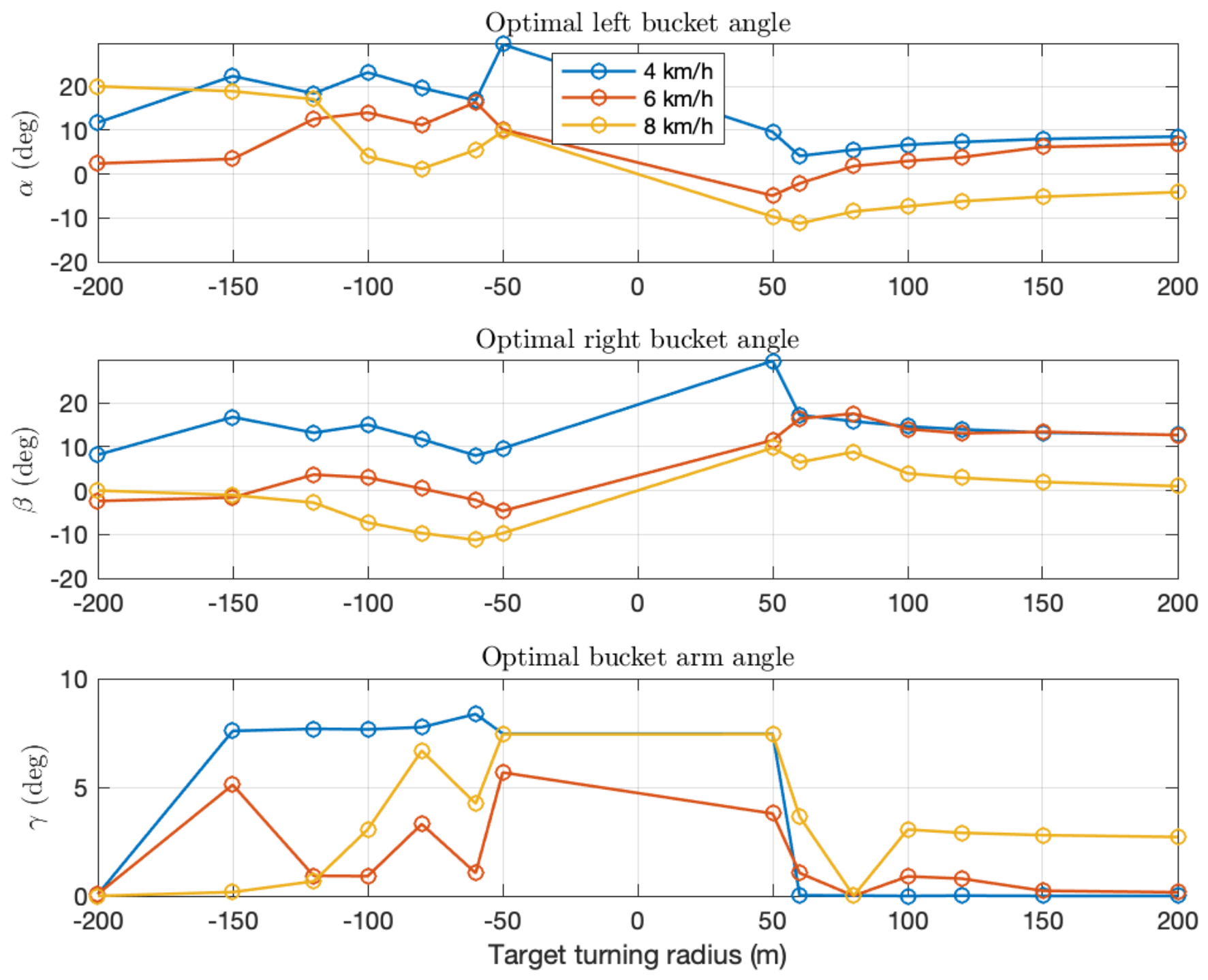
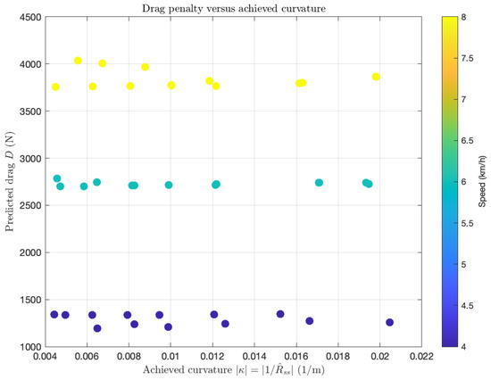
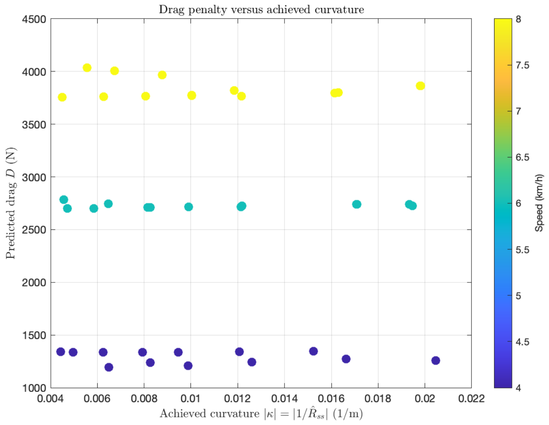
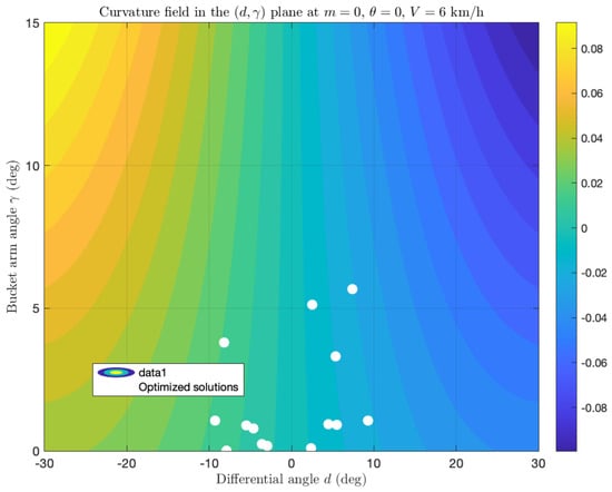
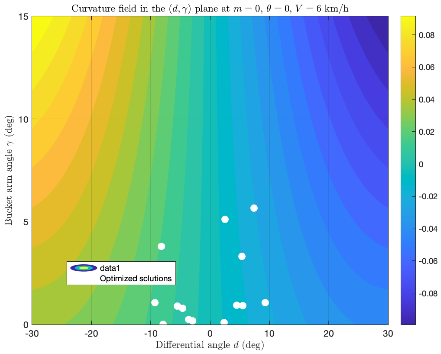
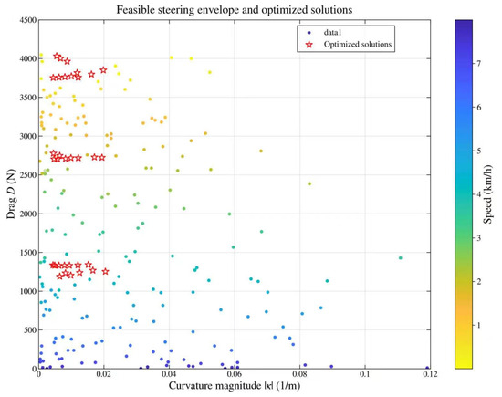
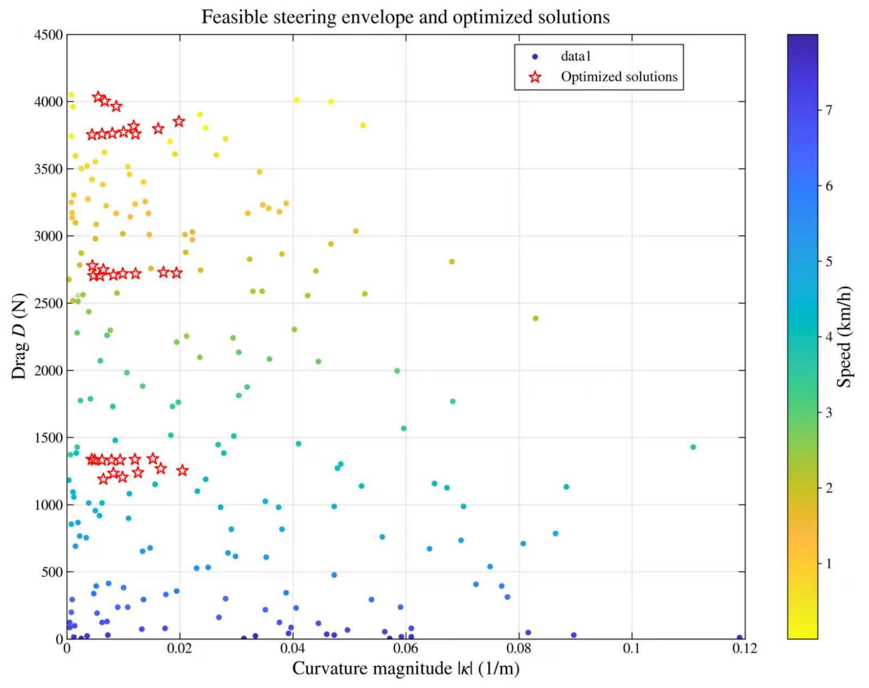
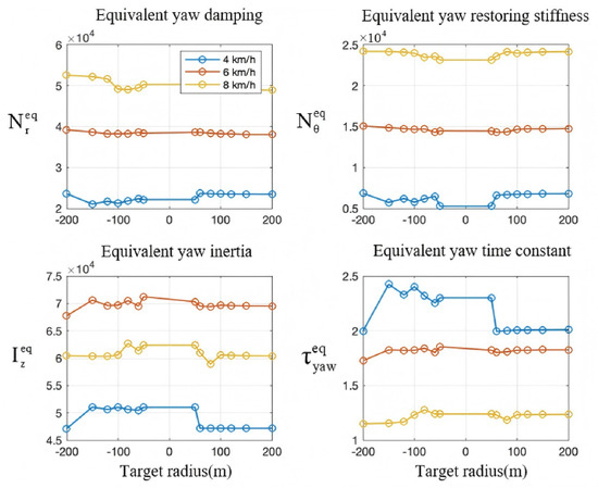
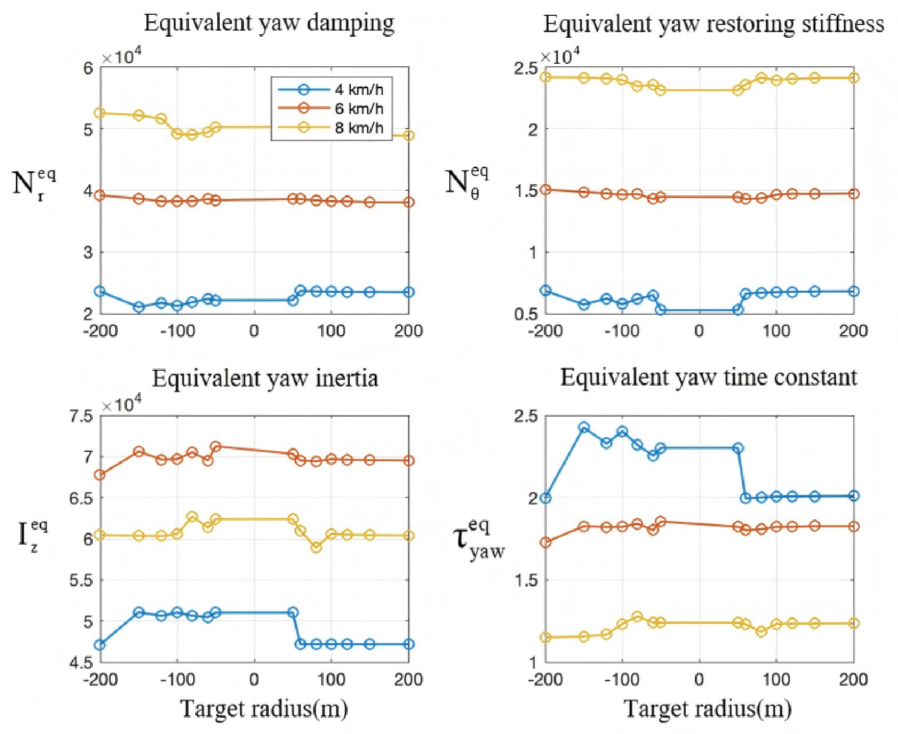

Disclaimer/Publisher’s Note: The statements, opinions and data contained in all publications are solely those of the individual author(s) and contributor(s) and not of MDPI and/or the editor(s). MDPI and/or the editor(s) disclaim responsibility for any injury to people or property resulting from any ideas, methods, instructions or products referred to in the content. |
© 2026 by the authors. Licensee MDPI, Basel, Switzerland. This article is an open access article distributed under the terms and conditions of the Creative Commons Attribution (CC BY) license.