Research on Safety Assurance Strategies for Offshore Transfer Operations Based on Floating Hose State Prediction

Abstract

With the vigorous development of offshore energy and mining, offshore fracturing and deep-sea mining necessitate the ship-to-ship and platform-to-ship transfer of solid particles via floating hoses. However, traditional floating hoses designed for oil transportation are inadequate for the long-term and stable conveyance of granular materials, as solid particles are prone to deposition and blockage under excessive bending. Additionally, in large-scale offshore fracturing operations, tension fluctuations in high-pressure hoses accelerate hose wear and compromise structural integrity. To address these challenges, this study proposes a systematic framework integrating neural network prediction with a feedforward–feedback composite control strategy. Spatial Attention–Convolutional Neural Network (SA-CNN) achieves the highest prediction accuracy and the strongest generalization capability across all operating conditions. Then, a feedforward–feedback composite control strategy is formulated, where the feedforward component is derived from SA-CNN predictions and the feedback component is provided by a PID controller, with an adaptive weighting mechanism adjusting their contributions based on prediction confidence. A curvature safety constraint is also incorporated to prevent excessive bending. The results show that the composite control strategy achieves the highest peak tension reduction, while achieving the lowest RMSE. Unlike pure PID, which introduces severe oscillations, the composite control strategy converges smoothly, confirming that feedforward prediction effectively suppresses feedback-induced oscillations. This study provides a theoretical foundation and a practical solution for the safety assurance of floating hoses in high-pressure fracturing fluid delivery applications and offshore solid particle transshipment.

1. Introduction

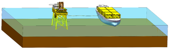
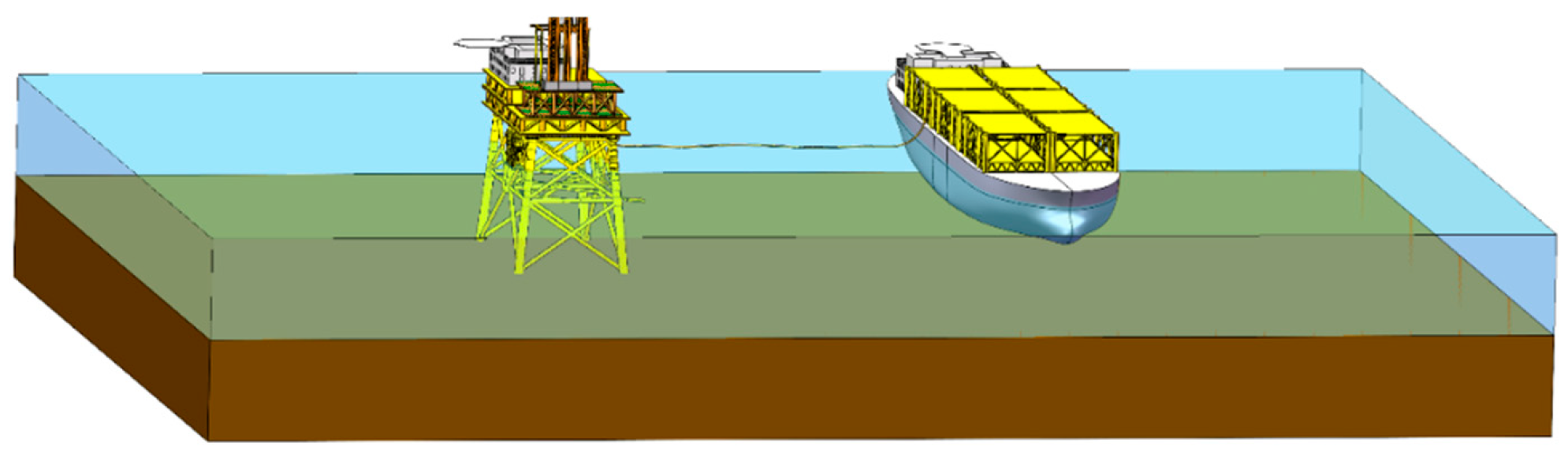
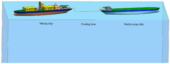
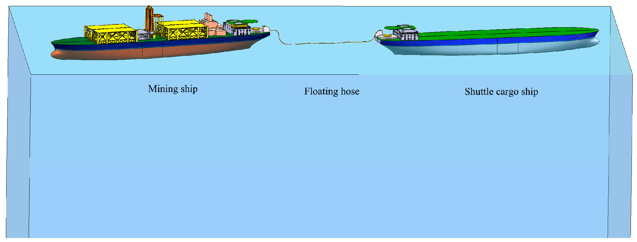
With the continuous deepening of marine resource development, the demand for solid particle transshipment between ships and platforms has become increasingly frequent and diverse, as shown in Figure 1 and Figure 2. Traditionally, floating hose transportation technology has focused mainly on liquid media such as crude oil, thus forming a relatively mature technical system [1]. However, with the advancement of strategic tasks such as offshore reservoir reform, offshore mineral production and deep-sea mining, the long-term safe transportation of solid particle materials has become a technical bottleneck to be overcome [2,3]. Furthermore, in the scenario of large-scale fracturing operations at sea, the use of a fracturing vessel to pump high-pressure fluid containing proppants (solid particles) to the platform offers significant advantages. This process requires ensuring that the floating hose has controllable tension and curvature.

Figure 1. Ship-to-platform high-pressure fracturing fluid delivery.

Figure 2. Ship-to-ship solid particle transshipment.

The typical structure of a floating hose, from the inside out, includes an anti-corrosion coating, an inner core layer, a middle rubber layer, an outer cord layer, a spiral reinforcing bar and an outer rubber layer [4]. When used for transporting solid particles—especially those with larger particle sizes or higher concentrations—the hose is prone to particle deposition, as the solids tend to settle within the pipeline [5]. When the hose undergoes excessive bending or local small-radius bends due to wave action, the particle flow velocity may be reduced, causing clogging and eventually forming blockages, which are extremely difficult to clear [6]. The design of the existing floating hose system mainly aims to withstand loads rather than actively control the shape. Its shape on the water surface is completely determined by buoyancy configuration, environmental loads and passive constraints at both ends, lacking an active mechanism to maintain a low curvature shape. Moreover, current floating hose technology lacks intelligent adjustments to adapt to changing sea conditions. The hose tension is a key factor affecting its wear life [7]. Under the action of wind, waves and currents, complex relative motions occur between the platform and the vessel, causing drastic fluctuations in the tension of the connected hose. Excessive tension accelerates the wear of the inner wall of the hose and increases the fatigue risk at the connection point; too little tension causes the hose to sag excessively, increasing the curvature and inducing blockages [8]. Most existing systems are unable to respond to such dynamic changes in real time and cannot maintain the tension within the optimal range with sufficient precision and stability [9].

However, a time-domain simulation based on the finite element method often requires a large amount of time and computational cost [10,11]. With their strong nonlinear fitting ability and fast response, artificial intelligence models have been increasingly applied in marine engineering [12]. In recent years, some researchers have begun to introduce these models into the research on the response prediction of marine flexible pipes [13,14]. Mao et al. [15] proposed a deep neural network (DNN) method to predict the dynamic tension under a mooring line failure condition and verified the feasibility and adaptability of their DNN model using actual sea state data. Yan et al. [16] developed an LSTM-based method for predicting the top tension response of umbilical cables. They compared the predictions with finite element results and verified the efficiency and accuracy of their model. Ye et al. [17] proposed an end-to-end model based on an attention-enhanced convolutional neural network (CNN) for the prediction of mooring line tension, demonstrating that the attention mechanism improves prediction performance compared to the baseline CNN.

Meanwhile, PID and its variants have been widely applied in the tensioning control of offshore hoses, risers and mooring systems. For hose tensioning, PID controllers have been adopted for the precise speed control of winch systems to maintain a constant array hose tension during deployment and recovery operations [18]. For tension control in hose manufacturing, Li et al. [19] proposed a constant tension control system based on an integral separation fuzzy PID algorithm, reducing the tension fluctuation range by nearly 40% and improving the manufacturing quality of tensile armor layers. For riser tensioner systems, Wang et al. [20] designed a PID control algorithm for anti-recoil main valve opening, successfully controlling the riser recoil speed within a reasonable range during emergency escape scenarios. For Tension Leg Platforms under mooring line failure conditions, Wang et al. [21] developed an active control scheme based on platform motion response, demonstrating that the adaptive fuzzy PID control method exhibits stronger robustness than traditional PID control.

Despite these advances, the existing research on the prediction of engineering physical quantities [15,22,23,24] focuses on the use of DNN, LSTM, Transformer and so on. The spatial attention mechanism proposed in this study explicitly weights the most informative spatial–temporal positions in the 6-DOF motion data, which enhances prediction accuracy under varying sea conditions. In addition, most existing studies concentrate on either neural network prediction or active tensioning control in isolation [9,25,26]. The integration of neural network prediction with adaptive PID control for floating hose tensioning remains underexplored. This study leverages neural network models to predict hose tension and curvature and then designs an intelligent tensioning system based on a feedforward–feedback strategy, forming an offshore hose system that can actively and intelligently control the spatial shape and tension of the hose. This represents not only an innovation in hose design but also an upgrade in system integration and control concepts. This study aims to provide a theoretical basis and practical reference for the collision avoidance and safe operation of vessels during offshore hose transfer operations.

2. Technical Solution Method

The core idea is to abandon the traditional passive suspension mode and instead sense the six-degree-of-freedom (6-DOF) ship motions, predict the future changes in hose tension and curvature, and use an intelligent tensioning system based on a feedforward–feedback strategy to regulate the hose, thereby ensuring the safety of long-term service.

2.1. Hose Physical Model

The offshore hose is modeled as a slender flexible beam–column structure [27] subjected to axial tension, bending moment and distributed loads, including self-weight, buoyancy and hydrodynamic forces. Both ends of the hose are modeled as fixed connections. The cross-sectional area of the hose is given by

$$A={\displaystyle \frac{\pi }{4}}(D_o^2-D_i^2),$$

(1)

where $A$ represents the cross-sectional area of the hose, $D_o$ represents the outer diameter, and $D_i$ represents the inner diameter. The area moment of inertia for the annular cross-section is given by

$$I={\displaystyle \frac{\pi }{64}}(D_o^4-D_i^4),$$

(2)

where $I$ represents the area moment of inertia. The bending stiffness of the hose is given by

$$EI={\displaystyle {\sum }_{j=1}^n}{E}_j{I}_j,$$

(3)

where $EI$ represents bending stiffness, $E_j$ represents Young’s modulus of the $j$ layer material, and $I_j$ represents the area moment of inertia of the $j$ layer. The axial stiffness of the hose is given by

$$EA={\displaystyle {\sum }_{j=1}^n}{E}_j{A}_j,$$

(4)

where $EA$ represents axial stiffness, and $A_j$ represents the cross-sectional area of the $j$ layer. The relationship between axial tension, $T$, and hose length, $L$, follows Hooke’s law for the composite structure

$$T=EA·\epsilon =EA·{\displaystyle \frac{\Delta L}{L_0}},$$

(5)

where $T$ represents axial tension, $\epsilon$ represents axial strain, $\Delta L$ represents the change in hose length, and $L_0$ represents the original length of the hose. Thus, for small-length adjustments, $\Delta L$, the resulting tension change, $\Delta T$, can be expressed linearly as [28]

$$\Delta T={\displaystyle \frac{EA}{L_0}}·\Delta L=K_T·\Delta L,$$

(6)

where $\Delta T$ represents the change in hose tension, and $K_T$ represents the tension sensitivity coefficient. For a slender beam, the relationship between bending moment, $M$, and curvature, $\kappa$, is governed by the Euler–Bernoulli beam theory [29]

$$M=EI·\kappa ,$$

(7)

where $M$ represents the bending moment, and $\kappa$ represents the curvature of the hose. For small deflections, the curvature, $\kappa$, can be approximated as

$$\kappa ={\displaystyle \frac{d\theta }{ds}}\approx {\displaystyle \frac{d^{2}y}{d{x}^2}},$$

(8)

where $\theta$ represents the tangent angle of the hose centerline relative to the horizontal plane, $s$ represents the arc length along the hose centerline, $y$ represents the lateral deflection of the hose, and $x$ represents the axial coordinate along the hose. The equilibrium of a differential hose element is given by

$${\displaystyle \frac{d^{2}M}{d{x}^2}}=-q\left(x\right)+T·{\displaystyle \frac{d^{2}y}{d{x}^2}},$$

(9)

where $q\left(x\right)$ represents the distributed load. Substituting Equation (8) into the equilibrium equation, the governing differential equation for the hose deflection is obtained

$$EI{\displaystyle \frac{d^{4}y}{d{x}^4}}=-q\left(x\right)+T·{\displaystyle \frac{d^{2}y}{d{x}^2}},$$

(10)

From Equation (9), the relationship between tension, $T$, and curvature, $\kappa$, is derived as

$$T\approx EI·\kappa +C,$$

(11)

where $C$ represents an integration constant. This coupling implies that changes in length adjustments affect both tension and curvature simultaneously. For a length adjustment, $\Delta L$, the resulting curvature change, $\Delta \kappa$, is calculated as [30]

$$\Delta \kappa =K_{\kappa }·\Delta L,$$

(12)

where $\Delta \kappa$ represents the change in curvature, and $K_{\kappa }$ represents the curvature sensitivity coefficient. A positive $\Delta L$ (lengthening the hose) decreases tension ($K_T<0$) but increases curvature ($K_{\kappa }>0$). This inherent physical conflict forms the basis for choosing tension as the primary control target while treating curvature as a safety constraint.

Under the combined action of tension, buoyancy and self-weight, the offshore hose assumes a catenary configuration [31]. The parameter relationship is described by the catenary equation

$${\displaystyle \frac{dT}{ds}}=wcos\theta ,$$

(13)

where $w$ represents the distributed weight per unit length. The curvature, $\kappa$, is given by

$$\kappa ={\displaystyle \frac{d\theta }{ds}}={\displaystyle \frac{wsin\theta }{T}},$$

(14)

2.2. Spatial Attention–Convolutional Neural Network

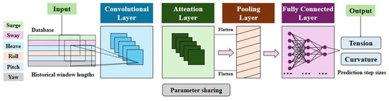
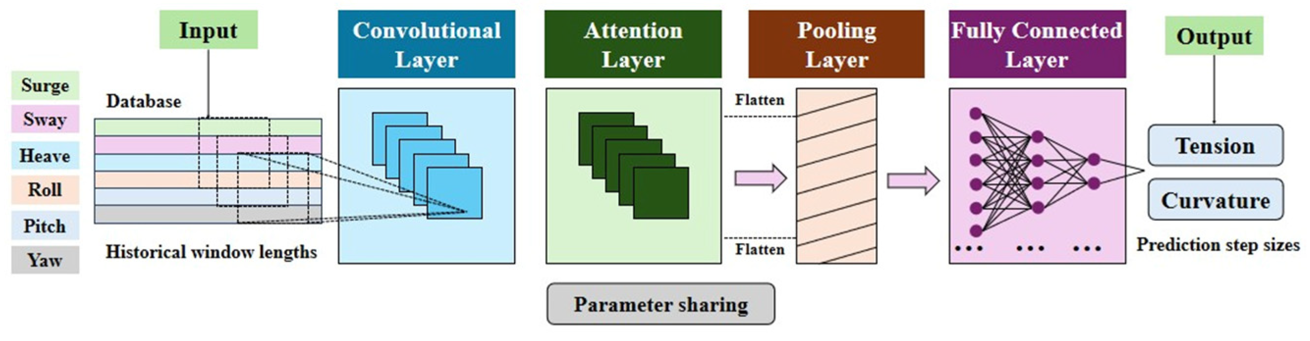
The use of attention mechanisms combined with CNN has proven effective in other safety-critical prediction tasks. For instance, a multi-head attention-enhanced CNN combined with reinforcement learning has been successfully applied to autonomous circuit synthesis and performance prediction in complex design spaces [32]. Inspired by this, the present study introduces a spatial attention mechanism into a pure CNN to construct a spatial attention–convolutional neural network (SA-CNN) architecture. As shown in Figure 3, SA-CNN introduces an additional attention layer compared to the standard CNN, guiding the network to allocate its limited computing resources to the local areas that are more discriminative for the prediction task, thereby suppressing the interference from background noise or non-key features [33].

Figure 3. Illustration of SA-CNN.

The forward computation process of SA-CNN can be summarized as follows: Firstly, the input multivariate time series is stacked to form a two-dimensional feature map, $F\in {\mathbb{R}}^{C\times H\times W}$, where $C,H,W$ represent the number of channels, time steps and variables respectively. Then, this feature map is sent to the spatial attention module to generate a spatial weight map. The calculation process of the spatial attention weights is given by [17]

$$SA=\sigma \left({conv}^{3\times 3}\right(concat\left[Avg\text{\_}CP\right(F);\mathit{M}\mathit{a}\mathit{x}\mathit{\text{\_}}\mathit{C}\mathit{P}(\mathit{F}\left)\right]\left)\right),$$

(15)

where $Avg\text{\_}CP\left(F\right)$ and $Max\text{\_}CP\left(F\right)$ respectively represent the average pooling and maximum pooling operations performed along the channel dimension, and their definitions are given by

$$Avg\text{\_}CP(F)={\displaystyle \frac{1}{C}}{\displaystyle {\sum }_{c=1}^C}F(c;·),$$

(16)

$$Max\text{\_}CP(F)=\underset{c}{\mathit{max}}F(c;·),$$

(17)

where $F(c;·)$ indicates that operations are performed on all spatial positions of a channel, $c$. After pooling and concatenation, a two-channel spatial descriptor is obtained. Then, through a $3\times 3$ convolution layer and the Sigmoid activation function, a spatial attention map, $SA\in {\mathbb{R}}^{1\times H\times W}$, with the same spatial size as the original feature map is generated. Each element of this attention map takes values in the range of $(0, 1)$, representing the importance of the corresponding spatial position.

Ultimately, the spatial attention map re-calibrates the original feature map through element-wise multiplication

$$F^{\prime }=SA⨀F,$$

(18)

where $⨀$ represents the Hadamard product. The spatial attention weights are broadcasted across all channels in the channel dimension, thereby achieving differentiated enhancement or suppression for different spatial positions.

2.3. Feedforward–Feedback Control Strategy

With the aforementioned predicted data, this study proposes a composite control strategy combining feedforward and feedback actions. The initial length adjustment command is given by

$$\Delta L\left(t\right)=u\left(t\right)=u_{FF}\left(t\right)+u_{FB}\left(t\right),$$

(19)

where $\Delta L\left(t\right)$ represents the length adjustment command, $u\left(t\right)$ represents the total control signal, $u_{FF}\left(t\right)$ represents the feedforward component, and $u_{FB}$ represents the feedback component. The feedforward action [34] is computed from the neural network predictions

$$u_{FF}\left(t\right)=K_{FF}\left(\widehat{T}\left(t+p\right)-T_{target}\right),$$

(20)

where $K_{FF}$ represents the feedforward gain, $\widehat{T}$ represents neural network predictions, and $T_{target}$ represents the target tension. The feedback action is computed using a standard PID controller [35]

$$u_{FB}\left(t\right)=K_p{e}_T\left(t\right)+K_i{\int }_0^t{e}_T\left(\tau \right)d\tau +K_d{\dot{e}}_T\left(t\right),$$

(21)

where $K_p$ represents the proportional gain, $K_i$ represents the integral gain, $K_d$ represents the derivative gain, $e_T$ represents the tension error, ${\dot{e}}_T\left(t\right)$ represents the rate of change of the tension error. To account for the varying prediction accuracy of the neural network under different sea conditions, an adaptive weighting factor, $\lambda \left(t\right)$, ref. [36] is introduced. The feedforward contribution is automatically adjusted based on the prediction accuracy, quantified by the coefficient of determination, $R^2$

$$\lambda (t)={\displaystyle \frac{R^2\left(t\right)}{R^2\left(t\right)+\alpha }},$$

(22)

where $\lambda$ represents the adaptive weighting factor, $R^2$ represents the coefficient of determination, and $\alpha$ represents a smoothing parameter to prevent $\lambda$ from reaching 1. The final control signal, $u\left(t\right)$, is calculated as a weighted combination of the feedforward and feedback components

$$u\left(t\right)=\lambda \left(t\right)·u_{FF}\left(t\right)+(1-\lambda \left(t\right))·u_{FB}\left(t\right),$$

(23)

Tension is the primary control target, and curvature is monitored as a safety constraint. When the curvature exceeds the safety threshold, ${\kappa }_{safe}$, the control action is automatically attenuated. The decay factor, $d\left(t\right)$, ref. [37] is defined as follows:

$$d(t)=\max \left(d_{min},1-{\displaystyle \frac{\kappa (t)-{\kappa }_{safe}}{{\kappa }_{max}-{\kappa }_{safe}}}\right).$$

(24)

where $d$ represents the decay factor, $d_{min}$ represents the minimum allowed decay factor, ${\kappa }_{safe}$ represents the curvature safety threshold, and ${\kappa }_{max}$ represents the maximum allowable curvature. The curvature-constrained control signal is

$$u_{constrained }\left(t\right)=d\left(t\right)·u\left(t\right).$$

(25)

where $u_{constrained}$ represents the curvature-constrained control signal.

2.4. Intelligent Tensioning System

Based on the feedforward–feedback control strategy, this study presents an active tensioning system integrated into the ends of a platform and ship. As shown in Figure 1, the tensioning system is installed on the platform and the vessel. Alternatively, as shown in Figure 2, the tensioning system is arranged on the mining ship and the shuttle cargo ship.

As shown in Figure 4, the core component is an active tensioning system [38]. The intelligent control valve regulates the direction of gas flow by receiving the length adjustment command, $\Delta L$, by the feedforward–feedback control strategy, thereby changing the pressures in the high-pressure and low-pressure nitrogen vessels, and the gas in the high-pressure nitrogen gas vessel applies a relatively high pressure, $P_{pr}$, to the hydraulic oil in the cylinder. The pressure in the cylinder is $P_p^a$, while on the other side of the cylinder is the low-pressure nitrogen gas with pressure, $P_p^b$, and the pressure difference drives the hydraulic oil to push the piston in the cylinder upwards to retract the pull rod, thereby pulling up the sliding connector through the tensioner ring and then tightening the hose. At the same time, the intelligent control valve can also achieve reverse gas flow, reducing the pressure, $P_{pr}$, of the gas in the high-pressure nitrogen gas vessel, thereby reducing the pressure, $P_p^a$, in the cylinder’s hydraulic oil and increasing the pressure, $P_p^b$, of the low-pressure nitrogen vessel. In reverse, the pressure difference forces the piston downward, moving the pull rod and the sliding connector through the tensioner ring, thereby relaxing the hose. The volume of these pressure vessels must be large enough to provide sufficient tension and compensate for the movement of the hose [39]. The intelligent control valve is driven by an electro-hydraulic servo with a fast response speed (frequency response ≥ 10 Hz) and high control accuracy [40].

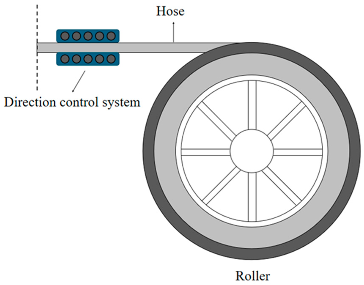
As shown in Figure 5, the system is equipped with a direction and length control system. It automatically adjusts the hose length according to the neural network prediction and feedforward–feedback control strategy to ensure that the hose connection points are always subjected to smooth loading, thereby reducing local wear [41].

Figure 4. Intelligent tensioning system [42].

Figure 4. Intelligent tensioning system [42].

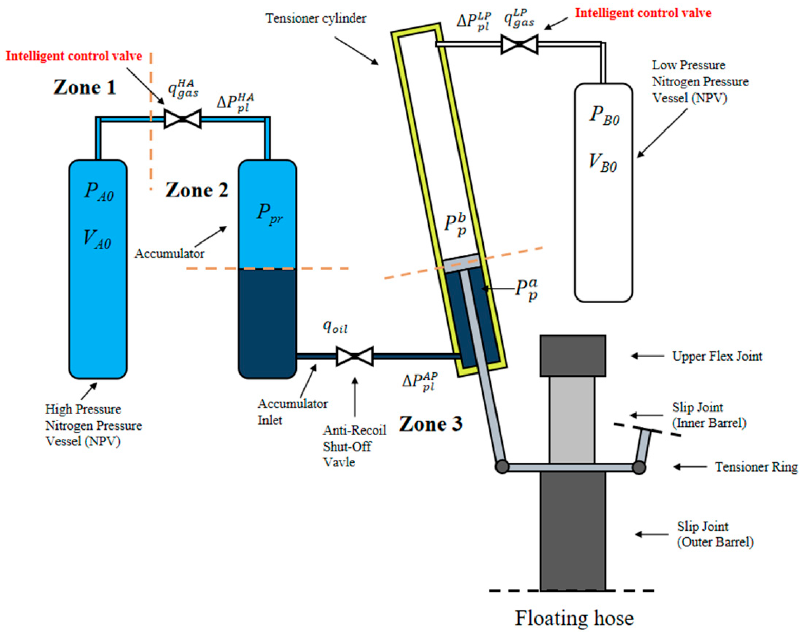
Figure 5. Hose storage and length control system.

Figure 5. Hose storage and length control system.

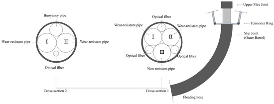
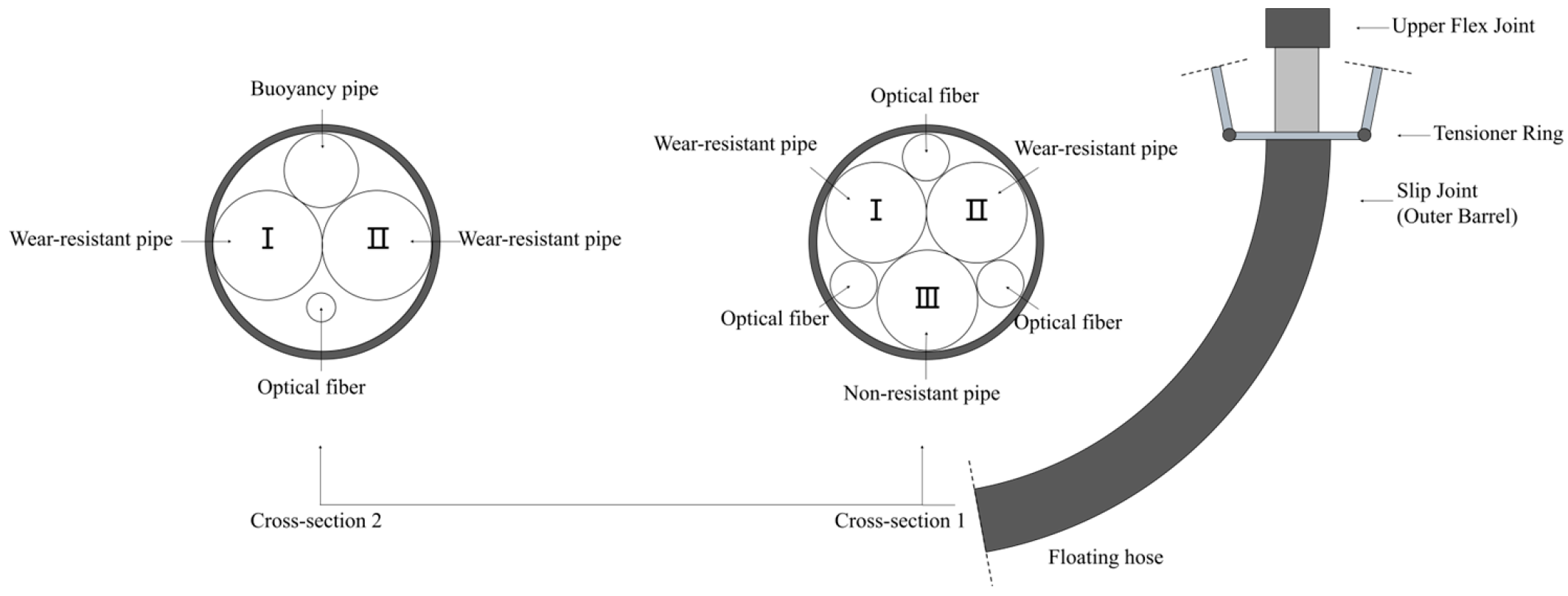
As shown in Figure 6, fiber-optic force measurement is based on the principle of light interference. When the fiber is subjected to external force and undergoes a slight deformation, the light signal (such as wavelength or phase) transmitted within the fiber will change accordingly. By demodulating this change in the light signal, the magnitude and location of the force can be accurately determined. This system is compact, resistant to electromagnetic interference, and is suitable for distributed high-precision force measurement in harsh environments [43]. In this intelligent tensioning system, it is used to detect the tension and curvature of the hose in real time, serving as verification for the prediction results. When the prediction error is significant, fiber optic force measurement data are utilized to adjust the length and direction of the hose to ensure the safety of the operation process.

Figure 6. Intelligent particle flow conveying hose.

2.5. Overall Design Concept

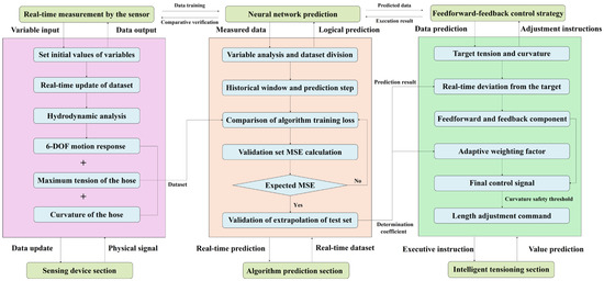
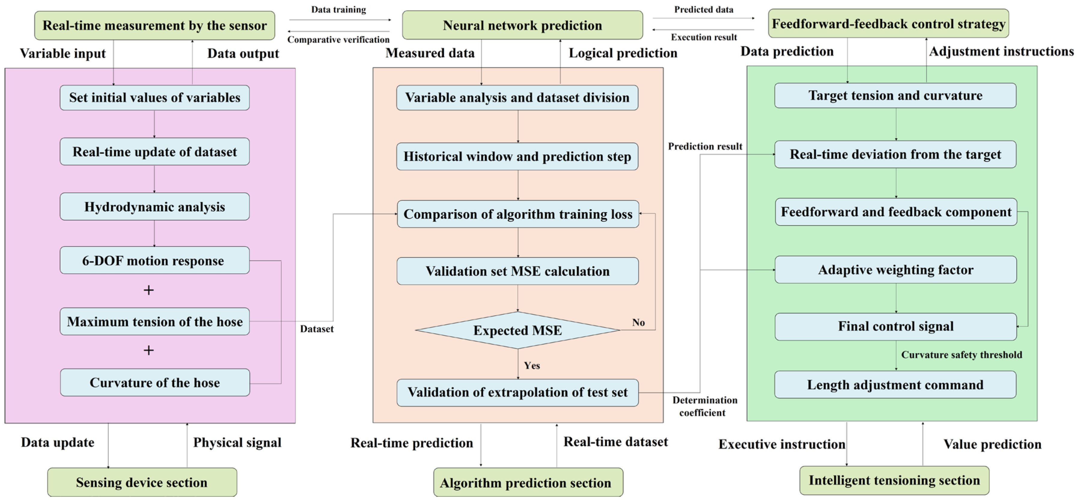
Based on the above theory, an intelligent tensioning system is integrated at the ship, as shown in Figure 7. The 6-DOF motions of the ship are sensed in real time, and the hose tension and curvature are predicted. The feedforward–feedback control strategy then dynamically adjusts the hose length and direction. The hose is consistently maintained in a low-curvature J-shape [44], which ensures stable, efficient and safe transport of solid particles.

Figure 7. Flowchart of the overall design concept.

The proposed system is designed to operate as follows: (1) Real-time 6-DOF motions are acquired from the vessel’s dynamic positioning system or motion reference unit at a sampling rate of 10 Hz. (2) The SA-CNN model, pre-trained on representative sea condition data, predicts the future tension and curvature of the hose with a prediction step size of 5 s. (3) When the predicted curvature exceeds ${\kappa }_{safe}$, an alarm is triggered on the bridge control panel, and the feedforward–feedback controller automatically computes a length adjustment command, $L\left(n\right)$, to shorten the hose. (4) The intelligent tensioning system executes the command through electro-hydraulic servo valves, adjusting the hose length within the physical limits, $L_{\mathrm{m}\mathrm{i}\mathrm{n}}$ and $L_{\mathrm{m}\mathrm{a}\mathrm{x}}$. (5) The entire sensing–prediction–decision–execution loop operates continuously with a cycle time of 0.1 s.

In addition, three key failure modes are considered: (1) Sensor failure: If the 6-DOF motion data are lost, the system falls back to a pure PID feedback mode, relying solely on the tension error signal without feedforward compensation. (2) Communication delay: If the prediction update is delayed beyond 1 s, the system automatically extends the prediction step size from 5 s to 10 s using the most recent available data. (3) Actuator saturation: If the required length adjustment exceeds the physical limits ($L<L_{\mathrm{m}\mathrm{i}\mathrm{n}}$ or $L>L_{\mathrm{m}\mathrm{a}\mathrm{x}}$), the control signal is clipped at the boundary, and a warning is issued to the operator.

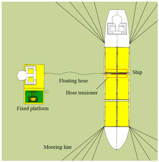
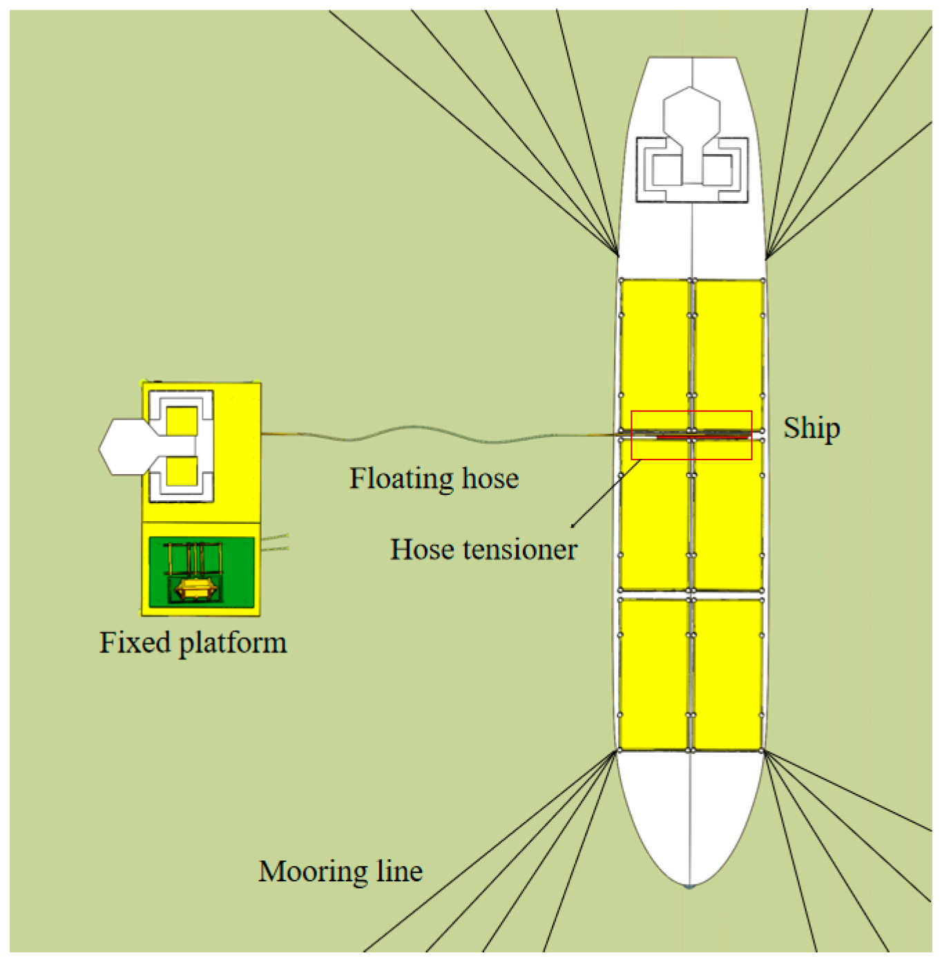
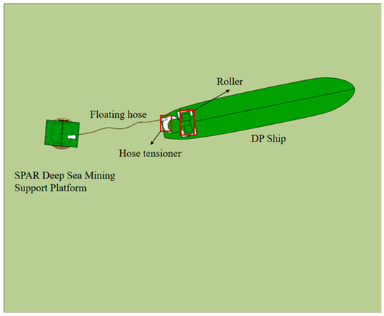
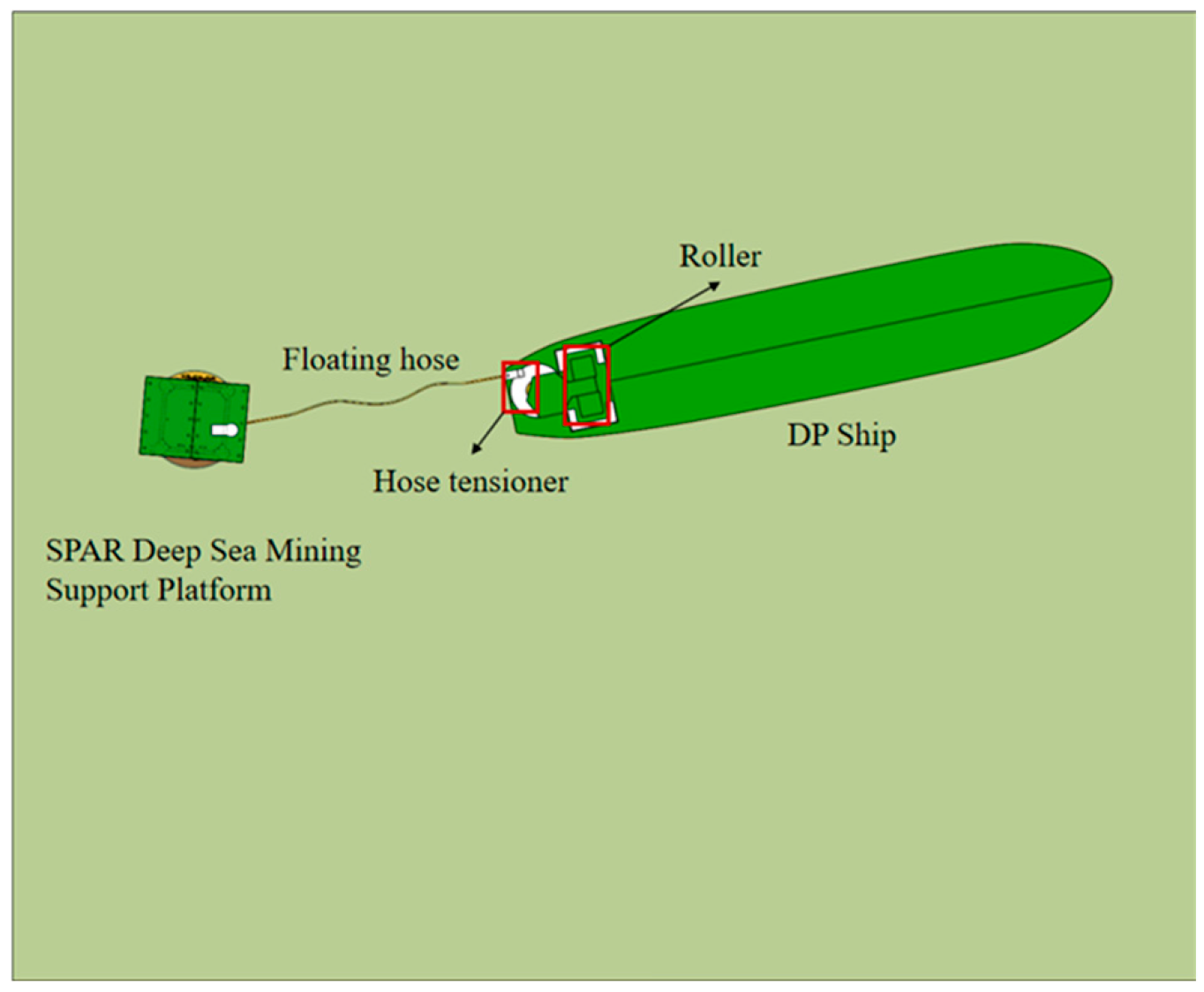
As illustrated in Figure 8 and Figure 9, for offshore resource development, it is necessary to establish a material transfer conduit for platform-to-ship and ship-to-ship operations. In offshore mining, granular flow pipeline connections are required between mining support platforms and solid particle storage vessels [45]. While laying a subsea pipeline via conventional methods would incur substantial engineering costs, directly connecting the fixed platform to the floating production system using a floating hose significantly reduces production expenses [46]. Figure 8 depicts an offshore scene using a multi-point moored ship and a fixed platform. Figure 9 depicts a deep-sea scene using a dynamic positioning (DP) ship and a floating platform.

Figure 8. Permanent floating hose transfer system between offshore multi-point mooring ship and fixed platform.

Figure 9. Permanent flexible solid transfer system between DP ship and floating platform.

Based on the above concept, three design criteria are established for the control system.

(1)

Curvature constraint: To prevent particle deposition in granular flow, the ratio of curvature radius, $R$, to pipe diameter, $D$, must satisfy [47]

$$R/D>4,$$

(26)

where $R=1/\kappa$ represents the radius of the curvature, and $D$ represents the pipe diameter. For $D=0.6 \mathrm{m}$, this design criterion gives $R=5 \mathrm{m}$, so ${\kappa }_{safe}=0.2 {\mathrm{m}}^{-1}$.

(2)

Tension constraint: To avoid excessive stretching, the maximum tension must be maintained within 60% [48] of the material’s ultimate tension, $T_{ult}$

$$T\le T_{max}=0.6·T_{ult},$$

(27)

where $T_{max}$ represents the maximum allowable tension, and $T_{ult}$ represents the ultimate tensile strength.

(3)

Dual-objective safety domain: The system must maintain the hose state within a safe operating region defined by both tension and curvature bounds

$$S=\left[\right(T,\kappa \left)\right|T\le T_{max},\kappa \le {\kappa }_{max}],$$

(28)

where $S$ represents the safe operating region of the hose.

3. Numerical Simulation

3.1. Oceanographic Parameters

This study assumes that the wave and current directions are consistent, and that the angle between the wind direction and the wave–current direction is 45°. The other angles are shown in Section 4.5. The wave spectrum is taken to be the JONSWAP spectrum [49]. Second-order wave drift forces are neglected. The sea conditions are once in a year, once in a century and once in a thousand years from realistic offshore metocean datasets. The relevant parameters are shown in Table 1.

Table 1. Sea state parameters.

Sea Condition	Wave Parameter			Current Parameter			Wind Parameter
	Significant Wave Height (m)	Peak Period (s)	Peak Enhancement Factor	Flow Velocity (m/s)			Average Wind Speed (m/s)
	Hs	Tp	γ	0 m	10 m	20 m	30 m	45°
Once in a year	4.52	9.45	1.89	1.24	1.07	0.83	0.53	24
Once in a century	13.7	15.1	2.4	2.49	2.14	1.67	1.07	45.1
Once in a thousand years	16.5	15.9	2.75	2.76	2.37	1.85	1.23	50.9

3.2. Simulation Results

The system is simulated for 10,800 s (3 h) in OrcaFlex (version 11.0), coupling environmental loads (wind, waves and currents) under three sea states (once in a year, once in a century, and once in a thousand years) with three hose lengths (145 m, 150 m, and 155 m). The hose is modeled as a slender beam–column structure using the lumped-mass method implemented in OrcaFlex, with boundary conditions including the fixed connection at the platform side and the fixed connection at the vessel side. This study assumes that the results obtained from the numerical simulation software are correct [50]. The tension and curvature at each point under different hose lengths are solved.

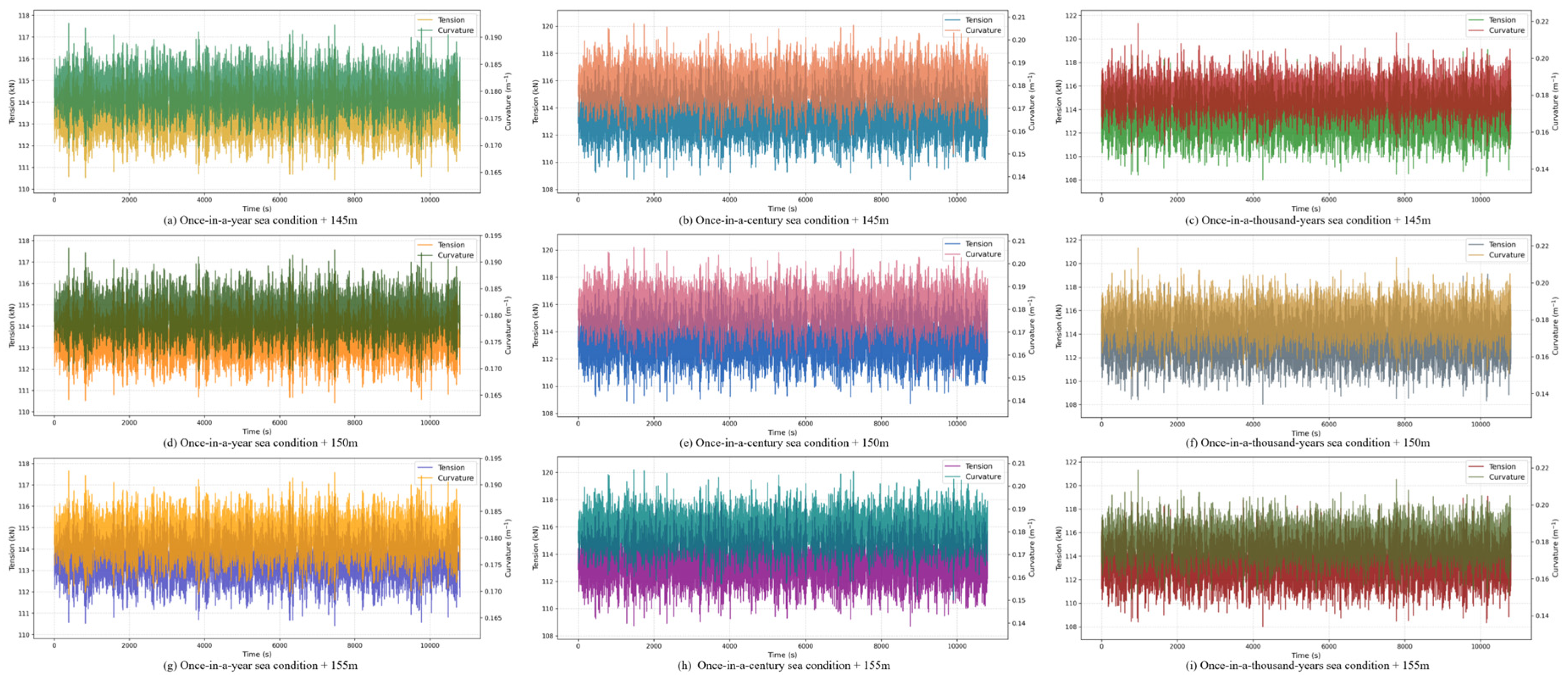
As shown in Figure 10, under nine different operating conditions, the tension and curvature of the hose both meet the design requirements as described in Section 2.5 [51]. As the sea conditions deteriorate, the tension and curvature of the hose increase, while the safety redundancy decreases. As the length of the hose changes, the tension and curvature do not change significantly. Therefore, it is reasonable to select operating conditions combining the once-in-a-year and once-in-a-century sea states with hose lengths of 145 m and 150 m as the training set, while the remaining conditions are used as the test set.

Figure 10. Hose tension and curvature under different operating conditions. (a) Once-in-a-year sea condition + 145 m; (b) once-in-a-century sea condition + 145 m; (c) once-in-a-thousand-years sea condition + 145 m; (d) once-in-a-year sea condition + 150 m; (e) once-in-a-century sea condition + 150 m; (f) once-in-a-thousand-years sea condition + 150 m; (g) once-in-a-year sea condition + 155 m; (h) once-in-a-century sea condition + 155 m; (i) once-in-a-thousand-years sea condition + 155 m.

The 6-DOF motions of the ship will significantly affect the tension and curvature of the hose, thereby impacting the safety of the system. In DP ships, the 6-DOF motions are controlled by GPS and their own power systems [52]. In multi-point mooring ships, 6-DOF motions of ships are related to the design of the mooring system. This study investigates the relationship between mooring line length and hose tension and curvature under the once-in-a-thousand-years sea condition with a hose length of 145 m.

As shown in Table 2, the longer the mooring line is, the greater the hose tension, the greater the curvature and the greater the ship’s movement distance. The shorter the mooring line is, the smaller the hose tension, the smaller the curvature and the smaller the ship’s movement distance. Taking into account the safety of mooring, as well as the requirements for hose tension and curvature [53], the final length of the mooring lines is determined to be 93 m.

Table 2. Simulation of different mooring line lengths.

Mooring Line Length (m)	Maximum Tension (kN)	Maximum Curvature (m−1)	Maximum Movement Distance of the Ship (m)
93	119.10	0.2189	14.47
94	119.14	0.2189	16.01
95	119.15	0.2291	17.53
96	119.19	0.2292	19.18
97	119.21	0.2294	20.62

3.3. Dataset Establishment

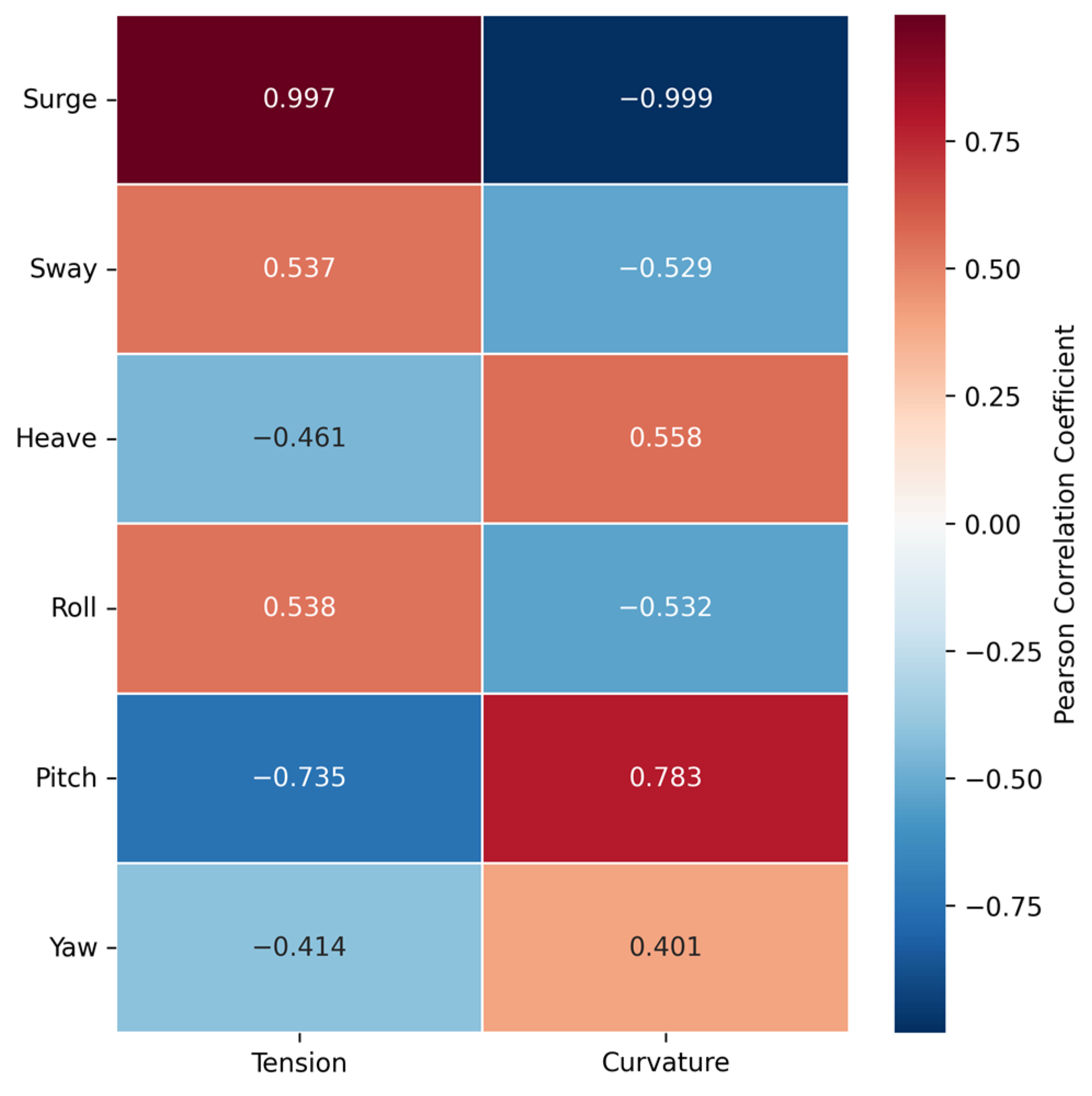
To quantitatively evaluate the linear explanatory power of the ship’s 6-DOF motion components for the tension and curvature of the hose, this study calculates the Pearson correlation coefficient [54] between the independent variables and the dependent variables.

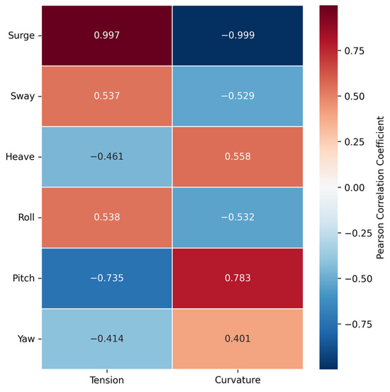
As shown in Figure 11, the correlation coefficients between surge and tension and between surge and curvature are 0.997 and −0.999, respectively, indicating a near-linear relationship [55]. This indicates that within the analyzed operating conditions, the X-axis displacement of the floating platform is the most significant motion component determining the changes in hose tension and curvature. The correlation coefficients between yaw and tension, and yaw and curvature are −0.414 and 0.401 respectively. Among the six motion components, they are the lowest. This is because yaw mainly causes the platform to rotate around the Z-axis, and its contribution to the changes in hose tension and curvature is relatively limited [56]. The above correlation analysis results indicate that there is a strong linear correlation structure between the 6-DOF motions of the ship and the mooring tension and curvature. Moreover, whether a DP ship or a multi-point moored ship is considered, its 6-DOF motions can be easily measured. Therefore, it is reasonable to use the 6-DOF motions of the ship as independent variables and the corresponding hose maximum curvatures and maximum tensions as dependent variables.

Figure 11. Data correlation heatmap.

To ensure the temporal sequence of the data [57], this study does not shuffle the data and divides the data in sequence. At the same time, to avoid the problem of non-independence of samples caused by high-frequency sampling [58], this study uses a sampling frequency of 10 Hz. As shown in Table 3, to make full use of the database, in this study, the data with hose lengths of 145 m and 150 m under the once-in-a-year and once-in-a-century sea conditions are classified as Class A. The hose length of 155 m and sea condition of once in a thousand years are classified as Class B. The first 70% of the Class A data are used for model training, and the next 15% are used for evaluating the loss function [59], while the remaining 15% are used for model generalization evaluation along with the Class B data.

Table 3. Database partitioning.

Parameters	145 m	150 m	155 m
Once in a year	Class A	Class A	Class B
Once in a century	Class A	Class A	Class B
Once in a thousand years	Class B	Class B	Class B

The training set does not use all the data from Class A, in order to prevent overfitting and to enhance its generalization ability [60]. The validation set utilizes the next 15% of Class A, mainly for evaluating the loss function. The test set uses the last 15% of Class A and all the Class B data, ensuring that the models have never seen these data during training [61]. This was done to verify the generalization ability of the model.

4. Neural Network Prediction

This study compares the training performance of Model-I (RNN), Model-II (LSTM), Model-III (CNN) and Model-IV (SA-CNN) under different historical window lengths and prediction step sizes. Meanwhile, this study examines the predictive performance of four models under different sea conditions and hose lengths and compares the generalization capabilities of the four models.

4.1. Training Process

In this study, the training parameters of four models are shown in Table 4. The detailed configuration of Model-IV is shown in Table 5. Each model includes early stopping [62] based on the validation loss, with a patience of 50 epochs to prevent overfitting.

Table 4. The training parameters of four models.

Model	Batch Size	Initial Learning Rate	Weight Decay	Early Stopping Patience	Activation Function	Dropout
Model-I	128	1 × 10−3	1 × 10−5	50	tanh	0.3
Model-II	128	1 × 10−3	1 × 10−5	50	tanh/ReLU	0.3
Model-III	128	1 × 10−3	1 × 10−5	50	ReLU	0.3
Model-IV	128	1 × 10−3	1 × 10−5	50	ReLU	0.3

Table 5. The detailed configuration of Model-IV.

Layer	Configuration
Input	Shape		(batch, channels, historical window length) = (batch, 6, H)
Feature extraction backbone (CNN)	Conv1D layer 1	Filters	32
		Kernel size	3
	MaxPooling1D	Pool size	2
		Stride	2
	Conv1D layer 2	Filters	64
		Kernel size	3
	MaxPooling1D	Pool size	2
		Stride	2
	Conv1D layer 3	Filters	128
		Kernel size	3
	MaxPooling1D	Pool size	2
		Stride	2
Spatial attention module	Input to attention		(batch, 128, 1, H/8)—unsqueezed to add height dimension for 2D convolution
	2D Convolution	Filters	1
		Kernel size	3 × 3
	Element-wise product		(batch, 128, H/8)
Fully connected layers	Dense layer 1	Number of neurons	64
	Dense layer 2 (output)	Number of neurons	2 (predicted tension and curvature)
Total trainable parameters	Approximately 80,885 (H = 50)

The temporal dynamics are handled by a sliding historical window and prediction step size. The historical window length and prediction step size used in this study are shown in Table 6. Historical window length (H) represents the number of seconds of the past data used for training. Prediction step size (P) represents the number of seconds ahead for which the tension and curvature are to be predicted.

Table 6. Different combinations of historical window length and prediction step size.

Parameters	Prediction Step Size, 5 s	Prediction Step Size, 10 s	Prediction Step Size, 20 s
Historical window length, 5 s	H5P5	H5P10	H5P20
Historical window length, 10 s	H10P5	H10P10	H10P20
Historical window length, 20 s	H20P5	H20P10	H20P20

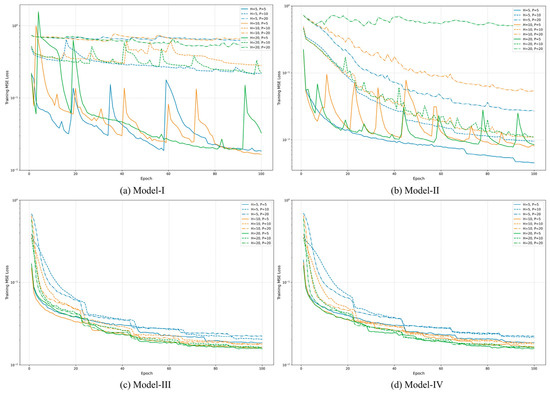
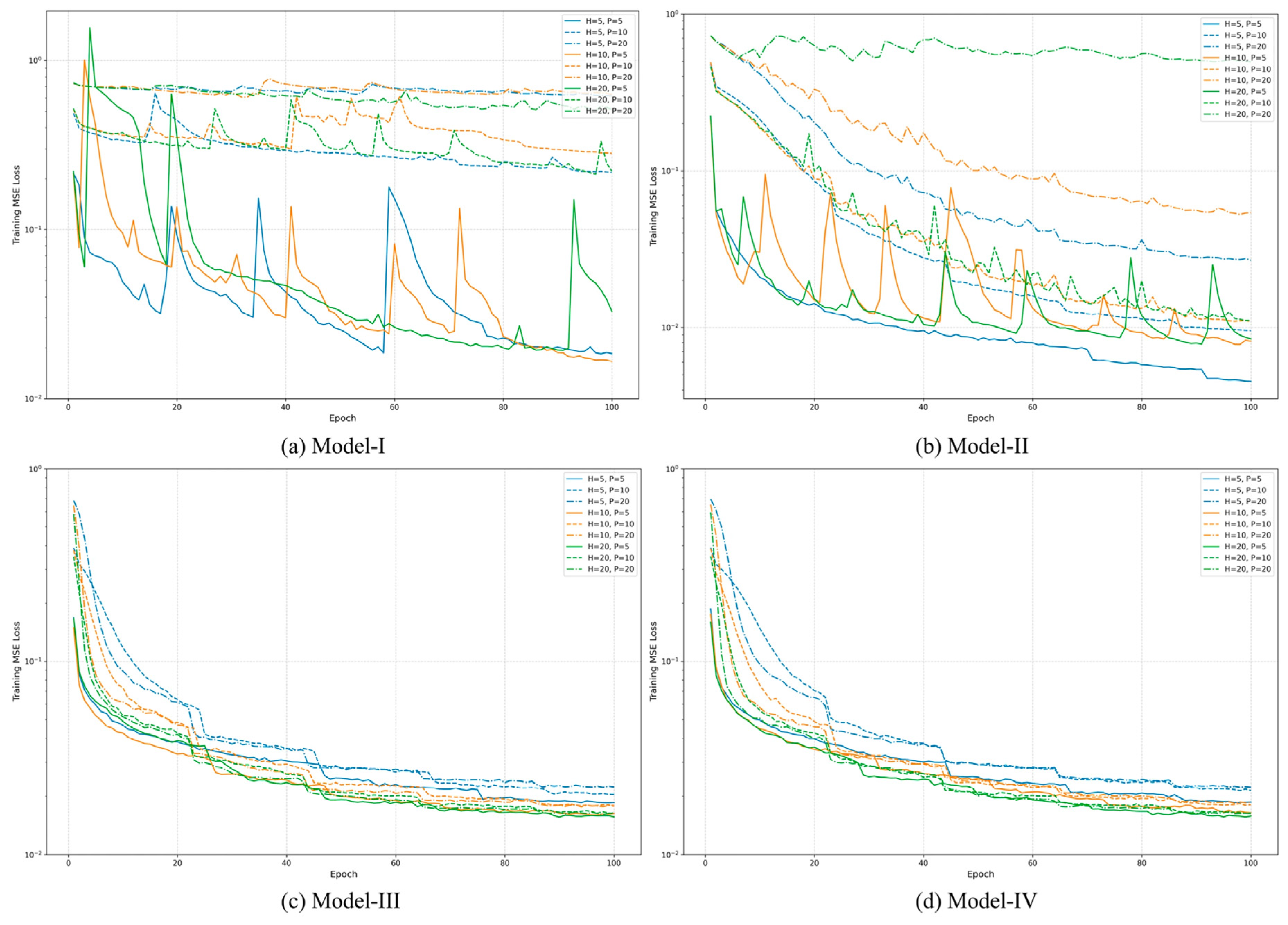
The training process of the first 100 epochs is shown in Figure 12. It is worth noting that the model outputs tension and curvature, so there are two MSE loss values. However, to facilitate an evaluation of the model performance, in the model evaluation part of this study, the average MSE loss is used as the loss function, and the two loss values will be separately presented in the subsequent prediction part. Among the 9 combinations of historical window length and prediction step size, the H20P5 combination shows a faster decrease and a smaller final stable loss value; the H5P20 combination shows a slower decrease and a larger final stable loss value. This indicates that the combination of a longer historical window length and a shorter prediction step size reduces learning complexity, while the opposite combination increases it [63]. This characteristic is the same for all four models. However, the training error curves of Model-III and Model-IV exhibit a more stable and faster decline, and their final stable loss values are smaller. The training error curves of Model-I and Model-II fluctuate more significantly, and the final stable loss function value is larger, but they still show a downward trend. From this, it can be seen that Model-III and Model-IV are more suitable for this study compared to Model-I and Model-II.

Figure 12. Loss function (average MSE loss) during the training process of different neural network models. (a) Model-I; (b) Model-II; (c) Model-III; (d) Model-IV.

4.2. Hyperparameter Optimization

Based on the models trained with the 9 different historical window lengths and prediction step sizes mentioned above, this study uses the test set of Class A to optimize the hyperparameters. Four models respectively use 9 sets of hyperparameters to predict the hose tension and curvature and compare them with the actual values, calculating their average R² scores.

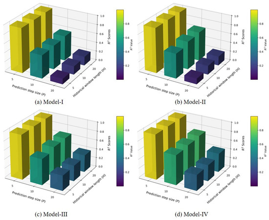
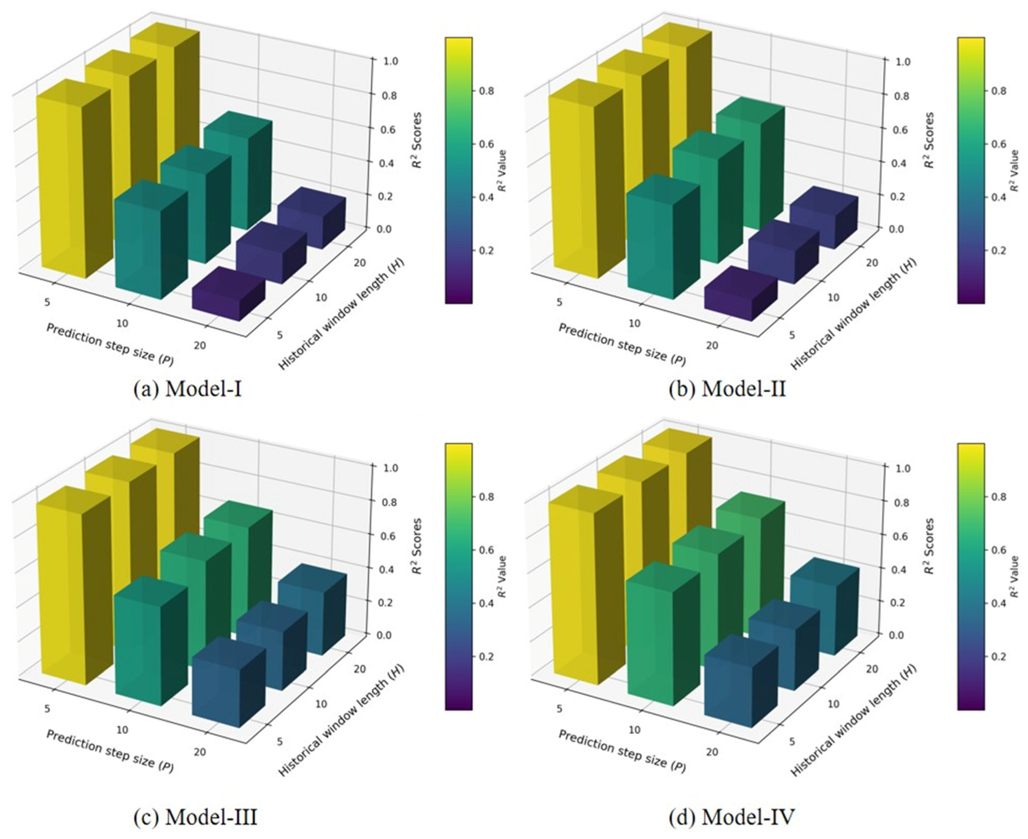
As shown in Figure 13 and Table 7, for all historical window lengths, increasing the prediction step size significantly decreases the R² scores of each model. Taking H = 20 s as an example, when P increases from 5 s to 20 s, the R² score of SA-CNN drops sharply from 0.9965 to 0.4145, a decrease of 58.4%. This phenomenon indicates that the dynamic evolution of the hose has a strong short-term correlation. As the prediction time scale increases, the system state uncertainty accumulates, which fundamentally constrains the extrapolation ability of data-driven models [17].

Figure 13. Average R² scores for four models with nine hyperparameters. (a) Model-I; (b) Model-II; (c) Model-III; (d) Model-IV.

Table 7. Average R² scores of four models with nine hyperparameters.

Parameters	Model Type	Prediction Step Size, 5 s	Prediction Step Size, 10 s	Prediction Step Size, 20 s
Historical window length, 5 s	Model-I	0.9839	0.5097	0.1201
	Model-II	0.9875	0.5455	0.1242
	Model-III	0.9819	0.5701	0.3318
	Model-IV	0.9900	0.6541	0.3461
Historical window length, 10 s	Model-I	0.9874	0.5267	0.1828
	Model-II	0.9916	0.6158	0.1953
	Model-III	0.9920	0.6395	0.3431
	Model-IV	0.9953	0.6835	0.3555
Historical window length, 20 s	Model-I	0.9892	0.5525	0.1964
	Model-II	0.9922	0.6393	0.2021
	Model-III	0.9934	0.6544	0.3763
	Model-IV	0.9965	0.7096	0.4145

Increasing the historical window length generally improves the prediction accuracy, but the improvement rate decreases as the historical window length increases. Taking SA-CNN with p = 10 s as an example, when H increases from 5 s to 10 s, the R² score increases from 0.6541 to 0.6835 (a relative increase of 4.5%); further increasing to 20 s yields an R² score of 0.7096 (only a 3.8% relative increase). This indicates that the main dynamic characteristics of the hose response can be captured by historical motion information within the range of 5 s to 10 s. Although an excessively long historical window length can provide additional context, the ratio of computational cost to accuracy gain gradually decreases.

Model-IV achieves the highest R² scores in all 9 hyperparameter combinations. Especially at the short prediction step size (p = 5 s), its R² score remains above 0.99, almost achieving a perfect fit for the mooring tension. This clearly indicates that Model-IV is suitable for this study.

As mentioned above, a longer historical window length can improve the model’s accuracy, but the training process becomes more unstable. A shorter prediction step size can significantly reduce the error, but the model can predict for a shorter time interval [22]. This study strikes a balance between accuracy and prediction time interval, ultimately selecting the H10P5 combination for the subsequent analysis.

4.3. Training Results

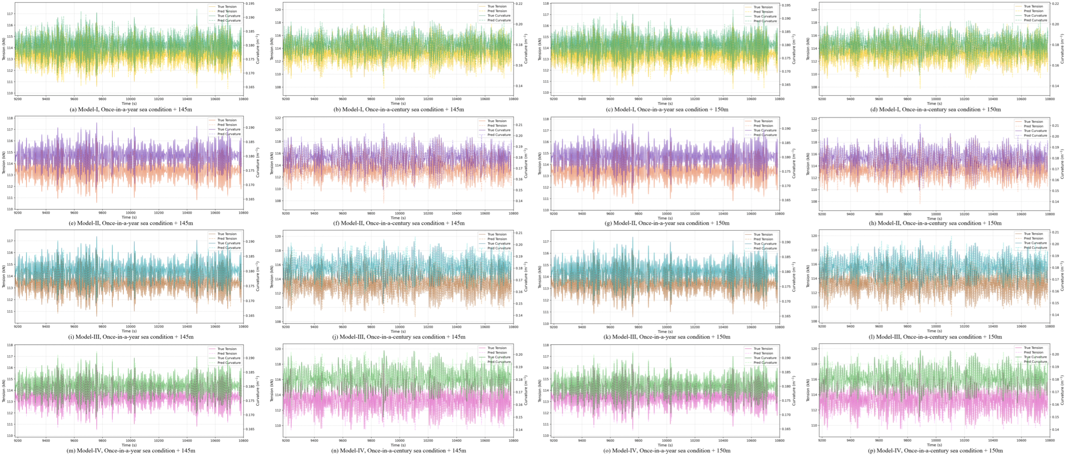
Using the model optimized with the above hyperparameters, predictions are made for the test set data of four combinations of operating conditions (two environmental conditions: once in a year and once in a century; two hose lengths: 145 m and 150 m). The dataset includes data not encountered by the models during training under the same operating conditions. The predicted values are compared with the actual values. As shown in Figure 14, the predictions for hose tension and curvature are plotted on the same graph, distinguished by different colors. The solid line represents the actual values, and the dashed line represents the predicted values. It can be seen that the dashed line and the solid line are basically overlapping, indicating that each model performs well, makes accurate predictions, and precisely captures the relationship between the independent variable and the dependent variable.

Figure 14. R² scores of four models on test set with different operating conditions. (a) Model-I, once-in-a-year sea condition + 145 m; (b) Model-I, once-in-a-century sea condition + 145 m; (c) Model-I, once-in-a-year sea condition + 150 m; (d) Model-I, once-in-a-century sea condition + 150 m; (e) Model- II, once-in-a-year sea condition + 145 m; (f) Model-II, once-in-a-century sea condition + 145 m; (g) Model-II, once-in-a-year sea condition + 150 m; (h) Model-II, once-in-a-century sea condition + 150 m; (i) Model-III, once-in-a-year sea condition + 145 m; (j) Model-III, once-in-a-century sea condition + 145 m; (k) Model-III, once-in-a-year sea condition + 150 m; (l) Model-III, once-in-a-century sea condition + 150 m; (m) Model-IV, once-in-a-year sea condition + 145 m; (n) Model-IV, once-in-a-century sea condition + 145 m; (o) Model-IV, once-in-a-year sea condition + 150 m; (p) Model-IV, once-in-a-century sea condition + 150 m.

To quantitatively evaluate the predictive accuracy of the four models, this study calculates the R² scores, RMSE and MAE between the predicted and true values for each model on the test set.

As shown in Table 8, under all four operating conditions, Model-IV achieves the highest R² scores (all greater than 0.97) and the lowest RMSE in all cases, indicating its outstanding time series feature extraction ability and generalization performance. Taking the once-in-a-year sea condition and 145 m hose length as an example, the R² score of Model-IV reaches 0.9922, which is 16.9% higher than that of Model-I, 5.6% higher than that of Model-II and 4.9% higher than that of Model-III. The introduction of the spatial attention mechanism in Model-IV enables the model to dynamically focus on the key time positions in the input features that are highly related to hose tension and curvature, thereby maintaining excellent predictive ability in various environments.

Table 8. R² scores, RMSE and MAE of four models with different operating conditions.

Models	Model-I			Model-II			Model-III			Model-IV
	R2-Scores	RMSE	MAE	R2-Scores	RMSE	MAE	R2-Scores	RMSE	MAE	R2-Scores	RMSE	MAE
1 year + 145 m	0.8489	0.8383	0.8236	0.9396	0.7369	0.7187	0.9456	0.7015	0.6879	0.9922	0.6925	0.6778
100 years + 145 m	0.8022	0.8804	0.8623	0.8708	0.7488	0.7364	0.9335	0.7273	0.7165	0.9834	0.6934	0.6851
1 year + 150 m	0.8497	0.8884	0.8707	0.9222	0.7248	0.7098	0.9502	0.7006	0.6954	0.9958	0.6920	0.6774
100 years + 150 m	0.8011	0.8884	0.8827	0.8712	0.7571	0.7388	0.9324	0.7400	0.7327	0.9723	0.6949	0.6836

When the sea condition changes from once in a year to once in a century, the performance of all models deteriorates to varying degrees. In particular, the R² scores of Model-I and Model-II decrease significantly, and their RMSE values increase markedly. This suggests that the mapping capacity of the recurrent architectures (Model-I and Model-II) is insufficient under different sea conditions, making it difficult to accurately capture the complex coupling between ship motion and hose response. However, varying the hose length has almost no impact on the performance of the four models.

From this, it can be seen that for the test set data of the four combinations of operating conditions, all four models have varying degrees of generalization ability [23]. Among them, Model-IV performs the best and has the potential to be deployed in an actual hose monitoring system.

4.4. Verification of the Extrapolation Ability of the Model

In actual engineering, operating conditions are highly complex and variable. Therefore, it is necessary to evaluate the performance of the model under extreme operating conditions [24]. This section evaluates the performance of the four models under the extreme condition of the once-in-a-thousand-years sea state with a hose length of 155 m in Class B and compares their generalization capabilities.

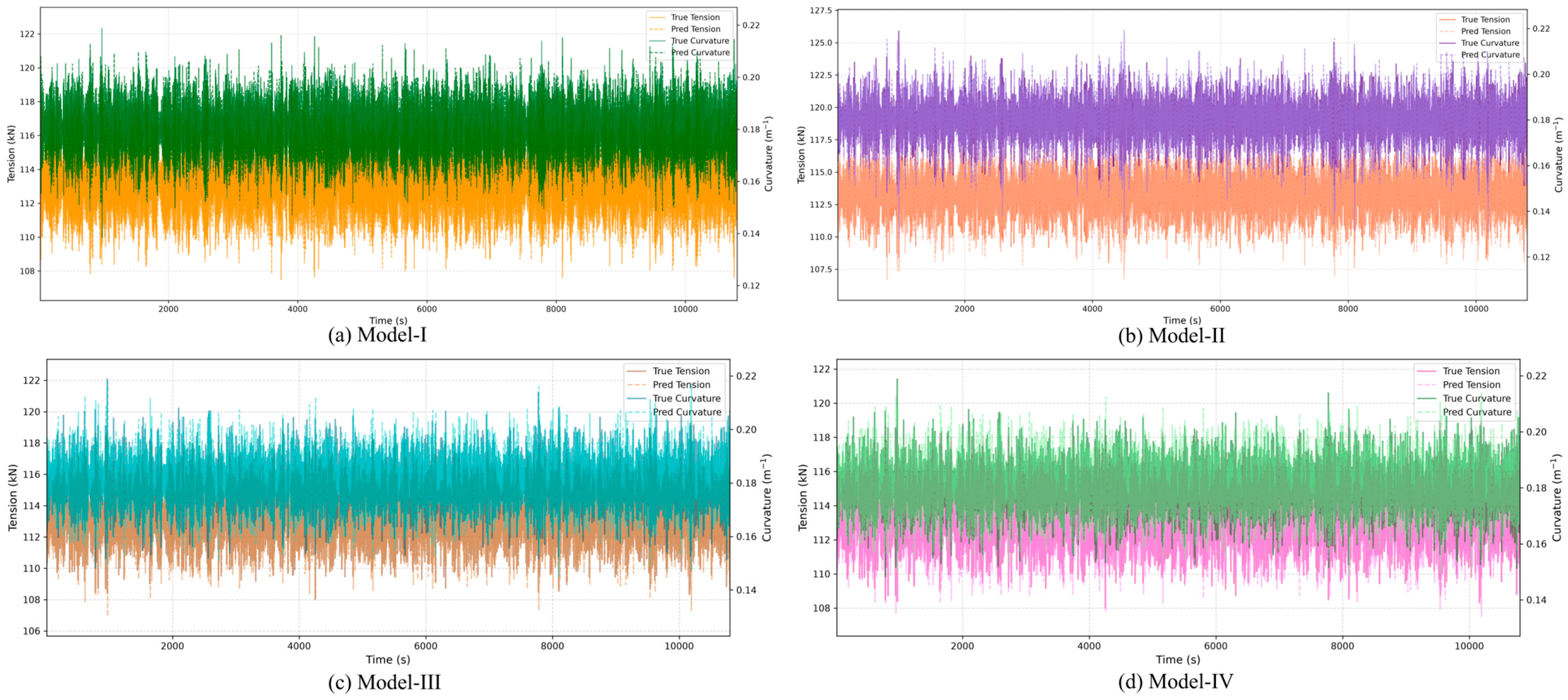
As shown in Figure 15, under extreme operating conditions, the predicted values of the four models are in close agreement with the true values. This indicates that the four models have achieved good predictive results, successfully forecasting the overall trends and major fluctuations of hose tension and curvature. This also proves that all four models possess varying degrees of generalization ability.

Figure 15. Prediction results of four models on test set under extreme operating conditions. (a) Model-I; (b) Model-II; (c) Model-III; (d) Model-IV.

To quantitatively evaluate the predictive accuracy of the four models, this part also calculates the R² scores, RMSE and MAE of the predicted values and true values for each model under extreme operating conditions.

As shown in Table 9, when the model encounters unknown sea conditions, the prediction accuracy decreases. Taking Model-IV as an example, the R² score drops from 0.9723 (100 years + 150 m operating condition) to 0.8737 (1000 years + 155 m operating condition), a decrease of 10.1%, and RMSE increases from 0.6949 to 0.7480. The degradation of Model-I is even more severe; its R² score has fallen to 0.7061, and its RMSE soars to 1.0731, an increase of more than 25% compared to the 1 year + 145 m operating condition. Although the overall performance declines, Model-IV still maintains relatively good prediction performance with an R² score of 0.8737. Thus, it retains good predictive ability even under extreme operating conditions.

Table 9. R² scores, RMSE and MAE of four models under extreme operating conditions.

Models	Model-I			Model-II			Model-III			Model-IV
	R2-Scores	RMSE	MAE	R2-Scores	RMSE	MAE	R2-Scores	RMSE	MAE	R2-Scores	RMSE	MAE
1000 years + 155 m	0.7061	1.0731	1.0333	0.7717	0.9361	0.9156	0.8171	0.8730	0.8561	0.8737	0.7480	0.7197

4.5. Generalization Ability of Wind, Wave and Current Directions

This section investigates the prediction performance of the model under different wind, wave and current directions, thereby demonstrating its applicability in real engineering [64]. It should be noted that in this section, the operating condition is assumed to be the once-in-a-year sea state with a hose length of 145 m. At the same time, this section assumes that the wave and the current are in the same direction. Theoretically, the relationship between the independent variables and the dependent variables learned by the model is independent of the environmental load direction. Therefore, this study hypothesizes that the model’s prediction accuracy is independent of the angle. The model still maintains good prediction performance under different angles.

As shown in Table 10, under different wind and wave–current angle conditions, the variations in R² scores, RMSE and MAE for each model do not show significant differences. Furthermore, among all the wind and wave–current angles, Model-IV achieves the highest R² scores and the lowest RMSE and MAE, indicating that this model has the strongest generalization ability for the location’s operating conditions. These results demonstrate the generalization ability of each model with respect to the directions of wind, waves and currents [65].

Table 10. R² scores, RMSE and MAE of four models with different angles of wind and wave–current.

Models	Model-I			Model-II			Model-III			Model-IV
	R2 Scores	RMSE	MAE	R2-Scores	RMSE	MAE	R2-Scores	RMSE	MAE	R2-Scores	RMSE	MAE
0°	0.8049	0.8659	0.8596	0.9465	0.7228	0.7218	0.9571	0.6985	0.6735	0.9921	0.6929	0.6732
15°	0.7945	0.8686	0.8495	0.9345	0.7392	0.7278	0.9347	0.7158	0.6841	0.9845	0.6974	0.6781
30°	0.8446	0.8413	0.8362	0.9245	0.7449	0.7341	0.9435	0.7041	0.6712	0.9738	0.7059	0.6698
45°	0.8489	0.8383	0.8197	0.9396	0.7369	0.7235	0.9456	0.7015	0.6785	0.9922	0.6925	0.6731
60°	0.8254	0.8573	0.8462	0.9372	0.7383	0.7105	0.9554	0.6987	0.6982	0.9842	0.6994	0.6824
75°	0.8475	0.8398	0.8275	0.9127	0.7584	0.7437	0.9345	0.7162	0.6941	0.9754	0.7015	0.6812
90°	0.8515	0.8365	0.8261	0.9416	0.7237	0.7068	0.9454	0.7034	0.6854	0.9987	0.6902	0.6442

5. Intelligent Control Performance Verification

This study proposes a feedforward–feedback control strategy to generate the length adjustment command. The feedforward component is derived from neural network predictions, and the feedback component is provided by PID control.

5.1. Feasibility Analysis of Intelligent Tensioning System

Based on the above neural network analysis results, SA-CNN achieves the highest R² scores in all 9 combinations of hyperparameters and all operating conditions. Therefore, in this study, this model is selected as the core prediction model for the intelligent tensioning system. By sensing the 6-DOF motions of the ship, the SA-CNN model predicts the future tension and curvature of the hose and then drives the feedforward–feedback controller to regulate the hose based on the difference between the target values and the predicted values.

As shown in Table 11, the curvature and tension of the hose vary with hose length. The longer the hose is, the greater the curvature and the lower the tension [44]. When the neural network predicts an excessive curvature of the hose, the intelligent tensioning system shortens the hose length using the feedforward–feedback control strategy. This demonstrates the feasibility of using an intelligent tensioning system to adjust the hose length and keep the tension and curvature within a reasonable range. As long as the accuracy and generalization of the neural network prediction model are ensured, the system can theoretically guarantee continuous and reliable hose transportation under different sea conditions.

Table 11. The maximum tension and curvature of the hose under different hose lengths and sea conditions.

Parameters	145 m		150 m		155 m
	Curvature (m−1)	Tension (kN)	Curvature (m−1)	Tension (kN)	Curvature (m−1)	Tension (kN)
Once in a year	0.1926	116.43	0.1928	116.41	0.1929	116.35
Once in a century	0.2073	118.28	0.2076	118.25	0.2081	118.15
Once in a thousand years	0.2189	119.10	0.2186	119.08	0.2182	119.01

5.2. Simulation Setup and Evaluation Metrics

To validate the effectiveness of the proposed composite control strategy, a numerical simulation platform was developed in MATLAB (version R2025a). The simulation platform consists of three modules: (1) an SA-CNN predictor trained on the dataset, which provides feedforward predictions of hose tension and curvature; (2) a PID controller [35] with feedforward compensation; and (3) a superposition scheme that the applies feedforward–feedback strategy.

The intelligent control performance verification is performed using the tension and curvature time series data under the once-in-a-year sea condition with the hose length of 145 m. The dataset contains 10,800 s of data sampled at 10 Hz. The tension and curvature responses of the hose under this operating condition serve as the open-loop baseline [66]. The SA-CNN predictions of tension and curvature are pre-computed. At each time step, the controller computes the required length adjustment, $L\left(n\right)$. The control effect, $K_T·L\left(n\right)$, is then directly superimposed on the tension response to obtain the controlled tension.

The superposition-based approach adopted in this study is a common preliminary validation method for control algorithms in offshore engineering, as it allows for rapid assessment of control effectiveness without the computational burden of fully coupled simulations. However, it should be noted that this method neglects the feedback coupling between the hose dynamics and the control action. Therefore, the quantitative results are indicative of the control potential rather than the actual closed-loop performance. The primary contribution of this section is to demonstrate that the feedforward component derived from SA-CNN predictions can effectively suppress the oscillations introduced by pure PID feedback, as shown by the comparative analysis.

Three control strategies are implemented and compared under the same operating condition.

Case 1 is an open-loop scenario, which serves as the baseline. The hose length is fixed, and no active control is applied.

Case 2 is a pure PID feedback controller, where only the feedback component of the controller is active. The control signal is computed as

$$L\left(n\right)=-0.5·u_T\left(n\right),$$

(29)

where $L\left(n\right)$ represents the control signal, and $u_T\left(n\right)$ represents the PID output based on the tension prediction error. The PID gains are tuned using the Ziegler–Nichols method [67] and refined manually for the hose-tension control application. Finally, $K_p=1.0$, $K_i=0.5$, and $K_d=0.05$ [68].

Case 3 is the composite feedforward–feedback control proposed in this study. The feedforward component is computed from SA-CNN predictions

$$L_{ff}\left(n\right)=-0.3·K_{ff}·(\widehat{T}\left(n+p\right)-T_{target}),$$

(30)

where $L_{ff}\left(n\right)$ represents the feedforward component, $K_{ff}$ represents the feedforward coefficient, $p=50$ steps (5 s), $\widehat{T}$ represents the SA-CNN tension prediction, and $T_{target}=113 \mathrm{k}\mathrm{N}$ represents the target tension. The feedback component is the same PID controller as in Case 2. The final control action is a weighted combination

$$L\left(n\right)=\lambda ·L_{ff}\left(n\right)+\left(1-\lambda \right)·L_{fb}\left(n\right),$$

(31)

where $\lambda$ represents the adaptive weight based on the prediction accuracy, and $L_{fb}\left(n\right)$ represents the feedback component. Owing to the high prediction accuracy of SA-CNN, the model prediction error remains below 5% in the vast majority of operating conditions. Consequently, the adaptive weight, $\lambda$, maintains a relatively large value, and the control action relies primarily on the feedforward contribution. Only in rare cases where the prediction error unexpectedly exceeds 5% does $\lambda$ automatically reduce the feedforward contribution, shifting greater reliance to PID feedback.

It is worth noting that tension is chosen as the primary control target because the length adjustment operation has opposite physical effects on tension and curvature; they cannot both be used as control targets simultaneously [26]. Tension directly determines the structural integrity and fatigue life of the floating hose, while curvature serves only as a safety constraint. When the curvature exceeds ${\kappa }_{safe}=0.2 {\mathrm{m}}^{-1}$, the control action is automatically attenuated by a decay factor

$$d=\max \left(\mathrm{0.3,1}-{\displaystyle \frac{\kappa -{\kappa }_{safe}}{0.05}}\right).$$

(32)

This mechanism prevents the hose from excessive bending while maintaining tension control. To quantitatively evaluate the control performance, a peak reduction ratio is adopted

$$R_{peak}={\displaystyle \frac{{\mathsf{\Psi }}_{open}-{\mathsf{\Psi }}_{ctrl}}{{\mathsf{\Psi }}_{open}}}\times 100\%,$$

(33)

where $\mathsf{\Psi }$ represents either tension, $T$, or curvature, $\kappa$.

5.3. Comparative Results and Analysis

In this study, the 10,800 s dataset is processed using each of the three control strategies, enabling a time-domain comparison among them.

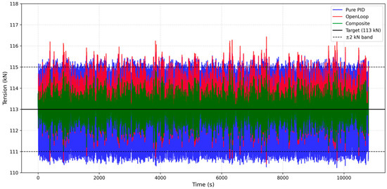
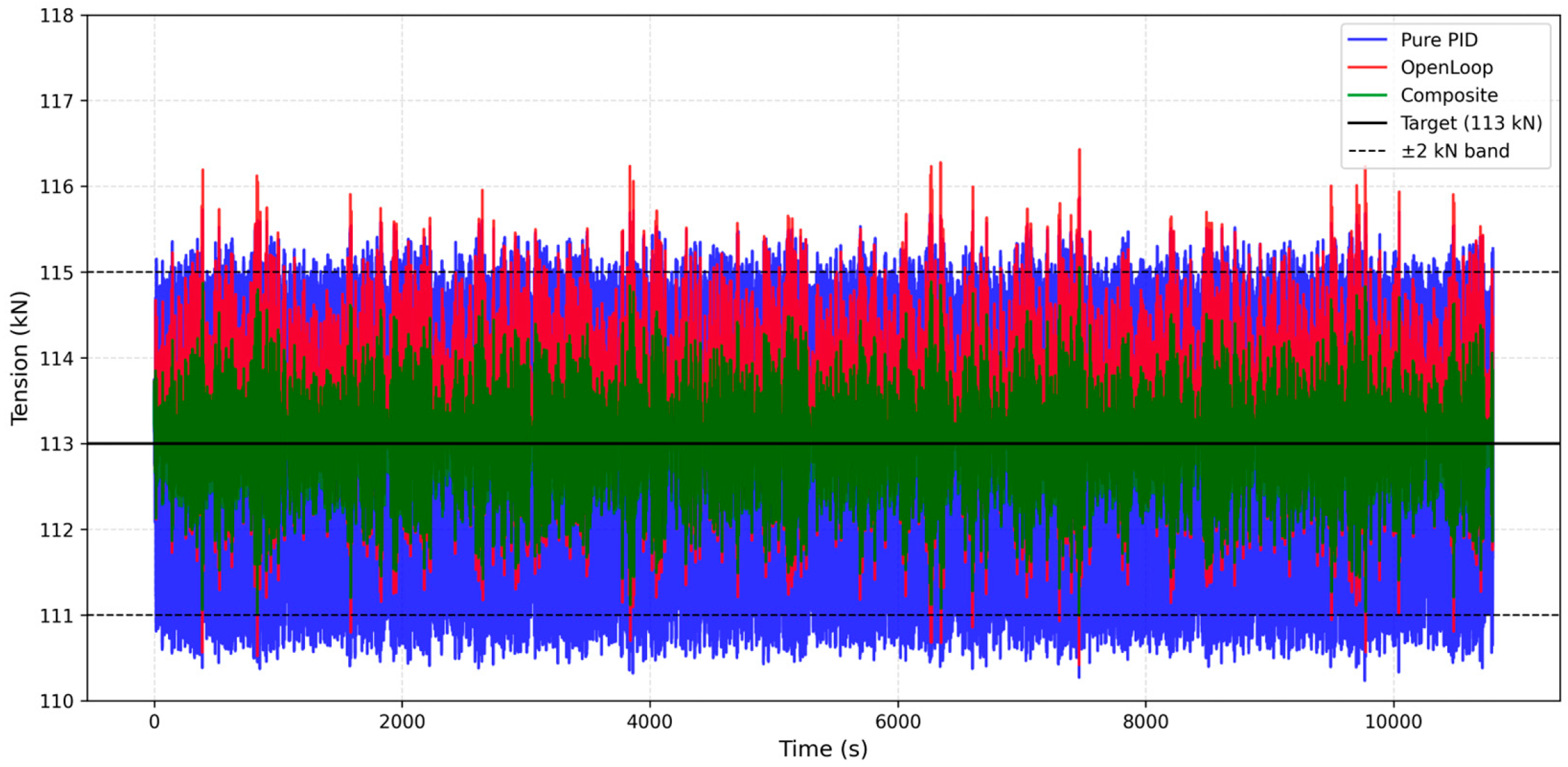
As shown in Figure 16, the open-loop response exhibits significant tension fluctuations, with a peak tension of 116.43 kN. When the pure PID controller is applied, the peak tension is reduced to 115.20 kN. However, the PID response exhibits noticeable oscillations [69].

Figure 16. Performance comparison of three control strategies.

In contrast, the composite control strategy achieves the most favorable performance. All the data lie within the $\pm 2 \mathrm{k}\mathrm{N}$ band. The feedforward component, derived from the SA-CNN predictions, initiates the length adjustment 5 s in advance, effectively counteracting the incoming disturbance before it manifests as a large deviation. The feedback component then compensates for the residual error via the PID controller. As a result, the tension curve under composite control exhibits the smallest amplitudes and the fastest recovery from disturbances. Under this operating condition, the curvature at each moment is less than $0.20 {\mathrm{m}}^{-1}$, which meets the curvature target. Therefore, the curvature constraints do not affect the controller’s decision-making.

As shown in Table 12, the pure PID controller achieves a modest 0.5% reduction in peak tension compared to the open-loop case. However, its RMSE increases significantly from 0.93 to 1.53, representing a 64.52% deterioration relative to the open-loop case. This indicates that although the PID controller reduces the peak value, it introduces severe oscillations into the system, compromising overall stability.

Table 12. Performance comparison of three control strategies.

Strategy	Peak Tension (kN)	${\mathit{R}}_{\mathit{p}\mathit{e}\mathit{a}\mathit{k},\mathit{T}}$ (%)	${\mathit{R}\mathit{M}\mathit{S}\mathit{E}}_{\mathit{T}}$ (kN)
Open loop	116.43	0	0.93
Pure PID	115.87	0.5	1.53
Composite	115.06	1.2	0.55

In contrast, the proposed composite control strategy achieves a 1.2% peak tension reduction—2.4 times that of pure PID—while simultaneously reducing the RMSE to 0.55. This represents a 40.9% improvement over the open-loop case and a 64.0% improvement over pure PID. The composite control strategy not only delivers superior peak reduction but also ensures the most stable performance among all three strategies. The only difference between the pure PID and composite strategies lies in the feedforward component derived from the SA-CNN predictions. The fact that pure PID leads to oscillation while composite control converges smoothly demonstrates that the feedforward prediction effectively suppresses feedback-induced oscillations. It should be noted that due to the inherent physical characteristics of the floating hose, where a 10 m length change produces only approximately 0.1 kN of tension variation, as shown in Section 5.1, the achievable peak reduction via length adjustments is fundamentally limited [44]. The key contribution is not the magnitude of peak reduction itself but the fact that feedforward prediction stabilizes the system where pure PID oscillates, demonstrating the effectiveness of the proposed predictive-control framework.

To verify the functionality of the curvature safety constraint, an additional simulation is performed under the once-in-a-thousand-years sea condition with the hose length of 145 m, where the open-loop curvature exceeds the safety threshold of 0.20 m⁻¹ in some parts.

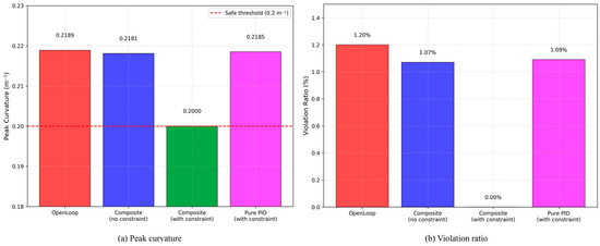
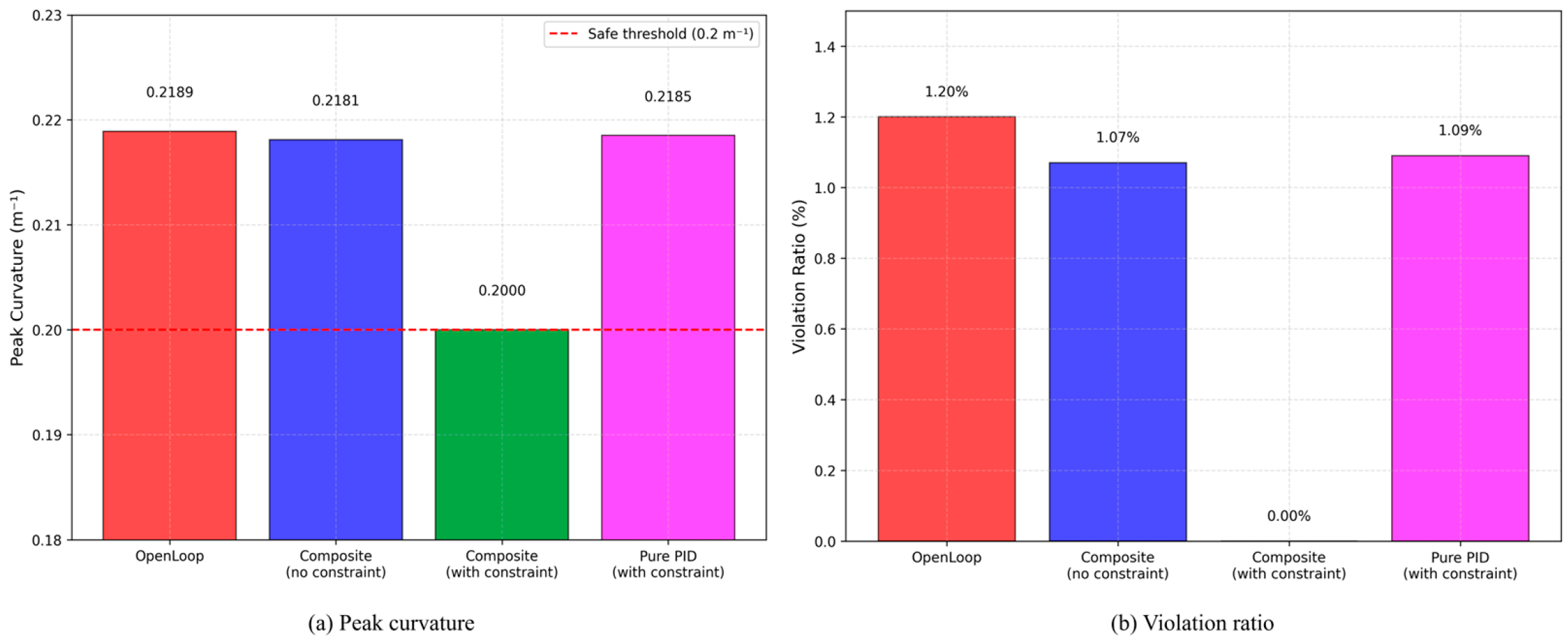
As shown in Figure 17, the peak curvature of the open-loop case is 0.2189 m⁻¹, and the violation ratio is 1.20%. The unconstrained composite control strategy slightly reduces the peak curvature to 0.2181 m⁻¹, with a violation ratio of 1.07%, indicating that its effect on curvature suppression is limited. In contrast, when the curvature safety constraint is activated, the composite control strategy with the curvature constraint successfully limits the peak curvature to 0.2000 m⁻¹ (the preset safety threshold), completely eliminating violations (0.00%). This shows that the proposed constraint mechanism can precisely intervene when the curvature approaches the limit, effectively preventing excessive curvature. The pure PID controller with constraints yields a peak curvature of 0.2185 m⁻¹ and a violation ratio of 1.09%, which is worse than the constrained composite control strategy. These results confirm that the composite control strategy with curvature safety constraints can provide the most reliable protection against excessive curvature in extreme sea conditions, fully verifying the effectiveness of the proposed constraint mechanism.

Figure 17. Curvature constraint performance. (a) Peak curvature; (b) violation ratio.

While the proposed framework demonstrates promising results, several limitations must be acknowledged. First, all results are based on numerical simulations using OrcaFlex. Full-scale field validation has not been conducted, and the actual performance of the system in real offshore environments may differ due to unmodelled effects, such as wave–current misalignments and second-order drift forces. Second, the SA-CNN model is trained on the dataset covering only three sea states (once in a year, once in a century, and once in a thousand years) and three hose lengths (145 m, 150 m, and 155 m). Although the generalization performance of the model has been studied, it cannot be fully guaranteed. Third, the controller parameters are tuned specifically for the hose system considered in this study. For hoses with different parameters, the controller would require retuning to maintain optimal performance.

Future work will address these limitations through: (1) full-scale field trials on a vessel to validate the control performance under realistic sea conditions; (2) physics-informed neural network-based prediction that incorporates the governing equations of hose dynamics to improve extrapolation capabilities; and (3) adaptive controller retuning using reinforcement learning to handle variations in hose properties and environmental conditions.

6. Conclusions

In response to the heightened requirements for safety and stability in the floating hose transfer of solid particles during ship-to-ship and platform-to-ship operations, this study proposes a systematic framework integrating neural network prediction and a feedforward–feedback composite control strategy. The main conclusions are as follows:

(1)

SA-CNN performs the best in the prediction of tension and curvature. Among the four neural network models, SA-CNN achieves the highest R² scores in all nine combinations of hyperparameters and all operating conditions, demonstrating that the spatial attention mechanism effectively enhances feature extraction and improves generalization performance across operating conditions. The prediction step size is a decisive factor affecting accuracy, and the marginal effect of the historical window length decreases.

(2)

The proposed feedforward–feedback composite control strategy significantly outperforms pure PID feedback control. Under the once-in-a-year sea condition, the composite strategy achieves a 1.2% peak tension reduction—2.4 times that of pure PID—while reducing RMSE to 0.55, representing a 40.9% improvement over the open-loop case and a 64.0% improvement over pure PID. More importantly, pure PID introduces severe oscillations, whereas the composite control strategy converges smoothly, demonstrating that feedforward prediction effectively suppresses feedback-induced oscillations.

(3)

The integrated sensing–prediction–decision–execution system is theoretically validated. By sensing real-time 6-DOF ship motions, SA-CNN predicts future tension and curvature, and then the feedforward–feedback controller generates length adjustment commands to drive the active tensioning system. Moreover, the proposed curvature constraint mechanism is shown to be effective under extreme sea conditions, preventing excessive curvature. Although the achievable peak reduction via length adjustments is fundamentally limited by the inherent physical characteristics of the floating hose, where a 10 m length change produces only approximately 0.1 kN of tension variation, the proposed framework ensures system stability and reliability.

This study provides an innovative technical method for the safe operation of floating hoses and granulating flow transportation. Meanwhile, this study offers theoretical support for the intelligent control of flexible hoses. It is expected to play a positive role in high-pressure fracturing fluid transportation for offshore reservoir stimulation and offshore mining solid particle transfer, thus offering promising engineering applicability.

References

- Onwumelu, D.C.; Onwuka, M.K.; Nnebeana, S.E.; Okoro, T.C.; Ekeocha, A.F.; Offurum, C.C.; Ndubuisi, V.N. Crude oil and the problem of wax deposition on pipeline systems during transportation: A review. World J. Adv. Res. Rev. 2022, 15, 781–798. [Google Scholar] [CrossRef] [Scilit]
- Yang, L.; Chen, X.; Luo, L.; Wu, X.; Jing, F. Effect of particle parameters on the hydraulic transport characteristics in a vertical pipeline for deep-sea mining. Ocean Eng. 2025, 321, 120408. [Google Scholar] [CrossRef] [Scilit]
- Li, Y.; Liu, S.; Hu, X. Solid–liquid two-phase flow in deep-sea mining pipelines based on CFD–DEM. Ships Offshore Struct. 2023, 18, 1617–1625. [Google Scholar]
- Zhang, X.; Huang, W.; Ma, W.; Su, L.; Tian, H.; Yang, Y. Cross-sectional mechanical characteristics and sensitivity analysis of unbonded flexible risers under axial loads. J. Ocean Eng. Sci. 2023, 10, 549–560. [Google Scholar] [CrossRef] [Scilit]
- Reddy, N.; Pothal, J.; Barik, R.; Senapati, P. Pipeline slurry transportation system: An overview. J. Pipeline Syst. Eng. Pract. 2023, 14, 03123001. [Google Scholar] [CrossRef] [Scilit]
- Yoon, C.-H.; Lee, D.-K.; Kwon, K.-S.; Kwon, S.-K.; Kwon, O.-K.; Park, Y.-C.; Sung, W.-M. The Effects of Pipe Curvature on the Flow Characteristics of Solid-liquid Two-phase Mixture in an Experimental Flexible Hose System. Geosystem Eng. 2002, 5, 1–7. [Google Scholar] [CrossRef] [Scilit]
- Campello, G.; de Sousa, J.; Vardaro, E. An analytical approach to predict the fatigue life of flexible pipes inside end fittings. In Proceedings of the Offshore Technology Conference, Houston, TX, USA, 2–5 May 2016. [Google Scholar]
- de Sousa, J.R.M.; de Sousa, F.J.; de Siqueira, M.Q.; Sagrilo, L.V.; de Lemos, C.A.D. A theoretical approach to predict the fatigue life of flexible pipes. J. Appl. Math. 2012, 2012, 983819. [Google Scholar] [CrossRef] [Scilit]
- Kang, H.-S.; Kim, M.-H.; Aramanadka, S.B.; Kang, H.-Y.; Lee, K.-Q. Suppression of tension variations in hydro-pneumatic riser tensioner by using force compensation control. Ocean Syst. Eng. 2017, 7, 225–246. [Google Scholar] [CrossRef] [Scilit]
- Jian, W.; Cao, D.; Lo, E.Y.; Huang, Z.; Chen, X.; Cheng, Z.; Gu, H.; Li, B. Wave runup on a surging vertical cylinder in regular waves. Appl. Ocean Res. 2017, 63, 229–241. [Google Scholar] [CrossRef] [Scilit]
- Wang, X.; Qiao, D.; Jin, L.; Yan, J.; Wang, B.; Li, B.; Ou, J. Numerical investigation of wave run-up and load on heaving cylinder subjected to regular waves. Ocean Eng. 2023, 268, 113415. [Google Scholar] [CrossRef] [Scilit]
- Zhang, Y.; Han, Z.; Zhou, X.; Li, B.; Zhang, L.; Zhen, E.; Wang, S.; Zhao, Z.; Guo, Z. METO-S2S: A S2S based vessel trajectory prediction method with Multiple-semantic Encoder and Type-Oriented Decoder. Ocean Eng. 2023, 277, 114248. [Google Scholar] [CrossRef] [Scilit]
- Monsalve-Giraldo, J.; Cortina, J.P.; de Sousa, F.J.; Videiro, P.M.; Sagrilo, L.V. Hybrid Parabolic Interpolation–Artificial Neural Network Method (HPI-ANNM) for long-term extreme response estimation of steel risers. Appl. Ocean Res. 2018, 76, 221–234. [Google Scholar] [CrossRef] [Scilit]
- Zhao, Y.; Dong, S.; Jiang, F. Reliability analysis of mooring lines for floating structures using ANN-BN inference. Proc. Inst. Mech. Eng. Part M J. Eng. Marit. Environ. 2021, 235, 236–254. [Google Scholar]
- Mao, Y.; Wang, T.; Duan, M. A DNN-based approach to predict dynamic mooring tensions for semi-submersible platform under a mooring line failure condition. Ocean Eng. 2022, 266, 112767. [Google Scholar] [CrossRef] [Scilit]
- Yan, J.; Zhang, Y.; Su, Q.; Li, R.; Li, H.; Lu, Z.; Lu, H.; Lu, Q. Time series prediction based on LSTM neural network for top tension response of umbilical cables. Mar. Struct. 2023, 91, 103448. [Google Scholar] [CrossRef] [Scilit]
- Ye, M.; Cao, K.; Wang, J.; Wan, D. Mooring tension prediction of floating offshore wind turbines using end-to-end convolutional neural network models with attention mechanisms. Ocean Eng. 2026, 346, 123939. [Google Scholar] [CrossRef] [Scilit]
- Henry, J.; Collier, L.; Boothe, M.; Campbell, R. Constant Tension Coiler with Electromagnetic Brakes. Patent Application 18/411,389[P], 18 July 2024. [Google Scholar]
- Li, Y.; Wu, S.; Liu, C.; Lu, Q.; Chen, J.; Yan, J.; Yue, Q. Modelling and control of tension in a flexible pipe tensile armour manufacturing process. Int. J. Adv. Manuf. Technol. 2024, 133, 3927–3936. [Google Scholar] [CrossRef] [Scilit]
- Wang, B.; He, D.; Xie, X.; Dai, H.; Li, C. Design and Simulation of Anti Recoil Valve of Riser Tensioner. Chin. Hydraul. Pneum. 2021, 45, 108–121. [Google Scholar]
- Wang, J.; Liu, X.; Chai, J.; Wang, Y.; Jin, X.; He, Z.; Cai, W.; Guo, R. Numerical and experimental investigation on active hydraulic tensioner system for a TLP under tether fails condition. Mar. Struct. 2025, 99, 103693. [Google Scholar] [CrossRef] [Scilit]
- Zhu, H.; Zhang, L.; Yang, J.; Zhang, J.; Gao, B.; Yan, X. A new prediction method for mooring tension of semi-submersible platforms based on SMVMD and deep learning. Ocean Eng. 2026, 357, 125508. [Google Scholar] [CrossRef] [Scilit]
- Ma, G.; Jiang, H.; Chen, H.; Sun, K.; Zhang, J.; Yang, H. Prediction of FOWT mooring tension during non-stationary typhoon transit: A Transformer based framework with Bayesian optimization. Ocean Eng. 2026, 353, 124758. [Google Scholar] [CrossRef] [Scilit]
- Lyu, F.; Ji, C.; Xu, S.; Lu, L.; Hao, Y. Short-term prediction of mooring tension for floating breakwater based on the LSTM-ASSA-Transformer method. Ocean Eng. 2025, 342, 123087. [Google Scholar] [CrossRef] [Scilit]
- Zhao, Y.; Dong, S.; Jiang, F.; Incecik, A. Mooring tension prediction based on BP neural network for semi-submersible platform. Ocean Eng. 2021, 223, 108714. [Google Scholar] [CrossRef] [Scilit]
- Li, J.; Zhan, K.; Zhang, M.; Cheng, Y.; Wang, Y. The Spatial Configuration and Force Analyses of Hoses in a Fully Hose-Based Conveyance System. J. Mar. Sci. Eng. 2025, 13, 1395. [Google Scholar] [CrossRef] [Scilit]
- Abu-Sena, A.B.B.; Soliman, M.S.A.-D.; Abdel-Nabi, O.N.A. Behavior and resistance of beam-column structural elements. J. Constr. Steel Res. 2012, 71, 171–181. [Google Scholar] [CrossRef] [Scilit]
- Feng, Y.; Zhang, B.; Chen, Y.; Wang, B.; Xia, H.; Yu, H.; Yu, X.; Yang, P. Research on Cantilever Beam Roller Tension Sensor Based on Surface Acoustic Wave. Micromachines 2025, 16, 1044. [Google Scholar] [CrossRef] [Scilit] [PubMed]
- Bauchau, O.A.; Craig, J.I. Euler-Bernoulli beam theory. In Structural Analysis; Springer: Berlin/Heidelberg, Germany, 2009; pp. 173–221. [Google Scholar]
- Dong, S.; Dong, B.; Yu, C.; Guo, Y. High sensitivity optical fiber curvature sensor based on cascaded fiber interferometer. J. Light. Technol. 2018, 36, 1125–1130. [Google Scholar] [CrossRef] [Scilit]
- Such, M.; Jimenez-Octavio, J.R.; Carnicero, A.; Lopez-Garcia, O. An approach based on the catenary equation to deal with static analysis of three dimensional cable structures. Eng. Struct. 2009, 31, 2162–2170. [Google Scholar] [CrossRef] [Scilit]
- Zhang, C.; Wu, F.; Huang, M.; Ma, J.; Ma, H.; Liu, Y. Generative AI for Planar Substrate Integrated Waveguide Microwave Filters: Autonomous Circuit Synthesis With Coupling-Controlled Topology Generation. IEEE Trans. Microw. Theory Tech. 2025, 74, 1740–1755. [Google Scholar]
- Wang, L.; Kang, X.; Ding, F.; Nakagawa, S.; Ren, F. A joint local spatial and global temporal CNN-Transformer for dynamic facial expression recognition. Appl. Soft Comput. 2024, 161, 111680. [Google Scholar] [CrossRef] [Scilit]
- Guzmán, J.L.; Hägglund, T. Tuning rules for feedforward control from measurable disturbances combined with PID control: A review. Int. J. Control 2024, 97, 2–15. [Google Scholar] [CrossRef] [Scilit]
- Knospe, C. PID control. IEEE Control Syst. Mag. 2006, 26, 30–31. [Google Scholar] [CrossRef] [Scilit]
- Lu, K.; Zhou, W.; Zeng, G.; Du, W. Design of PID controller based on a self-adaptive state-space predictive functional control using extremal optimization method. J. Frankl. Inst. 2018, 355, 2197–2220. [Google Scholar] [CrossRef] [Scilit]
- Zhang, S.; Xie, L. A PID controller approach for adaptive probability-dependent gradient decay in model calibration. Adv. Neural Inf. Process. Syst. 2024, 37, 114744–114764. [Google Scholar] [CrossRef] [Scilit]
- Xu, Z.; Liu, X.; Shen, Z. A Kind of Wave Passive Compensation Device’s Rope Tension Research. In Proceedings of the 2016 6th International Conference on Mechatronics, Computer and Education Informationization (MCEI 2016), Shenyang, China, 11–13 November 2016; Atlantis Press: Dordrecht, The Netherlands, 2016; pp. 901–906. [Google Scholar]
- Chen, B.; Yu, J.; Yu, Y.; Xu, L.; Hao, S.; Wu, C.; Wu, H. Study on key performance parameters of hydro-pneumatic tensioner for top tensioned riser. Appl. Ocean Res. 2019, 84, 206–215. [Google Scholar] [CrossRef] [Scilit]
- Li, J.; Kong, L.; Liang, H.; Li, W. Review of development and characteristics research on electro-hydraulic servo system. Recent Pat. Eng. 2024, 18, 140–154. [Google Scholar] [CrossRef] [Scilit]
- Gan, C.; Zhang, S.; Zheng, X.; Zhang, J.; Lu, X. Design and wear protection research of metal hose based on aramid wear-resistant layer. J. Mech. Sci. Technol. 2025, 39, 7463–7472. [Google Scholar] [CrossRef] [Scilit]
- Kang, H.-S.; Kim, M.-H.; Aramanadka, S.S.B. Tension variations of hydro-pneumatic riser tensioner and implications for dry-tree interface in semisubmersible. Ocean Syst. Eng. 2017, 7, 21–38. [Google Scholar] [CrossRef] [Scilit]
- Chinpon, A.; Thamaphat, K.; Hansuparnusorn, M.; Limsuwan, P. A force measurement method using the optical fibre beam. Procedia Eng. 2012, 32, 989–993. [Google Scholar] [CrossRef] [Scilit]
- Hanyu, M.; Zhiyuan, C.; Jingjing, L.; Qidong, F.; Lecheng, L.; Long, Y. Modelling and analysis of long floating hose string at different working states during the pumping ashore process. Ships Offshore Struct. 2025, 20, 1118–1130. [Google Scholar] [CrossRef] [Scilit]
- Xu, Z.; Shen, T.; Zhang, X.; Chen, M. The conceptual design of a novel offshore borehole mining technology and study on granularization principle. J. Ocean Eng. Sci. 2026, 11, 638–648. [Google Scholar] [CrossRef] [Scilit]
- Mahmoud, R.M.A.; Dodds, P.E. A technical evaluation to analyse of potential repurposing of submarine pipelines for hydrogen and CCS using survival analysis. Ocean Eng. 2022, 266, 112893. [Google Scholar] [CrossRef] [Scilit]
- Lu, Z.; Liu, X.; Pan, B. Numerical simulation of cylindrical particles conveying in curved ducts using CFD-DEM coupled approach. China Powder Sci. Technol. 2011, 17, 65–69. [Google Scholar]
- Zhang, F.; Zhang, Y.; Li, Z.; An, C.; Li, L. Theoretical and FEA investigation of the mechanical behaviour for offshore LCO2 floating hose. Ocean Eng. 2024, 312, 119107. [Google Scholar] [CrossRef] [Scilit]
- Rueda-Bayona, J.G.; Guzmán, A.; Cabello Eras, J.J. Selection of JONSWAP spectra parameters during water-depth and sea-state transitions. J. Waterw. Port Coast. Ocean Eng. 2020, 146, 04020038. [Google Scholar] [CrossRef] [Scilit]
- Wiles, T. Reliability of numerical modelling predictions. Int. J. Rock Mech. Min. Sci. 2006, 43, 454–472. [Google Scholar] [CrossRef] [Scilit]
- Gonzalez, G.M.; de Sousa, J.R.; Sagrilo, L.V. A study on the axial behavior of bonded flexible marine hoses. Mar. Syst. Ocean Technol. 2016, 11, 31–43. [Google Scholar] [CrossRef] [Scilit]
- Herdzik, J. Possibilities of improving safety and reliability of ship propulsion system during dp operations. J. KONES. Powertrain Transp. 2015, 19, 219–226. [Google Scholar]
- Ja’e, I.A.; Ali, M.O.A.; Yenduri, A.; Amaechi, C.V.; Nizamani, Z.; Nakayama, A. Optimization of mooring line design parameters using Mooring Optimization Tool for FPSO (MooOpT4FPSO) with the consideration of integrated design methodology. Ocean Eng. 2022, 264, 112499. [Google Scholar] [CrossRef] [Scilit]
- Schober, P.; Boer, C.; Schwarte, L.A. Correlation coefficients: Appropriate use and interpretation. Anesth. Analg. 2018, 126, 1763–1768. [Google Scholar] [CrossRef] [Scilit] [PubMed]
- Obilor, E.I.; Amadi, E.C. Test for significance of Pearson’s correlation coefficient. Int. J. Innov. Math. Stat. Energy Polic. 2018, 6, 11–23. [Google Scholar] [CrossRef]
- Zhang, X.; Wang, J.; Ma, J.; Wang, D.; Lu, G.; Wei, J.; Wang, Y.; Wang, G. Data-driven approaches to predicting six-degree-of-freedom ship motion under irregular sea states. Chem. Prod. Process Model. 2025. [Google Scholar] [CrossRef] [Scilit]
- Taylor, G.W.; Fergus, R.; LeCun, Y.; Bregler, C. Convolutional learning of spatio-temporal features. In Proceedings of European Conference on Computer Vision; Springer: Berlin/Heidelberg, Germany, 2010; pp. 140–153. [Google Scholar]
- Watson, D.S.; Wright, M.N. Testing conditional independence in supervised learning algorithms. Mach. Learn. 2021, 110, 2107–2129. [Google Scholar] [CrossRef] [Scilit]
- Crowther, P.S.; Cox, R.J. A method for optimal division of data sets for use in neural networks. In Proceedings of International Conference on Knowledge-Based and Intelligent Information and Engineering Systems; Springer: Berlin/Heidelberg, Germany, 2005; pp. 1–7. [Google Scholar]
- Mlodozeniec, B.; Reisser, M.; Louizos, C. Hyperparameter optimization through neural network partitioning. arXiv 2023, arXiv:2304.14766. [Google Scholar]
- Miranda, C.S.; Von Zuben, F.J. Reducing the training time of neural networks by partitioning. arXiv 2015, arXiv:1511.02954. [Google Scholar]
- Yao, Y.; Rosasco, L.; Caponnetto, A. On early stopping in gradient descent learning. Constr. Approx. 2007, 26, 289–315. [Google Scholar] [CrossRef] [Scilit]
- Zhang, T.; Sun, J.; Zhang, Q.; Cheng, J.; Yuan, P. Multi-step prediction of wind power ramping based on dynamic historical window adjustment. Energy Rep. 2025, 14, 1708–1716. [Google Scholar] [CrossRef] [Scilit]
- Wang, L.; Liu, N.; Wang, S.; Chen, S. Study on cable tension characteristics of shore-based constant tension mooring systems under the coupling effect of wind, wave, and current. J. Offshore Mech. Arct. Eng. 2024, 146, 051704. [Google Scholar] [CrossRef] [Scilit]
- Lee, C.F.; Ong, M.C. Numerical analysis of mooring systems for reducing peak mooring line tensions in a combined wind and wave energy system at an intermediate water depth. Ocean Eng. 2025, 325, 120767. [Google Scholar] [CrossRef] [Scilit]
- Hambali, N.; Masngut, A.; Ishak, A.A.; Janin, Z. Process controllability for flow control system using Ziegler-Nichols (ZN), Cohen-Coon (CC) and Chien-Hrones-Reswick (CHR) tuning methods. In Proceedings of 2014 IEEE International Conference on Smart Instrumentation, Measurement and Applications (ICSIMA); IEEE: Piscataway, NJ, USA, 2014; pp. 1–6. [Google Scholar]
- Muresan, C.I.; De Keyser, R. Revisiting Ziegler–Nichols. A fractional order approach. ISA Trans. 2022, 129, 287–296. [Google Scholar] [CrossRef] [Scilit] [PubMed]
- Joseph, S.B.; Dada, E.G.; Abidemi, A.; Oyewola, D.O.; Khammas, B.M. Metaheuristic algorithms for PID controller parameters tuning: Review, approaches and open problems. Heliyon 2022, 8, e09399. [Google Scholar] [CrossRef] [Scilit] [PubMed]
- Yüksek, G. A novel delay-affected two degree of freedom PID controller using physics-inspired optimization for robust control applications. Sci. Rep. 2025, 16, 3453. [Google Scholar] [CrossRef] [Scilit] [PubMed]
Disclaimer/Publisher’s Note: The statements, opinions and data contained in all publications are solely those of the individual author(s) and contributor(s) and not of MDPI and/or the editor(s). MDPI and/or the editor(s) disclaim responsibility for any injury to people or property resulting from any ideas, methods, instructions or products referred to in the content. |
© 2026 by the authors. Licensee MDPI, Basel, Switzerland. This article is an open access article distributed under the terms and conditions of the Creative Commons Attribution (CC BY) license.