Methodologies for Underwater Geomagnetic Navigation: Progress and Prospects

Abstract

High-precision, long-endurance navigation remains a central bottleneck for autonomous underwater vehicles (AUVs) operating in GNSS-denied, acoustically constrained, and dynamically disturbed marine environments. This manuscript examines the complete sensing-mapping-estimation chain for underwater geomagnetic navigation. It distinguishes scalar and vector measurements; compares shipborne, towed, and AUV-mounted survey configurations, calibration requirements, platform-interference mitigation, and uncertainty sources; reviews global, regional, and local magnetic models; and evaluates nonlinear map-aided positioning. Existing approaches are organized into map-based matching, filter-aided navigation, geomagnetic simultaneous localization and mapping (SLAM), and matching-area adaptability assessment. Their assumptions, data requirements, uncertainty treatment, accuracy evidence, and computational burden are critically compared. Persistent gaps include magnetic cleanliness, three-dimensional mapping, weak-feature-area observability, benchmark datasets, uncertainty quantification, and reproducible long-duration sea trials.

1. Introduction

The growing demand for persistent underwater observation, seabed resource exploration, subsea infrastructure inspection, and marine environmental monitoring has placed stricter requirements on autonomous underwater vehicles’ (AUVs) autonomy. In these missions, navigation errors do not merely degrade position estimates; they directly affect path planning, sampling quality, revisit accuracy, and mission safety [1]. Therefore, underwater navigation should be evaluated not only by nominal positioning accuracy but also by endurance, infrastructure dependence, observability, environmental robustness, and operational covertness [2].

Conventional underwater navigation combines acoustic positioning, inertial navigation, Doppler velocity logs (DVLs), and occasional surface or external fixes. Acoustic systems can provide bounded local accuracy but depend on infrastructure and are vulnerable to multipath, attenuation, and geometry [3]. An inertial measurement unit (IMU) contains accelerometers and gyroscopes, whereas an inertial navigation system (INS) combines IMU measurements with mechanization and estimation algorithms to compute position, velocity, and attitude. INS errors grow with time because sensor biases are integrated [4]. These limitations motivate passive, infrastructure-independent geophysical aiding methods for long-duration missions.

As a geophysical-field-aided navigation approach, geomagnetic navigation is attractive because the Earth’s magnetic field is globally available, does not require active signal emission, and contains spatial anomaly information that can be used as a natural fingerprint [5]. Nevertheless, these advantages are conditional [6]. The usable navigation information depends on anomaly distinctiveness, map resolution, temporal correction, sensor installation, vehicle magnetic cleanliness, and the matching algorithm’s ability to reject ambiguous or weak-feature areas [7,8].

The foundational concepts of modern geomagnetic navigation emerged in the 1960s from British and American researchers, leading to the US development of the Magnetic Contour Matching (MATCOM) system [9,10,11]. In the mid-1970s, the former Soviet Union’s Ramenskoye company conducted the pioneering MAGNET experiment, which used geomagnetic field strength as a characteristic quantity for contour-based guidance, marking a crucial demonstration of practical feasibility [12].

During the 1980s, the US systematically elaborated methods for autonomous underwater vehicle navigation using geomagnetic fields, while Sweden’s Carl Tyrén initiated related research on ship speed and positioning [13]. By 1997, the US, France and other countries had incorporated geophysical and non-traditional navigation topics into the NTM program, reflecting growing international interest [14,15,16]. Around the turn of the century, the US achieved a breakthrough with a matching system offering accuracies better than 30 m on the ground and in the air, and better than 500 m underwater [17]; concurrently, Russia developed a geomagnetic contour-guided missile system that significantly enhanced operational effectiveness [18].

In 2005, French researchers validated the rich characteristic information of the geomagnetic field, confirming its ability to meet stringent missile guidance requirements [19]. In 2006, Goodrich Corporation introduced a novel speed-and-positioning method based on three-dimensional geomagnetic maps, demonstrating that vector matching between the field’s three components and the map could achieve accurate navigation and positioning [20]. In 2009, Japan advanced the field by simulating matching algorithms using measured geomagnetic and bathymetry data, verifying their validity for practical underwater and aerial navigation systems [21]. These collective developments trace the evolution of geomagnetic navigation from its conceptual origins to a viable, precise solution with expanding applications.

China’s geomagnetic navigation research began later than that of leading nations but accelerated steadily after the 11th Five-Year Plan (2006–2010) when the government recognized its strategic value. Early systematic efforts included CASIC’s 2004 static experiments, which first validated the feasibility of geomagnetic matching [22,23]; NUDT’s development and multi-environment testing of a GAINS prototype (2007–2011) [23]; NWPU’s 2007 demonstration that geomagnetic data could correct INS errors [24]; Wuhan University’s 2008 underwater trial in Bohai Bay, achieving 100 m localization accuracy [25]; Peking University’s 2010 research attaining ~400 m accuracy and stressing the need for high-resolution maps [26]; and Qiao Hong et al.’s 2012 multi-sensor fusion framework integrating magnetic, gravity and other data to improve robustness [27].

Subsequent algorithmic innovations further advanced underwater navigation. In 2013, Wang Shengping et al. proposed an improved TERCOM algorithm using Hausdorff distance, reaching ≤100 m positioning and 0.4° heading correction in Bohai Sea trials [28]. Liu Mingyong et al. (2015) designed a particle-filter-based dynamic correction to mitigate geomagnetic interference [29]; Li Hong et al. (2017) introduced an evolutionary search method with ocean current compensation to counter AUV trajectory drift [30]; Chong Yang et al. (2021) developed a fuzzy-decision adaptability evaluation model to select high-information areas and reduce INS cumulative errors [31]; Chong Yang et al. (2022) combined PCA and an improved BP neural network for self-organizing classification of candidate matching regions [32]; and Huapeng Yu et al. (2023) proposed adaptive split particle filtering to address particle degradation and impoverishment, further improving matching accuracy [33].

Current research on underwater geomagnetic navigation revolves around three coupled problems, credible measurement, reliable reference-map construction, and robust positioning-model design, whose independent treatment can obscure error propagation. In data measurement and processing, efforts focus on high-precision sensors and advanced signal processing (e.g., adaptive filtering and machine learning) to suppress noise and interference in dynamic underwater environments [34]. For reference-map construction, multi-source data (satellites, marine surveys, AUVs) are integrated using geospatial interpolation and machine-learning generation, while real-time updating mechanisms are being explored to handle temporal field variations caused by solar activity and geological changes [35,36].

The development of matching and filtering algorithms is a cornerstone of the field. Kalman and particle filtering techniques are widely used to fuse geomagnetic data with inertial navigation systems (INS), reducing cumulative errors and improving long-term accuracy [37,38]. Geomagnetic matching itself aligns real-time measurements with pre-constructed maps by identifying distinctive features (anomalies, gradients); recent innovations in pattern recognition and optimization, genetic algorithms and deep-learning approaches, have enhanced efficiency and accuracy, even in regions with weak or complex signatures [39]. Beyond these, integrating Simultaneous Localization and Mapping (SLAM) with geomagnetic navigation has emerged as a promising solution for long-term autonomous navigation, enabling real-time environment mapping alongside positioning, particularly valuable for underwater robotics and subsea inspection where prior maps are limited [40].

The primary objective of this review is not merely to summaries existing methods but to clarify technical bottlenecks that hinder transition from experimental demonstrations to reliable AUV deployment. Specifically, the review addresses four questions: (i) which geomagnetic feature quantities are observable and stable underwater; (ii) how measurement errors, vehicle interference, and environmental disturbances propagate into positioning; (iii) which categories of matching, filtering, and SLAM algorithms suit different map-availability and computational constraints; and (iv) what evidence is still missing for large-scale, long-duration, and reproducible validation [41].

By systematically analyzing current technologies, the paper identifies key challenges and gaps. For example, matching achieves high localized accuracy but performs poorly in weak-feature or high-noise regions, necessitating further signal-processing and feature-extraction advances [42]; geomagnetic SLAM, though promising, faces computational efficiency and scalability issues in large-scale environments [43]. Future directions include adaptive machine-learning data processing, multi-sensor fusion frameworks, and real-time map updating to account for temporal variations [44]. To strengthen review logic, subsequent sections follow a problem-driven taxonomy, measurement credibility, map reliability, algorithm applicability, and operational adaptability, separating mature practices from open problems, thereby supporting method selection, experimental design, and future development of reliable AUV navigation systems.

Review Scope and Methodology

This is a structured narrative review, not a systematic review or meta-analysis. The literature is organized around five themes: magnetic measurement and calibration; reference-field and local-map construction; map-aided matching and nonlinear filtering; and geomagnetic SLAM or adaptability assessment. Search terms included combinations of underwater geomagnetic navigation, magnetic anomaly navigation, map-aided navigation, magnetic matching, geomagnetic filtering, magnetic SLAM, and AUV magnetometer. Studies were retained if they contributed a measurement method, model, algorithm, experiment, or critical assessment directly relevant to autonomous navigation; works on magnetic target detection or unrelated indoor positioning were used only when their methods were transferable and this limitation was stated. The literature is classified by theme, publication period, sensing configuration, map dependence, estimation model, and geographical contribution. Because reporting standards and public datasets remain heterogeneous, the review emphasizes assumptions and evidence quality rather than ranking methods solely by reported accuracy.

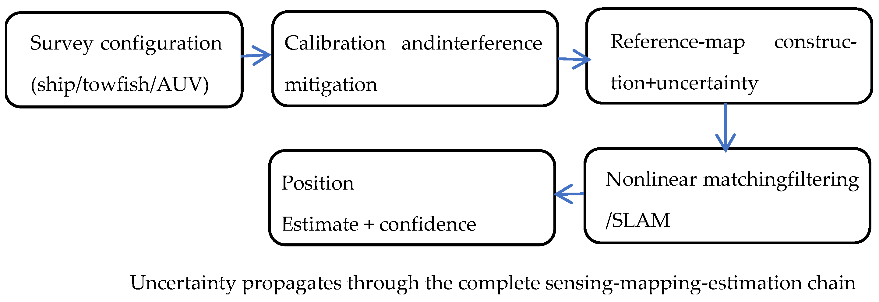
The review’s original contribution is a problem-driven synthesis that connects measurement uncertainty to map reliability and estimator performance. As shown in Figure 1. This organization distinguishes mature engineering practice from open research problems and identifies the minimum information that future experiments should report to ensure reproducibility.

2. Key Technologies for Underwater Geomagnetic Navigation

This section reorganises the enabling technologies of underwater geomagnetic navigation according to the problem chain that determines positioning performance. Instead of treating sensing, mapping, and algorithms as independent modules, the review emphasises their coupling. Feature selection determines what can be measured; measurement quality determines the fidelity of the reference map; map resolution and uncertainty determine the discriminability of candidate matching areas; and the positioning algorithm determines how sensor, map, and motion uncertainties are propagated and constrained.

The first critical issue is feature observability, which concerns selecting geomagnetic quantities that are stable, measurable, and spatially discriminative. Equally important is measurement credibility, since accurate acquisition and processing of geomagnetic data are essential for navigation success. High-precision sensors such as fluxgate magnetometers and proton precession magnetometers are commonly used, but raw data often contain noise and distortions from sensor drift, ocean currents, and external magnetic interference. To address these challenges, advanced signal processing techniques, including wavelet transforms, Kalman filtering, and adaptive filtering, have been employed to denoise and enhance data quality [6]. Furthermore, machine learning-based approaches, such as deep neural networks, have shown promise in improving accuracy and efficiency, particularly in dynamic and noisy underwater environments [45].

Map reliability is another cornerstone of map-dependent navigation. The construction of high-resolution local geomagnetic reference maps must be discussed in terms of resolution, interpolation uncertainty, altitude or depth dependence, temporal correction, and survey repeatability. Without explicit map uncertainty, a matching algorithm may return an apparently precise but physically ambiguous position in low-information or poorly surveyed areas.

Regarding algorithm applicability, the design of effective geomagnetic positioning methods should be driven by the available information rather than by algorithm popularity. Correlation matching is transparent but sensitive to ambiguity [46]; ICP and ICCP type methods exploit geometric similarity but depend on good initialisation [47]; filtering methods provide recursive uncertainty propagation but require reliable process and observation models; and SLAM reduces dependence on prior maps but increases requirements for loop closure, map representation, and computation.

In summary, the key technologies in underwater geomagnetic navigation are interconnected and collectively contribute to the development of highly accurate and reliable systems. By addressing the challenges associated with feature selection, data measurement and processing, map construction, and positioning method design, researchers and engineers can continue to advance the field and expand the applicability of geomagnetic navigation in diverse underwater applications.

2.1. Underwater Geomagnetic Feature Selection

The selection of appropriate feature quantities is the first observability problem in underwater geomagnetic navigation. A useful feature should be stable over the mission period, measurable with the available magnetometer configuration, sufficiently variable within the operating area, and insensitive to vehicle attitude errors. Therefore, the choice of total-field intensity, vector components, gradients, or anomaly derived descriptors should be justified by the operating scenario rather than assumed a priori.

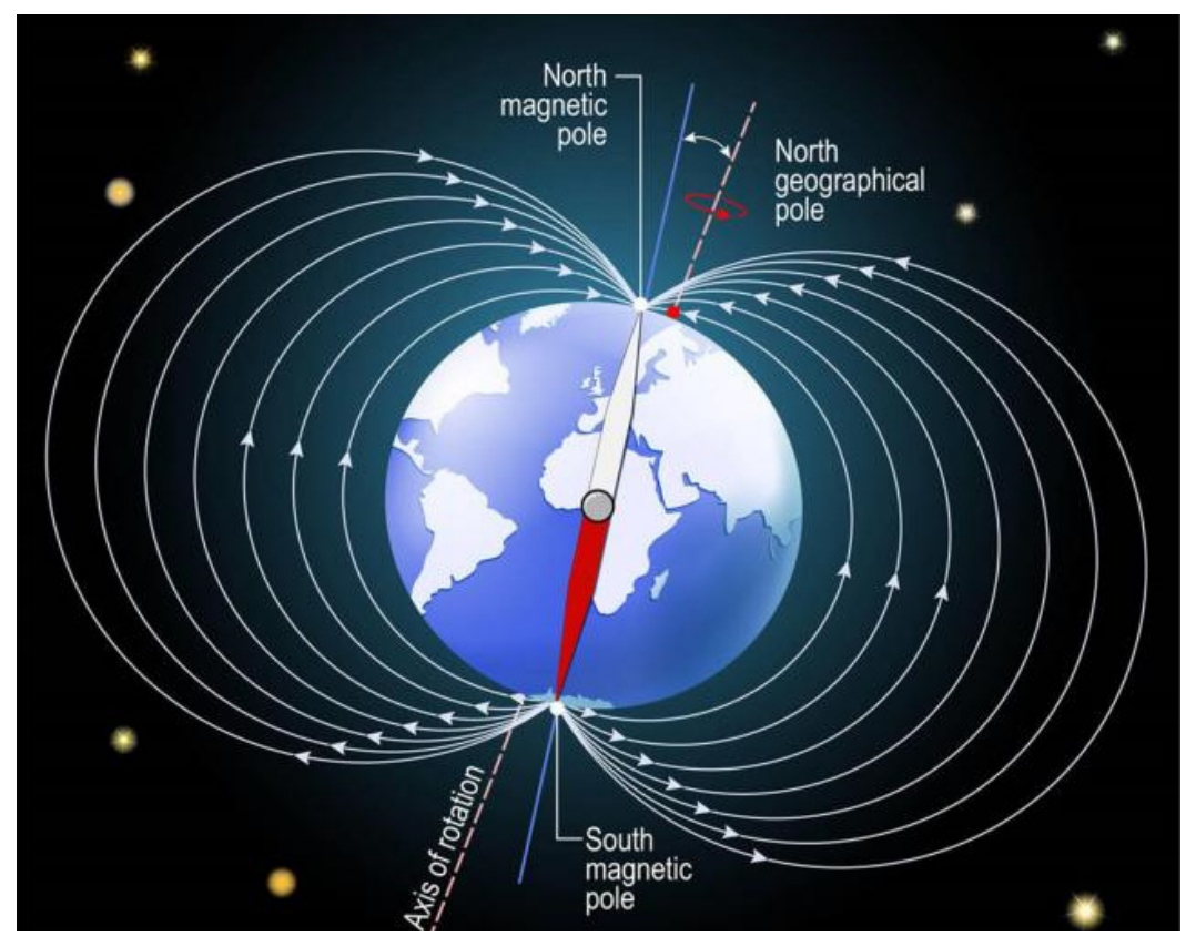
The geomagnetic field can be modeled as the magnetic field generated by a magnetic dipole situated at the Earth’s center, and its distribution exhibits a relatively stable pattern across the planet’s surface, and the distribution of the geomagnetic field is shown in Figure 2.

Based on empirical geomagnetic measurements, it has been determined that the average magnetic field strength at the Earth’s surface is approximately 5 × 10⁴ nanotesla (nT), with the highest intensities observed at the magnetic poles, where the geomagnetic field strength reaches approximately 7 × 10⁴ nT. This relatively small variation in geomagnetic field strength underscores the importance of minimizing external perturbations during geomagnetic field measurements to ensure data accuracy. The geomagnetic field is composed of three primary components: the main geomagnetic field, the geomagnetic anomaly field, and the perturbation field. The main geomagnetic field is generated by the dynamic interactions of high-temperature and high-pressure materials within the Earth’s core. The geomagnetic anomaly field, which accounts for only about 4% of the total geomagnetic field, is primarily caused by magnetized crustal rocks and exhibits minimal temporal variation. In contrast, the perturbation field, which is strongly influenced by solar activity, exhibits significant variability, with strengths ranging from approximately 5 nT to 500 nT, and can change rapidly over short time scales [48]. Given the relative stability of the main geomagnetic field and the geomagnetic anomaly field, these components are typically utilized in geomagnetic matching navigation systems.

The geomagnetic field may be written as the magnetic flux-density vector B = [X, Y, Z]^T. In conventional geomagnetic notation, F = |B| is total intensity, H = $\sqrt{({\mathrm{X}}^2+{\mathrm{Y}}^2)}$ is horizontal intensity, D = atan²(Y, X) is declination, and I = atan²(Z, H) is inclination. Thus, F is the scalar magnitude of B, while X, Y, and Z are its components in a specified navigation or geodetic frame. Fluxgate magnetometers measure vector components and therefore require calibration and attitude knowledge; proton-precession and Overhauser instruments measure scalar F and do not directly provide direction. For moving underwater platforms, feature selection must consider observability, attitude sensitivity, temporal stability, and spatial distinctiveness. In many mid-latitude AUV scenarios, F or gradients are more robust than D or I, whose useful variation may be small relative to attitude and installation errors [49,50].

In underwater geomagnetic navigation, the measurement methodology is critical to achieving high accuracy. Underwater carriers typically employ a towed measurement system, where the magnetometer is deployed behind the carrier to minimize interference from the carrier’s own magnetic field. This approach significantly improves measurement accuracy by reducing the influence of magnetic noise generated by the carrier’s equipment and structure. However, the complexity of the underwater environment introduces challenges related to the stability of the magnetometer’s attitude. Variations in the magnetometer’s orientation due to underwater currents or carrier motion can lead to inaccuracies in the measured data [43]. Furthermore, the attitude of the underwater carrier may differ from that of the magnetometer, adding another layer of complexity to the measurement process. Traditional attitude measurement systems on underwater carriers often fail to provide accurate real-time data on the magnetometer’s orientation in the geodetic coordinate system. This discrepancy arises because the magnetometer may not be synchronized with the carrier’s attitude measurement system, or the system may not accurately reflect the magnetometer’s true orientation due to the unique dynamics of the underwater environment [41].

Given these challenges, the total geomagnetic field strength (F) is often preferred as the characteristic quantity for underwater navigation and localization [49,50,51]. This preference stems from the relative stability and ease of measurement of the total geomagnetic field strength, making it well-suited for use in the dynamic and often unpredictable underwater environment. In underwater geomagnetic navigation systems, sensors such as optical pump magnetometers or fluxgate magnetometers are commonly employed. Optical pump magnetometers are capable of directly measuring the total geomagnetic field strength with High precision, while fluxgate magnetometers calculate the total geomagnetic field strength by measuring the three orthogonal components (X, Y, and Z) and combining them through vector summation [52]. The choice of sensor depends on the specific requirements of the navigation system, including measurement accuracy, operational depth, and environmental conditions.

In summary, the selection of geomagnetic matching feature quantities and the design of measurement systems are critical to the success of underwater geomagnetic navigation. By leveraging the stability of the total geomagnetic field strength and employing advanced measurement techniques, researchers and engineers can develop robust navigation systems capable of operating effectively in the challenging underwater environment.

2.2. Underwater Geomagnetic Measurement and Data Processing

Underwater magnetic observations may be acquired using shipborne sensors, a towed towfish, or sensors integrated into an AUV. Shipborne surveys provide endurance and accurate positioning but remain susceptible to vessel fields. Towed systems increase separation from the magnetic platform and are often preferred for scalar mapping, although tow-cable motion, layback estimation, depth variation, and attitude must be modeled. AUV-mounted systems support mission-representative data collection and repeated surveys, but require magnetic-clean design, careful sensor placement, synchronized attitude/depth measurements, and compensation for propulsion, batteries, actuators, and payloads. Calibration should address hard-iron bias, soft-iron scale and non-orthogonality, sensor alignment, temperature dependence, heading error, timing, and position/layback uncertainty. Measurement uncertainty should be propagated into map cells and navigation observations rather than represented by a single nominal sensor accuracy.

A practical measurement campaign should include shore or laboratory calibration, magnetic-cleanliness tests with subsystems switched individually, multi-heading maneuvers when appropriate, repeated reciprocal survey lines, cross-over analysis, diurnal correction using a base station or observatory, and independent validation lines. Accuracy should be reported as a budget containing sensor noise and bias, platform-compensation residuals, attitude and timing errors, navigation/layback errors, depth mismatch, temporal correction, and interpolation uncertainty. The required accuracy is application-dependent: total observation uncertainty must remain sufficiently below the local anomaly contrast and gradient over the intended matching window to preserve location discriminability. The corresponding comparison of magnetometer technologies for underwater geomagnetic navigation is presented in

Table 1. Comparison of Magnetometer Technologies Relevant to Underwater Geomagnetic Navigation.

Magnetometer Technology	Measurement Principle	Typical Sensitivity/Resolution	Advantages for Underwater Navigation	Limitations/Challenges
Fluxgate Magnetometer	Measures magnetic field using saturation of a ferromagnetic core	~10 pT–1 nT	Mature technology; low power; compact; good vector-field measurement; widely used in marine platforms	Requires calibration for bias, scale factor, and soft-/hard-iron effects; temperature drift
Optically Pumped Magnetometer (OPM)	Uses atomic energy-level transitions to measure magnetic field magnitude	~fT–pT	Very high sensitivity; excellent for detecting weak geomagnetic anomalies	Often measures scalar field only; can be larger and more expensive; sensitive to environmental conditions
Proton Precession Magnetometer	Measures precession frequency of hydrogen protons in a magnetic field	~0.1–1 nT	Absolute scalar measurement; stable and reliable; useful for geomagnetic surveys	Lower sampling rate; relatively high power; not ideal for fast maneuvering vehicles
Overhauser Magnetometer	Enhanced proton precession using electron-proton coupling	~0.01–0.1 nT	High accuracy; lower power than proton precession; good scalar stability	Larger than solid-state sensors; scalar-only measurement
SQUID Magnetometer	Uses superconducting quantum interference to measure magnetic flux	~fT or better	Extremely high sensitivity; capable of detecting very weak magnetic signals	Requires cryogenic cooling; expensive; complex; difficult to deploy on small underwater vehicles
AMR Magnetometer	Uses anisotropic magnetoresistance effect	~nT	Small size; low cost; low power; suitable for integrated navigation systems	Lower sensitivity than fluxgate/OPM; temperature and bias drift; needs frequent calibration
GMR Magnetometer	Uses giant magnetoresistance effect	~nT–sub-nT	Compact; low power; higher sensitivity than AMR in some designs	Nonlinearity and temperature sensitivity; calibration required
TMR Magnetometer	Uses tunneling magnetoresistance effect	~pT–nT	High sensitivity among solid-state sensors; compact; low power	Susceptible to noise, offset drift, and magnetic interference
Hall-Effect Magnetometer	Measures voltage generated by Lorentz force on charge carriers	~µT–nT	Very low cost; robust; simple electronics	Generally low sensitivity for geomagnetic anomaly navigation
MEMS-Based Magnetometer	Miniaturized sensor using Lorentz force, magnetoresistance, or resonant structures	~nT–µT	Very small; low power; easy integration with INS/IMU	Limited sensitivity and stability; affected by platform magnetic noise

.

The data processing pipeline for underwater geomagnetic navigation begins with preprocessing, which removes sensor noise, corrects temperature effects, and eliminates hull magnetic interference to ensure that raw measurements reflect the true field. This is followed by filtering techniques such as low-pass, band-pass, or adaptive filtering to suppress environmental disturbances from ocean tides, solar variations, and electromagnetic noise, with the choice depending on interference characteristics and desired signal properties [53]. The next stage is feature extraction, which identifies navigationally relevant information including local anomalies, gradient variations, and spectral features, while accounting for vehicle motion and environmental changes such as water depth and seabed composition, thereby transforming raw data into actionable inputs for matching algorithms [47]. Finally, data fusion integrates multi-source geomagnetic data using Kalman or particle filtering to improve robustness and accuracy, particularly valuable in underwater settings where the field is influenced by transient and spatially variable factors [54].

Under relatively low-interference conditions, such as those encountered by dedicated survey ships, measurement and processing technologies have reached a mature stage. For example, Lingfeng Dang et al. proposed an advanced method for towed oceanic three-component magnetic gradiometers that calculates tensor invariants and magnetic boundary strike maps from gradient data, combined with Euler deconvolution, to effectively identify magnetic sources along survey lines [52]. Additionally, a geomagnetic background field data processing system based on the Ali Cloud database was developed for the Renxue Ocean aeromagnetic mission, successfully addressing challenges in data transmission and storage and demonstrating the potential of cloud-based solutions for large-scale management [55].

However, significant challenges persist for AUV-based measurements, primarily due to strong magnetic interference from onboard equipment. Removing this background noise remains a critical research focus, as such interference can severely degrade data accuracy. Overcoming this requires advanced noise suppression techniques and multi-sensor fusion to isolate the true geomagnetic signal from operational noise [56]. In summary, while substantial progress has been made in underwater geomagnetic data measurement and processing, ongoing research is essential to tackle AUV-specific issues and further enhance system performance for reliable autonomous navigation.

2.3. Global, Regional, and Local Geomagnetic Reference Models

Global main-field models such as the International Geomagnetic Reference Field (IGRF) and World Magnetic Model (WMM) are spherical-harmonic descriptions of the large-scale field and its secular variation, constructed from observatory, marine, airborne and satellite data and updated periodically [57,58]. Their five-year epochs are suitable for broad field prediction and attitude support, but their spatial bandwidth cannot resolve the short-wavelength crustal anomalies required for high-precision local underwater matching [57]. Moreover, uneven distribution of ground observatories and sparse oceanic coverage increase regional uncertainty [58]. For navigation, global-model uncertainty, secular variation, external disturbance and unmodelled crustal anomalies must be separated. Regional models, such as China’s CGRF updated every ten years [59], cover smaller areas with better accuracy but still fall short of the resolution needed for high-precision matching in local underwater environments [58]. Future infrastructure would benefit from denser marine observations, repeated surveys in operational corridors, higher-rate temporal monitoring, and update intervals driven by local uncertainty growth rather than a uniform schedule.

For AUVs, which typically operate within restricted areas, constructing a local geomagnetic reference map is a prerequisite for achieving high-precision matching navigation [46]. Such a map is built through a thorough field survey using shipboard or AUV-mounted magnetometers, covering all potential navigation areas with high spatial resolution. The collected data are then processed via interpolation, smoothing and anomaly identification, and finally integrated with topographic and geomorphological information using GIS technology to generate a three-dimensional reference map [60,61,62]. The map should document survey date, spatial sampling, depth, reduction level, interpolation method, cell-wise uncertainty and independent validation error to ensure reliability and practicality.

Numerous scholars have developed local geomagnetic models using various mathematical techniques. For example, Chen Zongqi applied the Taylor polynomial model to the Beibei area of Chongqing in 1946 [63]; An Zhenchang and colleagues extensively studied Taylor polynomial models for Chinese regions in the 1960s and 1970s [64,65], and later used spherical cap harmonic analysis for China’s 1970 and 2000 models [66]; Gu Zuowen et al. developed a spherical cap harmonic model for the Beijing-Tianjin-Hebei region using 2002 data [67]; Zhao Jianhu et al. applied the Legendre polynomial method to a local ocean area in 2008 [68] and subsequently introduced a multi-functional method for high-precision modelling [25]; Xu Rugang et al. conducted in-depth studies on Taylor polynomial and spherical cap harmonic models for China in 2005 and 2010 [69]. These efforts demonstrate the diversity of local modelling approaches, but the choice of method must depend on regional characteristics and sensor performance, with increasing attention to quantum sensors that demand even higher map resolution. The corresponding comparison and advantage-disadvantage analysis of geomagnetic modeling approaches are provided in

Table 2. Comparison of Geomagnetic Field Modeling Methods and Their Advantages and Disadvantages.

Geomagnetic Field Modeling Method	Advantages	Limitations
Taylor polynomials	Simple, fast math Suitable for localized areas	Only for small areas Accuracy decreases with distance
Legendre polynomials	High precision Suitable for spherical surfaces Asymptotic nature is good	Computationally complex Not applicable for non-spherical areas
Multiquadric function	Flexible and more efficient Suitable for modeling complex localized areas	Joints not smooth High modeling complexity
Surface spline	Good smoothness Highly flexible Ideal for local modeling	Computationally complex Boundary effects may affect accuracy
ball and crown harmonics analysis	High precision Suitable for global coverage Fits the spherical magnetic field well	computationally intensive Poor fit to localized complex regions

.

Current research on the construction of local geomagnetic reference maps predominantly focuses on polynomial models and spherical cap harmonic models. These studies aim to improve the overall accuracy of geomagnetic field modeling by leveraging measured data. The findings not only enrich the theoretical foundation of geomagnetic field modeling but also provide valuable insights for practical applications.

The final step in constructing a local geomagnetic reference map is validation and updating. The accuracy and validity of the reference map must be verified through actual AUV navigation experiments. Based on the experimental results, the reference map is adjusted and optimized to enhance its precision. Since the geomagnetic field undergoes temporal variations, the reference map must be periodically updated to reflect the latest geomagnetic field distribution and ensure its continued reliability for navigation purposes.

2.4. Formulation and Design of Geomagnetic Positioning Methods

Let $x_k$ denote the AUV navigation state (position, velocity, attitude, and selected sensor biases), $u_k$ the INS/DVL input, $m$ the reference magnetic map, and $z_k$ the magnetic observation. A general map-aided navigation model is $x_k=f\left(x_{k-1},u_k\right)+w_k$ and $z_k=h\left(x_k,m\right)+v_k$, where $f$ is the nonlinear INS propagation model, $h$ samples the map and applies frame, depth, and sensor models, while $w_k$ and $v_k$ represent process and observation uncertainty. The estimation objective is to infer $p\left(x_{0:k}|z_{1:k},u_{1:k},m\right)$, or jointly infer the trajectory and map when m is unavailable. This formulation makes clear that geomagnetic navigation is generally nonlinear and that algorithm selection must follow the observation geometry and uncertainty model.

Correlation methods optimize a windowed similarity or difference cost, extended/unscented Kalman filters approximate the nonlinear Bayesian recursion, particle filters represent the posterior by weighted samples, and graph-based SLAM minimizes a sum of motion, magnetic, and loop-closure residuals. Each method should report initialization assumptions, map uncertainty, observability, and convergence or false-match behavior.

The design of a geomagnetic positioning method begins with selecting suitable features that exhibit distinct spatial distribution and high differentiation across sea areas to ensure reliable matching. Commonly used features include geomagnetic field strength, which varies spatially and serves as a primary matching quantity [70]; geomagnetic gradient, which provides additional spatial information and enhances accuracy [71]; and geomagnetic field direction, which improves localization precision in areas with complex variations [72]. The choice must consider sensitivity to environmental changes and the ability to provide unique signatures for different locations.

The second critical aspect is the choice of an appropriate matching algorithm that efficiently aligns real-time measurements with the reference map. Commonly employed approaches include nearest-neighbor matching, which matches to the closest point on the map; sequence nearest-neighbor matching, which considers measurement sequences for improved robustness; probabilistic matching, which uses statistical models to estimate match likelihood while incorporating uncertainties; and filter-based matching, such as Kalman or particle filters, which iteratively refine the process and account for dynamic changes in the AUV’s position [59]. The algorithm selection depends on the specific application, the AUV’s computational capabilities, and the desired trade-off between accuracy and efficiency.

Because the underwater environment is complex and dynamic, with terrain variations, ocean currents, and human-induced interference potentially altering the local field, geomagnetic positioning must be robust and adaptable. Enhancing robustness involves environmental noise suppression via advanced signal processing, adaptive feature selection based on real-time conditions, and error compensation models for systematic disturbances. Moreover, geomagnetic positioning is often integrated with other navigation systems such as acoustic navigation and INS to leverage complementary strengths through information fusion. Key considerations for fusion design include characterizing each system’s reliability and error characteristics for appropriate weighting, and ensuring temporal and spatial alignment of data from different sources to avoid inconsistencies.

Thus, the design of geomagnetic positioning methods requires coordinated feature selection, nonlinear observation modeling, environmental robustness, uncertainty propagation, and multi-sensor integration. The principal algorithm families and their comparative assumptions are reviewed in Section 3.

3. Methods for Underwater Geomagnetic Navigation

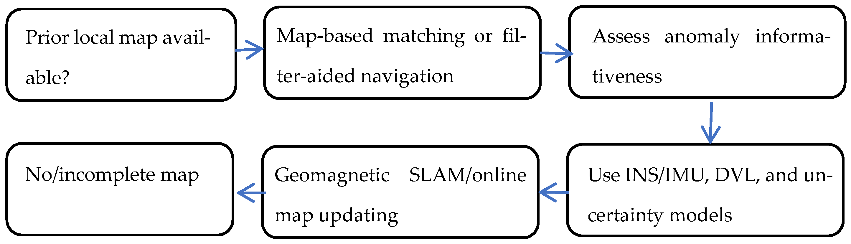
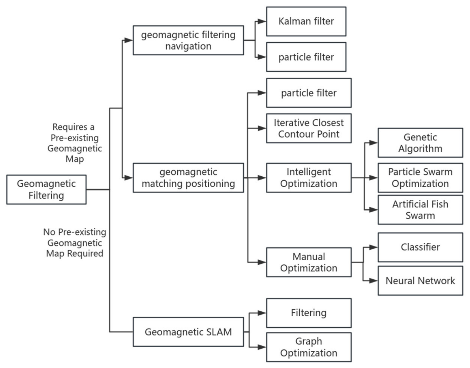
In the realm of underwater navigation, the development of reliable and accurate navigation methods is of utmost importance for various applications, such as AUV operations, underwater exploration, and marine resource surveys. With reference to the different demands on the geomagnetic reference map and the principle of positioning, the underwater geomagnetic navigation methods can be divided into three major categories in the application mode: geomagnetic matching positioning, geomagnetic filtering navigation, and geomagnetic SLAM. The decision logic for selecting an underwater geomagnetic navigation method is shown in Figure 3. Each major category is further subdivided into several specific methods, as illustrated in Figure 4.

The taxonomy in

Table 3. Problem-oriented taxonomy and critical comparison of underwater geomagnetic navigation methods.

Category	Key Assumption	Strengths	Limitations	Best Use	Representative Refs.	Data Sources	Typical Accuracy	Complexity
Map-based geomagnetic matching	Prior high-resolution magnetic map with distinctive anomalies.	Passive; interpretable; corrects INS drift.	Sensitive to map resolution, altitude mismatch, weak features and initialization error.	Surveyed routes and local inspection.	[17,20,25,28,72,73,74,75,76,77,78]	Reference map; AUV/ship/towed total-field or gradient data; INS/DVL.	Tens to hundreds of meters in informative areas; ≤100 m reported in some sea trials.	Low to moderate; window, FFT, KD-tree or multiresolution search can reduce cost.
Filter-aided geomagnetic navigation	Vehicle motion and magnetic observations can be modeled with uncertainty.	Recursive estimation; supports multi-sensor fusion.	Model mismatch, nonlinear observations, particle degeneracy and high particle cost.	Long missions with INS/DVL aiding and intermittent magnetic features.	[24,37,38,59,79,80,81,82]	Magnetometer, INS/IMU/DVL/odometry, prior map and noise models.	Suppresses INS drift; tens to hundreds of meters when the map is informative.	Moderate to high; PF cost grows with particle number.
Geomagnetic SLAM	Prior map is unavailable or incomplete; local magnetic structure can be mapped online.	Less dependent on pre-surveyed maps; useful for exploration.	Loop-closure ambiguity, sparse features, 3D mapping and scalability.	Exploration, partially mapped areas and map-updating missions.	[37,40,41,43]	Magnetic observations; INS/DVL/odometry; optional loop closure or acoustic fixes.	No common benchmark; absolute accuracy depends on anchors/loop closure.	High; graph optimization grows with pose nodes and map size.
Matching-area adaptability evaluation	Navigation should use areas with high information content and low ambiguity.	Improves route planning and reduces false matches.	Indices are dataset-specific and thresholds are not standardized.	Pre-mission route planning and map-quality assessment.	[31,32,42,83,84,85,86]	Magnetic map metrics: gradient, roughness, entropy, correlation length and ambiguity.	Not a positioning method; judged by classification accuracy and false-match risk.	Low to moderate; online evaluation is usually light.

shows that method selection should be conditioned on map availability, anomaly informativeness, vehicle dynamics, and uncertainty modeling. Consequently, a fair comparison among algorithms requires not only reporting positioning accuracy but also documenting map resolution, initialization error, sensor configuration, magnetic-interference mitigation, and computational cost.

Geomagnetic matched positioning determines an AUV’s current position by comparing real-time measured geomagnetic information with a prior geomagnetic map, assuming that the field possesses unique spatial characteristics suitable as a fingerprint for localization. Depending on sensor configuration and local observability, the prior map may record total intensity, vector components, gradients, or derived descriptors, but declination and inclination should not be assumed useful without demonstrating sufficient spatial variation and attitude accuracy [87].

Geomagnetic filtered navigation and geomagnetic SLAM both integrate matched positioning with inertial navigation to achieve continuous and stable position estimation. Filtered navigation relies on a prior map and uses algorithms such as Kalman or particle filters to fuse geomagnetic and inertial data, recursively estimating the AUV’s state (position, velocity, attitude); for example, the Extended Kalman Filter linearizes nonlinear models to enable recursive estimation. In contrast, geomagnetic SLAM collects geomagnetic and INS information frame by frame and performs frame-to-frame matching for simultaneous localization and mapping, thereby eliminating dependence on a prior map. It constructs a local map while estimating the vehicle’s position, and through continuous map and state updates, it effectively expands navigational applicability, even in areas where the prior map is inaccurate or unavailable [37].

3.1. Principle of Geomagnetic Matching-Based Localization

The working principle of geomagnetic matching navigation involves three steps: first, a high-resolution geomagnetic reference map is constructed by collecting and storing characteristic data (intensity, gradient, direction) within a predetermined navigation area; second, as the carrier (e.g., an AUV) traverses the area, an onboard magnetometer continuously records real-time geomagnetic parameters; third, a matching algorithm compares the real-time data with the reference map to identify the best match and determine the carrier’s real-time coordinates [72]. This process relies on three critical elements: a high-accuracy geomagnetic database, advanced measurement technology using high-sensitivity magnetometers, and robust matching algorithms that account for environmental disturbances and measurement uncertainties.

Current research on geomagnetic matching and positioning has reached a relatively mature stage, with algorithms classified into four main categories based on feature methods: correlation-based matching, terrain-matching-derived techniques, gravity or other geophysical matching, and methods inspired by image or signal processing. In summary, the integration of a high-quality database, precise measurement, and sophisticated algorithms is essential, and continued refinement of these components is key to enhancing accuracy, reliability, and applicability in diverse underwater environments [88].

3.2. Geomagnetic Matching-Based Localization Algorithms

3.2.1. Correlation-Based Geomagnetic Matching

Methods based on correlation analysis employ correlation criteria to quantify the degree of alignment between a measurement sequence and any subsequence within the reference map, thereby determining the positional information of the matching sequence [74]. The correlation criterion can be conceptualized as a cost function that evaluates the alignment between real-time measurements and the reference data [19]. Based on this principle, geomagnetic matching algorithms are primarily classified into three categories [19,74,75,76].

The first category comprises similarity-based algorithms, which measure the resemblance between the measurement sequence and the reference subsequence using metrics such as the Cross-Correlation Coefficient, Correlation Coefficient, Product Correlation, and Normalized Product Correlation; these methods seek to maximize the cost function, with the optimal match corresponding to its maximum value [74]. The second category consists of difference-based algorithms, which evaluate the degree of divergence using metrics like Mean Absolute Difference, Mean Square Difference, Absolute Difference, and Squared Difference, and aim to minimize the cost function [75]. The third category employs the Hausdorff Distance as a similarity metric, which measures the maximum distance between two point sets and is particularly useful for sequences with nonlinear or complex patterns; like difference-based methods, it seeks to minimize the distance to identify the best match [76]. Thus, similarity-based algorithms maximize while difference-based and Hausdorff-based algorithms minimize the cost function, a distinction that is critical for algorithm selection based on application requirements.

Internationally, the concept of Magnetic Contour Matching (MAGCOM) navigation was first proposed in the 1960s, but experimental verification was not feasible at the time due to insufficient measured geomagnetic data [20,77,78,89]. It was not until 1974–1976 that the former Soviet Union’s Ramenskoye Company successfully conducted experiments with the MAGCOM system using real data, thereby validating the concept [79]. In China, significant progress emerged later; in 2004, Li Sumin et al. from the China Aerospace Academy III applied the MAD-based MAGCOM algorithm to ground-measured magnetic data at 50-metre resolution, demonstrating terrestrial feasibility [77].

More recently, deep learning approaches have been explored. Tan et al. employed a neural network to train on seafloor point clouds, achieving superior alignment accuracy over baseline methods [90]; Yingying Wang et al. proposed an underwater data association method using variational autoencoders with a semantic segmentation module, reaching a recall rate of 92.31% [91]; and Barros et al. introduced AttDLNet, an attention-based network for 3D point cloud alignment originally designed for LiDAR, which extracts robust descriptors for high matching performance [92]. Despite their high accuracy, these deep learning methods often suffer from low computational efficiency and lack interpretability, which has revived interest in traditional correlation methods that offer greater transparency and efficiency in certain scenarios. For example, Yunfei Guo conducted a comparative analysis of four correlation methods for downhole autonomous navigation, highlighting the importance of method selection based on the specific geomagnetic environment and system requirements [93].

Correlation-based algorithms, including similarity-based, difference-based, and Hausdorff-distance variants, each have unique strengths, and the choice depends on the desired balance between accuracy, efficiency, and interpretability. Their integration with machine learning holds promise for further improvement. Critically, however, correlation methods should not be presented as universally robust; their reliability depends on sequence length, map resolution, trajectory geometry, and the uniqueness of local magnetic signatures. Future studies should report false-match rates and ambiguity metrics, not only average positioning errors.

3.2.2. Geomagnetic Matching Algorithm Based on Terrain Matching, Gravity Matching and Other Geophysical Related Techniques

The principle of geomagnetic matching shares a conceptual foundation with traditional terrain and gravity matching, as all rely on extracting and processing geophysical features to identify the optimal position. Many early geomagnetic algorithms were therefore adapted from terrain matching methods, most notably the TERCOM algorithm developed by British Aerospace, which has well-established applications in navigation systems [25,94,95]. Other similar methods include LACOM, RACOM, and SAMSOM. Their fundamental principle is that, after an initial INS position estimate, a series of sequences parallel to the projected trajectory are generated and evaluated as matching candidates. However, their efficacy depends heavily on INS accuracy and reference map quality, and they typically require a straight-line trajectory, limiting maneuverability; as a result, their localization accuracy and stability are relatively weak, especially in dynamic or complex environments [96].

To address these limitations, Zheng Hui et al. developed a SITAN method based on Multiple Model Adaptive Estimation and applied it to two western Pacific areas with prominent gravimagnetic features, demonstrating the feasibility of gravity and geomagnetic filtering-aided navigation for submarines [96]. Similarly, Bishop explored an algorithm using gravitational maps [97]. In geomagnetic matching specifically, Zhao Jianhu et al. integrated a Hausdorff-distance-based matching criterion into TERCOM with rotational transformations, significantly improving underwater matching accuracy and reliability [25]. Shengping Wang et al. combined TERCOM with the Iterative Closest Contour Point algorithm, which not only improved accuracy but also accelerated computational efficiency for real-time applications [78].

The development of geomagnetic matching algorithms has been heavily influenced by terrain and gravity techniques, and while traditional methods like TERCOM have laid the groundwork, their limitations have spurred more sophisticated approaches. Innovations such as Hausdorff-distance integration, MMAE-based SITAN, and TERCOM-ICCP hybridization have significantly enhanced performance. Critically, however, terrain- and gravity-aided analogies provide useful templates, but underwater geomagnetic navigation has different observability and disturbance characteristics. Directly transferring TERCOM or SITAN logic without considering magnetic-vector measurement uncertainty, towing geometry, and depth-dependent anomaly attenuation can lead to over-optimistic conclusions.

3.2.3. Geomagnetic Matching Algorithm Based on Image Processing, Signal Processing and Other Related Technologies

Image processing and signal processing algorithms have been increasingly integrated into geomagnetic matching navigation, significantly enhancing performance and robustness. Notable examples include the Iterative Closest Point (ICP) algorithm, the Iterative Closest Contour Point (ICCP) algorithm, the Differential ICCP (DICCP), and methods based on geomagnetic information entropy [19,72,73,74,75,76]. These originally image-oriented techniques have been adapted to address challenges such as noise reduction, error correction, and improved matching accuracy.

The ICP algorithm, proposed by Besl and McKay [98] and refined by Chen and Medioni [99] and Zhang [100], is a quaternion-based point-set alignment method widely used in image alignment and location prediction. Its adaptability and rapid convergence have enabled successful adaptation for geomagnetic navigation, though it tends to converge to local optima in regions with minimal intensity variations, leading to non-unique solutions [95]. Improvements include Ejaz’s use of ICP for INS error correction [101]; Wu Meiping et al. enhancing ICP with RANSAC to eliminate outliers [102,103]; and Sun Xin et al. implementing an ICP-based system using geomagnetic contours as matching units [104]. The ICCP algorithm [78,105,106,107,108], which matches polygonal arc segments by selecting contour points closest to trajectory distances and incorporating compatibility constraints, improves robustness but increases computational complexity and parameter sensitivity. Extensions include Li Yuze et al. applying ICCP to INS correction [109], Zhu Hai et al. using it for submarine trajectory measurement [110], Sun Dawei adapting it for cruise missiles [111], and Xiao Shenghong introducing quadratic interpolation to improve point selection [112].

Phase correlation [113,114,115] and FFT techniques [116,117,118], widely used in scene matching, have also been incorporated to leverage frequency-domain characteristics for reducing interference noise. For example, Lv Yunxiao et al. employed Contour Constraint Matching in the air domain for preliminary trajectory determination, followed by correlation polar function analysis of frequency-domain geomagnetic spectra, though this remains computationally intensive [119]. Separately, Shi Zhiyong et al. introduced entropy-based metrics [83,84,85,86], proposing a comprehensive algorithm combining geomagnetic information entropy and difference entropy that avoids cumulative errors, offers fast computation, and exhibits strong anti-interference performance [83].

In summary, the integration of ICP, ICCP, phase correlation, FFT, and entropy-based methods has significantly advanced geomagnetic matching navigation, improving accuracy, robustness, and applicability in complex environments. However, challenges remain, including computational complexity, parameter sensitivity, and sensor precision requirements. Critically, comparison across these methods is often inconsistent because studies use different maps, trajectories, noise models, and initialization errors. A standardized benchmark that includes weak-feature, strong-anomaly, and interference-rich scenarios is needed to reveal both success and failure modes.

3.3. Filter-Aided Geomagnetic Navigation

Geomagnetic filtering is a pivotal technology for enhancing navigation accuracy and reliability, particularly in GNSS-denied environments such as underwater, urban canyons, and aerospace missions with complex electromagnetic interference. Among filtering methods, the Kalman filter (KF) is the standard optimal estimator for linear dynamic systems with Gaussian noise, operating through iterative prediction and update steps; it has been widely applied in satellite and inertial fusion. However, KF performance degrades when system nonlinearities or non-Gaussian noise are present, as is common with geomagnetic field variations.

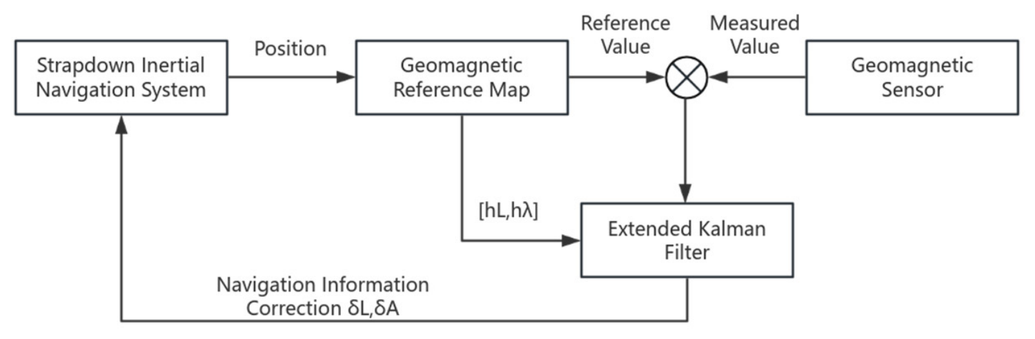
Particle filtering (PF) approximates the nonlinear Bayesian posterior and, with suitable proposal distributions and resampling strategies, can approach the minimum-mean-square-error estimate, though it suffers from computational cost, weight degeneracy, and sample impoverishment. A representative implementation is the Sandia Inertial Magnetic Aided Navigation (SIMAN) system, which integrates an IMU, a geomagnetic sensor, and a filtering-based navigation algorithm (KF or PF) to fuse continuous inertial motion data with absolute geomagnetic positional fingerprints, thereby delivering highly accurate navigation information [79]. The schematic diagram of the SIMAN algorithm is shown in Figure 5.

As described by Cheen K et al., the SIMAN system selects position and velocity errors as state vectors and formulates corresponding prediction and observation equations, which are processed by a filtering algorithm to obtain position corrections, demonstrating advantages in accuracy, stability, and real-time performance [80]. However, the strong nonlinearity of the magnetic field means that linearization in filters such as the extended Kalman filter used in SIMAN can introduce significant errors that accumulate over time, leading to filter divergence and degraded accuracy. To mitigate this, Yandeng Yang introduced an inertial/geomagnetic tight-combination navigation system based on the Unscented Kalman Filter (UKF), which uses Sigma points propagated through nonlinear equations to avoid explicit linearization, thereby improving accuracy and computational efficiency [24]. Shengping Wang et al. adopted a different strategy, using geomagnetic matching to initialize the system by comparing real-time data with pre-stored maps, which determines the linearized region’s center and size, preventing divergence and accelerating convergence [120].

Particle filtering has also been extensively applied in geomagnetic filtering for nonlinear localization problems. Xie HW et al. proposed the MaLoc method, which uses position and heading as particles, with weights determined by differences in consecutive magnetic field measurements and their probability distribution; through resampling, this method achieved positioning accuracy of 1 to 2.8 m [121]. However, particle-filter-based methods can encounter divergence with continuity changes in geomagnetic distribution [122]. Improvements have focused on motion, measurement, and weight update models: Xie HW et al. proposed dynamic step-length estimation to enhance the motion model, achieving 1 to 2 m accuracy after filtering [123]; in 2016, the U.S. Air Force Institute of Technology incorporated the Earth’s magnetic anomaly field as observational information using high-resolution USGS aerial maps, achieving an RMS error of 21.51 m at 500 m altitude; and Canciani A et al. improved the weight update model by using geomagnetic information to eliminate invalid particles, reducing maximum localization error to below 1.5 m with a 53.33% probability of achieving 1-metre accuracy [124].

In conclusion, the development of KF, PF, and their variants has significantly advanced navigation, with improvements to systems like SIMAN enhancing accuracy, reliability, and application scope. Future research may focus on further optimizing algorithms, integrating new sensors, and exploring innovative data-fusion techniques for more accurate geomagnetic-aided inertial navigation in complex environments. Critically, filtering frameworks are attractive for AUV navigation because they naturally integrate INS, DVL, acoustic, and geomagnetic measurements, but their weakness is that the observation model is usually nonlinear, map-dependent, and spatially nonuniform. Therefore, future filter designs should explicitly model map uncertainty, magnetic measurement covariance, and outlier rejection instead of relying only on nominal sensor noise.

3.4. Geomagnetic SLAM

Geomagnetic positioning technology is a sophisticated method of navigation and localization that capitalizes on the unique properties of the Earth’s magnetic field. As described in the previous section, the geomagnetic filtering and geomagnetic matching methods typically necessitate the prior construction of an accurate magnetic field map. However, in scenarios where a pre-established magnetic field map is absent, geomagnetic SLAM technology emerges as a crucial solution. Geomagnetic SLAM allows the carrier, such as an unmanned aerial vehicle (UAV), a mobile robot, or an underwater vehicle, to concurrently determine its own position and construct a magnetic field map during movement, thereby realizing autonomous localization and navigation [125].

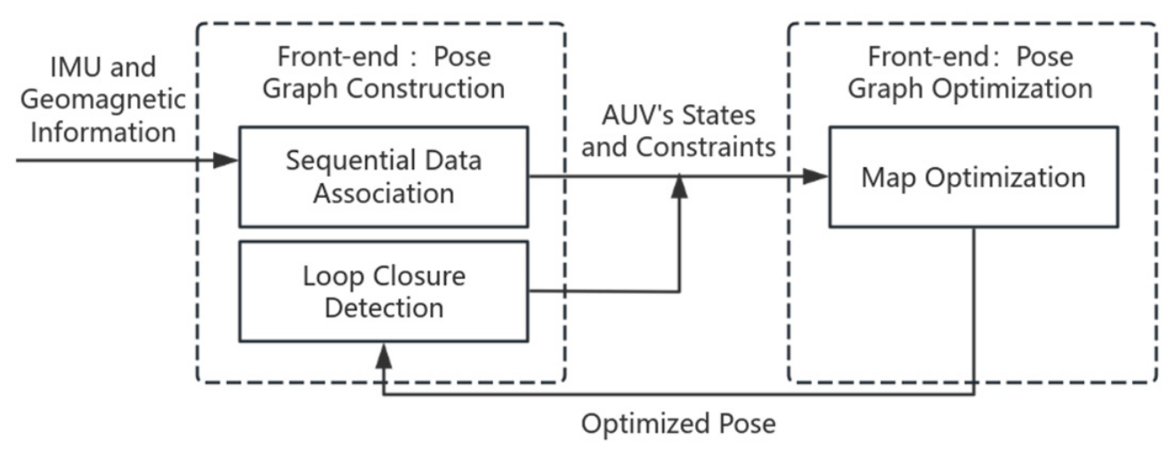
As illustrated in Figure 6, the geomagnetic SLAM technique typically follows a sequential pipeline. It begins with sensor information reading, collecting data from magnetometers (magnetic field strength and direction) and inertial sensors (acceleration and angular velocity from an IMU). Based on the carrier’s motion characteristics, a motion model (e.g., a kinematic model for wheeled robots) is established to predict future positions and orientations. A critical step is loopback detection, which identifies when the carrier has returned to a previously visited location, enabling correction of accumulated localization and mapping errors. Once loopbacks are detected, an optimization procedure (using least-squares or other algorithms) adjusts the pose estimates to minimize the discrepancy between predicted and measured values. Finally, as the carrier moves and more data are collected, a magnetic field map is constructed, which can be grid-based or feature-based and serves as a reference for subsequent navigation.

In addition to these general SLAM steps, the magnetic sensors are individually and robustly coupled with the IMU to compensate for IMU drift. By measuring the actual geomagnetic field direction and fusing it with inertial data through Kalman filtering, the system significantly improves attitude estimation accuracy [126]. This coupling is essential for maintaining reliable performance in dynamic environments.

Geomagnetic SLAM techniques can be classified into two main categories based on their underlying estimation frameworks.

The first category comprises filtering-based methods, which estimate the carrier’s position and attitude while simultaneously constructing a magnetic field map. For example, the approach described in reference [127] employs a particle filter to represent the posterior state distribution as a set of weighted particles, combined with Gaussian process regression to model the magnetic field, enabling efficient localisation and mapping using only magnetic and odometry information. The second category consists of graph-optimisation-based methods, which, after detecting loop closures, adjust graph vertices through least-squares iterative optimisation to minimise errors. Common edge constraints include odometry and loop-closure constraints, while additional constraints on magnetic features have also been introduced [128]. In graph-based SLAM, carrier poses and landmark positions are represented as vertices, and constraints as edges; optimising the graph enhances localisation and mapping accuracy.

To enhance the localization and geomagnetic map accuracy of geomagnetic SLAM, researchers have carried out in-depth studies in the following areas:

Selection of observational information: The choice of magnetic eigenquantities suitable for the specific scenario of use is crucial. For example, the reference [129] takes into account the characteristics of magnetic measurements of aerial vehicles. Aerial vehicles may encounter different magnetic field environments during flight, and by selecting appropriate magnetic features, the accuracy of localization can be improved. In addition, reference [130] explores the use of artificial magnetic beacons as wayfinding beacons underwater, which provides a new way for underwater navigation in areas with complex magnetic field conditions.

Loopback detection method: The SLAM method heavily relies on loopback detection to correct the position and map. Reference [129] performs positional relationship detection by setting the trigger radius. When the distance between the current position and a previously visited position is within the trigger radius, a loopback may be detected. On the other hand, references [128,131] perform loopback detection by calculating the similarity of magnetic sequences. By comparing the magnetic field sequences measured at different times, the system can determine whether the carrier has returned to a previously visited location.

Optimization strategy development: After detecting a loopback, an appropriate optimization strategy is essential for improving the accuracy of localization and geomagnetic map construction. Iterative optimization methods mentioned in the literature include generic graph optimization [132], network optimizer [133], stochastic gradient descent [134], and so on. These optimization methods can adjust the carrier’s pose and the magnetic field map to reduce the accumulated errors and improve the overall accuracy of the SLAM system.

These research advances demonstrate that geomagnetic SLAM technology holds great potential and application value for mapless localisation, particularly in aviation and underwater environments where GNSS signals may be disrupted or electromagnetic wave penetration is limited, making it suitable for autonomous navigation and mapping of underwater vehicles.

Critically, however, geomagnetic SLAM is promising but its maturity is lower than that of map-dependent matching. The key unresolved issues include magnetic-feature repeatability, reliable loop-closure detection in 3D underwater motion, scalable map representation, and the coupling between magnetic observations and vehicle attitude errors. Claims of map-free navigation should therefore be supported by long-range field trials and open datasets.

4. Development Trends and Critical Challenges

Since its inception at the end of the 20th century, underwater geomagnetic navigation technology has experienced a significant and gradual evolution. Initially, the focus was on theoretical exploration, where researchers delved into the fundamental principles and feasibility of using the Earth’s magnetic field for underwater navigation. Over time, this foundational knowledge led to advancements in algorithm development and optimization, enabling more accurate and reliable navigation solutions. The technology also expanded from relying solely on geomagnetic data to integrating multiple sources of information, such as acoustic signals, inertial measurements, and other environmental data, thereby enhancing the robustness and precision of the navigation system. Furthermore, it has progressed from primarily addressing static environments, where the magnetic field remains relatively stable, to effectively coping with dynamic interferences, such as those caused by underwater currents, man-made structures, and other sources of magnetic anomalies. This evolution reflects the continuous efforts to improve the adaptability and effectiveness of underwater geomagnetic navigation in various complex scenarios.

4.1. From Basic Theory to Algorithm Innovation

4.1.1. Early Theoretical Foundation (Before 2008)

The geomagnetic navigation technology was initially inspired by terrestrial terrain matching and aerial magnetic navigation. In 2008, Hao Yanling and colleagues systematically analyzed the feasibility of underwater geomagnetic matching for the first time, pointing out that the core challenges lie in the insufficient accuracy of geomagnetic maps and the impact of interfering magnetic fields. They proposed two technical approaches: the first is to eliminate local magnetic anomalies through wavelet multi-scale filtering and match them with the global geomagnetic model; the second is to use the SLAM algorithm to achieve autonomous navigation by leveraging the characteristics of geomagnetic anomalies. This stage clarified the key issues that need to be addressed in underwater geomagnetic navigation and laid the foundation for subsequent research [135].

4.1.2. Algorithm Optimization and Model Construction (2010–2015)

After 2010, the research focus of underwater geomagnetic navigation shifted to algorithm improvement and local geomagnetic field modeling. The ICCP (Iterative Closest Point) algorithm became mainstream, and Zhao Jianhu et al. optimized the local geomagnetic field accuracy through multi-surface function modeling. Experiments showed that the matching error is positively correlated with the background field accuracy (for every 1 nT increase in background field error, the matching error increases by 0.5 to 1 m) [136]. The TERCOM (Terrain Contour Matching) algorithm was also improved by introducing the Hausdorff distance criterion and adaptive rotation angle optimization, enhancing the positioning accuracy to the hundred-meter level [30]. Additionally, there was a breakthrough in potential field continuation technology, where the potential field integral iteration method extended the underwater magnetic field from airborne survey data, solving the instability issue of the traditional Fourier transform method [71].

4.1.3. Anti-Interference and Dynamic Environment Algorithms (2015–2020)

In response to the complex underwater environment, the research focus has shifted towards dynamic interference compensation. Particle filtering and Monte Carlo methods have been applied to non-Gaussian noise environments, effectively addressing the issues of accumulated errors in inertial navigation and the instability of magnetometer attitudes [40]. Meanwhile, bio-inspired navigation algorithms have emerged. Inspired by biological navigation, Liu Mingyong et al. proposed evolutionary gradient search and heading compensation strategies, which effectively counteract the trajectory drift caused by ocean currents [30,137].

4.2. From Single Scenarios to Multi-Platform Integration

Early underwater geomagnetic navigation research focused on passive stealth navigation for submarines, with Cai Zhaoyun et al. (2007) emphasizing the need for high-precision geomagnetic models and anti-interference algorithms to enable autonomous positioning [138]. With the increasing use of AUVs in marine resource exploration, the combination of geomagnetic and inertial navigation has become mainstream; Song Baowei (2022) reviewed geomagnetic navigation practices on AUVs such as the “Jiaolong” and identified a precision bottleneck at the semi-physical simulation stage (hundred-meter level), proposing multi-sensor fusion as a solution [139]. Bio-inspired navigation has also been applied to AUVs, as exemplified by Li Hong (2025), who achieved dynamic heading correction through ocean current kinematics modelling [30].

The trend towards multi-source integration and miniaturization has been reinforced by Wu Zhitian (2012) development of strapdown triaxial magnetometer attitude calibration, which significantly improves measurement accuracy [140]. The fusion of geomagnetism and RFID was successfully demonstrated by Wang Jinhua (2018), achieving meter-level positioning in mines and expanding application scenarios in complex environments [141]. Furthermore, Yang Yuanxi (2017) advanced the integration of gravity, geomagnetism and sonar, proposing a seamless underwater multi-sensor navigation system that drives the development of integrated equipment [142].

4.3. Core Technical Challenges

Early efforts to improve prior geomagnetic map accuracy were hampered by low resolution (50-metre grids), which caused underwater matching errors exceeding 500 metres [143]. Subsequent advances using high-precision magnetometer arrays [144] and optimised regularisation parameters [145] improved model accuracy to within 5 nT and reduced positioning errors to the hundred-metre level. These developments, together with existing geomagnetic instruments and maps, have provided strong technical support for marine geomagnetic matching, ensuring its feasibility [135]. For dynamic interference compensation, ocean current impacts were addressed by Li Hong (2025), who established AUV kinematic equations and estimated current velocity to achieve trajectory correction, with simulations showing a 70% reduction in drift error [30]. Similarly, Liu Mingyong (2015) designed a dynamic correction filter that maintains positioning stability even during geomagnetic storms [29].

Real-time performance and computational bottlenecks remain significant challenges. The particle filter, commonly used for non-Gaussian state estimation in nonlinear systems, requires up to 50,000 samples for convergence, imposing a heavy computational load. Future directions may include the application of deep learning algorithms to optimise geomagnetic matching and dynamically filter interference signals, as well as the introduction of edge computing technology to enable real-time underwater geomagnetic navigation.

4.4. Summary of Development Patterns

4.4.1. The Evolutionary Process of Technology

The development patterns of underwater geomagnetic navigation technology can be summarized as “demand-driven algorithm iteration, interdisciplinary breakthroughs to overcome bottlenecks, and multi-source integration to expand application scenarios.” In the future, continuous breakthroughs are needed in three aspects: real-time modeling, lightweight algorithms, and robust anti-interference capabilities, to achieve the leap from “laboratory validation” to “global ocean application.”

Table 4. Representative Technological Milestones.

Stage	Key Technological Breakthroughs	Core Contributions
Theoretical foundation period	Feasibility Analysis of Geomagnetic Matching	Proposed application path for SLAM algorithm
Algorithm optimization period	Improvement of ICCP and TERCOR	Local modeling accuracy enhanced to 5 nT
Dynamic-environment response	Bio-inspired Navigation and Particle Filtering	Ocean current compensation, non-Gaussian noise suppression
System-integration period	Multi-sensor Fusion (Geomagnetic-Inertial-RFID)	Achieved applications in multiple scenarios such as mines and AUVs
Forward-looking Exploration Period	Deep Learning and Real-time Continuation Algorithms	Addressed computational power bottlenecks and model updating issues

illustrates the representative developmental phases of underwater geomagnetic navigation technology.

4.4.2. The Evolutionary Path of Technology

In the evolution of underwater navigation technology, the algorithm layer has progressed from traditional matching algorithms (such as ICCP and TERCOR) to bio-inspired and intelligent algorithms (such as particle filtering and evolutionary search), and ultimately to multi-source fusion algorithms (such as the integration of geomagnetic, inertial, and gravity data). The model layer has evolved from global geomagnetic models to high-resolution local models and further to dynamically updated real-time models. The application layer has expanded from submarine stealth navigation to AUV ocean exploration, and then to complex environments involving multiple platforms (such as mines and polar regions). This developmental trajectory reflects the trend of advancing from basic to advanced technologies and from single-source to multi-source approaches, laying a solid foundation for the widespread application of underwater navigation technologies.

In the process of technological development, demand-driven progress and technological breakthroughs have been mutually reinforcing. On the one hand, the military’s need for stealth has propelled early research, while the demand for civilian ocean development has facilitated the practical application of the technology. On the other hand, interdisciplinary integration has emerged as a significant driving force for technological breakthroughs. The introduction and integration of geophysics (potential field continuation), bionics (mechanisms of biological navigation), and artificial intelligence (deep learning) have collectively propelled technological advancements in this field.

4.4.3. Future Development Trends

In the key directions for future technological development, the construction of high-precision geomagnetic reference maps is crucial, with sub-hundred-meter resolution and real-time updating capabilities forming the basis for precise navigation [139,142]. Meanwhile, the development of intelligent anti-interference algorithms has also become a priority. By integrating reinforcement learning to achieve environment-adaptive navigation, these algorithms can effectively cope with the complex and variable underwater environment [30]. Additionally, advancements in miniaturized sensor technology have brought breakthroughs to this field. The integration of magnetometers and inertial units not only enhances measurement accuracy but also significantly reduces the payload of AUVs, providing strong support for the efficient operation of underwater vehicles [40].

5. Discussion and Future Perspectives

The preceding review indicates that the central challenge of underwater geomagnetic navigation is not the absence of algorithms, but the mismatch between algorithmic assumptions and underwater operating conditions. Many studies demonstrate feasibility in localized or well-surveyed regions, yet fewer provide transferable evidence across depth, speed, vehicle type, magnetic cleanliness, reference-map resolution, and geomagnetic anomaly richness. Future work should therefore prioritize reproducible datasets, uncertainty-aware benchmarks, and field experiments that report not only final positioning error but also map resolution, sensor configuration, initialization error, computational load, and failure cases.

For reference management, all in-text citations should be checked against the final reference list, and every cited source should include complete bibliographic information according to the target SCI journal style. Particular attention should be paid to author spelling, year consistency, journal title capitalization, volume/issue/page information, DOI availability, and the removal of duplicate or weakly related references.

5.1. Improvement of Geomagnetic Matching Algorithms

The current geomagnetic matching algorithms still have deficiencies in complex environments. Future research can be approached from three aspects: First, develop more advanced algorithms, such as those based on deep learning. By training with a large amount of geomagnetic data, these algorithms can automatically learn the complex patterns of geomagnetic features, thereby improving matching accuracy. Second, in response to interference sources in underwater environments, such as marine organisms and seabed minerals, study matching algorithms with strong anti-interference capabilities, like adaptive filtering techniques, to achieve real-time identification and suppression of interference signals and enhance the reliability of matching. Finally, conduct research on multi-source data fusion matching by integrating geomagnetic data with data from other navigation sensors, such as acoustic and gravity sensors. Utilize multi-sensor data fusion algorithms (such as Kalman filtering and particle filtering) to achieve synergistic matching of multi-source data, including geomagnetic, acoustic, and gravity data, fully leveraging the advantages of various types of information to further improve the accuracy and reliability of navigation.

5.2. Construction and Updating of Geomagnetic Reference Maps

To better meet the navigation needs of underwater vehicles, efforts should be made in three areas: First, the creation of high-precision geomagnetic reference maps. Existing geomagnetic reference maps still have room for improvement in terms of precision and resolution. By using high-precision geomagnetic measurement equipment and advanced data processing techniques, higher-precision and higher-resolution geomagnetic reference maps can be produced, providing a more accurate reference for geomagnetic matching. Second, the establishment of a dynamic updating mechanism. Since the geomagnetic field is dynamically changing, it is necessary to continuously monitor the geomagnetic field to obtain real-time changes and promptly update the geomagnetic reference maps to ensure their timeliness and accuracy. Third, the expansion of coverage. The current coverage of geomagnetic reference maps is limited, especially in remote seas and deep ocean areas. Therefore, it is essential to further expand the coverage to meet the navigation requirements of underwater vehicles worldwide.

5.3. Enhancement of Sensor Technology

To enhance the performance of underwater magnetic navigation, efforts need to be made in three areas: First, develop high-precision, high-sensitivity magnetometers. As the core sensors for underwater magnetic navigation, their precision directly affects navigation performance. They can more accurately measure the subtle changes in the geomagnetic field, thereby improving navigation accuracy. Second, research more effective sensor calibration methods and error compensation techniques to address the impacts of various factors such as temperature, pressure, and magnetic interference that magnetometers experience during use. This will reduce measurement errors and enhance the precision and stability of the sensors. Finally, achieve multi-sensor integration by combining magnetometers with other sensors, such as inertial sensors and acoustic sensors. By working together through data fusion technology, these sensors can complement each other’s advantages, improving the overall performance and reliability of the navigation system.

5.4. Selection and Optimization of Matching Areas

To enhance the performance of underwater navigation, research needs to be conducted in three areas: feature extraction and matching area identification, optimization strategies for matching areas, and collaborative navigation using multiple matching areas. First, more effective feature extraction methods should be developed to automatically identify areas with rich geomagnetic features, thereby improving the accuracy and efficiency of matching area selection. For example, machine learning algorithms, such as principal component analysis and neural networks, can be used to extract and identify features from geomagnetic data and automatically select matching areas. Second, based on the mission requirements and environmental conditions of underwater vehicles, optimization strategies for matching areas should be developed to dynamically adjust the scope and position of matching area selection. Factors such as the vehicle’s speed, heading, and seafloor topography should be considered to choose the optimal matching area and enhance navigation performance. Finally, in some complex missions, multiple matching areas may need to work together. Therefore, collaborative navigation technology using multiple matching areas should be studied to enable information sharing and collaborative matching among these areas, further improving the accuracy and reliability of navigation.

5.5. Integration with Other Navigation Technologies

To enhance the performance of underwater navigation, geomagnetic navigation can be integrated with other navigation technologies. First, by combining geomagnetic navigation with an inertial navigation system, the long-term stability of geomagnetic navigation can be used to correct the cumulative errors of inertial navigation, thereby improving the accuracy and reliability of navigation. Second, integrating geomagnetic navigation with sonar navigation can compensate for the limitations that sonar navigation may encounter in the underwater acoustic channel, leveraging the strengths of both to further improve navigation precision and reliability. Finally, when underwater vehicles are on the water surface or near the surface, integrating them with satellite navigation systems can enable rapid positioning and updates of navigation information, thereby enhancing the overall performance of the navigation system.

5.6. Bionic Navigation Technology Research

By conducting in-depth research on the navigation mechanisms of marine organisms, such as the principles by which dolphins and sharks use the geomagnetic field for navigation, new ideas and methods can be provided for underwater geomagnetic navigation. For example, studying the magnetic induction organs and neural signal processing mechanisms of these organisms can explore their applications in geomagnetic navigation. Based on these biological navigation mechanisms, bionic navigation algorithms can be developed to simulate the navigation behaviors of these organisms, thereby improving the performance of underwater magnetic navigation. For instance, bionic algorithms such as ant colony optimization and particle swarm optimization can be used to achieve path planning and target localization in magnetic navigation. Additionally, designing bionic sensors to simulate the magnetic induction capabilities of biological organisms can enhance the performance and sensitivity of sensors. For example, developing bionic magnetometers based on the principles of biological magnetic induction can improve the accuracy and resolution of geomagnetic field measurements.

5.7. Adaptability to Underwater Complex Environments

To enhance the performance of underwater magnetic navigation systems in complex marine environments, research needs to be conducted in three areas. First, the characteristics of high pressure, low temperature, and darkness in the deep-sea environment pose higher demands on magnetic navigation systems. Therefore, it is necessary to study the adaptability of the system in the deep-sea environment, including the pressure tolerance, temperature tolerance, and anti-interference capabilities of sensors, in order to improve its working performance in the deep sea. Second, complex seafloor topography can interfere with geomagnetic signals, thereby affecting navigation accuracy. Thus, geomagnetic navigation methods under complex seafloor topography need to be studied, such as terrain-aided navigation technology that combines seafloor topographic information and geomagnetic information, to improve the accuracy and reliability of navigation. Finally, the marine environment is dynamically changing, with factors such as ocean currents and tides affecting geomagnetic signals. Therefore, the adaptability of geomagnetic navigation systems in a dynamic marine environment also needs to be studied to ensure their stable operation under constantly changing conditions.

5.8. System Integration and Application Verification

System integration and optimization, application validation and testing, as well as standardization and regulation are key elements in enhancing the performance of underwater magnetic navigation systems. First, by integrating geomagnetic navigation systems with other navigation systems, control systems, etc., and by researching system integration architectures and interface designs, seamless connections and collaborative operations between different systems can be achieved, thereby optimizing the overall performance of the system. Second, application validation and testing on actual underwater vehicles, through extensive experiments and tests, continuously improve the design and optimize the system to assess its performance and reliability, and enhance its practicality and reliability. Finally, establishing technical standards, testing standards, data formats, and other standard specifications for underwater magnetic navigation systems can help promote the dissemination, application, and industrial development of this technology.

6. Conclusions

Underwater geomagnetic navigation is best understood as an end-to-end sensing, mapping, and nonlinear estimation problem. Reliable performance requires magnetic measurements whose uncertainty is small relative to local anomaly contrast; reference maps with documented spatial, temporal, and interpolation uncertainty; and algorithms selected according to map availability, observability, initialization, and computational resources. Scalar total-field measurements are operationally attractive, while vector and gradient measurements can add information when calibration and attitude accuracy are sufficient.

The literature shows promising local demonstrations but does not yet support a universal accuracy claim. Progress toward dependable long-duration AUV operation requires standardized benchmark datasets, magnetic-clean vehicle design, repeated three-dimensional surveys, explicit uncertainty budgets, false-match reporting, and sea trials that document sensor configuration, map resolution, initialization, environmental conditions, and computational cost. Multi-sensor fusion and emerging quantum magnetometers are important opportunities, but their benefit must be evaluated within this complete evidence chain.

References

1. Hasan, K.; Ahmad, S.; Liaf, A.F.; Karimi, M.; Ahmed, T.; Shawon, M.A.; Mekhilef, S. Oceanic Challenges to Technological Solutions: A Review of Autonomous Underwater Vehicle Path Technologies in Biomimicry, Control, Navigation, and Sensing. IEEE Access 2024, 12, 46202–46231. [Google Scholar] [CrossRef]
2. Li, J.; Xia, Y.; Xu, G.; Guo, Z.; Han, H.; Wu, Z.; Xu, K. Enhanced Three-Dimensional Trajectory Tracking Control for AUVs in Variable Operating Conditions Using FMPC-FTTSMC. Ocean Eng. 2024, in press. [Google Scholar] [CrossRef]
3. Salavasidis, G.; Munafò, A.; Harris, C.A.; McPhail, S.D.; Rogers, E.; Phillips, A.B. Towards Arctic AUV Navigation. IFAC-Pap. 2018, 51, 287–292. [Google Scholar] [CrossRef]
4. Mahdi, A.E.; Azouz, A.; Abdalla, A.E.; Abosekeen, A. A Machine Learning Approach for an Improved Inertial Navigation System Solution. Sensors 2022, 22, 1687. [Google Scholar] [CrossRef] [PubMed]
5. Teixeira, F.C.; Pascoal, A.M. Geophysical Navigation of Autonomous Underwater Vehicles Using Geomagnetic Information. IFAC Proc. Vol. 2008, 41, 178–183. [Google Scholar] [CrossRef]
6. Luo, Q.; Liu, B.; Yu, M.; Su, Y.; Yang, L.; Wang, L. Inertial-Geomagnetic Integrated Navigation Method Based on Kalman Filter and Adaptive Search Area. In Advances in Guidance, Navigation and Control, ICGNC 2024; Yan, L., Duan, H., Deng, Y., Eds.; Springer: Singapore, 2025; Volume 1346, pp. 462–466. [Google Scholar] [CrossRef]
7. Guo, C.; Zhang, L.; Cai, H. Analysis of Geomagnetic Navigation Accuracy under Magnetic Storms. Chin. J. Space Sci. 2011, 31, 372–377. [Google Scholar] [CrossRef]
8. Ma, X.; Zhang, J.; Li, T.; Hao, L.; Duan, H. Super-Resolution Geomagnetic Reference Map Reconstruction Based on Dictionary Learning and Sparse Representation. IEEE Access 2020, 8, 84316–84325. [Google Scholar] [CrossRef]
9. Zhou, J.; Ge, Z.; Shi, G.G.; Liu, Y.X. Development and Key Technologies of Geomagnetic Navigation. J. Astronaut. 2008, 29, 1467–1472. [Google Scholar] [CrossRef]
10. Hine, A. Magnetic Compasses and Magnetometers; Technical Report; University of Toronto Press: Toronto, ON, Canada, 1968. [Google Scholar]
11. Titterton, D.H.; Weston, J.L. Strapdown Inertial Navigation Technology, 2nd ed.; American Institute of Aeronautics and Astronautics: Reston, VA, USA, 2004. [Google Scholar]
12. Hu, X.; Wu, M. Underwater Geomagnetic Navigation Technology; National Defense Industry Press: Beijing, China, 2013. [Google Scholar]
13. Polvani, D. Magnetic Guidance of Autonomous Vehicles, Part 2. In Proceedings of the 1987 5th International Symposium on Unmanned Untethered Submersible Technology, Durham, NH, USA, 22–24 June 1987; pp. 257–264. [Google Scholar]
14. Psiaki, M.L. Autonomous Low-Earth-Orbit Determination from Magnetometer and Sun Sensor Data. J. Guid. Control Dyn. 1999, 22, 296–304. [Google Scholar] [CrossRef] [PubMed]
15. Tyrén, C. Magnetic Anomalies as a Reference for Ground-Speed and Map-Matching Navigation. J. Navig. 1982, 35, 242–254. [Google Scholar] [CrossRef]
16. Yang, Y. Research on Navigation Correction Methods for Intelligent Underwater Robots. Master’s Thesis, Harbin Engineering University, Harbin, China, 2013. [Google Scholar]
17. Wagner, C.S.; Popper, S.W. Identifying Critical Technologies in the United States: A Review of the Federal Effort. J. Forecast. 2003, 22, 113–128. [Google Scholar] [CrossRef]
18. Qiao, Y.; Wang, S.; Zhang, Q. Analysis of the Restrictive Factors of Geomagnetic Matching Guidance Technology Applied to Missile Weapon Systems. Cruise Missiles 2006, 8, 39–41. [Google Scholar]
19. Liu, Y. Research on Geomagnetic Matching Navigation Algorithm and Geomagnetic Field Simulation System. Master’s Thesis, Harbin Institute of Technology, Harbin, China, 2011. [Google Scholar]
20. Goldenberg, F. Geomagnetic Navigation beyond the Magnetic Compass. In Proceedings of the IEEE/ION Position, Location, and Navigation Symposium, Coronado, CA, USA, 25–27 April 2006; pp. 684–694. [Google Scholar] [CrossRef]
21. Kato, N.; Shigetomi, T. Underwater Navigation for Long-Range Autonomous Underwater Vehicles Using Geomagnetic and Bathymetric Information. Adv. Robot. 2009, 23, 787–803. [Google Scholar] [CrossRef]
22. Mu, H.; Wu, Z.; Wu, M. Analysis of Underwater Geomagnetic/Inertial Integrated Navigation Experiments. J. Chin. Inert. Technol. 2013, 21, 386–391. [Google Scholar]
23. Wu, Z.; Hu, X.; Wu, M.; Yan, D. An Experimental Evaluation of Autonomous Underwater Vehicle Localization on a Geomagnetic Map. Appl. Phys. Lett. 2013, 103, 104102. [Google Scholar] [CrossRef]
24. Yan, D.; Ren, J.; Song, Y. Research on Integrated Inertial/Geomagnetic Navigation Technology. Mach. Electron. 2007, 25, 19–22. [Google Scholar]
25. Zhao, J.; Liu, H.; Zhang, Y.; Wang, S. Research on Local Geomagnetic Field Modeling Method Based on Multi-Surface Functions. Mar. Sci. Bull. 2009, 28, 89–96. [Google Scholar]
26. Lin, Y. Hausdorff-Based RC and IESIL Combined Positioning Algorithm for Underwater Geomagnetic Navigation. EURASIP J. Adv. Signal Process. 2010, 2010, 593238. [Google Scholar] [CrossRef]
27. Wei, J. Current Status of Key Technologies in Geomagnetic Matching Navigation. Electron. Qual. 2017, 1, 108–110. [Google Scholar]
28. Wang, S. Research on the Technology of Marine Geomagnetic Matching Navigation and Positioning. Acta Geod. Cartogr. Sin. 2013, 42, 153. [Google Scholar]
29. Liu, M.; Li, H.; Liu, K.; Yang, P. Navigation Method of Autonomous Underwater Vehicle with Disturbance Due to Geomagnetic Anomaly Considered. J. Northwest. Polytech. Univ. 2015, 33, 627–632. [Google Scholar]
30. Li, H.; Liu, M.; Liu, K. Geomagnetic Bio-Inspired Navigation Method of AUV in the Presence of Ocean Current. Prog. Geophys. 2017, 32, 982–987. [Google Scholar] [CrossRef]
31. Chong, Y.; Chai, H.Z.; Liu, F.; Wang, X.; Du, Z.Q. Suitability Analysis of Geomagnetic Map Based on Fuzzy Decision Theory. Geomat. Inf. Sci. Wuhan Univ. 2021, 46, 118–124. [Google Scholar] [CrossRef]
32. Zhong, Y.; Chai, H.; Guo, Y.; Wang, X.; Liu, B. Matching Area Selection for AUV Geomagnetic Navigation by Self-organizing Optimization Classification. Geomat. Inf. Sci. Wuhan Univ. 2022, 47, 722–730. [Google Scholar] [CrossRef]
33. Yu, H.; Li, Z.; Yang, W.; Shen, T.; Liang, D.; He, Q. Underwater Geomagnetic Localization Based on Adaptive Fission Particle-Matching Technology. J. Mar. Sci. Eng. 2023, 11, 1739. [Google Scholar] [CrossRef]
34. Wang, B.; Huang, L.; Liu, J.; Deng, Z.; Fu, M. A Support Vector Regression-Based Integrated Navigation Method for Underwater Vehicles. IEEE Sens. J. 2020, 20, 8875–8883. [Google Scholar] [CrossRef]
35. Wei, S.; Liao, X.; Zhang, H.; Pang, J.; Zhou, Y. Recent Progress of Fluxgate Magnetic Sensors: Basic Research and Application. Sensors 2021, 21, 1500. [Google Scholar] [CrossRef] [PubMed]
36. Lühr, H.; Korte, M.; Mandea, M. The Recent Geomagnetic Field and Its Variations. In Geomagnetic Field Variations; Springer: Berlin/Heidelberg, Germany, 2009; pp. 25–63. [Google Scholar]
37. Liu, T.; Zhao, T.; Zhao, H.; Wang, C. Adaptive Cubature Kalman Filter for Inertial/Geomagnetic Integrated Navigation System Based on Long Short-Term Memory Network. Appl. Sci. 2024, 14, 5905. [Google Scholar] [CrossRef]
38. Luo, Q.; Yu, M.; Yan, X.; Zhou, Z.; Wang, C.; Liu, B. A Geomagnetic/Odometry Integrated Localization Method for Differential Robot Using Real-Time Sequential Particle Filter. Sensors 2024, 24, 2120. [Google Scholar] [CrossRef] [PubMed]
39. Ge, Z.; Zhou, J. A New Approach to Geomagnetic Matching Navigation. In Proceedings of the 2nd International Conference on Space Information Technology, Wuhan, China, 10 November 2007; SPIE-International Society For Optical Engineering: Bellingham, WA, USA, 2007; Volume 6795. [Google Scholar] [CrossRef]
40. Li, H.; Wang, G.; Li, X.; Lian, Y. A Review of Underwater SLAM Technologies. In Proceedings of the 2023 5th International Conference on Robotics, Intelligent Control and Artificial Intelligence, Hangzhou, China, 1–3 December 2023; pp. 215–225. [Google Scholar] [CrossRef]
41. Zhang, H.; Wang, Z.; Zhou, S.; Ma, C.; Wang, S.; Zhang, F.; Xu, L. Underwater Horizontal Attitude Determination Technology Based on Fusion Power Circle Theory and Improved 3D Cone Hough Transform. Electronics 2024, 13, 4689. [Google Scholar] [CrossRef]
42. Parekh, P.; Yuan, F.; Zhou, Y. Area/Power-Efficient True-Single-Phase-Clock D-Flip-Flops with Improved Metastability. In Proceedings of the 2020 IEEE 63rd International Midwest Symposium on Circuits and Systems, Springfield, MA, USA, 9–12 August 2020; pp. 182–185. [Google Scholar] [CrossRef]
43. Merveille, F.F.R.; Jia, B.; Xu, Z.; Fred, B. Advancements in Sensor Fusion for Underwater SLAM: A Review on Enhanced Navigation and Environmental Perception. Sensors 2024, 24, 7490. [Google Scholar] [CrossRef] [PubMed]
44. Pappoe, J.A.; Akimasa, Y.; Kandil, A.; Mahrous, A. Machine Learning Techniques for Estimation of Pc5 Geomagnetic Pulsations Observed at Geostationary Orbits during Solar Cycle 23. J. Atmos. Sol.-Terr. Phys. 2024, 260, 106258. [Google Scholar] [CrossRef]
45. Chung, T.K.; Kim, H.S.; Sun, C.G.; Chung, C.K. Mosaic-Based Spatial Interpolation Method Considering Topography for Subsurface Mapping Using Borehole Data in Seoul. KSCE J. Civ. Eng. 2024, 29, 100091. [Google Scholar] [CrossRef]
46. Alken, P.; Thébault, E.; Beggan, C.D.; Amit, H.; Aubert, J.; Baerenzung, J.; Bondar, T.N.; Brown, W.J.; Califf, S.; Chambodut, A.; et al. International Geomagnetic Reference Field: The Thirteenth Generation. Earth Planets Space 2021, 73, 49. [Google Scholar] [CrossRef]
47. Tang, C.; Shi, H.; Zhang, L. Geomagnetic Matching Cooperative Positioning Method for Unmanned Boat Cluster Based on Factor Graph. Ocean Eng. 2024, 296, 116901. [Google Scholar] [CrossRef]
48. Thomson, A.W.P. Improving the Modelling of the Geomagnetic Main Field: Isolating the Average Ionospheric Field in Satellite Data. Earth Planets Space 2000, 52, 1199–1206. [Google Scholar] [CrossRef]
49. Qiao, Y.; Wang, S.; Zhang, Q. Selection of Geomagnetic Matching Feature Quantities. Seismol. Geomagn. Obs. Res. 2007, 1, 42–47. [Google Scholar]
50. Qi, W.; Wang, X.; Li, X.; Liu, D. Selection of Geomagnetic Matching Feature Quantities Based on Statistical Modeling. Prog. Geophys. 2010, 25, 324–330. [Google Scholar] [CrossRef]
51. Zhou, X. Research on Underwater Geomagnetic Navigation Matching Algorithms. Master’s Thesis, Tianjin University, Tianjin, China, 2007. [Google Scholar]
52. Dang, L.; Wu, Z.; Dong, C.; Zhang, J. Data Processing Methods and Applications of Towed Marine Triaxial Magnetic Gradient Instrument. J. Mar. Sci. 2024, 42, 81–90. [Google Scholar]
53. Mu, X.; He, B.; Wu, S.; Zhang, X.; Song, Y.; Yan, T. A Practical INS/GNSS/DVL/PS Integrated Navigation Algorithm and Its Application on Autonomous Underwater Vehicle. Appl. Ocean Res. 2021, 106, 102441. [Google Scholar] [CrossRef]
54. Ma, M.; Zhou, W.; Xiu, L.; Wang, X.; Li, Y.; Li, W.; Yun, J.; Lu, Z. Fusion and Integrated Interpretation of Multisource Geoscience Datasets for Mineral Exploration. J. Appl. Geophys. 2024, 228, 105445. [Google Scholar] [CrossRef]
55. Ren, X. Design and Implementation of a Magnetic Exploration Background Field Data Processing System for UAVs. Master’s Thesis, Harbin Institute of Technology, Harbin, China, 2022. [Google Scholar]
56. Wang, Y.; Xie, C.; Liu, Y.; Zhu, J.; Qin, J. A Multi-Sensor Fusion Underwater Localization Method Based on Unscented Kalman Filter on Manifolds. Sensors 2024, 24, 6299. [Google Scholar] [CrossRef] [PubMed]
57. Li, H.; Wei, Y.; Zou, W.; Xiao, F.; Peng, X.; Qu, W. Selection of Geomagnetic Matching Feature Elements Based on IGRF13 and WMM2020 Models. Prog. Geophys. 2022, 37, 1414–1421. [Google Scholar]
58. Nie, L.; Qiu, Y.; Shen, W.; Zhang, S.; Zhang, B. Accuracy Evaluation and Applicability of IGRF12 and WMM2015 Model in Chinese Mainland. Geomat. Inf. Sci. Wuhan Univ. 2017, 42, 1229–1235, 1291. [Google Scholar]
59. Kim, D.; Bang, H.; Lee, J.C. Approach to Geomagnetic Matching for Navigation Based on a Convolutional Neural Network and Normalised Cross-Correlation. IET Radar Sonar Navig. 2019, 13, 774–782. [Google Scholar] [CrossRef]
60. Wang, Y.; Xu, Y.; An, Z. Global and China Regional Geomagnetic Reference Field Models. In Proceedings of the 6th Academic Annual Conference of the Chinese Geophysical Society; Chinese Geophysical Society: Beijing, China, 1990. [Google Scholar]
61. Ma, T.; Zhang, W.; Li, Y.; Zhao, Y.; Zhang, Q.; Mei, X.; Fan, J. Communication-Constrained Cooperative Bathymetric Simultaneous Localisation and Mapping with Efficient Bathymetric Data Transmission Method. J. Navig. 2022, 75, 1000–1016. [Google Scholar] [CrossRef]
62. Gao, J.T.; An, Z.C.; Gu, Z.W.; Zhang, Y.T. Selection of the Geomagnetic Normal Field an d Calculation of Geomagnetic Anomalous Field. Chin. J. Geophys. 2005, 48, 66–73. [Google Scholar] [CrossRef]
63. Olsen, N.; Lühr, H.; Finlay, C.C.; Sabaka, T.J.; Mandea, M.; Maus, S. The CHAOS-4 Geomagnetic Field Model. Geophys. J. Int. 2014, 197, 815–827. [Google Scholar] [CrossRef]
64. An, Z.C.; Peng, F.L.; Liu, S.H.; Wang, G.F. Inspection and Study on the Geomagnetic Survey, Charts and Models during 1683-1949 in China. Chin. J. Geophys. 2014, 57, 3795–3803. [Google Scholar]
65. An, Z.; Tan, D. Legendre Polynomial Model of the Geomagnetic Field over Eastern Asia in 1980. Acta Geophys. Sin. 1995, 38, 227–233. [Google Scholar] [CrossRef] [PubMed]
66. An, Z.C.; Rotanova, N.M. Calculations and Analyses of the Geomagnetic Field Models for East Asia. Chin. J. Geophys. 2002, 45, 34–41. [Google Scholar] [CrossRef]
67. Gu, Z.W.; An, Z.C.; Guan, J.T.; Zhang, Y.T. Spherical Cap Harmonic Analysis of the Geomagnetic Field in the Beijing-Tianjin-Hebei Region. Chin. J. Geophys. 2004, 47, 1128–1134. [Google Scholar] [CrossRef]
68. Zhao, J.; Wang, S.; Liu, H.; Zhang, Y. Establishment of a Legendre Polynomial Model for the Normal Field of Marine Local Geomagnetic Field. Prog. Geophys. 2008, 23, 1802–1808. [Google Scholar]
69. Xu, R.; Gu, Z.; Li, Z.; An, Z. Application of Geomagnetic Measurement and Geomagnetic Field Model in China from 2005 to 2010. Prog. Geophys. 2014, 29, 2092–2098. [Google Scholar]
70. Peng, F.; Xiong, L.; Chen, Y. Simulation of Geomagnetic Model Construction and Selection of Matching Feature Quantities. Autom. Instrum. 2020, 35, 87–92. [Google Scholar]
71. Wang, S.; Wang, Z.; Zhang, J.; Qiao, Y. Preparation Technology of Benchmark Maps Using Total Magnetic Field Intensity Gradient Modulus as Matching Feature Quantities. Syst. Eng. Electron. 2009, 31, 881–885. [Google Scholar]
72. Deng, C.; Huang, C.; Zhao, H.; Li, B. Review of Geomagnetic Matching Navigation Algorithms. Sci. Technol. Eng. 2012, 12, 180–186. [Google Scholar]
73. Sun, J.; Chen, J.; Deng, M. Geometric Similarity Measurement Algorithm and Experimental Analysis for Linear Spatial Data Transmission. J. Geo-Inf. Sci. 2011, 13, 701–706. [Google Scholar] [CrossRef]
74. Hu, X. Research on Geomagnetic Matching Algorithm for Underwater Navigation System. Master’s Thesis, Shandong Agricultural University, Qufu, China, 2011. [Google Scholar]
75. Liang, Y. Research on Technology of INS/Geomagnetic Matching Integrated Navigation System. Master’s Thesis, Harbin Engineering University, Harbin, China, 2010. [Google Scholar]
76. Hasan, A.M.; Samsudin, K.; Ramli, A.R.; Azmir, R.; Ismail, A.F. A Review of Navigation Systems: Integration and Algorithms. Aust. J. Basic Appl. Sci. 2009, 3, 943–959. [Google Scholar] [CrossRef]
77. Li, S.; Zhang, W. Application of Geomagnetic Field Resources in Matching Guidance. Guid. Fuzing 2004, 25, 19–21. [Google Scholar]
78. Wang, S.; Zhang, H.; Zhao, J.; Zhang, Y. Integrated Geomagnetic Matching Navigation Using TERCOM and ICCP. Geomat. Inf. Sci. Wuhan Univ. 2011, 36, 1209–1211. [Google Scholar]
79. Dai, Z.; Kang, C. Geomagnetic Field Aided Inertial Navigation Using the SITAN Algorithm. In Proceedings of the 2014 2nd International Conference on Systems and Informatics, Shanghai, China, 15–17 November 2014; pp. 79–83. [Google Scholar]
80. Chen, K.; Liang, W.C.; Liu, M.X.; Li, S. A Comparison of Geomagnetic Aided Navigation Algorithms for Hypersonics. J. Zhejiang Univ.-Sci. A 2020, 21, 673–68383. [Google Scholar] [CrossRef]
81. Stepanov, O.A.; Toropov, A.B. Nonlinear Filtering for Map-Aided Navigation. Part 1. An Overview of Algorithms. Gyroscopy Navig. 2015, 6, 324–337. [Google Scholar] [CrossRef]
82. Stepanov, O.A.; Toropov, A.B. Nonlinear Filtering for Map-Aided Navigation. Part 2. Trends in the Algorithm Development. Gyroscopy Navig. 2016, 7, 82–89. [Google Scholar] [CrossRef]
83. Shi, Z.; Xu, Y.; Wang, Y. Geomagnetic Matching Localization Algorithm Based on Entropy. Fire Control Command Control 2010, 35, 8–10. [Google Scholar]
84. Yuan, N. Research on Matching Algorithms for Terrain-Aided Navigation Systems. Master’s Thesis, Harbin Engineering University, Harbin, China, 2007. [Google Scholar]
85. Wang, H.; Yan, L.; Qian, X.; Liu, J. Comprehensive Terrain Matching Algorithm Based on Terrain Entropy and Terrain Differential Entropy. Comput. Technol. Dev. 2007, 17, 25–27. [Google Scholar]
86. Ma, H.; Liu, J.; Yang, J. Terrain Matching Algorithm Based on Terrain Entropy Difference and Elevation Absolute Difference. J. Command Technol. Inst. 2000, 11, 59–63. [Google Scholar]
87. Zhao, H.; Zhang, N.; Xu, L.; Lin, P.; Liu, Y.; Li, X. Summary of Research on Geomagnetic Navigation Technology. IOP Conf. Ser. Earth Environ. Sci. 2021, 769, 032031. [Google Scholar] [CrossRef]
88. Adkar, C.K. Magnetic Navigation System. U.S. Patent 3,728,525, 17 April 1973. [Google Scholar]
89. Miressi, M.J. Magnetic Variation: A Primitive Concept and Its Hold on Contemporary Navigation. In Proceedings of the IEEE PLANS ‘92 Position Location and Navigation Symposium, Monterey, CA, USA, 23–27 March 1992; pp. 357–361. [Google Scholar]
90. Tan, J.; Torroba, I.; Xie, Y.; Folkesson, J. Data-Driven Loop Closure Detection in Bathymetric Point Clouds for Underwater SLAM. arXiv 2022, arXiv:2209.08578. [Google Scholar]
91. Wang, Y.; Sun, Q.; Wang, Q.; Zhang, G. A Multi-AUV Cooperative Localization Method Based on Maximum Correntropy. Exp. Technol. Manag. 2022, 39, 17–23. [Google Scholar]
92. Barros, T.; Garrote, L.; Pereira, R.; Premebida, C.; Nunes, U.J. AttDLNet: Attention-Based Deep Network for 3D LiDAR Place Recognition. In Proceedings of the ROBOT2022: Fifth Iberian Robotics Conference; Springer: Cham, Switzerland, 2023; Volume 589, pp. 309–320. [Google Scholar] [CrossRef]
93. Guo, Y.; Wang, J.; Wu, B.; Zhang, L. Analysis and Optimization of Matching Algorithms for Underground Geomagnetic Positioning. Chin. J. Sens. Actuators 2018, 31, 93–98. [Google Scholar]
94. Behzad, K.P.; Benhrooz, K.P. Vehicle Localization on Gravity Maps; SPIE: Bellingham, DC, USA, 1999; Volume 3963, pp. 182–191. [Google Scholar]
95. Zhang, L.; Yang, H. Research on Combined Underwater Terrain Matching Algorithm Based on ICCP and TERCOM. J. Ballist. Guid. 2008, 28, 230–232. [Google Scholar]
96. Zheng, H.; Wang, Y.; Wang, H.; Zhao, J. Simulation Study on Aiding Underwater Submarine Navigation with the Earth’s Gravity and Magnetic Field. Geomat. Inf. Sci. Wuhan Univ. 2012, 37, 1198–1202. [Google Scholar]
97. Bishop, G.C. Gravitational Field Maps and Navigational Errors. IEEE J. Ocean. Eng. 2002, 27, 726–737. [Google Scholar] [CrossRef]
98. Besl, P.J.; McKay, N.D. A Method for Registration of 3-D Shapes. IEEE Trans. Pattern Anal. Mach. Intell. 1992, 14, 239–256. [Google Scholar] [CrossRef]
99. Chen, Y.; Medioni, G. Object Modeling by Registration of Multiple Range Images. In Proceedings of the IEEE International Conference on Robotics and Automation, Sacramento, CA, USA, 9–11 April 1991. [Google Scholar]
100. Zhang, Z. Iterative Point Matching for Registration of Free-Form Curves and Surfaces. Comput. Vis. 1994, 13, 119–152. [Google Scholar] [CrossRef]
101. Ejaz, M. Robust Geomagnetic-Aided Inertial Navigation of Underwater Vehicles Using the ICP Algorithm. In Proceedings of the 2009 Asia-Pacific Conference on Computational Intelligence and Industrial Applications, Wuhan, China, 28–29 November 2009; Volume 1, pp. 257–262. [Google Scholar]
102. Wu, M.; Liu, Y.; Hu, X. Application of the ICP Algorithm in Geomagnetic Aided Navigation. Aerosp. Control 2007, 25, 17–21. [Google Scholar]
103. Fischler, M.A.; Bolles, R.C. Random Sample Consensus: A Paradigm for Model Fitting with Application to Image Analysis and Automated Cartography. Commun. ACM 1981, 24, 381–395. [Google Scholar] [CrossRef]
104. Sun, X. Research on Magnetic Sensors Based on Giant Magnetic Impedance Effect and Geomagnetic Matching Algorithms. Master’s Thesis, Harbin Institute of Technology, Harbin, China, 2008. [Google Scholar]
105. Cordon, O.; Damas, S. Image Registration with Iterated Local Search. J. Heuristics 2006, 12, 73–94. [Google Scholar] [CrossRef]
106. Wu, H. Research on Underwater Aided Navigation Combination Method Based on Terrain Entropy and ICCP Algorithm. Ship Sci. Technol. 2011, 33, 54–57. [Google Scholar]
107. Yang, K. Research on Inertial Navigation Technology Aided by Gravity Field and Geomagnetic Field. Master’s Thesis, University of Electronic Science and Technology of China, Chengdu, China, 2006. [Google Scholar]
108. Behzad, K.P.; Behrooz, K.P. Registration Algorithms for Geophysical Maps. IEEE Ocean. Conf. 1997, 2, 974–980. [Google Scholar]
109. Li, Y.; Shi, Z.; Yang, Y. Geomagnetic Matching Localization Method Based on the ICCP Algorithm. Mod. Electron. Tech. 2008, 31, 122–124. [Google Scholar]
110. Zhu, H.; Wang, S.; Cai, P. Underwater Linear Segment Geomagnetic Matching Based on ICCP. J. Chin. Inert. Technol. 2009, 17, 153–155. [Google Scholar]
111. Sun, D.; Wang, S. Research on Cruise Navigation Geomagnetic Matching Method Based on Contour Matching. Navig. Missiles 2009, 9, 53–55. [Google Scholar]
112. Xiao, S.; Bian, S.; Huang, X. Research on Underwater Geomagnetic Correction of Inertial Navigation Using ICCP. Ship Electron. Eng. 2011, 31, 83–86. [Google Scholar]
113. Guo, Q.; Wei, R.; Hu, X.; Wu, M. Simulation Study of Geomagnetic Matching Dual-Contour Algorithm. J. Syst. Simul. 2010, 22, 1576–1579. [Google Scholar]
114. Kobayashi, K.; Nakajima, H.; Aoki, T.; Matsumoto, S. Principles of Phase-Only Correlation and Applications. ITE Tech. Rep. 1996, 20, 1–6. [Google Scholar]
115. Morikawa, M.; Katsumata, A.; Higuchi, T.; Sato, K. An Image Processor Implementing Algorithms Using Characteristics of Phase Spectrum of Two-Dimensional Fourier Transformation. In Proceedings of the IEEE International Symposium on Industrial Electronics, Bled, Slovenia, 12–16 July 1999; Volume 3, pp. 120–1213. [Google Scholar]
116. Wu, S.; Fu, Y.; Deng, H. Real-Time Image Matching System Based on Phase Correlation Algorithm. Comput. Simul. 2005, 22, 84–86. [Google Scholar]
117. Srinivasa, R.B.; Chatter, B.N. An FFT-Based Technique for Translation-, Rotation-, and Scale-Invariant Image Registration. IEEE Trans. Image Process. 1996, 5, 1266–1271. [Google Scholar] [CrossRef] [PubMed]
118. Harold, S.S.; Robert, W. Blind Cross-Spectral Image Registration Using Prefiltering and Fourier-Based Translation Detection. IEEE Trans. Geosci. Remote Sens. 2002, 40, 637–650. [Google Scholar] [CrossRef]
119. Lv, Y.; Chen, Q.; Zhang, W.; Shi, Z. Frequency-Domain Correlation Geomagnetic Matching Algorithm Based on Geomagnetic Signal Features. J. Chin. Inert. Technol. 2010, 18, 580–584. [Google Scholar]
120. Wang, S.; Zhao, J.; Wu, Z. Research on the Key Technology of Marine Geomagnetic Matching Navigation and Positioning; China University of Geosciences Press: Beijing, China, 2017. [Google Scholar]
121. Xie, H.W.; Gu, T.; Tao, X.P.; Lu, J.; Niu, W. MaLoc: A Practical Magnetic Fingerprinting Approach to Indoor Localization Using Smartphones. In Proceedings of the ACM International Joint Conference on Pervasive and Ubiquitous Computing, Seattle, WA, USA, 13–17 September 2014. [Google Scholar]
122. Li, W.; Huang, H.; Luo, D. Indoor Geomagnetic Matching Accuracy Analysis Based on Improved Particle Filter Algorithm. Sci. Surv. Mapp. 2018, 43, 109–114. [Google Scholar]
123. Xie, H.W.; Gu, T.; Tao, X.P.; Lu, J.; Niu, W. A Reliability-Augmented Particle Filter for Magnetic Fingerprinting Based Indoor Localization on Smartphones. IEEE Trans. Mob. Comput. 2015, 15, 1877–1892. [Google Scholar] [CrossRef]
124. Canciani, A.; Raguet, J. Absolute Positioning Using the Earth’s Magnetic Anomaly Field. Navigation 2016, 63, 111–126. [Google Scholar] [CrossRef]
125. Zhang, Q.; Li, Y.; Ma, T.; Cong, Z.; Zhang, W. Bathymetric Particle Filter SLAM with Graph-Based Trajectory Update Method. IEEE Access 2021, 9, 85464–85475. [Google Scholar] [CrossRef]
126. Viset, F.; Helmons, R.; Kok, M. An Extended Kalman Filter for Magnetic Field SLAM Using Gaussian Process Regression. Sensors 2022, 22, 2833. [Google Scholar] [CrossRef] [PubMed]
127. Vallivaara, I.; Haverninen, J.; Kemppainen, A.; Koskinen, J. Simultaneous Localization and Mapping Using Ambient Magnetic Field. In Proceedings of the 2010 IEEE Conference on Multisensor Fusion and Integration, Salt Lake City, UT, USA, 5–7 September 2010; pp. 14–19. [Google Scholar]
128. Joongdae, J.; Taekjun, O.; Hyun, M. Magnetic Field Constraints and Sequence-Based Matching for Indoor Pose Graph SLAM. Robot. Auton. Syst. 2015, 70, 92–105. [Google Scholar] [CrossRef]
129. Lee, T.N.; Canciani, A.J. MagSLAM: Aerial Simultaneous Localization and Mapping Using Earth’s Magnetic Anomaly Field. Navigation 2020, 67, 95–107. [Google Scholar] [CrossRef]
130. Chang, S.; Fu, X.; Zhang, C.; Zhao, Y.; Du, X. An Underwater SLAM Approach Using Magnetic Beacons. J. Unmanned Undersea Syst. 2019, 27, 277–283. [Google Scholar]
131. Chao, G.; Harlle, R. Sequence-Based Magnetic Loop Closures for Automated Signal Surveying. In Proceedings of the 2015 International Conference on Indoor Positioning and Indoor Navigation, Banff, AB, Canada, 13–16 October 2015; pp. 1–12. [Google Scholar]
132. Kümmerle, R.; Grisetti, G.; Strasdat, H.; Konolige, K.; Burgard, W. G2o: A General Framework for Graph Optimization. In Proceedings of the 2011 IEEE International Conference on Robotics and Automation, Shanghai, China, 9–13 May 2011; pp. 3607–3613. [Google Scholar] [CrossRef]
133. Woolfram, B.; Oliver, B.; Cyrill, S. A Tree Parameterization for Efficiently Computing Maximum Likelihood Maps Using Gradient Descent. In Robotics: Science and Systems III; MIT Press: Cambridge, MA, USA, 2008; pp. 65–72. [Google Scholar]
134. Olson, E.; Leonard, J.; Teller, S. Fast Iterative Alignment of Pose Graphs with Poor Initial Estimates. In Proceedings of the 2006 IEEE International Conference on Robotics and Automation, Orlando, FL, USA, 15–19 May 2006; pp. 2262–2269. [Google Scholar]
135. Hao, Y.; Zhao, Y.; Hu, J. Preliminary Analysis on the Application of Geomagnetic Field Matching in Underwater Vehicle Navigation. Prog. Geophys. 2008, 23, 594–598. [Google Scholar]
136. Zhao, J.; Zhang, H.; Wang, A.; Liu, H. Underwater Geomagnetic Navigation Based on ICCP. Geomat. Inf. Sci. Wuhan Univ. 2010, 35, 261–264. [Google Scholar]
137. Guo, J.; Liu, M.; Liu, K.; Niu, Y.; Wang, M. Research of Bio-Inspired Geomagnetic Navigation for AUV Based on Evolutionary Gradient Search. J. Northwest. Polytech. Univ. 2019, 37, 865–870. [Google Scholar] [CrossRef]
138. Cai, Z.; Wei, H.; Ren, Z. A Review of Underwater Geomagnetic Navigation Technology. Natl. Def. Sci. Technol. 2007, 3, 28–29. [Google Scholar]
139. Song, B.W.; Pan, G.; Zhang, L.; Wang, Y.H.; Mao, Z. Development Trend and Key Technologies of Autonomous Underwater Vehicles. Chin. J. Ship Res. 2022, 17, 27–44. [Google Scholar]
140. Wu, Z.T.; Wu, Y.X.; Hu, X.P.; Wu, M.P. Calibration of Strapdown Three-axis Magnetometer and Measurement Error Compensation of Geomagnetic Field Based on Total Least Squares. Acta Armamentarii 2012, 33, 1202–1209. Available online: https://kns.cnki.net/kcms2/article/abstract?v=KXYaOrH3lTmtZXQvuksrXSjrWOHhKrSdFZ5JRVzR3Lm-KatJ6nAZxivpjBREKElgWoWIdjAfaxx2JHqMGc5umo-PuOx4w8jlKoYvzcUto-qb8jYYoQuAn1p7sBTqL5Tyx5wlRmujFitot7iIS5Zp-bOtUbsqg2TFHc-e7QYAyq9DP6fErvi4KA==&uniplatform=NZKPT&language=CHS (accessed on 29 July 2026).
141. Wang, J.H.; Li, W.Q.; Chen, X.T.; Guo, Y.F. Algorithm Research and Simulation Experiment of Underground Positioning with GRPM. J. China Coal Soc. 2018, 43, 338–343. [Google Scholar] [CrossRef]
142. Yang, Y.; Xu, T.; Xue, S. Progresses and Prospects in Developing Marine Geodetic Datum and Marine Navigation of China. Acta Geod. Cartogr. Sin. 2017, 46, 1–8. [Google Scholar]
143. Zhao, L.; Yan, T.J. Positioning Performance Evaluation of Magnetic Contour Matching under Different Accuracy of Sensor. Acta Phys. Sin. 2013, 62, 067702. [Google Scholar] [CrossRef]
144. Zhang, X.J.; Kang, X.Y.; Fan, L.M.; Zheng, Q.; Chen, X.; Kang, C. The Method of the Magnetic Object Locating by Arrays in the Geomagnetic Total Field. Chin. J. Geophys. 2019, 62, 1921–1928. [Google Scholar] [CrossRef]
145. Ma, T.; Chen, L.; Wu, M.; Hu, X. Selection of Regularization Parameter in Downward Continuation of Potential Field Based on L-Curve Method. Prog. Geophys. 2013, 28, 2485–2494. [Google Scholar]
Figure 1. End-to-end sensing, mapping, and estimation chain for underwater geomagnetic navigation.
Jmse 14 01447 g001
Figure 2. Schematic diagram of the magnetic field of a geocentric dipole.
Jmse 14 01447 g002
Figure 3. Decision logic for selecting an underwater geomagnetic navigation method.
Jmse 14 01447 g003
Figure 4. Classification of the geomagnetic localization methods.
Jmse 14 01447 g004
Figure 5. Schematic of the SIMAN algorithm.
Jmse 14 01447 g005
Figure 6. Process of the geomagnetic SLAM algorithm.
Jmse 14 01447 g006