Robust Adaptive Propagated Interval Observer for Actuator Fault Diagnosis in Underactuated AUVs

Abstract

This paper presents an interval-observer-based actuator fault detection and isolation (FDI) method for underactuated autonomous underwater vehicles (AUVs) under bounded hydrodynamic uncertainty and time-varying ocean currents. A locally frozen linear time-invariant (LTI) representation enables deterministic set-membership analysis, and the robust adaptive propagated interval observer (RAPIO) propagates admissible center–radius state bounds within a Lyapunov framework. Adaptivity is introduced through a reinforcement learning (RL)-augmented uncertainty-bound modulation mechanism, where an offline-trained agent scales a nonnegative channel-wise slack term without modifying the scheduled observer-gain rule or the nominal center predictor. Under the stated observer and disturbance-envelope conditions, positivity, stability, and diagnostic-channel inclusion hold for any bounded learning signal. Actuator loss-of-effectiveness (LoE) faults are represented through the actuator-effectiveness channel and detected through interval-consistency violations, enabling axis-wise isolation of surge, yaw-rate, and pitch-rate actuator faults. The same schedule-blind decision layer is additionally evaluated with structurally distinct additive-bias and stuck/jam actuator models. All stuck/jam events are detected, and bias-magnitude sweeps identify channel-wise 100%-detection boundaries with zero false alarms. A structured 72-case scenario sweep shows reliable detection, strong false-alarm rejection, and acceptable detection delays compared with benchmark observers.

1. Introduction

AUVs have become essential platforms for deep-sea surveys, offshore inspections, and environmental monitoring, where human access is difficult or impossible [1]. However, the performance of these platforms can degrade under strong ocean disturbances and hydrodynamic parameter uncertainties because of the nonlinear added-mass and damping coefficients [2]. Furthermore, in underactuated configurations, limited redundancy and nonlinear coupling amplify these vulnerabilities, and actuator faults such as loss of effectiveness, bias, or jamming can lead to mission failure [3]. Therefore, autonomous, long-duration AUV missions require an integrated fault-tolerant control architecture with a reliable fault detection and isolation (FDI) module [4,5].

In the FDI literature, model-based approaches remain the preferred choice for safety-critical marine applications due to their analytical transparency and formal guarantees [6]. Among these, observer-based techniques are particularly attractive due to their minimal computational demand and structural simplicity [7]. Nevertheless, classical observers such as extended Kalman filters (EKF) and fixed-threshold residual generators are often sensitive to modeling mismatch and external disturbances, which may result in unreliable decisions [8,9].

Set-membership and interval-based observers address these limitations by treating violations of admissible state bounds as deterministic fault indicators [10,11]. Unlike stochastic filters, interval observers propagate bounded uncertainty directly and detect faults through interval-consistency violations [10,12]. For nonlinear AUV dynamics, locally frozen LTI and LPV-inspired representations enable tractable observer synthesis while retaining operating-point dependence [13,14,15]. Similar linearization strategies have also been used for underwater, aerial, and ground-vehicle FDI [16]. Related set-membership developments include ellipsoidal reachability for nonlinear robust FDI [17], unknown-input interval observers [18], and distributed interval/unknown-input observers [19]. However, these methods still rely on fixed or structurally prescribed uncertainty descriptions, limiting their response to time-varying hydrodynamic conditions. Because worst-case uncertainty bounds are selected offline, this fixed-bound assumption—common in interval-observer FDI—can reduce detection performance when operating conditions change [20]. Zonotopic set-membership FDI under event-triggered communication shows the value of bounded-set estimation in multi-agent systems [21], but it still assumes static or slowly varying bound structures. Zhu et al. [22] reduce conservatism using a fixed-gain LPV interval observer bank with offline $H^{-}/H_{\infty }$ LMI optimization and an open-loop boundary update indexed by a slowly varying scheduling parameter. This improves mild operating-point variation, but the update does not use runtime residual feedback and can therefore mismatch randomized hydrodynamic disturbances outside the scheduling grid. Convex/polytopic LPV observers similarly offer certificate-oriented synthesis, but their prescribed scheduling structure and direct fault-reconstruction objective do not address residual-adaptive bounded-set consistency under time-varying AUV hydrodynamic and current uncertainty [23].

Stochastic robust filters provide another route. The robust EKF of Song and He [24] models environmental perturbations as multiplicative process noise and evaluates a normalized innovation against a calibrated scalar threshold, but one design-time threshold cannot both suppress Coriolis-induced cross-channel residuals in healthy operation and retain sensitivity to small actuator faults. Online sign-based adaptive interval observers [25] replace conservative constants with sign-based adaptive parameters driven by measurement consistency. Their interval width adapts online, but the sign-based law can lag rapidly varying Coriolis-coupled disturbances, increasing detection delay and false alarms under strong hydrodynamic uncertainty.

To provide greater adaptability, data-driven and reinforcement-learning (RL) approaches have been explored [26,27]. However, when learning is embedded directly into observer gains or residual thresholds, interval inclusion and stability may be compromised. Any resulting guarantee may hold only after the policy has converged and while operation remains within its training distribution, a condition that cannot be assured during deployment in unknown marine environments [28].

The observer design problem has also been studied extensively for fractional-order systems. Observer-based model-reference control for linear fractional-order systems has been developed using Caputo derivatives, Lyapunov analysis, and LMI tools [29,30]. Nonlinear extensions include Hadamard fractional-order one-sided Lipschitz observer/controller design [31], unknown-input observer synthesis for generalized proportional fractional-order systems [32], and practical observers for state and sensor-fault reconstruction [33]. These works address fractional-order dynamics beyond the present integer-order AUV model. Even so, their rigorous observer architectures support the broader principle used here: the learning or adaptation mechanism should be separated from the core observer dynamics to preserve formal guarantees under uncertainty.

These studies leave four linked limitations. Fixed-bound interval observers [16,20] cannot react to real-time residual feedback outside the offline design envelope. LPV/$H^{-}/H_{\infty }$ adaptive methods [22] use open-loop scheduling whose certificates do not cover residual-feedback or learned modulation signals. Stochastic robust filters [24] and sign-based adaptive observers [25] rely on scalar thresholds or lagging adaptation laws. As a result, it is difficult to reject channel-specific false alarms while retaining sensitivity to small faults. RL-assisted methods [26,28] close the adaptation loop, but often place the policy inside the observer core. This makes stability and inclusion conditional on policy convergence.

Accordingly, AUV FDI requires residual-feedback adaptation. Such adaptation should preserve formal inclusion and stability independently of learning convergence. It should also provide channel-specific alarm modulation without changing the observer gains. The novelty of RAPIO is the separation between the certified observer and the learned adaptation signal. Unlike fixed or adaptive interval/set-membership observers whose bounds are prescribed offline, RAPIO updates the admissible tube using runtime residual information. The update is also not tied to an offline scheduling grid, as it would be under LPV/$H^{-}/H_{\infty }$ boundary scheduling. Crucially, it does not alter the scheduled observer-gain rule, nominal center predictor, or residual maps directly. The observer gain-scheduling rule remains fixed, so analytical stability and interval inclusion remain independent of policy convergence under the stated observer and disturbance-envelope assumptions, including out-of-distribution bounded policy outputs.

The main contributions of this work are as follows:

• An RL-augmented RAPIO architecture is developed in which the frozen SAC policy modulates only bounded tube slack; the observer gains, center predictor, and detector thresholds remain fixed.
• A locally frozen LTI interval observer is formulated for the underactuated AUV, with Metzler/Hurwitz certification and componentwise inclusion on the diagnostic channels ${\mathcal{I}}_d=\{u,r,q\}$.
• An interval-consistency rule combines leaky bound-excess accumulation, confirmation/recovery gates, and center freezing for surge, yaw, and pitch isolation. The same schedule-blind detector identifies additive bias and stuck/jam faults without metadata.
• A structured 72-case scenario sweep benchmarks RAPIO against an adaptive interval observer and a P2P threshold FDI method, showing $100\%$ detection on all channels with zero event-level false alarms.

The remainder of this paper is organized as follows. Section 2 gives the formulation of the actuator FDI problem and introduces the system model. Section 3 presents the interval-observer-based FDI approach. It includes observer design, stability properties, and axis-wise fault isolation. Section 4 gives the details of the simulation setup and Section 5 reports the results and comparative analyses. Section 6 discusses the principal findings and trade-offs. Finally, Section 7 concludes the paper.

2. Problem Formulation

To formulate robust interval-based fault diagnosis under bounded uncertainty, we first state the assumptions governing the AUV dynamics and operating environment.

Assumption 1

([34,35]). The AUV dynamics satisfy the nonlinear fault-affected model given in (1).

$$\dot{\mathit{x}}\left(t\right)=f\left(\mathit{x}\left(t\right),\mathit{u}\left(t\right)\right)+\mathit{d}\left(t\right)+\mathit{F}{\mathit{f}}_a\left(t\right),$$

(1)

where $\mathit{x}\left(t\right)\in {\mathbb{R}}^{12}$ is the system state, $\mathit{u}\left(t\right)\in {\mathbb{R}}^3$ is the augmented actuator command, $f\left(·\right)$ is locally Lipschitz, $\mathit{d}\left(t\right)$ denotes bounded disturbances encompassing ocean current effects and hydrodynamic uncertainty, and ${\mathit{f}}_a\left(t\right)$ represents unknown additive actuator fault effects entering the state dynamics through a known distribution matrix $\mathit{F}\in {\mathbb{R}}^{12\times 3}$. In this work, the augmented command is $\mathit{u}={[{\delta }_s,{\delta }_r,n]}^{\top }$, where the TNMPC optimizes the stern-plane and rudder deflections ${[{\delta }_s,{\delta }_r]}^{\top }\in {\mathbb{R}}^2$ and a separate RPM loop generates the propeller speed n. Throughout the manuscript, $n_x:=12$ denotes the state dimension. The unbold symbol n in the actuator command is reserved for propeller rotational speed (RPM).

Assumption 2.

Let $\mathit{\rho }\left(t\right)\in {\mathbb{R}}^{n_{\rho }}$ denote the vector of scheduling variables (a measurable subset of the state and/or input, e.g., $\mathit{\rho }\left(t\right)=\rho \left(\mathit{x}\right(t),\mathit{u}(t\left)\right)$) used to parameterize the locally frozen linear model matrices $\mathit{A}\left(\mathit{\rho }\right(t\left)\right)$ and $\mathit{B}\left(\mathit{\rho }\right(t\left)\right)$. The scheduling variables satisfy

$$\parallel \mathit{\rho }\left(t\right)-\mathit{\rho }\left(t_k\right)\parallel \le {\epsilon }_{\rho },t\in [t_k,t_{k+1}),$$

(2)

for some ${\epsilon }_{\rho }>0$.

Moreover, the system operates inside compact admissible sets ${\mathcal{X}}_c\subset {\mathbb{R}}^{12}$ and ${\mathcal{U}}_c\subset {\mathbb{R}}^3$ such that $\mathit{x}\left(t\right)\in {\mathcal{X}}_c$ and $\mathit{u}\left(t\right)\in {\mathcal{U}}_c$ for all admissible missions. The admissible sampled command profile is bounded and rate-limited on each diagnostic interval. Saturations, command holds, and actuator-mode changes are treated as sampled inputs. Their residual effect on the frozen model is included in the calibrated disturbance budget. Let $\mathit{z}\left(t\right)={[{\mathit{x}}^{\top }\left(t\right),{\mathit{u}}^{\top }\left(t\right)]}^{\top }$. The diagnostic sampling instants satisfy $t_{k+1}=t_k+T_s$, where $T_s>0$ is the diagnostic update period. Over ${\mathcal{Z}}_c={\mathcal{X}}_c\times {\mathcal{U}}_c$, the nonlinear dynamics $f(\mathit{x},\mathit{u})$ are twice continuously differentiable and there exists a constant $L_{\Delta }>0$ such that

$$\parallel \Delta \left(t\right)\parallel \le L_{\Delta }{\parallel \mathit{z}\left(t\right)-\mathit{z}\left(t_k\right)\parallel }^2,t\in [t_k,t_{k+1}),$$

(3)

where $\Delta \left(t\right)$ denotes the higher-order Taylor remainder. The compact-set condition is required only in the fault-free case; during a fault the true state may exit the interval, which is precisely the detection mechanism.

Remark 1.

Assumption 2 defines a local validity envelope for the frozen model, not a global linear approximation. On the compact set ${\mathcal{Z}}_c$, bounded and rate-limited admissible trajectories admit finite rate bounds ${\overline{v}}_x$, ${\overline{v}}_u$, ${\overline{v}}_{\rho }$, defined by $\parallel \dot{\mathit{x}}\left(t\right)\parallel \le {\overline{v}}_x$, $\parallel \dot{\mathit{u}}\left(t\right)\parallel \le {\overline{v}}_u$, and $\parallel \dot{\mathit{\rho }}\left(t\right)\parallel \le {\overline{v}}_{\rho }$ on ${\mathcal{Z}}_c$, giving $\parallel \mathit{\rho }\left(t\right)-\mathit{\rho }\left(t_k\right)\parallel \le {\overline{v}}_{\rho }{T}_s$ and $\parallel \mathit{z}\left(t\right)-\mathit{z}\left(t_k\right){\parallel }^2\le ({\overline{v}}_x^2+{\overline{v}}_u^2)T_s^2$. Substituting into (3) and letting ${\overline{r}}_i={\overline{\tilde{d}}}_i-{\overline{d}}_i^{\mathrm{phys}}>0$ denote the available componentwise residual margin, a sufficient sampling condition for keeping the Taylor remainder inside the disturbance envelope is

$$T_s\le min\left\{{\displaystyle \frac{{\epsilon }_{\rho }}{{\overline{v}}_{\rho }}},\sqrt{{\displaystyle \frac{{\displaystyle \underset{i}{min}{\overline{r}}_i}}{L_{\Delta }({\overline{v}}_x^2+{\overline{v}}_u^2)}}}\right\}.$$

(4)

Here, ${\overline{d}}_i^{\mathrm{phys}}$ is the componentwise bound allocated to the physical disturbance and frozen-point offset before the Taylor-remainder budget is added, and ${\overline{\tilde{d}}}_i$ is the corresponding aggregate bound defined in (21). If (4) is violated in a new operating regime, inclusion must be restored by reducing $T_s$, refreezing the Jacobian more frequently, or enlarging $\overline{\tilde{\mathit{d}}}$.

Assumption 3.

The disturbance $\mathit{d}\left(t\right)$ satisfies the componentwise bounds in (5):

$$\underline{\mathit{d}}\le \mathit{d}\left(t\right)\le \overline{\mathit{d}},\forall t\ge 0,$$

(5)

where $\underline{\mathit{d}},\overline{\mathit{d}}\in {\mathbb{R}}^{12}$ are known constant vectors corresponding to the full velocity–kinematic state dimension. In practice, the velocity-channel bounds are derived from ocean-current models. In the simulations of Section 4, currents up to $0.3$ m/s enter through ${\mathit{M}}^{-1}{\mathit{\tau }}_d$. The kinematic states are not directly forced in the lumped disturbance representation of (12); their uncertainty is propagated through the velocity and attitude dynamics.

2.1. Nonlinear AUV Dynamics with Actuator Faults

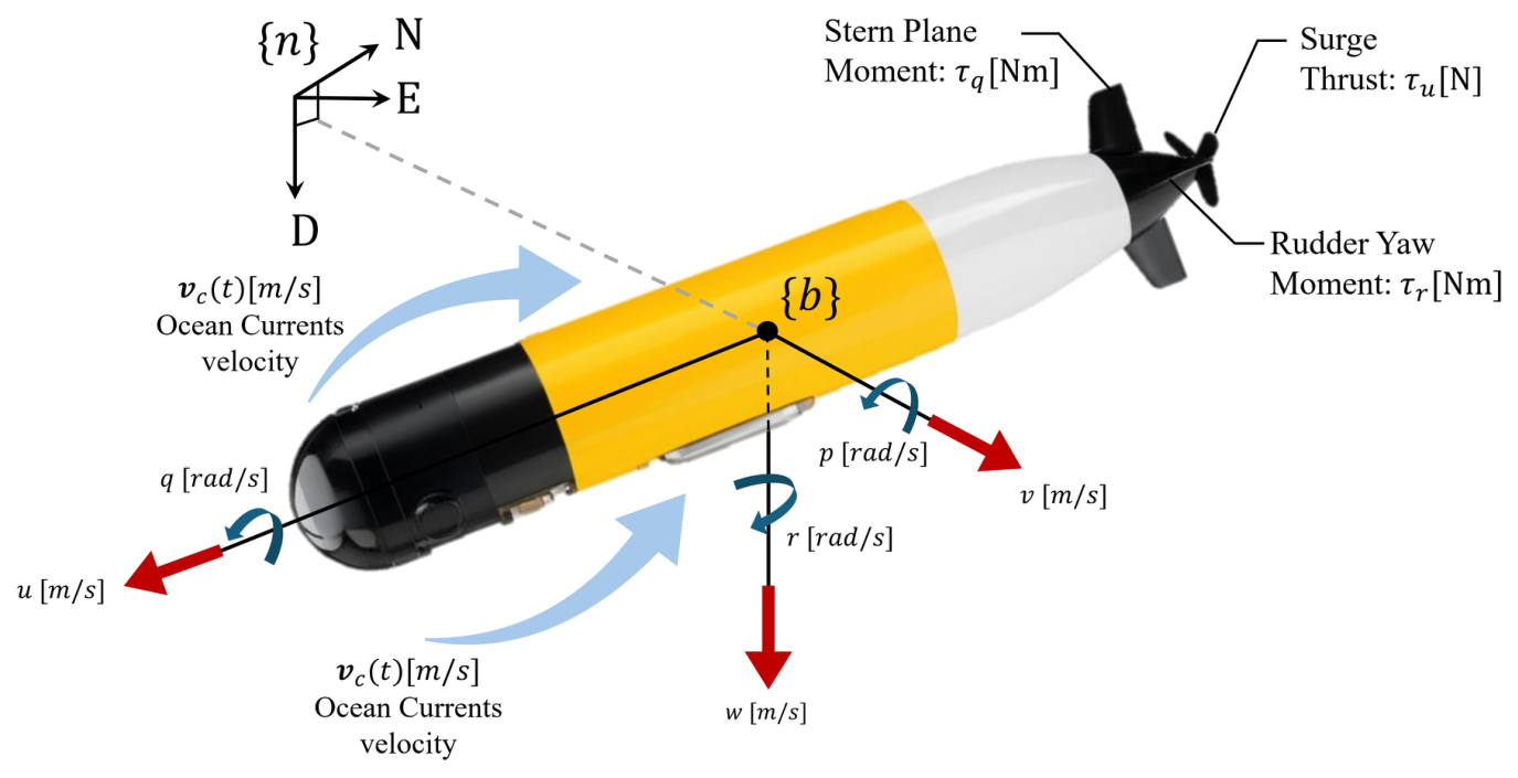
The AUV motion is described in a body-fixed frame $\left\{b\right\}$ and an inertial North–East–Down (NED) frame $\left\{n\right\}$, as shown in Figure 1. Body-fixed velocities u, v, and w denote surge, sway, and heave, respectively, and p, q, and r denote roll, pitch, and yaw rates. The inertial coordinates x, y, and z denote North, East, and Down position, while $\varphi$, $\theta$, and $\psi$ are the roll, pitch, and yaw Euler angles, respectively. The vehicle is actuated in surge by propulsion force ${\tau }_u$, in yaw by control moment ${\tau }_r$, and in vertical motion by stern-plane force ${\tau }_w$, which affects both heave and pitch. Ocean current effects are modeled as an unknown bounded disturbance $\mathit{d}\left(t\right)$ consistent with Assumption 3.

The body-fixed velocity and inertial position–orientation vectors are defined in (6):

$$\mathit{\nu }={\left[\begin{array}{cccccc}u& v& w& p& q& r\end{array}\right]}^{\top },\mathit{\eta }={\left[\begin{array}{cccccc}x& y& z& \varphi & \theta & \psi \end{array}\right]}^{\top }.$$

(6)

The nonlinear 6-DOF AUV dynamics are

$$\begin{array}{cc}\hfill \mathit{M}\left(\mathit{\nu }\right)\dot{\mathit{\nu }}+\mathit{C}\left(\mathit{\nu }\right)\mathit{\nu }+\mathit{D}\left(\mathit{\nu }\right)\mathit{\nu }+\mathit{g}\left(\mathit{\eta }\right)& =\mathit{\tau }+{\mathit{\tau }}_d,\hfill \\ \hfill \dot{\mathit{\eta }}& =\mathit{J}\left(\mathit{\eta }\right)\mathit{\nu },\hfill \end{array}$$

(7)

The kinematic transformation in (7) maps the body-fixed translational and angular velocities into NED position and Euler-angle rates. For the adopted 3–2–1 yaw–pitch–roll convention, the transformation is given by (8):

$$\mathit{J}\left(\mathit{\eta }\right)=\left[\begin{array}{cc}{\mathit{R}}_b^n(\varphi ,\theta ,\psi )& {\mathbf{0}}_{3\times 3}\\ {\mathbf{0}}_{3\times 3}& \mathit{T}(\varphi ,\theta )\end{array}\right],$$

(8)

where the blocks in (9) use $c_{\chi }=cos\chi$ and $s_{\chi }=sin\chi$:

$${\mathit{R}}_b^n=\left[\begin{array}{ccc}{c}_{\psi }{c}_{\theta }& c_{\psi }{s}_{\theta }{s}_{\varphi }-s_{\psi }{c}_{\varphi }& c_{\psi }{s}_{\theta }{c}_{\varphi }+s_{\psi }{s}_{\varphi }\\ s_{\psi }{c}_{\theta }& s_{\psi }{s}_{\theta }{s}_{\varphi }+c_{\psi }{c}_{\varphi }& s_{\psi }{s}_{\theta }{c}_{\varphi }-c_{\psi }{s}_{\varphi }\\ -s_{\theta }& c_{\theta }{s}_{\varphi }& c_{\theta }{c}_{\varphi }\end{array}\right],\mathit{T}=\left[\begin{array}{ccc}1& s_{\varphi }tan\theta & c_{\varphi }tan\theta \\ 0& c_{\varphi }& -s_{\varphi }\\ 0& s_{\varphi }/c_{\theta }& c_{\varphi }/c_{\theta }\end{array}\right],$$

(9)

where, ${\mathit{R}}_b^n\in {\mathbb{R}}^{3\times 3}$ rotates a vector from the body frame to NED, and $\mathit{T}\in {\mathbb{R}}^{3\times 3}$ maps the body angular-rate vector ${[p,q,r]}^{\top }$ to ${[\dot{\varphi },\dot{\theta },\dot{\psi }]}^{\top }$. The Euler representation is used over the regular operating set $\left|\theta \right|<\pi /2$, for which $c_{\theta }\ne 0$ and $\mathit{T}$ is nonsingular. In (7), $\mathit{M}\left(\mathit{\nu }\right)$ is the inertia matrix including added-mass effects, $\mathit{C}\left(\mathit{\nu }\right)$ denotes Coriolis and centripetal terms, $\mathit{D}\left(\mathit{\nu }\right)$ represents nonlinear hydrodynamic damping, $\mathit{g}\left(\mathit{\eta }\right)$ collects the hydrostatic restoring forces and moments, $\mathit{\tau }\in {\mathbb{R}}^6$ is the generalized control input, and ${\mathit{\tau }}_d\in {\mathbb{R}}^6$ represents external disturbances.

The underactuated actuator map is nonlinear in the augmented command and is written as (10):

$$\mathit{\tau }={\mathit{\tau }}_{\mathrm{nom}}(\mathit{x},\mathit{u})+{\mathit{\tau }}_f(\mathit{x},\mathit{u},\mathit{\alpha }),$$

(10)

where $\mathit{u}={[{\delta }_s,{\delta }_r,n]}^{\top }$ collects stern-plane deflection, rudder deflection, and propeller RPM, and $\mathit{\alpha }={[{\alpha }_u,{\alpha }_s,{\alpha }_r]}^{\top }$ denotes the actuator effectiveness factors for surge propulsion, stern planes, and rudder. The additive term ${\mathit{\tau }}_f$ is therefore an equivalent local force/moment difference induced by the multiplicative LoE model used by the plant, not an independently injected state offset.

Expanding (7) yields the componentwise velocity dynamics in (11):

$${\dot{\nu }}_i={\displaystyle \frac{1}{m_i}}\left({\mathcal{F}}_i\left(\mathit{\nu }\right)+{\tau }_i+{\tau }_i^f+d_i\right),$$

(11)

where $m_i$ is the effective inertia (including added mass), ${\mathcal{F}}_i\left(\mathit{\nu }\right)$ aggregates the nonlinear hydrodynamics, ${\tau }_i$ and ${\tau }_i^f$ are the nominal and fault-induced inputs, and $d_i$ represents the bounded disturbance in channel i. The index $i\in \{1,\dots ,6\}$ follows the generalized force ordering (surge, sway, heave, roll, pitch, yaw).

For interval-based diagnosis, the physical disturbance is represented as (12),

$$\mathit{d}\left(t\right)=\left[\begin{array}{c}{\mathit{M}}^{-1}\left(\mathit{\nu }\left(t\right)\right){\mathit{\tau }}_d\left(t\right)\\ {\mathbf{0}}_{6\times 1}\end{array}\right]\in {\mathbb{R}}^{12},$$

(12)

where the lower zero block reflects that the kinematic states are not directly driven by external forces. Ocean current effects appearing in $\dot{\mathit{\eta }}=\mathit{J}\left(\mathit{\eta }\right)\mathit{\nu }$ enter through the relative-velocity terms embedded in $\mathit{C}\left(\mathit{\nu }\right)$ and $\mathit{D}\left(\mathit{\nu }\right)$.

Combining the above yields the compact nonlinear state-space model

$$\dot{\mathit{x}}\left(t\right)=f(\mathit{x}\left(t\right),\mathit{u}\left(t\right))+\mathit{d}\left(t\right)+{\mathit{F}}_{\mathrm{phys}}(\mathit{x},\mathit{u}){\mathit{f}}_a\left(t\right),$$

(13)

with state ordering $\mathit{x}={[u,v,w,p,q,r,x,y,z,\varphi ,\theta ,\psi ]}^{\top }$. Now, at the physical actuator level, let ${\mathit{f}}_a={[\Delta T,\Delta Z_s,\Delta Y_r]}^{\top }$ collect the fault-induced changes in propeller thrust, stern-plane vertical force, and rudder lateral force. For the actuator geometry used in the nonlinear plant,

$${\mathit{\tau }}_f={\mathit{B}}_f^{\mathrm{eq}}{\mathit{f}}_a,{\mathit{B}}_f^{\mathrm{eq}}=\left[\begin{array}{ccc}1& 0& 0\\ 0& 0& 1\\ 0& 1& 0\\ 0& 0& 0\\ 0& L_s& 0\\ 0& 0& L_r^{*}\end{array}\right],$$

where stern-plane LoE gives $\Delta Z_s=({\alpha }_s-1)Z_{uuds}{u}^2{\delta }_s$ and $\Delta M_s=({\alpha }_s-1)Z_{uuds}{u}^2{\delta }_s{L}_s$, rudder LoE gives $\Delta Y_r=({\alpha }_r-1)Y_{uudr}{u}^2{\delta }_r$ and $\Delta N_r=({\alpha }_r-1)N_{uudr}{u}^2{\delta }_r{L}_r$ with $L_r^{*}=(N_{uudr}/Y_{uudr})L_r$ in the adopted coefficient set. The propeller RPM LoE gives $\Delta T=({\alpha }_u^2-1)K_T{n}^2$ because the plant uses $T=K_T{\left({\alpha }_{u}n\right)}^2$. Here $K_T$ is the propeller thrust coefficient; $Z_{uuds}$, $Y_{uudr}$, and $N_{uudr}$ are the stern-plane vertical-force, rudder lateral-force, and rudder yaw-moment coefficients; and $L_s$ and $L_r$ are the associated moment arms. The effective ratio $L_r^{*}$ makes the equivalent force map reproduce the yaw moment of the implemented hydrodynamic model.

The AUV structure and actuator topology are adapted from the configuration reported in [36], with one propeller drive and mechanically linked stern-plane and rudder pairs, each commanded as one actuator. Consequently, the physically realized thrust and surface deflections satisfy

$$\begin{array}{cc}\hfill T^{\mathrm{act}}& =K_T{\left({\alpha }_{u}n\right)}^2,\hfill \\ \hfill {\delta }_{s,L}^{\mathrm{act}}& ={\delta }_{s,R}^{\mathrm{act}}={\alpha }_s{\delta }_s,\hfill \\ \hfill {\delta }_{r,U}^{\mathrm{act}}& ={\delta }_{r,D}^{\mathrm{act}}={\alpha }_r{\delta }_r,0\le {\alpha }_u,{\alpha }_s,{\alpha }_r\le 1,\hfill \end{array}$$

(14)

where $L/R$ and $U/D$ denote the linked pitch- and yaw-fin pairs. These paired surfaces give three commanded drives associated with the $\{u,q,r\}$ diagnostic channels. Roll remains part of the coupled 6-DOF motion, but it has no independent actuator in this topology.

The physical actuator-to-state-derivative distribution is defined in (15):

$${\mathit{F}}_{\mathrm{phys}}(\mathit{x},\mathit{u})=\left[\begin{array}{c}{\mathit{M}}^{-1}\left(\mathit{x}\right){\mathit{B}}_f^{\mathrm{eq}}\\ {\mathbf{0}}_{6\times 3}\end{array}\right],$$

(15)

where the scalar entries of ${\mathit{f}}_a$ are evaluated from the effectiveness factors and commanded actuators above. The lower zero block excludes direct excitation of the kinematic states. Because ${\mathit{M}}^{-1}$ contains inertial coupling, the upper part of a physical column need not have only one nonzero entry. For compactness, the locally frozen value of ${\mathit{F}}_{\mathrm{phys}}(\mathit{x},\mathit{u})$ is denoted by $\mathit{F}$ in the subsequent observer analysis.

To represent actuator command-path faults at the plant interface, let ${\mathit{a}}^{\mathrm{cmd}}={[n,{\delta }_s,{\delta }_r]}^{\top }$ and ${\mathit{a}}^{\mathrm{act}}$ denote the commanded and physically realized propeller speed, stern-plane angle, and rudder angle. The nonlinear plant applies LoE, additive-bias, and stuck/jam realizations through

$$a_j^{\mathrm{act}}\left(k\right)=\left\{\begin{array}{cc}{\alpha }_j{a}_j^{\mathrm{cmd}}\left(k\right),\hfill & \mathrm{LoE},0\le {\alpha }_j\le 1,\hfill \\ {sat}_{{\mathcal{A}}_j}\left(a_j^{\mathrm{cmd}}\left(k\right)+b_j\right),\hfill & \mathrm{additive}\mathrm{calibration}\mathrm{bias},\hfill \\ {sat}_{{\mathcal{A}}_j}\left(a_j^{★}\right),\hfill & \mathrm{stuck}/\mathrm{jammed}\mathrm{actuator},\hfill \end{array}\right.$$

(16)

where $b_j$ is an additive offset, $a_j^{★}$ is a fixed jam value, and ${sat}_{{\mathcal{A}}_j}$ enforces the actuator limits. The RAPIO predictor continues to use ${\mathit{a}}^{\mathrm{cmd}}$ and the nominal actuator map, so the resulting deviations are diagnosed from persistent interval inconsistency rather than supplied fault labels.

For diagnosis, the resulting dominant measured-state signatures are associated with the surge, yaw-rate, and pitch-rate channels. Equivalently, the diagnostic support can be written as

$${\mathit{G}}_d=\left[\begin{array}{ccc}{\mathit{e}}_1& {\mathit{e}}_6& {\mathit{e}}_5\end{array}\right],{\mathit{f}}_{\mathrm{sig}}\left(k\right)={\left[\begin{array}{ccc}{q}_u\left(k\right)& q_r\left(k\right)& q_q\left(k\right)\end{array}\right]}^{\top },$$

(17)

where ${\mathit{e}}_i$ denotes the i-th canonical basis vector in ${\mathbb{R}}^{12}$. This notation is used only to identify the monitored diagnostic channels: surge speed u, yaw rate r, and pitch rate q. The scalars $q_u\left(k\right)$, $q_r\left(k\right)$, and $q_q\left(k\right)$ denote the fault-induced diagnostic signatures in those three monitored channels at sample k; they are not additional physical inputs. The underlying simulation applies the selected LoE, bias, or stuck/jam realization at the actuator interface of the nonlinear 6-DOF plant. The resulting perturbation then propagates through the same inertial, hydrodynamic, rotational, and kinematic couplings.

2.2. Locally Frozen Linear Model for Diagnosis

To enable interval-observer-based FDI for the nonlinear dynamics (13), a locally frozen LPV representation treated as piecewise LTI over each sampling interval is adopted. This representation is obtained via first-order Jacobian linearization and is used exclusively within the observer. The nominal center is propagated with the nonlinear diagnostic integrator under $\mathit{\alpha }=\mathbf{1}$ and the recorded actuator commands, while the locally frozen Jacobian is used to schedule the RAPIO gain, certify the closed-loop cooperative structure, and propagate the interval half-width.

A first-order Taylor expansion about the operating point $\left(\mathit{x}\left(t_k\right),\mathit{u}\left(t_k\right)\right)$ gives (18):

$$\begin{array}{cc}\hfill f\left(\mathit{x}\left(t\right),\mathit{u}\left(t\right)\right)& =f\left(\mathit{x}\left(t_k\right),\mathit{u}\left(t_k\right)\right)+\mathit{A}\left(\mathit{\rho }\left(t_k\right)\right)\left(\mathit{x}\left(t\right)-\mathit{x}\left(t_k\right)\right)\hfill \\ \hfill & +\mathit{B}\left(\mathit{\rho }\left(t_k\right)\right)\left(\mathit{u}\left(t\right)-\mathit{u}\left(t_k\right)\right)+\mathbf{\Delta }\left(t\right),\hfill \end{array}$$

(18)

where $\mathit{A}\left(\mathit{\rho }\left(t_k\right)\right)$ and $\mathit{B}\left(\mathit{\rho }\left(t_k\right)\right)$ are the Jacobian matrices of $f\left(·\right)$ with respect to $\mathit{x}$ and $\mathit{u}$, respectively, and $\mathbf{\Delta }\left(t\right)$ denotes the higher-order linearization residual. For implementation, their dimensions and definitions are made explicit in (19):

$${\mathit{A}}_k:={\left.{\displaystyle \frac{\partial f}{\partial \mathit{x}}}\right|}_{(\mathit{x}\left(t_k\right),\mathit{u}\left(t_k\right))}\in {\mathbb{R}}^{n_x\times n_x},{\mathit{B}}_k:={\left.{\displaystyle \frac{\partial f}{\partial \mathit{u}}}\right|}_{(\mathit{x}\left(t_k\right),\mathit{u}\left(t_k\right))}\in {\mathbb{R}}^{n_x\times 3},$$

(19)

with $n_x=12$, $\mathit{x}\in {\mathbb{R}}^{n_x}$, $\mathit{u}\in {\mathbb{R}}^3$, and $\mathbf{\Delta }\left(t\right)\in {\mathbb{R}}^{n_x}$. Thus, every term in the Taylor expansion is an $n_x$-vector. The notation ${\mathit{A}}_k=\mathit{A}\left(\mathit{\rho }\left(t_k\right)\right)$ and ${\mathit{B}}_k=\mathit{B}\left(\mathit{\rho }\left(t_k\right)\right)$ is used below. Under Assumption 2, the Jacobian matrices are treated as constant on $[t_k,t_{k+1})$, yielding the locally frozen representation. Because the actuator command is stored and replayed over each diagnostic step, the width update uses the state Jacobian $\mathit{A}\left(\mathit{\rho }\left(t_k\right)\right)$ and treats command variation and integration mismatch as part of the calibrated disturbance budget.

Absorbing $\Delta \left(t\right)$ into the disturbance term gives the locally frozen LTI diagnostic model

$$\dot{\mathit{x}}\left(t\right)=\mathit{A}\left(\mathit{\rho }\left(t_k\right)\right)\mathit{x}\left(t\right)+\mathit{B}\left(\mathit{\rho }\left(t_k\right)\right)\mathit{u}\left(t\right)+\tilde{\mathit{d}}\left(t\right)+\mathit{F}{\mathit{f}}_a\left(t\right),$$

(20)

where the aggregated disturbance $\tilde{\mathit{d}}\left(t\right)=\mathit{d}\left(t\right)+\mathbf{\Delta }\left(t\right)+{\mathit{\xi }}_k\left(t\right)$ is unknown but bounded, with ${\mathit{\xi }}_k\left(t\right)=f(\mathit{x}\left(t_k\right),\mathit{u}\left(t_k\right))-\mathit{A}\left(\mathit{\rho }\left(t_k\right)\right)\mathit{x}\left(t_k\right)-\mathit{B}\left(\mathit{\rho }\left(t_k\right)\right)\mathit{u}\left(t_k\right)$ denoting the constant linearization offset at the frozen operating point. The remaining quantities in (20) satisfy $\tilde{\mathit{d}},{\mathit{\xi }}_k\in {\mathbb{R}}^{n_x}$, $\mathit{F}\in {\mathbb{R}}^{n_x\times 3}$, and ${\mathit{f}}_a\in {\mathbb{R}}^3$. Consequently, ${\mathit{A}}_k\mathit{x}$, ${\mathit{B}}_k\mathit{u}$, and $\mathit{F}{\mathit{f}}_a$ all belong to ${\mathbb{R}}^{n_x}$; no scalar–matrix interpretation is required. Under Assumptions 1 and 2, $\tilde{\mathit{d}}\left(t\right)$ is bounded componentwise: there exist known vectors $\underline{\tilde{\mathit{d}}}$ and $\overline{\tilde{\mathit{d}}}$ such that

$$\underline{\tilde{\mathit{d}}}\le \tilde{\mathit{d}}\left(t\right)\le \overline{\tilde{\mathit{d}}},\forall t\in [t_k,t_{k+1}),$$

(21)

where $\tilde{\mathit{d}}\left(t\right):=\mathit{d}\left(t\right)+\mathbf{\Delta }\left(t\right)+{\mathit{\xi }}_k\left(t\right)$ includes the physical disturbance, the higher-order Taylor remainder, and the linearization constant ${\mathit{\xi }}_k\left(t\right)=f(\mathit{x}\left(t_k\right),\mathit{u}\left(t_k\right))-\mathit{A}\left(\mathit{\rho }\left(t_k\right)\right)\mathit{x}\left(t_k\right)-\mathit{B}\left(\mathit{\rho }\left(t_k\right)\right)\mathit{u}\left(t_k\right)$; the bound (21) is required to hold for this full aggregate. Each component of $\overline{\tilde{\mathit{d}}}$ accounts for the physical disturbance bound from Assumption 3, the linearization residual budget governed by (4), and the frozen-point offset $|{\mathit{\xi }}_k\left(t\right)|$.

The frozen model is valid only on ${\mathcal{Z}}_c={\mathcal{X}}_c\times {\mathcal{U}}_c$; nonlinear mismatch outside the frozen approximation is absorbed into $\tilde{\mathit{d}}\left(t\right)$. In the reported benchmark, interval violations are evaluated only on the diagnostic axes $\{u,r,q\}$. The model uses bounded-error full-state estimates rather than direct noise-free state measurements:

$$\mathit{y}\left(t_k\right)\equiv \widehat{\mathit{x}}\left(t_k\right)=\mathit{x}\left(t_k\right)+{\mathit{n}}_y\left(t_k\right),\left|n_{y,i}\left(t_k\right)\right|\le {\overline{e}}_i,$$

(22)

where $\mathit{y}$ is the full-state diagnostic output, $\widehat{\mathit{x}}$ is the bounded-error reconstructed state, and ${\mathit{n}}_y$ collects sensor noise, fusion error, and FTESO reconstruction error. The leaky-accumulator floor is set by (23):

$${\delta }_i^{\mathrm{floor}}={\overline{e}}_i+{\epsilon }_{\mathrm{buf}},$$

(23)

where ${\epsilon }_{\mathrm{buf}}>0$ prevents accumulator growth from bounded estimation error alone.

3. RAPIO-Based Actuator Fault Diagnosis

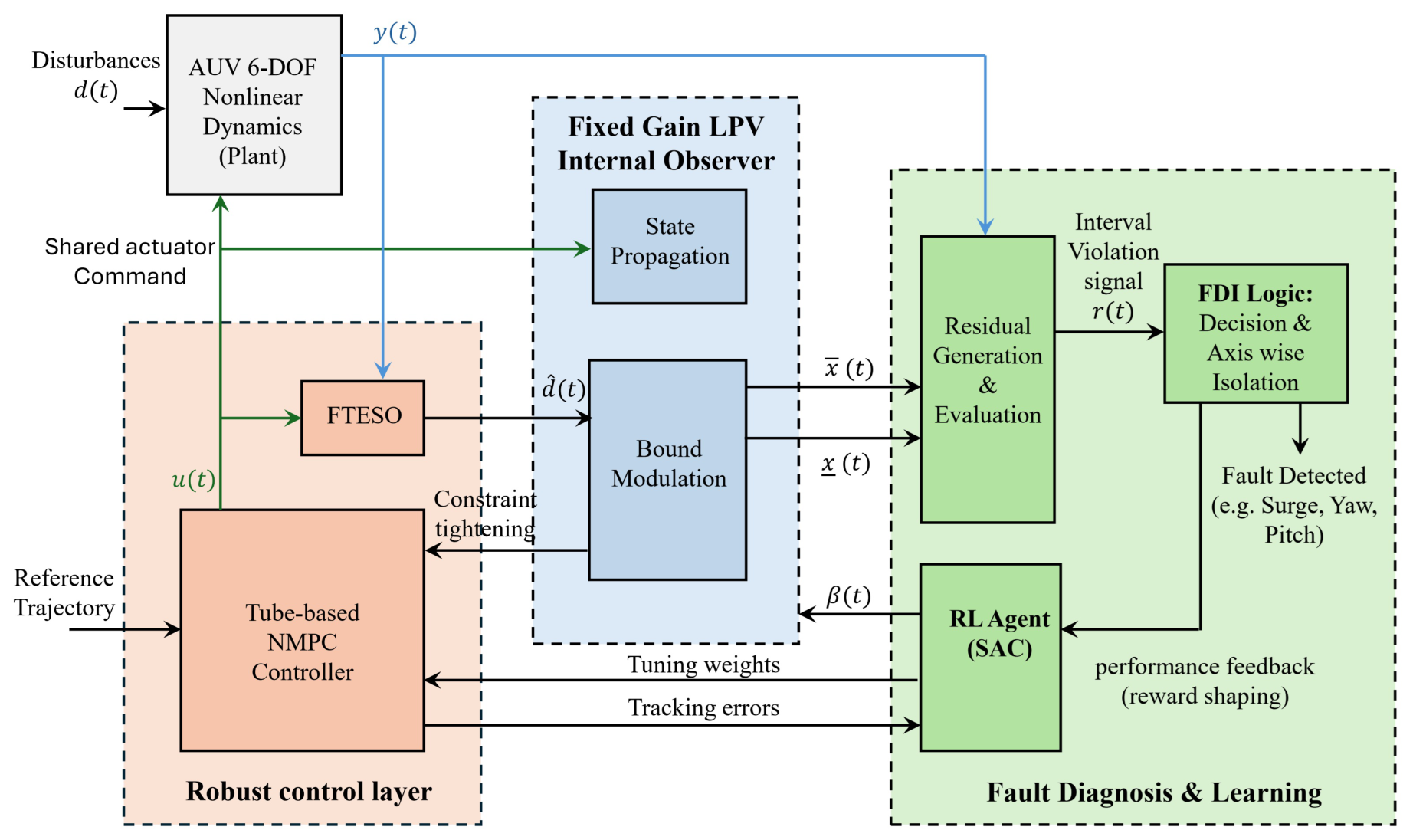
The proposed diagnosis architecture operates alongside the TNMPC/FTESO control loop, as illustrated in Figure 2. TNMPC generates a single actuator-command vector $\mathit{u}\left(t\right)$, whose branches supply the plant, FTESO, and nominal observer; they do not represent separate controller outputs. The FTESO supplies the bounded-error reconstructed measurement defined in (22) without altering the RAPIO state-propagation model.

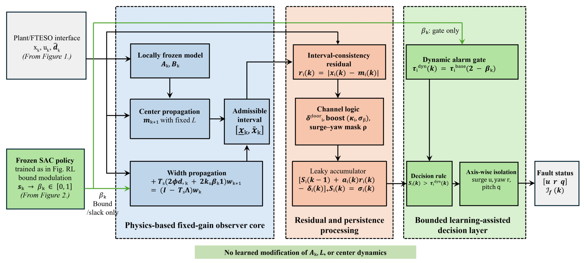
Using the locally frozen model of Section 2.2, RAPIO propagates an admissible tube for fault-free behavior. Persistent interval violations in ${\mathcal{I}}_d=\{u,r,q\}$ provide evidence of surge, rudder/yaw, and stern-plane/pitch faults, respectively. The learned scalar $\beta \left(t\right)$ adapts only the admissible uncertainty bound, while the observer matrices, scheduled gain, and decision structure remain model-based.

3.1. Interval Observer for Locally Frozen Dynamics

Recalling the nonlinear fault-affected AUV dynamics (13), the system is described by

$$\dot{\mathit{x}}\left(t\right)=f\left(\mathit{x}\left(t\right),\mathit{u}\left(t\right)\right)+\mathit{d}\left(t\right)+\mathit{F}{\mathit{f}}_a\left(t\right),$$

(24)

where $f\left(·\right)$ is locally Lipschitz in $\mathit{x}$, $\mathit{d}\left(t\right)$ denotes bounded disturbances, and ${\mathit{f}}_a\left(t\right)$ represents unknown actuator fault inputs.

Let $t_k$ denote a sampling instant and define the operating point $\left(\mathit{x}\left(t_k\right),\mathit{u}\left(t_k\right)\right)$. A first-order Taylor expansion of $f(\mathit{x},\mathit{u})$ about this point gives

$$\begin{array}{cc}\hfill f\left(\mathit{x}\right(t),\mathit{u}(t\left)\right)& =f\left(\mathit{x}\left(t_k\right),\mathit{u}\left(t_k\right)\right)+{\mathit{A}}_k\left(\mathit{x}\left(t\right)-\mathit{x}\left(t_k\right)\right)\hfill \\ \hfill & +{\mathit{B}}_k\left(\mathit{u}\left(t\right)-\mathit{u}\left(t_k\right)\right)+\mathbf{\Delta }\left(t\right),\hfill \end{array}$$

(25)

where

$${\mathit{A}}_k={\left.{\displaystyle \frac{\partial f}{\partial \mathit{x}}}\right|}_{(\mathit{x}\left(t_k\right),\mathit{u}\left(t_k\right))},{\mathit{B}}_k={\left.{\displaystyle \frac{\partial f}{\partial \mathit{u}}}\right|}_{(\mathit{x}\left(t_k\right),\mathit{u}\left(t_k\right))},$$

and $\mathbf{\Delta }\left(t\right)$ denotes the higher-order remainder. Since f is twice continuously differentiable over ${\mathcal{Z}}_c={\mathcal{X}}_c\times {\mathcal{U}}_c$, Taylor’s theorem ensures that there exists a scalar $L_{\Delta }>0$ such that the vector remainder $\mathbf{\Delta }\left(t\right)\in {\mathbb{R}}^{n_x}$ satisfies

$$\parallel \mathbf{\Delta }\left(t\right)\parallel \le L_{\Delta }{\parallel \mathit{z}\left(t\right)-\mathit{z}\left(t_k\right)\parallel }^2,t\in [t_k,t_{k+1}).$$

(26)

where $\mathit{z}\left(t\right)={[{\mathit{x}}^{\top }\left(t\right),{\mathit{u}}^{\top }\left(t\right)]}^{\top }$. Since $T_s$ satisfies (4), the trajectory remains inside ${\mathcal{Z}}_c$ and there exists $\overline{\Delta }>0$ such that

$$\parallel \mathbf{\Delta }\left(t\right)\parallel \le \overline{\Delta },\forall t\in [t_k,t_{k+1}),$$

(27)

with $\overline{\Delta }=L_{\Delta }{sup}_{t\in [t_k,t_{k+1})}{\parallel \mathit{z}\left(t\right)-\mathit{z}\left(t_k\right)\parallel }^2$.

The Jacobian ${\mathit{A}}_k$ is re-evaluated at every sampling instant $t_k$, so the observer tracks operating-point changes at the sampling rate. Criterion (4) keeps the within-sample linearization residual inside the admissible disturbance envelope. High-speed maneuvers or abrupt input changes can still be handled by faster refreezing or by enlarging the disturbance envelope, with the corresponding increase in interval width. Substituting (25) into (24) yields the locally frozen model

$$\dot{\mathit{x}}\left(t\right)={\mathit{A}}_k\mathit{x}\left(t\right)+{\mathit{B}}_k\mathit{u}\left(t\right)+\tilde{\mathit{d}}\left(t\right)+\mathit{F}{\mathit{f}}_a\left(t\right),$$

(28)

where the aggregated disturbance is defined in (29):

$$\tilde{\mathit{d}}\left(t\right):=\mathit{d}\left(t\right)+\mathbf{\Delta }\left(t\right)+{\mathit{\xi }}_k\left(t\right),$$

(29)

with ${\mathit{\xi }}_k\left(t\right)=f(\mathit{x}\left(t_k\right),\mathit{u}\left(t_k\right))-{\mathit{A}}_k\mathit{x}\left(t_k\right)-{\mathit{B}}_k\mathit{u}\left(t_k\right)$.

Under (27), the disturbance envelope ${\mathit{\varphi }}_d\left(t\right)\in {\mathbb{R}}_{\ge 0}^{n_x}$ is defined as a componentwise radius that upper-bounds the effective aggregate disturbance entering the interval-error dynamics, including physical disturbance, Taylor remainder, frozen-point offset, and bounded measurement/reconstruction error. It is selected before propagation so that

$${\mathit{\varphi }}_d\left(t\right)\ge \left|\mathit{d}\left(t\right)\right|+\overline{\Delta }{\mathbf{1}}_{n_x}+|{\mathit{\xi }}_k\left(t\right)|+|{\mathit{L}}_k|{\overline{\mathit{n}}}_y,\forall t,$$

(30)

where ${\mathbf{1}}_{n_x}$ is the $n_x$-dimensional all-ones vector, so the scalar Taylor bound $\overline{\Delta }$ is applied componentwise. Here ${\mathit{\varphi }}_d\left(t\right)$ is the componentwise disturbance envelope, $\overline{\Delta }$ bounds the Taylor remainder, ${\mathit{\xi }}_k\left(t\right)$ is the frozen linearization offset, ${\mathit{L}}_k$ is the observer gain introduced in (43), and ${\overline{\mathit{n}}}_y$ bounds measurement/reconstruction error with componentwise entries ${\overline{n}}_{y,i}={\overline{e}}_i$ from (22). Define the effective disturbance entering the observer error dynamics as

$${\tilde{\mathit{d}}}_o\left(t\right):=\tilde{\mathit{d}}\left(t\right)-{\mathit{L}}_k{\mathit{n}}_y\left(t\right).$$

(31)

where ${\tilde{\mathit{d}}}_o\left(t\right)$ is the disturbance seen by the observer error dynamics and ${\mathit{n}}_y\left(t\right)$ is the bounded measurement error. The triangle inequality then gives the componentwise bound in (32):

$$|{\tilde{\mathit{d}}}_o\left(t\right)|\le {\mathit{\varphi }}_d\left(t\right),\forall t.$$

(32)

The (33):

$${\mathit{\varphi }}_d\left(t\right)=\eta \left|{\widehat{\mathit{d}}}_o\left(t\right)\right|+\epsilon {\mathbf{1}}_{n_x},$$

(33)

where $\eta ={\Delta }_{max}$ is a fixed worst-case proportional uncertainty scaling factor and $\epsilon >0$ is a fixed additive robustness margin. The vector ${\widehat{\mathit{d}}}_o\left(t\right)\in {\mathbb{R}}^{n_x}$ is the FTESO-derived disturbance estimate lifted to the state-dynamics ordering; its first six entries are the generalized dynamic disturbance estimates and its kinematic entries are zero.

Remark 2.

The envelope parameters are fixed offline as $\eta ={\Delta }_{max}=0.5$ and $\epsilon =0.5$. Thus, η is not selected from the realized perturbation level of a scenario case. Online variation comes only through the FTESO estimate $|{\widehat{\mathit{d}}}_o\left(t\right)|$: larger estimated disturbances widen the tube, while calm conditions keep it tight. Channel-specific linearization-error allowances are included in the width update using $5\%$ of the estimated surge speed, $10\%$ of the estimated yaw rate plus a $0.08$ rad/s floor, and $5\%$ of the estimated heave velocity. Larger η and ε improve inclusion robustness but increase the minimum detectable fault magnitude in (60). These values are verified to satisfy (30) over the maneuvering envelope ${\mathcal{Z}}_c$ by offline calibration: the additive floor $\epsilon =0.5$ absorbs the worst-case sum $|\mathbf{\Delta }|+|{\mathit{\xi }}_k|+|{\mathit{L}}_k|{\overline{\mathit{n}}}_y$ computed from nominal and perturbed simulation cases, while the proportional term $\eta |{\widehat{\mathit{d}}}_o|$ tracks the time-varying physical disturbance. Any operating regime with larger $\parallel \mathbf{\Delta }\parallel$ (e.g., high-speed maneuvers exceeding the calibration envelope) would require a larger ε or a reduced $T_s$ per (4).

Table 1. Qualitative effect of varying the disturbance-envelope parameters $\eta$ and $\epsilon$ from the nominal design. Detectability margin references (60); false-alarm risk is assessed relative to the nominal zero-false-alarm benchmark result.

$\mathit{\eta }$	$\mathit{\epsilon }$	Inclusion Margin	Detectability Effect	False-Alarm Risk
0.25	0.25	Reduced; tighter tube	Lower minimum detectable fault; improved sensitivity	Increased if true disturbance exceeds the tighter envelope
0.50	0.50	Nominal (scenario-sweep verified)	Minimum detectable: 0.18 m/s, 0.09 rad/s, 0.42 m/s	Zero across all 72 scenario cases
0.75	0.75	Enlarged; wider tube	Higher minimum detectable fault; reduced sensitivity	Near zero; wider tube keeps healthy residuals well within bounds, but the same envelope also absorbs small fault signatures (see Detectability effect)

summarizes the qualitative effect of varying both parameters from the nominal design.

The admissible state set in (34) is represented by the two boundary observers ${\mathit{x}}^{-}\left(t\right)$ and ${\mathit{x}}^{+}\left(t\right)$:

$$\mathcal{X}\left(t\right)=\left\{\mathit{x}\in {\mathbb{R}}^{n_x}|{\mathit{x}}^{-}\left(t\right)\le \mathit{x}\le {\mathit{x}}^{+}\left(t\right)\right\}.$$

(34)

Let

$${\mathit{A}}_{o,k}:={\mathit{A}}_k-{\mathit{L}}_k\mathit{C}$$

denote the frozen observer error matrix. The observer gain ${\mathit{L}}_k$ is selected by a deterministic scheduling rule so that ${\mathit{A}}_{o,k}$ is Metzler and Hurwitz at each sampled operating point.

The two boundary observers are

$${\dot{\mathit{x}}}^{+}\left(t\right)={\mathit{A}}_{o,k}{\mathit{x}}^{+}\left(t\right)+{\mathit{B}}_k\mathit{u}\left(t\right)+{\mathit{L}}_k\mathit{y}\left(t\right)+{\mathit{\varphi }}_d\left(t\right)+\mathbf{\Gamma }\left(t\right),$$

(35)

$${\dot{\mathit{x}}}^{-}\left(t\right)={\mathit{A}}_{o,k}{\mathit{x}}^{-}\left(t\right)+{\mathit{B}}_k\mathit{u}\left(t\right)+{\mathit{L}}_k\mathit{y}\left(t\right)-{\mathit{\varphi }}_d\left(t\right)-\mathbf{\Gamma }\left(t\right),$$

(36)

where $\mathit{C}={\mathit{I}}_{n_x}={\mathit{I}}_{12}$, $\mathit{y}$ is the reconstructed full-state output defined in (22), and $\mathbf{\Gamma }\left(t\right)\in {\mathbb{R}}_{\ge 0}^{n_x}$ is a nonnegative width-slack input, parameterized explicitly in (55). The full-state output $\mathit{C}={\mathit{I}}_{12}$ is an idealization of direct state access; Proposition 2 shows the inclusion results extend to any bounded-error state reconstructor, covering practical FTESO-based AUV implementations. Equivalently, the observer can be written in center and half-width variables

$$\mathit{m}\left(t\right)=\frac{1}{2}\left({\mathit{x}}^{+}\left(t\right)+{\mathit{x}}^{-}\left(t\right)\right),\mathbf{\delta }\left(t\right)=\frac{1}{2}\left({\mathit{x}}^{+}\left(t\right)-{\mathit{x}}^{-}\left(t\right)\right),$$

(37)

which gives the same plotted tube $\left[\mathit{m}\right(t)-\mathbf{\delta }(t),\mathit{m}(t)+\mathbf{\delta }(t\left)\right]$. The center estimate follows a prediction-correction scheme with a separate small scalar gain $\gamma \in (0,1)$:

$${\mathit{m}}_{k+1}^p=f_{\mathrm{nom}}\left({\mathit{m}}_k^c,{\mathit{u}}_k\right),$$

(38)

$${\mathit{m}}_{k+1}^c={\mathit{m}}_{k+1}^p+\gamma {\mathit{H}}_{k+1}\left({\mathit{y}}_{k+1}-{\mathit{m}}_{k+1}^p\right),$$

(39)

where $f_{\mathrm{nom}}\left(·\right)$ denotes the nominal plant predictor with $\mathit{\alpha }=\mathbf{1}$ and the recorded actuator commands. The diagonal matrix ${\mathit{H}}_{k+1}=diag(h_{1,k+1},\dots ,h_{n_x,k+1})$ is the detector-gated correction mask. For non-diagnostic states $h_{i,k+1}=1$. For diagnostic axes $i\in {\mathcal{I}}_d$, $h_{i,k+1}=0$ while the corresponding channel is in the confirmed-alarm freeze state, and $h_{i,k+1}=1$ otherwise. Detection uses ${\mathit{m}}_{k+1}^p$ (before correction); the gated correction ${\mathit{m}}_{k+1}^c$ prepares the center for the subsequent prediction step. Thus, when a channel is alarmed, only its measurement-correction term is suspended. The center continues to evolve through the nominal predictor (38).

Remark 3.

The center gain γ and the width gain ${\mathit{L}}_k$ serve distinct roles and are chosen independently. ${\mathit{L}}_k$ is a large Metzler-scheduled gain that ensures ${\mathit{A}}_{o,k}={\mathit{A}}_k-{\mathit{L}}_k\mathit{C}$ is Metzler and Hurwitz (providing the formal width-bounding certificate). γ is a small scalar ($\gamma \ll {\ell }_i{T}_s$) chosen so that the center tracks the nominal trajectory without being pulled toward fault-affected measurements. The gate ${\mathit{H}}_{k+1}$ further prevents a confirmed faulty diagnostic channel from dragging its own center toward the fault response. Using ${\mathit{L}}_k$ for the center would cause the center estimate to follow fault-induced measurement excursions, eliminating the fault residual and defeating detection.

The interval certificate is associated with the two boundary observers (35) and (36). In the discrete implementation, the center follows (38) and (39) rather than a continuous Luenberger form; the center-width decomposition $\mathit{m}=\frac{1}{2}({\mathit{x}}^{+}+{\mathit{x}}^{-})$, $\mathbf{\delta }=\frac{1}{2}({\mathit{x}}^{+}-{\mathit{x}}^{-})$ defined in (37) remains valid at each step. A sufficient initialization condition for guaranteed enclosure is ${\mathit{x}}^{-}\left(0\right)\le \mathit{x}\left(0\right)\le {\mathit{x}}^{+}\left(0\right)$; in the simulations ${\mathit{m}}_0^c=\mathit{x}\left(0\right)$ and $\mathbf{\delta }\left(0\right)\ge \mathbf{0}$ make this condition trivially satisfied. The formal componentwise enclosure in (40)

$${\mathit{x}}^{-}\left(t\right)\le \mathit{x}\left(t\right)\le {\mathit{x}}^{+}\left(t\right),\forall t\ge 0,$$

(40)

is established directly from positivity of Metzler systems in Section 3.2.

Subtracting (36) from (35) gives the boundary separation $\mathit{w}\left(t\right)={\mathit{x}}^{+}\left(t\right)-{\mathit{x}}^{-}\left(t\right)=2\mathbf{\delta }\left(t\right)$:

$$\dot{\mathit{w}}\left(t\right)={\mathit{A}}_{o,k}\mathit{w}\left(t\right)+2{\mathit{\varphi }}_d\left(t\right)+2\mathbf{\Gamma }\left(t\right).$$

(41)

where $\mathit{w}\left(t\right)$ is the interval width, ${\mathit{A}}_{o,k}$ is the observer error matrix, ${\mathit{\varphi }}_d\left(t\right)$ is the disturbance envelope, and $\mathbf{\Gamma }\left(t\right)$ is the additional slack input. Dividing by two and writing $\mathbf{\delta }\left(t\right)=\frac{1}{2}\mathit{w}\left(t\right)$ gives the half-width dynamics

$$\dot{\mathbf{\delta }}\left(t\right)={\mathit{A}}_{o,k}\mathbf{\delta }\left(t\right)+{\mathit{\varphi }}_d\left(t\right)+\mathbf{\Gamma }\left(t\right),$$

(42)

which is the form integrated by the Van Loan augmented matrix exponential in Remark 4. Actuator faults ${\mathit{f}}_a\left(t\right)$ do not enter (41). Disturbances are absorbed by the boundary separation, whereas persistent actuator faults induce exits from the interval $[{\mathit{x}}^{-}\left(t\right),{\mathit{x}}^{+}\left(t\right)]$, enabling detection.

3.2. Stability and Interval Inclusion Guarantees

This subsection establishes boundedness, stability, and guaranteed interval inclusion for the tube-based observer of Section 3.1. All results are derived for the fault-free case ${\mathit{f}}_a\left(t\right)\equiv \mathbf{0}$.

Assumption 4

([10,15]). For each frozen operating point $\mathit{\rho }\left(t_k\right)$, the observer gain ${\mathit{L}}_k\in {\mathbb{R}}^{n_x\times n_x}$ is constructed by the deterministic scheduling rule

$${\left[{\mathit{L}}_k\right]}_{ii}={\ell }_i,{\left[{\mathit{L}}_k\right]}_{ij}=min\left(0,{\left[{\mathit{A}}_k\right]}_{ij}-{\mu }_c\right),i\ne j,$$

(43)

where ${\ell }_i>0$ are fixed diagonal seeds and ${\mu }_c>0$ is a cooperative margin, both selected as fixed observer-design parameters. The symbol ${\mu }_c$ is used to distinguish this observer-design margin from the vehicle mass m. For every off-diagonal pair $(i,j)$, the closed-loop matrix ${\mathit{A}}_{o,k}:={\mathit{A}}_k-{\mathit{L}}_k\mathit{C}$ then satisfies the Metzler condition in (44):

$${\left[{\mathit{A}}_{o,k}\right]}_{ij}={\left[{\mathit{A}}_k\right]}_{ij}-min\left(0,{\left[{\mathit{A}}_k\right]}_{ij}-{\mu }_c\right)=max\left({\left[{\mathit{A}}_k\right]}_{ij},{\mu }_c\right)\ge {\mu }_c>0,$$

(44)

where ${\left[{\mathit{A}}_{o,k}\right]}_{ij}$ is an off-diagonal entry of the closed-loop observer matrix and ${\mu }_c$ is the cooperative margin. The inequality holds regardless of the sign of ${\left[{\mathit{A}}_k\right]}_{ij}$, including all Coriolis and hydrodynamic coupling terms. ${\mathit{A}}_{o,k}$ is therefore Metzler by construction at every operating point. This gain design is always feasible: for any frozen ${\mathit{A}}_k$, choosing ${\ell }_i$ to exceed the largest row-sum of positive off-diagonal entries of ${\mathit{A}}_k$ plus a margin is sufficient to make ${\mathit{A}}_{o,k}$ both Metzler and Hurwitz simultaneously. The diagonal seeds ${\ell }_i$ are selected offline to provide contraction on the tested operating envelope and are verified by the certificate below. At each update, the triple certificate

$$\underset{i\ne j}{min}{\left[{\mathit{A}}_{o,k}\right]}_{ij}\ge 0,\underset{i}{max}Re\left({\lambda }_i\left({\mathit{A}}_{o,k}\right)\right)\le -{\lambda }_{★}<0,\underset{i,j}{min}{\left[e^{{\mathit{A}}_{o,k}{T}_s}\right]}_{ij}\ge 0$$

(45)

is imposed on the sampled operating envelope, where ${\lambda }_{★}>0$ is the certified uniform decay margin, ${\lambda }_i\left({\mathit{A}}_{o,k}\right)$ denotes the i-th eigenvalue, $Re\left(·\right)$ its real part, and $T_s$ the diagnostic update period. The off-diagonal entries of ${\mathit{L}}_k$ are mathematical observer-gain entries used to enforce cooperativity; they are not restricted to be sensor weights. The certificate is verified numerically over the same diagnostic update interval used in the Van Loan width propagation and logged at run time.

Remark 4.

The AUV Jacobian ${\mathit{A}}_k$ carries Coriolis and hydrodynamic coupling terms whose signs change with surge speed, yaw rate and depth. It reflects the underactuated, coupled nature of the vehicle. The scheduling rule (43) handles this by construction. Every off-diagonal entry of ${\mathit{A}}_{o,k}$ is brought to at least ${\mu }_c>0$ regardless of the sign of ${\left[{\mathit{A}}_k\right]}_{ij}$. The half-width ODE (42) is then discretized exactly over $[t_k,t_{k+1})$ via the Van Loan augmented matrix exponential, yielding the update ${\mathbf{\Phi }}_k{\mathbf{\delta }}_k+{\mathit{\psi }}_k$ with ${\mathbf{\Phi }}_k,{\mathit{\psi }}_k\ge \mathbf{0}$. The implementation applies the Müller form $|{\mathbf{\Phi }}_k|{\mathbf{\delta }}_k+\left|{\mathit{\psi }}_k\right|$ as a floating-point safeguard against Jacobian rounding near the cooperative margin and the triple certificate (45) is logged at every update step.

Assumption 5

([10,12]). This condition is a consequence of Assumptions 1–3 and the envelope construction (30); it is stated separately for clarity in the stability proof. The effective disturbance entering the observer error dynamics satisfies (46):

$$|{\tilde{\mathit{d}}}_o\left(t\right)|\le {\mathit{\varphi }}_d\left(t\right),$$

(46)

where ${\mathit{\varphi }}_d\left(t\right)\in {\mathbb{R}}^{n_x}$ is componentwise nonnegative, uniformly bounded, and piecewise continuous.

Assumption 6

([10,12,37]). As a design choice that preserves the nonnegative bounded-input structure of the width dynamics, the slack term is parameterized as $\mathbf{\Gamma }\left(t\right)=\left(1-\beta \left(t\right)\right){\mathit{d}}^{\mathrm{slack}}$, ${\mathit{d}}^{\mathrm{slack}}\ge \mathbf{0}$, $\beta \left(t\right)\in [0,1]$, giving the interval width dynamics

$$\dot{\mathit{w}}\left(t\right)={\mathit{A}}_{o,k}\mathit{w}\left(t\right)+2{\mathit{\varphi }}_d\left(t\right)+2\left(1-\beta \left(t\right)\right){\mathit{d}}^{\mathrm{slack}}.$$

(47)

where $\mathit{w}\left(t\right)$ is the interval width and ${\mathit{d}}^{\mathrm{slack}}$ is the nonnegative maximum slack vector. Because ${\mathit{A}}_{o,k}$ is Metzler and Hurwitz, these dynamics form a positive and stable comparison system. The learning signal enters only through the nonnegative bounded input $\left(1-\beta \left(t\right)\right){\mathit{d}}^{\mathrm{slack}}$.

Lemma 1.

Given $\mathit{w}\left(0\right)\ge \mathbf{0}$, the width $\mathit{w}\left(t\right)$ defined by (47) remains componentwise nonnegative and uniformly ultimately bounded for all $t\ge 0$.

Proof. 

Since ${\mathit{A}}_{o,k}$ is Metzler, $e^{{\mathit{A}}_{o,k}t}$ is componentwise nonnegative for all $t\ge 0$. With $\mathit{b}\left(t\right)=2{\mathit{\varphi }}_d\left(t\right)+2(1-\beta \left(t\right)){\mathit{d}}^{\mathrm{slack}}\ge \mathbf{0}$, the variation-of-constants formula gives (48):

$$\mathit{w}\left(t\right)=e^{{\mathit{A}}_{o,k}t}\mathit{w}\left(0\right)+{\int }_0^t{e}^{{\mathit{A}}_{o,k}(t-\tau )}\mathit{b}\left(\tau \right)d\tau .$$

(48)

This proves nonnegativity on $[t_k,t_{k+1})$. Since ${\mathit{A}}_{o,k}$ updates at each $t_k$, the argument applies piecewise. At each $t_k$, continuity of ${\mathit{x}}^{+}$ and ${\mathit{x}}^{-}$ gives $\mathit{w}\left(t_k\right)\ge \mathbf{0}$ as the initial condition for the next frozen interval, therefore proving propagating nonnegativity by induction. Boundedness follows from the uniform certificate in (45). Since ${max}_{i}Re\left({\lambda }_i\left({\mathit{A}}_{o,k}\right)\right)\le -{\lambda }_{★}<0$ for all sampled frozen matrices and $\mathit{b}\left(t\right)$ is uniformly bounded, the positive switched comparison system admits a common finite envelope. Equivalently, for each frozen interval the componentwise steady bound $-{\mathit{A}}_{o,k}^{-1}\overline{\mathit{b}}$ is finite, and the uniform decay margin prevents growth under the scheduled updates. Here $\overline{\mathit{b}}:={sup}_{t\ge 0}\mathit{b}\left(t\right)$ denotes any finite componentwise upper bound on the nonnegative input $\mathit{b}\left(t\right)=2{\mathit{\varphi }}_d\left(t\right)+2\mathbf{\Gamma }\left(t\right)$.    □

Proposition 1.

Let $D_i>0$ denote the componentwise one-step prediction-error bound calibrated from nominal operation on the diagnostic axes ${\mathcal{I}}_d$:

$$\left|{\tilde{e}}_{m,i}\left(k\right)\right|:=\left|x_i\left(k\right)-m_i^p\left(k\right)\right|\le D_i,i\in {\mathcal{I}}_d,$$

(49)

where ${\tilde{e}}_{m,i}$ is the center prediction error before correction. Let ${\mathbf{\Phi }}_k=e^{{\mathit{A}}_{o,k}{T}_s}$ and let ${\mathit{\psi }}_k$ denote the Van Loan input generated using $d_{\mathrm{rate},i}=D_i/T_s$. If the calibrated input satisfies

$$|{\tilde{\mathit{e}}}_m(k+1)|\le {\mathbf{\Phi }}_k\left|{\tilde{\mathit{e}}}_m\left(k\right)\right|+{\mathit{\psi }}_k,$$

(50)

then ${\delta }_i\left(0\right)\ge D_i$ implies ${\delta }_i\left(k\right)\ge \left|{\tilde{e}}_{m,i}\left(k\right)\right|$ for all $k\ge 0$, and hence, $x_i^{-}\left(k\right)\le x_i\left(k\right)\le x_i^{+}\left(k\right)$ on ${\mathcal{I}}_d$.

Proof. 

Metzlerness gives ${\mathbf{\Phi }}_k\ge \mathbf{0}$ and, since ${\mathit{d}}_{\mathrm{rate}}\ge \mathbf{0}$, also ${\mathit{\psi }}_k\ge \mathbf{0}$. Combining the width recursion with (50) yields

$$\mathbf{\delta }(k+1)-|{\tilde{\mathit{e}}}_m(k+1)|\ge {\mathbf{\Phi }}_k\left(\mathbf{\delta }\left(k\right)-|{\tilde{\mathit{e}}}_m\left(k\right)|\right)\ge \mathbf{0}.$$

(51)

Because $\mathbf{\delta }\left(0\right)\ge \mathit{D}\ge |{\tilde{\mathit{e}}}_m\left(0\right)|$, induction gives $\mathbf{\delta }\left(k\right)\ge |{\tilde{\mathit{e}}}_m\left(k\right)|$ for every k, which is equivalent to the stated interval framing.    □

Theorem 1.

Suppose Assumptions 4–6 hold and ${\mathit{x}}^{-}\left(0\right)\le \mathit{x}\left(0\right)\le {\mathit{x}}^{+}\left(0\right)$. Then, in the absence of actuator faults,

$${\mathit{x}}^{-}\left(t\right)\le \mathit{x}\left(t\right)\le {\mathit{x}}^{+}\left(t\right),\forall t\ge 0.$$

(52)

where ${\mathit{x}}^{-}\left(t\right)$ and ${\mathit{x}}^{+}\left(t\right)$ are the lower and upper interval bounds and $\mathit{x}\left(t\right)$ is the true plant state.

Proof. 

Define the upper and lower enclosure errors ${\mathit{e}}^{+}\left(t\right)={\mathit{x}}^{+}\left(t\right)-\mathit{x}\left(t\right)$ and ${\mathit{e}}^{-}\left(t\right)=\mathit{x}\left(t\right)-{\mathit{x}}^{-}\left(t\right)$. Subtracting the plant (28) from the upper observer (35) and using $\mathit{y}=\mathit{x}+{\mathit{n}}_y$ together with definition (31) gives ${\mathit{L}}_k\mathit{y}+\tilde{\mathit{d}}\left(t\right)={\mathit{L}}_k\mathit{x}+{\tilde{\mathit{d}}}_o\left(t\right)$, yielding

$${\dot{\mathit{e}}}^{+}\left(t\right)={\mathit{A}}_{o,k}{\mathit{e}}^{+}\left(t\right)+{\mathit{\varphi }}_d\left(t\right)+\mathbf{\Gamma }\left(t\right)-{\tilde{\mathit{d}}}_o\left(t\right),$$

(53)

$${\dot{\mathit{e}}}^{-}\left(t\right)={\mathit{A}}_{o,k}{\mathit{e}}^{-}\left(t\right)+{\mathit{\varphi }}_d\left(t\right)+\mathbf{\Gamma }\left(t\right)+{\tilde{\mathit{d}}}_o\left(t\right).$$

(54)

The enclosure-error dynamics in (53) and (54) are positive comparison systems. By Assumption 5, ${\mathit{\varphi }}_d\left(t\right)\pm {\tilde{\mathit{d}}}_o\left(t\right)\ge \mathbf{0}$, and $\mathbf{\Gamma }\left(t\right)\ge \mathbf{0}$. Since ${\mathit{A}}_{o,k}$ is Metzler, the comparison systems for ${\mathit{e}}^{+}$ and ${\mathit{e}}^{-}$ are positive. The initialization ${\mathit{x}}^{-}\left(0\right)\le \mathit{x}\left(0\right)\le {\mathit{x}}^{+}\left(0\right)$ gives ${\mathit{e}}^{+}\left(0\right)\ge \mathbf{0}$ and ${\mathit{e}}^{-}\left(0\right)\ge \mathbf{0}$, hence ${\mathit{e}}^{+}\left(t\right),{\mathit{e}}^{-}\left(t\right)\ge \mathbf{0}$ for all $t\ge 0$. Therefore, ${\mathit{x}}^{-}\left(t\right)\le \mathit{x}\left(t\right)\le {\mathit{x}}^{+}\left(t\right)$ componentwise, which proves (52).    □

3.3. RL-Augmented Uncertainty Bound Modulation

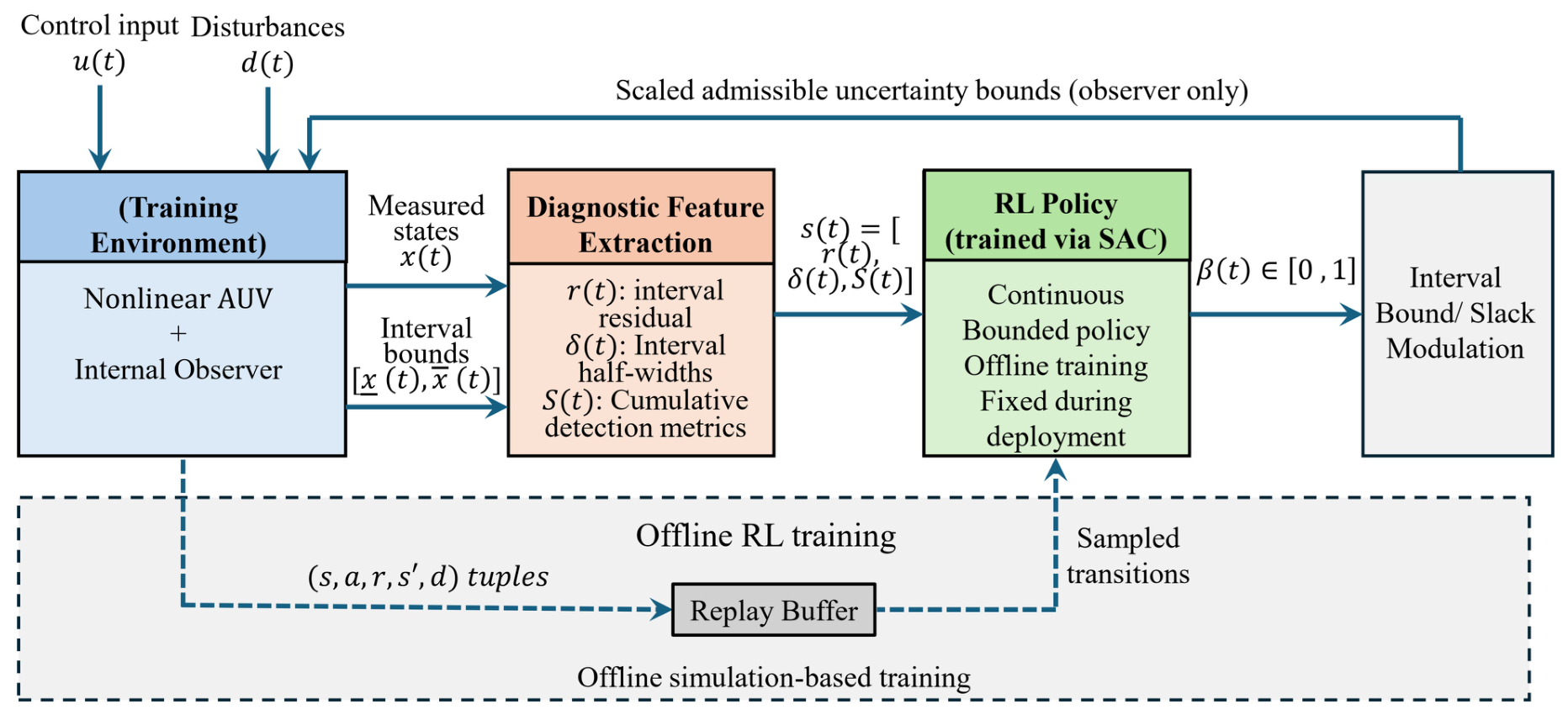
RL-augmented uncertainty bound modulation is introduced as a bounded exogenous input acting exclusively on the interval width dynamics, with the objective of enhancing disturbance accommodation while preserving the guarantees of Section 3.2. As illustrated in Figure 3, the learning module is structurally decoupled from the center estimation dynamics and the plant model.

The learning signal enters the width dynamics exclusively through a bounded confidence-dependent slack: high confidence tightens the disturbance-rate slack and low confidence widens it:

$$\mathbf{\Gamma }\left(t\right)=\left(1-\beta \left(t\right)\right){\mathit{d}}^{\mathrm{slack}},\beta \left(t\right)\in [0,1],{\mathit{d}}^{\mathrm{slack}}\ge \mathbf{0},$$

(55)

where $\mathbf{\Gamma }\left(t\right)$ is the learning-modulated slack input, $\beta \left(t\right)$ is the bounded RL confidence signal, and ${\mathit{d}}^{\mathrm{slack}}$ is the maximum channel-wise slack. The corresponding learning-modulated width dynamics are given by Equation (47), where $\mathit{w}\left(t\right)$ is the interval width and ${\mathit{A}}_{o,k}$, ${\mathit{\varphi }}_d\left(t\right)$, $\beta \left(t\right)$, and ${\mathit{d}}^{\mathrm{slack}}$ retain the definitions given above.

By Lemma 1, $\mathit{w}\left(t\right)$ remains nonnegative and uniformly bounded. Learning therefore enlarges the admissible tube only through the bounded input $2(1-\beta \left(t\right)){\mathit{d}}^{\mathrm{slack}}$ and does not modify ${\mathit{A}}_{o,k}$ or its Metzler/Hurwitz certificate.

The center prediction-error bound (49) is independent of $\beta \left(t\right)$ because $\beta$ modulates only the disturbance-rate slack fed into the Van Loan width update. Consequently, the framing guarantee of Proposition 1 holds for all admissible $\beta \left(t\right)$.

Let ${\mathit{e}}_m\left(t\right):=\mathit{x}\left(t\right)-\mathit{m}\left(t\right)$ denote the interval-center error and let the superscript $\mathrm{ss}$ denote its persistent steady value. For a single actuator fault ${\mathit{f}}_a\left(t\right)={\overline{f}}_j{\mathit{e}}_j$, decompose the steady-state center error as

$${\mathit{e}}_m^{\mathrm{ss}}=-{\mathit{A}}_{o,k}^{-1}\left({\tilde{\mathit{d}}}^{\mathrm{ss}}+\mathit{F}{\overline{f}}_j{\mathit{e}}_j\right).$$

(56)

where ${\mathit{e}}_m^{\mathrm{ss}}$ is the steady-state center error, ${\tilde{\mathit{d}}}^{\mathrm{ss}}$ is the steady-state aggregate disturbance, ${\overline{f}}_j$ is the persistent fault magnitude in actuator channel j, and ${\mathit{e}}_j$ is the corresponding canonical basis vector in ${\mathbb{R}}^3$. Define the scalar fault-to-channel gain

$$g_{ij}:=\left|{\left[{\mathit{A}}_{o,k}^{-1}\mathit{F}\right]}_{ij}\right|,$$

(57)

where $g_{ij}$ is the scalar gain from actuator fault j to state channel i. Thus, $|{\left[{\mathit{A}}_{o,k}^{-1}\mathit{F}{\overline{f}}_j{\mathit{e}}_j\right]}_i|=g_{ij}\left|{\overline{f}}_j\right|$. Setting ${\kappa }_i={\parallel {\left[{\mathit{A}}_{o,k}^{-1}\right]}_{i,:}\parallel }_1$ and ${\eta }_i={\kappa }_i{sup}_t{\parallel \tilde{\mathit{d}}\left(t\right)\parallel }_{\infty }$, the reverse triangle inequality gives

$$|e_{m,i}^{\mathrm{ss}}|\ge g_{ij}\left|{\overline{f}}_j\right|-{\eta }_i,$$

(58)

where ${\eta }_i$ is a disturbance-induced bias bound and is distinct from the pose vector $\mathit{\eta }$ and the scalar envelope factor used elsewhere. In (60), ${\tau }_i^{\mathrm{base}}>0$ is the fixed accumulator threshold and ${\delta }_i^{\mathrm{floor}}>0$ is the residual noise floor; both are defined operationally in Section 3.4. Here $g_{ij}$ is a nonnegative scalar (the absolute value of a single matrix entry), so its use as the lower-bound coefficient in (58) is justified directly by the reverse triangle inequality without invoking any row-norm argument. Define the certified worst-case steady half-width by (59):

$${\overline{\delta }}_i:={\displaystyle \frac{1}{2}}\underset{k}{sup}{\left[-{\mathit{A}}_{o,k}^{-1}\left(2{\overline{\mathit{\varphi }}}_d+2{\mathit{d}}^{\mathrm{slack}}\right)\right]}_i,$$

(59)

where ${\overline{\delta }}_i$ is the certified worst-case steady half-width for channel i, ${\overline{\mathit{\varphi }}}_d$ is a componentwise upper bound on ${\mathit{\varphi }}_d\left(t\right)$ over the operating envelope, and the supremum is evaluated over the certified frozen matrices. This bound uses the coupled positive system directly rather than a scalar approximation. A sufficient offline detectability condition is

$$g_{ij}\left|{\overline{f}}_j\right|>{\overline{\delta }}_i+{\eta }_i+{\displaystyle \frac{1-{\sigma }_i}{{\sigma }_i}}{\tau }_i^{\mathrm{base}}+{\delta }_i^{\mathrm{floor}},$$

(60)

where ${\sigma }_i$ is the channel-specific leak of the accumulator in Section 3.4. The factor $(1-{\sigma }_i)/{\sigma }_i$ converts the fixed accumulated gate ${\tau }_i^{\mathrm{base}}$ into the required persistent residual excess, consistent with Proposition 3 and Remark 7.

Remark 5.

Condition (60) is a conservative offline separation check, not an online decision rule. The conservatism comes from using worst-case tube width, disturbance masking and frozen-Jacobian fault-to-channel gains. These quantities are used only during calibration. Online detection uses the propagated interval tube, directed cross-channel margins, and the fixed leaky accumulator of Section 3.4.

Theorem 2.

Suppose Assumptions 4–6 hold and ${\mathit{x}}^{-}\left(0\right)\le \mathit{x}\left(0\right)\le {\mathit{x}}^{+}\left(0\right)$. For any bounded measurable $\beta \left(t\right)\in [0,1]$, the RL-augmented interval observer preserves the componentwise inclusion condition (61) for every certified component i:

$$x_i^{-}\left(t\right)\le x_i\left(t\right)\le x_i^{+}\left(t\right),\forall t\ge 0,$$

(61)

where $x_i^{-}\left(t\right)$ and $x_i^{+}\left(t\right)$ are the lower and upper bounds of component i, and $x_i\left(t\right)$ is the corresponding true state component, in the absence of actuator faults.

Proof. 

$\beta \left(t\right)$ enters only the width subsystem (47) via the slack $(1-\beta ){\mathit{d}}^{\mathrm{slack}}$. It does not appear in the center prediction step (38) or in the detector mask ${\mathit{H}}_{k+1}$ of the correction step (39), and does not modify ${\mathit{A}}_{o,k}$, ${\mathit{L}}_k$, or the scheduled-gain rule (43). The Metzler/Hurwitz certificate therefore holds for all $\beta \left(t\right)\in [0,1]$, and the inclusion result of Theorem 1 applies without modification.    □

Proposition 2.

Suppose any stabilizing feedback law $\mathit{u}\left(t\right)=\pi \left(\mathit{x}\right(t\left)\right)$ keeps $\mathit{x}\left(t\right)\in {\mathcal{X}}_c$ for all $t\ge 0$, and any state reconstructor supplies $\widehat{\mathit{x}}\left(t_k\right)$ with the componentwise error bound in (62):

$$|x_i\left(t_k\right)-{\widehat{x}}_i\left(t_k\right)|\le {\overline{e}}_i,\forall t_k,\forall i.$$

(62)

Then Theorems 1 and 2 hold with the noise floor updated to ${\delta }_i^{\mathrm{floor}}={\overline{e}}_i+{\epsilon }_{\mathrm{buf}}$, independently of the specific form of $\pi \left(·\right)$ or the state reconstructor, provided the innovation-noise term is covered by $|{\mathit{L}}_k|{\overline{\mathit{n}}}_y$ in (30). In addition, zero healthy-operation accumulator growth requires the boundary-excess buffer ${\epsilon }_{\mathrm{buf},i}>0$ to dominate the reconstruction error margin.

Proof. 

The center prediction error at step k is ${\tilde{\mathit{e}}}_m\left(k\right)=\mathit{x}\left(k\right)-{\mathit{m}}^p\left(k\right)$, where ${\mathit{m}}^p\left(k\right)$ follows the prediction step (38). The nominal predictor uses the recorded command ${\mathit{u}}_{k-1}$, which is the same command applied to the plant (28); the control input therefore cancels in the prediction error regardless of the form of $\pi \left(·\right)$. The scheduled gain ${\mathit{L}}_k$ and frozen Jacobian ${\mathit{A}}_k$ do not depend on the controller structure. Measurement or reconstruction noise ${\mathit{n}}_y$ enters only through the correction step (39) with gain $\gamma {\mathit{H}}_{k+1}$; since $0\le h_{i,k+1}\le 1$, its contribution is bounded by $\gamma {\overline{\mathit{n}}}_y$ and is absorbed into ${\delta }_i^{\mathrm{floor}}$. Condition (30) covers the remaining disturbance terms entering the boundary observers, so Assumption 5 remains satisfied.

Since $\mathit{x}\left(t\right)\in {\mathcal{X}}_c$ is guaranteed by assumption, the Taylor remainder bound (26) and the slowly varying scheduling condition (2) hold, so Theorem 1 applies without modification to yield $x_i^{-}\left(t\right)\le x_i\left(t\right)\le x_i^{+}\left(t\right)$ for all i.

When $\widehat{\mathit{x}}\left(t_k\right)$ is used in the residual computation, the apparent boundary-excess residual satisfies ${\varrho }_i\left(k\right)\le {\overline{e}}_i$ in the fault-free case. If ${\epsilon }_{\mathrm{buf},i}>0$, then

$${\varrho }_i\left(k\right)\le {\overline{e}}_i<{\overline{e}}_i+{\epsilon }_{\mathrm{buf},i}={\delta }_i^{\mathrm{floor}},$$

and the accumulator does not grow in the fault-free case. Without this buffer, the bounded reconstruction error is still included in the residual bound, but zero accumulator growth is not guaranteed. The width dynamics (47) and the RL signal ${\beta }_k$ are unaffected by the controller or state reconstructor choice, completing the proof.    □

The learned signal ${\beta }_k$ does not change the observer gain, frozen Jacobian, nominal center predictor, detector gate, or alarm thresholds. It only modulates the sampled disturbance-rate slack used in the width propagation,

$$d_i\left(k\right)={\displaystyle \frac{D_i+(1-{\beta }_k)D_i^{\mathrm{slack}}}{T_s}},i\in {\mathcal{I}}_d,$$

where $d_i\left(k\right)$ is the sampled disturbance rate used in the width update, $D_i$ is the calibrated one-step disturbance bound, and $D_i^{\mathrm{slack}}$ is the maximum one-step RL-modulated slack. Its continuous-time counterpart in (55) is $d_i^{\mathrm{slack}}=D_i^{\mathrm{slack}}/T_s$. The quantities ${\beta }_k$, $T_s$, and ${\mathcal{I}}_d$ denote the SAC confidence signal, the diagnostic sampling period, and the diagnostic axis set, respectively. Thus, large ${\beta }_k$ tightens the tube, while small ${\beta }_k$ gives a more conservative enclosure.

Table 2. Sign and diagnostic impact of the learned ${\beta }_k$ signal. Neither role modifies the scheduled observer gain ${\mathit{L}}_k$, frozen Jacobian ${\mathit{A}}_k$, nominal center predictor, or detector gate.

RL Signal/Observer Quantity	Tube Effect	Diagnostic Impact
${\beta }_k\uparrow$ (Higher)	Smaller confidence slack; propagated tube tightens toward the calibrated disturbance bound	Interval exits are less masked by added slack and can reach the fixed accumulator threshold earlier
${\beta }_k\downarrow$ (Lower)	Larger confidence slack; propagated tube widens under uncertainty	More conservative enclosure under uncertain operation; stronger suppression of nuisance residuals before the fixed threshold is evaluated
$\mathit{L},({\mathit{A}}_k-\mathit{L}\mathit{C})$	Unchanged	Observer stability and interval-inclusion proof remain independent of learning

summarizes this sign convention and its diagnostic effect.

3.4. Interval-Consistency-Based Fault Detection and Isolation

Building on the interval inclusion guarantee of Theorem 1, the proposed FDI mechanism detects actuator faults through systematic violations of interval consistency. To distinguish it from the yaw-rate state r, the scalar boundary-excess residual is denoted ${\varrho }_i\left(k\right)$. In the absence of actuator faults, the inclusion condition (63) holds:

$${\mathit{x}}^{-}\left(t\right)\le \mathit{x}\left(t\right)\le {\mathit{x}}^{+}\left(t\right),\forall t\ge 0.$$

(63)

At discrete instants $t_k$, the componentwise residual is defined as

$${\varrho }_i\left(k\right)=max\{0,{\widehat{x}}_i\left(t_k\right)-x_i^{+}\left(t_k\right),x_i^{-}\left(t_k\right)-{\widehat{x}}_i\left(t_k\right)\},$$

(64)

where ${\varrho }_i\left(k\right)$ is the nonnegative boundary-excess residual for channel i, ${\widehat{x}}_i\left(t_k\right)$ is the measured or reconstructed state component, and $x_i^{-}\left(t_k\right)$ and $x_i^{+}\left(t_k\right)$ are the lower and upper interval bounds. It satisfies ${\varrho }_i\left(k\right)=0$ under fault-free interval inclusion. Persistent actuator faults may induce sustained growth of ${\varrho }_i\left(k\right)$ beyond zero boundary excess.

The detector evaluates only the diagnostic axes ${\mathcal{I}}_d=\{1,6,5\}$ in manuscript notation, corresponding to surge velocity u, yaw rate r, and pitch rate q. In the implementation these same channels are stored with zero-based indices $\{0,5,4\}$. The stern-plane fault is injected in the physical vertical-plane channel and diagnosed through the pitch-rate axis q.

To discriminate persistent faults from transient disturbances, the detector uses a leaky CUSUM statistic with a clearance reset and a recovery-clear rule. Let ${\delta }_i^{\mathrm{clr}}$ denote the hard-flush clearance level and ${\delta }_i^{\mathrm{floor}}$ the fixed per-channel noise floor. The statistic is

$$S_i\left(k\right)=\left\{\begin{array}{cc}0,\hfill & {\varrho }_i\left(k\right)<{\delta }_i^{\mathrm{clr}},\hfill \\ {\sigma }_i{S}_i(k-1),\hfill & {\delta }_i^{\mathrm{clr}}\le {\varrho }_i\left(k\right)<{\delta }_i^{\mathrm{floor}},\hfill \\ max\left\{0,{\sigma }_i\left(S_i(k-1)+{\varrho }_i\left(k\right)-{\delta }_i^{\mathrm{floor}}\right)\right\},\hfill & {\varrho }_i\left(k\right)\ge {\delta }_i^{\mathrm{floor}},\hfill \end{array}\right.$$

(65)

with $S_i\left(0\right)=0$. Here ${\delta }_i^{\mathrm{floor}}>0$ is a noise floor ensuring ${\varrho }_i\left(k\right)\le {\delta }_i^{\mathrm{floor}}\Rightarrow S_i\left(k\right)$ does not grow, and ${\sigma }_i\in (0,1)$ provides exponential forgetting of isolated spikes. The clearance reset makes the tabulated parameter ${\delta }_i^{\mathrm{clr}}$ explicit. The residuals below the clearance level flush the accumulator, while residuals between the clearance and noise-floor levels decay without new evidence. This matches the implemented bound-crossing logic. After a confirmed alarm, the same channel enters a correction-freeze state with $h_{i,k}=0$ in (39). This freeze is held for a short minimum dwell time and is released when the boundary-excess residual has clearly peaked and is recovering by (66).

$${\varrho }_i\left(k\right)\le {\rho }_i^{\mathrm{rec}}\underset{\ell \in {\mathcal{A}}_i\left(k\right)}{max}{\varrho }_i(\ell )\mathrm{or}{\varrho }_i\left(k\right)\le {\delta }_i^{\mathrm{rec}},$$

(66)

for $N_i^{\mathrm{rec}}$ consecutive samples, where ${\mathcal{A}}_i\left(k\right)$ denotes the active alarm interval for channel i. The recovery ratio ${\rho }_i^{\mathrm{rec}}\in (0,1)$ tests whether the residual has fallen by a prescribed fraction of its alarm-interval peak, ${\delta }_i^{\mathrm{rec}}>0$ is an absolute recovery level, and $N_i^{\mathrm{rec}}\in \mathbb{N}$ is the required consecutive-sample count. During the recovery tail, a lockout suppresses re-accumulation only while ${\varrho }_i\left(k\right)$ continues to decrease; if the residual rises again, the lockout is removed and the detector can re-arm.

Remark 6.

The design parameters $({\sigma }_i,{\delta }_i^{\mathrm{floor}},{\delta }_i^{\mathrm{clr}},{\tau }_i^{\mathrm{base}},N_i^{\mathrm{on}},T_i^{\mathrm{hold}},T_i^{\min },{\rho }_i^{\mathrm{rec}},N_i^{\mathrm{rec}})$ govern the false-alarm–missed-detection–delay trade-off. The leak ${\sigma }_i$ sets the delay–spike-rejection balance, while ${\tau }_i^{\mathrm{base}}$ is calibrated offline after the propagated tube, measurement margin and coupling-aware margins are fixed. $N_i^{\mathrm{on}}$ is the number of consecutive qualifying samples required to confirm a fault, $T_i^{\mathrm{hold}}$ is the alarm-hold duration, and $T_i^{\min }$ is the minimum correction-freeze dwell. The missed-detection condition ${\sigma }_i{\epsilon }_i/(1-{\sigma }_i)\le {\tau }_i^{\mathrm{base}}$ defines the minimum detectable persistent residual for the leaky update in (65). Here ${\epsilon }_i:={\varrho }_i-{\delta }_i^{\mathrm{floor}}>0$ denotes a persistent per-sample residual excess above the noise floor. The detector parameters are selected offline and fixed throughout evaluation, while their sensitivity is assessed using the scenario-sweep results.

The final alarm threshold is fixed offline for each diagnostic channel and is given by (67),

$${\tau }_i^{\mathrm{dyn}}\left(k\right)={\tau }_i^{\mathrm{base}}$$

(67)

where ${\tau }_i^{\mathrm{dyn}}\left(k\right)$ is the online alarm gate and ${\tau }_i^{\mathrm{base}}>0$ is the fixed value calibrated from validation data. A fault is declared in channel i when

$$S_i\left(k\right)>{\tau }_i^{\mathrm{dyn}}\left(k\right)\mathrm{and}{\varrho }_i\left(k\right)>{\delta }_i^{\mathrm{clr}},$$

(68)

where $S_i\left(k\right)$ is the leaky accumulated residual for channel i, ${\tau }_i^{\mathrm{dyn}}\left(k\right)$ is the fixed online alarm gate and ${\delta }_i^{\mathrm{clr}}$ is the hard-clearance level. The second condition is a clearance gate. It prevents a stored accumulator value from producing an alarm after the instantaneous residual has already returned below the admissible clearance level. The detector then applies short persistence confirmation: $N_i^{\mathrm{on}}=3$ for surge, yaw and pitch rate. Once confirmed, the alarm is held for a short fixed interval to prevent immediate dropout during transient tube re-entry. In addition, the recovery-clear condition (66) resets the accumulator and releases the channel-wise correction freeze once the residual has decayed sufficiently from its active-alarm peak.

Proposition 3.

Suppose there exist $k_0\in \mathbb{N}$ and ${\epsilon }_i>0$ such that ${\varrho }_i\left(k\right)\ge {\delta }_i^{\mathrm{floor}}$ and ${\varrho }_i\left(k\right)-{\delta }_i^{\mathrm{floor}}\ge {\epsilon }_i$ for all $k\ge k_0$. Then $S_i\left(k\right)$ is lower-bounded by the leaky accumulation sequence and a fault is declared in finite time whenever

$${\displaystyle \frac{{\sigma }_i{\epsilon }_i}{1-{\sigma }_i}}>{\tau }_i^{\mathrm{base}}.$$

(69)

This is a conservative sufficient condition before the finite $N_i^{\mathrm{on}}$ confirmation count is applied.

Proof. 

Under the persistence condition, $S_i\left(k\right)\ge {\sigma }_i{S}_i(k-1)+{\sigma }_i{\epsilon }_i$. Iterating from $k_0$ with $S_i\left(k_0\right)\ge 0$ yields (70):

$$S_i\left(k\right)\ge {\displaystyle \frac{{\sigma }_i{\epsilon }_i}{1-{\sigma }_i}}\left(1-{\sigma }_i^{k-k_0}\right),$$

(70)

which converges monotonically to ${\sigma }_i{\epsilon }_i/(1-{\sigma }_i)$. Since ${\tau }_i^{\mathrm{dyn}}\left(k\right)={\tau }_i^{\mathrm{base}}$, threshold crossing occurs in finite time when (69) holds.    □

After the fixed threshold is crossed, $N_i^{\mathrm{on}}$ consecutive raw crossings are required before confirming an alarm, which is then held for $T_i^{\mathrm{hold}}$. This discrete decision logic does not alter the width propagation, Metzler certificate, or fault-free inclusion result.

Remark 7.

The leaky accumulator in (65) gives an explicit delay–false-alarm trade-off. For a persistent residual excess ${\varrho }_i\left(k\right)-{\delta }_i^{\mathrm{floor}}\ge {\epsilon }_i>0$, the accumulator crosses the fixed gate when (69) holds. The reported empirical delay also includes the confirmation count, alarm hold, recovery lockout, and coupling-margin logic under the fixed detector configuration.

The detected index set is defined in (71):

$${\mathcal{I}}_f\left(k\right)=\left\{i\mid S_i\left(k\right)>{\tau }_i^{\mathrm{dyn}}\left(k\right),{\varrho }_i\left(k\right)>{\delta }_i^{\mathrm{clr}}\right\}.$$

(71)

where ${\mathcal{I}}_f\left(k\right)$ is the set of detected faulty diagnostic channels at step k, and $S_i\left(k\right)$, ${\tau }_i^{\mathrm{dyn}}\left(k\right)$, ${\varrho }_i\left(k\right)$, and ${\delta }_i^{\mathrm{clr}}$ are defined in (65)–(68).

For isolation, the cross-channel noise floor for non-target channels must be set to mask coupled residuals. Specifically, the nominal floor for channel i is defined as

$${\delta }_i^{\mathrm{floor},0}=max\left\{{\overline{e}}_i+{\epsilon }_{\mathrm{buf}},{\eta }_i+\underset{\begin{array}{c}j:{\left(G_d\right)}_{ij}=0\end{array}}{max}{g}_{ij}{\left|{\overline{f}}_j\right|}_{max}\right\},$$

(72)

where ${\delta }_i^{\mathrm{floor},0}$ is the nominal floor for channel i, ${\overline{e}}_i$ is the estimation-error bound, ${\epsilon }_{\mathrm{buf}}$ is the positive buffer, ${\eta }_i$ is the disturbance-induced center-error bound, $g_{ij}$ is the fault-to-channel gain from (57), and $|{\overline{f}}_j{|}_{max}$ is an upper bound on the anticipated fault magnitude determined offline from the prescribed fault scenario set used for evaluation. The operative detector floor satisfies ${\delta }_i^{\mathrm{floor}}\ge {\delta }_i^{\mathrm{floor},0}$.

Proposition 4.

Assume a single actuator fault affects actuator j, ${\mathit{f}}_a\left(t\right)={\overline{f}}_j{\mathit{e}}_j$. Let ${\mathit{G}}_d$ be the diagnostic support matrix in (17). If condition (60) holds for the direct diagnostic channel and the cross-channel floor condition (72) holds for the non-target channels, then for sufficiently persistent faults within the calibrated scenario class,

$${\mathcal{I}}_f\left(k\right)=\left\{i\in {\mathcal{I}}_d\mid {\left(G_d\right)}_{i,j}\ne 0\right\}.$$

(73)

where ${\left(G_d\right)}_{i,j}$ is the diagnostic-support entry mapping actuator fault j into monitored diagnostic channel i.

Equation (73) is the diagnostic-channel statement used in the reported benchmark. The full physical distribution matrix $\mathit{F}$ still appears in the plant and observer propagation, so coupled responses in the other states remain part of the 6-DOF dynamics, but they are not separate alarm channels.

Proof. 

Case 1: ${\left(G_d\right)}_{i,j}=0$. When ${\left(G_d\right)}_{i,j}=0$, the fault is not a direct diagnostic-channel fault for channel i. It can still influence channel i through model coupling, with gain $g_{ij}$ from (57). The operative floor (72) satisfies ${\delta }_i^{\mathrm{floor}}\ge {\delta }_i^{\mathrm{floor},0}$. The offline calibration behind Remark 5 selects the cross-channel margins so that non-target coupled residuals remain below the direct fault-channel separation used in (60). Consequently, ${\varrho }_i\left(k\right)\le {\delta }_i^{\mathrm{floor}}$ for all sufficiently large k, the persistence condition of Proposition 3 fails, and $S_i\left(k\right)$ remains below the fixed calibrated gate.

Case 2: ${\left(G_d\right)}_{i,j}\ne 0$. The persistent fault induces a steady-state bias in $e_{m,i}$ via (56). From (58) and the detectability condition (60), ${\varrho }_i\left(k\right)-{\delta }_i^{\mathrm{floor}}\ge {\epsilon }_i>0$ for all large k, and Proposition 3 guarantees threshold crossing.

Combining both cases, ${\mathcal{I}}_f\left(k\right)$ coincides with the nonzero entries of column j of the diagnostic support matrix ${\mathit{G}}_d$, establishing (73) for the monitored channels.    □

3.5. Reinforcement Learning Framework

The uncertainty-bound modulation problem is formulated as the discounted Markov decision process in (74):

$$\mathcal{M}=(\mathcal{S},\mathcal{A},P,R,{\gamma }_{\mathrm{SAC}}),$$

(74)

where $\mathcal{S}$ is the policy state space, $\mathcal{A}\subset {\mathbb{R}}^{11}$ is the compact SAC action space, P is the transition kernel, $R({\mathbf{s}}_k,{\mathit{a}}_k)$ is the training reward, and ${\gamma }_{\mathrm{SAC}}\in (0,1)$ is the discount factor (distinct from the center correction gain $\gamma$ of Section 3.1). The learning module acts strictly as a supervisory layer; the scheduled-gain rule, system matrices, and center error dynamics remain independent of ${\beta }_k$. Figure 4 summarizes the corresponding online propagation and decision sequence.

The policy state is

$${\mathbf{s}}_k={\left[\begin{array}{ccccc}{e}_{\mathrm{cte},k}& e_{\psi ,k}& e_{z,k}& {\widehat{\nu }}_{1,k}& {\widehat{\mathit{d}}}_k^{\top }\end{array}\right]}^{\top }\in {\mathbb{R}}^{10},$$

(75)

where ${\mathbf{s}}_k$ is the SAC policy state, $e_{\mathrm{cte},k}$ is the cross-track error, $e_{\psi ,k}$ is the heading error, $e_{z,k}$ is the depth error, ${\widehat{\nu }}_{1,k}$ is the estimated surge velocity, and ${\widehat{\mathit{d}}}_k\in {\mathbb{R}}^6$ is the FTESO generalized disturbance estimate, corresponding to the first six entries of ${\widehat{\mathit{d}}}_o\left(t_k\right)$; hence, the state contains $3+1+6=10$ components. The policy state excludes interval center and width states, preserving the separation between learning and observer certification.

The SAC policy outputs an action vector ${\mathit{a}}_k={[{\mathit{a}}_k^{c\top },{\tilde{\beta }}_k]}^{\top }\in {\mathbb{R}}^{11}$. The subvector ${\mathit{a}}_k^c\in {\mathbb{R}}^{10}$ contains the first ten bounded control/guidance tuning actions, used by the TNMPC environment, while the last component is mapped to the RAPIO modulation signal by

$${\beta }_k=(1-{\alpha }_{\beta }){\beta }_{k-1}+{\alpha }_{\beta }{\displaystyle \frac{{\mathrm{sat}}_{[-1,1]}\left({\tilde{\beta }}_k\right)+1}{2}}\in [0,1],$$

(76)

with smoothing factor ${\alpha }_{\beta }=0.15$. The scalar operator is ${sat}_{[-1,1]}\left(z\right):=min\{1,max\{-1,z\}\}$, and ${\tilde{\beta }}_k\in \mathbb{R}$ is the raw policy output associated with tube modulation. Since (76) is a convex low-pass update, $0\le {\beta }_k\le 1$ and $|{\beta }_k-{\beta }_{k-1}|\le {\alpha }_{\beta }$ for all raw policy outputs. The observer guarantees require only bounded measurability of ${\beta }_k\in [0,1]$. Only this last component enters the RAPIO width dynamics; the remaining action components affect the closed-loop controller but do not enter the observer gains or center error dynamics.

SAC is used only to optimize the bounded supervisory signal over the episode-level trade-off among missed detections, false alarms, tracking performance, and beta chatter; it does not change the inclusion or stability certificate.

The training reward combines trajectory-tracking performance with diagnostic penalties:

$$R_k=R_k^{\mathrm{track}}-0.1{\beta }_k^2-100{\mathbb{I}}_{\mathrm{fault},k}{\mathbb{I}}_{\mathrm{miss},k}{\mathbb{I}}_{\{{\beta }_k>0.6\}}-50{\mathbb{I}}_{\mathrm{healthy},k}{\mathbb{I}}_{\mathrm{FA},k}-0.5|{\beta }_k-{\beta }_{k-1}|,$$

(77)

where $R_k$ is the scalar SAC stage reward, $R_k^{\mathrm{track}}$ contains the TNMPC path-tracking reward, ${\beta }_k$ is the bounded confidence signal, ${\mathbb{I}}_{\mathrm{fault},k}$ and ${\mathbb{I}}_{\mathrm{healthy},k}$ indicate fault-active and healthy operation, respectively, ${\mathbb{I}}_{\mathrm{miss},k}$ penalizes missed detections during training fault windows when the policy still declares high confidence, ${\mathbb{I}}_{\mathrm{FA},k}$ penalizes false alarms during healthy operation, and the final term discourages beta chattering. For any proposition E, ${\mathbb{I}}_{\left\{E\right\}}$ equals one when E is true and zero otherwise; all $\mathbb{I}$ terms in (77) are binary indicators.

The analytical RAPIO guarantees depend only on the bounded scalar ${\beta }_k$; the other action components influence tracking but not observer positivity, center prediction-error framing, or interval inclusion.

Discretizing (47) over $T_s$ with the matrix-exponential positive-system update gives

$${\mathit{w}}_{k+1}=e^{{\mathit{A}}_{o,k}{T}_s}{\mathit{w}}_k+{\int }_0^{T_s}{e}^{{\mathit{A}}_{o,k}(T_s-\tau )}\left(2{\mathit{\varphi }}_d\left(k\right)+2(1-{\beta }_k){\mathit{d}}^{\mathrm{slack}}\right)d\tau .$$

(78)

where ${\mathit{w}}_k$ is the interval width vector at step k, ${\mathit{A}}_{o,k}$ is the frozen observer error matrix, ${\mathit{\varphi }}_d\left(k\right)$ is the bounded disturbance envelope, ${\mathit{d}}^{\mathrm{slack}}$ is the maximum slack vector, ${\beta }_k$ is the bounded RL confidence signal, and $\tau$ is the integration variable. Since ${\mathit{A}}_{o,k}$ is Metzler and Hurwitz, $e^{{\mathit{A}}_{o,k}{T}_s}\ge 0$ and is Schur stable. Equation (78) can be evaluated with the augmented Van Loan matrix exponential, which computes the integral term exactly for the frozen matrix over the sampling interval. The continuous-time inclusion result is therefore preserved by the positive discrete propagation used in the simulations. Since ${\mathit{\varphi }}_d\left(k\right)$ and ${\beta }_k\in [0,1]$ are uniformly bounded, the positive stable recursion is uniformly bounded, giving ${sup}_k\parallel {\mathit{w}}_k\parallel <\infty$.

The policy maximizes the objective in (79):

$$J\left({\pi }_{\mathit{\vartheta }}\right)=\mathbb{E}\left[{\displaystyle \sum _{k=0}^{\infty }}{\gamma }_{\mathrm{SAC}}^k{R}_k\right],\mathrm{subject}\mathrm{to}{\mathit{a}}_k\in \mathcal{A},{\beta }_k\in [0,1].$$

(79)

where $J\left({\pi }_{\mathit{\vartheta }}\right)$ is the discounted return objective of the SAC policy ${\pi }_{\mathit{\vartheta }}$, $\mathit{\vartheta }$ is its trainable parameter vector (distinct from the Euler pitch angle $\theta$), $\mathbb{E}\left[·\right]$ denotes expectation over closed-loop rollouts, ${\gamma }_{\mathrm{SAC}}$ is the SAC discount factor, $R_k$ is the stage reward, ${\mathit{a}}_k$ is the policy action, and $\mathcal{A}$ is the compact action set.

Full reproducibility details—network architecture, training seed, SAC hyperparameters, action bounds, and policy selection criterion—are reported in Section 4.

Algorithm 1 summarizes the offline policy-training and online RAPIO deployment sequence. 

Algorithm 1 RL-augmented uncertainty bound modulation for the RAPIO observer

Require: Nonlinear plant $f\left(·\right)$; fixed scheduled-gain rule for ${\mathit{L}}_k$; diagnostic update period $T_s$; ${\mathit{\varphi }}_d\left(t\right)$; channel-wise slack ${\mathit{d}}^{\mathrm{slack}}$; trained policy ${\pi }_{\mathit{\vartheta }}$      1: Offline Training:      2: Train bounded policy ${\pi }_{\mathit{\vartheta }}$ via SAC to maximize $J\left({\pi }_{\mathit{\vartheta }}\right)$; freeze $\mathit{\vartheta }$      3: Online Deployment:      4: Initialize: ${\mathit{x}}_0^{-}\le {\mathit{x}}_0\le {\mathit{x}}_0^{+}$; equivalently store ${\mathit{m}}_0$ and ${\mathit{w}}_0\ge \mathbf{0}$; set $S_i\left(0\right)=0\forall i$      5: for  $k=0,1,2,\dots$  do      6:       Acquire the reconstructed state ${\widehat{\mathit{x}}}_k$ from FTESO      7:       Construct policy state ${\mathbf{s}}_k$ via (75)      8:       Evaluate ${\mathit{a}}_k={\pi }_{\mathit{\vartheta }}\left({\mathbf{s}}_k\right)$ and compute ${\beta }_k$ from its last component via (76)      9:       Center: propagate ${\mathit{m}}_{k+1}^p$ via (38)    10:       Width: propagate ${\mathit{w}}_{k+1}$ once via (78) using ${\beta }_k$    11:       Compute residual ${\varrho }_i\left(k\right)$ via (64) $\forall i$ and apply correction ${\mathit{m}}_{k+1}^c$ via ()    12:       Update $S_i\left(k\right)$ using ${\varrho }_i\left(k\right)$ via (65) $\forall i$    13:       Use the fixed calibrated gate ${\tau }_i^{\mathrm{dyn}}\left(k\right)$ from (67) $\forall i$    14:       Evaluate (68) and update ${\mathcal{I}}_f\left(k\right)$    15: end for

The learning-based modulation preserves positivity and boundedness of the interval width (Lemma 1), the center prediction-error bound (Proposition 1), and interval inclusion (Theorem 2), while reducing conservatism relative to a fixed worst-case envelope.

4. Simulation Setup

All simulations are performed using Python 3.11 and CasADi 3.7.2. The plant integrator uses $\Delta t=0.1$ s, while the IO-FDI observer, CUSUM statistic, and alarm logic are updated once per agent step at the diagnostic period $T_s=1.0$ s. Confirmed alarms are inhibited during the first 25 s to allow the FTESO and RAPIO states to settle before the first fault at $t=50$ s. The plant is a nonlinear 6-DOF AUV model based on standard marine vehicle dynamics [34], with hydrodynamic parameters consistent with [36].

Table 3. Principal AUV hydrodynamic and inertial parameters.

Parameter	Value	Parameter	Value
m	30.581 kg	$I_{xx}$	0.177 kg m2
$I_{yy}$	3.45 kg m2	$I_{zz}$	3.45 kg m2
$X_{\dot{u}}$	$-0.93$ kg	$Y_{\dot{v}}$	$-35.5$ kg
$Z_{\dot{w}}$	$-35.5$ kg	$K_{\dot{p}}$	$-0.0704$ kg m2
$M_{\dot{q}}$	$-4.88$ kg m2	$N_{\dot{r}}$	$-4.88$ kg m2
$X_{uu}$	$-1.62$ kg/m	$Y_{vv}$	$-1310$ kg/m
$Z_{ww}$	$-131$ kg/m	$K_{pp}$	$-0.13$ kg m2
$M_{qq}$	$-188$ kg m2	$N_{rr}$	$-94$ kg m2

lists the principal coefficients. Disturbance bounds cover $\pm 50\%$ hydrodynamic and inertial perturbations and ocean currents up to $0.3$ m/s. Ocean currents comprise a base component of up to $0.3$ m/s, a time-varying sinusoidal component, a linear depth-shear term, and spatially varying sinusoidal components. Together, they enter the plant as an unknown bounded disturbance consistent with Assumption 3.

The fixed RAPIO interval-observer settings are summarized in

Table 4. RAPIO interval observer parameters.

Group	Parameter	Value
Timing	Plant step $\Delta t$	0.1 s
Timing	Diagnostic period $T_s$	1.0 s
Certificate	${\mathit{A}}_{o,k}$ condition	Metzler/Hurwitz at each update
Diagonal gain	${\ell }_u,{\ell }_r,{\ell }_q$	$1.5,0.6,5.0$ s−1
Diagonal gain	${\ell }_z,{\ell }_{\mathrm{other}}$	$1.0,5.0$ s−1
Off-diagonal gain	Cooperative margin ${\mu }_c$	0.05
Center correction	$\gamma$	0.18
Uncertainty envelope	${\Delta }_{max},\epsilon$	$0.5,0.5$
Width limits	$\overline{w},{\overline{w}}_r,\underline{w}$	$1.0,0.8,{10}^{-3}$
Beta slack	$D_i^{\mathrm{slack}}$	Channel-specific offline values

.

The uncertainty-bound modulation policy is trained offline with SAC [38] for $5\times {10}^5$ environment steps using Stable-Baselines3 2.7.0. The actor maps ${\mathit{s}}_k\in {\mathbb{R}}^{10}$ to an 11-dimensional action.

Table 5. Key SAC training parameters.

Parameter	Value
Observation dimension/Action dimension	10/11
Network/Normalization/Curriculum	$[256,256]$ MLP/none/none
Control-action bounds/beta-action bounds	$[-0.75,1.5]$/$[-1,1]$
Hyperparameters (Learning rate, ${\gamma }_{\mathrm{SAC}}$, ${\rho }_{\mathrm{Polyak}}$)	$3\times {10}^{-4}$, 0.99, 0.005
Reward penalties (beta, missed fault, false alarm, chatter)	$0.1$, 100, 50, $0.5$
Steps/Buffer/Parallel envs/Base seed	$5\times {10}^5$/${10}^5$/5/42
Training uncertainty/Safety margin	$20\%$/$\epsilon =0.5$

gives the remaining SAC parameters. Since ${\beta }_k$ is bounded for all policy outputs, the frozen policy satisfies the bounded-input condition used in Theorem 2.

In Table 5, ${\rho }_{\mathrm{Polyak}}$ denotes the soft target-network update coefficient; its subscript distinguishes it from the LPV scheduling vector $\mathit{\rho }\left(t\right)$.

The simulations apply LoE factors to the actuators and monitor the dominant diagnostic signatures summarized by (17). Surge, yaw-rate, and pitch-rate signatures correspond to columns 1, 2, and 3 of ${\mathit{G}}_d$ and rows 1, 6, and 5, respectively. The complete 6-DOF plant then propagates the degraded actuation through its coupled dynamics before the noisy FDI measurement is formed. Surge is evaluated as a partial LoE case rather than complete loss because the underactuated AUV has a single main thruster; a $100\%$ surge LoE would remove propulsion authority and make the rudder and stern-plane ineffective for controlled maneuvering. The yaw and pitch cases use complete LoE in their respective control surfaces. The injection schedule is summarized in

Table 6. Injected diagnostic fault signatures for the sequential schedule. Magnitudes are reported as actuator LoE levels.

Fault	Interval [s]	${\mathit{G}}_{\mathit{d}}$ Entry	LoE Magnitude
Surge	50–80	row 1, column 1 (u)	50%
Yaw	130–160	row 6, column 2 (r)	100%
Pitch	210–240	row 5, column 3 (q)	100%

LoE magnitude is $100(1-{\alpha }_i)\%$, where ${\alpha }_i$ is the retained actuator effectiveness in the actuator LoE model of Section 2.1.

.

The FDI module uses interval-consistency checks with a leaky cumulative statistic. All detection parameters are selected offline and fixed throughout evaluation (

Table 7. Per-channel IO-FDI detection parameters.

Parameter	Surge u	Yaw r	Pitch q
Disturbance bound $D_i$	0.210 m/s	0.095 rad/s	0.110 rad/s
Measurement margin	0.125 m/s	0.030 rad/s	0.003 rad/s
Beta slack $D_i^{\mathrm{slack}}$	0.500 m/s	0.150 rad/s	0.200 rad/s
Alarm threshold ${\tau }_i^{\mathrm{base}}$	0.08	0.02	0.35
Clearance level	0.002	0.002	0.002
Trigger count	3	3	3
Leak factor	0.88	0.88	0.88
Alarm hold [s]	5	8	5
Freeze dwell $T_i^{\min }$ [s]	5	6	6
Recovery ratio ${\rho }_i^{\mathrm{rec}}$	0.70	0.70	0.70
Recovery level ${\delta }_i^{\mathrm{rec}}$	0.020	0.010	0.015
Recovery count $N_i^{\mathrm{rec}}$	2	2	2

).

The detector uses a coupling-aware disturbance allocation. When one diagnostic channel leaves its base interval, a bounded temporary margin is allocated only to physically coupled target channels. This online allocation is driven by measured tube-exit magnitudes, not by fault-window labels, and the source channel itself is not widened by its own violation.

The additional schedule-blind campaigns vary LoE severity, temporal profile, and persistence and evaluate additive-bias and stuck/jam faults under nominal and stressed environments.

Table 8. Fault-characterization campaigns.

Campaign	Variation	Paired Sampling	Cases
Severity	10–100% LoE; three actuators	2 environments × 3 seeds	180
Fault profile	Randomized abrupt, gradual, intermittent	3 channels × 3 profiles × 2 environments × 3 seeds	54
Surge persistence	8–18 s bursts at 50% LoE	7 durations × 2 environments × 3 seeds	42
Bias and stuck/jam	Reference bias/stuck cases plus $0.25$–$2.0$ bias-magnitude sweep	6 reference-bias + 6 stuck/jam runs (18 jam events) + 48 bias-magnitude runs	60

defines the campaign matrix. All detector parameters remain fixed, and no fault label, magnitude, onset, duration, or profile is supplied to the online FDI. LoE magnitude is defined as $100(1-{\alpha }_i)\%$.

5. Fault Detection Performance and Evaluation

RAPIO performance is evaluated under progressively more demanding conditions, from model uncertainty and isolated faults to overlapping faults, varied fault profiles, and benchmark comparisons. Performance is measured through detection rate (DR), mean delay, false alarms, and the logged Metzler/Hurwitz certificate status.

5.1. Scenario Grid and Disturbance-Envelope Sensitivity

Robustness to model mismatch is examined during 3D helical tracking across $N=72$ cases spanning six hydrodynamic uncertainty levels (0–$50\%$ of nominal parameter values), four base ocean-current amplitudes, and three disturbance realizations per combination ($6\times 4\times 3=72$). Each uncertainty level creates a deliberate structural mismatch. The observer Jacobian ${\mathit{A}}_k$ is frozen using nominal parameters, while the true plant uses perturbed hydrodynamic coefficients. The $\pm 50\%$ perturbation envelope exceeds the $\pm 15$–$25\%$ identification uncertainty reported under standard sea-trial conditions [36]. Across all scenarios, the second-order linearization residual $\parallel \Delta \left(t\right)\parallel$ remained within the selected disturbance envelope ${\mathit{\varphi }}_d\left(t\right)$, supporting the locally frozen LTI approximation over the tested operating set.

Sensitivity to the observer disturbance envelope is evaluated by scaling the RAPIO/IO disturbance floor by factors of $0.5$, $1.0$, and $2.0$ while keeping all gains, $D_i$, $D_i^{\mathrm{slack}}$, measurement margins, cross-channel margins, and alarm parameters fixed. The full 72-case scenario grid is repeated at each scale.

Table 9. RAPIO/IO disturbance-floor sensitivity sweep results ($N=72$ scenario cases per scale; all detector parameters fixed).

Scale	DR [%]	FA/Case u	FA/Case r	FA/Case q	Delay u [s]	Delay r [s]	Delay q [s]	Metzler OK [%]
$0.5\times$ (Low)	100.0	0.00	0.00	0.00	$11.31\pm 2.13$	$3.75\pm 0.44$	$8.06\pm 2.14$	100.0
$1.0\times$ (Nominal)	100.0	0.00	0.00	0.00	$11.28\pm 2.20$	$3.74\pm 0.44$	$7.93\pm 2.00$	100.0
$2.0\times$ (High)	100.0	0.00	0.00	0.00	$11.24\pm 2.16$	$3.74\pm 0.44$	$8.33\pm 2.37$	100.0

DR = detection rate; FA/Case = false-alarm events per scenario case (rising-edge, healthy time only); delays are in seconds and are reported as mean ± standard deviation over detected cases. The Metzler OK column reports the percentage of cases for which the logged frozen-matrix certificate held at every diagnostic update.

shows that the proposed RAPIO detector maintains $100\%$ all-channel detection, zero event-level false alarms and a $100\%$ Metzler/Hurwitz certificate rate throughout the tested range. The delay variations are small relative to the 30 s fault windows, indicating that the proposed decision logic is dominated by persistent interval evidence rather than by the particular disturbance-floor scale.

5.2. Sequential Fault Detection Performance

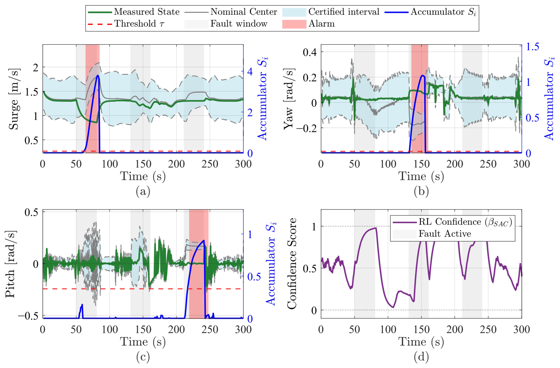
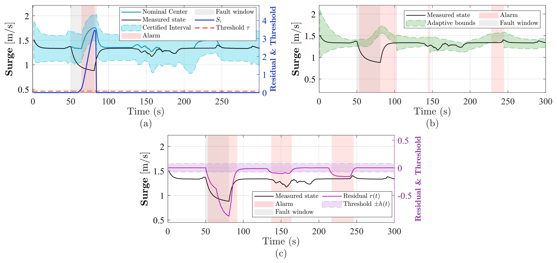
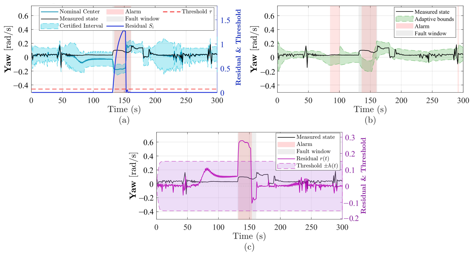
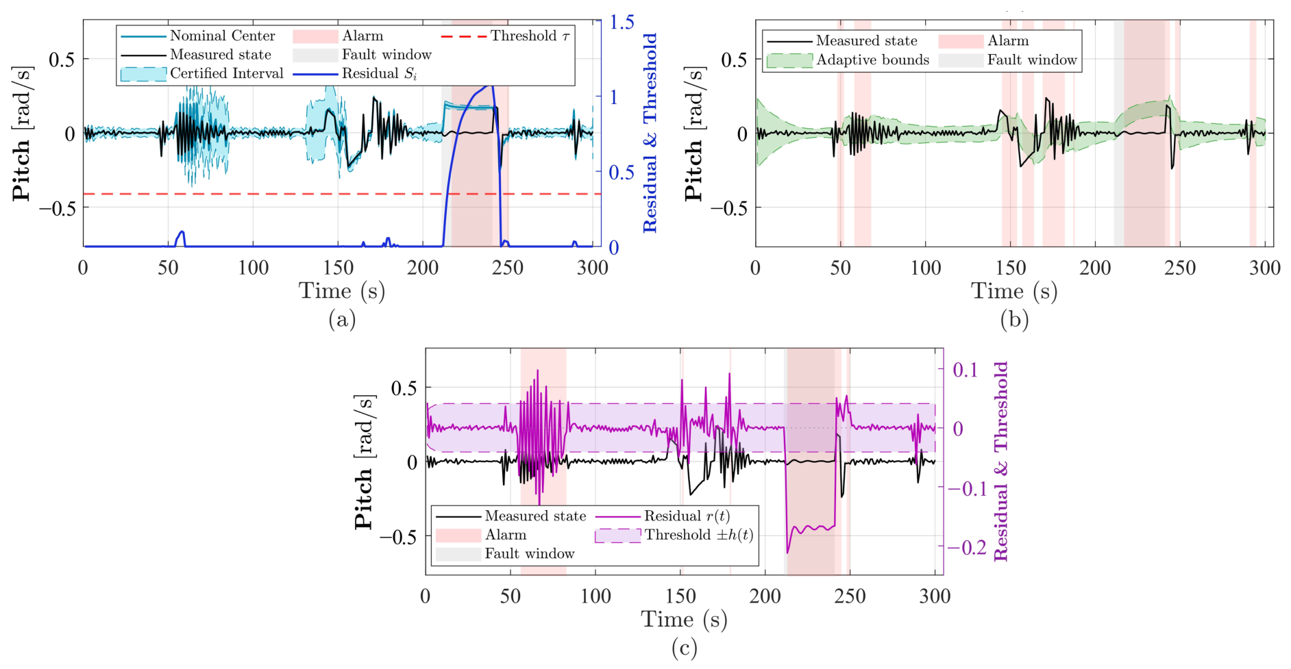
Sequential-fault performance is assessed under high uncertainty by examining healthy-state enclosure and channel-selective alarms. Figure 5 shows that all states remain enclosed within admissible intervals before fault onset. Confirmed alarms occur in the intended surge, yaw-rate, and pitch-rate channels with delays of 7, 6, and 5 s, respectively. No new alarm is raised during healthy operation after fault clearance. The $\beta \left(t\right)$ signal remains bounded while modulating the propagated tube slack.

Table 10. Sequential actuator-fault campaign after detector recovery update ($N=72$ scenario cases; all parameters fixed).

Metric	Surge (u)	Yaw (r)	Pitch (q)
Detection rate [%]	100.0	100.0	100.0
Detected events/total	72/72	72/72	72/72
Rising-edge false alarms	0	0	0
Delay [s]	$11.25\pm 2.16$	$3.60\pm 0.49$	$7.03\pm 1.49$
Delay range [s]	7–16	3–4	5–12
Post-clearance alarm tail [s]	$3.83$ mean, 5 max	$1.93$ mean, 8 max	$2.08$ mean, 8 max

Delays are measured on the 1 s IO-FDI diagnostic update grid. Rising-edge false alarms count new alarms outside active fault windows. Post-clearance tails are continuing alarms after a detected fault has vanished, not new false re-arms.

summarizes the aggregate performance of the sequential fault campaign.

5.3. Concurrent-Fault Isolation

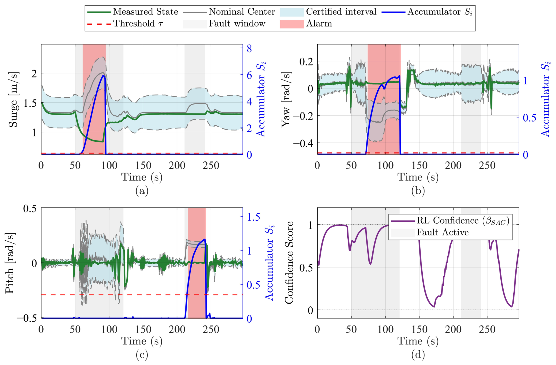
RAPIO is evaluated under overlapping surge and yaw faults to determine whether channel selectivity is preserved despite dynamic coupling. A surge fault is injected during $t=50$–90 s and a yaw fault during $t=70$–120 s, with a 20 s overlap ($t=70$–90 s). During the overlap, the cross-channel masking rule raises the yaw noise floor from $0.20$ to $0.60$ rad/s to suppress Coriolis-induced residuals. The yaw fault remains above the masked floor and therefore continues to increase the accumulator. Results over the full $N=72$ scenario grid are shown in Figure 6 and

Table 11. Concurrent fault isolation results under overlapping surge–yaw fault scenario ($N=72$ scenario cases; surge–yaw overlap window: $t=70$–90 s).

Metric	Surge (u)	Yaw (r)	Pitch (q)
Detection Rate [%]	100.0	100.0	100.0
FA/Case	0.00	0.00	0.00
Mean Delay [s]	$9.50\pm 1.69$	$4.29\pm 0.57$	$5.25\pm 1.02$
Yaw DR in overlap window [%]	—	100.0	—

.

Every fault is correctly isolated across all 72 scenarios, producing the correct FDI labels with zero false alarms. The mean yaw delay of $4.29$ s, despite the concurrent surge fault, confirms that the masked floor suppresses coupling residuals while remaining permeable to the genuine yaw signal.

5.4. Fault-Severity and Temporal-Profile Characterization

RAPIO is further assessed through severity and timing sweeps to establish when a fault produces sufficient evidence for confirmation. The 180-case sweep identifies the lowest LoE level confirmed in all six paired cases.

Table 12. Empirical LoE severity characterization (six paired cases per level).

Metric	Surge u	Yaw r	Pitch q
0% eventual-DR range	10–20%	10–60%	10–70%
Transition range	30–40%: 50% DR	—	80%: 16.7%; 90%: 50% DR
Minimum 100% eventual-DR level	50% LoE	70% LoE	100% LoE
DR at boundary	6/6	6/6	6/6
Mean delay [s]	11.33	4.00	6.83
False alarms	0	0	0

gives boundaries of 50% for surge, 70% for rudder, and 100% for the stern plane. Every case retained the Metzler certificate with no false alarms or cross-detections.

Below the complete-detection boundary, partial stern-plane losses were not confirmed in every paired condition because TNMPC can compensate them before a persistent interval inconsistency develops.

Table 13. Detection statistics for randomized and time-varying LoE profiles.

Channel and Profile	Eventual DR	Mean Delay [s]	FA/Cross
Surge—randomized abrupt	100.0%	11.50	0/0
Surge—gradual	100.0%	22.83	0/0
Surge—intermittent	50.0%	16.67	0/0
Yaw—randomized abrupt	100.0%	4.50	0/0
Yaw—gradual	83.3%	22.00	0/0
Yaw—intermittent	100.0%	3.00	0/0
Pitch—randomized abrupt	100.0%	6.00	0/0
Pitch—gradual	100.0%	24.00	0/0
Pitch—intermittent	100.0%	7.50	0/0
All channels and profiles	92.6%	—	0/0

reports six paired cases for each channel and profile, with mean delay computed over detected cases. Gradual-fault delay starts with the ramp, while intermittent detection is credited only during active degraded intervals. All 54 cases had no false alarms or cross-detections.

The missed cases are limited to intermittent surge and gradual yaw faults. Surge bursts of 6–7 s can end before sufficient evidence accumulates, after which the accumulator decays during the healthy gap. Gradual yaw loss begins near healthy operation and is initially absorbed by the closed-loop response. It is confirmed once the developing effect produces a sustained interval inconsistency, separating persistent faults from short recovery transients.

For 50% surge LoE,

Table 14. First-burst persistence characterization for intermittent 50% surge LoE.

Duration [s]	First-Burst Detection	Eventual Detection	Mean Delay [s]	Maximum Delay [s]
8	1/6	3/6	7.00	7
10	2/6	3/6	8.00	9
12	3/6	4/6	9.00	11
14	3/6	5/6	9.00	11
16	5/6	5/6	11.40	15
17	6/6	6/6	12.17	16
18	6/6	6/6	12.17	16

identifies 17 s as the shortest tested duration with 6/6 first-burst detections. The maximum delay was 16 s, and one case was not confirmed within a 16 s burst. Yaw faults were confirmed during 5–8 s bursts with a 3 s delay. Stern-plane faults used 7–8 s bursts and reached 100% eventual detection with a 7.5 s mean delay and a 5–16 s range. No false alarm or cross-detection occurred, and fault timing was not supplied to RAPIO.

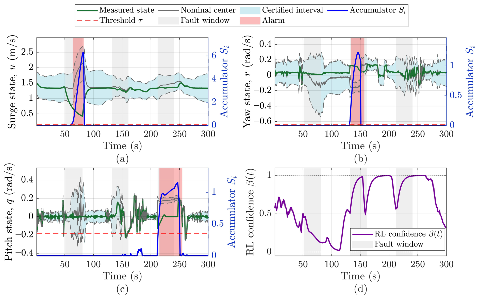
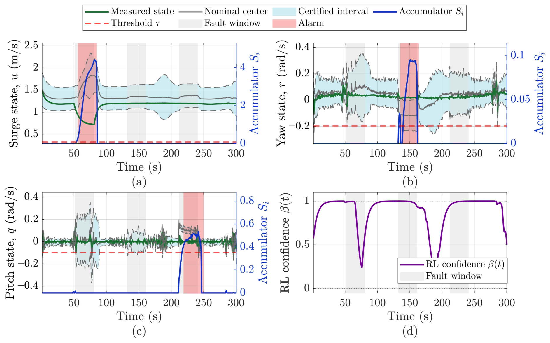
The evaluation is extended from LoE to additive bias and stuck/jam faults without changing RAPIO. Using Equation (16), these faults are applied only to the plant. The 18 jam events cover three channels, nominal and stressed conditions, and three seeds.

Table 15. Schedule-blind additive-bias and stuck/jam detection results (nominal and stressed environments, three seeds each; detector parameters unchanged).

Metric	Surge (u)	Yaw (r)	Pitch (q)
Nominal: last 0% bias DR	975 RPM	$7.5°$	$18°$
Nominal: first 100% bias DR	1300 RPM	$10°$	$22.5°$
Stressed: last 0% bias DR	325 RPM	$12.5°$	$18°$
Stressed: first 100% bias DR	487.5 RPM	$15°$	$22.5°$
Stuck/jam detections	6/6	6/6	6/6
Stuck/jam mean delay [s]	9.0	2.0	3.0

reports 18/18 detections and paired 100%-detection bias boundaries of 1300 RPM, $15°$, and $22.5°$. The biases are additive actuator offsets, and nominal surge also produced one detection at 1137.5 RPM. Across all 60 runs, no false alarms occurred and the Metzler certificate was retained. LoE is more demanding because it scales with the command and can be partly compensated by TNMPC, whereas bias persists and a jam breaks command tracking. Representative schedule-blind timelines appear in Figure 7 and Figure 8.

5.5. Comparative Benchmark Evaluation

RAPIO is benchmarked against a sign-based adaptive interval observer [25] and P2P threshold FDI [20] under identical conditions. All three methods use the same AUV dynamics, TNMPC controller, sensor noise, fault-injection protocol, and 72-case scenario grid. Figure 9, Figure 10 and Figure 11 compare the channel responses, and

Table 16. Three-method FDI benchmark over the common $N=72$ scenario cases. Each row gives the event count, detection rate, total healthy-time false-alarm events, and detection-delay distribution for one method–channel pair.

FDI Technique	Channel	Events	DR [%]	FA	Delay [s]
Proposed RAPIO	Surge (u)	72/72	100.0	0	$11.250\pm 2.161$
	Yaw (r)	72/72	100.0	0	$3.597\pm 0.494$
	Pitch (q)	72/72	100.0	0	$7.028\pm 1.491$
Adaptive IO [25]	Surge (u)	72/72	100.0	0	$3.000\pm 0.000$
	Yaw (r)	72/72	100.0	12	$6.486\pm 0.692$
	Pitch (q)	72/72	100.0	34	$9.153\pm 3.531$
P2P threshold FDI [20]	Surge (u)	72/72	100.0	9	$1.208\pm 1.198$
	Yaw (r)	54/72	75.0	0	$1.667\pm 0.476$
	Pitch (q)	72/72	100.0	4	$2.403\pm 0.781$

DR = event-level detection rate; FA = healthy-time alarm rising edges; delay is mean ± standard deviation over detected events.

summarizes the aggregate metrics. The adaptive-IO baseline transfers the reference method’s sign-based adaptive-bound mechanism to the actuator-sensitive AUV diagnostic channels. It therefore serves as a mechanism-level baseline; the original sensor-fault, linear-system application is not treated as equivalent to the present nonlinear actuator-fault problem.

The unchanged detector therefore identifies these command-path faults through persistent interval inconsistencies and characterizes the magnitude and persistence needed for confirmation.

Table 10 reports RAPIO’s channel-wise event counts, false alarms, and delay distributions, whereas Table 16 organizes the same metrics by method and channel for direct comparison.

The benchmark highlights a reliability–speed trade-off. RAPIO is not the fastest detector in surge or pitch, but it is the only method achieving $100\%$ detection on all three channels with zero event-level false alarms; the increased surge delay is the direct cost of this false-alarm immunity. The confirmation gate suppresses the Coriolis-induced transient residuals responsible for the 12 yaw and 34 pitch false alarms in the adaptive IO [25]. The P2P threshold FDI [20] responds faster but misses $25\%$ of yaw faults and retains 9 surge and 4 pitch false-alarm events.

RAPIO addresses the coupled AUV case through a bounded propagated tube. The physics-based envelope ${\mathit{\varphi }}_d\left(t\right)$ and the learned $\beta \left(t\right)$ modulate only the admissible width, while the scheduled gain and alarm thresholds remain fixed after calibration. The resulting detector favors persistent interval-consistency evidence over immediate threshold crossings; this increases the mean surge delay to $11.250\pm 2.161$ s, but avoids nuisance alarms under hydrodynamic uncertainty and coupled surge–yaw–pitch motion. Across the completed sequential-fault campaign, RAPIO detected all 216 injected fault events without producing an alarm rising edge outside an active fault window.

6. Discussion

The central strength of RAPIO lies in allowing uncertainty bounds to adapt while keeping the diagnostic logic physically interpretable and verifiable. This separation places the method between conservative fixed-bound interval observers and fully adaptive decision rules. A fixed worst-case envelope can preserve inclusion, but it often produces an unnecessarily wide tube. Directly adapting the residual thresholds creates a different concern because coupled transients may then influence the fault decision. RAPIO balances these effects by restricting the learned signal $\beta \left(t\right)$ to a bounded adjustment of the tube slack. The nominal center, scheduled gain, Metzler/Hurwitz certificate, and alarm gates remain model-based. Consequently, learning regulates the admissible uncertainty without changing either the physical interpretation of a fault or the conditions used to verify fault-free interval inclusion.

The common-grid benchmark in Table 16 supports this design choice. Among the compared methods, only RAPIO achieves complete detection in all three channels without event-level false alarms. P2P responds more quickly, but it misses yaw faults and produces false alarms in the surge and pitch channels. The adaptive IO detects all faults, although nuisance alarms remain in the coupled yaw and pitch channels. RAPIO’s longer surge delay has a different origin from a general computational delay. TNMPC initially attenuates the propulsion mismatch, and the persistence gate confirms the event after the tube violation becomes sustained. This behavior favors reliable isolation in long-duration AUV operation, where a transient departure may also accompany ordinary disturbance recovery.

The fault-characterization campaigns further show that detectability depends on fault magnitude, temporal development, and closed-loop sensitivity. The channel boundaries in Table 12 arise from differences in control authority and hydrodynamic coupling. Partial losses can remain compensated until their effect on the monitored state exceeds the admissible tube. This behavior also explains the influence of the fault profile. A gradual fault needs time to develop a persistent signature, whereas the healthy gaps in an intermittent profile allow accumulated evidence to decay. For the tested 50% LoE surge cases, Table 14 shows that a 17 s active-fault duration was sufficient for full first-burst detection. By contrast, additive bias and jammed actuation create sustained disagreement between the commanded and realized response. The unchanged detector therefore confirms every tested stuck/jam event and the full-detection bias boundaries reported in Table 15. These results show that the same interval-consistency logic responds to distinct command-path fault structures without receiving the fault schedule or class.

Taken together, the analytical and simulation results define a clear operating domain for RAPIO. The evaluation covers a nonlinear 6-DOF plant, bounded-error FTESO reconstruction, paired control-surface actuation, large hydrodynamic variation, current disturbances, and multiple seeded fault profiles. Within this setting, the model-based certificate establishes fault-free enclosure under the stated disturbance and local-freezing assumptions. The severity and persistence sweeps complement that result by identifying the demonstrated detection domain. Hardware-in-the-loop testing is the next stage for evaluating real-time implementation effects. The present fault scope covers LoE, additive-bias, and stuck/jammed command-path faults. Actuator-dynamics and hydrodynamic-parameter faults require extended actuator and parameter-estimation models.

7. Conclusions

This paper presented a robust adaptive propagated interval observer (RAPIO) for actuator fault detection and isolation in underactuated AUVs under bounded disturbances and hydrodynamic uncertainty. RAPIO combines a Metzler-certified interval observer, Van Loan width propagation, interval-consistency residuals, and a fixed-threshold leaky decision layer. Reinforcement learning supplies the bounded scalar signal $\beta \left(t\right)$ that modulates the admissible uncertainty width.

Under the stated assumptions, separating learning from the observer core preserves positivity and interval inclusion. The scheduled observer matrix remains Metzler and Hurwitz, while the half-width dynamics remain positive and uniformly ultimately bounded. The true state also remains enclosed in the fault-free case. The certified tube supports channel-wise violations, persistence confirmation, and recovery logic for surge, yaw-rate, and pitch-rate actuator fault isolation under LoE, additive-bias, and stuck/jammed actuation.

Across 72 severe sequential-fault cases spanning $\pm 50\%$ hydrodynamic variation and $0.3\mathrm{m}/\mathrm{s}$ base currents with time-varying, depth-shear, and spatial components, together with the additional severity, timing, bias, and stuck/jam campaigns, RAPIO produced no false alarms. It detected every fault in the 72-case sequential campaign and all 18 stuck/jam events. Mean surge, yaw-rate, and pitch-rate detection delays in the 72-case sweep were 11.25, 3.60, and 7.03 s, respectively. Against the adaptive IO [25] and P2P threshold FDI [20], RAPIO achieved the strongest reliability profile, with $100\%$ detection on all channels and zero event-level false alarms. In contrast, the baselines produced yaw/pitch false alarms or missed yaw faults.

These results support RAPIO as a safety-oriented diagnostic layer for long-duration AUV missions, where false alarms can be more disruptive than modest confirmation delays. Future work will address degraded sensing, joint actuator–sensor diagnosis, fault-tolerant control, and hardware-in-the-loop validation.

References

1. Liu, C.; Filaretov, V.; Zuev, A.; Protsenko, A.; Zhirabok, A. Fault tolerant control in underwater vehicles. J. Mar. Sci. Eng. 2024, 12, 1836. [Google Scholar] [CrossRef]
2. Wang, Y.; Yu, G.; Xie, W.; Zhang, W.; Silvestre, C. Cooperative path following control of a team of Quadrotor-Slung-Load Systems under disturbances. IEEE Trans. Intell. Veh. 2023, 8, 4169–4179. [Google Scholar] [CrossRef]
3. Shan, Y.; Zhu, F. Interval observer-based fault tolerant control strategy with fault estimation and compensation. Asian J. Control 2022, 24, 895–906. [Google Scholar] [CrossRef]
4. Hao, L.Y.; Yang, X.; Zhang, Y.Q.; Atajan, H.; Liu, Y. Fault-tolerant control of unmanned marine vehicles with unknown parametric dynamics via integral sliding mode output feedback control. Asian J. Control 2025, 27, 840–851. [Google Scholar] [CrossRef]
5. Zhou, M.; Li, H.; Wang, J.; Raïssi, T. Event-triggered H-fault-tolerant consistency control for multi-agent systems. Eur. J. Control 2024, 79, 101083. [Google Scholar] [CrossRef]
6. Gao, Z.; Cecati, C.; Ding, S.X. A Survey of Fault Diagnosis and Fault-Tolerant Techniques—Part I: Fault Diagnosis with Model-Based and Signal-Based Approaches. IEEE Trans. Ind. Electron. 2015, 62, 3757–3767. [Google Scholar] [CrossRef]
7. Lan, J.; Patton, R.J. Robust Integration of Model-Based Fault Estimation and Fault-Tolerant Control; Springer Nature: Cham, Switzerland, 2021. [Google Scholar] [CrossRef]
8. Chanthery, E.; Travé-Massuyès, L.; Indra, S. Fault isolation on request based on decentralized residual generation. IEEE Trans. Syst. Man Cybern. Syst. 2016, 46, 598–610. [Google Scholar] [CrossRef]
9. Blanke, M.; Kinnaert, M.; Lunze, J.; Staroswiecki, M. Diagnosis and Fault-Tolerant Control; Springer Series in Control Engineering; Springer: Berlin/Heidelberg, Germany, 2006. [Google Scholar]
10. Efimov, D.; Raïssi, T. Design of Interval Observers for Uncertain Dynamical Systems. Autom. Remote Control 2016, 77, 191–225. [Google Scholar] [CrossRef]
11. Raïssi, T.; Ramdani, N.; Candau, Y. Set Membership State and Parameter Estimation for Systems Described by Nonlinear Differential Equations. Automatica 2004, 40, 1771–1777. [Google Scholar] [CrossRef]
12. Chevet, T.; Dinh, T.N.; Marzat, J.; Raïssi, T. Robust Sensor Fault Detection for Linear Parameter-Varying Systems using Interval Observer. In Proceedings of the 31st European Safety and Reliability Conference, Angers, France, 19–23 September 2021; pp. 1486–1493. [Google Scholar] [CrossRef]
13. Akremi, R.; Lamouchi, R.; Amairi, M.; Dinh, T.N.; Raïssi, T. Functional interval observer design for multivariable linear parameter-varying systems. Eur. J. Control 2023, 71, 100794. [Google Scholar] [CrossRef]
14. Mizouri, H.; Lamouchi, R.; Amairi, M.; Raissi, T. Functional Interval Observers-Based Fault-Tolerant Control for Linear Parameter-Varying Systems. Int. J. Robust Nonlinear Control 2026, 36, 155–171. [Google Scholar] [CrossRef]
15. Li, J.; Wang, Z.; Raïssi, T.; Shen, Y. Unknown Input Observer Design for Linear Parameter-Varying Systems in a Bounded Error Context. IEEE Trans. Autom. Control 2021, 66, 4246–4251. [Google Scholar] [CrossRef]
16. Zhang, Z.H.; Yang, G.H. Distributed fault detection and isolation for multiagent systems: An interval observer approach. IEEE Trans. Syst. Man Cybern. Syst. 2020, 50, 2220–2230. [Google Scholar] [CrossRef]
17. Zhang, R.; Wang, Z.; Meslem, N.; Raïssi, T.; Shen, Y. Fault Detection for Lipschitz Nonlinear Systems Using Robust Observer and Ellipsoidal Analysis. Int. J. Robust Nonlinear Control 2025, 35, 4523–4535. [Google Scholar] [CrossRef]
18. Zhu, F.; Fu, Y.; Dinh, T.N. Asymptotic convergence unknown input observer design via interval observer. Automatica 2023, 147, 110744. [Google Scholar] [CrossRef]
19. Zhu, F.; Li, M. Distributed Interval Observer and Distributed Unknown Input Observer Designs. IEEE Trans. Autom. Control 2024, 69, 8868–8875. [Google Scholar] [CrossRef]
20. Ma, Y.; Wang, Z.; Meslem, N.; Raïssi, T.; Shen, Y. Fault diagnosis by interval-based adaptive thresholds and peak-to-peak observers. Int. J. Adapt. Control Signal Process. 2023, 37, 519–537. [Google Scholar] [CrossRef]
21. Tian, M.; Guo, Z.; Wang, X.; Niu, B.; Wang, X.; Wang, D.; Wang, H. Fault Detection and Isolation for Multiagent Systems Under Event-Triggered Communication: A Zonotopic Joint Estimation Method. IEEE Internet Things J. 2025, 12, 29940–29947. [Google Scholar] [CrossRef]
22. Zhu, X.; Li, Y.; Yin, G.; Patton, R.J. Interval Observer-Based Fault Detection and Isolation for Quadrotor UAV With Cable-Suspended Load. IEEE Trans. Syst. Man Cybern. Syst. 2024, 54, 5876–5888. [Google Scholar] [CrossRef]
23. Guzmán-Rabasa, J.; Rodríguez, F.; Valencia-Palomo, G.; Santos-Ruiz, I.; Gómez-Peñate, S.; López-Estrada, F.R. Convex Fault Diagnosis of a Three-Degree-of-Freedom Mechanical Crane. Mathematics 2023, 11, 4258. [Google Scholar] [CrossRef]
24. Song, J.; He, X. Robust state estimation and fault detection for Autonomous Underwater Vehicles considering hydrodynamic effects. Control Eng. Pract. 2023, 135, 105497. [Google Scholar] [CrossRef]
25. Wang, X.; Pin Tan, C.; Wang, Y.; Zhang, Z. Active fault tolerant control based on adaptive interval observer for uncertain systems with sensor faults. Int. J. Robust Nonlinear Control 2021, 31, 2857–2881. [Google Scholar] [CrossRef]
26. Yan, Z.; Xu, F.; Tan, J.; Liu, H.; Liang, B. Reinforcement learning-based integrated active fault diagnosis and tracking control. ISA Trans. 2023, 132, 364–376. [Google Scholar] [CrossRef] [PubMed]
27. Ali, S.M.; Rabbani, T.; Bilal, M.; Alharbi, A.; Aldosari, F.M.; Amin, R.U. Dynamics Estimation and Deep Reinforcement Learning based Fractal Inspired Sliding Mode Control of Stewart Platform. Results Control Optim. 2026, 100779. [Google Scholar] [CrossRef]
28. Li, Z.; Wang, M.; Ma, G.; Zou, T. Adaptive reinforcement learning fault-tolerant control for AUVs with thruster faults based on the integral extended state observer. Ocean Eng. 2023, 271, 113722. [Google Scholar] [CrossRef]
29. Jmal, A.; Naifar, O.; Ben Makhlouf, A.; Derbel, N.; Hammami, M.A. Observer-based model reference control for linear fractional-order systems. Int. J. Digit. Signals Smart Syst. 2018, 2, 136–149. [Google Scholar] [CrossRef]
30. Naifar, O.; Jmal, A.; Ben Makhlouf, A.; Derbel, N.; Hammami, M.A. Observer-based control for fractional-order systems. In Fractional Order Systems—Control Theory and Applications: Fundamentals and Applications; Springer: Cham, Switzerland, 2021; pp. 75–93. [Google Scholar] [CrossRef]
31. Jmal, A.; Naifar, O.; Rhaima, M.; Ben Makhlouf, A.; Mchiri, L. On Observer and Controller Design for Nonlinear Hadamard Fractional-Order One-Sided Lipschitz Systems. Fractal Fract. 2024, 8, 606. [Google Scholar] [CrossRef]
32. Alsharif, A.O.M.; Jmal, A.; Naifar, O.; Ben Makhlouf, A.; Rhaima, M.; Mchiri, L. Unknown Input Observer Scheme for a Class of Nonlinear Generalized Proportional Fractional Order Systems. Symmetry 2023, 15, 1233. [Google Scholar] [CrossRef]
33. Ahmed, H.; Jmal, A.; Ben Makhlouf, A. A practical observer for state and sensor fault reconstruction of a class of fractional-order nonlinear systems. Eur. Phys. J. Spec. Top. 2023, 232, 2437–2443. [Google Scholar] [CrossRef]
34. Fossen, T.I. Handbook of Marine Craft Hydrodynamics and Motion Control; John Wiley & Sons: Chichester, UK, 2011. [Google Scholar]
35. Wang, Z.; Shen, Y. Model-Based Fault Diagnosis: Methods for State-Space Systems; Studies in Systems, Decision and Control; Springer: Singapore, 2023; Volume 221. [Google Scholar] [CrossRef]
36. Prestero, T. Development of a six-degree of freedom simulation model for the REMUS autonomous underwater vehicle. In Proceedings of the MTS/IEEE Oceans 2001. An Ocean Odyssey. Conference Proceedings (IEEE Cat. No.01CH37295), Honolulu, HI, USA, 5–8 November 2001; Volume 1, pp. 450–455. [Google Scholar] [CrossRef]
37. Mazenc, F.; Bernard, O. Interval observers for linear time-invariant systems with disturbances. Automatica 2011, 47, 140–147. [Google Scholar] [CrossRef]
38. Haarnoja, T.; Zhou, A.; Abbeel, P.; Levine, S. Soft Actor-Critic: Off-Policy Maximum Entropy Deep Reinforcement Learning with a Stochastic Actor. In Proceedings of the 35th International Conference on Machine Learning; Dy, J., Krause, A., Eds.; PMLR: New York, NY, USA, 2018; Volume 80, pp. 1861–1870. [Google Scholar]
Figure 1. Underactuated AUV showing the NED and body-fixed frames, ocean-current velocity, body-motion variables, and actuator force/moment channels.
Jmse 14 01445 g001
Figure 2. Proposed RAPIO-based FDI architecture. The labeled shared-command branch shows that the same actuator command u ( t ) is supplied to the AUV plant, FTESO, and observer state propagation. The plant/reconstructor output y ( t ) , FTESO disturbance estimate d ^ ( t ) , interval bounds, and learned modulation β ( t ) are separate signals.
Jmse 14 01445 g002
Figure 3. RL-augmented bound modulation architecture. The RAPIO observer receives a bounded scalar modulation signal β ( t ) from the learned supervisory policy. This signal modulates only the slack term in the interval width dynamics, while the scheduled-gain rule and nominal center predictor remain fixed.
Jmse 14 01445 g003
Figure 4. Online RAPIO propagation and fault-decision process. The frozen SAC policy modulates only the interval-width slack; the locally frozen model, fixed scheduled-gain rule, and center dynamics remain independent of learning.
Jmse 14 01445 g004
Figure 5. Sequential actuator-fault detection for (a) surge, (b) yaw-rate, and (c) pitch-rate channels under RL–RAPIO interval-consistency monitoring; (d) learned confidence β ( t ) .
Jmse 14 01445 g005
Figure 6. Concurrent surge–yaw faults followed by a pitch fault, showing channel-wise isolation in (a) surge, (b) yaw rate, and (c) pitch rate; (d) learned confidence β ( t ) .
Jmse 14 01445 g006
Figure 7. Schedule-blind RAPIO response to detected additive actuator-bias faults: (a) surge, (b) yaw, (c) pitch, and (d) learned confidence β ( t ) .
Jmse 14 01445 g007
Figure 8. Schedule-blind RAPIO response to detected stuck/jammed actuator faults: (a) surge, (b) yaw, (c) pitch, and (d) learned confidence β ( t ) .
Jmse 14 01445 g008
Figure 9. Surge-channel benchmark: (a) RAPIO, (b) adaptive IO [25], and (c) P2P threshold FDI [20].
Jmse 14 01445 g009
Figure 10. Yaw-rate-channel benchmark: (a) RAPIO, (b) adaptive IO [25], and (c) P2P threshold FDI [20].
Jmse 14 01445 g010
Figure 11. Pitch-channel benchmark: (a) RAPIO, (b) adaptive IO [25], and (c) P2P threshold FDI [20].
Jmse 14 01445 g011