Soft-Gating Mixture Robust Kalman Filter for SINS/DVL Integrated Navigation Under DVL Outlier Interference

Abstract

Aiming at the problem that complex underwater environments induce outliers in Doppler Velocity Log (DVL) measurements, which degrade the navigation accuracy of the Strapdown Inertial Navigation System (SINS)/DVL integrated system, this paper proposes a soft-gating Gaussian–Student’s t mixture robust Kalman filter (MRKF). Firstly, the measurement noise is modeled as a mixture of Gaussian and Student’s t distributions to adapt to normal stationary noise and abrupt outliers, respectively. Secondly, a logistic soft-gating weight is constructed based on the innovation Mahalanobis distance to adaptively balance the output contributions of the standard Kalman Filter (KF) and the variational Bayesian Student’s t filter. Finally, moment matching is adopted to realize the weighted fusion of two-branch posterior distributions, and an equivalent Gaussian posterior estimation is obtained. Simulation results under the considered SINS/DVL integrated navigation scenarios show that the proposed MRKF maintains estimation accuracy close to the standard KF under nominal Gaussian measurement noise. In the designed DVL outlier-injection scenario, the proposed MRKF achieves a position RMSE of $53.39\mathrm{m}$, compared with $878.75\mathrm{m}$, $58.84\mathrm{m}$, and $56.49\mathrm{m}$ for the nominal KF, Huber KF (HKF), and Student’s-t variational Bayesian KF (STVBKF), respectively. These results indicate that the proposed MRKF can improve robustness against DVL outliers while maintaining competitive estimation accuracy under the simulated conditions.

1. Introduction

The strapdown inertial navigation system (SINS) acquires inertial measurements of the carrier in real time using gyroscopes and accelerometers, and calculates the attitude, velocity, and position of the carrier. Featuring excellent navigation continuity and high short-term positioning accuracy, SINS has become an essential device for autonomous navigation [1,2,3]. The Doppler Velocity Log (DVL) can directly measure the seabed-referenced velocity of underwater carriers, and its velocity error does not accumulate over time, which effectively suppresses the long-term error drift of SINS [4,5]. Accordingly, the SINS/DVL integrated navigation system combines the complementary advantages of SINS and DVL, and  has evolved into a mainstream navigation scheme for autonomous underwater vehicles (AUVs) [6,7]. Nevertheless, the complicated and variable underwater environment inevitably induces ocean current disturbances, seabed undulations, and acoustic refraction, thereby generating abrupt outliers and non-Gaussian anomalies in DVL measurements. Such abnormal disturbances severely degrade the estimation accuracy and stability of the SINS/DVL integrated navigation system [8,9]. Therefore, the investigation of robust filtering algorithms tailored for SINS/DVL systems is of practical engineering significance for improving the navigation reliability of underwater vehicles.

At present, existing robust filtering methods for outlier suppression can be broadly categorized into two types: M-estimation and statistical modeling. In 1964, Huber combined the characteristics of L1-norm and L2-norm influence functions and proposed a classical Huber cost function. By replacing the original L2-norm cost function in the Kalman filter, an M-estimation-based robust filtering framework was established, providing a fundamental solution for outlier suppression [10,11]. On this basis, subsequent researchers have introduced various robust criteria into the Kalman filter, further expanding the application scope of M-estimation-based robust filtering methods [12,13]. In recent years, statistical modeling methods based on the Student’s t-distribution have attracted widespread attention. Owing to its heavy-tailed feature and redescending influence function, the Student’s t-distribution can naturally characterize non-Gaussian heavy-tailed noise. Accordingly, variational Bayesian (VB) Student’s t robust filtering has been gradually applied in the integrated navigation field [14,15,16,17,18] and has been successfully implemented in various integrated navigation systems such as SINS/global navigation satellite system (GNSS) [19,20]. Nevertheless, existing single robust filtering algorithms still suffer from obvious limitations. Specifically, M-estimation relies on fixed thresholds and exhibits poor adaptability to weak abnormal disturbances, resulting in limited robustness. In addition, the Student’s t filter excessively fits heavy-tailed noise and inevitably sacrifices estimation accuracy under pure Gaussian noise conditions. Therefore, a single robust filter cannot simultaneously satisfy the dual requirements of high accuracy under normal conditions and strong robustness under abnormal interference for SINS/DVL integrated navigation systems.

To address the above issues, this paper proposes a soft-gating Gaussian–Student’s t mixture robust Kalman filter (MRKF). In the proposed MRKF, DVL measurement noise is modeled as a mixture of Gaussian and Student’s t distributions to adapt to steady Gaussian noise and abrupt outliers, respectively. Furthermore, a logistic soft-gating weight is constructed based on the innovation Mahalanobis distance to adaptively balance the output weights of the standard Kalman filter and the variational Bayesian Student’s t filter. Subsequently, a moment matching strategy is adopted to fuse the posterior distributions from the two branches and generate equivalent Gaussian posterior estimates, realizing the integration of high accuracy under normal conditions and strong robustness under abnormal interference. The simulation results demonstrate that the proposed MRKF achieves superior comprehensive performance compared with conventional robust filtering methods, which can effectively improve the navigation accuracy and stability of SINS/DVL integrated navigation systems in complex underwater environments.

The main contributions of this paper are summarized as follows:

• Gaussian–Student’s t mixture noise model is established to simultaneously fit normal Gaussian noise and abrupt DVL outliers, breaking through the limitations of single noise assumption.
• An innovation Mahalanobis distance-driven soft-gating mechanism is designed in the proposed MRKF to realize the adaptive smooth switching between the standard Kalman filter and the Student’s t-based robust filter, which avoids estimation mutations caused by rigid thresholds.
• A dual-branch posterior moment-matching fusion strategy is proposed to output equivalent Gaussian estimates. The proposed MRKF maintains high precision under normal conditions and achieves strong robustness against abnormal outliers, making it suitable for complex underwater SINS/DVL navigation scenarios.

The remainder of this paper is organized as follows. Section 2 elaborates the research background of SINS/DVL integrated navigation and the fundamentals of noise modeling, clarifying the limitations of conventional filtering methods. In Section 3, the proposed MRKF is comprehensively derived. Section 4 conducts multi-condition simulation experiments to quantitatively compare the navigation performance of the proposed algorithm with several typical existing robust filters. Finally, Section 5 concludes this paper and presents potential future research directions.

2. SINS/DVL Integrated Navigation Model and Problem Analysis

2.1. Navigation Sensor Output Model

SINS/DVL integrated navigation is one of the dominant navigation approaches for underwater AUVs. Establishing a state-space model and adopting the Kalman filter for data fusion is a typical implementation of SINS/DVL integrated navigation. The constructed state-space model consists of the SINS kinetic equation and the DVL measurement output model. Generally, the error-state equations of SINS can be expressed as follows [7]:

$${\dot{\mathit{\varphi }}}^{\mathbf{n}}=-{\omega }_{in}^n\times {\mathit{\varphi }}^n-{\mathbf{C}}_b^n\delta {\omega }_{ib}^b+\delta {\omega }_{in}^n$$

(1)

$$\delta {\dot{\mathbf{v}}}^n=\left({\mathbf{C}}_b^n{\tilde{\mathbf{f}}}^b\right)\times {\mathit{\varphi }}^n-(2{\omega }_{ie}^n+{\omega }_{en}^n)\times \delta {\mathbf{v}}^n+{\tilde{\mathbf{v}}}^n\times (2\delta {\omega }_{ie}^n+\delta {\omega }_{en}^n)+{\mathbf{C}}_b^n\delta {\mathbf{f}}^{\mathbf{b}}$$

(2)

$$\delta \dot{\mathbf{p}}={\mathbf{M}}_{pv}\delta {\mathbf{v}}^n+{\mathbf{M}}_{pp}\delta \mathbf{p}$$

(3)

where n, b, i, and e denote the east-north-up navigation frame, the body frame, the inertial frame, and the Earth frame, respectively. ${\mathbf{C}}_b^n$ denotes the coordinate transformation matrix from the body frame to the navigation frame. ${\omega }_{xy}^z$ denotes the projection, in the z frame, of the angular velocity of the y frame with respect to the x frame, and $\delta {\omega }_{xy}^z$ denotes the corresponding angular velocity error. ${\mathbf{v}}^n$ and ${\mathbf{p}}^n$ are the projections of the velocity vector and the position vector in the navigation frame, respectively. ${\mathit{\varphi }}^n$, $\delta {\mathbf{v}}^n$, and $\delta {\mathbf{p}}^n$ denote the attitude error vector, velocity error vector, and position error vector, respectively. ${\tilde{\mathbf{f}}}^b$ and ${\tilde{\omega }}_{ib}^b$ denote the specific force and angular velocity measured by the accelerometer and gyroscope, respectively. ${\mathbf{M}}_{pv}$ and ${\mathbf{M}}_{pp}$ denote the coefficient matrices of the velocity error vector and the position error vector in the position error equation, respectively.

$\delta {\omega }_{ib}^b$ and $\delta {\mathbf{f}}^b$ denote the output errors of the gyroscope and accelerometer, respectively, which can generally be expressed as:

$$\delta {\omega }_{ib}^b={\tilde{\omega }}_{ib}^b-{\omega }_{ib}^b={\epsilon }^b+{\mathbf{n}}^g$$

(4)

$$\delta {\mathbf{f}}^b={\tilde{\mathbf{f}}}^b-{\mathbf{f}}^b={\nabla }^b+{\mathbf{n}}^a$$

(5)

In the above equation, ${\epsilon }^b$ and ${\nabla }^b$ denote the gyroscope constant drift and accelerometer bias, respectively, which can generally be modeled as constant-value models. ${\mathbf{n}}_g^b$ and ${\mathbf{n}}_a^b$ denote the random noise of the gyroscope output and the random noise of the accelerometer, respectively.

Considering the case where the lever arm and installation misalignment angles have been calibrated, the DVL output error equation can be expressed as ${\tilde{\mathbf{v}}}_{dvl}^b$:

$${\tilde{\mathbf{v}}}_{dvl}^b=\left(1+\delta k\right)·{\mathbf{v}}^b+{\mathbf{n}}_d$$

(6)

where ${\mathbf{n}}_d$ denotes the DVL output noise, which ideally follows a zero-mean Gaussian distribution. $\delta k$ denotes the scale factor error, which does not vary rapidly over a short period of time and therefore can be modeled as a constant-value model:

$$\delta \dot{k}=0$$

(7)

By taking the difference between the DVL output and the velocity calculated by the SINS, the measurement equation of the integrated navigation system can be established as

$$\begin{array}{c}{\mathbf{z}}_{dvl}={\left({\tilde{\mathbf{C}}}_b^n\right)}^T{\tilde{\mathbf{v}}}^n-{\tilde{\mathbf{v}}}_{dvl}^b\hfill \\ ={\left({\mathbf{C}}_b^n\right)}^T\left(\mathbf{I}+{\mathit{\varphi }}^{\mathbf{n}}\times \right)\left({\mathbf{v}}^n+\delta {\mathbf{v}}^n\right)-\left(1+\delta k\right)·{\mathbf{v}}^b-{\mathbf{n}}_d\hfill \\ =-{\left({\mathbf{C}}_b^n\right)}^T\left({\tilde{\mathbf{v}}}^n\times \right)\mathit{\varphi }+{\left({\mathbf{C}}_b^n\right)}^T\delta {\mathbf{v}}^n-\delta k·{\mathbf{v}}^b-{\mathbf{n}}_d\hfill \end{array}$$

(8)

2.2. The Problem Statement

The state vector of the integrated navigation system is selected as:

$${\mathbf{x}}_{ins}={\left[\begin{array}{cccccc}{\left({\mathit{\varphi }}^n\right)}^T& {\left(\delta {\mathbf{v}}^n\right)}^T& \delta {\mathbf{p}}^T& {\left({\epsilon }^b\right)}^T& {\left({\nabla }^b\right)}^T& \delta k\end{array}\right]}^T$$

(9)

According to (1)–(3), the system model of the integrated navigation system can be established as:

$${\dot{\mathbf{x}}}_{ins}={\mathbf{F}}_{ins}{\mathbf{x}}_{ins}+{\mathbf{G}}_{ins}{\mathbf{w}}_{ins}$$

(10)

where ${\mathbf{F}}_{\mathrm{ins}}$ is the state transition matrix, ${\mathbf{G}}_{\mathrm{ins}}$ is the system noise driving matrix, and ${\mathbf{w}}_{\mathrm{ins}}$ is the process noise. By rearranging (8) into matrix form, the linear measurement model can be obtained as:

$${\mathbf{z}}_{dvl}={\mathbf{H}}_{dvl}\mathbf{x}+{\mathbf{n}}_{dvl}$$

(11)

where

$${\mathbf{H}}_{dvl}=\left[\begin{array}{cccc}-{\left({\mathbf{C}}_b^n\right)}^T\left({\tilde{\mathbf{v}}}^n\times \right)& {\left({\mathbf{C}}_b^n\right)}^T& {\mathbf{0}}_{3\times 9}& -{\mathbf{v}}^b\end{array}\right]$$

(12)

The continuous-time SINS error-state propagation model in (10) and the DVL measurement model in (11) are combined and discretized to obtain the following discrete linear state-space model:

$$\begin{array}{c}{\mathbf{x}}_k={\mathrm{\Phi }}_{k-1}{\mathbf{x}}_{k-1}+{\mathrm{\Gamma }}_{k-1}{\mathbf{w}}_{k-1}\hfill \\ {\mathbf{z}}_k={\mathbf{H}}_k{\mathbf{x}}_k+{\mathbf{v}}_k\hfill \end{array}$$

(13)

where

$${\mathrm{\Phi }}_{k-1}\approx \mathbf{I}+{\mathbf{F}}_{ins}\left(t_{k-1}\right)T$$

$${\mathrm{\Gamma }}_{k-1}\approx \left({\mathbf{I}}_T+{\mathbf{F}}_{ins}\left(t_{k-1}\right){\displaystyle \frac{T^2}{2}}\right){\mathbf{G}}_{ins}\left(t_{k-1}\right)$$

$${\mathbf{H}}_k={\mathbf{H}}_{dvl}$$

The process noise ${\mathbf{w}}_k$ satisfies ${\mathbf{w}}_k\sim \mathcal{N}(\mathbf{0},{\mathbf{Q}}_k)$. In the conventional Kalman filter, the measurement noise ${\mathbf{v}}_k$ is assumed to satisfy ${\mathbf{v}}_k\sim \mathcal{N}(\mathbf{0},{\mathbf{R}}_k)$. ${\mathbf{Q}}_k$ denotes the nominal process noise covariance matrix, and ${\mathbf{R}}_k$ denotes the nominal measurement noise covariance matrix. In the SINS/DVL error-state filtering framework, the inertial measurements from gyroscopes and accelerometers are used for state propagation, while the DVL velocity measurement is used for measurement correction. When DVL outliers occur, large innovations may be directly introduced into the state update through the Kalman gain, thereby contaminating the velocity, attitude, and position-error estimates. Therefore, the main problem addressed in this paper is the robust measurement update of the SINS/DVL error-state filter under abnormal DVL interference. To balance the estimation accuracy under normal conditions and the robustness under abnormal conditions, the proposed MRKF is constructed in this paper.

3. Design and Derivation of the Soft-Gating Gaussian–Student’s t MRKF

The basic idea of the proposed MRKF is as follows: at each filtering time step, the measurement update under the standard Kalman filter and the robust update based on the Student’s-t heavy-tailed noise assumption are computed simultaneously. Then, a soft-gating weight is designed according to the innovation statistic to perform weighted fusion of the two posterior distributions, and moment matching is employed to obtain the final equivalent Gaussian posterior distribution.

3.1. Construction of the Soft-Gating Weight Based on the Innovation Statistic

For the SINS/DVL integrated navigation system model, its one-step predictive probability density function can be modeled as a Gaussian distribution:

$$p\left({\mathbf{x}}_k\right|{\mathbf{z}}_{1:k-1})=\mathrm{N}({\mathbf{x}}_k;{\hat{\mathbf{x}}}_{k|k-1},{\mathbf{P}}_{k|k-1})$$

(14)

According to the integrated navigation model in (13) and the one-step predictive probability density function model in (14), the corresponding one-step prediction update process can be obtained as follows:

$${\hat{\mathbf{x}}}_{k|k-1}={\mathrm{\Phi }}_{k-1}{\hat{\mathbf{x}}}_{k-1}$$

(15)

$${\mathbf{P}}_{k|k-1}={\mathrm{\Phi }}_{k-1}{\mathbf{P}}_{k-1}{\mathrm{\Phi }}_{k-1}^T+{\mathrm{\Gamma }}_{k-1}{\mathbf{Q}}_{k-1}{\mathrm{\Gamma }}_{k-1}^T$$

(16)

In the above equation, ${\hat{\mathbf{x}}}_{k-1}$ and ${\mathbf{P}}_{k-1}$ denote the estimated state and the error covariance matrix at filtering time step $k-1$, respectively. Given the predicted state ${\hat{\mathbf{x}}}_{k|k-1}$, the predicted measurement can be obtained as:

$${\hat{\mathbf{z}}}_{k|k-1}={\mathbf{H}}_k{\hat{\mathbf{x}}}_{k|k-1}$$

(17)

Therefore, the innovation and the innovation covariance matrix can be obtained as:

$${\mathbf{r}}_k={\mathbf{z}}_k-{\hat{\mathbf{z}}}_{k|k-1}={\mathbf{z}}_k-{\mathbf{H}}_k{\hat{\mathbf{x}}}_{k|k-1}$$

(18)

$${\mathbf{S}}_k={\mathbf{H}}_k{\mathbf{P}}_{k|k-1}{\mathbf{H}}_k^T+{\mathbf{R}}_k$$

(19)

To quantify the degree of measurement anomaly, the Mahalanobis distance can be constructed as:

$$d_k=\sqrt{{\mathbf{r}}_k^T{\mathbf{S}}_k^{-1}{\mathbf{r}}_k}.$$

(20)

When $d_k$ is small, it indicates that the measurement is consistent with the prediction. When $d_k$ is large, it indicates that the current measurement has a large deviation and may be an outlier, making the robust update mechanism more appropriate. To avoid the estimation discontinuity caused by conventional hard-threshold switching, the following logistic soft-gating function is defined:

$$w_k=\sigma \left({\displaystyle \frac{d_k-\delta }{s}}\right)={\displaystyle \frac{1}{1+e^{-\frac{d_k-\delta }{s}}}},0<w_k<1$$

(21)

where $\delta$ is the gating threshold center and s is the smoothing parameter. When $d_k\ll \delta$, $w_k\approx 0$, indicating that the current measurement is more likely to belong to the nominal noise case. When $d_k\gg \delta$, $w_k\approx 1$, indicating that the current measurement is more likely to be an outlier. When $d_k\approx \delta$, the two update branches are smoothly blended.

Remark: The parameters $\delta$, s, and $\nu$ affect the balance between nominal accuracy and robustness. A smaller $\delta$ makes the filter more sensitive to outliers, but may misclassify normal measurements, while a larger $\delta$ is more conservative but may delay the robust response. A smaller s makes the logistic gate closer to hard switching, whereas a larger s produces smoother but less decisive switching. A smaller $\nu$ gives the Student’s t branch stronger heavy-tailed robustness, while a larger $\nu$ makes it closer to the Gaussian model. In this paper, the threshold center $\delta$ is set to 3 according to the $3\sigma$ criterion, and the smoothing coefficient is set to $s=0.5$ to balance switching smoothness and response speed. The degree of freedom is set to $\nu =5$, which provides a moderately heavy-tailed Student’s t model for DVL outlier suppression. For weak anomaly scenarios, $\delta$ can be adjusted to the classical Huber value of $1.34$, while s can be simultaneously adjusted to $0.3$ to improve robustness sensitivity.

3.2. Dual-Branch Measurement Update of the MRKF

Under the Gaussian distribution assumption, both the one-step prediction and the measurement likelihood are Gaussian. Therefore, the Gaussian branch is equivalent to the standard Kalman update, and the corresponding posterior distribution remains Gaussian and can be obtained as:

$$p\left({\mathbf{x}}_k|{\mathbf{z}}_{1:k}\right)=N\left({\mathbf{x}}_k;{\mathbf{x}}_k^G,{\mathbf{P}}_k^G\right)$$

(22)

In the above equation, the superscript G denotes the Gaussian branch, and the corresponding measurement update process is given by:

$${\mathbf{K}}_k^{\left(G\right)}={\mathbf{P}}_{k|k-1}{\mathbf{H}}_k^{\top }{\mathbf{S}}_k^{-1}$$

(23)

$${\mathbf{x}}_k^{\left(G\right)}={\hat{\mathbf{x}}}_{k|k-1}+{\mathbf{K}}_k^{\left(G\right)}{\mathbf{r}}_k$$

(24)

$${\mathbf{P}}_k^{\left(G\right)}={\mathbf{P}}_{k|k-1}-{\mathbf{K}}_k^{\left(G\right)}{\mathbf{H}}_k{\mathbf{P}}_{k|k-1}$$

(25)

The Gaussian branch, namely the standard KF measurement update, has the optimal linear minimum mean square error property when the measurement noise is truly Gaussian. Therefore, under normal SINS/DVL integrated navigation conditions, it can achieve relatively high estimation accuracy.

To improve the suppression capability against outliers, the measurement noise is assumed to follow a Student’s-t distribution. Since the Student’s-t distribution can be represented as a scale mixture of a Gaussian distribution and a Gamma distribution, a latent variable ${\lambda }_k>0$ is introduced, and the following Gaussian hierarchical model can be established:

$$p({\mathbf{z}}_k\mid {\mathbf{x}}_k,{\lambda }_k)\sim \mathcal{N}\left({\mathbf{z}}_k;{\mathbf{H}}_k{\mathbf{x}}_k,{\displaystyle \frac{{\mathbf{R}}_k}{{\lambda }_k}}\right)$$

(26)

$$p\left({\lambda }_k\right)\sim \mathrm{Gamma}\left({\lambda }_k;{\displaystyle \frac{\nu }{2}},{\displaystyle \frac{\nu }{2}}\right)$$

(27)

where $\nu$ denotes the degrees of freedom of the Student’s-t distribution, and ${\lambda }_k$ denotes the random scaling factor of the measurement precision.

To obtain the estimate of the state variable, the joint posterior probability density $p({\mathbf{x}}_k,{\lambda }_k\mid {\mathbf{z}}_{1:k})$ needs to be computed. The joint posterior density satisfies:

$$\begin{array}{c}p({\mathbf{x}}_k,{\lambda }_k,{\mathbf{z}}_{1:k})\propto p\left({\mathbf{x}}_k\right|{\mathbf{z}}_{1:k-1})p\left({\mathbf{z}}_k\right|{\mathbf{x}}_k,{\lambda }_k)p\left({\lambda }_k\right)\hfill \\ =\mathrm{N}({\mathbf{x}}_k;{\hat{\mathbf{x}}}_{k|k-1},{\mathbf{P}}_{k|k-1})N\left({\mathbf{z}}_k;{\mathbf{H}}_k{\mathbf{x}}_k,{\mathbf{R}}_k/{\lambda }_k\right)\mathrm{Gamma}\left({\lambda }_k;{\displaystyle \frac{\nu }{2}},{\displaystyle \frac{\nu }{2}}\right)\hfill \end{array}$$

(28)

Since ${\mathbf{x}}_k$ and ${\lambda }_k$ are coupled in the posterior distribution, it is difficult to obtain an analytical solution. Therefore, the variational Bayesian method can be employed to approximate the joint posterior probability density as:

$$p\left({\mathbf{x}}_k,{\lambda }_k|z_{1:k}\right)\approx q\left({\mathbf{x}}_k\right)q\left({\lambda }_k\right)$$

(29)

Then, the fixed-point iteration method is used to alternately optimize the approximate probability densities $q\left({\mathbf{x}}_k\right)$ and $q\left({\lambda }_k\right)$.

According to the variational Bayesian update formula,

$$logq\left({\lambda }_k\right)\propto {\mathbb{E}}_{q\left({\mathbf{x}}_k\right)}\left[logp({\mathbf{x}}_k,{\lambda }_k,{\mathbf{z}}_{1:k})\right]+c_{\lambda }.$$

(30)

It can be obtained that $q\left({\lambda }_k\right)$ still follows a Gamma distribution:

$$q^{i+1}\left({\lambda }_k\right)=\mathrm{Gamma}\left({\alpha }_k^{i+1},{\beta }_k^{i+1}\right).$$

(31)

where ${\alpha }_k^{i+1}$ and ${\beta }_k^{i+1}$ are the shape parameter and rate parameter, respectively, which can be expressed as:

$${\alpha }_k^{i+1}={\displaystyle \frac{\nu +m}{2}}.$$

(32)

$${\beta }_k^{i+1}={\displaystyle \frac{\nu }{2}}+{\displaystyle \frac{1}{2}}\mathrm{tr}\left({\mathbf{A}}_k^{i+1}{\mathbf{R}}_k^{-1}\right).$$

(33)

The expectation of ${\lambda }_k$ can be expressed as:

$${\mathbb{E}}_{{\lambda }_k}^{(i+1)}\left[{\lambda }_k\right]={\displaystyle \frac{{\alpha }_k^{i+1}}{{\beta }_k^{i+1}}}.$$

(34)

The auxiliary variable ${\mathbf{A}}_k^{i+1}$ is given by:

$$\begin{array}{cc}\hfill {\mathbf{A}}_k^{i+1}& ={\mathbb{E}}_{{\mathbf{x}}_k}^{(i+1)}\left[\left({\mathbf{z}}_k-{\mathbf{H}}_k{\mathbf{x}}_k\right){\left({\mathbf{z}}_k-{\mathbf{H}}_k{\mathbf{x}}_k\right)}^T\right]\hfill \\ \hfill & =\left({\mathbf{z}}_k-{\mathbf{H}}_k{\hat{\mathbf{x}}}_{k|k}^{\left(i\right)}\right){\left({\mathbf{z}}_k-{\mathbf{H}}_k{\hat{\mathbf{x}}}_{k|k}^{\left(i\right)}\right)}^T+{\mathbf{H}}_k{\mathbf{P}}_{k|k}^{\left(i\right)}{\mathbf{H}}_k^T.\hfill \end{array}$$

(35)

Similarly, according to the variational Bayesian formula,

$$logq\left({\mathbf{x}}_k\right)\propto {\mathbb{E}}_{q\left({\lambda }_k\right)}\left[logp({\mathbf{x}}_k,{\lambda }_k,{\mathbf{z}}_{1:k})\right]+c_x.$$

(36)

With $q\left({\lambda }_k\right)$ fixed, the approximate probability density function of $q\left({\mathbf{x}}_k\right)$ can be obtained as:

$$q^{(i+1)}\left({\mathbf{x}}_k\right)\propto \mathcal{N}\left({\mathbf{x}}_k;{\hat{\mathbf{x}}}_{k|k-1},{\mathbf{P}}_{k|k-1}\right)\mathcal{N}\left({\mathbf{z}}_k;{\mathbf{H}}_k{\mathbf{x}}_k,{\displaystyle \frac{{\mathbf{R}}_k}{{\lambda }_k^{(i+1)}}}\right).$$

(37)

where ${\lambda }_k^{(i+1)}$ can be represented by the expectation ${\mathbb{E}}_{{\lambda }_k}^{(i+1)}\left[{\lambda }_k\right]$ obtained from the $(i+1)$-th iterative update of ${\lambda }_k$. Thus, the effective measurement covariance matrix is defined as:

$${\tilde{\mathbf{R}}}_k={\displaystyle \frac{{\mathbf{R}}_k}{{\mathbb{E}}_{{\lambda }_k}^{\left(i\right)}\left[{\lambda }_k\right]}}.$$

(38)

According to the variational Bayesian formula, $q^{(i+1)}\left({\mathbf{x}}_k\right)$ can be approximated as a Gaussian probability density function:

$$q^{(i+1)}\left({\mathbf{x}}_k\right)\approx \mathcal{N}\left({\mathbf{x}}_k;{\hat{\mathbf{x}}}_{k|k}^{(i+1)},{\mathbf{P}}_{k|k}^{(i+1)}\right).$$

(39)

where the equivalent mean vector ${\hat{\mathbf{x}}}_{k|k}^{(i+1)}$ and the equivalent covariance matrix ${\mathbf{P}}_{k|k}^{(i+1)}$ can be updated through an equivalent Kalman filtering process:

$${\mathbf{S}}_k^{(i+1)}={\mathbf{H}}_k{\mathbf{P}}_{k|k-1}{\mathbf{H}}_k^T+{\tilde{\mathbf{R}}}_k.$$

(40)

$${\mathbf{K}}_k^{(i+1)}={\mathbf{P}}_{k|k-1}{\mathbf{H}}_k^T{\left({\mathbf{S}}_k^{(i+1)}\right)}^{-1}.$$

(41)

$${\hat{\mathbf{x}}}_{k|k}^{(i+1)}={\hat{\mathbf{x}}}_{k|k-1}+{\mathbf{K}}_k^{(i+1)}{\mathbf{r}}_k.$$

(42)

$${\mathbf{P}}_{k|k}^{(i+1)}={\mathbf{P}}_{k|k-1}-{\mathbf{K}}_k^{(i+1)}{\mathbf{H}}_k{\mathbf{P}}_{k|k-1}.$$

(43)

where ${\mathbf{K}}_k^{(i+1)}$ denotes the equivalent Kalman filter gain, and ${\mathbf{S}}_k^{(i+1)}$ denotes the equivalent innovation covariance matrix. Since the updates of $q\left({\lambda }_k\right)$ and $q\left({\mathbf{x}}_k\right)$ are mutually dependent, an alternating iterative solution is required until convergence. After convergence, the update under the Student’s-t branch can be obtained as:

$${\hat{\mathbf{x}}}_k^{\left(T\right)}={\hat{\mathbf{x}}}_{k|k}^{\left(N\right)}.$$

(44)

$${\mathbf{P}}_k^{\left(T\right)}={\mathbf{P}}_{k|k}^{\left(N\right)}.$$

(45)

In the above equations, the superscript T denotes the Student’s-t branch, and N denotes the final number of iterations at convergence.

3.3. Soft Fusion and Moment Matching Based on Dual-Branch Posterior Distributions

To balance the estimation accuracy under normal operating conditions and the robustness under abnormal operating conditions, the soft-gate weight $w_k$ constructed in (21) is adopted in this paper. The two posterior distributions are then mixed to construct the following approximate posterior:

$$p({\mathbf{x}}_k\mid {\mathbf{z}}_{1:k})=(1-w_k)\mathcal{N}\left({\mathbf{x}}_k;{\hat{\mathbf{x}}}_k^G,{\mathbf{P}}_k^G\right)+w_k\mathcal{N}\left({\mathbf{x}}_k;{\hat{\mathbf{x}}}_k^T,{\mathbf{P}}_k^T\right).$$

(46)

In the above equation, $\mathcal{N}\left({\mathbf{x}}_k;{\hat{\mathbf{x}}}_k^T,{\mathbf{P}}_k^T\right)$ denotes the Gaussian probability density function equivalent to the Student’s-t branch. Therefore, the above expression can be regarded as a two-Gaussian mixture distribution. The first-order and second-order moments of the mixture distribution can be obtained by moment matching:

$${\overline{\mathbf{x}}}_k=(1-w_k){\hat{\mathbf{x}}}_k^{\left(G\right)}+w_k{\hat{\mathbf{x}}}_k^{\left(T\right)}.$$

(47)

$$\begin{array}{cc}\hfill {\mathbf{P}}_k=& (1-w_k)\left[{\mathbf{P}}_k^{\left(G\right)}+\left({\hat{\mathbf{x}}}_k^{\left(G\right)}-{\overline{\mathbf{x}}}_k\right){\left({\hat{\mathbf{x}}}_k^{\left(G\right)}-{\overline{\mathbf{x}}}_k\right)}^T\right]\hfill \\ \hfill & +w_k\left[{\mathbf{P}}_k^{\left(T\right)}+\left({\hat{\mathbf{x}}}_k^{\left(T\right)}-{\overline{\mathbf{x}}}_k\right){\left({\hat{\mathbf{x}}}_k^{\left(T\right)}-{\overline{\mathbf{x}}}_k\right)}^T\right].\hfill \end{array}$$

(48)

Thus, the soft-gate-based MRKF can be obtained, and its corresponding pseudocode procedure is shown in Algorithm 1. The initial values of ${\hat{\mathbf{x}}}_0$, ${\mathbf{P}}_0$, ${\mathbf{Q}}_0$, and ${\mathbf{R}}_0$ used in the simulations are specified in Section 4.

Algorithm 1 Procedure of the proposed MRKF at one filtering time step

Inputs: ${\hat{\mathbf{x}}}_{k-1}$, ${\mathbf{P}}_{k-1}$, ${\mathbf{Q}}_{k-1}$, ${\Phi }_{k-1}$, ${\mathbf{z}}_k$, ${\mathbf{H}}_k$, ${\mathbf{R}}_k$, $\nu$  Time update:  Calculate ${\hat{\mathbf{x}}}_{k|k-1}$ and ${\mathbf{P}}_{k|k-1}$ using (15) and (16)  Measurement update:  Calculate the Mahalanobis distance $d_k$ and the soft-gating function $w_k$ using (20) and (21).  Update the Gaussian branch measurement using (23)–(25).  Perform the VB iterations for the Student’s-t branch using (31)–(45) until convergence.  Update the first- and second-order moments of the Gaussian–Student’s t mixture posterior using (47) and (48). Outputs: ${\hat{\mathbf{x}}}_k$, ${\mathbf{P}}_k$

4. Simulation Experiments and Performance Comparison Analysis

To verify the effectiveness and correctness of the proposed MRKF, two sets of simulation experiments are carried out in this paper. The same basic trajectory is used in the two simulations to isolate the influence of DVL outlier interference from trajectory-dependent effects. The validation is conducted through a one-hour integrated navigation simulation experiment under uniform linear motion. The vehicle moves at a constant speed of $10\mathrm{m}/\mathrm{s}$ along the northeast direction with a heading angle of ${45}^{\circ }$, corresponding to a total traveled distance of approximately $36\mathrm{km}$. The sensor accuracies of the SINS and DVL are listed in Table 1, and the sampling frequencies of the SINS and DVL are set to $100\mathrm{Hz}$ and $1\mathrm{Hz}$, respectively. In the simulation, the smoothing coefficient s is set within the range of $0.3$–1, and the gating threshold center $\delta$ should satisfy the $3\sigma$ criterion, which is usually set to $\delta =3$. The integrated navigation results of the proposed soft-gating Gaussian–Student’s t MRKF are compared with those of the Kalman filter under ideal parameter conditions (True KF), the Kalman filter under nominal parameter conditions (KF), the Huber Kalman filter (HKF), and the Student’s-t variational Bayesian Kalman filter (STVBKF). The innovation-gated KF (GKF) is also included as a simple hard-gating baseline. For this method, the normalized innovation squared statistic is calculated as ${\eta }_k={\mathbf{r}}_k^T{\mathbf{S}}_k^{-1}{\mathbf{r}}_k.$ If ${\eta }_k>\gamma$, where $\gamma$ is selected from the chi-square distribution with the measurement dimension as the degree of freedom, the current DVL measurement update is rejected; otherwise, the standard KF measurement update is performed.

Table 1. Accuracy settings of navigation sensors.

Parameters	Error Value
Gyroscope constant drift	$0.{01}^{\circ }/\mathrm{h}$
Gyroscope noise	$0.{001}^{\circ }/\sqrt{\mathrm{h}}$
Accelerometer bias	100 µg
Accelerometer noise	10 µg/$\sqrt{\mathrm{Hz}}$
DVL noise	$0.1\mathrm{m}/\mathrm{s}$

(1)

The First Simulation Test

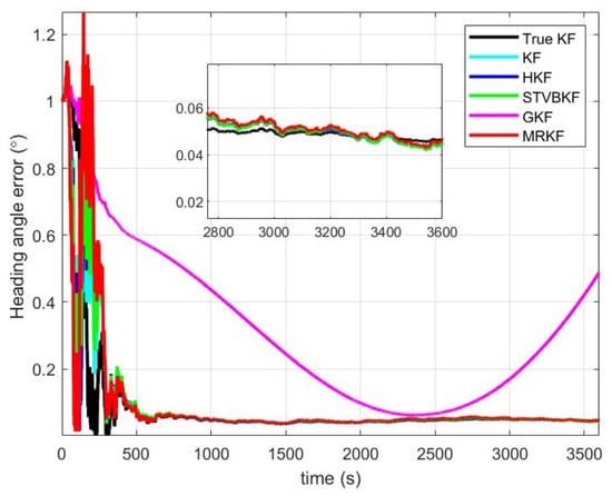
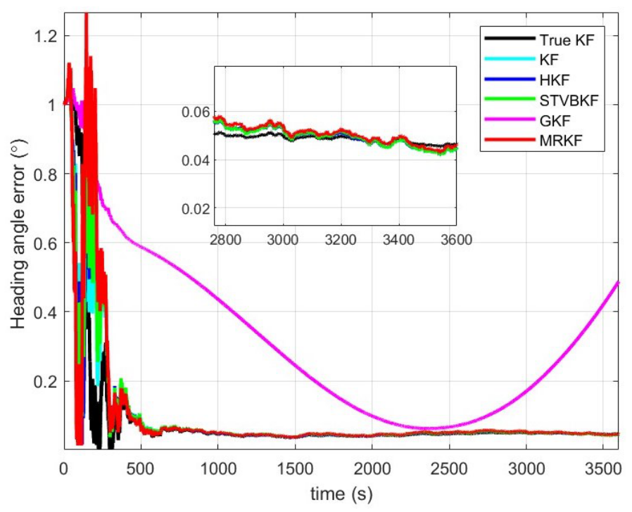
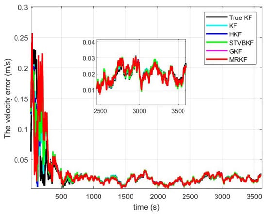
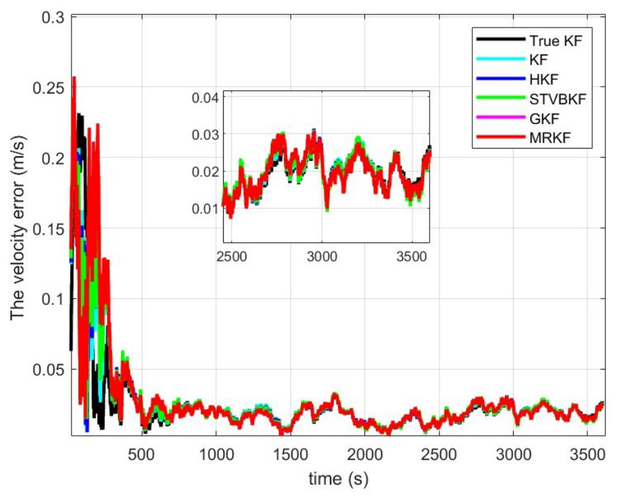
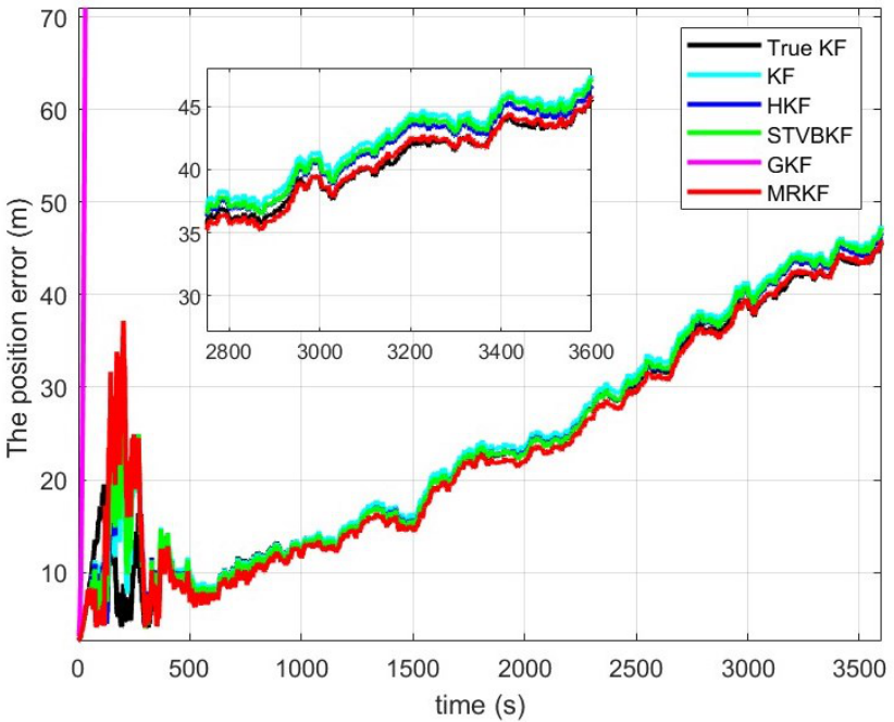
The first set of simulations is conducted under ideal conditions. In this case, the DVL operates normally and is not affected by abnormal interference. The initial parameters of the True KF is set as follows: the initial state is set as ${\mathbf{x}}_{\mathbf{0}}={\mathbf{0}}_{\mathbf{16}}$, and state noise and the covariance matrices of initial state error are set as ${\mathbf{Q}}_{\mathbf{0}}=\mathrm{diag}{\left([\mathbf{0}.{\mathbf{001}}^{\circ }/\sqrt{\mathrm{h}}{\mathbf{I}}_{\mathbf{3}\times \mathbf{1}};\mathbf{10}\mu \mathrm{g}/{\sqrt{\mathbf{Hz}}}_{\mathbf{3}\times \mathbf{1}}]\right)}^{\mathbf{2}}$ and ${\mathbf{P}}_{\mathbf{0}}=\mathrm{diag}{\left(\left[\mathbf{0}.{\mathbf{1}}^{\circ }{\mathbf{I}}_{\mathbf{3}\times \mathbf{1}};\mathbf{0}.\mathbf{1}\mathrm{m}/\mathrm{s}{\mathbf{I}}_{\mathbf{3}\times \mathbf{1}};\mathbf{2}\mathrm{m}{\mathbf{I}}_{\mathbf{3}\times \mathbf{1}};\mathbf{0}.{\mathbf{01}}^{\circ }/\mathrm{h}{\mathbf{I}}_{\mathbf{3}\times \mathbf{1}};\mathbf{100}/\mu \mathrm{g}{\mathbf{I}}_{\mathbf{3}\times \mathbf{1}};\mathbf{0}.\mathbf{001}\right]\right)}^{\mathbf{2}}$, respectively. The measurement noise covariance matrices is set as ${\mathbf{R}}_{\mathbf{0}}=\mathrm{diag}{\left([\mathbf{0}.\mathbf{1}\mathbf{m}/\mathbf{s}{\mathbf{I}}_{\mathbf{3}\times \mathbf{1}}]\right)}^{\mathbf{2}}$. Therefore, the True KF is used as an ideal reference benchmark because it adopts the true noise statistics in the simulation. In practical applications, however, the exact navigation-parameter errors and sensor-error statistics are usually unavailable. To simulate the parameter uncertainty in practical filtering, the covariance matrices used by KF, HKF, STVBKF, GKF, and MRKF are randomly inflated from the true covariance matrices by scale factors uniformly distributed in the interval [1, 10]. The same perturbed covariance settings are used for all practical filters in each simulation run to ensure a fair comparison. The simulation results are shown in Figure 1, Figure 2 and Figure 3.

Figure 1. Heading angle error results in the first simulation.

Figure 2. Velocity root mean square error results in the first simulation.

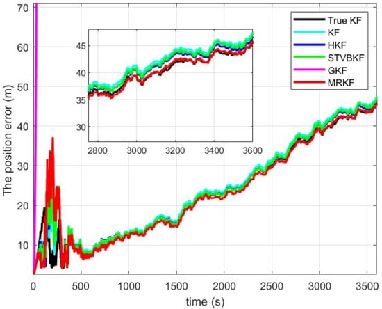
Figure 3. Position root mean square error results in the first simulation.

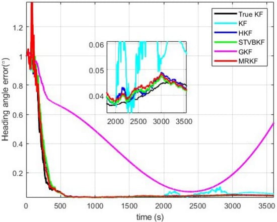
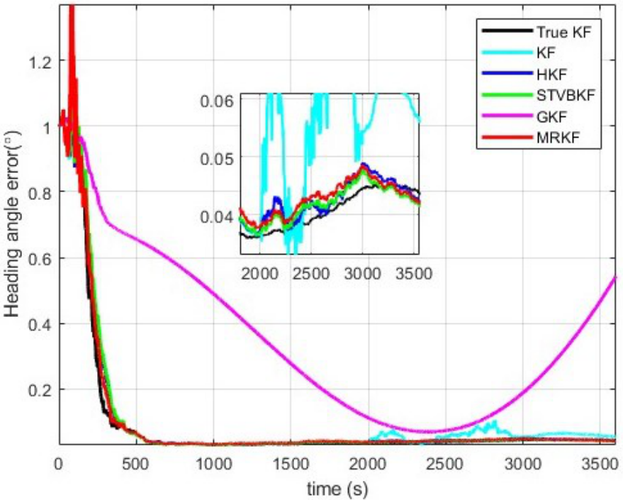
As can be seen from , the first 500 s mainly correspond to the initial convergence stage. After approximately 500 s, the filtering results become close to steady state, and the proposed method, KF, HKF, and STVBKF can all achieve satisfactory heading angle, velocity, and position estimation results. Since the DVL provides velocity rather than absolute position measurements, it can suppress the divergence of SINS velocity errors and partially constrain attitude errors, but it cannot directly correct the accumulated position error. Therefore, the position RMSE is not expected to converge to zero. In contrast, the GKF shows a larger estimation error even in the absence of injected DVL outliers. This is because the innovation during the initial convergence stage may be enlarged by dynamic transient errors and imperfect covariance settings. The hard innovation gate may therefore misclassify valid DVL measurements as outliers and reject them. Once the DVL updates are repeatedly rejected, the filter becomes close to a prediction-only inertial propagation mode, leading to increased navigation errors. Besides, according to the position error estimation results, the proposed method can obtain estimation results closest to those of KF and True KF under ideal conditions. It can achieve relatively high estimation accuracy under Gaussian-distributed noise conditions, thereby avoiding the degradation of state estimation accuracy caused by using the Student’s-t distribution model or robust filtering under Gaussian-distributed conditions.

(2)

The Second Simulation Test

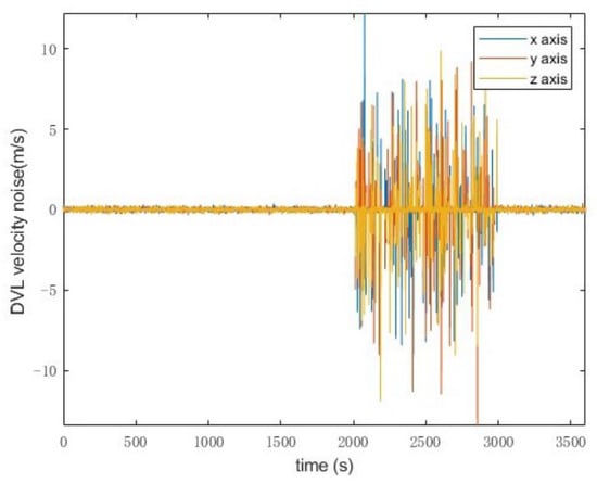
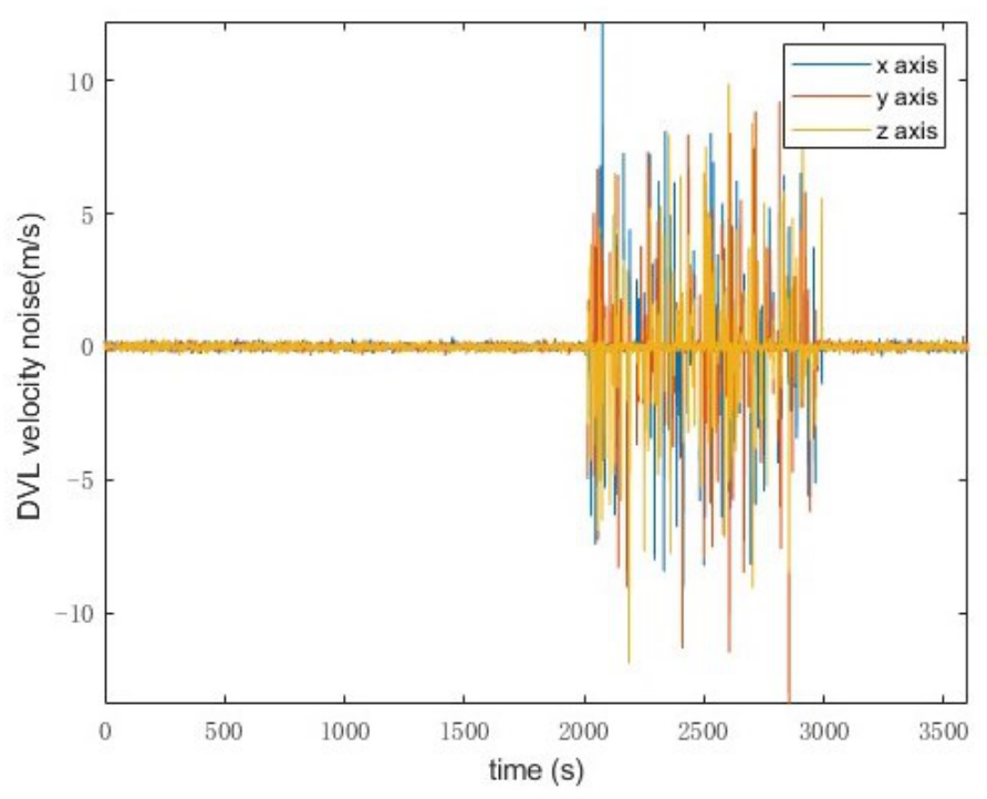
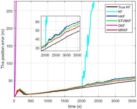
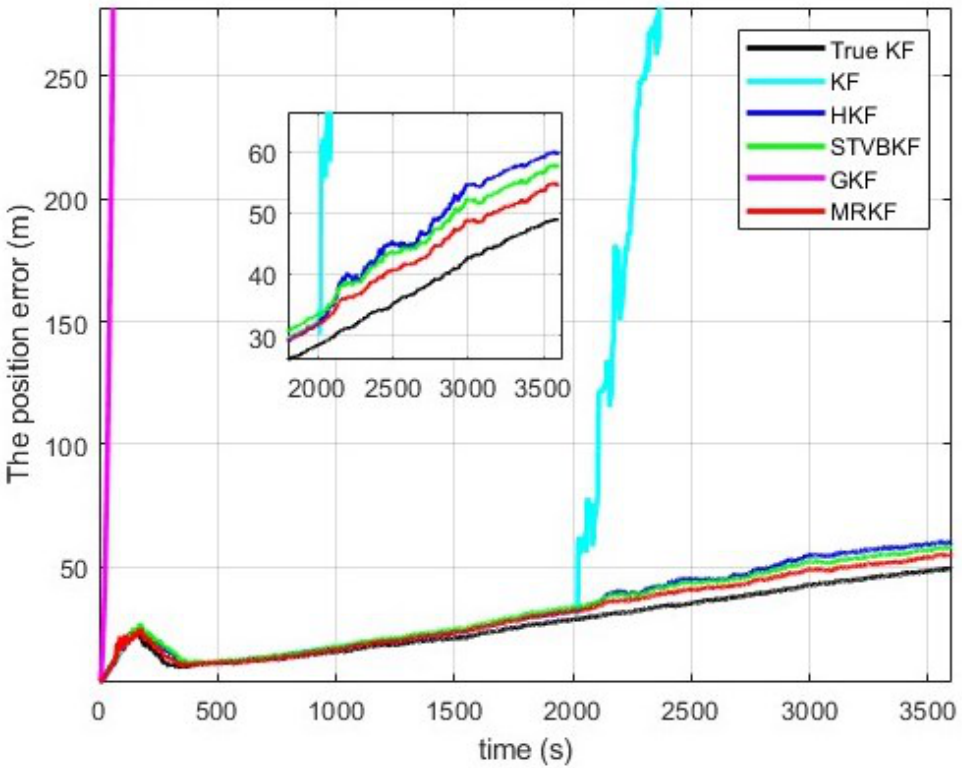
The second set of simulations is designed to simulate abnormal conditions occurring during part of the time period. The anomaly injection setting is shown in Figure 4. During the interval from $2000\mathrm{s}$ to $3000\mathrm{s}$, random DVL outliers are injected with an occurrence probability of 0.2. The outlier amplitude is uniformly distributed between 25 and 50 times the nominal DVL noise standard deviation, so that the injected anomalies represent gross DVL measurement disturbances rather than small Gaussian fluctuations. The lower bound is not set to zero because small deviations are already covered by the nominal Gaussian measurement-noise model. The initial filtering parameters in the second simulation are the same as those in the first simulation. For the True KF, however, the measurement noise covariance ${\mathbf{R}}_k$ is adjusted according to the actual abnormal DVL interference during the outlier-injection interval from 2000 s to 3000 s. This setting means that the True KF has prior knowledge of the true time-varying measurement-noise statistics and is therefore used only as an ideal reference benchmark. For KF, HKF, STVBKF, GKF, and the proposed MRKF, the true outlier information is assumed to be unknown, and the initial covariance matrices are set by the same random-inflation strategy used in the first simulation. Ten integrated navigation simulation tests are carried out in the second simulation. To ensure a fair and reproducible comparison, all random quantities were generated by a pseudorandom number generator. Different random noise sequences are generated for different repeated simulation runs, while the same sensor-noise sequence, covariance perturbation, and DVL outlier sequence are used by all compared algorithms within each single run. The statistical results of the root mean square errors (RMSE) of attitude, velocity, and position are shown in Table 2 and Figure 5, Figure 6 and Figure 7.

Figure 4. DVL output anomaly injection.

Table 2. RMSE statistics of navigation errors after 100 s in the second simulations.

Method	Heading Error ${(}^{\circ })$	Velocity Error $(\mathbf{m}/\mathbf{s})$	Position Error $\left(\mathbf{m}\right)$
True KF	0.042	0.023	47.99
KF	0.056	0.271	878.75
HKF	0.042	0.023	58.84
STVBKF	0.042	0.023	56.49
GKF	0.292	418.03	284,115.9
MRKF	0.042	0.023	53.39

Figure 5. The RMSE of heading angle results in the second simulation.

Figure 6. The RMSE of velocity results in the second simulation.

Figure 7. The RMSE of position results in the second simulation.

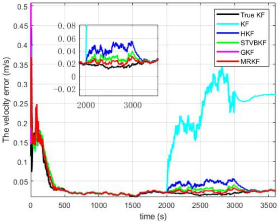
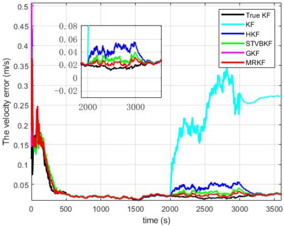
The first 500 s correspond to the normal initial convergence process, while the robustness comparison is mainly concerned with the DVL outlier-injection interval from 2000 s to 3000 s. As can be seen from Figure 5, Figure 6 and Figure 7and Table 2, during the time interval from $2000\mathrm{s}$ to $3000\mathrm{s}$, when abnormal interference occurs in the DVL output, the KF-based integrated navigation method lacks robustness and is most affected by the abnormal interference. Its heading error, velocity error, and position error all exhibit relatively large deviations. The GKF can reject part of the abnormal DVL measurements through hard innovation gating. However, its performance is sensitive to the selected chi-square threshold and the binary accept/reject decision. The integrated navigation methods based on HKF, STVBKF, and MRKF all exhibit a certain degree of robustness and can resist the influence caused by abnormal interference. Among them, STVBKF and MRKF can adaptively learn the measurement model, and therefore achieve better robustness and state estimation accuracy than HKF. In addition, MRKF takes into account both the high accuracy under Gaussian-distributed conditions and the robustness under abnormal interference conditions. It should be noted that the True KF is an ideal reference benchmark rather than a practical algorithm, since it uses prior knowledge of the true noise statistics. Therefore, the proposed MRKF is not expected to outperform the True KF. As shown in Table 2, the position RMSE of MRKF is $53.39\mathrm{m}$, which is close to that of the True KF, and is reduced by approximately $93.9\%$, $9.3\%$, and $5.5\%$ compared with KF, HKF, and STVBKF, respectively. Considering the total traveled distance of approximately $36\mathrm{km}$, this error corresponds to about $0.15\%$ of the trajectory length. Although MRKF requires additional computation because both the Gaussian branch and the Student’s-t branch are calculated before moment-matching fusion, the robust update is performed only at the DVL sampling rate of $1\mathrm{Hz}$. Therefore, the additional computational cost is acceptable for the considered SINS/DVL integrated navigation system.

In summary, the proposed method achieves a favorable trade-off between estimation accuracy under nominal Gaussian noise and robustness against abnormal DVL outliers, making it more suitable for SINS/DVL integrated navigation.

5. Conclusions

Aiming at the problem of DVL outlier interference in SINS/DVL integrated navigation, this paper proposes a MRKF based on Gaussian–Student’s-t mixed noise modeling and soft-gating dual-branch fusion. The proposed MRKF combines the high estimation accuracy of the standard KF under nominal Gaussian noise with the robustness of the Student’s-t filter under abnormal interference. An innovation-driven logistic soft-gating mechanism is designed to adaptively fuse the two posterior distributions through moment matching, thereby avoiding the discontinuity caused by hard-threshold switching. The simulation results show that, under the considered one-hour SINS/DVL integrated navigation simulation, the proposed MRKF maintains high estimation accuracy under nominal Gaussian noise and effectively suppresses the influence of injected DVL outliers. Compared with KF, HKF, and STVBKF, the proposed MRKF achieves better overall navigation performance in the designed outlier-interference scenario. These results indicate that the proposed MRKF provides a promising trade-off between nominal estimation accuracy and robustness against DVL outliers. Future work will focus on lake or sea-trial validation, adaptive parameter optimization, and extension to nonlinear and time-varying noise scenarios.

References

- Luo, L.; Huang, Y.; Chang, L.; Zhang, Y. Development and prospects of initial alignment method for strap-down inertial navigation system. Chin. J. Ship Res. 2022, 17, 301–313. [Google Scholar]
- Xu, G.; Huang, Y.; He, Y.; Luo, L.; Zhang, Y. Transfer Alignment for Inertial Navigation System: A Review and Future Direction. Unmanned Syst. Technol. 2022, 3, 64–78. [Google Scholar]
- Chang, L.; Bian, Q.; Zuo, Y.; Zhou, Q. SINS/GNSS-integrated navigation based on group affine SINS mechanization in local-level frame. IEEE/ASME Trans. Mechatron. 2023, 28, 2471–2482. [Google Scholar]
- Tal, A.; Klein, I.; Katz, R. Inertial navigation system/Doppler velocity log (INS/DVL) fusion with partial DVL measurements. Sensors 2017, 17, 415. [Google Scholar] [PubMed]
- Yao, Y.; Xu, X.; Hou, L.; Deng, K.; Xu, X. A simple and precise correction method for DVL measurements under the dynamic environment. IEEE Trans. Veh. Technol. 2020, 69, 10750–10758. [Google Scholar] [CrossRef] [Scilit]
- Zhu, T.; Li, A.; Chang, L.; Li, K. Two-frame group error model for SINS/DVL integration: Analysis and comparison. IEEE Trans. Instrum. Meas. 2025, 74, 8501515. [Google Scholar]
- Luo, L.; Huang, Y.; Wang, G.; Zhang, Y.; Tang, L. An on-line full-parameters calibration method for SINS/DVL integrated navigation system. IEEE Sens. J. 2023, 23, 30927–30939. [Google Scholar]
- Xu, X.; Gui, J.; Sun, Y.; Yao, Y.; Zhang, T. A robust in-motion alignment method with inertial sensors and Doppler velocity log. IEEE Trans. Instrum. Meas. 2020, 70, 8500413. [Google Scholar] [CrossRef] [Scilit]
- Wang, D.; Wang, B.; Huang, H.; Yao, Y. An improved robust filter method for SINS/DVL system with Earth frame error model. IEEE Trans. Veh. Technol. 2024, 73, 12760–12772. [Google Scholar] [CrossRef] [Scilit]
- Karlgaard, C.D.; Schaub, H. Huber-based divided difference filtering. J. Guid. Control. Dyn. 2007, 30, 885–891. [Google Scholar] [CrossRef] [Scilit]
- Gandhi, M.A.; Mili, L. Robust Kalman filter based on a generalized maximum-likelihood-type estimator. IEEE Trans. Signal Process. 2009, 58, 2509–2520. [Google Scholar]
- Wang, Y.; Zheng, W.; Sun, S.; Li, L. Robust information filter based on maximum correntropy criterion. J. Guid. Control. Dyn. 2016, 39, 1126–1131. [Google Scholar] [CrossRef] [Scilit]
- Izanloo, R.; Fakoorian, S.A.; Yazdi, H.S.; Simon, D. Kalman filtering based on the maximum correntropy criterion in the presence of non-Gaussian noise. In Proceedings of the 2016 Annual Conference on Information Science and Systems (CISS); IEEE: Piscataway, NJ, USA, 2016; pp. 500–505. [Google Scholar]
- Graham, M.C.; How, J.P.; Gustafson, D.E. Robust state estimation with sparse outliers. J. Guid. Control. Dyn. 2015, 38, 1229–1240. [Google Scholar] [CrossRef] [Scilit]
- Nakajima, J.; Omori, Y. Stochastic volatility model with leverage and asymmetrically heavy-tailed error using GH skew Student’s t-distribution. Comput. Stat. Data Anal. 2012, 56, 3690–3704. [Google Scholar]
- Gustafsson, F.; Gunnarsson, F. Mobile positioning using wireless networks: Possibilities and fundamental limitations based on available wireless network measurements. IEEE Signal Process. Mag. 2005, 22, 41–53. [Google Scholar] [CrossRef] [Scilit]
- Arulampalam, M.S.; Maskell, S.; Gordon, N.; Clapp, T. A tutorial on particle filters for online nonlinear/non-Gaussian Bayesian tracking. IEEE Trans. Signal Process. 2002, 50, 174–188. [Google Scholar] [CrossRef] [Scilit]
- Huang, Y.; Zhang, Y.; Zhao, Y.; Chambers, J.A. A novel robust Gaussian–Student’s t mixture distribution based Kalman filter. IEEE Trans. Signal Process. 2019, 67, 3606–3620. [Google Scholar] [CrossRef] [Scilit]
- Jia, G.; Zhang, Y.; Huang, Y.; Bai, M.; Wang, G. A New Robust Student’s t Based SINS/GPS Integrated Navigation Method. In Proceedings of the 2018 International Conference on Control, Automation and Information Sciences (ICCAIS); IEEE: Piscataway, NJ, USA, 2018; pp. 285–290. [Google Scholar]
- Qian, M.; Chen, W.; Sun, R. A Student’s T Distribution-Based Filter Design for SINS/GNSS With Heavy-Tailed Noise. IET Electr. Power Appl. 2025, 19, e70076. [Google Scholar]
Disclaimer/Publisher’s Note: The statements, opinions and data contained in all publications are solely those of the individual author(s) and contributor(s) and not of MDPI and/or the editor(s). MDPI and/or the editor(s) disclaim responsibility for any injury to people or property resulting from any ideas, methods, instructions or products referred to in the content. |
© 2026 by the authors. Licensee MDPI, Basel, Switzerland. This article is an open access article distributed under the terms and conditions of the Creative Commons Attribution (CC BY) license.